Wave Optics Effects from Gravitational Wave Propagation Through Dark Matter Halos
June 29, 2026
Abstract
Gravitational wave (GW) propagation is usually studied under the geometric optics approximation. But when GWs propagate through structures of sizes similar to their wavelength, this approximation breaks down. Going beyond the geometric optics
approximation allows us to explore the wave optics effects in curved background that appear in such cases. In this work, we present a scheme for numerically evolving linearised plane GWs through stationary, spherical astrophysical structures in both weak
and strong gravity regimes. Our simulations evolve the full Einstein equations (with all 10 components) for Gaussian, NFW and Burkert potentials, although in simplified form for the two latter. Our simulations show that the scattering of the GWs depends
not only on the mass of the lens but also strongly on the gravitational potential distribution of the lens. We isolate the effects of diffraction by setting the wavelength of GW to be less than the Schwarzschild radius of the structure. Among our most
important results, we find that the GWs do not propagate along null geodesics when propagating through the Gaussian density, neither in the strong nor weak gravity setting. We also find that for the Burkert potential, the convexity of the plane wave is
flipped when leaving the structure, in the strong gravity case.
We compare our results with the linearized scalar wave predictions and find that the difference between these and the exact GW modes are of order one when the wave is inside the central potential. However, the difference reduces to only a few percent when
the wave has passed through the structure. Although these effects are small, future GW detectors and Pulsar Timing Arrays (PTAs) could be sensitive to these signals which could thus potentially help in constraining the structure of dark matter spikes or
halos.
Keywords: gravitational waves, dark matter, wave optics, numerical simulations
1 Introduction↩︎
The direct detection of gravitational waves (GWs) by the LIGO–Virgo–KAGRA collaboration [1]–[8] has opened a new observational window on the Universe, enabling the exploration of strong field predictions of general relativity and a large array of other endeavours within fundamental physics such as constraining the
graviton mass, detecting possible large extra dimensions, exploring dark matter properties and providing new insights to the Hubble tension (see e.g. [9],
[10] for reviews). In most observational and theoretical analyses, GW propagation is treated within the framework of geometric optics where it is assumed that the wavelength of the GW is much smaller
than the characteristic scale of any gravitational lens it encounters. Under this approximation, the effect of lensing reduces to a frequency-independent magnification and a time delay. However, in situations where the Schwarzschild radius of the lens is
comparable to or smaller than the wave length of the GW, wave optics becomes important and the geometric optics approximation breaks down [11]–[14]. In the wave optics regime, diffraction and interference modify the GW signal in a frequency-dependent manner, producing amplitude
modulations and phase shifts.
Theoretical work on wave optics for GWs has primarily relied on analytic approximations such as employing series expansions/perturbative methods [15]–[21], using simple lens models such as point lenses [16], [22], [23], and by evaluating diffraction integrals ([14], [18], [19], [24]) for scalar GWs and thin lenses, traditionally restricting to the small-angle regime (see e.g. the introduction of [25] for a review on shortcomings of analytical approaches in the literature). Such studies demonstrate that
wave optics signatures carry information about the mass, structure, and spatial distribution of the lensing object ([11], [19], [26], [27]), and can be utilized to probe dark matter and small-scale structures in the Universe ([28]–[34]). Although analytical methods offer valuable insights, they are thus often restricted to idealized geometries and cannot easily accommodate complex or time-dependent lens configurations. But realistic astrophysical
environments are characterized by complex, inhomogeneous matter distributions that cannot readily be captured by the idealized lens models usually considered in analytical studies. The general shapes, substructures, and clustering of matter can lead to
rich and distinctive wave-optics effects such as diffraction, interference, and mode conversion, that are too complicated to study analytically. Numerical approaches are essential for accurately modelling these effects when considering gravitational wave
propagation in realistic cosmological settings and thus for interpreting future observations. Thus, to fully understand to what extent wave optics affects our interpretation of GW signals in terms of e.g. inferring lens properties or cosmological
parameters [35], [36], we should ideally move beyond
the simplified analytical treatments, and study more complex systems with numerical relativity. However, simulations face significant challenges of their own: The need to resolve both the wavelength of the GW and the macroscopic scales of the lens, the
computational cost of high-resolution wave propagation, and the difficulties of handling arbitrary lens geometries. Significant progress has been made on the numerical front for standard astrophysical configurations. For instance, [37] performed numerical propagation of GWs through a potential well, although without considering curvature corrections. Another notable work in this regard is [38], where the authors developed a Python package that offers solutions for GW lensing
computations within the full wave-optics regime. But this work uses 2 dimensional diffraction integrals with small angle approximation and hence does not capture effects such as polarization mixing, mode coupling due to curvature terms, wave scattering due
to curvature, tail formation and Lorenz gauge preservation.
As gravitational wave detectors continue to improve in sensitivity, the lensing of gravitational waves by intervening matter is expected to become increasingly relevant ([39]–[49]. The current ground based observatories LIGO, Virgo and Kagra are sensitive to the frequency range \(10\)Hz - \(10\)kHz. For these wave lengths, wave optics effects occur when the waves propagate through structures with mass around or below \(10^4\;M_\odot\).
Astrophysical objects with mass in this range include stars and low mass compact object remnants like white dwarfs, neutron stars, black holes and primordial black holes. Future space based GW detectors like LISA [50] and DECIGO [51] are sensitive to
frequencies \(0.1\)mHz - \(100\)mHz and \(1\)mHz - \(100\)Hz, respectively. Here, the lens masses that are relevant for wave
optics effects go up to \(10^9 M_\odot\). Objects in this mass range include dark matter subhalos and larger compact structures [52]. Pulsar Timing Arrays (PTA) are sensitive to ultra low frequency GWs of nano-Hz or micro-Hz which have very high wavelength that are affected by wave optics due to cosmological structures and dark matter halos.
In this work, we present a numerical framework for studying GW propagation in the wave optics regime. Our approach solves the full Einstein equation for the linearized tensor perturbations corresponding to the GW. In contrast to the previous works like
[53], where the authors propagate GWs through a black hole, we propagate GWs through a Gaussian density distribution to mimic propagation through a dark
matter halo structure.Additionally, we consider the importance of the halo shape by comparing results obtained by considering GW propagation through Gaussian, Navarro–Frenk–White (NFW) [54] and Burkert [55] gravitational potential distributions. We use the
CarpetX framework of the Einstein Toolkit[56], [57] for the evolution with Adaptive Mesh Refinement (AMR) capabilities. This enables our simulations to accurately model interference and lensing effects for a wide range of astrophysical scenarios. Our simulations can be
used to make realistic models of GW propagation and hence e.g. more realistic training data for Machine Learning efforts. The results from these simulations can also be used for consistency checks of simplified analytical methods so that these can be
tested in more complex situations than what is usually done, where comparison is made with e.g. point lenses.
The paper is organized as follows: In section 2 we review Einstein’s equation for linearized GWs in a curved background spacetime. We then consider a background spacetime with metric perturbations and derive
the evolution equation for GWs propagating on this “background”. In section 3 we describe our numerical setup and numerical methods involved in solving this set of equations including setting up initial
conditions. In section 4 we report our findings for GW propagation through a Gaussian density distribution in both the weak and strong gravity setting, while section 5 reports the findings for solution to the propagation equations for a GW propagating through a scalar potential corresponding to a NFW and Burkert density profile, but where the density itself is ignored as
detailed in the section. Sec. 6 is dedicated to conclusions, including a discussion of possible future extensions.
Throughout this paper, we adopt geometrized units with \(G=1=c\), where space and time have the same units which we here adopt to be mass \(M\).
2 Theoretical setup↩︎
Similar to light propagation studies, most gravitational lensing studies apply the geometric optics approximation. In this approximation, one assumes that the light/GW wavelength is much smaller than the length scale over which the amplitude,
polarization and radius of curvature change [58]. However, when the wavelength is comparable to the radius of curvature of the
background, wave optics effects become prominent and the geometric optics approximation fails. We here study the appearance of such wave-optics phenomena by numerically propagating gravitational waves through steep curvature gradients. For describing the
spacetime around an astrophysical structure such as a dark matter halo, we assume that the background metric upon which the GW propagates takes the form \[g^B_{\mu \nu} = \text{diag}[
\;-\exp(2\phi)dt^2 + \exp(-2\phi) (dx^2 +dy^2 +dz^2) \;], \label{metric95exp}\tag{1}\] where \(\phi\) is a gravitational potential obtained by solving the Poisson equation sourced by the central density of the
halo. The metric of this form is more appropriate for capturing non-linear curvature terms compared to the usual linearly perturbed perturbed metric of the form (considering only scalar perturbations for now) \[g_{\mu \nu} = \text{diag}[ \;-(1 + 2\phi)dt^2 + (1 - 2\phi) (dx^2 +dy^2 +dz^2) \;]
\label{metric}\tag{2}\] and is e.g. used in the weak-field approximation of the relativistic N-body simulation gevolution [59]. Assuming the line element of equation 1 , Einstein’s equation for the linearized trace-reversed metric perturbation satisfying the Lorentz gauge condition \(\nabla_{\mu} \bar h^{\mu \nu} = 0\) is [60] \[\begin{align} \nabla^{\alpha} \nabla_{\alpha} \bar h_{\mu \nu} + 2 R^B_{\alpha \mu \beta \nu} \bar h^{\alpha \beta} = - 16 \pi \;\bigg( \mathcal{T}_{\mu \nu} - \frac{1}{2} \bar{h}_{\alpha \beta} T_B^{\alpha \beta} g^B_{\mu \nu} \\
-\frac{1}{2} \bar{h} T^B_{\mu \nu} + \frac{1}{4} \bar{h} \;T_B \;g^B_{\mu \nu} \bigg) \label{gweqn}
\end{align}\tag{3}\] where \(\bar h_{\mu \nu} = h_{\mu \nu} - \frac{1}{2} h g^B_{\mu \nu}\) is the trace-reversed metric perturbation, \(\mathcal{T}_{\mu \nu}\) is the
stress-energy-momentum tensor, \(\bar h \equiv \bar{h}_{\alpha \beta} g_B^{\alpha \beta}\) and \(T_B = T_B^{\alpha \beta} g^{B}_{\alpha \beta}\).
Expanding the first term in the Left-hand-side of equation 3 yields \[\begin{align} \bar{h}_{\mu \nu ; \alpha}^{\;; \alpha} =\; & g_B^{\alpha \beta} \bigg[
\partial_\beta \partial_\alpha \bar{h}_{\mu \nu}
- \partial_\beta \left( \Gamma^\lambda_{\alpha \mu} \bar{h}_{\lambda \nu} \right)
- \partial_\beta \left( \Gamma^\lambda_{\alpha \nu} \bar{h}_{\mu \lambda} \right) \\
& - \Gamma^\lambda_{\beta \alpha} \partial_\lambda \bar{h}_{\mu \nu}
+ \Gamma^\lambda_{\beta \alpha} \Gamma^\sigma_{\lambda \mu} \bar{h}_{\sigma \nu}
+ \Gamma^\lambda_{\beta \alpha} \Gamma^\sigma_{\lambda \nu} \bar{h}_{\mu \sigma} \\
& - \Gamma^\lambda_{\beta \mu} \partial_\alpha \bar{h}_{\lambda \nu}
+ \Gamma^\lambda_{\beta \mu} \Gamma^\sigma_{\alpha \lambda} \bar{h}_{\sigma \nu}
+ \Gamma^\lambda_{\beta \mu} \Gamma^\sigma_{\alpha \nu} \bar{h}_{\lambda \sigma} \\
& - \Gamma^\lambda_{\beta \nu} \partial_\alpha \bar{h}_{\mu \lambda}
+ \Gamma^\lambda_{\beta \nu} \Gamma^\sigma_{\alpha \mu} \bar{h}_{\sigma \lambda}
+ \Gamma^\lambda_{\beta \nu} \Gamma^\sigma_{\alpha \lambda} \bar{h}_{\mu \sigma}
\bigg],
\end{align}\] where the Christoffel symbols are computed with respect to the background metric \(g^B_{\mu \nu}\).
Similarly, the second term of equation 3 can be expanded to (ignoring the overall factor of 2) \[\begin{align}
R^B_{\alpha\mu\beta\nu} \bar h^{\alpha\beta} &= g^B_{\alpha \delta} \;(
\partial_{\beta}\Gamma^{\delta}{}_{\nu\mu}
- \partial_{\nu}\Gamma^{\delta}{}_{\beta\mu}
\\
&+ \Gamma^{\delta}{}_{\beta\lambda}\Gamma^{\lambda}{}_{\nu\mu}
- \Gamma^{\delta}{}_{\nu\lambda}\Gamma^{\lambda}{}_{\beta\mu} \;) \;g_B^{\rho\alpha} \;g_B^{\sigma\beta} \;\bar h_{\rho\sigma}
\end{align}\] In addition, in equation 3 we assume that the stress-energy-momentum tensor contribution from GWs are significantly smaller than the background contributions so that we may ignore this contribution. The
evolution equations in terms of the trace-reversed metric perturbation are thus: \[\begin{align}
g_B^{\alpha \beta} \bigg[
\partial_\beta \partial_\alpha \bar{h}_{\mu \nu}
- \partial_\beta \left( \Gamma^\lambda_{\alpha \mu} \bar{h}_{\lambda \nu} \right)
- \partial_\beta \left( \Gamma^\lambda_{\alpha \nu} \bar{h}_{\mu \lambda} \right) \\
- \Gamma^\lambda_{\beta \alpha} \partial_\lambda \bar{h}_{\mu \nu}
+ \Gamma^\lambda_{\beta \alpha} \Gamma^\sigma_{\lambda \mu} \bar{h}_{\sigma \nu}
+ \Gamma^\lambda_{\beta \alpha} \Gamma^\sigma_{\lambda \nu} \bar{h}_{\mu \sigma} \\
- \Gamma^\lambda_{\beta \mu} \partial_\alpha \bar{h}_{\lambda \nu}
+ \Gamma^\lambda_{\beta \mu} \Gamma^\sigma_{\alpha \lambda} \bar{h}_{\sigma \nu}
+ \Gamma^\lambda_{\beta \mu} \Gamma^\sigma_{\alpha \nu} \bar{h}_{\lambda \sigma} \\
- \Gamma^\lambda_{\beta \nu} \partial_\alpha \bar{h}_{\mu \lambda}
+ \Gamma^\lambda_{\beta \nu} \Gamma^\sigma_{\alpha \mu} \bar{h}_{\sigma \lambda}
+ \Gamma^\lambda_{\beta \nu} \Gamma^\sigma_{\alpha \lambda} \bar{h}_{\mu \sigma}
\bigg] \\
+ \; 2 \;g^B_{\alpha \delta} \;(
\partial_{\beta}\Gamma^{\delta}{}_{\nu\mu}
- \partial_{\nu}\Gamma^{\delta}{}_{\beta\mu}
+ \Gamma^{\delta}{}_{\beta\lambda}\Gamma^{\lambda}{}_{\nu\mu} \\
- \Gamma^{\delta}{}_{\nu\lambda}\Gamma^{\lambda}{}_{\beta\mu} \;) \;g_B^{\rho\alpha} \;g_B^{\sigma\beta} \;\bar h_{\rho\sigma} = 8 \pi \;\bigg( \bar{h}_{\alpha \beta} T_B^{\alpha \beta} g^B_{\mu \nu} \\ + \;\bar{h} T^B_{\mu \nu} - \frac{1}{2} \bar{h} \;T_B
\;g^B_{\mu \nu} \bigg) .
\end{align}
\label{evol}\tag{4}\] The constraint violation (the Lorenz gauge condition) reads \[\mathcal{C}_{\nu} =\nabla^{\mu} \bar h_{\mu \nu} = g_B^{\nu \rho} ( \;\partial_{\rho}{ \bar h_{\mu
\nu} } - \Gamma^{\lambda}_{\mu \rho} \bar h_{\lambda \nu} - \Gamma^{\lambda}_{\nu \rho} \bar h_{\mu \lambda} \;).
\label{cv}\tag{5}\] In addition to the evolution equations 4 , we also evolve the linearly approximated scalar wave equation defined by \(g_
B^{\alpha \beta}
\partial_\beta \partial_\alpha h_{\mu \nu}\) which does not include curvature terms (Christoffel symbols and its derivatives ), i.e., \[\left[ \exp(2 \phi)^{-1}\partial_{tt} -
\exp(- 2 \phi)^{-1}( \partial_{xx} + \partial_{yy} + \partial_{zz}) \right] h = 0. \label{simplified95evol}\tag{6}\] Evolving 6 and comparing the results with 4 will allow us to
distinguish the contributions from the curvature terms.
In the next section we will describe our numerical setup used to evolve equations presented above.
3 Numerical setup↩︎
In this section, we describe our numerical setup used to evolve the evolution equations derived in the previous section. We will run six simulations that propagate initially plane-parallel and spherical gravitational waves through three different spherical potential fields motivated by models of dark matter halos.
In subsection 3.1 we describe our code architecture and numerical methods, in subsection 3.2 we discuss the three density profiles we consider, and in subsection 3.3 we describe our initial conditions. In subsections 3.5 and 3.4 we present the numerical schemes adopted for constraint damping and Adaptive Mesh Refinement(AMR).
3.1 Numerical evolution in 3+1D↩︎
The linear GWs equation in curved spacetime are a set of two independent coupled second order linear hyperbolic partial differential equations (PDEs). By substitution, we convert the second order time derivatives into first order derivatives, yielding
two coupled first order PDEs. Thus, in total we evolve 10 components of the metric perturbation \(\bar h_{\mu \nu}\) and another 10 components of \(d_t \bar h_{\mu \nu}\). We use
Cadabra [61]–[63], an open-source computer algebra software package to expand the tensor equations 4 . We then use Sympy-bridge in Cadabra to convert the equations into expressions
compatible with C++. The equations are then evolved in time using a fourth order Runge Kutta time integrator. To compute the gradients and divergences appearing in the ten PDEs, we use the Method of Lines [64] to discretize in all but one dimension. This leads to a system of ordinary differential equations (ODEs) where we can use a fourth order central
finite difference stencil to compute the derivatives. We use Einstein Toolkit’s CarpetX framework to evolve this set of four coupled space and time-discretized ODEs. We make use of Adapative-Mesh-Refinement (AMR) capabilities of
CarpetX to resolve the regions that have steep curvature gradients.
As we are only interested in the simulation domain’s interior, we use symmetric, reflecting boundary conditions in all directions. We stop the simulation when the wave reaches close to the end of the simulation box to prevent reflected waves from affecting
our results. To be conservative of our computational resources, we propagate plane wave that are constant in \(x-y\) axis in a rectangular simulation domain.
3.2 Considered densities and corresponding potentials↩︎
We consider three different spherical mass density profiles for our simulations, namely a Gaussian profile, the Navarro–Frenk–White (NFW) profile [54] and Burkert density profile [55]. The Gaussian profile mimics the usual spherical mass distribution whereas
the NFW and Burkert profiles are common models of the shape of cold dark matter haloes and dwarf galaxies, respectively. Specifically, we consider the profiles defined as
\[\rho(r)= \begin{cases} \frac{M}{ \lambda^3 (2\pi)^{3/2} } \cdot \exp( -\frac{r^2}{2 \lambda^2}), & \text{Gaussian} \\[1em] \frac{\rho_{0}}{\frac{r}{R_s}\left( 1 + \frac{r}{R_s} \right)^2}, & \text{NFW profile } \\[1em]
\frac{\rho_{0} R_s^3}{(r + R_s)\left( r^2 + R_s^2 \right)}, & \text{Burkert profile}, \end{cases}\]
where \(\lambda\) determines the spread of the Gaussian density, \(\rho_0 \equiv M/4 \pi R_s^3\), and \(R_s\) is the scale radius that sets the size of halo
structure.
The expressions for \(\rho(r)\) for the NFW and Burkert profiles diverge for \(r \rightarrow0\). For these two profiles, we therefore solve the simplified system of Einstein’s equation 4 with the right hand side set to zero i.e with \(T^B_{\mu \nu} = 0\). We will refer to the resulting equations as the density-free equations. These still capture the effects of curvature that results in
mode mixing and curvature scattering. Furthermore, for the Gaussian profile, we will solve both the equations with the correct density in the right hand side as well as the density-free equations, to quantify how big an effect setting \(T_{\mu\nu} = 0\) has on our results.
We obtain the gravitational potential by solving the Poisson equation \(\nabla^2 \phi(r) = 4\pi \rho(r)\). For the NFW and Burkert profile, although the densities diverge as \(r
\rightarrow0\), the potential \(\phi\) converges as \(r \rightarrow0\). Specifically, the corresponding expressions for \(\phi\) are
\[\phi(r) = \begin{cases} -\dfrac{M_{\text{gauss}}}{r} \cdot \operatorname{erf}\!\left(\dfrac{r}{\sqrt{2}\,\lambda}\right), & \text{Gaussian} \\[1em] -\dfrac{M_{\text{NFW}}}{r} \ln\!\left(1 + \dfrac{r}{R_s}\right), & \text{NFW profile \cite{GalRotpy}} \\[1em] \dfrac{M_{\text{bk}}}{4 R_s} \Bigg\{ \Big(1 - \dfrac{R_s}{r}\Big) \ln\!\Big(1 + \Big(\dfrac{r}{R_s}\Big)^2\Big) + 2\Big(1 + \dfrac{R_s}{r}\Big)\Big[\tan^{-1}\!\Big(\dfrac{r}{R_s}\Big) - \ln\!\Big(1 + \dfrac{r}{R_s}\Big)\Big] - \pi \Bigg\}, & \text{Burkert profile\cite{GalRotpy}} \end{cases}\]
where we defined \(M_{\text{gauss}} := \phi_{\text{max}}\lambda \sqrt\frac{\pi}{2}\), \(M_{\text{NFW}} := R_s \phi_{\text{max}}\) and \(M_{\text{bk}} := \dfrac{4
R_s}{\pi} \phi_{\text{max}}\). Here, \(\phi_{\text{max}}\) is the maximum value \(\phi\) takes, and setting it to a specific value allows us to compare simulations among these
different profiles. In equation 2 , setting \(\phi=0\), corresponds to flat spacetime and \(|\phi| = -1/2\) results in formation of a horizon-like surface similar to
a black hole. Thus, a weak gravity regime is obtained by setting \(|\phi|\) slightly above zero while the strong gravity regime is probed with \(|\phi|\) close to 1/2. For our simulations,
we consider simulations, we probe both situations by considering first \(\phi_{\text{max}} = -0.1\) and then \(\phi_{\text{max}} = -0.49\), respectively.
Figures 1 show derivatives of \(\phi(r)\) along the z-axis in the simulation grid box.
For the simulations with the Gaussian density distribution, we assume the matter to be pressure-less (mimicking cold dark matter) and hence \(T_{\mu \nu}^B = \text{diag}[\rho_{\text{gauss}} \exp(2 \phi),0,0,0]\).
3.3 Initial conditions for the wave↩︎
We consider circularly polarized monochromatic waves propagating along the z-axis as our initial condition. These waves can e.g. represent GWs originating from binary compact object coalescence or stochastic GWs permeating through space. We initialize
them at a specific distance from the central density and let them propagate through the curved spacetime near the centre of our simulation box. The initial strain of \(h_+ = h_{xx} = -h_{yy}\) and \(h_\times = h_{xy} = h_{yx}\) are set as \[\label{ic95planewave} \begin{align} h_+ & = \mathcal{A} \cos[ 2 \pi (k_zz-\omega t)] \\ h_\times & =
\mathcal{A} \sin[ 2 \pi (k_zz-\omega t)]. \\ \end{align}\tag{7}\] Here, \(\mathcal{A}\) is the amplitude of the wave and \(\omega = \sqrt{k_x^2+k_y^2+k_z^2} = |k_z|\).
For a full evolution of Einstein’s equation 3 in curved spacetime, we need initial conditions for all the ten components of \(\bar h_{\mu \nu}\) and another ten initial conditions for its time
derivatives satisfying the constraints in equation 5 . Specifying only the above plane wave initial condition in equation 7 along with its derivatives results in under-determined initial conditions.
Although we could use equation 5 to determine the other components, this is non-trivial since it requires careful consideration not to introduce spurious gauge modes. To avoid this, we initialize the wave in a confined region in flat
Minkowski background similar to the approach in [65]. Specifically, we introduce a quintic spline at a finite distance from the central
density and use it to smoothly force the gravitational potential \(\phi\) and its derivatives \(\phi'\) and \(\phi''\) to zero. Our potential is
thus given by \[\phi(r)= \begin{cases} \phi(r), & \text{if } r\leq r_1\\ \text{Spline approximation}, & \text{if } r_1 \leq r \leq r_2 \\ 0, & \text{if } r \geq r_2,
\end{cases}\] where \(r = \sqrt{x^2 + y^2 +z^2}\) and \(r_1\), \(r_2\) are set by hand. In table 2 we list the values of
\(r_1\) and \(r_2\) used in our simulations. In figure 1 we present the derivatives of \(\phi\) for each potential
configuration for the case of strong gravity and we note that the behaviour of the derivatives remains similar for the weak gravity case.
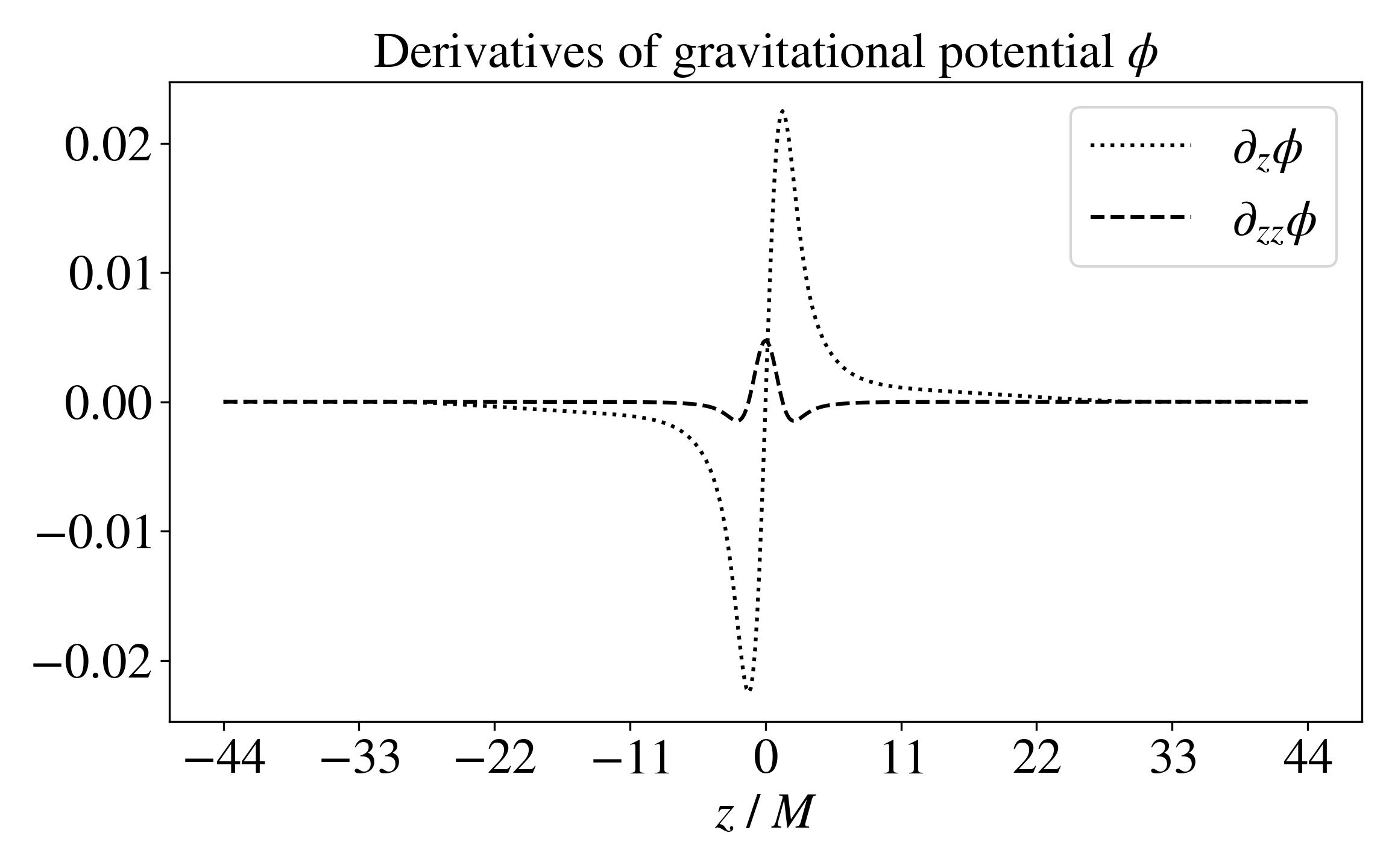
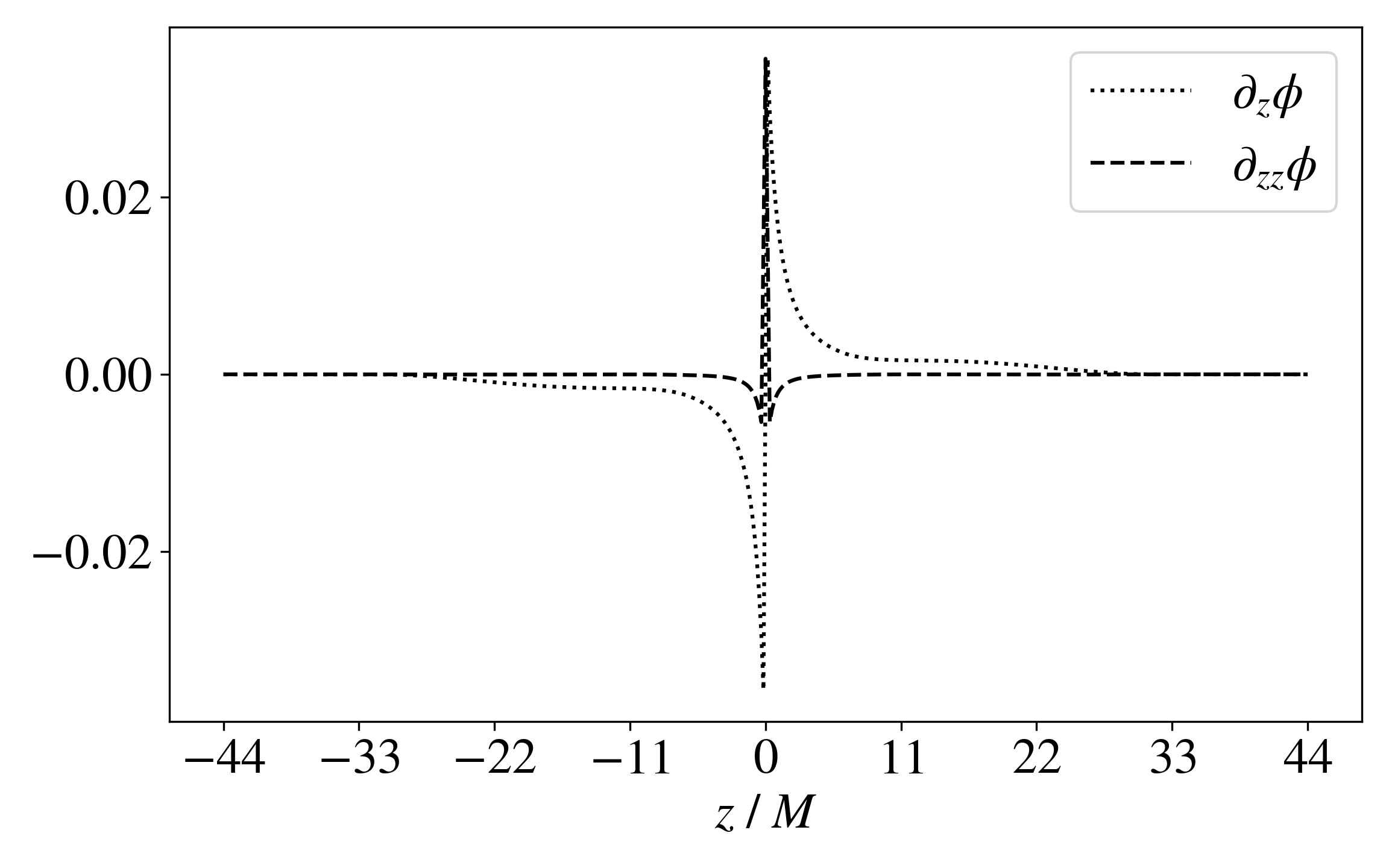
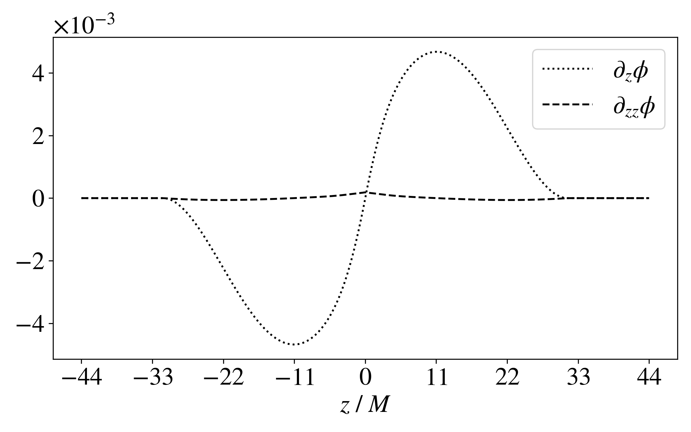
Figure 1: The first and second derivatives of \(\phi\) along the \(z\)-axis for three different potentials. From top to bottom: Gaussian, NFW and Burkert profiles, all corresponding to the strong gravity case with \(\phi_{\text{max}}=0.49\).. a — Derivatives of Gaussian potential, b — Derivatives of NFW potential, c — Derivatives of Burkert potential
Introducing this spline setup means that we are forcing \(\phi\) and its derivatives to vanish at finite \(r\), thus rendering the central overdensity gravitationally “invisible” at
distances \(r\geq r_2\). This requires the introduction of a region with small negative density, here well below the numerical precision of the simulation at \(\sim 10^{-5}\). Although the
negative density is not physical, we introduce it here as a purely numerical approximation and in appendix 7, fig. 10 we show that the deviation of null geodesics due to
the spline is similar to non-spline case and the spline only affects the focusing distance of the GWs.
We initialize the wave at a distance slightly greater than \(r_2\) where \(\phi = 0\). More precisely, we initialize the wave as a wave packet by introducing the wave amplitude \[\mathcal{A_{\text{pw}}} = \left( \frac{1}{1 + e^{-2q(z-l_1)}} + \frac{1}{1 + e^{-2q(l_2 - z)}} -1 \right),\] where \(l_1\) and \(l_2\) are the distances inside
which the wave fronts are confined at initial time. The parameter \(q\) determines how smoothly the wave fronts reach their peak amplitude. For very small \(q\), the wave packet would look
like a Gaussian pulse. For larger values of \(q\), we instead have a square wave function.
Finally, we specify the wave frequency \(k_z\) close to the width of \(\phi(r)\) since this should lead to wave optics effects. For the Gaussian potential, we set \(\lambda = 1.0\) and with that, we define \(k_z = \dfrac{2}{\text{FWHM}(\phi)} \simeq 0.4 \;M^{-1}\) (we chose twice the size of the FWHM-Full Width Half Maximum to make the simulation domain
shorter). For the case of the NFW and Burkert potentials, we ensure that these potentials have the same FWHM as the Gaussian potential. This corresponds to setting \(R_s^{NFW} \simeq 0.98 M\) and \(R_s^{bk} \simeq 2.87 M\). Since the FWHM of all the three potentials are equal, the GW that propagates through them are also given the same initial wavelength. In addition, we emphasize that the wavelength of the GWs should not
be greater than the Schwarzchild radius \(r=2M\), i.e. \(k_z < \frac{1}{2} M^{-1}\). Wavelengths greater than this would lead to diffraction effects [11] which we will study elsewhere. By setting the wavelength less than \(2M\), suppresses the diffraction effects and allows us to
better study the interference of waves due to the curvature gradient itself, while still being in wave optics regime.
Since we propagate the waves along the z-axis, we set up a rectangular-cuboid simulation domain with the longer side being along the z-axis. This setup minimizes the computational cost of our simulations. We have tabulated the simulation parameters in
detail in table 1.
| Simulations | ||||||
|---|---|---|---|---|---|---|
| Gaussian | NFW | Burkert | ||||
| 3D grid | \(128^2_{xy} \times 512_z\) | \(128^2_{xy} \times 512_z\) | \(128^2_{xy} \times 512_z\) | |||
| CFL factor | \(0.5\) | \(0.5\) | \(0.5\) | |||
| FWHM of \(\phi\) | \(\simeq 2.473 \;M\) | \(\simeq 2.473 \;M\) | \(\simeq 2.473 \;M\) | |||
| Scale radius | \(\lambda = 1\) | \(R_s \simeq 0.984\) | \(R_s \simeq 5.742\) | |||
| \(\lambda_{\text{GW}}\) | \(\simeq 2.473 \;M\) | \(\simeq 2.473 \;M\) | \(\simeq 2.473 \;M\) | |||
| \(k_z ^{\text{GW}}\) | \(\simeq 0.404 \;M^{-1}\) | \(\simeq 0.404 \;M^{-1}\) | \(\simeq 0.404 \;M^{-1}\) | |||
3.4 Constraint Damping↩︎
If the gauge conditions are satisfied on the initial Cauchy surface, the constraint violation should in principle be satisfied throughout the evolution [66]. However, when numerically evolving Einstein’s field equation, equation 3 , the numerical precision of the computations lead to growth in the constraint violation over time even when they are
perfectly satisfied initially. This eventually leads to development of unwanted spurious gauge modes. To avoid this, we damp the constraint violations appearing due to this numerical error. We follow the formalism developed by [67] and adopt an approach similar to [68]. We add a term \(- \kappa (t_\alpha Z_\beta + t_\beta Z_\alpha)\) to 4 where \(Z_\alpha \equiv \mathcal{C}_\alpha = \nabla^\mu \bar
h_{\mu \nu}\). Here \(\kappa\) is a positive constant and \(t_\alpha\) is a future pointing timelike vector field. We now choose a simple form of \(\kappa\) and \(t_\alpha\) that would make the addition of this extra term directly proportional to 4 . Hence, we set \(\kappa = 1\) and
\(t_\alpha = -\delta^t_\alpha\). Thus, we add \(\Box_{tt} = 2Z_t\), \(\Box_{tx} = Z_x\), \(\Box_{ty} = Z_y\) and \(\Box_{tz} = Z_z\) to the right-hand-side of the evolution equations.
In appendix 8, we show that constraints converge to zero with higher simulation resolution, supporting that the constraint violations that arise during the evolutions are numerical artifacts due to the numerical
discretisation error and thus do not represent a physical Lorenz gauge violation. In figures 12,13,14,15,16 and 17, we show that the maximum constraint violations are well below the order of magnitude of the GW signal and most of the violation happens due to the wave reflection at the
boundary.
3.5 Adaptive Mesh Refinement (AMR)↩︎
To resolve the features in the waves better, we set up two AMR grids on top of the base grid with one refinement level that has twice the resolution of the base grid. To better resolve \(\phi\) and its derivatives in the
simulation centre, we set up a stationary box-like AMR cuboid with a specific radius to resolve the steep curvature gradients. We set up an another AMR grid on top of the wave packet with a size slightly greater than the wavepacket. We then move this AMR
grid along with the wave as it propagates. At each iteration the AMR grid is moved by calculating the energy weighted centroid along the z-axis given by \[z_{\text{wave-centre}}(t) = \frac{\sum \;z \cdot E(z,t)}{ \sum E(z,t)
}\] where \(E(z,t) = \dfrac{1}{2} u_t^2 + \dfrac{1}{2} \exp(4\phi) (\nabla u)^2\) is the energy of the wave packet along z-axis.
We emphasize that these simulations involve the evolution of all ten components of the GW tensor, together with their associated first and second derivatives, as well as requirement to store the background metric and its derivatives in memory. As a result,
the memory requirements are substantial, and the computations also demand sufficient memory bandwidth. An alternative strategy would be to recompute these quantities each time they appear in the evolution equations, but this would further increase the
computational cost and make the simulations significantly slower. Consequently, performing simulations without adaptive mesh refinement (AMR) becomes extremely expensive and, beyond a certain point, computationally impractical. For simulations of this
kind, adaptive mesh refinement (AMR) is therefore essential. High resolution is required only in the vicinity of the central potential and in the regions occupied by the propagating wave, whereas the rest of the computational domain can be evolved at
comparatively low resolution. This substantially reduces the memory requirements and computational cost, while preserving the accuracy needed in the physically relevant regions.
4 Numerical Results for GW propagation through a Gaussian density distribution↩︎
In this section, we present the simulation results from propagating GWs through a Gaussian density by solving full Einstein equation, \(G_{\mu \nu}=8 \pi T_{\mu\nu}\). We also perform two simulations with \(G_{\mu \nu} = 0\) with Gaussian density and compare it with the simulation evolving full Einstein equation. This helps us distinguish the contributions from the \(T_{\mu \nu}\) part of the Einstein’s equation. In addition, we compare these results with linearly approximated scalar wave equation evolution (equation 6 ).
In the figures we present, we overlay the geodesics on top of our simulation results.
4.1 Gaussian potential: weak gravity regime↩︎
In this subsection, we present the results for GW propagation through a Gaussian potential in the weak gravity regime. Figure 2 shows a two-dimensional slice of the evolution of the \(h_+
= h_{xx}\) component as the wave propagates from left to right through the lens/density distribution. The figure also shows an overlay of null geodesics for the potential configuration (refer to appendix 7
for the details on how we compute the null geodesics), by which we can asses if the wave roughly travel along null geodesics. We present the results in terms of the observable \(h_+\) rather than the trace-reversed metric
perturbation \(\bar{h}_{\mu\nu}\). These two are related by \(h_{\mu \nu} = \bar{h}_{\mu \nu} - \frac{1}{2}\bar{h}\, g^B_{\mu \nu}.\)
The incident plane wave is initially located in a flat Minkowski region, where \(\phi = 0\), on the negative \(z\)-axis and \(\partial_t h_+\) is set such
that the wave propagates from negative to positive \(z\). The wave’s initial peak amplitude is normalized to unity. Figure 2 displays the wave profile at two representative times:
shortly after the wave has passed through the central density at \(t = 45.63\,M\), and after it has completely exited the curved region, at \(t = 65.91\,M\). At \(t
= 45.63\,M\), the portion of the wave near \(x=0\) lags behind the wavefront near the outer boundaries. This is the well-known Shapiro time delay [69]. At the same time, the amplitude in the central region is enhanced due to gravitational focusing; in the language of wave optics, this enhancement arises from constructive interference of
the wave with itself.
The figure also includes the quantity \(|h_+ - h_+^{\text{simplified}}|\), where \(h_+^{\text{simplified}}\) denotes the solution of the simplified wave equation defined in equation 6 . This comparison allows us to isolate the effects of the additional geometric terms involving the Christoffel symbols and the Riemann curvature tensor that appear in the full Einstein equations. The difference is of order
\(10^{-2}\), and the corresponding plot shows that a small “tail” like structure behind the wavefronts near \(z=4 \;M\) when we solve the full equations.
At the later time \(t = 65.91\,M\), the plot of \(|h_+ - h_+^{\text{simplified}}|\) now shows a characteristic pattern with a maximum amplitude of order \(10^{-2}\). Here, we note that the interference pattern in the longitudinal direction is a numerical artifact of the reflecting boundary conditions. We do not expect that this pattern represents a physical effect.
In figure 3 (top figure), we show the difference between the simulations evolving the full Einstein equation versus the density-free equations (indicated as \(h_+^{\text{(no
density)}}\) in the figure). From this comparison, we see that a very weak amplitude of GW is scattered in almost all directions by the density field. Again, we included an overlay of null geodesics trajectories on top of the two-dimensional slice
to show that this behaviour is not predicted by the null geodesic description of wave propagation. This is seen by parts of the wave fronts moving in directions that are clearly not orthogonal to the geodesics. Although this effect is interesting in
itself, its smallness in amplitude indicates that the results we obtain for the other density profiles are reasonably accurate for weak gravity case despite only studying the density-free equations.
Figure 4 (a) shows the evolution of the maximum amplitude of \(h_+\) and \(|h_+^{\text{simplified}}|\), tracked along \((x,y)=(0,0)\). As expected from focusing, the amplitude increases as the wave traverses the curved region. The corresponding null geodesic overlay in Fig. 2 shows that the strongest
convergence of the ray bundle occurs at a distance of approximately \(z = 40\,M\) from the peak of the potential. A noticeable difference develops between \(h_+\) and \(h_+^{\text{simplified}}\) when the wave passes through the central density. However, their final amplitudes remain similar, differing only at the level of \(10^{-2}\), consistent with the
behaviour seen in Fig. 2.
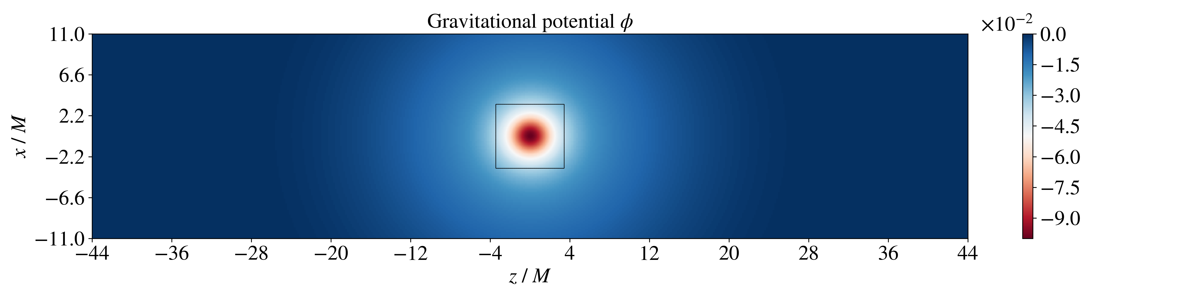
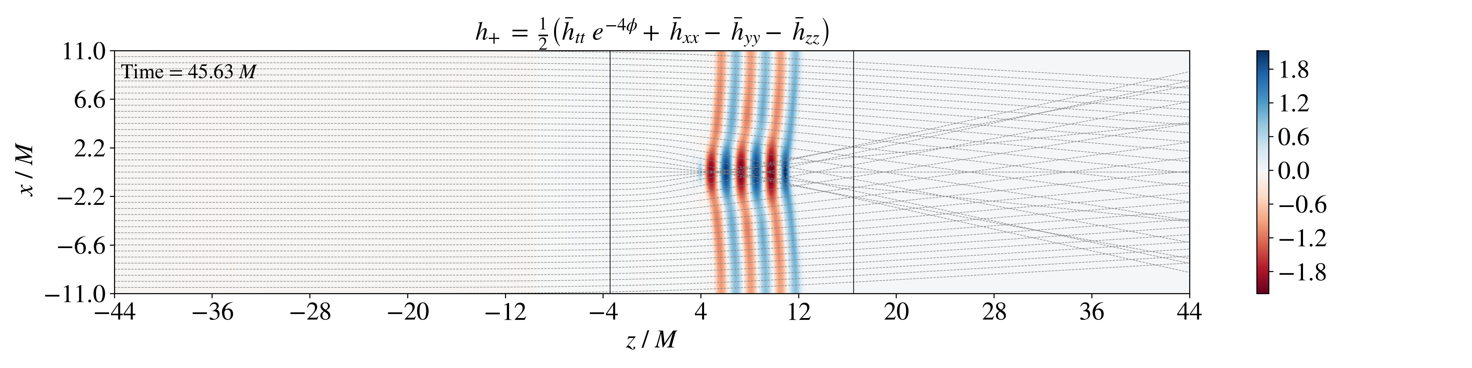
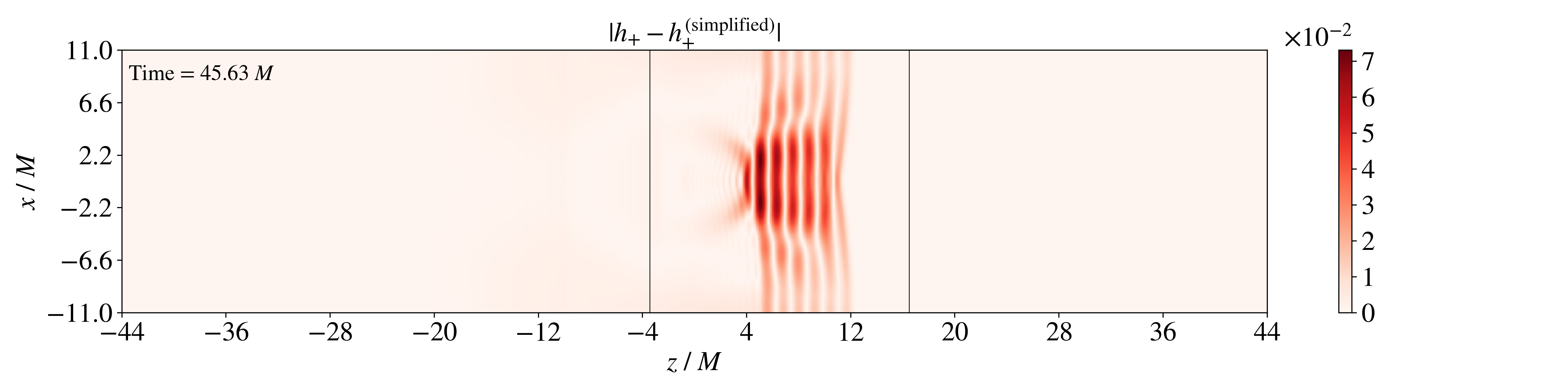
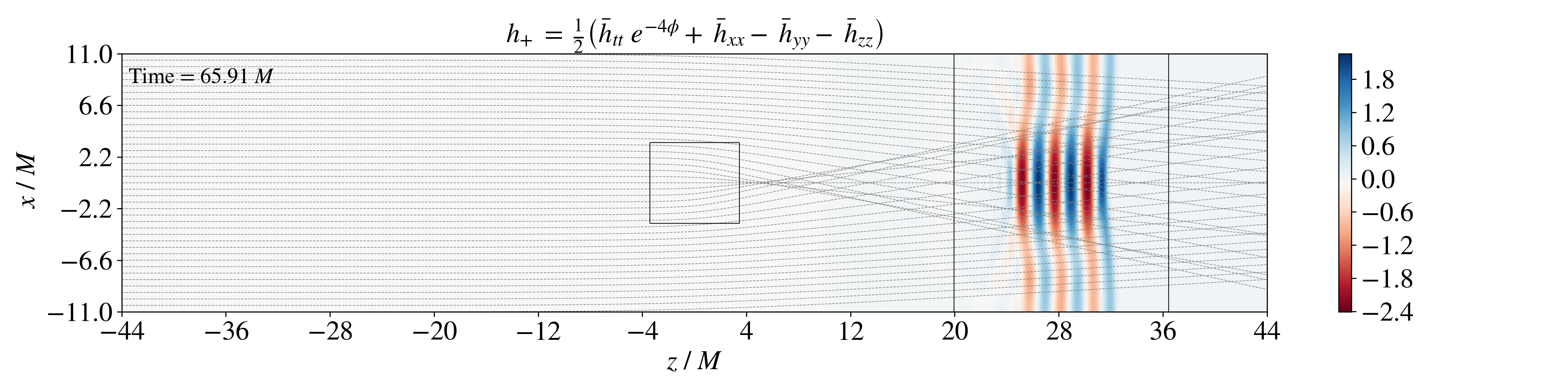
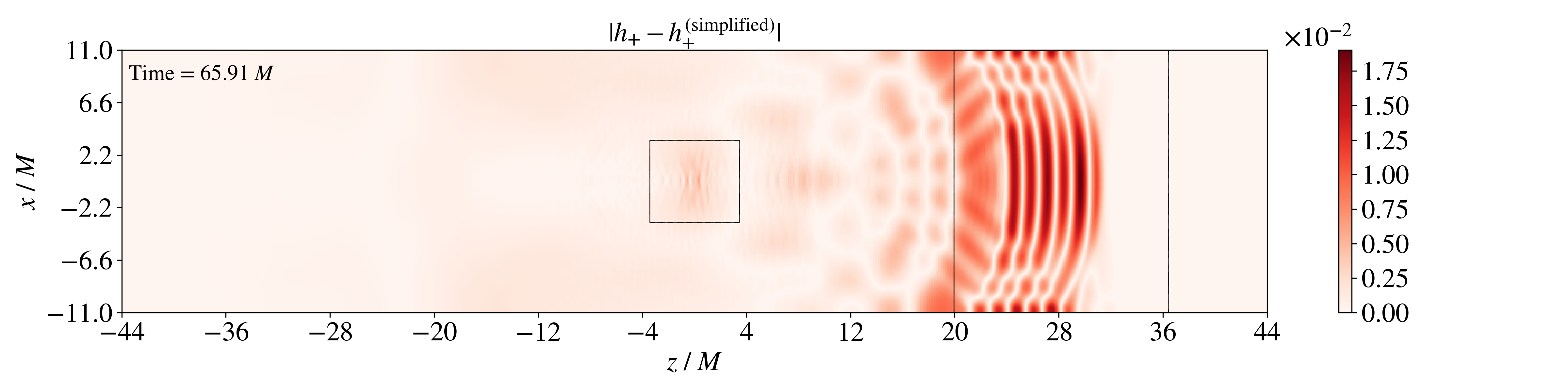
Figure 2: From top to bottom: Top figure shows the distribution of gravitational potential \(\phi\) along \(x-z\) axis for Gaussian potential in weak gravity regime. The second figure shows the 2D slice of \(h_+\) after the wave has traversed the central density at \(t=45.63 \;M\). Third figure shows the absolute difference between \(h_+\) and \(|h_+^{\text{simplified}}|\) which are evolved independently with the same initial conditions, that helps in distinguishing the effects arising from terms that are purely geometric. Fourth and fifth figure shows the wave after it has completely exited the curvature at a later time \(t=65.91 \;M\). The figure for \(h_+\) has an overlay of null geodesics for the potential configuration considered with spline. The black outlined boxes inside the simulation domain is where the AMR patch exists and has twice the resolution of base grid..
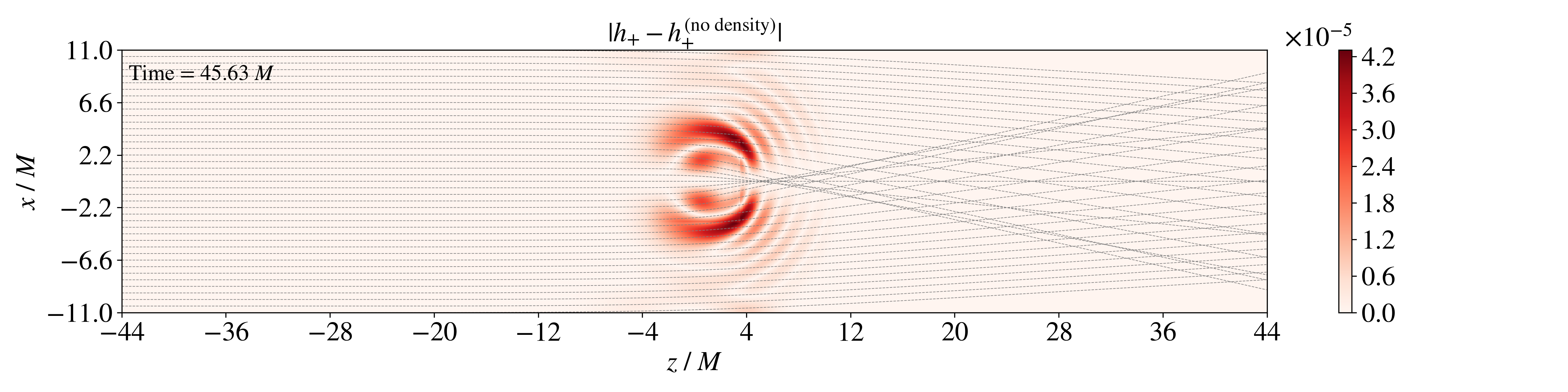
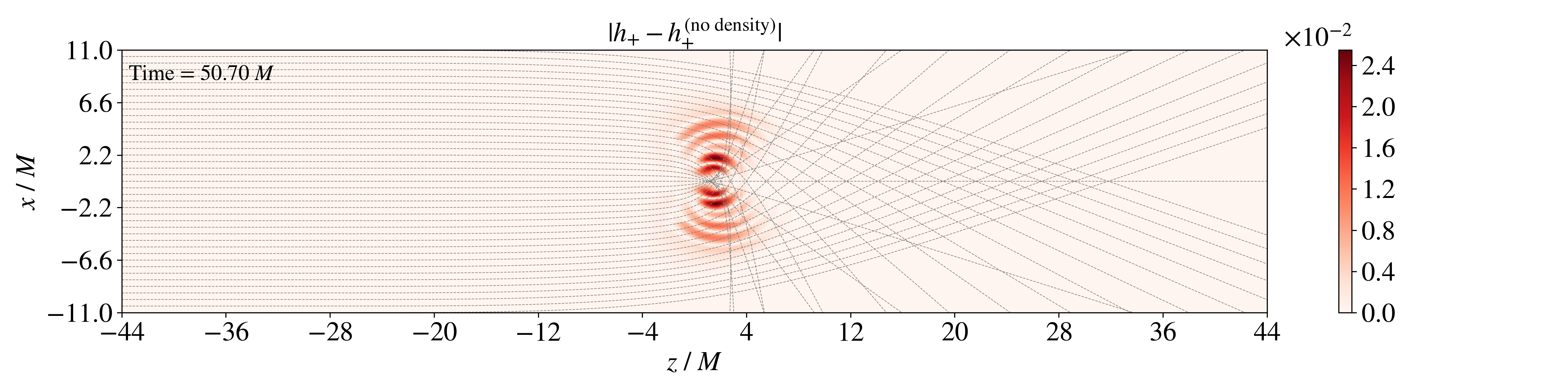
Figure 3: The top and bottom panels of Fig. 3 show the difference between the two evolutions considered, namely the full Einstein-equation evolution and the vacuum evolution with \(G_{\mu\nu}=0\), for the Gaussian density in the weak and strong gravity regimes, respectively, at the instant when the GW is traversing the density distribution. The plots also include an overlay of the corresponding null geodesics(with spline), shown as gray dashed lines, for both gravity regimes. We find that the difference between the two solutions is extremely small (order of \(10^{-5}\)) in the weak gravity case, whereas in the strong gravity case it reaches the level of a few percent of the overall GW signal..
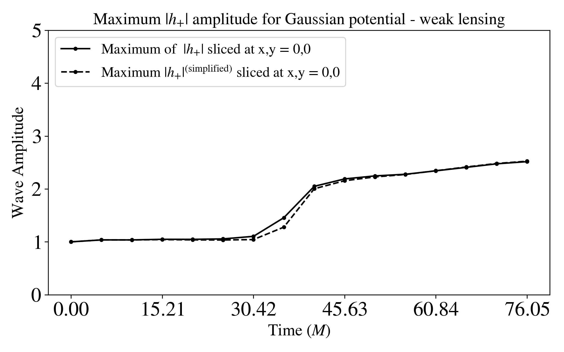
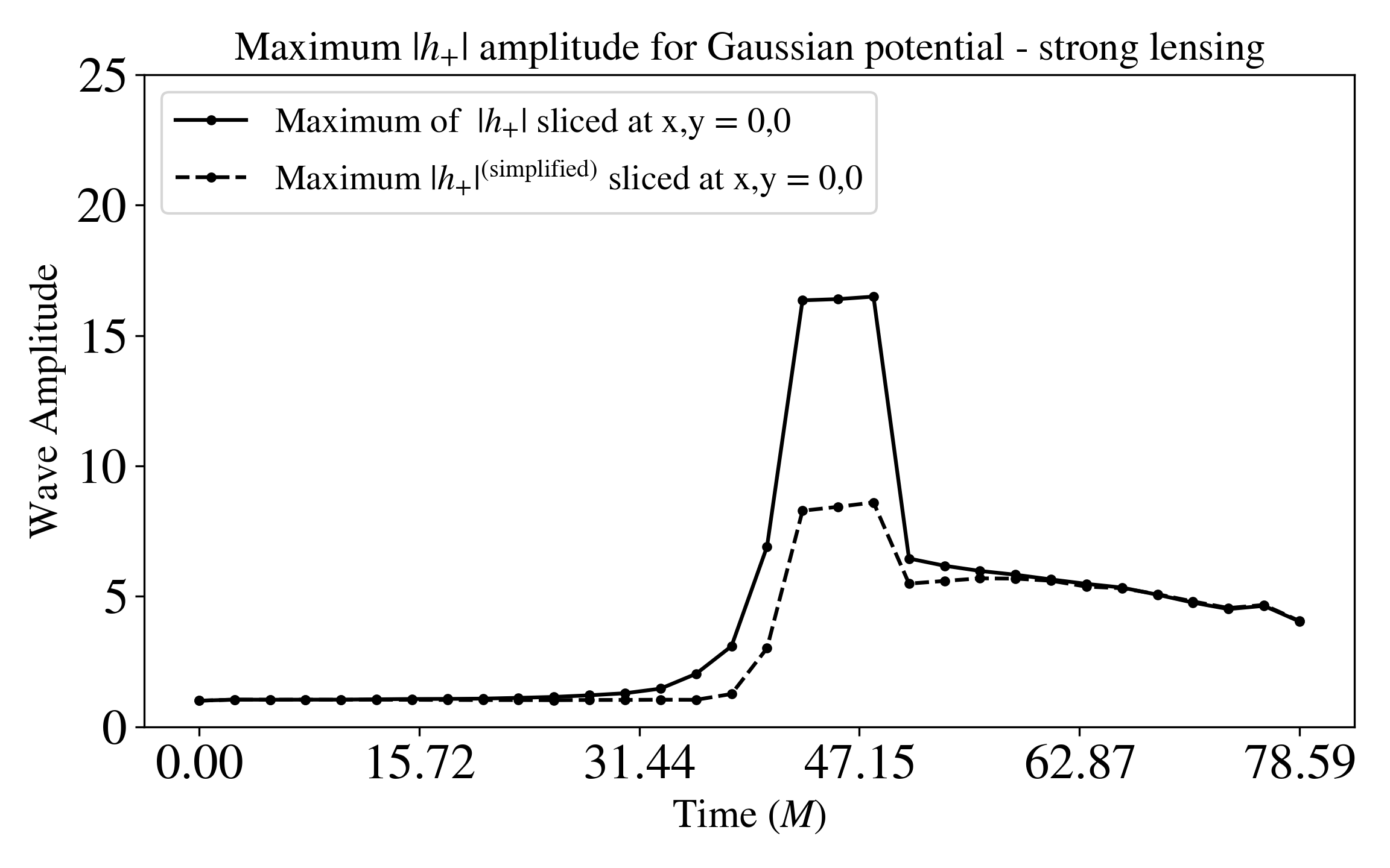
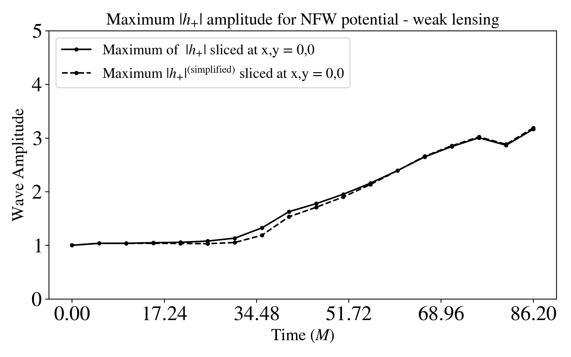
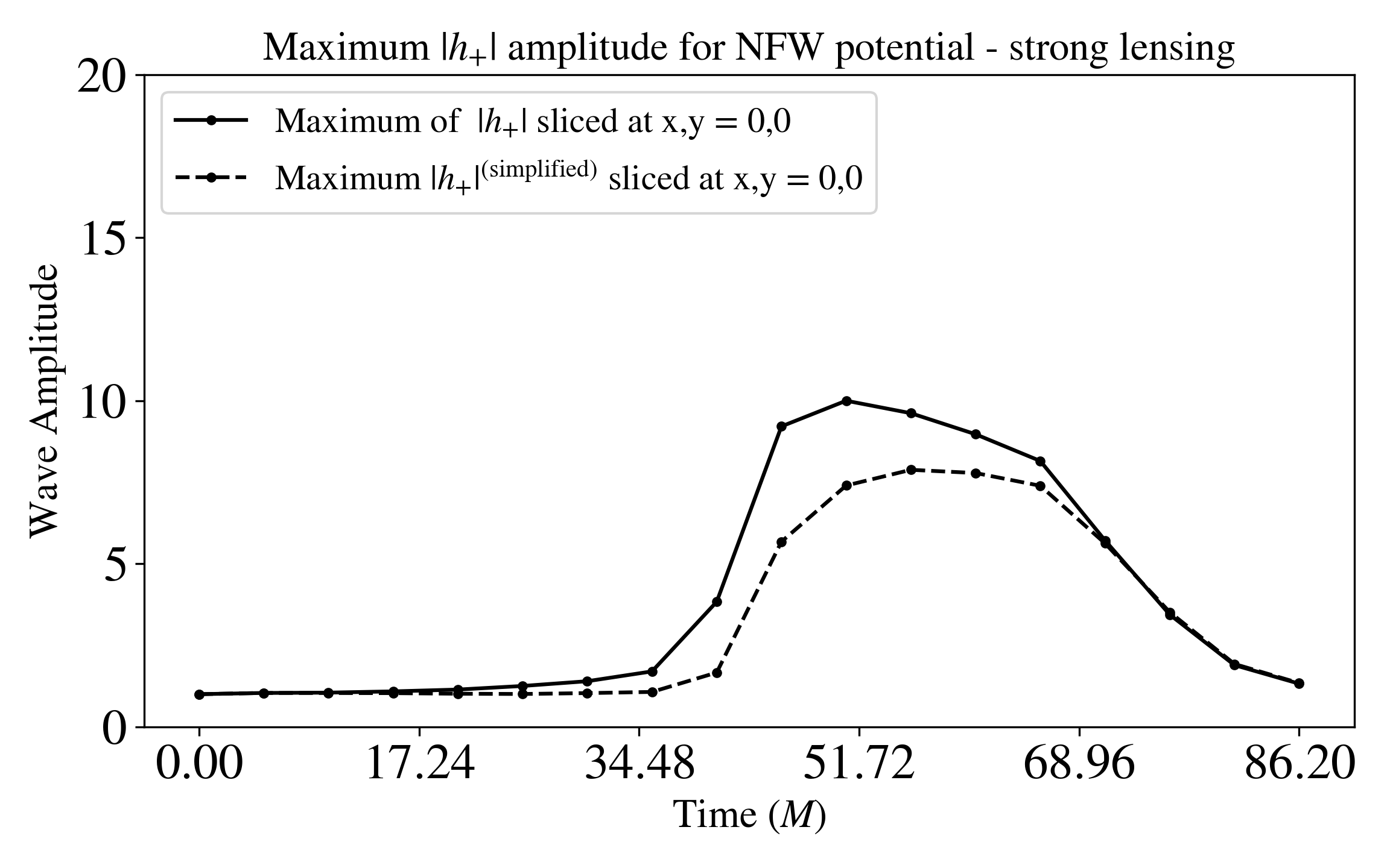
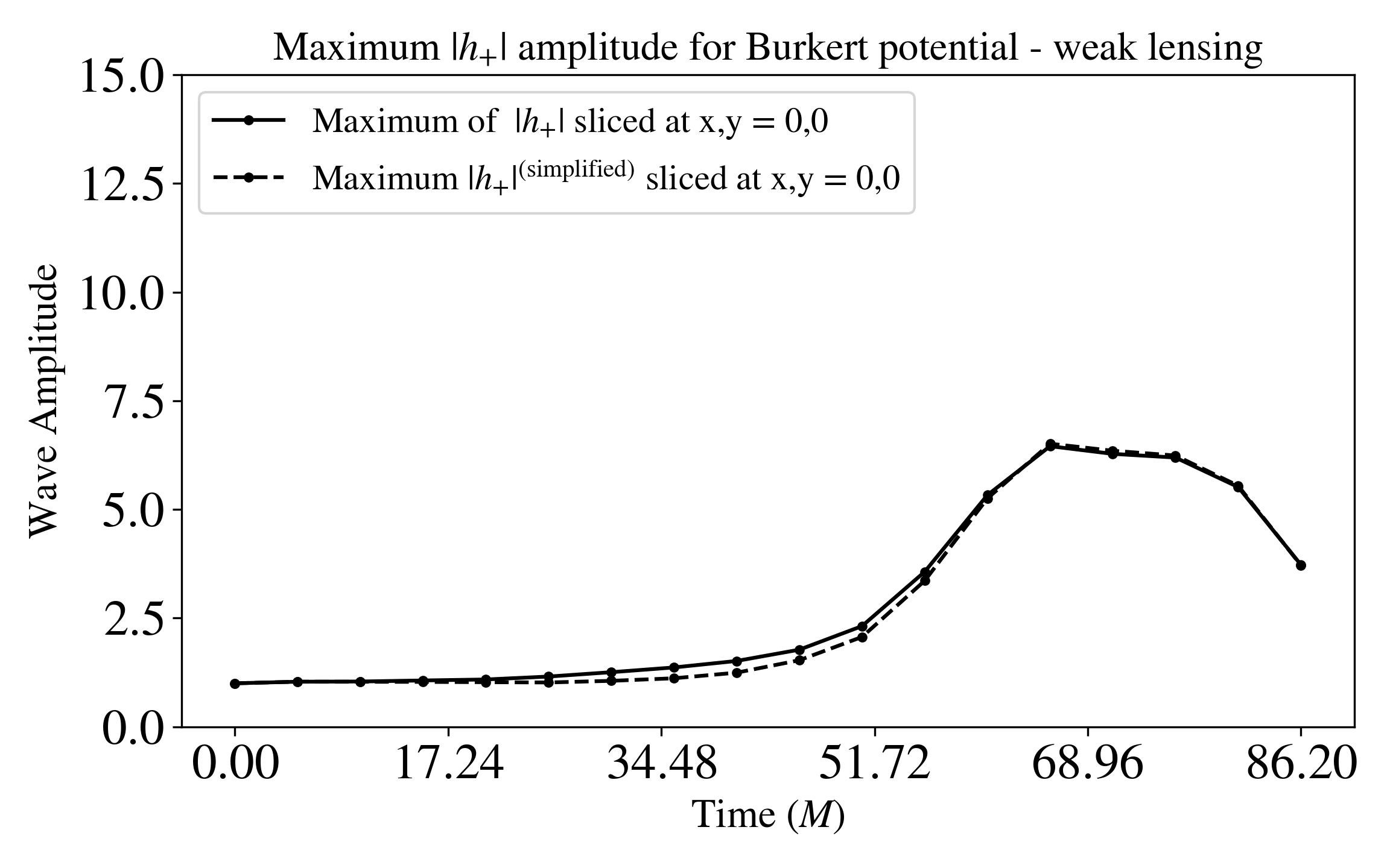
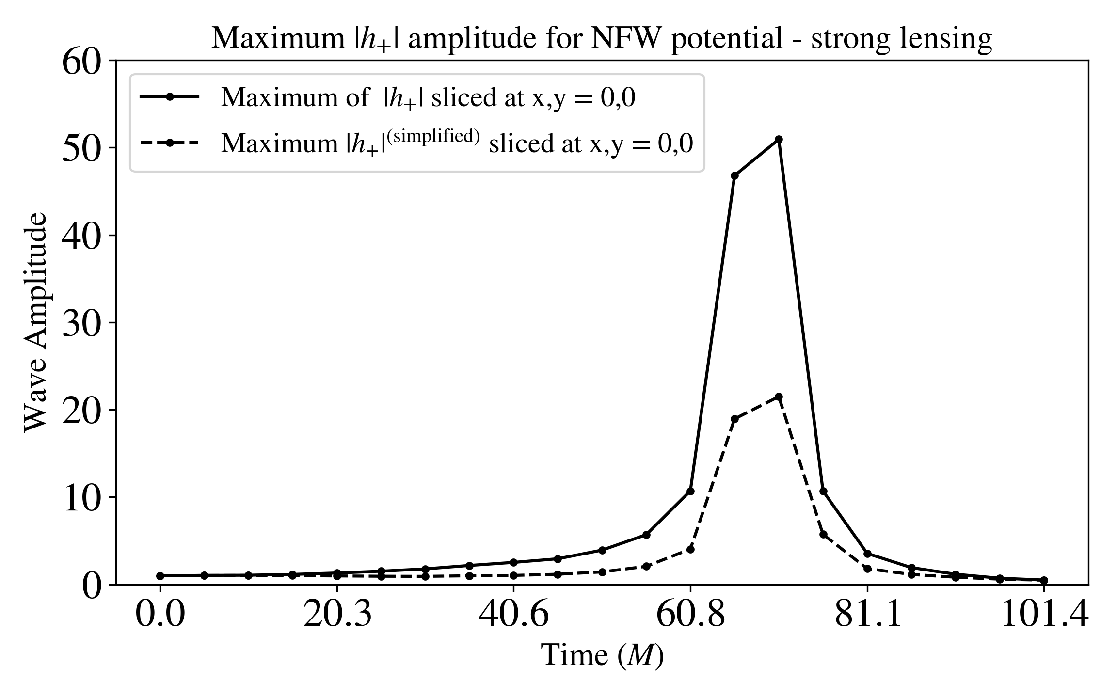
Figure 4: Figure shows the evolution of the maximum amplitude of the \(h_+\) and \(|h_+^{\text{simplified}}|\) waves, sampled at \((x,y)=(0,0)\), for the Gaussian, NFW, and Burkert potentials in both the weak and strong gravity regimes. In all cases, the maximum amplitude increases during the evolution as a result of gravitational focusing. Among the weak gravity configurations, the Gaussian potential produces the smallest amplification. This is consistent with the corresponding null geodesic structure shown in Fig. 10 (a), where the region over which the ray bundle intersects is the most extended, leading to weaker concentration of the wave energy. In contrast, the Burkert potential in the strong gravity regime yields the largest amplification. As seen in Fig. 10 (f), the ray bundles intersect within a much smaller region, resulting in stronger focusing and hence a larger peak amplitude.. a — Maximum wave amplitude of \(h_+\) and \(|h_+^{\text{simplified}}|\) - Gaussian potential, weak gravity case, b — Maximum wave amplitude of \(h_+\) and \(|h_+^{\text{simplified}}|\) - Gaussian potential, strong gravity case, c — Maximum wave amplitude of \(h_+\) and \(|h_+^{\text{simplified}}|\) - NFW potential, weak gravity case, d — Maximum wave amplitude of \(h_+\) and \(|h_+^{\text{simplified}}|\) - NFW potential, strong gravity case, e — Maximum wave amplitude of \(h_+\) and \(|h_+^{\text{simplified}}|\) - Burkert potential, weak gravity case, f — Maximum wave amplitude of \(h_+\) and \(|h_+^{\text{simplified}}|\) - Burkert potential, strong gravity case
4.2 Gaussian potential: strong gravity regime↩︎
In this subsection, we present the results for GW propagation through a Gaussian potential in the strong gravity regime, corresponding to \(\phi_{\mathrm{max}} = -0.49\). Figure 5
shows a two-dimensional slice of the evolution of the \(h_+\) component as the wave propagates from left to right through the lens. The figure also shows an overlay of null geodesics for the potential configuration.
As before, the incident plane wave is initially located in a flat Minkowski region on the negative \(z\)-axis and propagates toward positive \(z\). Its initial peak amplitude is normalized
to unity. Figure 5 displays the wave profile at two representative times: first, shortly after the wave has passed through the central density, at \(t = 55.77\,M\), and second, after
it has completely exited the curved region, at \(t = 76.05\,M\). At \(t = 55.77\,M\), the portion of the wave near \(x=0\) exhibits a pronounced Shapiro time
delay. In addition, the wave amplitude in the central region is significantly enhanced by strong gravitational focusing. The figure also shows that the wave develops a distinct “tail” produced by the large curvature near the lens. This appears because
waves originating from the upper part of the \(x\)-axis are deflected downward, while those from the lower part are deflected upward. This feature is therefore much more pronounced than in the weak gravity case. The
corresponding plot of \(|h_+ - h_+^{\text{simplified}}|\) shows differences of order \(10^{-1}\). It also reveals that, in the region surrounding the density peak, part of the wave is
scattered in multiple directions with prominent amplitude in the direction orthogonal to the initial direction of propagation. Parts of these scattered waves do not seem to propagate orthogonally to any null geodesics. This is also seen in Fig. 3 (bottom figure), where we plot the difference between simulations solving the full Einstein equation vs. the density-free equation (represented as \(h_+^{\text{(no density)}}\)).
Here, we see that an amplitude of a few percent of the total GW signal is scattered in almost all directions, similar to the weak gravity case but with much stronger amplitude. This behaviour is not predicted by the null geodesic description of wave
propagation. We therefore find that the wave dynamics exhibit a few percentage deviation from the null geodesic approximation when the wave propagates through the density distribution. This indicate that, for sensitive GW observations, the effects
associated with the full Einstein equations are relevant and should be incorporated into accurate signal modelling. Nonetheless, the density-free approximation captures most of the wave dynamics.
At the later time \(t = 76.05\,M\), after the wave has exited the curved region, its amplitude is slightly reduced compared to the earlier snapshot. This shows that wave amplification does not necessarily persist at all
stages of lensing in the wave-optics regime. In the \(|h_+ - h_+^{\text{simplified}}|\) plot, the portion of the wave in the range \(28 \leq z \leq 40\) exhibits differences with a maximum
amplitude of order \(10^{-2}\). Thus, despite the strong gravity setting, the final magnitude of the difference is comparable to that found in the weak gravity case. This is, however, only true along the principal axis.
Overall, the wave is now significantly more focused than in the weak gravity example.
As for the weak gravity simulation, the imposed reflection symmetry about the \(x\)-axis causes part of the waves seen at \(t = 55.77\,M\) to be reflected back into the computational domain
from both of the \(x\) axis boundaries. The resulting interference pattern across the domain is therefore a numerical artifact of the reflecting boundary conditions rather than a physical effect.
Figure 4 (b) shows the evolution of the maximum amplitude of \(h_+\) and \(|h_+^{\text{simplified}}|\) tracked along the principal axis (the \(z\)-axis). By comparing with Fig. 5, we see that the strongest amplification occurs in the region where the null geodesics converge and overlap significantly. Once the wave has passed
through this region of overlapping geodesics, the amplitude decreases. Although a substantial deviation develops between \(h_+\) and \(h_+^{\text{simplified}}\) while the wave is in the
central density, their final amplitudes are again similar and differ only at the level of \(10^{-2}\), consistent with the behaviour shown in Fig. 5.
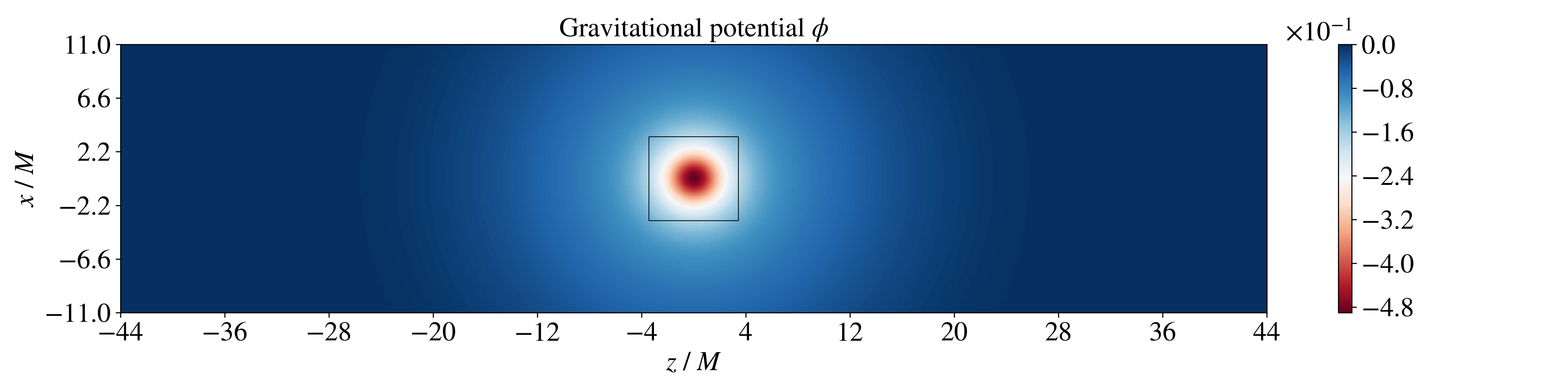
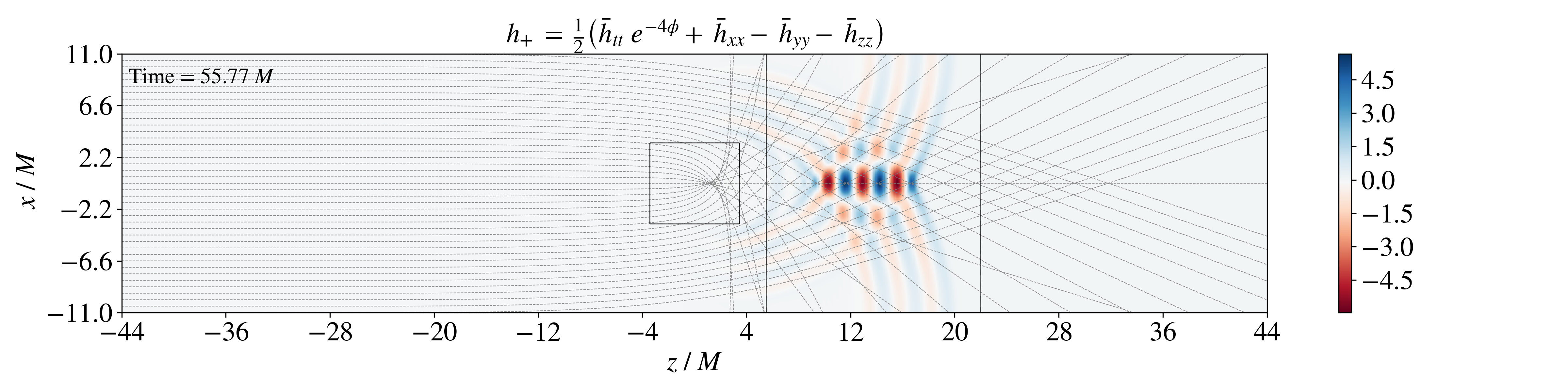
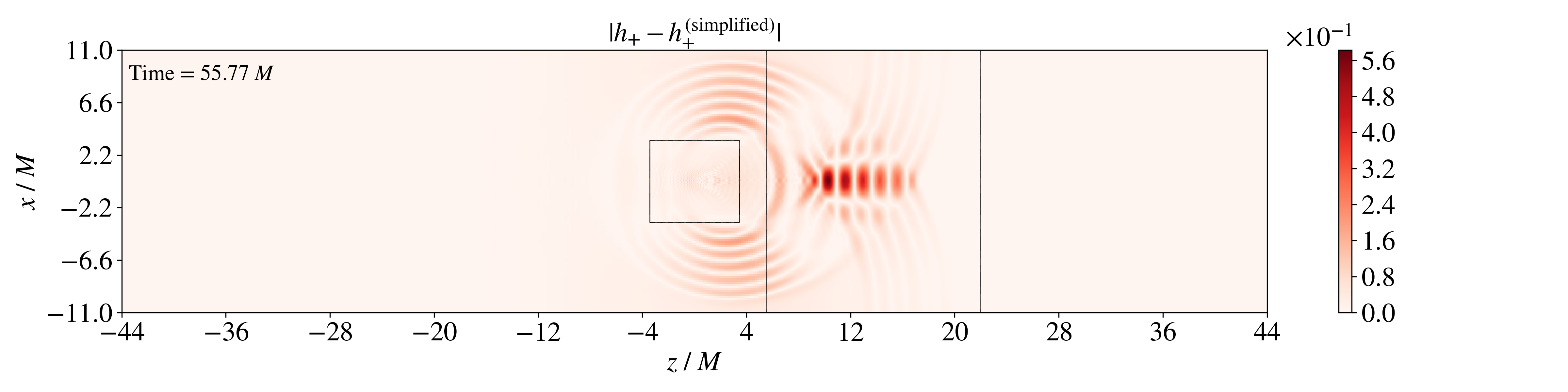

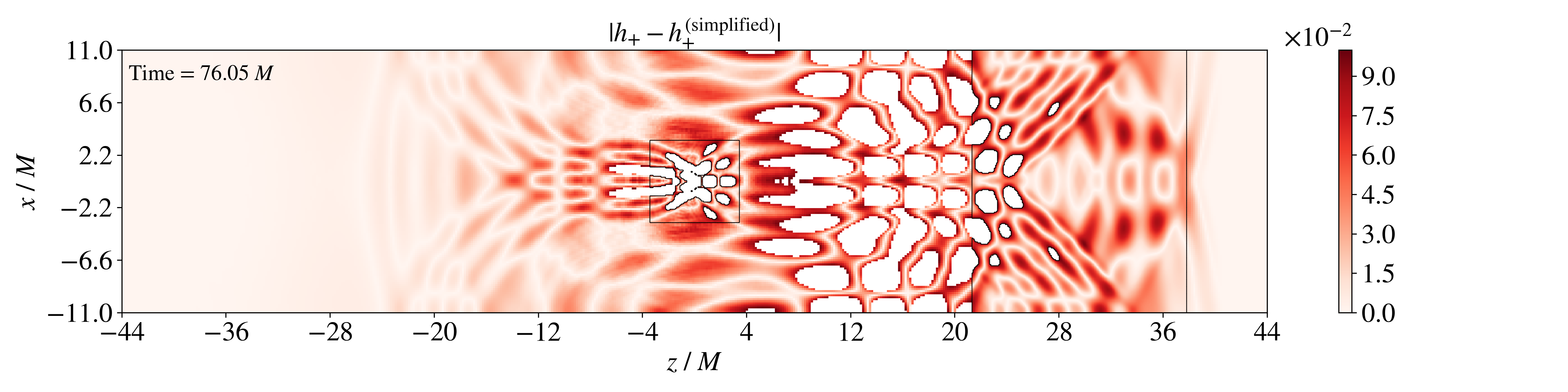
Figure 5: From top to bottom: Top figure shows the distribution of gravitational potential \(\phi\) along \(x-z\) axis for Gaussian potential in strong gravity regime. The second figure shows the 2D slice of \(h_+\) after the wave has traversed the central density at \(t=55.77 \;M\). Third figure shows the absolute difference between \(h_+\) and \(|h_+^{\text{simplified}}|\) which are evolved independently with the same initial conditions, that helps in distinguishing the effects arising from terms that are purely geometric. Fourth and fifth figure shows the wave after it had completely exited the curvature at a later time \(t=76.05 \;M\). The figure for \(h_+\) has an overlay of null geodesics for the potential configuration considered with spline. The regions that are masked white denote region out of bound values of the scale on the right. The black outlined boxes inside the simulation domain is where the AMR patch exists and has twice the resolution of base grid..
5 Numerical results for solution of \(G_{\mu \nu}=0\) for NFW and Burkert profiles↩︎
In this section, we present the results from propagating GWs through NFW and Burkert gravitational potential, by solving the equation \(G_{\mu \nu}=0\). For each potential configuration, we also overlay the corresponding
null geodesics on the simulation results in order to clarify the geometric interpretation of the wave propagation. In addition, we compare these results with those obtained from the linearly approximated scalar wave equation given in Eq. 6 . We remind the reader that we here set \(\rho = 0\) to avoid numerical issues with the diverging densities near the origin. Our results from the previous section suggest that we should
expect this only changes our final results by a few percent compared to if we retained \(\rho\) and e.g. excise or replace it with a numerical scheme to handle the divergence in the centre. We will comment further on this
below.
We start by presenting the result sobtained with the NFW potential.
5.1 NFW potential: weak gravity regime (with \(T_{\mu \nu}=0\))↩︎
In this subsection, we present the results for GW propagation through the NFW potential in the weak gravity regime with the right-hand side of the Einstein equations set to zero, \(T_{\mu \nu}=0\). Figure 6 shows a two-dimensional slice of the evolution of the \(h_+ = h_{xx}\) component as the wave propagates from left to right through the lens.
As in the Gaussian case, the incident plane wave is initially located in a flat Minkowski region on the negative \(z\)-axis and propagates toward positive \(z\). Figure 6 displays the wave profile at two representative times: shortly after the wave has passed through the central potential region, at \(t=50.70\,M\), and after it has completely exited the
curved region, at \(t=76.05\,M\). At \(t=50.70\,M\), the portion of the wave near \(x=0\) is delayed relative to the outer parts of the wavefront, indicating
the expected Shapiro time delay. Additionally, the amplitude in the central region is enhanced due to gravitational focusing. In the plot of \(|h_+ - h_+^{\text{simplified}}|\), the difference is of order \(10^{-2}\). At the later time \(t=76.05\,M\), after the wave has exited the curved region, its amplitude has increased further. The overall wave pattern is qualitatively similar to that found in
the weak gravity Gaussian case. In the plot of \(|h_+ - h_+^{\text{simplified}}|\) a more pronounced interference pattern is visible than in the Gaussian case, although the magnitude of the difference remains at the same
order. As before, reflections occur on the boundaries of the simulation along the \(x\)-axis, causing part of the wave to re-enter the computational domain in the longitudinal direction. The resulting interference pattern
is therefore a numerical artifact of the boundary conditions rather than a physical effect.
Figure 4 (c) shows the evolution of the maximum amplitude of the waves \(h_+\) and \(|h_+^{\text{simplified}}|\), tracked along the principal axis. The
corresponding null geodesics overlayed in Fig. 6 show that the strongest convergence of the ray bundle occurs at \(z \gtrsim 44\,M\). This explains why the wave amplitude continues to
increase even after the wave has passed through the central potential region. The geodesic overlay further suggest that the wave propagation roughly follows the expected null geodesic structure. Although a small difference develops between \(h_+\) and \(h_+^{\text{simplified}}\) during the evolution, their final amplitudes remain very similar and differ only at the level of \(10^{-2}\) as shown in
Fig. 6.
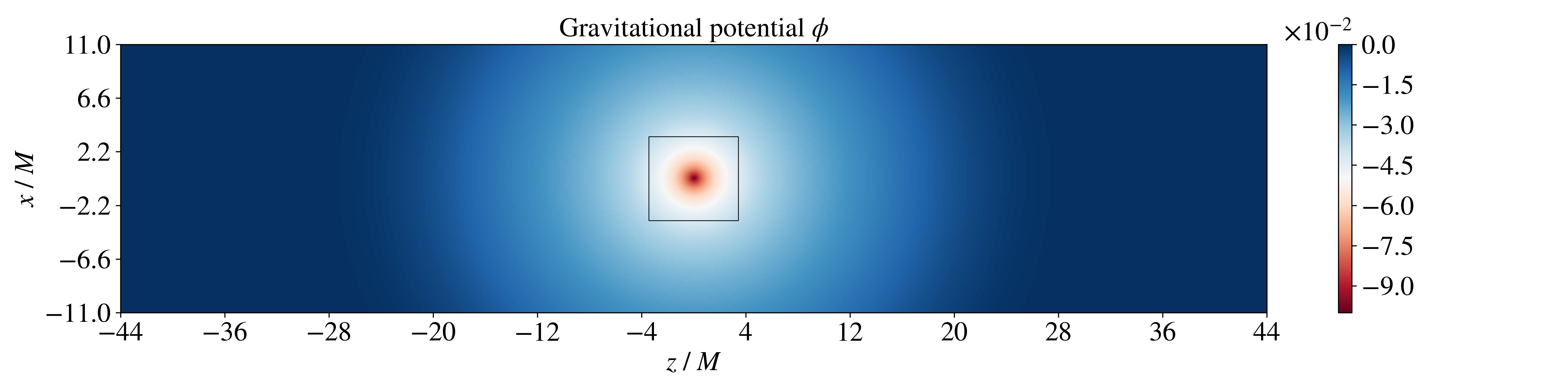
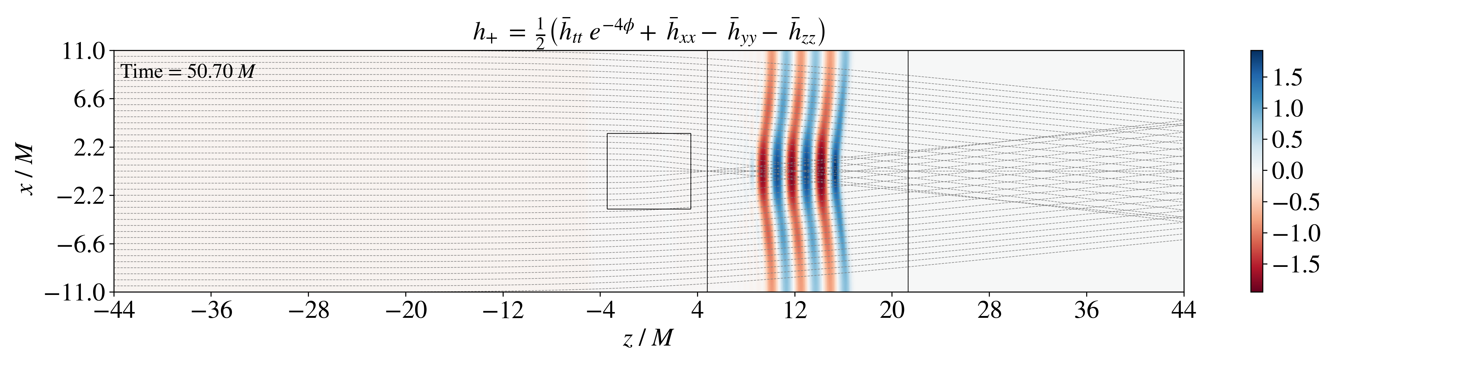
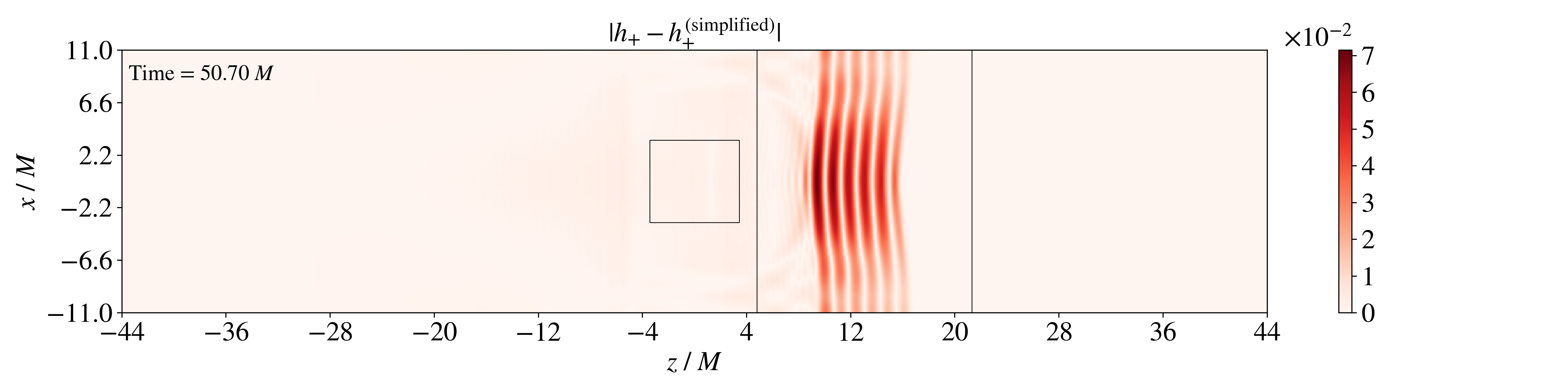
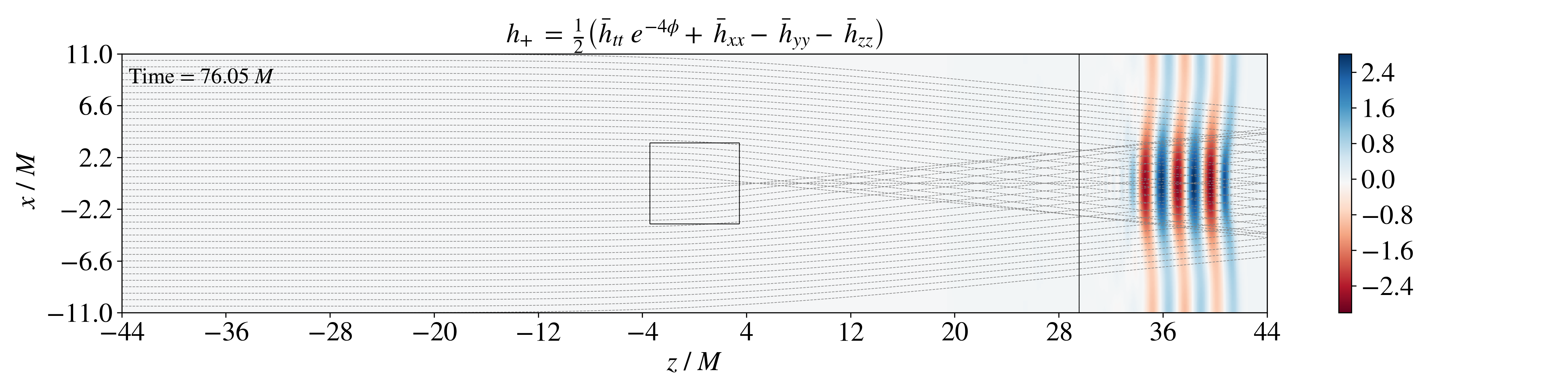
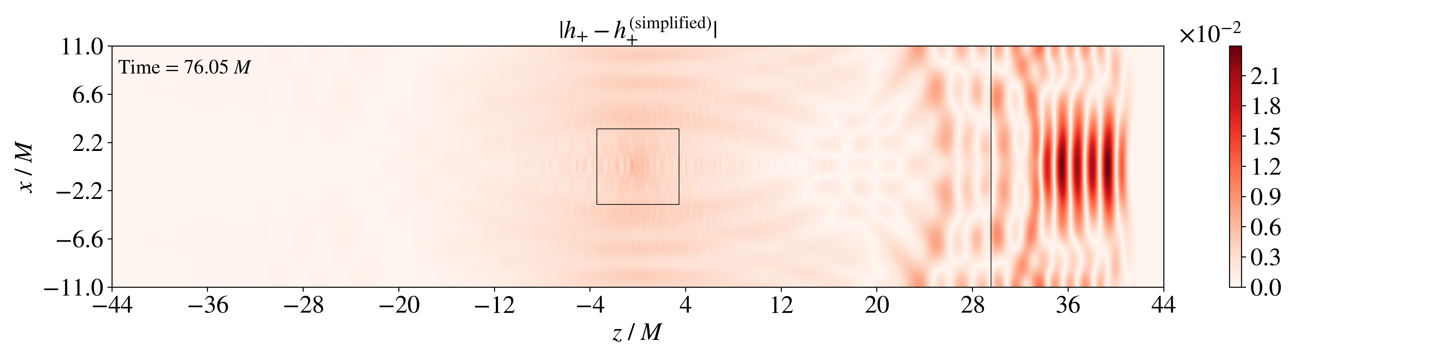
Figure 6: From top to bottom: Top figure shows the distribution of gravitational potential \(\phi\) along \(x-z\) axis for NFW potential in weak gravity regime with \(T_{\mu \nu} = 0\). The second figure shows the 2D slice of \(h_+\) after the wave has traversed the central density at \(t=50.70 \;M\). Third figure shows the absolute difference between \(h_+\) and \(|h_+^{\text{simplified}}|\) which are evolved independently with the same initial conditions, that helps in distinguishing the effects arising from terms that are purely geometric. Fourth and fifth figure shows the wave after it had completely exited the curvature at a later time \(t=76.05 \;M\). The figure for \(h_+\) has an overlay of null geodesics for the potential configuration considered with spline. The black outlined boxes inside the simulation domain is where the AMR patch exists and has twice the resolution of base grid..
5.2 NFW potential: strong gravity regime (with \(T_{\mu \nu}=0\))↩︎
In this subsection, we present the results for GW propagation through the NFW potential in the strong gravity regime, corresponding to \(\phi_{\mathrm{max}} = -0.49\), with \(T_{\mu
\nu}=0\). Figure 7 shows a two-dimensional slice of the evolution of the \(h_+\) component as the wave propagates from left to right through the lens. The results are presented in
terms of the observable \(h_+\).
As in the earlier simulations, the incident plane wave is initially located in a flat Minkowski region on the negative \(z\)-axis and propagates toward positive \(z\)-axis. Figure 7 displays the wave profile at two representative times: shortly after the wave has passed through the central potential region, at \(t=55.77\,M\), after it has completely exited the curved
region, at \(t=81.12\,M\).
At \(t=55.77\,M\), the waves in the central region exhibit a substantial increase in amplitude due to strong gravitational focusing. In addition, the wave develops a pronounced “tail” structure, caused by the strong
curvature, which mixes the upper and lower parts of the wavefront. The corresponding plot of \(|h_+ - h_+^{\text{simplified}}|\) shows that the difference is of the same order of magnitude as the GW signal itself,
indicating that the simplified wave equation fails to capture important features of the evolution in this regime. This is again very similar to the Gaussian case, although with a distinctly different interference pattern.
At the later time \(t=81.12\,M\), after the wave has exited the curved region, its amplitude has decreased significantly relative to the earlier snapshot. This indicates that the amplification did not persist throughout the
evolution. Owing to the strong bending induced by the curvature, parts of the wave are reflected from the \(x\)-axis boundaries and re-enter the computational domain. In the plot of \(|h_+ -
h_+^{\text{simplified}}|\), the portion of the wave in the range \(32 \leq z \leq 40\) shows a maximum difference of order \(10^{-2}\). Thus, despite the strong gravity setting, the
final discrepancy in this region is comparable in magnitude to that found in the weak gravity case, which is \(10^{-2}\).
Figure 4 (d) shows the evolution of the maximum amplitude of the waves \(h_+\) and \(|h_+^{\text{simplified}}|\), tracked along the principle axis. The
strongest amplification occurs in the region where the null geodesics exhibit the greatest overlap, as shown in Fig. 7 overlay, namely for \(0<z<20\). After the wave has traversed
this region, the amplitude decreases. This behaviour is consistent with the interpretation that the wavefront propagates along directions determined by the null geodesic structure. Although a substantial difference develops between \(h_+\) and \(h_+^{\text{simplified}}\) while the wave passes through the central potential region, their final amplitudes again become similar and differ only at the level of \(10^{-2}\), as seen in Fig. 7.
Overall, the results obtained with the Gaussian and NFW profiles are quantitatively very similar, but qualitatively they differ in their exact interference patterns.
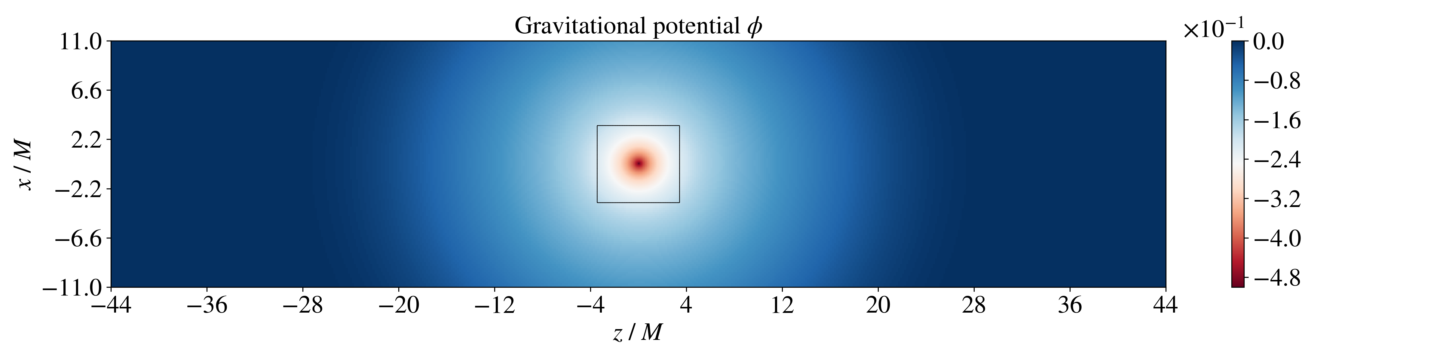
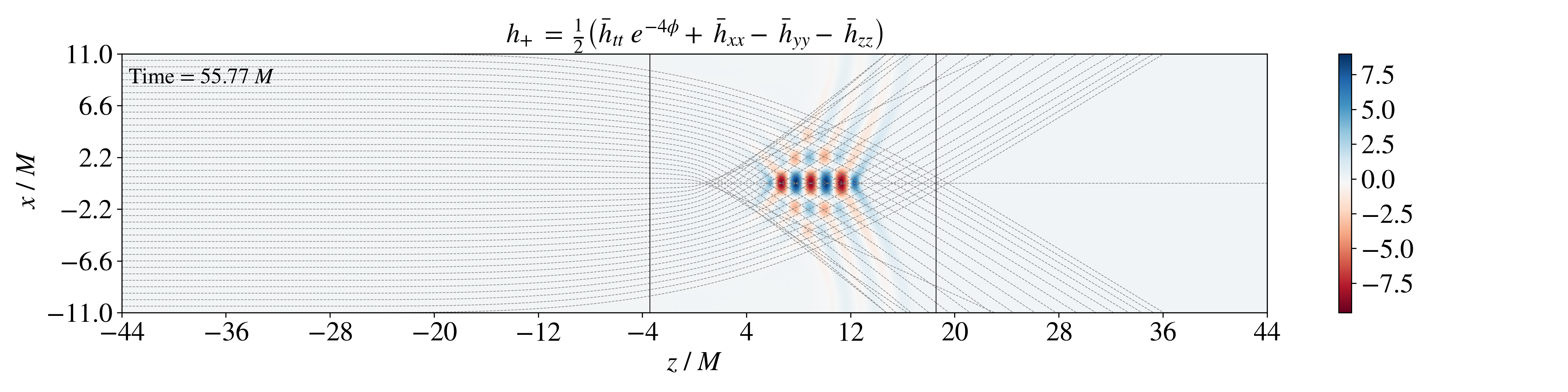
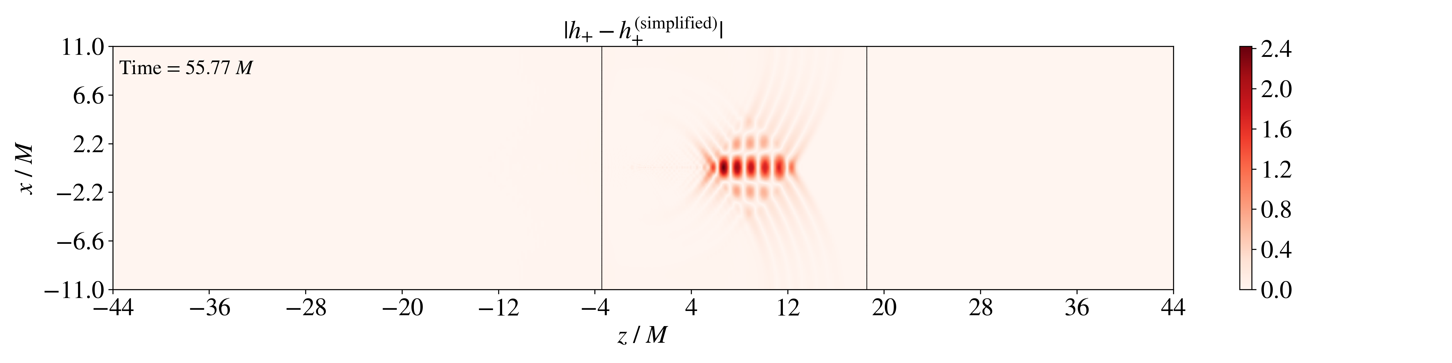
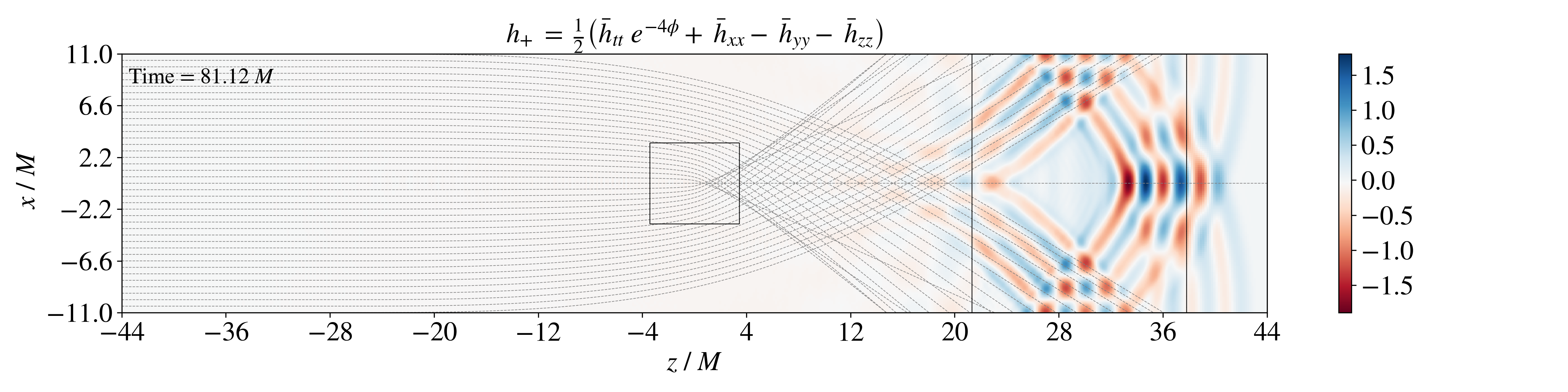
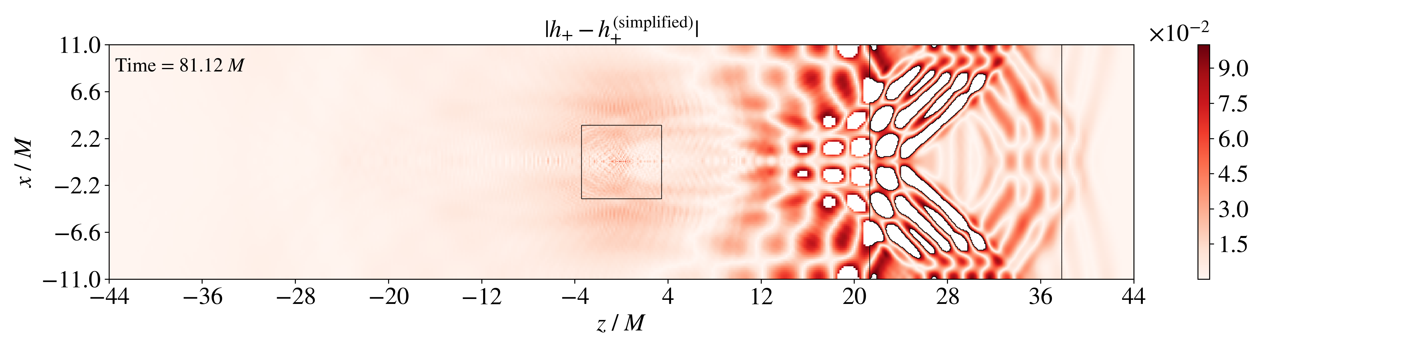
Figure 7: From top to bottom: Top figure shows the distribution of gravitational potential \(\phi\) along \(x-z\) axis for NFW potential in strong gravity regime. The second figure shows the 2D slice of \(h_+\) after the wave has traversed the central density at \(t=55.77 \;M\). Third figure shows the absolute difference between \(h_+\) and \(|h_+^{\text{simplified}}|\) which are evolved independently with the same initial conditions, that helps in distinguishing the effects arising from terms that are purely geometric. Fourth and fifth figure shows the wave after it had completely exited the curvature at a later time \(t=81.12 \;M\). The regions that are masked white denote region out of bound values of the scale on the right. The figure for \(h_+\) has an overlay of null geodesics for the potential configuration considered with spline. The black outlined boxes inside the simulation domain is where the AMR patch exists and has twice the resolution of base grid..
5.3 Burkert potential: weak gravity regime (with \(T_{\mu \nu}=0\))↩︎
In this subsection, we present the results for GW propagation through the Burkert potential in the weak gravity regime, with the right-hand side of the Einstein equations set to zero (\(T_{\mu \nu}=0\)). Figure 8 shows the gravitational potential together with a two-dimensional slice of the evolution of the \(h_+\) component as the wave propagates from left to right through the lens. Note that
because of the spline implementation (see table 2), the Burkert profile differs noticeably from the Gaussian and NFW potentials. In particular, the spline is implemented so as to avoid large discontinuities in the derivatives
of \(\phi\), thereby producing a smoother potential profile.
As in the previous cases, the incident plane wave is initially located in a flat Minkowski region on the negative \(z\)-axis and propagates toward positive \(z\). Figure 8 displays the wave profile at two representative times: shortly after the wave has passed through the central potential region, at \(t=55.77\,M\), and after it has completely exited the
curved region, at \(t=81.12\,M\). At \(t=55.77\,M\), the portion of the wave near \(x=0\) is delayed relative to the outer parts of the wavefront, while the
amplitude in the central region is enhanced, as in the other weak gravity simulations. In the plot of \(|h_+ - h_+^{\text{simplified}}|\), the difference is of order \(10^{-1}\). At the
later time \(t=81.12\,M\), after the wave has exited the curved region, its amplitude has increased further. The plot of \(|h_+ - h_+^{\text{simplified}}|\) exhibits a clear interference
pattern, more pronounced than in the Gaussian and NFW cases, although the overall magnitude of the difference remains of the same order. As in the previous simulations, reflections from the \(x\) axis boundaries appear,
causing part of the wave to re-enter the computational domain in the \(x\)-direction. Again, the resulting interference pattern is a numerical artifact of the boundary conditions rather than a physical effect.
Figure 4 (e) shows the evolution of the maximum amplitude of the waves \(h_+\) and \(|h_+^{\text{simplified}}|\), tracked along the principle axis. The
corresponding null geodesic overlay in Fig. 8 indicates that the strongest convergence of the ray bundle occurs at \(z \simeq 30\,M\) from the peak of the potential. This is precisely the
region where the wave amplitude reaches its maximum. Beyond this point, the null geodesics begin to diverge from each other, and the wave amplitude correspondingly decreases. This suggests that wave propagation direction is in agreement with the null
geodesics. Although a small difference develops between \(h_+\) and \(h_+^{\text{simplified}}\) while the wave traverses the central region, their final amplitudes remain very similar and
differ only at the level of \(10^{-2}\), as shown in Fig. 8.
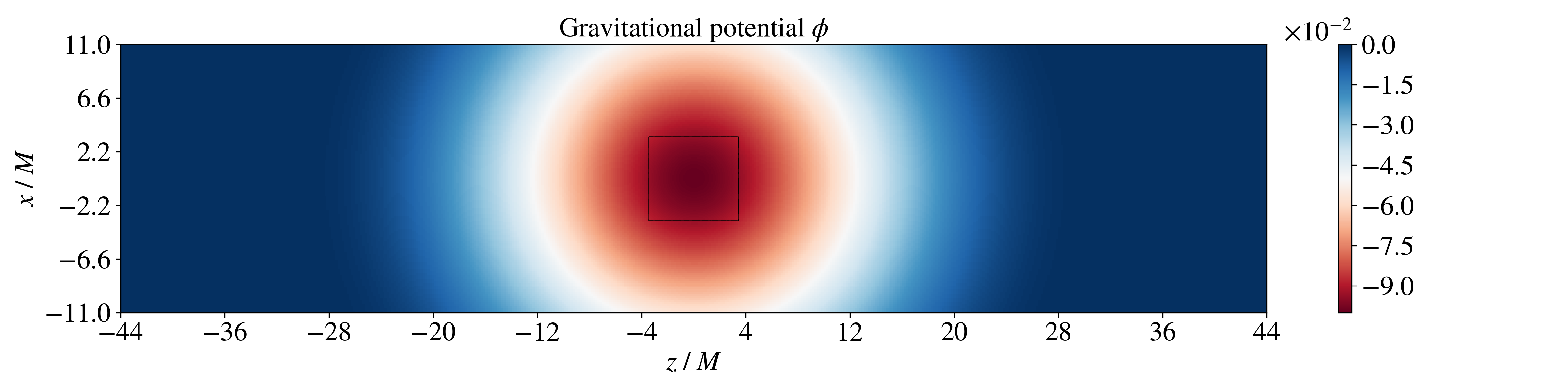
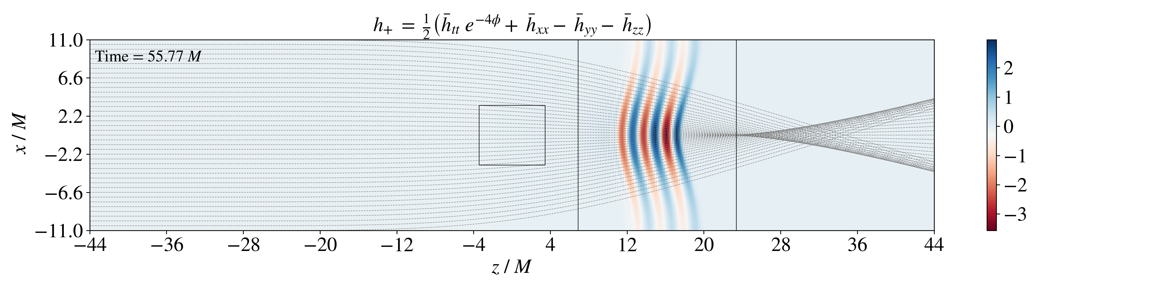
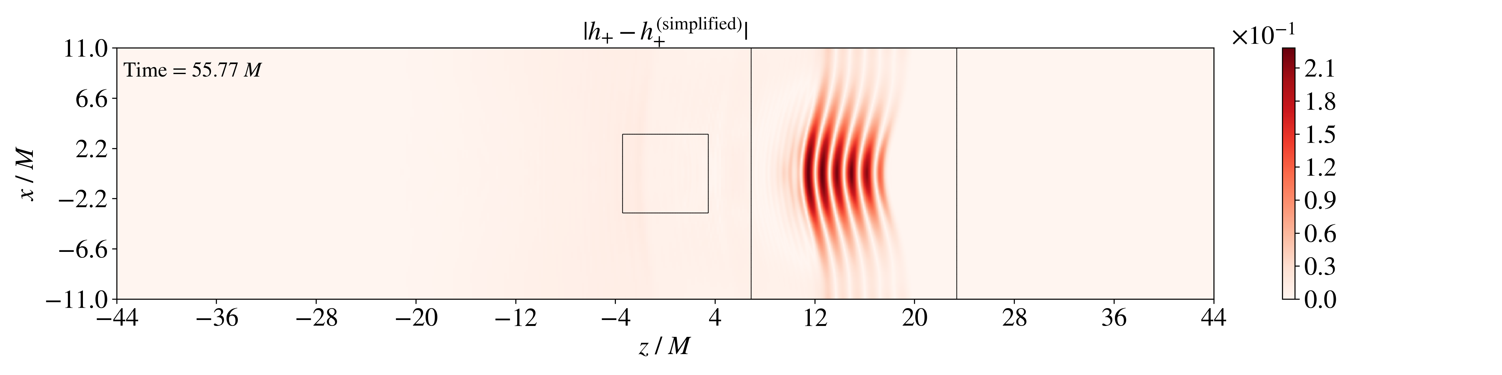
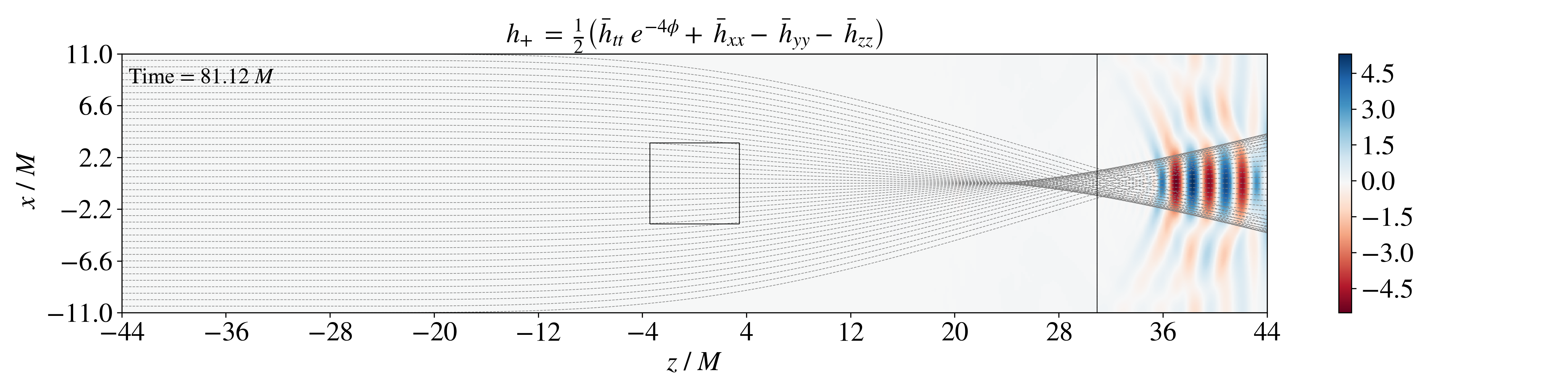
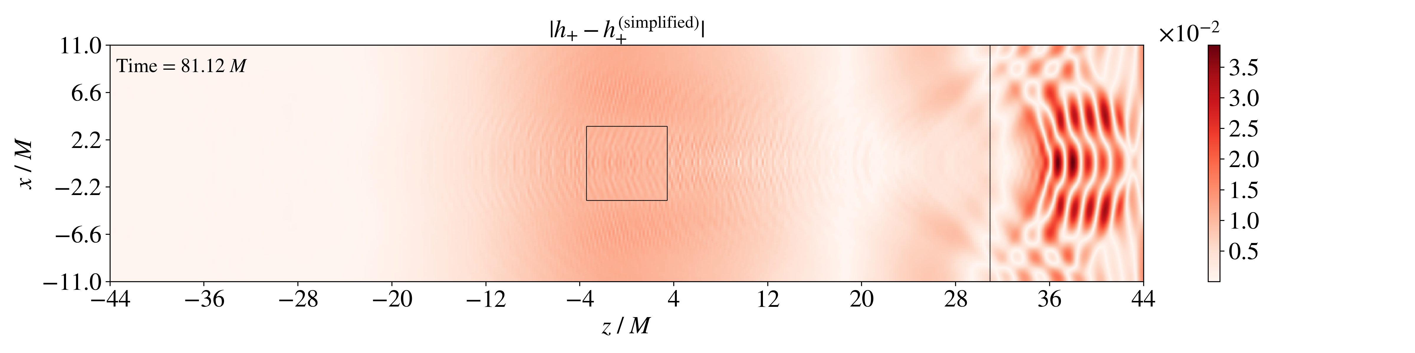
Figure 8: From top to bottom: Top figure shows the distribution of gravitational potential \(\phi\) along \(x-z\) axis for Burkert potential in weak gravity regime with \(T_{\mu \nu} = 0\). The second figure shows the 2D slice of \(h_+\) after the wave has traversed the central density at \(t=55.77 \;M\). Third figure shows the absolute difference between \(h_+\) and \(|h_+^{\text{simplified}}|\) which are evolved independently with the same initial conditions, that helps in distinguishing the effects arising from terms that are purely geometric. Fourth and fifth figure shows the wave after it had completely exited the curvature at a later time \(t=81.12 \;M\). The figure for \(h_+\) has an overlay of null geodesics for the potential configuration considered with spline. The black outlined boxes inside the simulation domain is where the AMR patch exists and has twice the resolution of base grid..
5.4 Burkert potential - strong gravity case (with \(T_{\mu \nu} =0\))↩︎
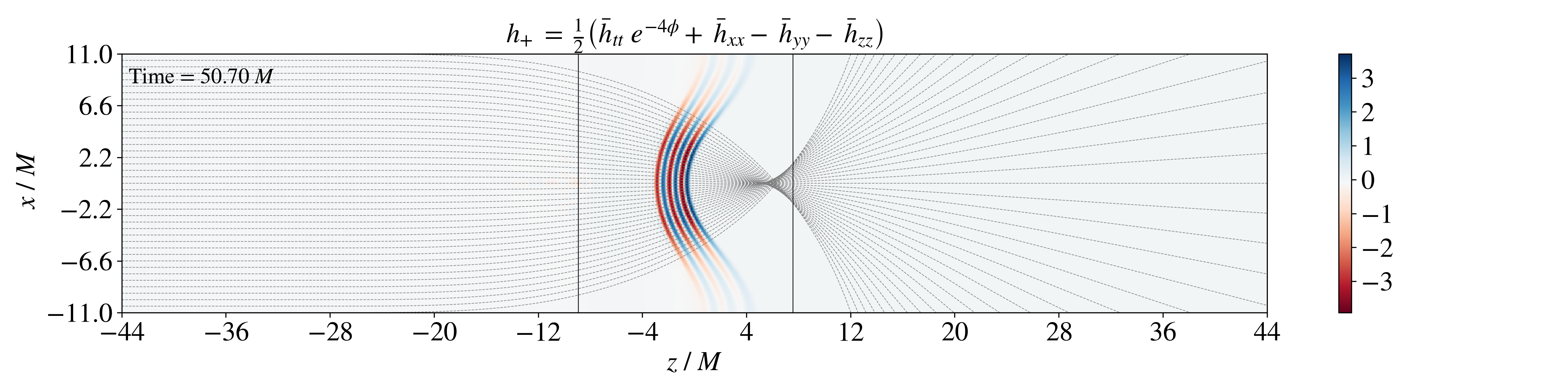
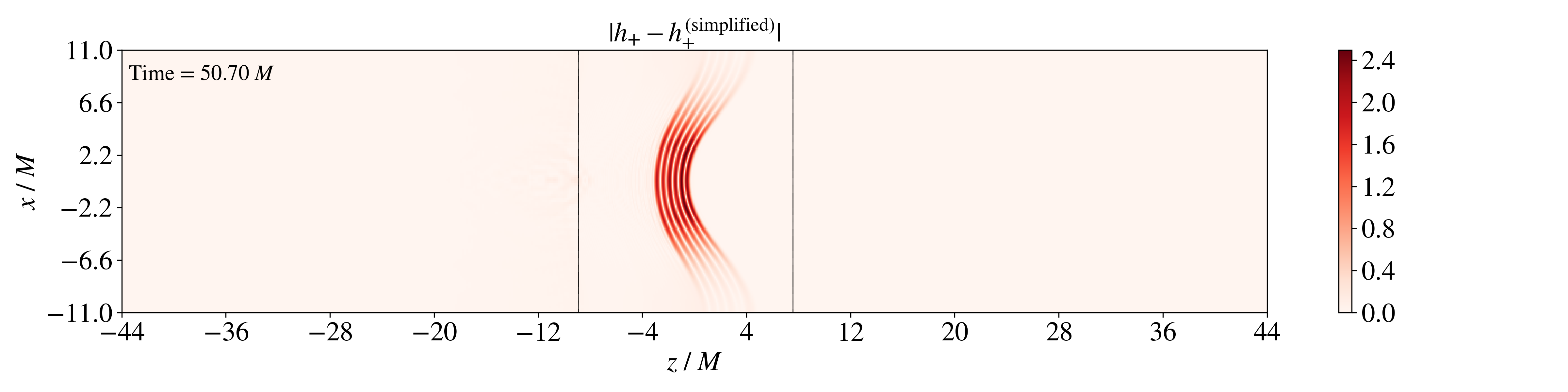
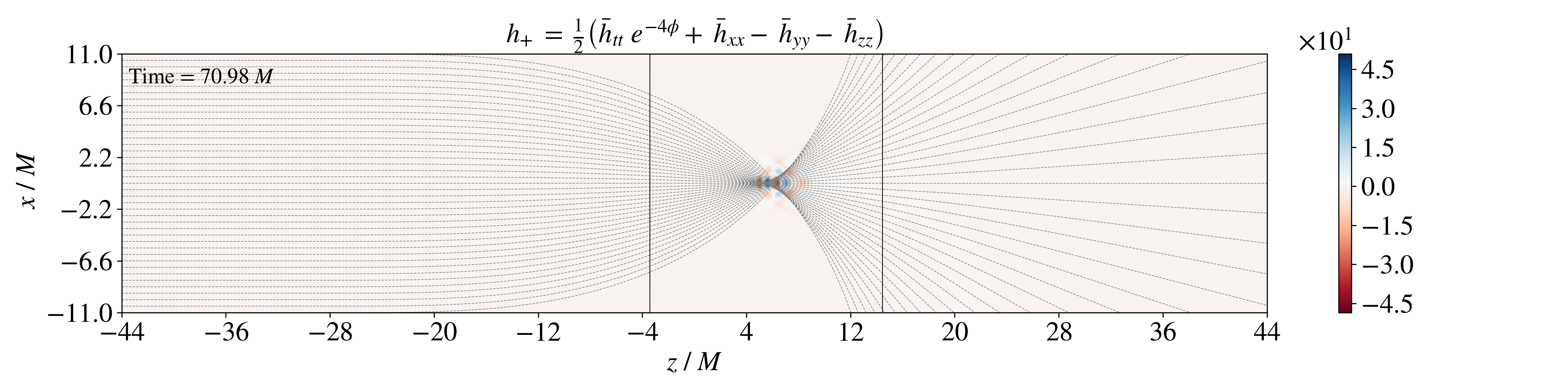
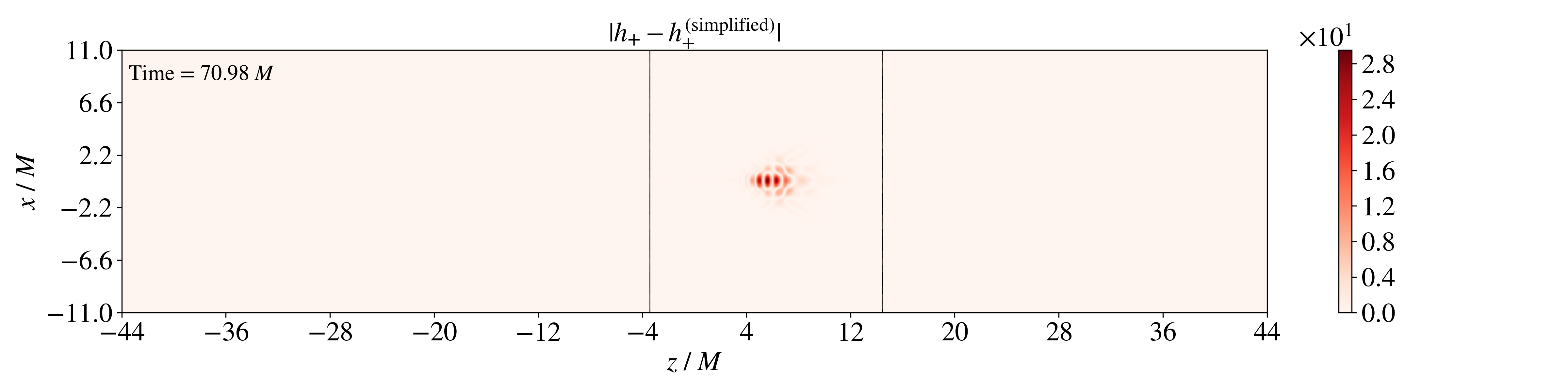


Figure 9: 2D slices of \(h_+\) for wave wave propagation through Burkert potential in strong gravity regime. From top to bottom: Top figure shows the \(h_+\) after the wave has traversed the central density at \(t=50.7 \;M\). Third figure shows the absolute difference between \(h_+\) and \(|h_+^{\text{simplified}}|\) which are evolved independently with the same initial conditions, that helps in distinguishing the effects arising from terms that are purely geometric. Fourth and fifth figure shows the wave at its maximum amplitude and the difference between \(|h_+^{\text{simplified}}|\) at that instance. The last two figure shows the wave scattering after it traversed through the peak potential and its difference at a later time \(t=91.27 \;M\). The figure for \(h_+\) has an overlay of null geodesics for the potential configuration considered with spline. The black outlined boxes inside the simulation domain is where the AMR patch exists and has twice the resolution of base grid..
In this subsection, we present the results for GW propagation through the Burkert potential in the strong gravity regime, corresponding to \(\phi_{\mathrm{max}}=-0.49\), with \(T_{\mu
\nu}=0\). Figures 9 the two-dimensional evolution of the \(h_+\) component as the wave propagates from left to right through the lens. The results are presented in terms of the
observable \(h_+\). As in the earlier simulations, the incident plane wave is initially located in a flat Minkowski region on the negative \(z\)-axis and propagates toward positive \(z\). Figure 9 shows the evolution at three representative times. The first snapshot, at \(t=50.70\,M\), corresponds to the stage when the wave is about to
enter the peak-potential region. The second, at \(t=70.98\,M\), is taken shortly after the wave has propagated through the central density. The final snapshot, at \(t=91.27\,M\), shows the
later stage of the evolution. In the two first snapshots, the difference \(|h_+ - h_+^{\text{simplified}}|\) is significantly stronger than in the earlier simulations.
In the second snapshot (\(t=70.98\,M\)) the wave exhibits strong focusing (convergence of null geodesics), and the maximum interference occurs in a localized region approximately within \(4<z<10\). This is why the amplitude is so strongly enhanced in this region. At the later time \(t=91.27\,M\), the wave is scattered over a broad angular range, extending from negative to
positive \(x\)-directions and almost resembling an approximately spherical wave source. In particular, we note that the wave front has now flipped its convexity. This did not happen in the simulations with the Gaussian and
NFW profiles. Furthermore, a small part of the wave remains within the central potential region. At this stage, the difference \(|h_+ - h_+^{\text{simplified}}|\) decreases to order \(10^{-1}\). We do not show the subsequent evolution, since reflections from the \(x\)-boundaries begin to dominate the dynamics and no longer provide physically useful information.
Figure 4 (f) shows the evolution of the maximum amplitude of the waves \(h_+\) and \(|h_+^{\text{simplified}}|\), tracked along the principal axis. The
strongest amplification occurs in the region where the null geodesics exhibit the greatest overlap, as shown in the Fig. 9 overlay, namely in the region \(0<z<4\). After the wave
has traversed this region, the amplitude decreases (corresponding to null geodesics divergence). All such wave propagation effects are in line with null geodesics predictions. Although a substantial difference develops between \(h_+\) and \(h_+^{\text{simplified}}\) while the wave passes through the central density, their final amplitudes become closer again and differ at the level of \(10^{-1}\).
6 Summary and Conclusions↩︎
We have investigated gravitational wave (GW) lensing in the wave optics regime by numerically propagating plane GW packets through spherically symmetric spacetime inhomogeneities representing e.g. dark matter halos. Such analyses are of particular
interest for future GW observations, including those by pulsar timing arrays (PTAs), since lensing-induced distortions of the waveform in the wave optics regime may provide an additional probe of the underlying matter distribution.
A central goal of this work was to go beyond the usual linearized treatment of wave propagation and instead evolve the full Einstein equations. Overall, the six resulting simulations show that the qualitative behaviour of GW propagation is controlled
jointly by the lens profile and the strength of the gravitational potential. In the weak gravity regime, all three considered density profiles (Gaussian, NFW, and Burkert) exhibit the expected signatures of Shapiro time delay and moderate focusing, with
the locations of maximum amplification broadly consistent with the corresponding null geodesic convergence regions. In this regime, the simplified evolution equation reproduces the main features of the full solution reasonably well, and the final
discrepancies remain small, only of a few percent.
The situation changes significantly in the strong gravity regime. There, the wave dynamics become more sensitive to the full geometric structure of the spacetime, and the propagation can no longer be described adequately by the simplified evolution alone.
In particular, we find that the wave may develop pronounced tails, multidirectional scattering, and stronger deviations from the null geodesic expectation when it traverses the central high curvature region. The comparison between the full Einstein
equation evolution and the corresponding vacuum evolution indicates that the presence of the density source induces corrections at the level of a few percent in the propagated GW signal. This is consistent with recent analytical work [70] that finite-wavelength propagation through matter distributions can lead to deviations from the pure geometric-optics limit. For sufficiently precise GW
observations, such effects may therefore become relevant for accurate signal modelling and could, in principle, provide additional information about the dark-matter environment.
Our simulations also show that the structure and shape of the gravitational potential plays an important role in determining the lensing phenomenology. The amplification is not controlled solely by the total mass of the lens, but also by the shape of the
potential and, more specifically, by how sharply it focuses the null-ray bundles. This is evident from the comparison among the Gaussian, NFW, and Burkert profiles. In particular, the strong gravity Burkert case exhibits the most pronounced amplification,
with the peak amplitude increasing by nearly a factor of \(30\) relative to the incident wave. More generally, while the full and simplified evolutions can differ substantially when the wave is inside the central curvature
region, the discrepancy typically decreases after the wave exits the lens, often settling to the level of a few percent. This suggests that the curvature dependent terms in the full Einstein equations have their strongest impact while the wave is
traversing the high curvature region, rather than producing a large cumulative effect far from the lens similar to Integrated Sachs-Wolfe effect [71]
.
A further conclusion of this work is that the simplified evolution equation is reliable only in restricted regimes. In the weak gravity simulations, it reproduces the main features of the full solution reasonably well, at least qualitatively and often
semi-quantitatively. In the strong gravity cases, however, its limitations become evident. In particular, it does not capture the full multidirectional scattering pattern that appears when the wave interacts with the central density, nor does it fully
reproduce the large transient amplification observed in the strongest focusing configurations. Furthermore, for the Burkert profile in the strong gravity regime, the discrepancy remains large even after the wave has exited the high-curvature region: the
simplified evolution differs from the full Einstein equation result by more than \(35\%\). The simplified description should therefore be used with caution in regimes where the curvature is strong and the wavelength is not
negligible compared with the characteristic lensing scale.
It is important to note that, for the NFW and Burkert backgrounds, we have set \(T_{\mu\nu}=0\) and treated the GW evolution as propagation in a prescribed vacuum geometry. It cannot capture the full wave optics effects
that arise specifically from the coupling between the GW and the density distribution through the full Einstein equations. Although this is not a fully self-consistent matter-coupled calculation, it nevertheless provides a useful reference for isolating
the role of the background curvature and for comparing the full wave evolution with the null geodesic picture. We do believe that the presented results are valuable as the density-free results and the results including the non-vanishing density are
qualitatively similar for the Gaussian profile, where we could test the approximation. One important caveat is that once the density source is included, a weak but non-negligible component of the GW is scattered into multiple directions, with an amplitude
reaching a few percent of the overall signal in the strong gravity case. This behaviour is qualitatively similar to that seen in the weak gravity case, although its magnitude is larger here. Such multidirectional scattering is not predicted by the null
geodesic description, which only tracks the propagation of rays in the geometric-optics limit and therefore cannot account for finite-wavelength effects of this kind. The comparison therefore indicates that, when the wave propagates through a density
distribution, the full dynamics can deviate from the null geodesic approximation at the level of a few percent. Although small, this deviation is systematic and may become relevant in precision modelling of lensed GW signals. A natural extension of the
present work would therefore be to incorporate the corresponding matter distributions self-consistently, for example through numerical schemes that allow stable treatment of the central region, possibly using excision or related techniques.
From an observational perspective, our results suggest that lensing by intermediate structures may imprint subtle but potentially measurable signatures on GW signals. Such effects could otherwise be misidentified as evidence for modified gravity or other
beyond General Relativity phenomena if they are not modelled carefully. More broadly, the present analysis demonstrates that full wave simulations in curved backgrounds can provide a useful framework for disentangling propagation effects from source
physics and from genuine departures from general relativity.
Finally, several directions remain open for future investigation. In the present work, we have focused primarily on the \(h_+\) component and have not studied in detail the behaviour of the other components of \(h_{\mu\nu}\) during propagation through curved spacetime. It would be particularly interesting to investigate polarization mixing and possible birefringence-like effects in more general settings. Additional extensions include
self-consistent matter-coupled simulations for NFW and Burkert profiles, improved numerical infrastructure with AMR and better absorbing boundaries, and a more systematic analysis of how the lens profile, wave frequency, and source-lens-observer geometry
jointly determine the observable waveform distortions.
In summary, our results show that GW propagation in curved spacetimes is well approximated by the geometric optics picture only in sufficiently weak gravitational fields. In stronger curvature regimes, finite-wavelength effects, density induced
corrections, and the detailed structure of the lens can produce non-trivial modifications of the waveform that are not captured by simplified evolution equations alone. Accurate modelling of such phenomena therefore requires the full Einstein equations and
will be increasingly important as GW observations enter a regime of greater precision and sensitivity. In addition, when training machine learning models to make inferences based on GW data including lensing data, there is a risk of obtaining biased
results if the training is done on simple, analytical models (as in e.g. [72]) instead of more realistic simulations (see e.g. [73] for some of the many considerations necessary for good machine learning training).
This project is funded by VILLUM FONDEN, grant VIL53032 (PI: SMK). Research at Perimeter is supported by the Government of Canada through the Department of Innovation, Science, and Economic Development, and by the Province of Ontario through the
Ministry of Colleges and Universities. Part of the computational work was performed using Perimeter’s HPC system”Symmetry".
APS thanks Mandana Amiri and Mark Halpern of the Physics and Astronomy department, University of British Colombia (UBC) for hosting him during his research stay at UBC where part of this work was carried out.
Author contribution statement: APS performed the analytical computations. APS performed the numerical work under the guidance of SMK, RH and ES. Analysis of the numerical work was led by APS but all authors contributed. Conclusions were
drawn by APS and SMK who jointly wrote the manuscript with comments from ES and RH.
7 Null geodesics↩︎
In this appendix we review the geodesic equations for our background spacetime and explain how these were solved to obtain the geodesic overlays presented in the figures in the main text. Further, in figure 10 we plot
null geodesics for the spacetimes with versus without the spline approximation to demonstrate that the introduction of the spline and corresponding negative density only has minimal impact on the results.
The geodesic equations corresponding to the line element in equation 1 are \[\frac{d^2 t}{d\lambda^2}
+ 2 \frac{dt}{d\lambda}
\left(
\phi_x \frac{dx}{d\lambda}
+ \phi_y \frac{dy}{d\lambda}
+ \phi_z \frac{dz}{d\lambda}
\right)
= 0,\] \[\frac{d^2 x}{d\lambda^2}
=
\phi_x \left(
e^{4\phi} \left(\frac{dt}{d\lambda}\right)^2
- \left(\frac{dx}{d\lambda}\right)^2
- \left(\frac{dy}{d\lambda}\right)^2
- \left(\frac{dz}{d\lambda}\right)^2
\right),\] where \(\lambda\) is an affine parameter along the ray. When solving these equations for our spacetime setups, we assume that both the initial positions and tangent vectors lie in the equatorial plane. For
an incident plane wave, the corresponding ray bundles are therefore initially parallel to one another along the \(x\)-axis. These correspond to wavefronts propagating from left to right across the simulation domain. Figure
10 shows six representative configurations for the Gaussian, NFW, and Burkert cases in both the weak and strong gravity regimes. In each plot in fig. 10, the black dot marks the centre of
the lens/density distribution. In these figures we show lines of null geodesics for the gravitational potential with and without the spline approximation plotted on top of each other. We see that the deviation of null geodesic due to the spline is similar
and only affects the focusing distance of the GWs for Gaussian and NFW potential in both weak and strong gravity. For Burkert potential, the spline affects focusing distance and as well as how tightly the rays are focused. Despite these differences,
qualitatively the behaviour of spline vs. no-spline geodesics are similar.
Since the propagation direction is given by the normal to the wavefront, the null geodesics provide a useful geometric characterization of the GW trajectories. Although we do not explicitly construct the normals to the simulated wavefronts, we compare the
geodesics with the observed propagation direction of the waves on a visual basis to assess whether the rays are roughly orthogonal to the wave fronts.
The plots in figure 10 show that the different potential configurations considered produce qualitatively different focusing behaviour. In the weak gravity regime, the rays are only moderately deflected and converge at a
finite focal point determined by the lens profile. In the strong gravity regime, however, the deflection near the lens is much stronger and the rays no longer form a finite focal point of the type seen in the weak gravity case. Instead, the ray structure
becomes more distorted in the vicinity of the central potential.
The crossings of neighbouring ray bundles seen in the plots indicate the regions where the gravitational waves are expected to interfere constructively and hence produce enhanced intensity. Thus, the null geodesics provide a useful geometric guide for
interpreting the main features observed in the full wave simulations.
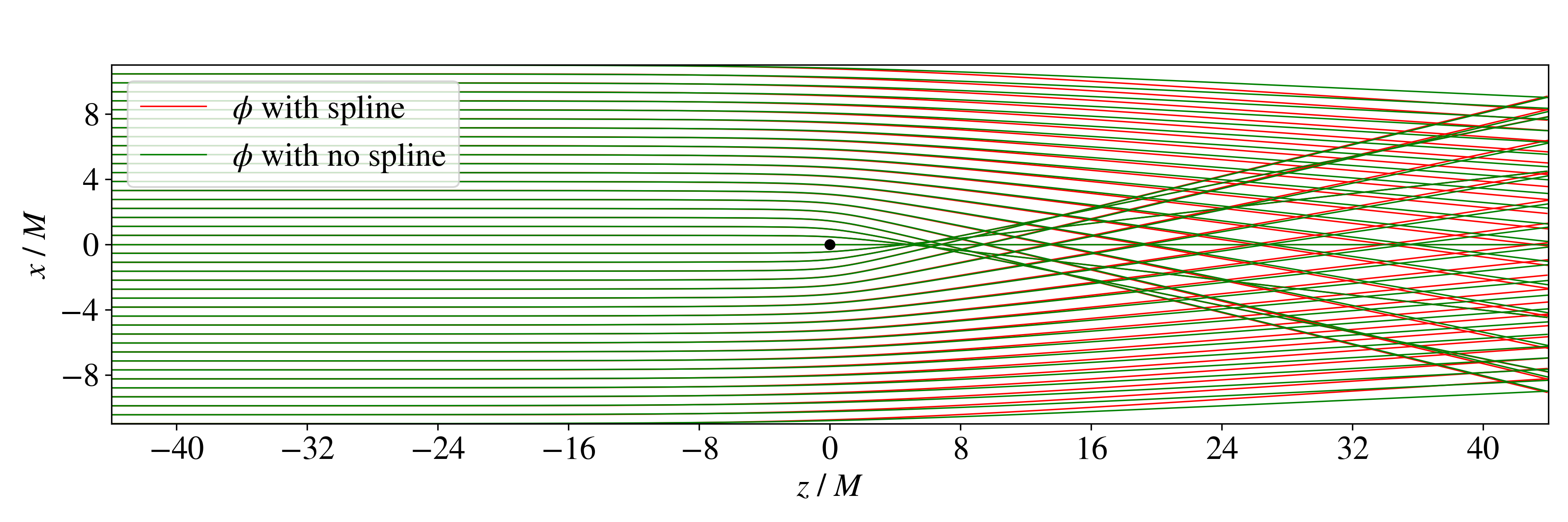
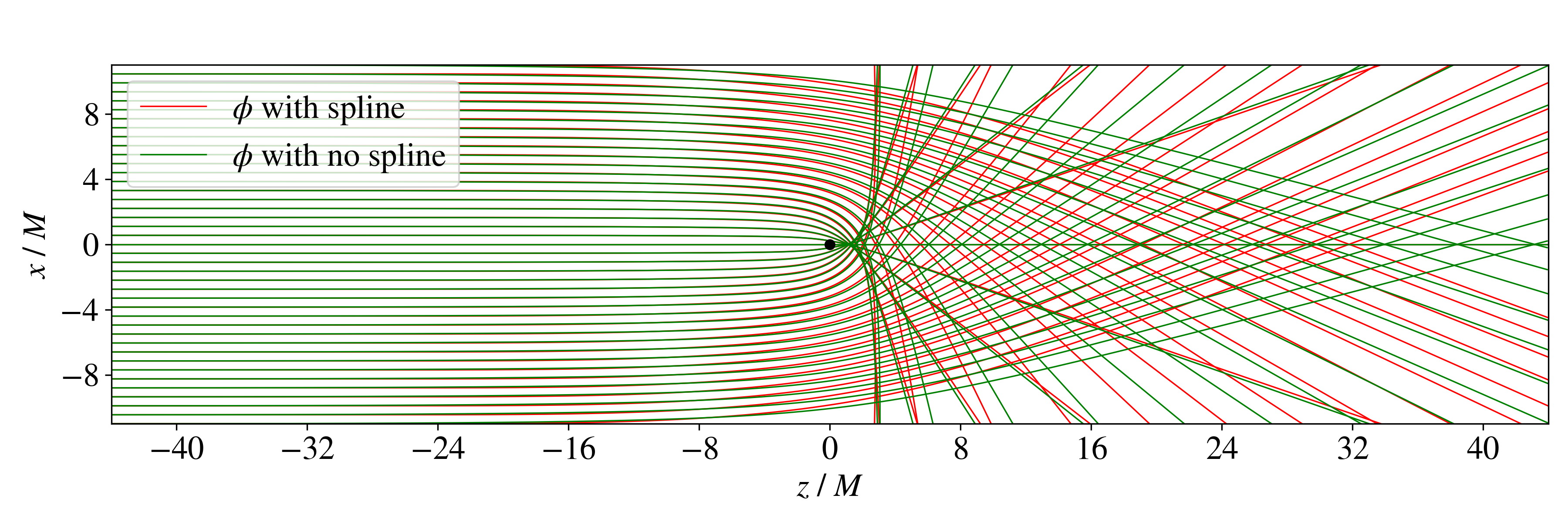
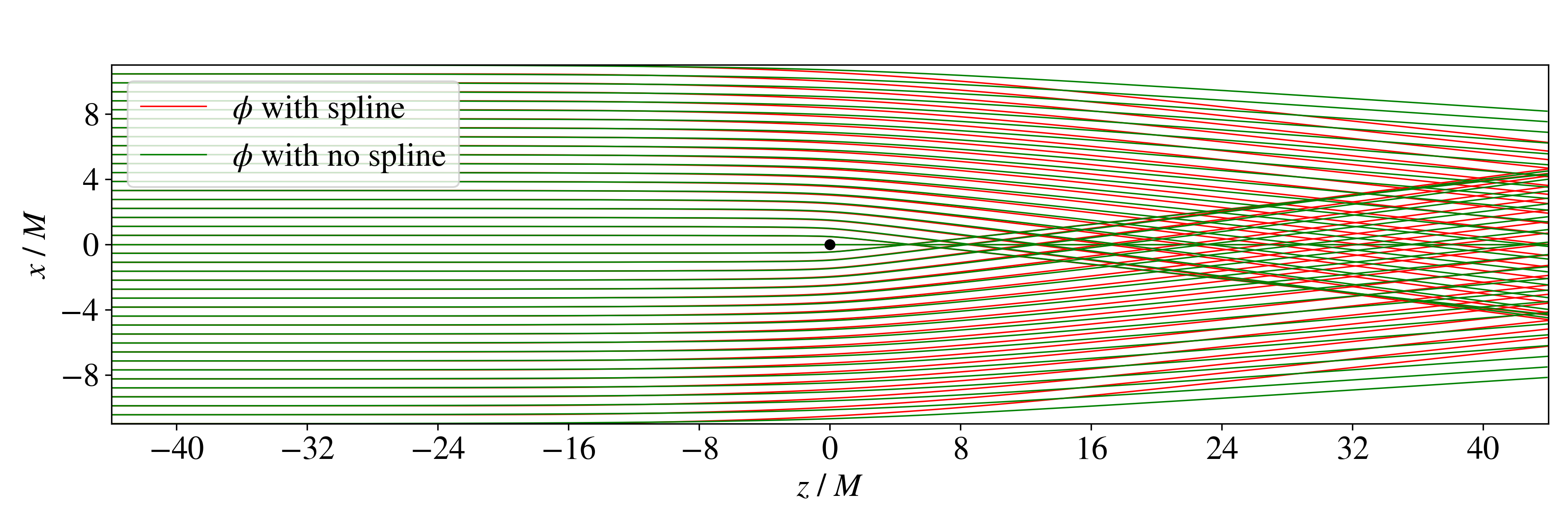
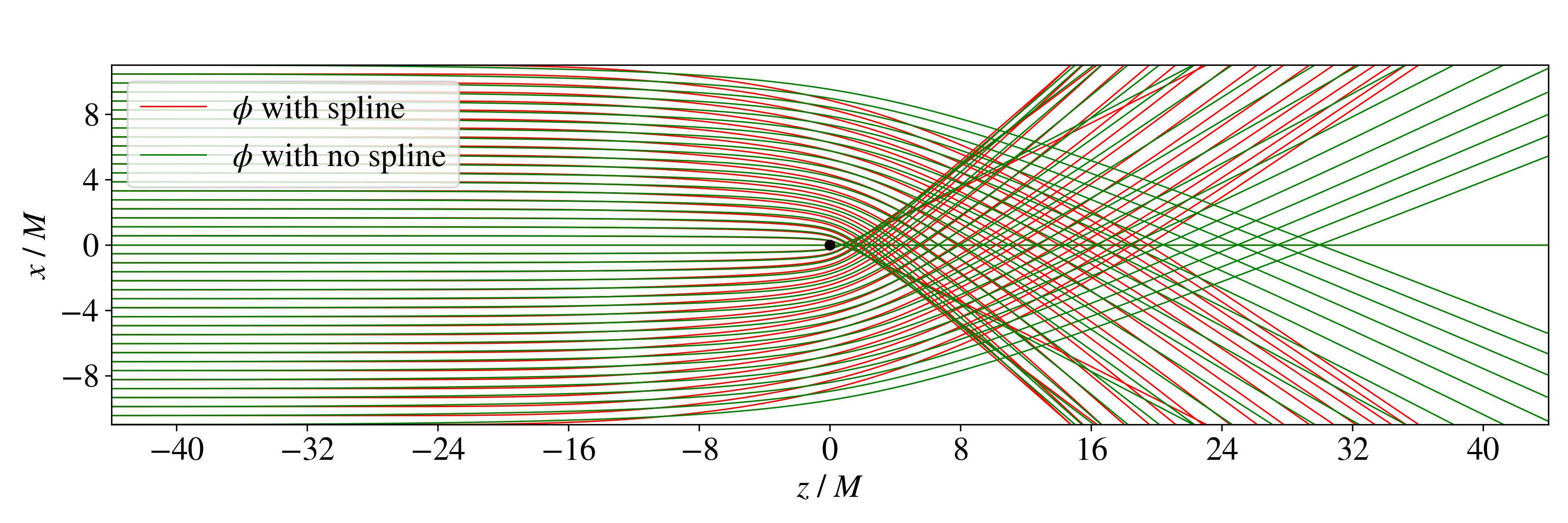
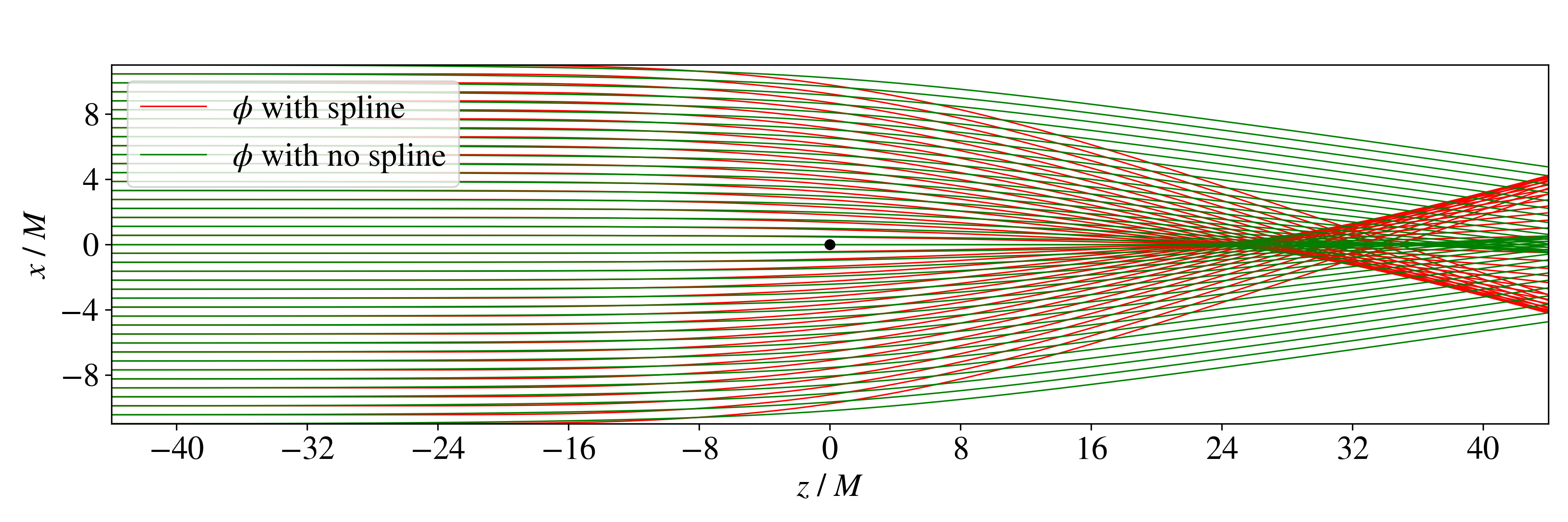
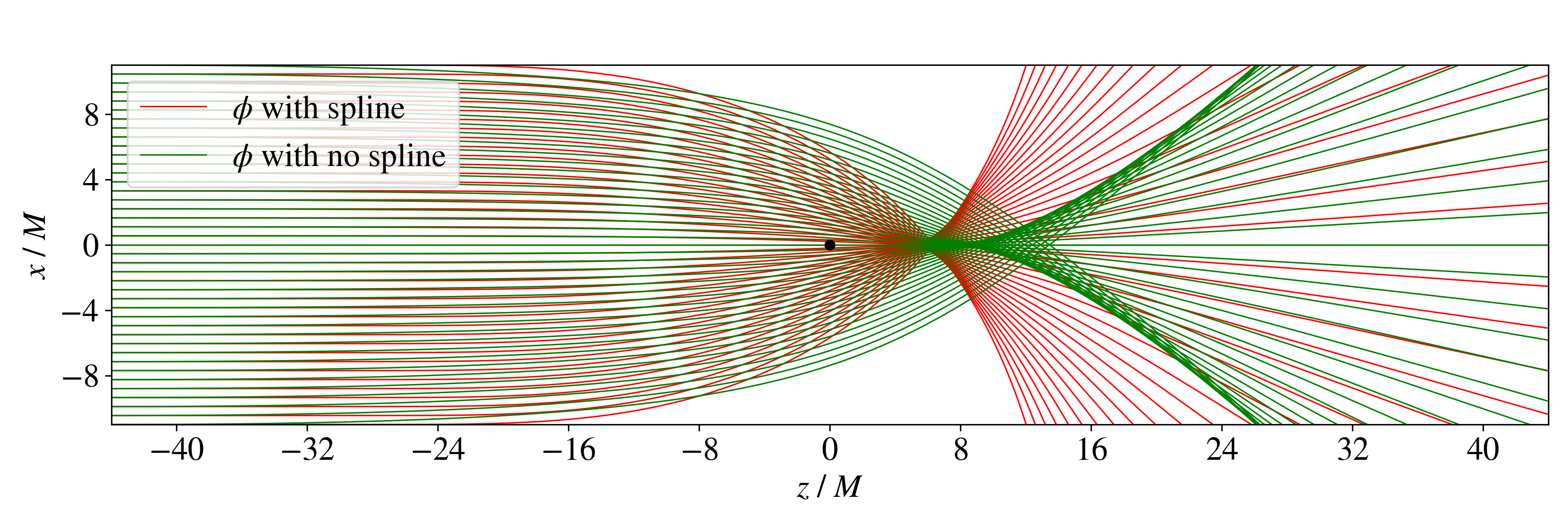
Figure 10: null geodesic trajectories of a plane wavefront for three gravitational potentials for the Gaussian, NFW, and Burkert profiles with \(\phi_{\text{max}} = -0.1\) and \(\phi_{\text{max}} = -0.49\) corresponding to the weak and strong gravity case. The black dot denotes the peak curvature point. Here we show that the deviation of null geodesic due to the spline is similar and only affects the focusing distance of the GWs.. a — Null geodesics for Gaussian potential - weak gravity case, b — Null geodesics for Gaussian potential - strong gravity case, c — Null geodesics for NFW potential - weak gravity case, d — Null geodesics for NFW potential - strong gravity case, e — Null geodesics for Burkert potential - weak gravity case, f — Null geodesics for Burkert potential - strong gravity case
| Spline distance from \(\phi_{\text{max}}\) | \(r_1\) | \(r_2\) |
|---|---|---|
| Gaussian potential | \(6.27 \;M\) | \(31.33 \;M\) |
| NFW Potential | \(6.27 \;M\) | \(31.33 \;M\) |
| Burkert Potential | \(0.3133 \;M\) | \(31.33 \;M\) |
8 Numerical convergence of constraints↩︎


Figure 11: Convergence plots for the constraints \(\mathcal{C}_x\) and \(\mathcal{C}_y\) at time \(t=0.879\) for three different resolutions denoted by \(h\), \(h/2\) and \(h/4\) respectively. The data was sampled along a line from \((0,0,0)\) to \((0,0,10)\). For fourth order convergence, we expect the high resolution error to be \(16\) times lower than the low resolution error; hence, we multiply the high resolution error by a factor of \(2^4\) to show numerical convergence..
To show that the numerical simulations presented in this work are valid and preserve the Lorenz gauge, we here present a convergence test using the constraint violation to demonstrate that the constraints converge. We perform three simulations (with no
AMR) with grid resolutions \(128 \times 128 \times 512\), \(256 \times 256 \times 1024\) and \(512 \times 512 \times 2048\) denoted by \(h\), \(h/2\) and \(h/4\) respectively. We set the domains for \(\{x,y,z\}\) as \(\{(-4<x<4),(-4<y<4),(-10<z<10)\}\). We initialize plane wave \(\bar h_{+}\) and \(\bar h_{\times}\) as
\[\label{lokciuys} \begin{align} \bar h_+ & = \cos[ 2 \pi (k_zz-\omega t)] \\ \bar h_\times & = \sin[ 2 \pi (k_zz-\omega t)], \\ \end{align}\tag{8}\] with \(k_z \simeq 1.47\) in a Gaussian background (with weak gravity setting \(\phi_{\text{max}} = -0.1\)). The wave is
initialized with the same non-vanishing amplitude over the entire domain, ensuring an initial constrain violation. Although, it is unphysical (and does not satisfy Lorenz gauge) to initialize plane waves as in eqn. [eq:planewave95conv] in curved spacetime, we choose these initial conditions in order to demonstrate that the constrain damping method efficiently suppresses constraint violations.
We set \(\partial_t \bar h\) such that the wave propagates along the z-axis. We use reflecting boundary conditions in all three spatial dimensions and use constraint damping as specified in section 3.4.
We compute the absolute difference between constraint violation \(\mathcal{C}\) defined by eqn. 5 , i.e. we calculate \(\left| \mathcal{C}_v ^{ h} - \mathcal{C}_v ^{ h/2}
\right|\) and \(\left| \mathcal{C}_v ^{ h/2} - \mathcal{C}_v ^{ h/4} \right|\) at three time instances. We verify the order of convergence, \(p\), which should be \(p=4\) in our case. Therefore,
\[\label{conv95eqn} \begin{align} \left| \frac{\mathcal{C}_v ^{ h} - \mathcal{C}_v ^{ h/2}}{\mathcal{C}_v ^{ h/2} - \mathcal{C}_v ^{ h/4}} \right| &= 2^p + O(h).\\ \text{or, } |\mathcal{C}_v ^{ h} - \mathcal{C}_v ^{ h/2}| & \simeq 2^4 |\mathcal{C}_v ^{ h/2} - \mathcal{C}_v ^{ h/4}| . \end{align}\tag{9}\]
Figure 11 compares the errors of the simulations with the three different resolutions. The errors seen in the subfigures agree with eqn. 9 , demonstrating that the constraints converge. The subfigures also demonstrate that with increasing simulation resolution, the constraint violation tends toward zero. This shows that the constraint violations developed during the evolution are due to the numerical discretisation error and not physical constraint violation, and are efficiently damped by the constraint damping scheme.
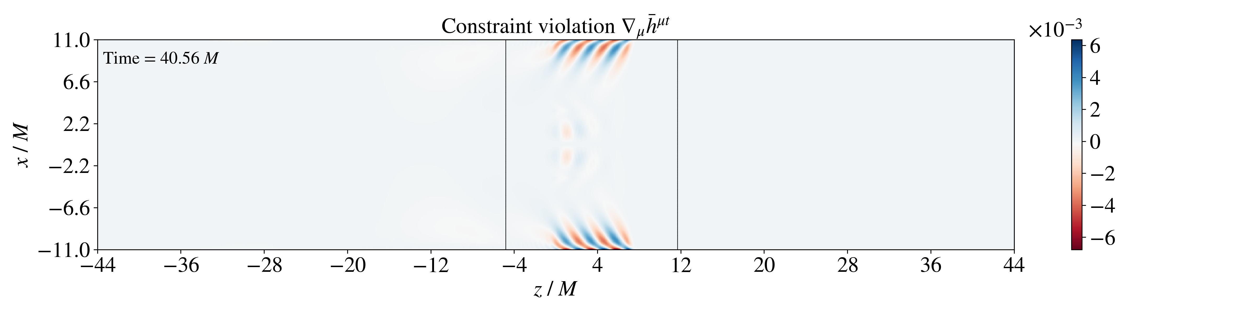
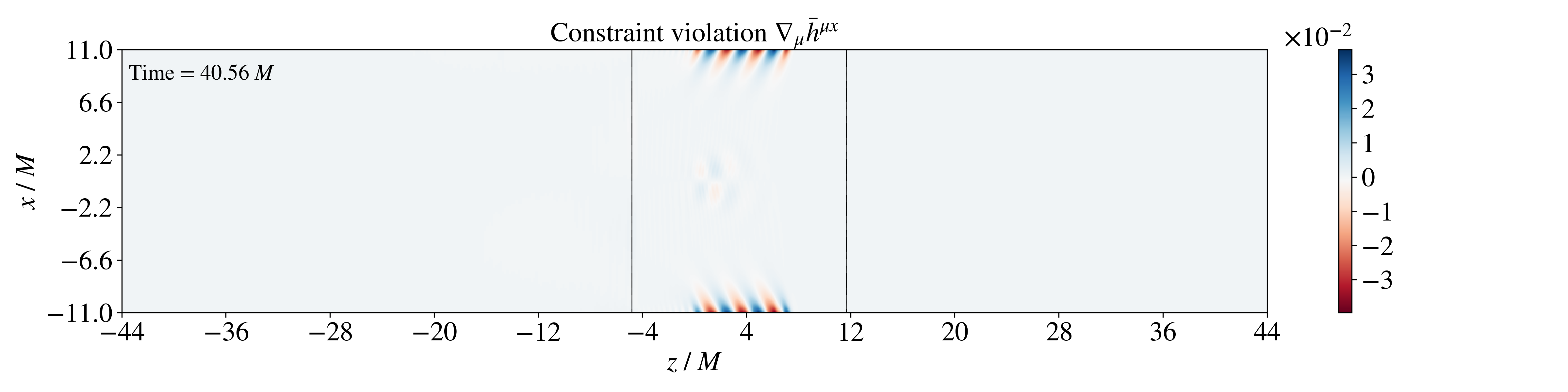
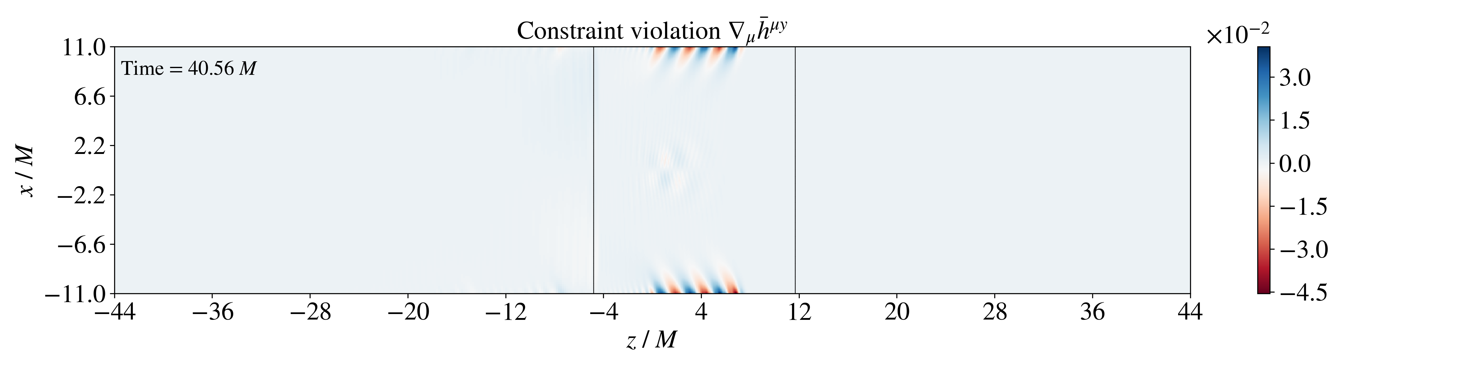
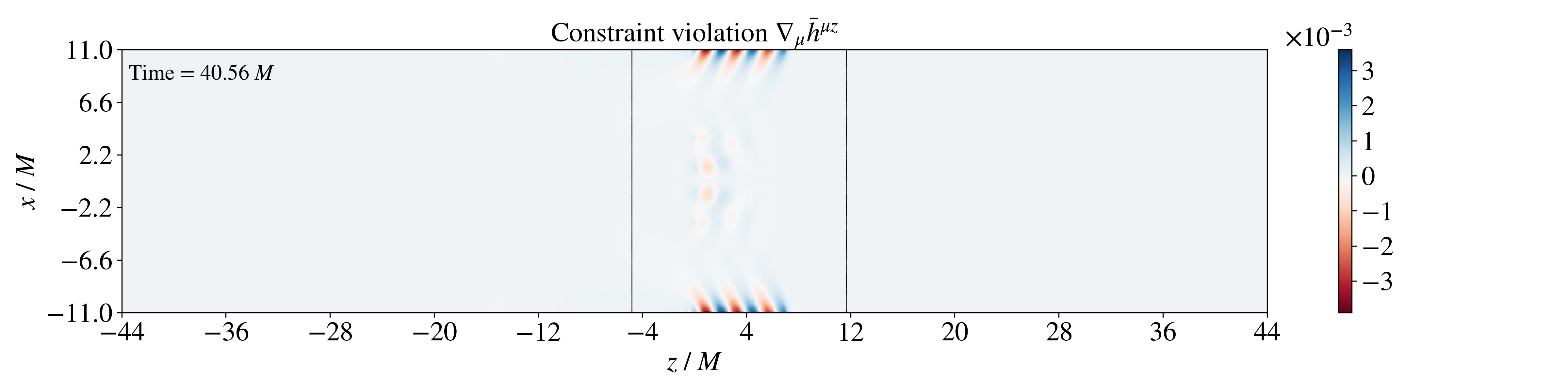
Figure 12: 2D slice of constraint violation plots at the instance when the GW is propagating inside the the Gaussian density(weak lensing case with \(\phi_{\text{max}}=0.1\)). We note that at this simulation resolution considered, the constraint violation is well below the order of GW amplitude. The black outlined boxes inside the simulation domain is where the AMR patch exists and has twice the resolution of base grid.. a — Lorenz gauge violation \(C_t\), b — Lorenz gauge violation \(C_x\), c — Lorenz gauge violation \(C_y\), d — Lorenz gauge violation \(C_z\)
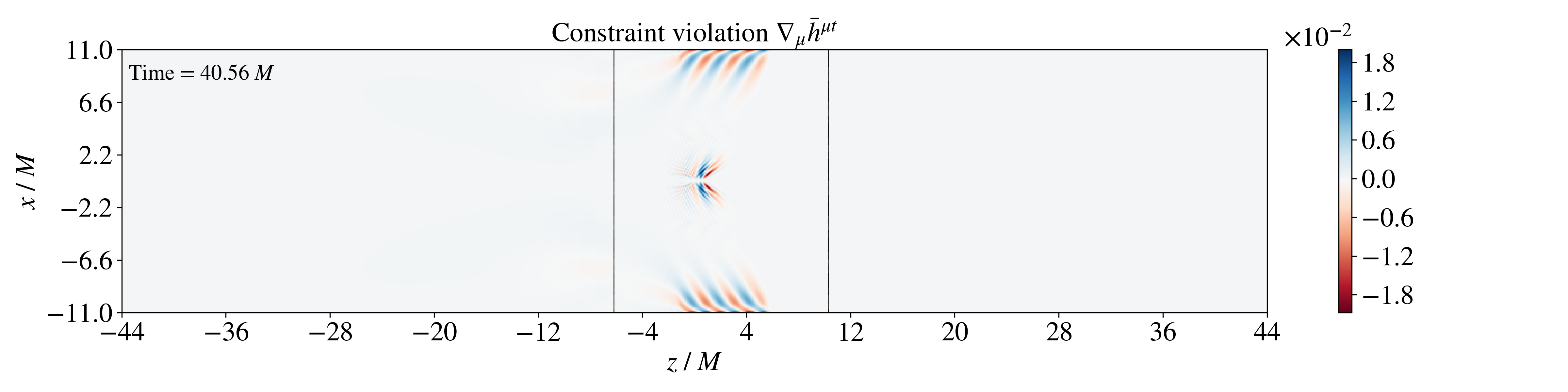
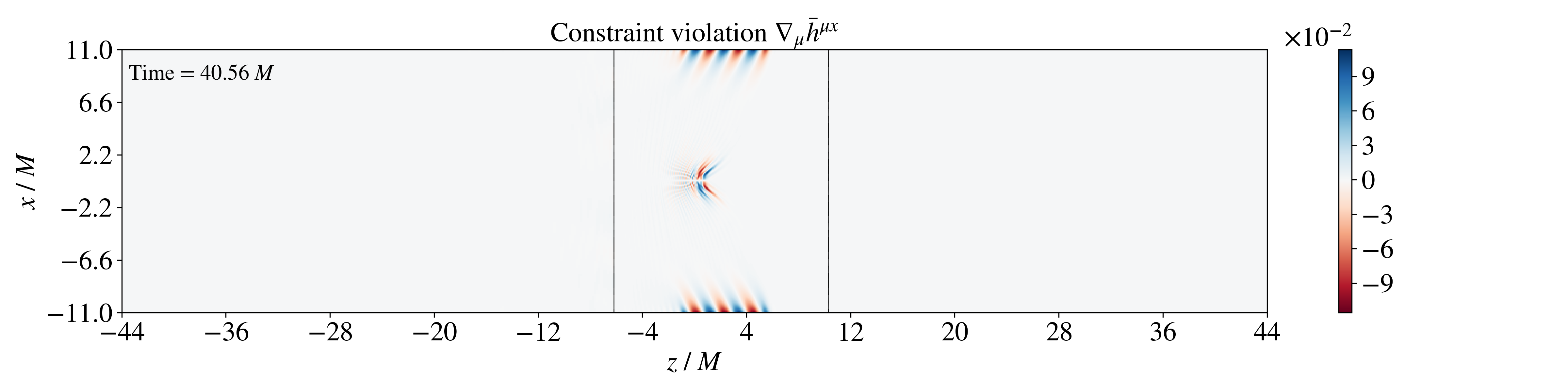
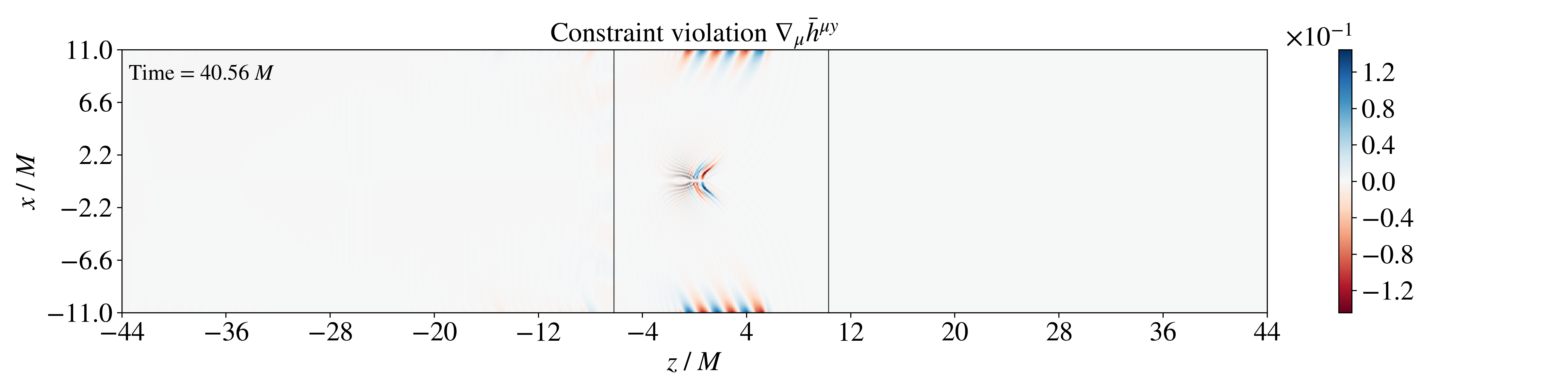
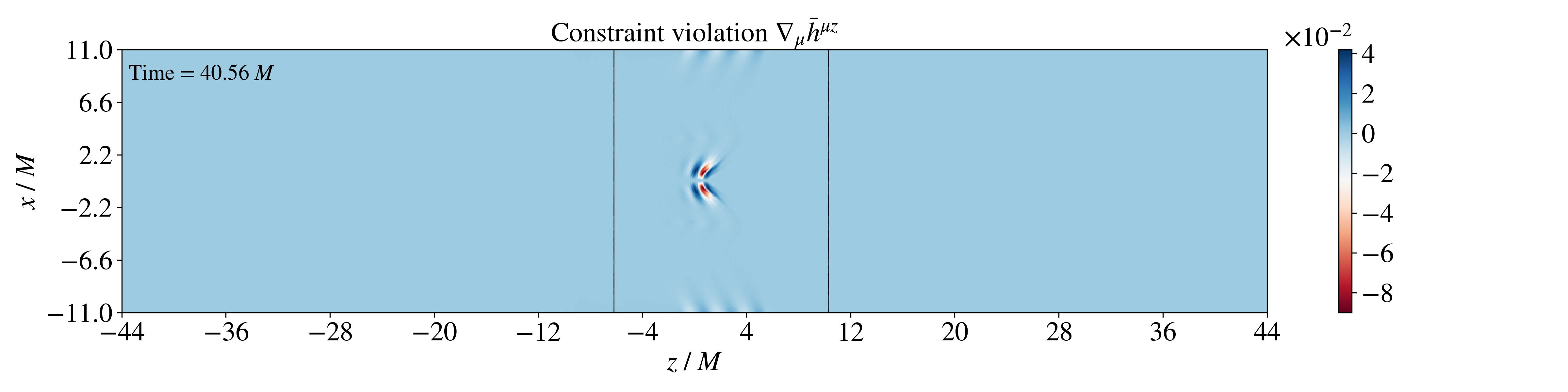
Figure 13: 2D slice of constraint violation plots at the instance when the GW is propagating inside the the Gaussian density(strong lensing case with \(\phi_{\text{max}}=0.49\)). We note that at this simulation resolution considered, the constraint violation is well below the order of GW amplitude. The black outlined boxes inside the simulation domain is where the AMR patch exists and has twice the resolution of base grid.. a — Lorenz gauge violation \(C_t\), b — Lorenz gauge violation \(C_x\), c — Lorenz gauge violation \(C_y\), d — Lorenz gauge violation \(C_z\)
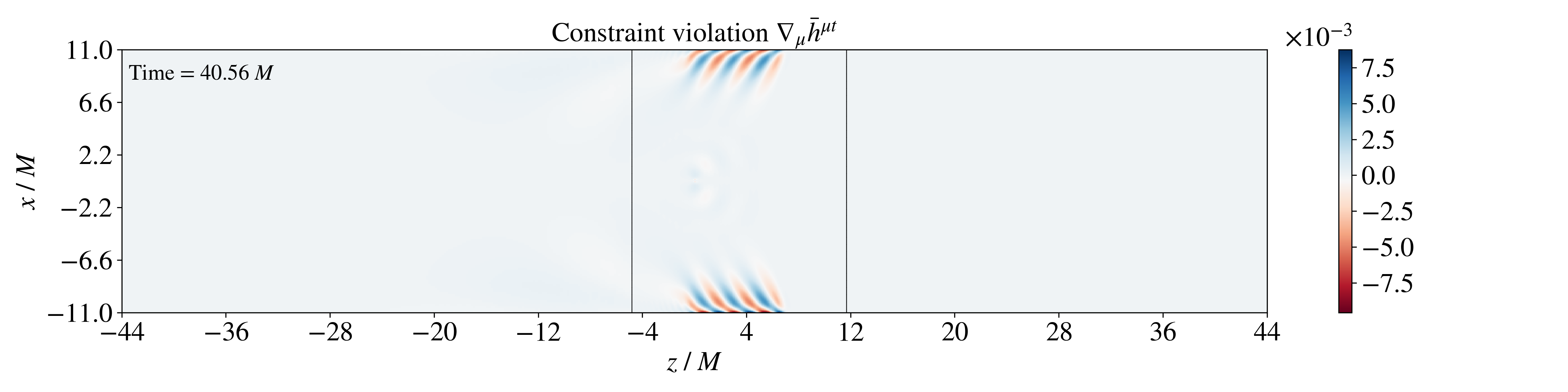
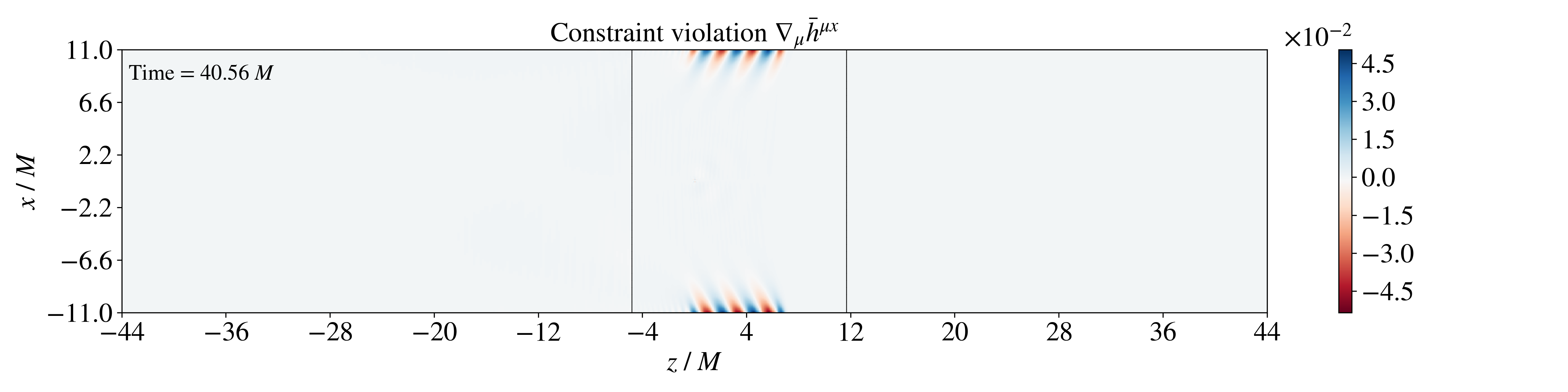
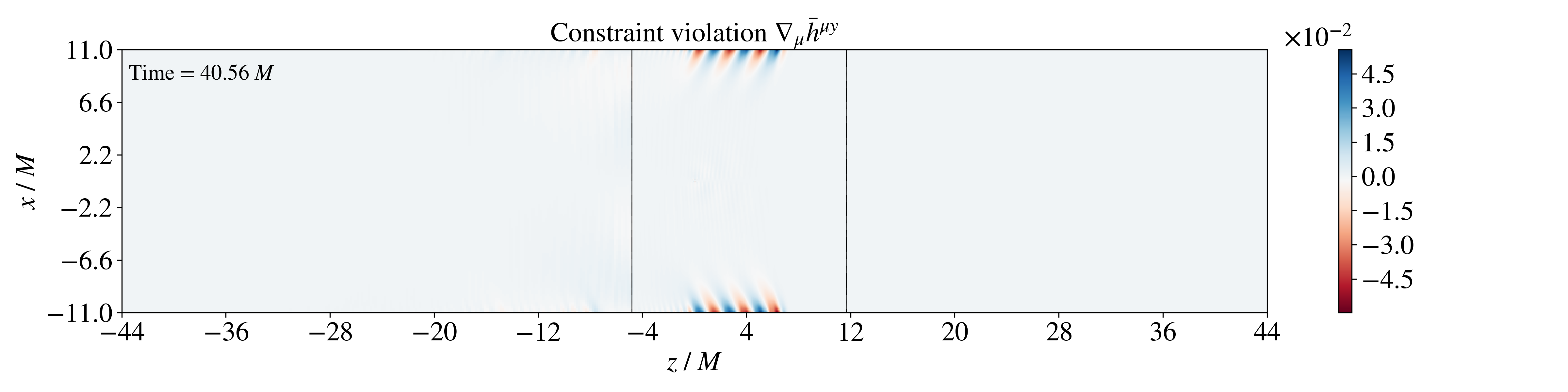
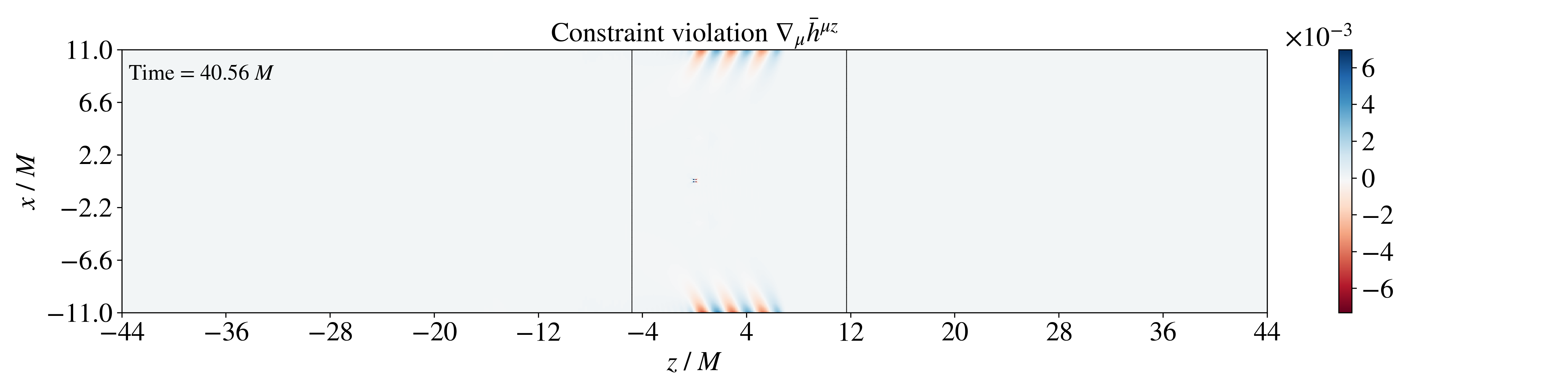
Figure 14: 2D slice of constraint violation plots at the instance when the GW is propagating inside the the NFW potential(weak lensing case with \(\phi_{\text{max}}=0.1\)). We note that at this simulation resolution considered, the constraint violation is well below the order of GW amplitude. The black outlined boxes inside the simulation domain is where the AMR patch exists and has twice the resolution of base grid.. a — Lorenz gauge violation \(C_t\), b — Lorenz gauge violation \(C_x\), c — Lorenz gauge violation \(C_y\), d — Lorenz gauge violation \(C_z\)
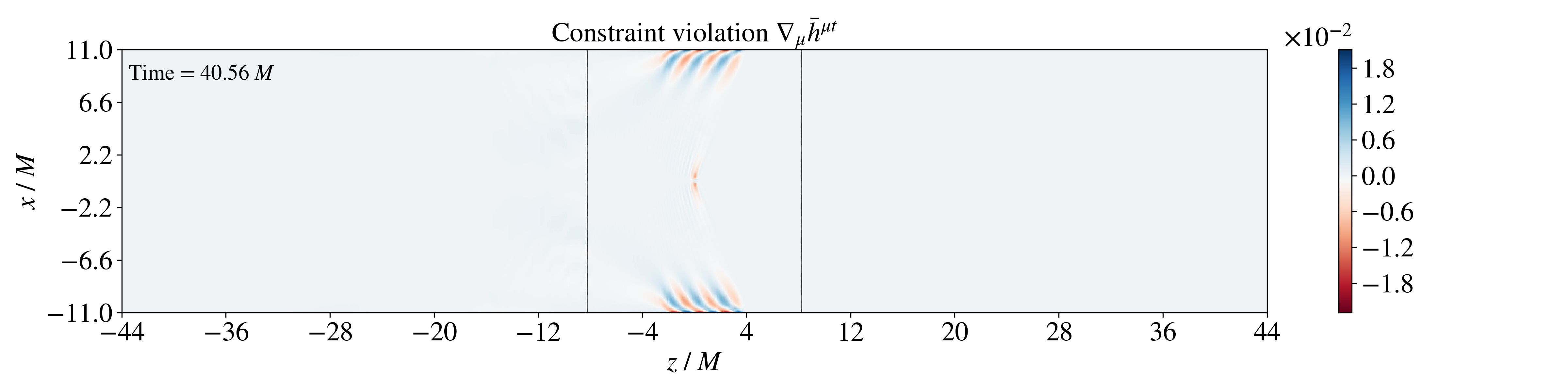
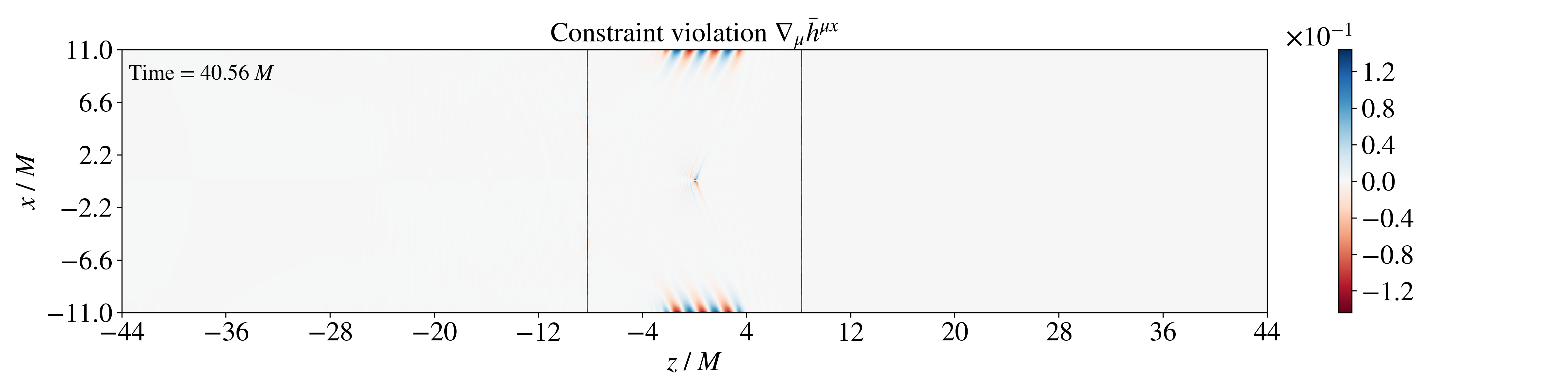
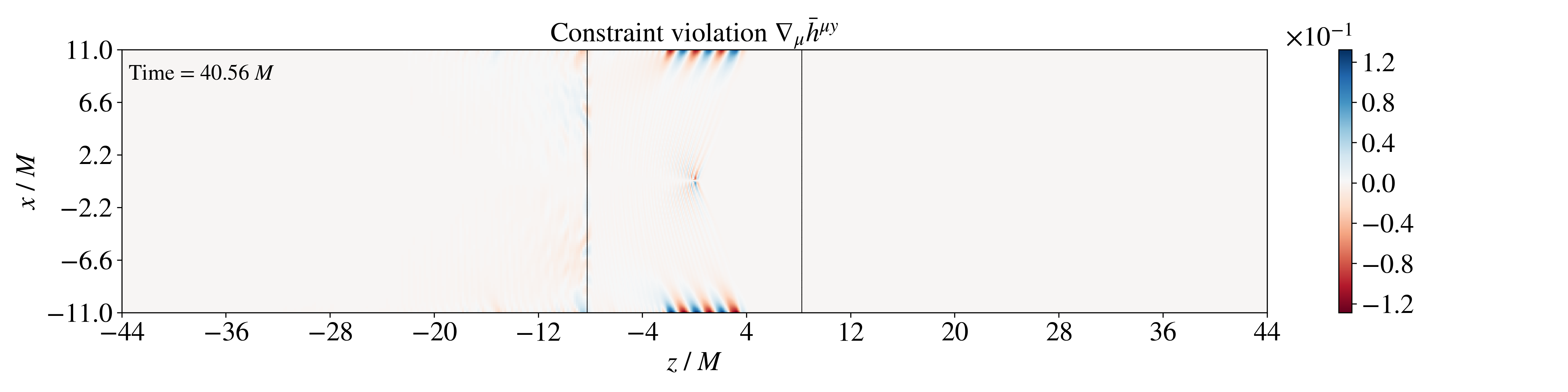
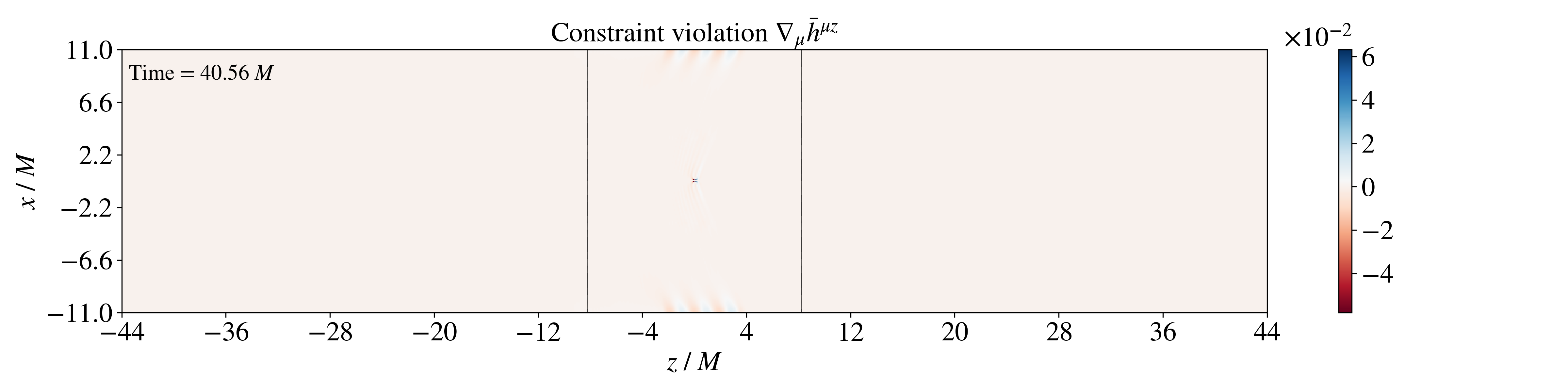
Figure 15: 2D slice of constraint violation plots at the instance when the GW is propagating inside the the NFW potential(strong gravity case with \(\phi_{\text{max}}=0.49\)). We note that at this simulation resolution considered, the constraint violation is well below the order of GW amplitude. The black outlined boxes inside the simulation domain is where the AMR patch exists and has twice the resolution of base grid.. a — Lorenz gauge violation \(C_t\), b — Lorenz gauge violation \(C_x\), c — Lorenz gauge violation \(C_y\), d — Lorenz gauge violation \(C_z\)
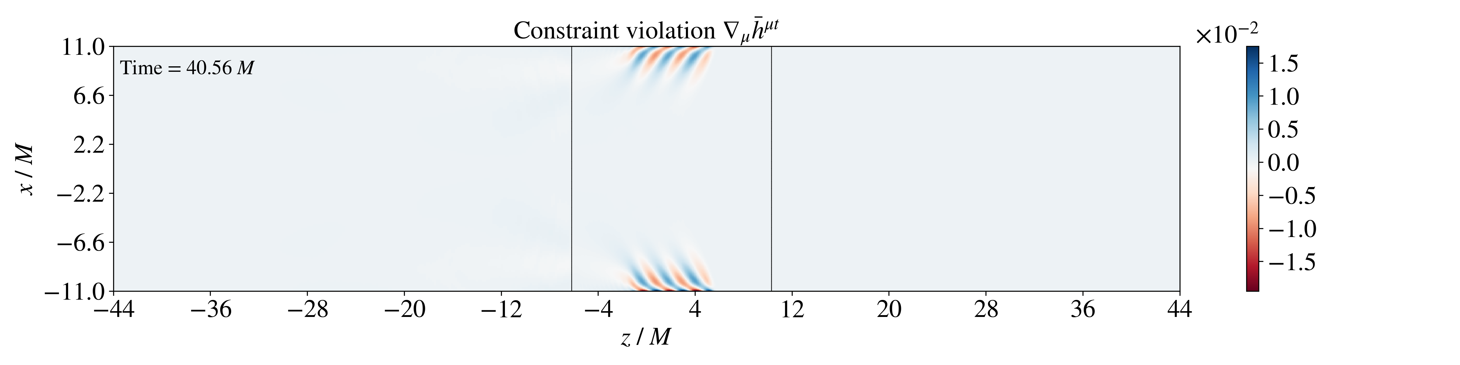

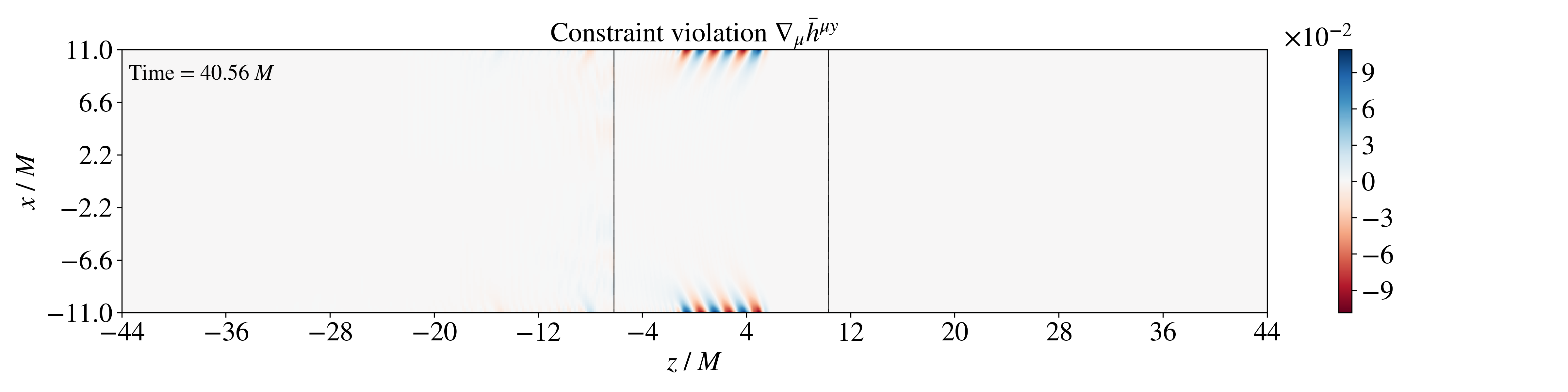
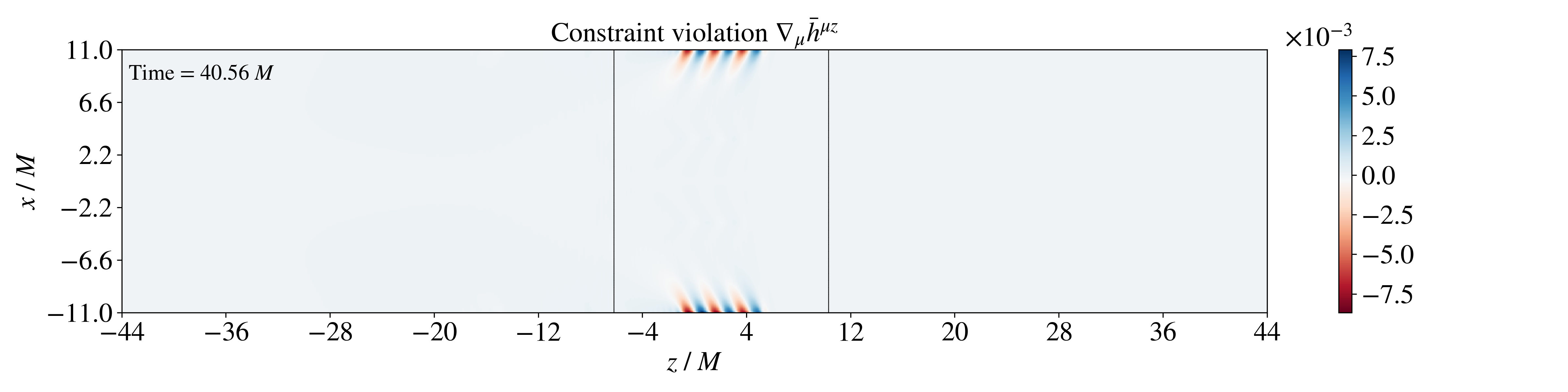
Figure 16: 2D slice of constraint violation plots at the instance when the GW is propagating inside the the Burkert potential(weak gravity case with \(\phi_{\text{max}}=0.1\)). We note that at this simulation resolution considered, the constraint violation is well below the order of GW amplitude. The black outlined boxes inside the simulation domain is where the AMR patch exists and has twice the resolution of base grid.. a — Lorenz gauge violation \(C_t\), b — Lorenz gauge violation \(C_x\), c — Lorenz gauge violation \(C_y\), d — Lorenz gauge violation \(C_z\)
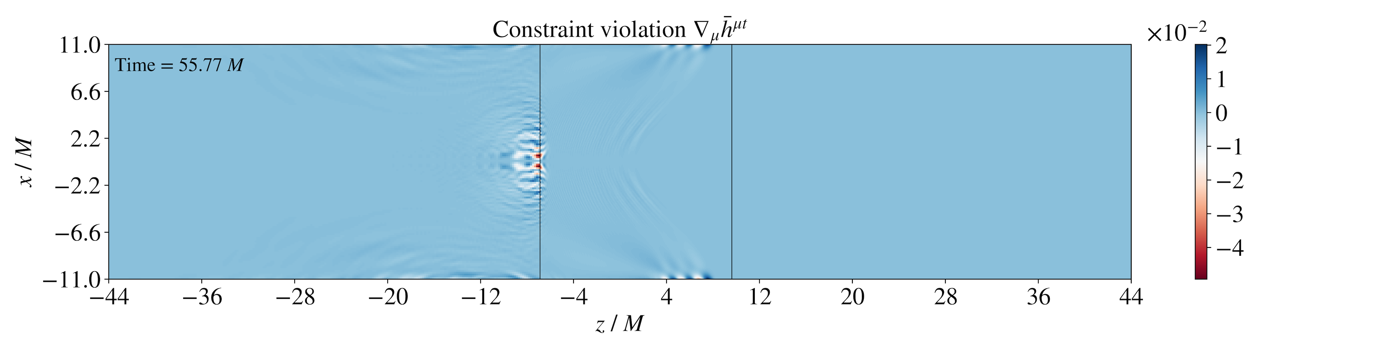
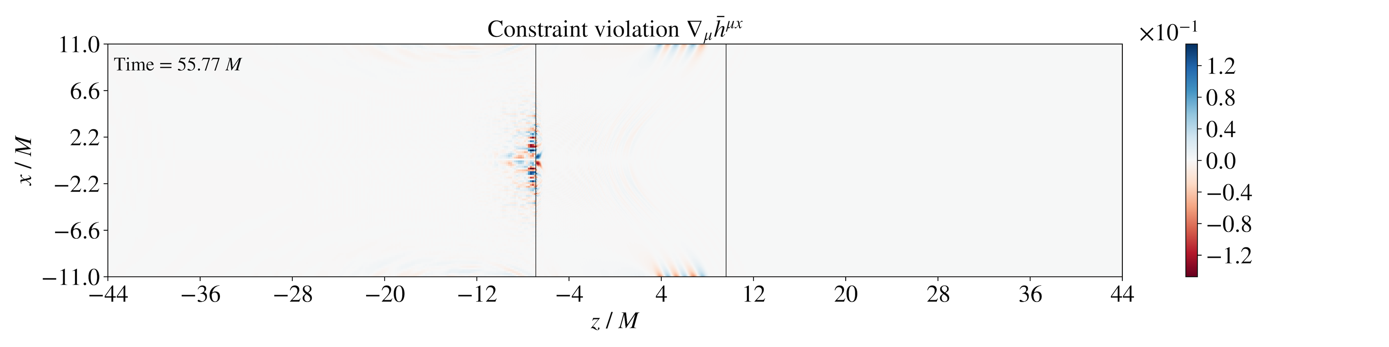

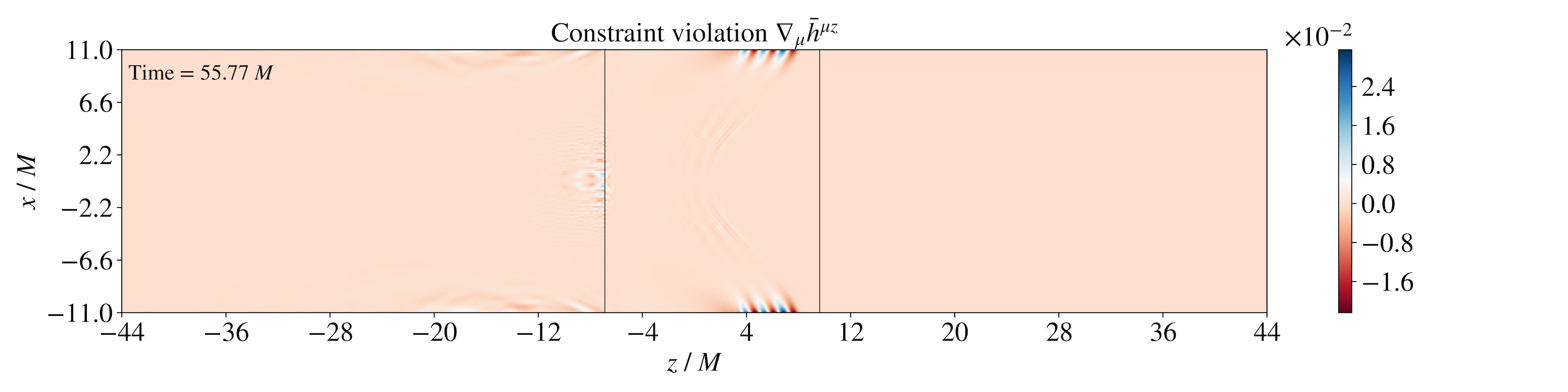
Figure 17: 2D slice of constraint violation plots at the instance when the GW is propagating inside the the Burkert potential(strong gravity case with \(\phi_{\text{max}}=0.49\)). We note that at this simulation resolution considered, the constraint violation is well below the order of GW amplitude. The black outlined boxes inside the simulation domain is where the AMR patch exists and has twice the resolution of base grid.. a — Lorenz gauge violation \(C_t\), b — Lorenz gauge violation \(C_x\), c — Lorenz gauge violation \(C_y\), d — Lorenz gauge violation \(C_z\)