I.i.d. Prophet Inequalities with Discounted Rewards: As Hard as the Non-i.i.d. Case
June 29, 2026
Abstract
We study prophet inequalities with discounted rewards, where i.i.d.base rewards are multiplicatively discounted over time. Our main message is that even this structured and arbitrarily weak form of nonstationarity can erase the classical advantage of the stationary i.i.d.setting. Focusing on single-quantile threshold policies, we show that the competitive ratio transitions from the classical \(1-1/e\) guarantee to a fundamental \(1/2\) barrier as discounting accumulates over many phases in a canonical regime with a common-decay factor and equal-length phases. We further show that, in the same regime, the \(1/2\) barrier persists even for arbitrary stopping rules. Consequently, i.i.d.base rewards under discounting can be as hard as the fully non-i.i.d. case. On the algorithmic side, we design single-quantile threshold rules that attain the tight bounds by calibrating acceptance decisions to an effective horizon induced by discounting, and we extend this calibration to heterogeneous decay factors and unequal phase lengths. We further show that a similar discontinuous breakdown persists in an infinite-horizon continuous-decay benchmark, where arbitrarily weak decay collapses the stationary benchmark from \(1\) to \(1/2\).
1 Introduction↩︎
Prophet inequalities constitute a fundamental class of problems in online optimal stopping [1]. A decision maker (the “gambler”) sequentially observes a stream of non-negative random variables (the “rewards”), revealed one at a time, and must decide at each stage whether to accept the current reward and stop or to continue observing future rewards. Performance is benchmarked against a prophet, an omniscient agent who observes all realizations in advance and can always select the maximum reward. The goal of the gambler is to design an online stopping rule whose expected payoff is competitive with that of the prophet, typically measured through the competitive ratio. Owing to their rich mathematical structure and practical relevance, prophet inequalities have been extensively studied [2] and have found applications in areas such as posted-price mechanisms [3], online advertisement allocation [4], and hiring processes in labor markets [5].
The prophet-inequalities literature has established tight constant-factor guarantees. On one side, in stationary i.i.d.reward settings, the classical \(1-1/e\) competitive-ratio bound is known to be tight for a class of single-threshold policies [2], [6]. On the other side, for independent but non-identically distributed (non-i.i.d.) reward sequences, the optimal competitive ratio degrades to \(1/2\), as shown by [7]. Despite this extensive literature, existing results largely focus on these two extreme endpoints and have not addressed structured forms of nonstationarity that interpolate between them. We study a natural mechanism to bridge between the stationary i.i.d.and fully non-i.i.d.settings: rewards are discounted with time, i.e., the scale of the reward distribution decreases over time. This framework isolates a discounting-induced transition from stationarity to nonstationarity, allowing a precise characterization of how classical guarantees break down. In particular, we show that even arbitrarily small discounting, when accumulated over long horizons, rules out any competitive ratio exceeding \(1/2\), matching the worst-case guarantee in the non-i.i.d.setting. In other words, i.i.d.prophet inequalities with slightly discounted rewards are as hard as the non-i.i.d.case.
Beyond its theoretical interest, reward decay arises naturally in many practical environments where opportunities deteriorate over time due to time preferences, depreciation, congestion effects, or market saturation [8]–[12].
We shall focus on single-quantile threshold stopping policies. Such a policy fixes an acceptance quantile in advance and accepts the first observation whose value exceeds the corresponding quantile threshold of the current reward distribution. In the stationary i.i.d.setting, this is equivalent, up to tie-breaking, to using a fixed value threshold. Under reward decay, however, fixed-value and fixed-quantile thresholds no longer coincide. We formulate our policies in terms of a fixed acceptance quantile, and refer to them as single-threshold policies throughout.
Threshold policies are a cornerstone of prophet inequalities due to their simplicity and sharp guarantees. In the stationary i.i.d.setting, single-threshold policies achieve the classical \(1-1/e\) guarantee, which is tight within that policy class [2], [6]. In the independent non-i.i.d.setting, a fixed value-threshold rule attains the optimal worst-case competitive ratio \(1/2\) [7] (see also [13], [14]). From an economic perspective, single-threshold stopping rules naturally correspond to standard posted-price mechanisms [15], in which the decision maker commits to a fixed acceptance rule in advance. Such mechanisms are appealing due to their single-parameter structure, which reduces approximation to choosing a single price and yields transparent and tractable policies [16].
As a consequence, we will study the performance of the single-threshold policies under decaying rewards and characterize their achievable competitive ratios, to answer the following natural question:
To what extent do single-threshold policies retain their classical performance guarantees under decaying rewards?
We tackle this question by identifying the fundamental performance limits and designing single-threshold algorithms that match these limits in this setting. Our main contributions are the following.
Fundamental limits under reward decay. We derive a tight worst-case upper bound for single-quantile threshold policies under decaying rewards for a common decay factor and equal-length phases. These bounds reveal a sharp transition from the classical \(1-1/e\) guarantee to a worst-case \(1/2\) barrier in the boundary regime between stationarity and discounting. This \(1/2\) barrier is worst-case optimal, matching the classical non-i.i.d. impossibility bound. We also show that the \(1/2\) barrier is not an artifact of single-threshold policies: any arbitrary stopping rules face the same worst-case barrier.
Single-threshold optimality via an effective-horizon principle. We design single-threshold algorithms that match the above upper bound for a common decay factor with equal-length phases. The key insight is an effective-horizon principle: at the level of the prophet benchmark (expected maxima), a decaying reward sequence behaves like a stationary i.i.d.sequence observed over a shorter horizon. Calibrating the acceptance quantile to this effective horizon yields tight guarantees. The same calibration extends to heterogeneous decay factors and unequal phase lengths.
Infinite-horizon continuous-decay benchmark. As a clean benchmark for the long-run effect of discounting, we study an infinite-horizon model with continuously decaying rewards. This benchmark reveals a sharp discontinuity: while the stationary infinite-horizon setting admits a trivial competitive ratio of \(1\), introducing arbitrarily weak decay induces a sharp breakdown, yielding a worst-case competitive ratio of \(1/2\). Moreover, we prove that our single-threshold rule is optimal in this benchmark and achieves this bound.
2 Related Work↩︎
The study of prophet inequalities dates back to the seminal work of [17]. Subsequent work established sharp constant-factor benchmarks in the independent non-i.i.d.and stationary i.i.d.settings. In the independent but non-identically distributed (non-i.i.d.) case, [7] showed that a threshold stopping rule attains the optimal competitive ratio of \(1/2\). In the i.i.d.setting, [18] established a competitive ratio of at least \(1-1/e\), later reinterpreted in algorithmic terms as a single-quantile threshold policy that accepts the first observation exceeding a suitable quantile [2], [13], [14]. Beyond single-threshold policies, more adaptive but computationally involved approaches have been proposed to improve performance in related settings, such as [19] and [6].
In contrast to the above literature, which primarily focuses on stationary i.i.d.rewards or fully general non-identically distributed reward sequences, our work studies single-threshold stopping policies under a discounting-induced nonstationary reward model. This framework captures a continuous transition from stationarity to reward decay, isolating the effect of discounting as a structured departure from the i.i.d.setting.
Discounting has also appeared in related prophet-region, secretary-type, and random-horizon settings. In the prophet-region literature, [20] studies uniformly bounded random variables under discounting, and characterizes the corresponding prophet regions, yielding sharp additive comparisons between the expected maximum and the optimal stopping value. In the discounted secretary problem, [21] consider random-order arrivals with time-dependent discount factors and obtain competitive guarantees for fixed sets of arbitrary values. Relatedly, [22] study i.i.d.prophet inequalities with a random horizon, where the horizon distribution is known but its realization is not; this model can be viewed through a discounted optimal stopping problem with discount factors given by the horizon survival probabilities. While these works feature discounting or horizon-induced discounting, they address different mechanisms and objectives: prophet-region/additive-gap comparisons, random-order secretary models, and uncertainty in the horizon length. In contrast, our focus is on multiplicative competitive ratios for i.i.d. draws from a base distribution under reward decay, and in particular on how structured reward decay induces a transition from the stationary i.i.d.prophet setting to non-i.i.d.-type hardness.
3 Problem Statement↩︎
We consider the classical prophet-inequality framework over a finite horizon \(n\in\mathbb{N}\), where a nonnegative random reward \(X_i\ge 0\) is revealed sequentially to a gambler at each stage \(i\in[n]\). To model decaying reward distributions, we partition the time horizon into \(S \ge 1\) consecutive phases, or time intervals, \(\{\mathcal{T}_s\}_{s=1}^S\), which form a disjoint partition of \([n]\). We denote by \(n_s := |\mathcal{T}_s|\) the length of phase \(s\), so that \(\sum_{s=1}^S n_s = n\).
Let \(Y_1,\ldots,Y_n\) be i.i.d.samples from a base reward distribution \(\mathcal{D}\) supported on \(\mathbb{R}_+\), with finite mean. Let \(\gamma_s\in[0,1]\) for all \(s\in[S-1]\) denote phase-wise decay factors, and define the cumulative decay coefficients \[\Gamma_s:=\prod_{t=1}^s \gamma_t, \quad s=1,\dots,S-1, \text{ and } \; \Gamma_0:=1.\] Then, for each phase \(s\in[S]\) and index \(i\in\mathcal{T}_s\), the observed (decayed) reward is defined as \[X_i := \begin{cases} Y_i, & s=1,\\[4pt] \Gamma_{s-1}\,Y_i, & s\ge 2, \end{cases}\] where \(\Gamma_{s-1}\) captures the cumulative decay in reward magnitude across phases.
We first analyze the canonical setting with a common decay factor and equal-length phases, where \(\gamma_s=\widetilde{\gamma}\in[0,1]\) for all \(s\in[S-1]\) and \(n_s=n/S\) for all \(s\in[S]\) (or asymptotically \(n_s/n\to 1/S\)). In this case, the observed rewards take the simple form \(X_i=\widetilde{\gamma}^{s-1}Y_i\) for \(i\in\mathcal{T}_s\). We focus on this canonical setting first because it isolates the effect of accumulated discounting in its simplest form. We later return to the general phase-dependent formulation to handle heterogeneous decay factors and unequal phase lengths.
Following most of the prior literature in prophet inequalities [6], [7], [13], [14], [18], we assume that the reward distributions are known, which corresponds to knowing the base distribution \(\mathcal{D}\), as well as the phase partition \(\{\mathcal{T}_s\}_{s\in[S]}\) and decay factors \((\gamma_s)_{s\in[S-1]}\) in advance.
3.0.0.1 Stopping rule.
At each stage \(i\), after observing \(X_i\), the decision maker must either stop and accept the current reward or continue to the next stage, thereby irrevocably forfeiting the option to stop at any earlier stage. A stopping rule (or policy) \(\tau\) is a random variable taking values in \(\{1,2,\ldots,n\}\cup\{n+1\}\) such that \(\tau\) is a stopping time with respect to the natural filtration generated by \((X_i)_{i\ge1}\). The value \(\tau = n+1\) corresponds to the event that no reward is accepted within the horizon, in which case the payoff is defined to be zero. The expected reward of a policy \(\tau\) is given by \[\mathbb{E}[X_\tau] = \sum_{i=1}^{n} \mathbb{E}[X_i \,\mathbb{1}\{\tau = i\}].\]
3.0.0.2 Prophet benchmark and competitive ratio.
We compare the performance of an online stopping rule \(\tau\) with that of a prophet who knows all realizations \(\{X_1, \ldots, X_n\}\) in advance and can always select the maximum reward. The prophet’s expected reward is therefore \[\mathbb{E}\!\left[\max_{i \in [n]} X_i\right].\] The performance of a stopping policy \(\tau\) is measured by its competitive ratio (CR) in the decay rewards with horizon \(n\), which is defined as \[\mathrm{CR}_n(\tau) = \frac{\mathbb{E}[X_\tau]}{\mathbb{E}\!\left[\max_{i \in [n]} X_i\right]}.\] The quantity \(\mathrm{CR}_n(\tau)\) implicitly depends on the decay profile, the phase partition, and the base distribution; we suppress this dependence to keep the notation light. We seek stopping policies that maximize \(\mathrm{CR}_n(\tau)\) uniformly over the class of base reward distributions \(\mathcal{D}\).
3.0.0.3 Quantile rather than value thresholds.
Throughout the paper, we focus on single-quantile threshold policies. This choice is natural under reward decay because a fixed quantile of the reward distribution induces phase-dependent value thresholds that scale with the discount factors. In particular, if the first-phase threshold is \(\alpha_1\), then the corresponding threshold in phase \(s+1\) is obtained simply as \[\alpha_{s+1}=\gamma_s\alpha_s .\] Thus single-quantile thresholds retain the same one-parameter simplicity and online implementation cost as static value thresholds.
Single-quantile and single-value threshold policies have comparable implementation cost, and in the stationary i.i.d.setting they coincide up to tie-breaking. Under reward decay, however, this equivalence breaks down: a single fixed value threshold is not invariant to the changing reward scale and can be strictly suboptimal. Appendix 10.1 provides a separating example showing that, even with a common decay factor and equal-length phases, single-value thresholds cannot attain the single-quantile benchmark characterized below. Henceforth, we focus on single-quantile threshold policies, which we refer to simply as single-threshold policies.
4 Fundamental Limits in the Canonical Decay Model↩︎
We begin with the canonical case of a common decay factor \(\gamma_s=\widetilde{\gamma}\) for all \(s\in[S-1]\) and equal asymptotic phase lengths, \(n_s=n/S\) for all \(s\in[S]\). For simplicity, we assume that \(S\) divides \(n\). This symmetric setting captures the central phenomenon: accumulated discounting can drive the competitive ratio from the classical i.i.d.value \(1-1/e\) down to the non-i.i.d.barrier \(1/2\).
Theorem 1. Consider the setting with a common decay factor and equal-length phases described above. There exists a family of decaying reward distributions such that for any single-threshold stopping policy \(\tau\), the competitive ratio satisfies \[\limsup_{n\to\infty}\mathrm{CR}_n(\tau) \;\le\; \begin{cases} \displaystyle \frac{\big(1-\widetilde{\gamma}^{S}\exp\!\big(-S\tfrac{1-\widetilde{\gamma}}{1-\widetilde{\gamma}^{S}}\big)\big) \big(1-\exp\!\big(-\tfrac{1-\widetilde{\gamma}}{1-\widetilde{\gamma}^{S}}\big)\big)}{1-\widetilde{\gamma}\,\exp\!\big(-\tfrac{1-\widetilde{\gamma}}{1-\widetilde{\gamma}^{S}}\big)}, & \text{if } \; 0 \le \widetilde{\gamma} < 1, \\[12pt] 1 - \tfrac{1}{e}, & \text{if }\; \widetilde{\gamma} = 1. \end{cases}\]
Proof Sketch. Here we provide a proof sketch and the full version is provided in Appendix 10.2. The key is to construct a single hard distribution, depending only on \((S,\widetilde{\gamma})\), that upper bounds every single-threshold policy.
4.0.0.1 Step 1: Hard instance and prophet benchmark.
Let the phases have equal length \(n/S\), and consider \[Y_i= \begin{cases} n, & \text{with probability }1/n^2,\\ y_{\widetilde{\gamma}}, & \text{with probability }1-1/n^2, \end{cases} \qquad X_i=\widetilde{\gamma}^{s-1}Y_i,\quad i\in\mathcal{T}_s,\] where the constant \(y_{\widetilde{\gamma}}\ge 0\) will be chosen below. Define \[c_{\widetilde{\gamma}}:=\frac{1}{S}\sum_{s=1}^S\widetilde{\gamma}^{s-1} = \begin{cases} \dfrac{1-\widetilde{\gamma}^S}{S(1-\widetilde{\gamma})},&0\le\widetilde{\gamma}<1,\\[6pt] 1,&\widetilde{\gamma}=1. \end{cases}\] Then we show that \[\mathbb{E}\!\left[\max_{i\in[n]}X_i\right] =y_{\widetilde{\gamma}}+c_{\widetilde{\gamma}}+o(1).\]
4.0.0.2 Step 2: Upper bound for an arbitrary threshold.
A single-quantile threshold is characterized by a per-stage acceptance probability \(p\). If \(R_s(p)\) is the expected reward conditional on acceptance in phase \(s\), then we show that, uniformly in \(p\), \[pR_s(p) \le \frac{\widetilde{\gamma}^{s-1}}{n} +\widetilde{\gamma}^{s-1}y_{\widetilde{\gamma}} p.\] Consequently, \[\mathbb{E}[X_\tau]=\sum_{s=1}^S\sum_{i\in\mathcal{T}_s} p\,R_{s}(p)\,(1-p)^{i-1} \le \sum_{s=1}^S \left(\frac{\widetilde{\gamma}^{s-1}}{n} +\widetilde{\gamma}^{s-1}y_{\widetilde{\gamma}} p\right) (1-p)^{(s-1)n/S} \frac{1-(1-p)^{n/S}}{p}.\] Writing \(x=np\), for every fixed \(x>0\) this yields \[\mathbb{E}[X_\tau] \le \left(\frac{1}{x}+y_{\widetilde{\gamma}}\right)A_S(x)+o(1),\] where \[A_S(x):= \sum_{s=1}^S \widetilde{\gamma}^{s-1}e^{-(s-1)x/S}(1-e^{-x/S}) = \frac{(1-\widetilde{\gamma}^S e^{-x})(1-e^{-x/S})}{1-\widetilde{\gamma} e^{-x/S}}.\] Thus \[\mathrm{CR}_n(\tau) \le f_S(x,y_{\widetilde{\gamma}})+o(1), \qquad f_S(x,y):= \frac{(\frac{1}{x}+y)A_S(x)}{y+c_{\widetilde{\gamma}}}.\]
4.0.0.3 Step 3: Choosing a fixed hard value \(y_{\widetilde{\gamma}}\).
Set \[x_{\widetilde{\gamma}}:=\frac{1}{c_{\widetilde{\gamma}}}\] and define \[y(x):=\frac{A_S(x)}{x^2A_S'(x)}-\frac{1}{x}, \qquad y_{\widetilde{\gamma}}:=y(x_{\widetilde{\gamma}}).\] We show that, for \(y_{\widetilde{\gamma}}=y(x_{\widetilde{\gamma}})\), \(f_S(\cdot,y_{\widetilde{\gamma}})\) is increasing before \(x_{\widetilde{\gamma}}\) and decreasing after \(x_{\widetilde{\gamma}}\). Hence \[\sup_{x\in[0,\infty]}f_S(x,y_{\widetilde{\gamma}}) =f_S(x_{\widetilde{\gamma}},y_{\widetilde{\gamma}}) =A_S(x_{\widetilde{\gamma}}),\] where the last equality follows from \(1/x_{\widetilde{\gamma}}=c_{\widetilde{\gamma}}\). Thus the single choice \(y_{\widetilde{\gamma}}\) defeats every single threshold.
4.0.0.4 Step 4: Evaluation.
For \(0\le\widetilde{\gamma}<1\), \[x_{\widetilde{\gamma}}=\frac{S(1-\widetilde{\gamma})}{1-\widetilde{\gamma}^S},\] and hence \[A_S(x_{\widetilde{\gamma}}) = \frac{ \left(1-\widetilde{\gamma}^S \exp\!\left(-S\frac{1-\widetilde{\gamma}}{1-{\widetilde{\gamma}}^S}\right)\right) \left(1- \exp\!\left(-\frac{1-\widetilde{\gamma}}{1-{\widetilde{\gamma}}^S}\right)\right)}{1-\widetilde{\gamma} \exp\!\left(-\frac{1-\widetilde{\gamma}}{1-{\widetilde{\gamma}}^S}\right)}.\] When \(\widetilde{\gamma}=1\), we have \(x_{\widetilde{\gamma}}=1\) and \(A_S(1)=1-1/e\). Therefore, \[\limsup_{n\to\infty}\mathrm{CR}_n(\tau) \le A_S(x_{\widetilde{\gamma}}),\] which is the claimed bound. ◻
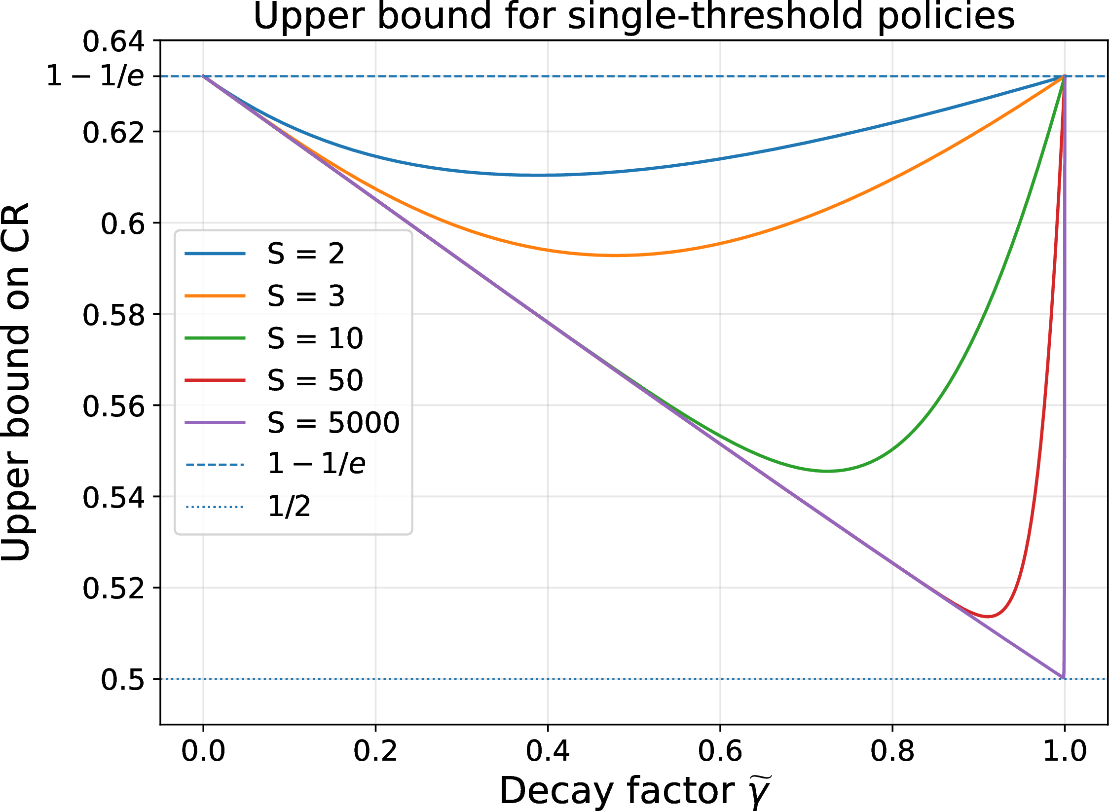
Figure 1 plots the upper bound in Theorem 1 as a function of the decay factor \(\widetilde{\gamma}\) for several values of \(S\). For fixed \(S\), the bound recovers the classical value \(1-1/e\) at the stationary point \(\widetilde{\gamma}=1\) and 3\(\widetilde{\gamma}=0\). However, as \(S\) grows, the worst-case guarantee deteriorates in the near-stationary regime \(\widetilde{\gamma} \to 1\), and the minimum approaches the \(1/2\) barrier. The following corollary makes this convergence to the \(1/2\) barrier explicit.
Corollary 1 (Worst-case asymptotics). Under the assumptions of Theorem 1, let \(U_S(\widetilde{\gamma})\) denote the upper-bound value in Theorem 1. Then, for every fixed \(\widetilde{\gamma}\in[0,1)\), \[\lim_{S\to\infty} U_S(\widetilde{\gamma}) = \frac{1-\exp(-(1-\widetilde{\gamma}))}{1-\widetilde{\gamma}\exp(-(1-\widetilde{\gamma}))} =:U_\infty(\widetilde{\gamma}).\] Moreover, \(U_\infty(\widetilde{\gamma})\) is non-increasing on \([0,1)\) and satisfies \[\lim_{\widetilde{\gamma}\uparrow 1} U_\infty(\widetilde{\gamma}) = \frac{1}{2} .\] Equivalently, the same conclusion holds along any joint limit \(S\to\infty\) and \(\widetilde{\gamma}\uparrow1\) such that \(\widetilde{\gamma}^{S}\to 0\) (i.e., \(S(1-\widetilde{\gamma})\to\infty\)).
4.0.0.5 Discontinuous breakdown at the stationarity boundary
Under \(S\to \infty\), the regime \(\widetilde{\gamma} \uparrow 1\) corresponds to the boundary between stationary and decay reward sequences. Over short time scales, the reward process is nearly indistinguishable from the i.i.d.case, while over long horizons the cumulative effect of decay becomes significant. At this boundary, the algorithm faces the sharpest trade-off: waiting is tempting because over short horizons the process looks nearly i.i.d., but waiting is expensive because over long horizons the cumulative decay becomes substantial. This trade-off is reflected in the worst-case bound, whose limiting value approaches \(1/2\) as \(\widetilde{\gamma}\uparrow 1\) under \(S\to\infty\). Thus the boundary regime exhibits a discontinuous breakdown from the stationary value \(1-1/e\) attained at \(\widetilde{\gamma}=1\) (see the case (S=10000) in Figure 1).
This observation raises two natural questions. First, is this upper bound tight within the class of single-threshold policies? Second, is the resulting \(1/2\) limit merely an artifact of the single-threshold restriction, or is it an intrinsic limitation of the discounted-reward model? The next section answers the first question by giving a matching effective-horizon threshold rule; we return to the second question later by analyzing the optimal dynamic-programming policy.
5 Single-Threshold Algorithm for the Canonical Decay Model↩︎
In this section, we present a single-quantile threshold algorithm that achieves tight competitive ratios for a common decay factor with \(\widetilde{\gamma}\) and equal asymptotic phase lengths with \(n_s=n/S\). Both the design of the algorithm and its analysis are calibrated through the notion of an effective horizon: \[B := \sum_{s=1}^{S} \widetilde{\gamma}^{s-1}\, \frac{n}{S},\] which aggregates the total discounted mass of opportunities across all phases.
The central insight underlying our analysis is an effective-horizon principle: in terms of expected maxima, the prophet benchmark under decay is bounded above by that of a stationary i.i.d.sequence observed over an effective horizon of length \(B\). We begin by formalizing this intuition through a key comparison lemma, which plays a crucial role in both the calibration of the acceptance threshold and the ensuing competitive-ratio analysis.
5.1 Bounding the Expected Maximum↩︎
We bound the prophet’s expected maximum in terms of an effective horizon. The proof is deferred to Appendix 10.3.
Lemma 1. Let \(F\) denote the cumulative distribution function of the base reward distribution \(\mathcal{D}\). Consider a common decay factor and equal-length phases. Then, we have \[\label{eq:multistage} \int_0^\infty \Bigl(1-F(z)^{B}\Bigr)\,dz \;\ge\; \int_0^\infty \Bigl(1-\prod_{s=1}^{S} F\!\bigl(z/\widetilde{\gamma}^{\,s-1}\bigr)^{n/S}\Bigr)\,dz,\qquad{(1)}\] where we adopt the convention \(F(z/0):=\lim_{u\to\infty}F(u)=1\) for \(z\ge0\).
We now explain the implication of the preceding lemma. For each \(i\in\mathcal{T}_s\), the cumulative distribution function of \(X_i\) is \(z\mapsto F\!\bigl(z/\widetilde{\gamma}^{s-1}\bigr)\). Combining this with the standard survival-function formula for maxima yields \[\mathbb{E}\!\left[\max_{i \in [B]} Y_i\right] =\int_0^\infty \bigl(1-F(z)^{B}\bigr)\,dz \;\ge\; \int_0^\infty \Bigl(1-\prod_{s=1}^{S} F\!\bigl(z/\Gamma_{s-1}\bigr)^{n/S}\Bigr)\,dz =\mathbb{E}\!\left[\max_{i \in [n]} X_i\right],\] where, for notational simplicity, we assume \(B\in\mathbb{N}\). This inequality identifies \(B\) as an effective horizon for the prophet benchmark (expected maxima). We use it to calibrate the acceptance quantile and to analyze the competitive ratio.
5.2 Single-Threshold Policy↩︎
We consider a single-quantile stopping rule whose acceptance threshold adapts to the nonstationary scaling of the reward distribution. Let \(Y \sim \mathcal{D}\) denote a random variable drawn from the base reward distribution. For each phase \(s \in [S]\), corresponding to time indices \(i \in \mathcal{T}_s,\) the algorithm employs a phase-specific threshold \(\alpha_s\) satisfying \[\begin{align} \mathbb{P}(X_i > \alpha_s)=\mathbb{P}(\widetilde{\gamma}^{s-1} Y > \alpha_s) = \frac{a}{n},\label{eq:threshold} \end{align}\tag{1}\] where the parameter \(a\) determines the acceptance quantile and is set as the inverse of average effective decay weight across all phases as follows: \[a =\frac{1}{(1/S)+\sum_{s=1}^{S-1}(1/S) \widetilde{\gamma}^s}.\] Importantly, the thresholds satisfy the simple recursion such that for \(s\in[S-1]\) \[\alpha_{s+1}=\widetilde{\gamma}\alpha_s.\] Given the initial threshold \(\alpha_1\), this recursion allows efficient updates of the thresholds across phases. The pseudo-code of the threshold policy is provided in Algorithm 2.
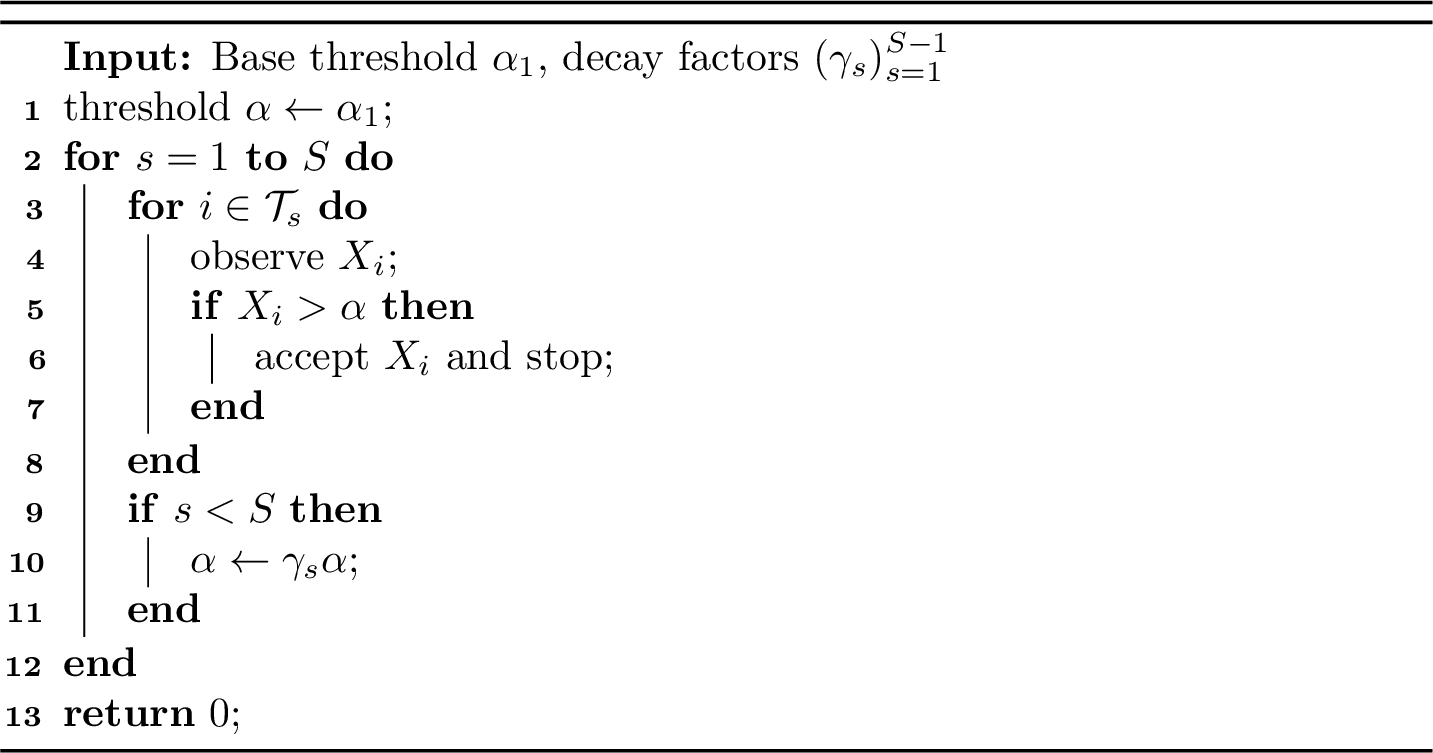
Remark 2 (Interpretation of the threshold choice). As shown in Lemma 1, the decaying reward sequence can be interpreted, in terms of expected maxima, as a stationary i.i.d.sequence with effective horizon length \(B=(1+\sum_{s=1}^{S-1}\widetilde{\gamma}^{s})\frac{n}{S}\). Accordingly, a natural acceptance quantile is \(1/B\), mirroring the classical calibration in stationary i.i.d.prophet problems where the acceptance probability scales as \(1/n\) [2]. This leads precisely to the choice \(a/n\) in 1 .
Remark 3 (Atomic base distributions). If the distribution of \(X_i=\widetilde{\gamma}^{\,s-1}Y_i\) has atoms, the strict threshold equation in 1 may fail to admit a solution due to discontinuities of the tail distribution. Following [13], [14], one may use a generalized quantile \(\alpha_s\) satisfying \[\mathbb{P}(X_i>\alpha_s)\le \frac{a}{n}\le \mathbb{P}(X_i\ge \alpha_s),\] and implement randomized tie-breaking at \(\alpha_s\) so that the acceptance probability is exactly \(\mathbb{P}(A_i)=a/n\), where \(A_i\) denotes the acceptance event at time \(i\). With this modification, the algorithm behaves as in the continuous case, and all analytical arguments go through unchanged by replacing \(\mathbb{1}\{X_i>\alpha_s\}\) with \(\mathbb{1}\{A_i\}\).
Under this construction, we obtain the following lower bound on the competitive ratio, which is tight and matches the upper bound in Theorem 1.
Theorem 4. Consider any decaying reward distributions with \(S \ge 1\) nonstationary phases of equal length and a common decay factor \(\gamma_t \equiv \widetilde{\gamma}\) for all \(t \in [S-1]\). Then, the stopping policy \(\tau\) of Algorithm 2 with \(\alpha_1\) from 1 achieves a competitive ratio bound of \[\liminf_{n\to\infty}\mathrm{CR}_n(\tau)\ge \begin{cases} \displaystyle \frac{\big(1-\widetilde{\gamma}^{S}\exp\!\big(-S\tfrac{1-\widetilde{\gamma}}{1-\widetilde{\gamma}^{S}}\big)\big) \big(1-\exp\!\big(-\tfrac{1-\widetilde{\gamma}}{1-\widetilde{\gamma}^{S}}\big)\big)}{1-\widetilde{\gamma}\,\exp\!\big(-\tfrac{1-\widetilde{\gamma}}{1-\widetilde{\gamma}^{S}}\big)}, & \text{if }\; 0 \le \widetilde{\gamma} < 1,\\[12pt] 1 - \tfrac{1}{e}, & \text{if }\; \widetilde{\gamma} = 1. \end{cases}\]
Proof Sketch. Here we provide a proof sketch, and the full version is provided in Appendix 10.4. The proof has two main components: (i) compute the expected reward of the phase-dependent threshold policy, and (ii) relate the truncated tail expectation \(B\,\mathbb{E}[Y\mathbb{1}\{Y>\alpha_1\}]\) to the prophet benchmark \(\mathbb{E}[\max_{i\in[n]}X_i]\).
5.2.0.1 Step 1: Expand \(\mathbb{E}[X_\tau]\) via the first acceptance time.
Define \(p:=\mathbb{P}(Y>\alpha_1)=a/n\). Since \(X_i>\alpha_s \iff Y_i>\alpha_1\), the acceptance events are identical across phases. By independence, \[\mathbb{E}[X_\tau] =\sum_{s=1}^S\sum_{i\in\mathcal{T}_s}\mathbb{E}\!\left[X_i\mathbf{1}\{X_i>\alpha_s\}\right](1-p)^{i-1}.\]
5.2.0.2 Step 2: Factor out the common tail moment.
For \(i\in\mathcal{T}_s\) we have \[\mathbb{E}\!\left[X_i\mathbf{1}\{X_i>\alpha_s\}\right] =\widetilde{\gamma}^{\,s-1}\mathbb{E}\!\left[Y\mathbf{1}\{Y>\alpha_1\}\right].\] Substituting into the expansion yields \[\mathbb{E}[X_\tau] =\mathbb{E}\!\left[Y\mathbf{1}\{Y>\alpha_1\}\right] \sum_{s=1}^S \widetilde{\gamma}^{\,s-1}\sum_{i\in\mathcal{T}_s}(1-p)^{i-1}.\]
5.2.0.3 Step 3: Evaluate geometric sums.
Using the above results and the geometric-series identity give the closed form \[\begin{align} \mathbb{E}[X_\tau] = \left(1-(1-a/n)^{n/S}\right) \left(1+\sum_{s=2}^S (1-a/n)^{(s-1)n/S}\widetilde{\gamma}^{s-1}\right) \,\frac{n}{a}\mathbb{E}[Y\mathbb{1}\{Y>\alpha_1\}].\label{eq:exp95reward} \end{align}\tag{2}\]
5.2.0.4 Step 4: Lower bound \(\mathbb{E}[Y\mathbb{1}\{Y>\alpha_1\}]\) by the prophet.
From the definition, \(B=\frac{n}{S}\bigl(1+\sum_{s=1}^{S-1}\widetilde{\gamma}^s\bigr)\). By Lemma 1 and the standard survival-function formula for maxima, one has the comparison \[\mathbb{E}\Big[\max_{i\in[B]}Y_i\Big]\;\ge\;\mathbb{E}\Big[\max_{i\in[n]}X_i\Big].\] It remains to relate \(\mathbb{E}[\max_{i\in[B]}Y_i]\) to the tail moment \(\mathbb{E}[Y\mathbb{1}\{Y>\alpha_1\}]\) in 2 . Using a standard truncation argument (details omitted) and \(\mathbb{P}(Y>\alpha_1)=a/n=1/B\), we obtain \[\begin{align} B\mathbb{E}[Y\mathbb{1}(Y>\alpha_1)]=\alpha_1+B\mathbb{E}[(Y-\alpha_1)_+]\ge \mathbb{E}\left[\max_{i\in[B]}Y_i\right] \ge \mathbb{E}\left[\max_{i\in [n]}{X_i}\right]. \raisetag{4ex}\label{eq:lower95bd95bE} \end{align}\tag{3}\]
5.2.0.5 Step 5: Plug in and take \(n\to\infty\).
From \(n/a=B\), 2 together with 3 gives \[\begin{align} \label{eq:lower95X95tau} \mathbb{E}[X_\tau] \;\ge\; \left(1-(1-a/n)^{n/S}\right) \left(1+\sum_{s=1}^{S-1}(1-a/n)^{sn/S}\widetilde{\gamma}^s\right) \, \mathbb{E}\Big[\max_{i\in[n]}X_i\Big]. \end{align}\tag{4}\] Letting \(n\to\infty\) leads to the explicit lower bound on the competitive ratio with \[(1-a/n)^{s(n/S)}\;\longrightarrow \;e^{-sa/S}.\] For \(0\le\widetilde{\gamma}<1\), with \(a =\frac{S(1-\widetilde{\gamma})}{1-\widetilde{\gamma}^{S}}\), 4 simplifies to \[\liminf_{n\to\infty}\mathrm{CR}_n(\tau)\;\ge\; \frac{\bigl(1-\widetilde{\gamma}^{S}e^{-S(1-\widetilde{\gamma})/(1-\widetilde{\gamma}^S)}\bigr)\bigl(1-e^{-(1-\widetilde{\gamma})/(1-\widetilde{\gamma}^S)}\bigr)}{1-\widetilde{\gamma} e^{-(1-\widetilde{\gamma})/(1-\widetilde{\gamma}^S)}},\] and for \(\widetilde{\gamma}=1\), with \(B=n\), 4 reduces to the classical \(1-1/e\) bound. ◻
Combining Theorems 1 and 4, we obtain a tight characterization of the optimal single-threshold guarantee in the canonical common-decay, equal-length setting. In particular, the effective-horizon threshold rule exactly matches the worst-case upper bound, and hence the deterioration toward \(1/2\) cannot be improved within the single-threshold class.
This naturally raises a more structural question. Is the \(1/2\) limit caused by the simplicity of single-threshold policies, or is it an intrinsic limitation of the discounted-reward model itself? We next show that the latter is the case: even the optimal dynamic-programming policy, and therefore any stopping rule, faces the same worst-case \(1/2\) barrier in the near-stationary long-phase regime.
6 The \(1/2\) Barrier Beyond Single-Threshold Policies↩︎
We now show that the \(1/2\) worst-case limit is not an artifact of restricting attention to single-threshold policies. The proof analyzes the optimal dynamic-programming (DP) policy in the common-decay, equal-length setting. Since the DP policy dominates every admissible stopping rule, an upper bound on its competitive ratio immediately yields a fundamental limitation for all stopping rules. The detailed proof is provided in Appendix 10.6.
Theorem 5 (Dynamic Programming: Worst-Case Asymptotics). Consider the setting with a common decay factor \(\widetilde{\gamma}\in[0,1)\) and equal-length phases. As \(n \to \infty\), there exists a family of decaying reward distributions such that the optimal dynamic programming policy \(\tau_{\mathrm{DP}}\) satisfies the following upper bound on the competitive ratio: in a joint limit \(\widetilde{\gamma}\uparrow 1\), and \(S \to \infty\) such that \(\widetilde{\gamma}^{S}\to 0\) (equivalently, \(S(1-\widetilde{\gamma})\to\infty\)), \[\mathrm{CR}_n(\tau_{\mathrm{DP}}) \;\longrightarrow\; \frac{1}{2}.\] Consequently, since \(\tau_{\mathrm{DP}}\) is optimal among all stopping rules, there exists a family of decaying reward distributions such that, for any stopping policy \(\tau\), \[\limsup_{n\to\infty}\mathrm{CR}_n(\tau) \;\le\; \limsup_{n\to\infty}\mathrm{CR}_n(\tau_{\mathrm{DP}}) \;\xrightarrow[\widetilde{\gamma}\uparrow 1,\; S\to\infty\;\text{s.t.}\;\widetilde{\gamma}^{S}\to 0]{}\; \frac{1}{2}.\]
6.0.0.1 Structural implication.
Theorem 5 identifies a fundamental worst-case limitation of \(1/2\) in the presence of decaying rewards. Interestingly, this \(1/2\) barrier coincides with the classical impossibility bound for prophet inequalities under arbitrary (non-identical) reward distributions [7]. This suggests that, in the boundary regime between stationarity and nonstationarity induced by decaying rewards (\(S \to \infty\), \(\gamma\to 1\)), the stopping problem can be as hard as the fully general non-identically distributed setting.
Having established that the \(1/2\) barrier persists beyond single-threshold rules in this symmetric phase setting, we now return to single-threshold policies and show that the effective-horizon calibration extends beyond the symmetric case to heterogeneous decay factors and unequal phase lengths.
7 Extension to General Decay Factors and Phase Lengths↩︎
The common-decay, equal-length setting makes the effective-horizon principle transparent: discounting reduces the total effective mass of opportunities, and the appropriate acceptance quantile should be calibrated to this discounted horizon rather than to the raw horizon. We now show that the same idea extends to heterogeneous phase profiles.
Specifically, we allow the phase-wise discount factors to vary arbitrarily, with \(\gamma_s\in[0,1]\) for \(s\in[S-1]\), and allow the phase lengths \(n_s\) to vary across phases, assuming that each phase occupies a nonvanishing asymptotic fraction of the horizon. Formally, there exist phase proportions \(\lambda_1,\dots,\lambda_S\in(0,1]\), with \(\sum_{s=1}^S\lambda_s=1\), such that, as \(n\to\infty\), \[\frac{n_s}{n}\to \lambda_s, \qquad s\in[S].\] In this setting, the contribution of each phase is determined by two quantities: its relative length \(\lambda_s\), and its cumulative reward scale \(\Gamma_{s-1}\). Accordingly, define \[\Lambda_{s-1}:=\sum_{t=1}^{s-1}\lambda_t \quad (\Lambda_0:=0), \qquad C_S:=\sum_{t=1}^S\Gamma_{t-1}\lambda_t.\] We also define the effective horizon as \[B_G:=\sum_{s=1}^{S}\Gamma_{s-1}n_s .\] The effective-horizon comparison for expected maxima in Lemma 1 extends to this generalized horizon \(B_G\) (Appendix 10.3). Moreover, since \(B_G/n\to C_S\), the quantity \(C_S\) can be viewed as the normalized effective horizon associated with the heterogeneous phase profile.
7.0.0.1 Fundamental Limits.
We first investigate the fundamental limitations of single-threshold stopping policies under this generalized phase profile. The following theorem shows that the upper-bound expression from the case of common decay and equal-length phases extends directly once each phase is weighted by its length and cumulative discount. The proof is deferred to Appendix 10.5.
Theorem 6. Fix any \(S\ge 1\), decay factors \((\gamma_s)_{s=1}^{S-1}\in[0,1]^{S-1}\), and phase proportions \((\lambda_s)_{s=1}^S\in(0,1]^S\) with \(\sum_{s=1}^S\lambda_s=1\). For any single-threshold stopping policy \(\tau\), whose acceptance quantile is independent of the base distribution, there exists a family of decaying reward distributions such that \[\limsup_{n\to\infty}\mathrm{CR}_n(\tau) \le \sum_{s=1}^S \Gamma_{s-1} \exp\left(-\frac{\Lambda_{s-1}}{C_S}\right) \left(1 - \exp\left(-\frac{\lambda_s}{C_S}\right)\right).\]
The expression in Theorem 6 has a direct phase-by-phase interpretation. Under the effective-horizon calibration, the probability of reaching phase \(s\) is asymptotically \[\exp\left(-\frac{\Lambda_{s-1}}{C_S}\right),\] while the probability of accepting within phase \(s\), conditional on reaching it, is \[1-\exp\left(-\frac{\lambda_s}{C_S}\right).\] Multiplying these terms by the reward scale \(\Gamma_{s-1}\) and summing over phases gives exactly the right-hand side of the theorem. Thus the upper bound already suggests the right algorithmic calibration: the acceptance quantile should be set according to the total discounted opportunity mass, rather than the raw horizon length.
This formula recovers the earlier canonical setting as a special case. In particular, under a common decay factor and equal-length phases, i.e., \(\Gamma_{s-1}=\widetilde{\gamma}^{s-1}\) and \(\lambda_s=1/S\), it reduces to the bound derived for the common-decay, equal-length model in Theorem 1.
7.0.0.2 Tightness via Effective-Horizon Calibration.
The preceding interpretation leads to the matching threshold rule. Since \(B_G=\sum_{s=1}^{S}\Gamma_{s-1}n_s\) is the effective number of discounted opportunities, the natural analogue of the classical \(1/n\)-quantile rule is a \(1/B_G\)-quantile rule. For each phase \(s\in[S]\), choose the threshold \(\alpha_s\) so that \[\begin{align} \mathbb{P}(\Gamma_{s-1}Y>\alpha_s) = \frac{\widetilde{a}}{n}, \text{ where } \widetilde{a}=\frac{1}{(n_1/n)+\sum_{t=1}^{S-1}(n_{t+1}/n)\Gamma_t}. \label{eq:threshold95gen} \end{align}\tag{5}\] This calibration satisfies \({\widetilde{a}}/{n} = {1}/{B_G}\) and \(\widetilde{a}\to 1/C_S\). Thus the policy uses the same one-parameter quantile rule as in the symmetric case, but expressed in the correct effective time scale.
Theorem 7. Consider the decaying-reward model with \(S\ge1\) phases, decay factors \((\gamma_s)_{s=1}^{S-1}\in[0,1]^{S-1}\), and phase proportions \((\lambda_s)_{s=1}^{S}\in(0,1]^S\) with \(\sum_{s=1}^S\lambda_s=1\). Then Algorithm 2, with thresholds defined by 5 , satisfies \[\liminf_{n\to\infty}\mathrm{CR}_n(\tau)\ge \sum_{s=1}^S \Gamma_{s-1} \exp\left(-\frac{\Lambda_{s-1}}{C_S}\right) \left(1-\exp\left(-\frac{\lambda_s}{C_S}\right)\right),\] where \(\Lambda_{s-1}:=\sum_{t=1}^{s-1}\lambda_t\) with \(\Lambda_0:=0\).
Combining Theorems 6 and 7, we obtain a characterization of the optimal single-threshold guarantee in the general phase-dependent setting. Heterogeneous decay factors and unequal phase lengths do not require a fundamentally different policy; they only modify the effective horizon and the phase-by-phase weights. We conclude the theoretical analysis by considering a complementary infinite-horizon benchmark, which illustrates the long-run effect of discounting beyond the finite-horizon single-threshold setting.
8 Infinite-Horizon Continuous Decay (\(S=n=\infty\))↩︎
As a clean benchmark for the long-run effect of discounting, we turn to an infinite-horizon model with continuous decay, corresponding to the regime \(S=n=\infty\). Whereas the preceding results characterize large-\(n\) limits for finite horizons, this benchmark provides a discounted setting in which the same \(1/2\) barrier persists. In the infinite-horizon setting, a stopping rule \(\tau\) is a stopping time taking values in \(\mathbb{N}\cup\{\infty\}\), where \(\tau=\infty\) denotes never stopping.
Theorem 8. Consider the continuous decay regime with an infinite sequence of phases (\(S=n=\infty\)) and a common decay factor \(\widetilde{\gamma}\in[0,1)\). Let \((Y_i)_{i\ge1}\) be i.i.d.base rewards drawn from \(\mathcal{D}\), and the observed rewards are \[X_i=\widetilde{\gamma}^{\,i-1}Y_i,\qquad i=1,2,\dots .\] For every \(\widetilde{\gamma}\in[0,1)\) and every \(\varepsilon>0\), there exist decaying reward distributions such that for any stopping rule \(\tau\), \[\mathrm{CR}_\infty(\tau)\le \frac{1}{1+\widetilde{\gamma}}+\varepsilon.\]
By Theorem 8, for every \(\varepsilon>0\) and every \(\widetilde{\gamma}\in[0,1)\), there exists an instance such that \(\mathrm{CR}_\infty(\tau)\le \frac{1}{1+\widetilde{\gamma}}+\varepsilon\). Therefore, for any sequence \(\widetilde{\gamma}_m\uparrow 1\) and any sequence \(\varepsilon_m\downarrow 0\), there exists a sequence of instances \(\{\mathcal{I}_m\}\) such that for any stopping rule \(\tau\), \[\limsup_{m\to\infty}\mathrm{CR}_\infty(\tau)\le \frac{1}{2}.\]
8.0.0.1 Discontinuous breakdown at the stationarity boundary
In the stationary infinite-horizon setting (\(\widetilde{\gamma}=1\)), when the reward distribution admits a finite essential supremum4, the prophet benchmark is fully attainable and the optimal competitive ratio equals \(1\), whereas for generic non-identically distributed rewards, the optimal ratio is \(1/2\); see Appendix 10.8 for formal statements. Our analysis shows that introducing arbitrarily weak reward decay (\(\widetilde{\gamma}\to 1\)) induces a discontinuous transition. Although decay vanishes locally in this regime, its cumulative effect in the continuous-decay setting renders the stopping problem asymptotically most challenging, causing the competitive ratio to collapse from \(1\) to \(1/2\). Consistent with our finite-horizon results, the boundary regime between stationarity and decay-induced nonstationarity is as hard as the fully general non-identically distributed setting.
Theorem 8 identifies the fundamental limit in the infinite-horizon continuous decay regime as \(1/(1+\widetilde{\gamma})\) and shows that this bound applies to all stopping policies. We now show that our single-threshold algorithm attains this bound in the continuous-decay setting. The proof is deferred to Appendix 10.10.
Theorem 9 (Continuous decay). Consider the continuous decay regime with an infinite sequence of phases (\(S=n=\infty\)) and a common decay factor \(\widetilde{\gamma}\in[0,1)\). Let \((Y_i)_{i\ge1}\) be i.i.d.base rewards drawn from an arbitrary distribution \(\mathcal{D}\), and the observed rewards are \[X_i=\widetilde{\gamma}^{\,i-1}Y_i,\qquad i=1,2,\dots .\] In this regime, each phase has unit length and the associated effective horizon is \[B_\infty:=\sum_{i=1}^\infty \widetilde{\gamma}^{\,i-1} =\frac{1}{1-\widetilde{\gamma}} \qquad (\widetilde{\gamma}<1).\] Using the quantile-threshold calibration with \(\mathbb{P}(X_i>\alpha_i)=1/B_\infty=1-\widetilde{\gamma}\) for \(i\ge 1\), the stopping policy \(\tau\) of Algorithm 2 satisfies the competitive-ratio guarantee \[\mathrm{CR}_\infty(\tau)\;\ge\;\frac{1}{1+\widetilde{\gamma}}, \qquad 0\le \widetilde{\gamma}<1.\]
9 Conclusion↩︎
We studied prophet inequalities under decaying reward sequences, where i.i.d. base rewards are observed through multiplicative discounts, and analyzed the performance limits of single-threshold stopping rules. Our results identify a sharp transition from the classical stationary i.i.d. regime to a structured nonstationary regime induced by discounting. While the stationary case recovers the optimal \(1-1/e\) guarantee, accumulated discounting drives the worst-case competitive ratio down to a tight \(1/2\) barrier, which constitutes the fundamental limit of the decaying-reward model in the canonical setting with a common decay factor and equal-length phases.
On the algorithmic side, we designed a single-threshold strategy that matches our tight upper bounds by calibrating acceptance decisions to an effective horizon induced by discounting, and we extended this principle to general phase lengths and heterogeneous discount factors. As a complementary benchmark, our infinite-horizon continuous decay analysis further highlights the loss of robustness: arbitrarily weak discounting suffices to collapse the attainable competitive ratio from the stationary value \(1\) to \(1/2\), and the same effective-horizon calibration remains optimal.
Overall, we show that discounting alone can erase the classical advantage of stationarity, fundamentally reshaping the guarantees achievable by single-threshold stopping rules under decaying rewards.
10 Appendix↩︎
10.1 Strict Separation Between Value and Quantile Thresholds↩︎
Here we provide a proposition to show that the worst-case asymptotic competitive guarantee achievable by single-value threshold policies is strictly smaller than that achievable by single-quantile threshold policies.
Proposition 10 (Single value-thresholds are dominated by the single-quantile bound). Fix an integer \(S\ge 2\) and a common decay factor \(\in(0,1)\). Assume equal phase lengths, \[n_s/n \to \frac{1}{S}, \qquad s=1,\ldots,S,\] and define \[\Gamma_{s-1}:=\widetilde{\gamma}^{s-1}, \qquad C_{\widetilde{\gamma},S}:=\frac{1}{S}\sum_{s=1}^S \widetilde{\gamma}^{s-1} = \frac{1-\widetilde{\gamma}^S}{S(1-\widetilde{\gamma})}.\] Let \[r_{\widetilde{\gamma},S} := \frac{1/S}{C_{\widetilde{\gamma},S}} = \frac{1-\widetilde{\gamma}}{1-\widetilde{\gamma}^S}.\] Let \(R_q(\widetilde{\gamma},S)\) denote the single-quantile benchmark from Theorem 4: \[R_q(\widetilde{\gamma},S) := \frac{ \left( 1-\widetilde{\gamma}^S \exp\!\left[-\frac{S(1-\widetilde{\gamma})}{1-\widetilde{\gamma}^S}\right] \right) \left( 1-\exp\!\left[-\frac{1-\widetilde{\gamma}}{1-\widetilde{\gamma}^S}\right] \right) }{ 1-\widetilde{\gamma} \exp\!\left[-\frac{1-\widetilde{\gamma}}{1-\widetilde{\gamma}^S}\right] }.\] Then there exists a family of decaying reward distributions such that \[\limsup_{n\to\infty}\sup_{\tau_v\in \Pi_v}\mathrm{CR}_n(\tau_v) < R_q(\widetilde{\gamma},S).\]
Proof. We use the same two-point hard instance as in the single-quantile upper bound. For each \(n\), let \[q_n:=\frac{1}{n^2},\] and let \(Y_1,\ldots,Y_n\) be i.i.d. with \[Y_i= \begin{cases} n, & \text{with probability }q_n,\\ y, & \text{with probability }1-q_n, \end{cases}\] where \(y>0\) is a parameter to be chosen later. For \(i\in T_s\), define \[X_i=\widetilde{\gamma}^{s-1}Y_i.\]
We first compute the prophet benchmark. If no rare value appears, then the prophet obtains \(y\), since the largest common observed value occurs in the first phase. A rare value in phase \(s\) has observed value \(\widetilde{\gamma}^{s-1}n\). Since the probability that a rare value appears in phase \(s\) is \[\frac{n_s}{n^2}+o(1/n) = \frac{1}{Sn}+o(1/n),\] the rare values contribute asymptotically \[\sum_{s=1}^S \widetilde{\gamma}^{s-1}n \left(\frac{1}{Sn}+o(1/n)\right) = C_{\widetilde{\gamma},S}+o(1).\] Therefore, \[\mathbb{E}[\mathrm{OPT}] = y+C_{\widetilde{\gamma},S}+o(1).\]
Now consider an arbitrary static observed-value threshold policy. Such a policy fixes a single value threshold \(\alpha\) and accepts the first observation above \(\alpha\), with arbitrary tie-breaking at atoms.
If \(\alpha<y\), then the policy stops immediately at time \(1\), because \(X_1=Y_1\ge y>\alpha\). Hence \[\mathbb{E}[X_{\tau_v}] = y+o(1).\] If \(\alpha>y\), then no common value can ever be accepted, because all common observed values are at most \(y\). Thus the policy can only collect rare values, and its expected reward is at most the value of accepting every rare value when it first appears: \[\mathbb{E}[X_{\tau_v}] \le C_{\widetilde{\gamma},S}+o(1).\]
It remains to consider the boundary case \(\alpha=y\). Let \(\rho_n\in[0,1]\) be the tie-breaking probability at the value \(y\). The value \(y\) occurs as a common observed value only in phase \(1\), since \(\widetilde{\gamma}<1\) implies \(\widetilde{\gamma}^{s-1}y<y\) for all \(s\ge2\).
Take any subsequence along which \[n\rho_n\to d\in[0,\infty].\] For finite \(d\), the probability of accepting a common value \(y\) during phase \(1\) converges to \[1-(1-(1-1/n^2)\rho_n)^{n_1} \to 1-e^{-d/S}.\] Thus the common-value contribution is \[y(1-e^{-d/S}).\] Rare values in phase \(1\) contribute \[\frac{1}{n}\sum_{i=1}^{n/S}e^{-di/n}\to\int_0^{1/S} e^{-dt}\,dt = \frac{1-e^{-d/S}}{d},\] with the convention that this equals \(1/S\) at \(d=0\). Conditional on surviving all common-value ties in phase \(1\), which has limiting probability \(e^{-d/S}\), the expected rare-value contribution from phases \(2,\ldots,S\) is \[C_{\widetilde{\gamma},S}-\frac{1}{S}.\] Therefore, for \(\alpha=y\), \[\limsup_{n\to\infty} \mathbb{E}[X_{\tau_v}] \le y(1-e^{-d/S}) + \frac{1-e^{-d/S}}{d} + e^{-d/S}\left(C_{\widetilde{\gamma},S}-\frac{1}{S}\right).\] The endpoint \(d=\infty\) gives the immediate-accept value \(y\), and \(d=0\) gives the rare-only value \(C_{\widetilde{\gamma},S}\). Hence all threshold regimes are covered by \[\limsup_{n\to\infty} \sup_{\tau_v} \mathbb{E}[X_{\tau_v}] \le \sup_{d\ge0} \left\{ y(1-e^{-d/S}) + \frac{1-e^{-d/S}}{d} + e^{-d/S}\left(C_{\widetilde{\gamma},S}-\frac{1}{S}\right) \right\}.\]
Set \[C:=C_{\widetilde{\gamma},S}, \qquad r:=r_{\widetilde{\gamma},S}=\frac{1/S}{C}, \qquad z:=\frac{y}{C}, \qquad x:=\frac{d}{S}.\] After dividing by the prophet benchmark \(y+C+o(1)\), the static-value competitive ratio is bounded by \[\sup_{x\ge0} F_r(z,x),\] where \[F_r(z,x) := \frac{ z(1-e^{-x}) + r\frac{1-e^{-x}}{x} + (1-r)e^{-x} }{ z+1 },\] with the convention \((1-e^{-x})/x=1\) at \(x=0\). Optimizing over the hard instance parameter \(y\), equivalently over \(z>0\), gives \[\overline{R}_v^{\mathrm{stat}}(\widetilde{\gamma},S) := \inf_{z>0}\sup_{x\ge0}F_r(z,x).\]
We now compute this optimized upper bound. Define \[a(x):=1-e^{-x},\] and \[b_r(x):= r\frac{1-e^{-x}}{x} + (1-r)e^{-x}.\] Then \[F_r(z,x)=\frac{za(x)+b_r(x)}{z+1}.\] The function \(a\) is strictly increasing, while \(b_r\) is strictly decreasing. Moreover, \[a(0)=0,\qquad b_r(0)=1,\] and \[\lim_{x\to\infty}a(x)=1, \qquad \lim_{x\to\infty}b_r(x)=0.\] Hence there is a unique \(x_r\in(0,\infty)\) satisfying \[a(x_r)=b_r(x_r).\] This equation is exactly \[r\left( \frac{1-e^{-x_r}}{x_r}-e^{-x_r} \right) = 1-2e^{-x_r}.\] Since the left-hand side minus the right-hand side is positive at \(x=\ln2\) and nonpositive at \(x=1\), we have \[x_r\in[\ln2,1].\]
For every \(z>0\), \[F_r(z,x_r) = \frac{za(x_r)+b_r(x_r)}{z+1} = a(x_r).\] Therefore, \[\sup_{x\ge0}F_r(z,x)\ge a(x_r) \qquad \text{for every }z>0.\] Thus \[\inf_{z>0}\sup_{x\ge0}F_r(z,x)\ge a(x_r).\]
To prove the reverse inequality, define \[h_r(x):= 1-r + r\frac{e^x-x-1}{x^2}.\] A direct calculation gives \[\frac{\partial}{\partial x} \bigl(za(x)+b_r(x)\bigr) = e^{-x}\bigl(z-h_r(x)\bigr).\] Moreover, \(h_r\) is increasing on \((0,\infty)\) because \[h_r'(x) = r\frac{e^x(x-2)+x+2}{x^3} \ge0,\] where the numerator is nonnegative since the function \[\phi(x):=e^x(x-2)+x+2\] satisfies \(\phi(0)=0\), \(\phi'(0)=0\), and \[\phi''(x)=xe^x\ge0.\] Now choose \[z^\star:=h_r(x_r).\] Then \(z^\star a(x)+b_r(x)\) is increasing on \((0,x_r)\) and decreasing on \((x_r,\infty)\). Hence \[\sup_{x\ge0}F_r(z^\star,x) = F_r(z^\star,x_r) = a(x_r).\] Therefore, \[\overline{R}_v^{\mathrm{stat}}(\widetilde{\gamma},S) = a(x_r) = 1-e^{-x_r}.\]
It remains to compare this static-value upper bound with the single-quantile benchmark. We first prove a slightly stronger intermediate bound. Define \[Q(r):= \frac{1-e^{-r}}{1-(1-r)e^{-r}}.\] We claim that \[\overline{R}_v^{\mathrm{stat}}(\widetilde{\gamma},S) \le Q(r).\] Since \[\overline{R}_v^{\mathrm{stat}}(\widetilde{\gamma},S) = \inf_{z>0}\sup_{x\ge0}F_r(z,x),\] it suffices to exhibit one value of \(z\) whose supremum is at most \(Q(r)\). Let \[z_0:=h_r(r) = 1-r+r\frac{e^r-r-1}{r^2} = \frac{e^r-1-r^2}{r}.\] Since \(e^r\ge1+r\), we have \(z_0\ge0\). As above, because \(h_r\) is increasing, the function \(z_0a(x)+b_r(x)\) is maximized at \(x=r\). Therefore, \[\sup_{x\ge0}F_r(z_0,x) = F_r(z_0,r).\] A direct simplification yields \[Q(r)-F_r(z_0,r) = \frac{ (1-r)e^{-r}\bigl((e^r-1)^2-r^2e^r\bigr) }{ (e^r-1+r)(e^r-1+r-r^2) }.\] The denominator is positive. The numerator is nonnegative because \[(e^r-1)^2\ge r^2e^r\] is equivalent to \[e^{r/2}-e^{-r/2}\ge r,\] which follows from \(\sinh u\ge u\) with \(u=r/2\). Hence \[F_r(z_0,r)\le Q(r),\] and therefore \[\overline{R}_v^{\mathrm{stat}}(\widetilde{\gamma},S) \le Q(r).\]
Finally, we show that \[Q(r)< R_q(\widetilde{\gamma},S).\] Using \[r=\frac{1-\widetilde{\gamma}}{1-\widetilde{\gamma}^S},\] the single-quantile bound can be rewritten as \[R_q(\widetilde{\gamma},S) = (1-e^{-r}) \frac{1-(\widetilde{\gamma} e^{-r})^S}{1-\widetilde{\gamma} e^{-r}}.\] Let \[a:=\widetilde{\gamma} e^{-r}, \qquad b:=(1-r)e^{-r}.\] Then \[R_q(\widetilde{\gamma},S) = (1-e^{-r})\frac{1-a^S}{1-a}, \qquad Q(r) = \frac{1-e^{-r}}{1-b}.\] Thus it suffices to prove \[\frac{1-a^S}{1-a} \ge \frac{1}{1-b}.\] This is equivalent to \[a-b\ge (1-b)a^S.\] Since \[r(1-\widetilde{\gamma}^S)=1-\widetilde{\gamma},\] we have \[\widetilde{\gamma}-1+r=r\widetilde{\gamma}^S.\] Therefore, \[a-b = (\widetilde{\gamma}-1+r)e^{-r} = r\widetilde{\gamma}^S e^{-r}.\] Also, \[a^S=\widetilde{\gamma}^S e^{-rS}.\] Hence it remains to show \[r e^{-r} > \left(1-(1-r)e^{-r}\right)e^{-rS}.\] Because \[r=\frac{1}{1+\widetilde{\gamma}+\cdots+\widetilde{\gamma}^{S-1}},\] we have \(r>1/S\), and therefore \(rS>1\). Thus \(e^{-rS}< e^{-1}\). It is enough to prove \[r e^{-r} > \frac{1}{e}\left(1-(1-r)e^{-r}\right).\] Multiplying by \(e^r\) and then by \(e\), this is equivalent to \[er> e^r-1+r.\] But this follows from the convexity chord bound \[e^r< (1-r)e^0+re^1=1+(e-1)r, \qquad r\in(0,1).\] Therefore, \[Q(r)< R_q(\widetilde{\gamma},S).\]
Combining the inequalities, we obtain \[\overline{R}_v^{\mathrm{stat}}(\widetilde{\gamma},S) = 1-e^{-x_{\widetilde{\gamma},S}} \le Q(r_{\widetilde{\gamma},S}) < R_q(\widetilde{\gamma},S).\] This completes the proof. ◻
10.2 Proof of Theorem 1: Upper bound for common decay and equal length phases↩︎
Consider a horizon of \(n\) stages and partition it into \(S\) consecutive phases of equal length (assume \(S \mid n\) for simplicity; rounding effects do not affect the asymptotic bounds): \[\mathcal{T}_s :=\Bigl\{(s-1)\tfrac{n}{S}+1,\dots, s\tfrac{n}{S}\Bigr\}, \qquad s\in[S].\] Let \(Y_1,\dots,Y_n\) be i.i.d.base rewards and define the observed rewards by a phase-dependent decay: \[X_i:=\widetilde{\gamma}^{\,s-1}Y_i, \qquad i\in\mathcal{T}_s,\] where \(\widetilde{\gamma}\in[0,1]\). (In particular, the first phase is unscaled since \(\widetilde{\gamma}^{0}=1\).)
Fix \(0\le \widetilde{\gamma}\le 1\) and choose a fixed parameter \(y_{\widetilde{\gamma}}\in[0,n)\) (specified later). Let \[Y_i \sim \begin{cases} n, & \text{with probability } \tfrac{1}{n^2},\\[3pt] y_{\widetilde{\gamma}}, & \text{with probability } 1-\tfrac{1}{n^2}, \end{cases} \qquad i=1,\dots,n.\] For fixed \(S\ge1\), \(\widetilde{\gamma}\in [0,1]\) and \(y_{\widetilde{\gamma}}\ge0\) (will be specified later), for large enough \(n\), we have \[\label{eq:sep-condition} \widetilde{\gamma}^{S-1}n \;\ge\;y_{\widetilde{\gamma}},\tag{6}\] so that every rare value \(\widetilde{\gamma}^{s-1}n\) dominates the common value \(y_{\widetilde{\gamma}}\) (and therefore also dominates all scaled common values \(\widetilde{\gamma}^{s-1}y_{\widetilde{\gamma}}\)). Let \[M:=\max_{1\le i\le n}X_i\] denote the offline optimum.
Expected optimal reward. Let \[q_n:=\frac{1}{n^2}, \qquad m:=\frac{n}{S}, \qquad a_n:=(1-q_n)^m.\] For each \(s\in[S]\), let \(E_s\) denote the event that the first phase containing a rare draw is phase \(s\); that is, no rare draw occurs in phases \(1,\ldots,s-1\), and at least one rare draw occurs in phase \(s\). Then \[\mathbb{P}(E_s) = a_n^{s-1}(1-a_n).\] Together with the event \(E_0\) that no rare draw occurs over the entire horizon, where \(\mathbb{P}(E_0)=a_n^S\), the events \(E_0,E_1,\ldots,E_S\) form a partition.
On \(E_s\), the earliest rare draw has the largest discount among all rare draws, and hence \[M=\max\!\left\{y_{\widetilde{\gamma}}, \widetilde{\gamma}^{s-1}n\right\}.\] On \(E_0\), we have \(M=y_{\widetilde{\gamma}}\). Therefore, for every \(0\le \widetilde{\gamma}\le 1\), \[\label{eq:opt-finite-n} \mathbb{E}[M] = (1-a_n)\sum_{s=1}^{S} a_n^{s-1} \max\!\left\{y_{\widetilde{\gamma}}, \widetilde{\gamma}^{s-1}n\right\} + y_{\widetilde{\gamma}}a_n^S .\tag{7}\]
Suppose first that \(\widetilde{\gamma}>0\). Since \(y_{\widetilde{\gamma}}\) is fixed, for all sufficiently large \(n\), \[\widetilde{\gamma}^{S-1}n\ge y_{\widetilde{\gamma}}.\] Consequently, 7 becomes \[\mathbb{E}[M] = n(1-a_n)\sum_{s=1}^{S} \widetilde{\gamma}^{s-1}a_n^{s-1} + y_{\widetilde{\gamma}}a_n^S .\]
When \(\widetilde{\gamma}=0\), only a rare draw in the first phase can exceed \(y_{\widetilde{\gamma}}\). Hence \[\mathbb{E}[M] = n(1-a_n) + y_{\widetilde{\gamma}} \left( (1-a_n)\sum_{s=2}^{S}a_n^{s-1}+a_n^S \right) = n(1-a_n)+y_{\widetilde{\gamma}}a_n.\]
Finally, \[a_n = \left(1-\frac{1}{n^2}\right)^{n/S} = 1-\frac{1}{Sn}+O\!\left(\frac{1}{n^2}\right),\] and therefore \[n(1-a_n)=\frac{1}{S}+O\!\left(\frac{1}{n}\right), \qquad a_n^k=1+O\!\left(\frac{1}{n}\right) \quad\text{for each fixed }k.\] It follows in both cases that \[\label{eq:opt-asympt} \mathbb{E}[M] = y_{\widetilde{\gamma}} + \frac{1}{S}\sum_{s=1}^{S}\widetilde{\gamma}^{s-1} + o(1) = y_{\widetilde{\gamma}}+c_{\widetilde{\gamma}}+o(1),\tag{8}\] where \[c_{\widetilde{\gamma}} := \frac{1}{S}\sum_{s=1}^{S}\widetilde{\gamma}^{s-1} = \begin{cases} \dfrac{1-\widetilde{\gamma}^{S}} {S(1-\widetilde{\gamma})}, & 0\le \widetilde{\gamma}<1,\\[1.2ex] 1, & \widetilde{\gamma}=1. \end{cases}\]
Expected performance of a single-threshold algorithm. We consider a single-threshold policy with \(0 \le p \le 1\) that accepts \(X_i\) if \(\mathbb{P}(X_i \ge \alpha_s) = p\) for some \(\alpha_s \ge 0\) for \(s\in[S]\). Let \(\tau\) be the (random) acceptance time and write \(R_s(p):=\mathbb{E}[X_i\mid\text{accept at }i\in\mathcal{T}_s]\). Because \(Y_i\) is two-point, the conditional reward has an explicit form. If \(0\le p\le 1/n^2\), the algorithm can only accept the rare value, so \[R_s(p)=\widetilde{\gamma}^{s-1}n.\] If \(p>1/n^2\), the algorithm accepts the rare value whenever it occurs and accepts the common value with additional probability to reach total acceptance probability \(p\), giving \[R_s(p) =\frac{1}{p}\Bigl(\frac{\widetilde{\gamma}^{s-1}n}{n^2}+\widetilde{\gamma}^{s-1}y_{\widetilde{\gamma}}\bigl(p-\tfrac1{n^2}\bigr)\Bigr).\] In either case we have the uniform upper bound \[\label{eq:pRp-bound} p\,R_s(p)\;\le\;\frac{\widetilde{\gamma}^{s-1}}{n}+\widetilde{\gamma}^{s-1}y_{\widetilde{\gamma}}\,p.\tag{9}\] Since the per-stage acceptance probability is \(p\), we have \(\mathbb{P}(\tau=i)=(1-p)^{i-1}p\) and hence \[\begin{align} \mathbb{E}[X_\tau] &=\sum_{i=1}^n p\,R_{s}(p)\,(1-p)^{i-1}\nonumber\\ &=\sum_{s=1}^S\sum_{i\in\mathcal{T}_s} p\,R_s(p)\,(1-p)^{i-1}\nonumber\\ &\le \sum_{s=1}^S\Bigl(\frac{\widetilde{\gamma}^{s-1}}{n}+\widetilde{\gamma}^{s-1}y_{\widetilde{\gamma}}\,p\Bigr) (1-p)^{(s-1)n/S}\sum_{j=1}^{n/S}(1-p)^{j-1}\nonumber\\ &=\sum_{s=1}^S\Bigl(\frac{\widetilde{\gamma}^{s-1}}{n}+\widetilde{\gamma}^{s-1}y_{\widetilde{\gamma}}\,p\Bigr) (1-p)^{(s-1)n/S}\,\frac{1-(1-p)^{n/S}}{p}.\label{eq:alg-finite-n} \end{align}\tag{10}\] As shown in Lemma 6, \(p=\Theta(1/n)\) for the best single threshold policy. We set \(p=x/n\) with fixed \(x>0\), which may depend on the reward distributions. Letting \(n\to\infty\) in 10 yields \[\begin{align} \mathbb{E}[X_\tau] &\le \Bigl(\frac{1}{x}+y_{\widetilde{\gamma}}\Bigr)\sum_{s=1}^S \widetilde{\gamma}^{s-1} \exp\!\Bigl(-\frac{(s-1)x}{S}\Bigr)\Bigl(1-e^{-x/S}\Bigr)\nonumber\\ &=\Bigl(\frac{1}{x}+y_{\widetilde{\gamma}}\Bigr)\, \frac{1-\widetilde{\gamma}^S e^{-x}}{1-\widetilde{\gamma} e^{-x/S}}\Bigl(1-e^{-x/S}\Bigr).\label{eq:alg-limit} \end{align}\tag{11}\] Dividing 11 by 8 (and ignoring the \(o(1)\) terms) gives the asymptotic competitive-ratio bound \[\mathrm{CR}\;\le\; \frac{\bigl(\frac{1}{x}+y_{\widetilde{\gamma}}\bigr)\,A_S(x)}{y_{\widetilde{\gamma}}+c_{\widetilde{\gamma}} } =:f_S(x,y_{\widetilde{\gamma}}),\] where \(A_S\) and \(c_S\) are defined in 13 –14 below. We now compute the minimax value of \(\inf_{y\ge0}\sup_{x>0}f_S(x,y)\) under equal phase lengths.
Minimax upper bound for \(\inf_{y\ge0}\sup_{x>0} f_S(x,y)\). Recall that \[\label{eq:def-fS-minimax} f_S(x,y) := \frac{\bigl(\frac{1}{x}+y\bigr)\,A_S(x)}{y+c_{\widetilde{\gamma}} }, \qquad x>0,\;y\ge 0,\tag{12}\] where \[\begin{align} \label{eq:def-AS-equal} A_S(x) &:= \sum_{s=1}^S \widetilde{\gamma}^{s-1}\exp\!\Bigl(-\frac{(s-1)x}{S}\Bigr)\Bigl(1-e^{-x/S}\Bigr), \qquad x>0, \end{align}\tag{13}\] and \[\label{eq:def-cS} c_{\widetilde{\gamma}} := \frac{1}{S}\sum_{s=1}^S \widetilde{\gamma}^{s-1} = \begin{cases} \displaystyle \frac{1-\widetilde{\gamma}^S}{S(1-\widetilde{\gamma})}, & 0\le\widetilde{\gamma}<1,\\[6pt] 1,&\widetilde{\gamma}=1. \end{cases}\tag{14}\] We also define the special point \[\label{eq:def-xgamma-equal} x_{\widetilde{\gamma}} :=\frac{1}{c_{\widetilde{\gamma}} } = \begin{cases} \displaystyle \frac{S(1-\widetilde{\gamma})}{1-\widetilde{\gamma}^S}, & 0\le\widetilde{\gamma}<1,\\[6pt] 1,&\widetilde{\gamma}=1. \end{cases}\tag{15}\]
Step 1: Construct \(y_{\widetilde{\gamma}}\) such that \(x_{\widetilde{\gamma}}\) is a global maximizer. Define \[\label{eq:def-yx-generalS} y(x) := \frac{A_S(x)}{x^2A_S'(x)}-\frac{1}{x}, \qquad x>0,\tag{16}\] and set \[\label{eq:def-ygamma-generalS} y_{\widetilde{\gamma}}:=y(x_{\widetilde{\gamma}}).\tag{17}\] We will prove:
\(y_{\widetilde{\gamma}}\ge 0\);
\(x\mapsto f_S(x,y_{\widetilde{\gamma}})\) attains its global maximum at \(x=x_{\widetilde{\gamma}}\).
Granting these facts, \[\sup_{x>0} f_S(x,y_{\widetilde{\gamma}})=f_S(x_{\widetilde{\gamma}},y_{\widetilde{\gamma}})=A_S(x_{\widetilde{\gamma}}),\] and hence \[\label{eq:upper-minimax} \inf_{y\ge0}\sup_{x>0} f_S(x,y) \;\le\; \sup_{x>0} f_S(x,y_{\widetilde{\gamma}}) = A_S(x_{\widetilde{\gamma}}).\tag{18}\] It remains to justify (i)–(ii).
Step 2: \(y_{\widetilde{\gamma}}\ge0\) (concavity argument). From 13 , \[A_S(x) =\sum_{s=1}^S \widetilde{\gamma}^{s-1}e^{-(s-1)x/S}-\sum_{s=1}^S \widetilde{\gamma}^{s-1}e^{-sx/S} =\sum_{j=0}^S m_j e^{-xj/S},\] where \(m_0=1\) and \(m_j\le 0\) for all \(j\ge 1\). Differentiating twice gives \(A_S''(x)\le 0\) for \(x>0\), and also \(A_S(0)=0\). Hence \(A_S\) is concave on \((0,\infty)\), and the standard concavity inequality yields \[A_S(x)\;\ge\;xA_S'(x)\qquad (x>0).\] Therefore, \[y(x)=\frac{A_S(x)-xA_S'(x)}{x^2A_S'(x)}\;\ge\;0,\] since \(A_S'(x)>0\) for \(x>0\). In particular, \(y_{\widetilde{\gamma}}=y(x_{\widetilde{\gamma}})\ge0\).
Step 3: Derivative factorization and reduction to monotonicity of \(y(x)\). Differentiate 12 in \(x\) (for fixed \(y\)): \[\frac{\partial}{\partial x}f_S(x,y) = \frac{1}{y+c_{\widetilde{\gamma}} } \Big( A_S'(x)\big(\tfrac1x+y\big)-\tfrac{A_S(x)}{x^2} \Big).\] Using 16 , the bracket equals \(A_S'(x)\,(y-y(x))\), so \[\label{eq:sign-derivative-factor} \operatorname{sign}\!\Big(\frac{\partial}{\partial x}f_S(x,y)\Big) = \operatorname{sign}\big(y-y(x)\big), \qquad x>0.\tag{19}\] Therefore, if \(y(\cdot)\) is non-decreasing, then for \(y=y_{\widetilde{\gamma}}=y(x_{\widetilde{\gamma}})\) we have \[x<x_{\widetilde{\gamma}} \implies y(x)\le y_{\widetilde{\gamma}} \implies \partial_x f_S(x,y_{\widetilde{\gamma}})\ge0, \qquad x>x_{\widetilde{\gamma}} \implies y(x)\ge y_{\widetilde{\gamma}} \implies \partial_x f_S(x,y_{\widetilde{\gamma}})\le0,\] so \(f_S(\cdot,y_{\widetilde{\gamma}})\) is maximized at \(x=x_{\widetilde{\gamma}}\), proving (ii). Thus it suffices to prove the following lemma.
Lemma 2 (Monotonicity of \(y(x)\)). Fix \(\widetilde{\gamma}\in[0,1]\). Then the function \(y:(0,\infty)\to\mathbb{R}\) defined in 16 is non-decreasing: \[y'(x)\;\ge\;0 \qquad\text{for all }x>0.\]
Proof. The proof consists of 4 steps (A-D) as follows.
10.2.0.1 (A) An integral representation and the \(m\)-parametrization.
Define the piecewise-constant weight function on \([0,1)\), \[w(u):=\widetilde{\gamma}^{\lfloor Su\rfloor}.\] For \(k=0,1,2\) define \[L_k(x):=\int_0^1 w(u)\,u^k\,e^{-xu}\,du.\] From 13 , \[A_S(x) =\sum_{s=1}^S \widetilde{\gamma}^{s-1}e^{-(s-1)x/S}-\sum_{s=1}^S \widetilde{\gamma}^{s-1}e^{-sx/S}\] Then partitioning \([0,1)\) into the \(S\) equal subintervals yields \[\label{eq:A-xL0} A_S(x)=\sum_{s=1}^S \widetilde{\gamma}^{s-1}\int_{(s-1)/S}^{s/S} x e^{-xu}\,du = x \int_0^1 w(u)e^{-xu}\,du = xL_0(x).\tag{20}\] Differentiating under the integral sign gives \[L_0'(x)=-L_1(x),\qquad L_1'(x)=-L_2(x),\] and therefore \[\label{eq:Aprime-L0L1} A_S'(x)=L_0(x)-xL_1(x).\tag{21}\] Define the probability measure \(\mathbb{P}_x\) on \([0,1]\) with density proportional to \(w(u)e^{-xu}\): \[\mathbb{P}_x(du)=\frac{w(u)e^{-xu}}{L_0(x)}\,du, \qquad L_0(x)>0.\] Let \(U\) be the identity random variable under \(\mathbb{P}_x\). Then \[m(x):=\mathbb{E}_x[U]=\frac{L_1(x)}{L_0(x)}.\] Using 20 –21 , \[y(x)=\frac{A_S(x)}{x^2A_S'(x)}-\frac{1}{x} =\frac{xL_0(x)}{x^2(L_0(x)-xL_1(x))}-\frac{1}{x} =\frac{L_1(x)}{L_0(x)-xL_1(x)} =\frac{m(x)}{1-xm(x)}.\] Differentiate \(m(x)=L_1(x)/L_0(x)\): \[\begin{align} m'(x)&=\frac{L_1'(x)L_0(x)-L_1(x)L_0'(x)}{L_0(x)^2} =\frac{-L_2(x)L_0(x)+L_1(x)^2}{L_0(x)^2} = -\Big(\frac{L_2(x)}{L_0(x)}-\Big(\frac{L_1(x)}{L_0(x)}\Big)^2\Big)\cr &=-\Big(\mathbb{E}_x[U^2]-(\mathbb{E}_x[U])^2\Big)=-\operatorname{Var}_x(U). \end{align}\] Finally, differentiating \(y(x)=m(x)/(1-xm(x))\) gives \[\label{eq:yprime-moment} y'(x)=\frac{m'(x)+m(x)^2}{(1-xm(x))^2} =\frac{m(x)^2-\operatorname{Var}_x(U)}{(1-xm(x))^2}.\tag{22}\] Since \(1-xm(x)>0\) (equivalently \(A_S'(x)>0\)), it suffices to prove \[\label{eq:var-bound-target} \operatorname{Var}_x(U)\;\le\;m(x)^2 \qquad (x>0).\tag{23}\]
10.2.0.2 (B) Decomposition \(U=(K+V)/S\) and independence.
Let \(K:=\lfloor SU\rfloor\in\{0,1,\dots,S-1\}\) and \(V:=SU-K\in[0,1)\), so that \(U=(K+V)/S\). Fix \(x>0\) and set \[a:=\frac{x}{S},\qquad t:=e^{-a}=e^{-x/S},\qquad r:=\widetilde{\gamma} t\in[0,1).\] For \(k\in\{0,\dots,S-1\}\) and \(v\in[0,1)\), write \(u=(k+v)/S\), so \(du=dv/S\) and \(w(u)=\widetilde{\gamma}^k\). Then \[w(u)e^{-xu}\,du =\widetilde{\gamma}^k e^{-x(k+v)/S}\frac{dv}{S} =(\gamma e^{-a})^k e^{-av}\frac{dv}{S} =r^k e^{-av}\frac{dv}{S}.\] Hence the joint law factorizes as \[\mathbb{P}_x(K=k,\;V\in dv)\propto r^k\cdot e^{-av}\,dv,\] so \(K\) and \(V\) are independent, with \[\mathbb{P}_x(K=k)=\frac{r^k}{\sum_{j=0}^{S-1}r^j},\qquad k=0,\dots,S-1, \qquad f_V(v)=\frac{a e^{-av}}{1-e^{-a}},\qquad v\in[0,1).\] Consequently, \[m(x)=\mathbb{E}_x[U]=\frac{\mathbb{E}[K]+\mathbb{E}[V]}{S}, \qquad \operatorname{Var}_x(U)=\frac{\operatorname{Var}(K)+\operatorname{Var}(V)}{S^2},\] and 23 is equivalent to \[\label{eq:KV-ineq} \operatorname{Var}(K)+\operatorname{Var}(V)\;\le\;(\mathbb{E}[K]+\mathbb{E}[V])^2.\tag{24}\]
10.2.0.3 (C) Reduce 24 to one-dimensional bounds.
For any square-integrable \(Z\) define \[\Delta(Z):=(\mathbb{E}[Z])^2-\operatorname{Var}(Z)=2(\mathbb{E}[Z])^2-\mathbb{E}[Z^2].\] Then 24 is equivalent to \(\Delta(K+V)\ge 0\), and by independence \[\Delta(K+V)=\Delta(K)+\Delta(V)+2\,\mathbb{E}[K]\mathbb{E}[V].\]
(i) The \(V\)-terms. A direct integration yields \[\label{eq:EV} \mathbb{E}[V] =\int_0^1 v\,\frac{a e^{-av}}{1-e^{-a}}\,dv =\frac{1}{a}-\frac{1}{e^a-1},\tag{25}\] and \[\label{eq:DeltaV} \Delta(V)=\frac{a e^a+a-2e^a+2}{a(e^a-1)^2} =\frac{1-2\mathbb{E}[V]}{e^a-1}.\tag{26}\] Since \(f_V\) is strictly decreasing on \([0,1)\) for \(a>0\), we have \(\mathbb{E}[V]<1/2\) and thus \(1-2\mathbb{E}[V]>0\).
(ii) The \(K\)-terms. We use two elementary lemmas.
Lemma 3. Let \(K\) have truncated geometric law \(\mathbb{P}(K=k)\propto r^k\) on \(\{0,\dots,S-1\}\) with \(r\in[0,1)\). Then \[\mathbb{E}[K]\;\le\;\frac{r}{1-r}.\]
Proof. Let \(G\) be geometric on \(\{0,1,2,\dots\}\) with \(\mathbb{P}(G=k)=(1-r)r^k\). Then \(K\stackrel{d}{=}G\mid(G\le S-1)\), so conditioning can only decrease the mean: \(\mathbb{E}[K]\le \mathbb{E}[G]=r/(1-r)\). ◻
Lemma 4. Let \(K\) have truncated geometric law \(\mathbb{P}(K=k)\propto r^k\) on \(\{0,\dots,S-1\}\) with \(r\in[0,1)\). Then \[\Delta(K)\;\ge\;-\mathbb{E}[K], \qquad\text{equivalently}\qquad \mathbb{E}[K^2]\;\le\;2(\mathbb{E}[K])^2+\mathbb{E}[K].\]
Proof. Write \(G_0:=\sum_{k=0}^{S-1}r^k\), \(G_1:=\sum_{k=0}^{S-1}k r^k\), \(G_2:=\sum_{k=0}^{S-1}k^2 r^k\). Then \(\mathbb{E}[K]=G_1/G_0\) and \(\mathbb{E}[K^2]=G_2/G_0\). The desired inequality is equivalent to \[\label{eq:H-def} H(r):=2G_1^2+G_0G_1-G_0G_2\;\ge\;0.\tag{27}\] Using \(G_0=(1-r^S)/(1-r)\) and the identities \(G_1=rG_0'(r)\) and \(G_2=rG_1'(r)\), a direct computation gives \[H(r)= -\,\frac{S r^S}{(1-r)^3}\,B(r),\] where \[B(r):=(S+1)r-(S-1)+r^S\bigl((S-1)r-(S+1)\bigr).\] Since \(S r^S/(1-r)^3>0\) for \(r\in(0,1)\), it suffices to show \(B(r)\le 0\) on \((0,1)\). Differentiate: \[B'(r)=(S+1)\Bigl(1-r^{S-1}\bigl(S-(S-1)r\bigr)\Bigr).\] Apply AM–GM to the \(S\) positive numbers \(\underbrace{r,\dots,r}_{S-1\text{ times}}\) and \(S-(S-1)r\), whose arithmetic mean equals \(1\); hence their geometric mean is at most \(1\): \[r^{S-1}\bigl(S-(S-1)r\bigr)\le 1,\] so \(B'(r)\ge 0\) on \((0,1)\). Since \(B(1)=0\) and \(B\) is increasing, \(B(r)\le 0\) on \((0,1)\), proving \(H(r)\ge 0\) and the lemma. ◻
Step 4: Complete the variance bound. Using \(\Delta(K+V)=\Delta(K)+\Delta(V)+2\mathbb{E}[K]\mathbb{E}[V]\) and Lemma 4, \[\Delta(K+V)\ge -\mathbb{E}[K]+\Delta(V)+2\mathbb{E}[K]\mathbb{E}[V] =\Delta(V)-\mathbb{E}[K]\bigl(1-2\mathbb{E}[V]\bigr).\] By 26 , \[\Delta(K+V)\ge \bigl(1-2\mathbb{E}[V]\bigr)\Bigl(\frac{1}{e^a-1}-\mathbb{E}[K]\Bigr).\] We already have \(1-2\mathbb{E}[V]>0\). It remains to show \(\mathbb{E}[K]\le 1/(e^a-1)\). By Lemma 3 and monotonicity of \(u\mapsto u/(1-u)\) on \((0,1)\), \[\mathbb{E}[K]\le \frac{r}{1-r} \le \frac{t}{1-t} =\frac{e^{-a}}{1-e^{-a}} =\frac{1}{e^a-1},\] because \(r=\widetilde{\gamma} t\le t\). Hence \(\Delta(K+V)\ge 0\), proving 24 , hence 23 . Finally, 22 implies \(y'(x)\ge 0\) for all \(x>0\). ◻
We complete the proof of the theorem.
10.3 Proof of Lemma 1: Effective-horizon comparison for expected maxima↩︎
Rather than treating the common-decay, equal-length case, we prove the comparison directly in the general setting with arbitrary phase-wise decay factors and phase lengths. In this setting, the effective horizon is defined as \[B_G := \sum_{s=1}^{S} \Gamma_{s-1} n_s .\]
Lemma 5. Let \(F\) denote the cumulative distribution function of the base reward distribution \(\mathcal{D}\). Fix an integer \(S\ge 1\), phase lengths \(n_1,\dots,n_S\in\mathbb{N}\), and decay factors \((\gamma_t)_{t=1}^{S-1}\in[0,1]^{S-1}\). Then, we have \[\label{eq:multistage95gen} \int_0^\infty \Bigl(1-F(z)^{B_G}\Bigr)\,dz \;\ge\; \int_0^\infty \Bigl(1-\prod_{s=1}^{S} F\!\bigl(z/\Gamma_{\,s-1}\bigr)^{n_s}\Bigr)\,dz,\qquad{(2)}\] where we adopt the convention \(F(z/0):=\lim_{u\to\infty}F(u)=1\) for \(z\ge0\).
Proof. For \(w=(w_1,\dots,w_S)\in[0,1]^S\) define \[G_1(w) :=\int_0^\infty\Bigl(1-F(z)^{\sum_{s=1}^S n_s w_s}\Bigr)\,dz, \qquad G_2(w) :=\int_0^\infty\Bigl(1-\prod_{s=1}^S F(z/w_s)^{n_s}\Bigr)\,dz,\] with the convention \(F(z/0)=1\) for \(z>0\). Note that ?? is exactly \(G_1(v)\ge G_2(v)\) for the geometric weight vector \(v=(1,\Gamma_1,\Gamma_2,\dots,\Gamma_{S-1})\).
Step 1: \(G_1\) is concave in \(w\). Fix \(z\ge 0\) and set \(a:=F(z)\in[0,1]\). The function \(u\mapsto 1-a^u\) is concave on \([0,\infty)\) because \[\frac{d^2}{du^2}\bigl(1-a^u\bigr)=-a^u(\log a)^2\le 0.\] Since \(u=\sum_{s=1}^S n_s w_s\) is affine in \(w\), the map \(w\mapsto 1-F(z)^{\sum_s n_s w_s}\) is concave. Integrating over \(z\) preserves concavity (all integrals are finite by the assumption \(\int_0^\infty(1-F(z)^N)dz<\infty\)), hence \(G_1\) is concave on \([0,1]^S\).
Step 2: \(G_2\) is convex in \(w\). Let \(\{Y_{i}\}_{i\in \mathcal{T}_s,\; 1\le s\le S}\) be independent i.i.d. copies of \(Y\sim \mathcal{D}\) and define \(M_s:=\max_{i\in\mathcal{T}_s} Y_{i}\). For \(w_s>0\), \[\mathbb{P}\!\left(\max_{1\le s\le S} w_s M_s \le z\right) =\prod_{s=1}^S \mathbb{P}(M_s\le z/w_s) =\prod_{s=1}^S F(z/w_s)^{n_s}.\] Thus, using \(\mathbb{E}[X]=\int_0^\infty \mathbb{P}(X>z)dz\) for \(X\ge 0\), \[G_2(w)=\mathbb{E}\!\left[\max_{1\le s\le S} w_s M_s\right],\] and the same holds for \(w_s=0\) by the convention \(0\cdot M_s=0\) and \(F(z/0)=1\). For each fixed realization \(m=(m_1,\dots,m_S)\), the function \(w\mapsto \max_s w_s m_s\) is a pointwise maximum of linear functions, hence convex. Taking expectation preserves convexity, so \(G_2\) is convex on \([0,1]^S\).
Step 3: Equality on step vectors. For \(k\in\{1,\dots,S\}\) define the step vector \[e^{(k)}:=(\underbrace{1,\dots,1}_{k\text{ times}},\underbrace{0,\dots,0}_{S-k\text{ times}}).\] Then \[G_1(e^{(k)}) =\int_0^\infty\Bigl(1-F(z)^{\sum_{s=1}^k n_s}\Bigr)\,dz,\] and, since \(F(z/1)=F(z)\) and \(F(z/0)=1\), \[G_2(e^{(k)}) =\int_0^\infty\Bigl(1-\prod_{s=1}^k F(z)^{n_s}\Bigr)\,dz =\int_0^\infty\Bigl(1-F(z)^{\sum_{s=1}^k n_s}\Bigr)\,dz =G_1(e^{(k)}).\]
Step 4: Represent \(v\) as a convex combination of step vectors. Recall \(\Gamma_{s}=\prod_{t\in[s]}\gamma_t\) and \(\Gamma_0:=1\). Define weights \[p_k:=(1-\gamma_k)\Gamma_{k-1}\quad(k=1,\dots,S-1),\qquad p_S:=\Gamma_{S-1}.\] Then \(p_k\ge 0\) and \(\sum_{k=1}^S p_k=1\). Moreover, for each \(s\in\{1,\dots,S\}\), \[\sum_{k=s}^S p_k =\sum_{k=s}^{S-1}(1-\gamma_k)\Gamma_{k-1}+\Gamma_{S-1} =\Gamma_{s-1}.\] Hence \[v=(\Gamma_0,\Gamma_1,\dots,\Gamma_{S-1})=\sum_{k=1}^S p_k\, e^{(k)}.\]
Step 5: Jensen concave–convex sandwich. Using concavity of \(G_1\), convexity of \(G_2\), and \(G_1(e^{(k)})=G_2(e^{(k)})\), \[G_1(v) =G_1\Bigl(\sum_{k=1}^S p_k e^{(k)}\Bigr) \;\ge\;\sum_{k=1}^S p_k G_1(e^{(k)}) =\sum_{k=1}^S p_k G_2(e^{(k)}) \;\ge\;G_2\Bigl(\sum_{k=1}^S p_k e^{(k)}\Bigr) =G_2(v).\] This is exactly ?? . ◻
10.4 Proof of Theorem 4: Lower bound under common decay and equal-length phases↩︎
For simplicity, we present the argument for atomless \(\mathcal{D}\); when \(\mathcal{D}\) has atoms, the same bounds follow by the randomized tie-breaking (see Remark 11). We first provide an upper bound on the expected reward of the phase-dependent threshold policy. We can write \[\begin{align} &\mathbb{E}[X_\tau] \cr &= \mathbb{E}\Bigg[ \sum_{s=1}^{S} \sum_{i \in \mathcal{T}_s} X_i \,\mathbb{1}\{X_i > \alpha_s\}\, \mathbb{1}\Big\{ X_j \le \alpha_t \;\forall t < s,\;\forall j \in \mathcal{T}_t, \;\text{and}\; X_j \le \alpha_s \;\forall j \in \mathcal{T}_s \cap \{1,\dots,i-1\} \Big\} \Bigg].\cr \end{align}\] By independence of the \(X_i\)’s, this yields \[\begin{align} \mathbb{E}[X_\tau] &= \sum_{i\in \mathcal{T}_1}F_1(\alpha_1)^{i-1}\mathbb{E}[X_i\mathbb{1}\{X_i\ge \alpha_1\}]\cr& \qquad+ \sum_{s=2}^{S} \sum_{i \in \mathcal{T}_s} \Bigg(\prod_{t=1}^{s-1} F_t(\alpha_t)^{n_t}\Bigg) F_s(\alpha_s)^{\,i-\sum_{t=1}^{s-1}n_t-1}\, \mathbb{E}\big[X_i \mathbb{1}\{X_i > \alpha_s\}\big], \end{align}\] where \(F_s\) is the CDF of \(X_i\) in phase \(s\). In our setting, \(X_i = \widetilde{\gamma}^{s-1} Y_i\) with \(Y_i \sim \mathcal{D}\) i.i.d., and the thresholds are chosen so that, from \(Y\sim\mathcal{D}\), \[\mathbb{P}(Y > \alpha_1) = \frac{a}{n}\quad \text{and}\quad\mathbb{P}(\widetilde{\gamma}^{s-1}Y > \alpha_s) = \frac{a}{n}\qquad \text{for } s \in [2,S],\] which implies \(F_s(\alpha_s) = 1 - a/n\) for all \(s\) and \[\mathbb{E}[X_i \mathbb{1}\{X_i > \alpha_s\}] = \widetilde{\gamma}^{s-1}\mathbb{E}[Y \mathbb{1}\{Y > \alpha_1\}],\] by construction of the thresholds. Therefore with \(F_1(\alpha_1)=F_s(\alpha_s)\), we have \[\begin{align} \mathbb{E}[X_\tau] &= \left( \sum_{i \in \mathcal{T}_1} F_1(\alpha_1)^{\,i-1} +\sum_{s=2}^{S} \sum_{i \in \mathcal{T}_s} F_1(\alpha_1)^{\sum_{t=1}^{s-1}n_t} F_1(\alpha_1)^{\,i-\sum_{t=1}^{s-1}n_t-1} \,\widetilde{\gamma}^{s-1}\right)\,\mathbb{E}[Y \mathbb{1}\{Y > \alpha_1\}] \nonumber\\ &= \left( \sum_{i \in \mathcal{T}_1} F_1(\alpha_1)^{\,i-1}+\sum_{s=2}^{S} F_1(\alpha_1)^{\sum_{t=1}^{s-1}n_t} \left(\sum_{i \in \mathcal{T}_s} F_1(\alpha_1)^{\,i-\sum_{t=1}^{s-1}n_t-1}\right) \widetilde{\gamma}^{s-1}\right)\mathbb{E}[Y \mathbb{1}\{Y > \alpha_1\}]. \end{align}\] Using the geometric-series identity, \(F_1(\alpha_1) = 1 - a/n\), and \(n_s=\frac{n}{S}+O(1)\), we obtain \[\begin{align} \label{eq:exp95reward95alg} \mathbb{E}[X_\tau] &= \frac{1 - F_1(\alpha_1)^{(n/S)+O(1)}}{a} \left(1+\sum_{s=2}^{S} \big(F_1(\alpha_1)\big)^{(s-1) (n/S)+O(1)} \widetilde{\gamma}^{s-1}\, \right)n\,\mathbb{E}[Y \mathbb{1}\{Y > \alpha_1\}]. \end{align}\tag{28}\]
Now we provide a lower bound for 28 . Recall that \(B=\frac{n}{S}(1+\sum_{s=1}^{S-1}\widetilde{\gamma}^s)+O(1)\) with equal length phases. By the standard expression for the expectation of a maximum in terms of its survival function, the Lemma 1 is equivalent to showing that \[\begin{align} \label{eq:max} \mathbb{E}\left[\max_{i\in[B]}Y_i\right]\ge \mathbb{E}\left[\max_{i\in[n]}X_i\right]. \end{align}\tag{29}\] Recall \(Y \sim \mathcal{D}\). In what follows, we show that \(B\mathbb{E}[Y\mathbb{1}(Y>\alpha_1)]\ge \mathbb{E}[\max_{i\in [n]}{X_i}].\) First, we have \[Y\mathbb{1}(Y>\alpha_1)=(Y-\alpha_1)_++\alpha_1 \mathbb{1}(Y>\alpha_1).\] From the above, with \(\mathbb{P}(Y>\alpha_1)=a/n=1/B\), we have \[\begin{align} \label{eq:B61B43alpha} B\mathbb{E}[Y\mathbb{1}(Y>\alpha_1)]=B\mathbb{E}[(Y-\alpha_1)_+]+\alpha_1. \end{align}\tag{30}\] From \(\max_{i\in[B]}Y_i\le \alpha_1+(\max_{i\in[B]}Y_i-\alpha_1)_+\), we also have \[\begin{align} \label{eq:Y95max95bd95alpha} \mathbb{E}\left[\max_{i\in[B]}Y_i\right]\le \alpha_1+\mathbb{E}\left[\left(\max_{i\in[B]}Y_i-\alpha_1\right)_+\right]\le \alpha_1+\sum_{i\in[B]}\mathbb{E}[(Y_i-\alpha_1)_+]=\alpha_1+B\mathbb{E}[(Y-\alpha_1)_+]. \end{align}\tag{31}\] From 30 and 31 , we can show that \[\begin{align} \label{eq:upper95prophet} B\mathbb{E}[Y\mathbb{1}(Y>\alpha_1)]\ge \mathbb{E}\left[\max_{i\in[B]}Y_i\right]\ge \mathbb{E}\left[\max_{i\in[n]}X_i\right], \end{align}\tag{32}\] where the last inequality is obtained from 29 .
Therefore, using 28 and \(F_1(\alpha_1)=1-\frac{a}{n},\) we have \[\begin{align} \mathbb{E}[X_\tau] &=\frac{1-F_1(\alpha_1)^{(n/S)+O(1)}}{a} \Bigl(1+\sum_{s=2}^{S}F_1(\alpha_1)^{(s-1)(n/S)+O(1)}\,\widetilde{\gamma}^{\,s-1}\Bigr) \, n\,\mathbb{E}\big[Y\mathbb{1}\{Y>\alpha_1\}\big]\notag\\ &=\frac{1-F_1(\alpha_1)^{(n/S)+O(1)}}{a} \Bigl(1+\sum_{s=1}^{S-1}F_1(\alpha_1)^{s(n/S)+O(1)}\,\widetilde{\gamma}^{\,s}\Bigr) \, n\,\mathbb{E}\big[Y\mathbb{1}\{Y>\alpha_1\}\big]\notag\\ &=\Bigl(1-F_1(\alpha_1)^{(n/S)+O(1)}\Bigr) \Bigl(1+\sum_{s=1}^{S-1}F_1(\alpha_1)^{s(n/S)+O(1)}\,\widetilde{\gamma}^{\,s}\Bigr) \, B\,\mathbb{E}\big[Y\mathbb{1}\{Y>\alpha_1\}\big]\notag\\ &\ge \Bigl(1-F_1(\alpha_1)^{n/S}\Bigr) \Bigl(1+\sum_{s=1}^{S-1}F_1(\alpha_1)^{sn/S}\,\widetilde{\gamma}^{\,s}\Bigr) \,\mathbb{E}\Big[\max_{i\in[n]}X_i\Big]\notag\\ &= \Bigl(1-(1-a/n)^{(n/S)+O(1)}\Bigr) \Bigl(1+\sum_{s=1}^{S-1}\widetilde{\gamma}^{\,s}(1-a/n)^{s(n/S)+O(1)}\Bigr) \,\mathbb{E}\Big[\max_{i\in[n]}X_i\Big], \label{eq:X95tau95lower95bd95prelimit} \end{align}\tag{33}\] where the inequality follows from 32 , namely \(B\,\mathbb{E}[Y\mathbb{1}\{Y>\alpha_1\}]\ge \mathbb{E}[\max_{i\in[n]}X_i]\).
For each fixed \(s\in\{1,\dots,S-1\}\), \[(1-a/n)^{s(n/S)+O(1)}\to e^{-sa/S} \qquad\text{and}\qquad (1-a/n)^{(n/S)+O(1)}\to e^{-a/S} \quad\text{as }n\to\infty.\] Therefore, \[\begin{align} \liminf_{n\to\infty} \frac{\mathbb{E}[X_\tau]}{\mathbb{E}\big[\max_{i\in[n]}X_i\big]} \ge \Bigl(1-e^{-a/S}\Bigr) \Bigl(1+\sum_{s=1}^{S-1}\widetilde{\gamma}^{\,s}e^{-sa/S}\Bigr). \label{eq:X95tau95lower95bd} \end{align}\tag{34}\] In particular, from \(a/S=\frac{1}{1+\sum_{s=1}^{S-1}\widetilde{\gamma}^{\,s}}\), we have \[\liminf_{n\to\infty} \frac{\mathbb{E}[X_\tau]}{\mathbb{E}\big[\max_{i\in[n]}X_i\big]} \ge \Bigl(1-\exp\Bigl(-\frac{1}{1+\sum_{s=1}^{S-1}\widetilde{\gamma}^{\,s}}\Bigr)\Bigr) \Bigl(1+\sum_{s=1}^{S-1}\widetilde{\gamma}^{\,s} \exp\Bigl(-\frac{s}{1+\sum_{s=1}^{S-1}\widetilde{\gamma}^{\,s}}\Bigr)\Bigr).\] From the above, if \(0\le\widetilde{\gamma}<1\), we have \[\begin{align} \liminf_{n\to\infty}\mathrm{CR}_n(\tau)&\ge (1-\exp(-{(1-\widetilde{\gamma})/(1-\widetilde{\gamma}^{S}))})\left(1+\sum_{s=1}^{S-1}\widetilde{\gamma}^s\exp(-s(1-\widetilde{\gamma})/(1-\widetilde{\gamma}^{S}))\right) \cr &=\frac{\big(1-\widetilde{\gamma}^{S}\exp\!\big(-S\tfrac{1-\widetilde{\gamma}}{1-\widetilde{\gamma}^{S}}\big)\big) \big(1-\exp\!\big(-\tfrac{1-\widetilde{\gamma}}{1-\widetilde{\gamma}^{S}}\big)\big)}{1-\widetilde{\gamma}\,\exp\!\big(-\tfrac{1-\widetilde{\gamma}}{1-\widetilde{\gamma}^{S}}\big)}, \end{align}\] and if \(\widetilde{\gamma}=1\), by telescoping with 34 , we have \[\liminf_{n\to\infty}\mathrm{CR}_n(\tau)\ge 1-1/e,\] which concludes the proof.
Remark 11 (Extension to atomic distributions). To extend the analysis to base distributions with atoms, we replace the event \(\{X_i > \alpha_s\} (=\{\widetilde{\gamma}^{s-1}Y_i>\alpha_s\})\) by a randomized acceptance event \[A_i := \{X_i > \alpha_s\} \cup \{X_i = \alpha_s,\; U_i \le \theta\},\] where \(U_i \sim \mathrm{Unif}[0,1]\) is independent of \(Y_i\), and \[\theta := \frac{a/n - \mathbb{P}(X_i > \alpha_s)}{\mathbb{P}(X_i = \alpha_s)} \; \text{ if \;\mathbb{P}(X_i=\alpha_s)>0}.\] This construction ensures that \(\mathbb{P}(A_i) = a/n\), and all analytical arguments go through unchanged by replacing \(\mathbb{1}\{X_i>\alpha_s\}\) with \(\mathbb{1}\{A_i\}\).
10.5 Proof of Theorem 6: Upper bound under general decay factors and phase lengths↩︎
We consider a time horizon of \(n\) stages, partitioned into \(S\) phases \[\mathcal{T}_s \subset [n], \qquad |\mathcal{T}_s| = n_s>0, \qquad \sum_{s=1}^S n_s = n.\] We define \[N_{s-1} := \sum_{t=1}^{s-1} n_t, \qquad N_0 := 0,\] and we have \[\mathcal{T}_s = \{N_{s-1}+1,\dots,N_{s-1}+n_s\},\qquad s\in[S].\] Recall \(\Gamma_{s-1}:=\prod_{t\in[s-1]}\gamma_t\). The reward sequence is defined by \[X_i = \begin{cases} Y_i, & i\in\mathcal{T}_1,\\[4pt] \Gamma_{s-1} Y_i, & i\in\mathcal{T}_s,\; s \in [2,S], \end{cases}\] where \(0 \le \gamma_t \le 1\) for \(t\in[s-1]\) represent the decay factors across phases.
Fix \(0 \le \gamma_t < 1\) for \(t\in[S-1]\) and a parameter \(1/n\le y \le \sqrt{n}\) (to be specified later). Let \(Y_1, \dots, Y_n\) be i.i.d.random variables drawn from the two-point distribution \[Y_i \sim \begin{cases} n, & \text{with probability } \tfrac{1}{n^2},\\[3pt] y, & \text{with probability } 1 - \tfrac{1}{n^2}. \end{cases}\] The observed rewards \(\{X_i\}_{i=1}^n\) are scaled according to the phase-dependent factors \(\Gamma_{s-1}\) defined above. We will work in an asymptotic regime \(n\to\infty\) where the relative phase lengths converge: \[\lambda_s := \frac{n_s}{n} \in (0,1], \qquad \sum_{s=1}^S \lambda_s = 1,\] and hence \[\frac{N_{s-1}}{n} = \sum_{r=1}^{s-1}\frac{n_r}{n} \longrightarrow \Lambda_{s-1} := \sum_{r=1}^{s-1}\lambda_r, \qquad s\in[S],\] where \(N_{0}:=0\) and \(\Lambda_{0}:=0\).
Expected optimal reward. We first consider \(\Gamma_{s-1}>0\) for all \(s\). As \(n \to \infty\), the maximum reward is either \(\Gamma_{s-1}n\) for some \(s\), if a value \(Y_i=n\) appears first in phase \(s\), or \(y\) if no such value appears. For each phase \(s\in[S]\), the probability that the first occurrence of \(Y_i=n\) falls in \(\mathcal{T}_s\) is \[\mathbb{P}\left(\max_{i\in[n]}X_i = \Gamma_{s-1} n\right) = \big(1 - (1 - 1/n^2)^{n_s}\big)\,(1 - 1/n^2)^{N_{s-1}}.\] Using \(n_s = \lambda_s n\) and \(N_{s-1} = O(n)\), a Taylor expansion gives \[(1 - 1/n^2)^{n_s} = 1 - \frac{n_s}{n^2} + o\bigl(1/n\bigr) = 1 - \frac{\lambda_s}{n} + o\bigl(1/n\bigr),\] and \[(1 - 1/n^2)^{N_{s-1}} = 1 -\frac{N_{s-1}}{n^2}+ o\bigl(1/n\bigr).\] Hence \[\mathbb{P}\left(\max_{i\in[n]}X_i = \Gamma_{s-1}n\right) = \frac{\lambda_s}{n} + o\bigl(1/n\bigr).\] Similarly, \[\mathbb{P}\left(\max_{i\in[n]}X_i = y\right) = (1 - 1/n^2)^n = 1 - \frac{1}{n} + o\bigl(1/n\bigr).\] Therefore, \[\begin{align} \mathbb{E}\left[\max_{i\in[n]} X_i\right] &= \sum_{s=1}^{S} \Gamma_{s-1} n \,\mathbb{P}\left(\max_{i\in[n]}X_i = \Gamma_{s-1} n\right) + y \,\mathbb{P}\left(\max_{i\in[n]}X_i = y\right) \\ &\xrightarrow[n\to \infty]{} y + \sum_{s=1}^{S} \lambda_s \Gamma_{s-1}. \end{align}\] Recall \[C_S := \sum_{s=1}^{S}\lambda_s \Gamma_{s-1},\] so that, asymptotically, \[\mathbb{E}\left[\max_{i\in[n]} X_i\right] \;\to\; y + C_S .\] The same result can be obtained for the case when \(\Gamma_{s-1}=0\) for some \(s\) with \(\Gamma_0:=1\).
Expected performance of a single-threshold algorithm. We consider a single-threshold policy with \(0 \le p \le 1\) that accepts \(X_i\) if \(\mathbb{P}(X_i > \alpha) = p\) for some \(\alpha \ge 0\). For \(i \in \mathcal{T}_s\), let \(R_i(p)\) denote the expected reward conditional on acceptance at stage \(i\). If \(p \le 1/n^2\), then the threshold is so high that acceptance can only occur when \(Y_i=n\), hence \(R_i(p) = \Gamma_{s-1} n\) and \[pR_i(p) = p\,\Gamma_{s-1} n \le \frac{\Gamma_{s-1}}{n}.\] If \(p>1/n^2\), then both values \(n\) and \(y\) are allowed to be accepted, and a direct computation yields \[R_i(p) = \frac{1}{p}\left(\frac{\Gamma_{s-1} n}{n^2} + \Gamma_{s-1} y \bigl(p - 1/n^2\bigr)\right),\] so that \[pR_i(p) = \frac{\Gamma_{s-1}}{n} + \Gamma_{s-1}y\Bigl(p - \frac{1}{n^2}\Bigr) \le \frac{\Gamma_{s-1}}{n} + \Gamma_{s-1}y p.\] Combining both regimes, we obtain the unified bound \[\label{eq:bound-pRi-lambda} pR_i(p) \;\le\; \frac{\Gamma_{s-1}}{n} + \Gamma_{s-1}y p \qquad\text{for all } p\in[0,1],\; i\in\mathcal{T}_s.\tag{35}\] Hence the expected reward of the single-threshold algorithm satisfies \[\begin{align} \mathbb{E}[X_\tau] &= \sum_{s=1}^{S}\sum_{i\in \mathcal{T}_{s}} pR_{i}(p) (1-p)^{i-1} \nonumber\\ &\le \sum_{s=1}^{S}\sum_{i\in \mathcal{T}_s} \Bigl(\frac{\Gamma_{s-1}}{n} + \Gamma_{s-1} y p\Bigr)(1-p)^{i-1}. \label{eq:EXtau-lambda-bound1} \end{align}\tag{36}\] For each phase \(s\), we have \(\mathcal{T}_s = \{N_{s-1}+1,\dots,N_{s-1}+n_s\}\) and therefore \[\begin{align} \sum_{i\in \mathcal{T}_s}(1-p)^{i-1} &= (1-p)^{N_{s-1}}\sum_{j=0}^{n_s-1}(1-p)^j \\ &= (1-p)^{N_{s-1}}\,\frac{1-(1-p)^{n_s}}{1-(1-p)} \\ &= (1-p)^{N_{s-1}}\,\frac{1-(1-p)^{n_s}}{p}. \end{align}\] Substituting into 36 yields \[\label{eq:EXtau-lambda-bound2} \mathbb{E}[X_\tau] \;\le\; \sum_{s=1}^{S}\Bigl(\frac{\Gamma_{s-1}}{n} + \Gamma_{s-1} y p \Bigr) (1-p)^{N_{s-1}}\,\frac{1-(1-p)^{n_s}}{p},\tag{37}\] valid for all \(p\in(0,1]\).
Asymptotic parametrization \(p=x/n\). In what follows, we first show that any sequence of single-threshold policies with non-vanishing asymptotic worst-case competitive ratio on this hard family must satisfy \(x = \Theta(1)\), which justifies restricting attention to the parametrization \(p=x/n\) with fixed \(x>0\).
Lemma 6 (Reduction to the scale \(p=\Theta(1/n)\)). Let \(\mathrm{CR}_n(p,y)\) denote the competitive ratio of a single-threshold policy whose (per-stage) acceptance probability is \(p=p_n\in(0,1]\) on this instance, i.e., \[\mathrm{CR}_n(p,y):=\frac{\mathbb{E}[X_\tau]}{\mathbb{E}[\max_{i\in[n]}X_i]}.\] Define \(x_n := n p_n\). Then:
If \(x_n\to 0\), then \[\inf_{1/n\le y\le \sqrt{n}}\mathrm{CR}_n(p_n,y)\longrightarrow 0.\] In particular, the choice \(p_n=1/n^2\) satisfies \(x_n=1/n\to 0\) and hence has vanishing worst-case competitive ratio on this hard family.
If \(x_n\to\infty\), then \[\inf_{1/n\le y\le \sqrt{n}}\mathrm{CR}_n(p_n,y)\longrightarrow 0.\]
Proof. Recall the bound 37 : for every \(p\in(0,1]\), \[\mathbb{E}[X_\tau] \;\le\; \sum_{s=1}^{S}\Bigl(\frac{\Gamma_{s-1}}{n} + \Gamma_{s-1} y p \Bigr) (1-p)^{N_{s-1}}\,\frac{1-(1-p)^{n_s}}{p}.\] Also, from the earlier computation of the offline optimum, \[\mathbb{E}\!\left[\max_{i\in[n]}X_i\right] = y + C_S + o(1), \qquad C_S:=\sum_{s=1}^S \lambda_s\Gamma_{s-1} \in (0,1].\]
Case 1: \(x_n=n p_n\to 0\). Choose \(y=\sqrt{n}\). Using \((1-p)^{N_{s-1}}\le 1\) and \(1-(1-p)^{n_s}\le n_s p\), we get \[\begin{align} \mathbb{E}[X_\tau] &\le \sum_{s=1}^S\Bigl(\frac{\Gamma_{s-1}}{n} + \Gamma_{s-1} y p \Bigr)\, n_s \\ &= \sum_{s=1}^S \Gamma_{s-1}\frac{n_s}{n} \;+\; y p\sum_{s=1}^S \Gamma_{s-1}n_s \\ &= C_S+o(1) \;+\; y\,(n p)\, (C_S+o(1)) \;=\; C_S+o(1) \;+\; \sqrt{n}\,x_n\,(C_S+o(1)). \end{align}\] Since \(\mathbb{E}[\max_i X_i]=\sqrt{n}+C_S+o(1)\), we obtain \[\mathrm{CR}_n(p_n,\sqrt{n}) \;\le\; \frac{C_S+o(1)+\sqrt{n}\,x_n\,(C_S+o(1))}{\sqrt{n}+C_S+o(1)} \;\le\; x_n C_S \;+\; \frac{C_S}{\sqrt{n}} \;+\; o(1) \;\longrightarrow\; 0.\] Hence \(\inf_{y}\mathrm{CR}_n(p_n,y)\to 0\).
Case 2: \(x_n=n p_n\to\infty\). Choose \(y=1/n\). Then \[\frac{\Gamma_{s-1}}{n}+\Gamma_{s-1} y p =\frac{\Gamma_{s-1}}{n}\Bigl(1+p\Bigr)\le \frac{2\Gamma_{s-1}}{n}.\] Plugging into 37 and using \(1-(1-p)^{n_s}\le 1\) yields \[\mathbb{E}[X_\tau] \le \frac{2}{n p}\sum_{s=1}^S \Gamma_{s-1}(1-p)^{N_{s-1}}.\] For \(s=1\), \(N_0=0\) so the term equals \(\Gamma_0=1\). For \(s\ge 2\), we have \(N_{s-1}\ge n_1\), hence \[(1-p)^{N_{s-1}} \le (1-p)^{n_1}\le \exp(-n_1 p)=\exp(-(\lambda_1+o(1)) x_n)\to 0.\] Therefore \(\sum_{s=1}^S \Gamma_{s-1}(1-p)^{N_{s-1}} = 1+o(1)\) and thus \[\mathbb{E}[X_\tau] \le \frac{2+o(1)}{n p} = \frac{2+o(1)}{x_n}\longrightarrow 0.\] Meanwhile \(\mathbb{E}[\max_i X_i]= y+C_S+o(1)=C_S+o(1)\) for \(y=1/n\), so \[\mathrm{CR}_n(p_n,1/n) = \frac{\mathbb{E}[X_\tau]}{\mathbb{E}[\max_i X_i]} \le \frac{(2+o(1))/x_n}{C_S+o(1)} \longrightarrow 0.\] Hence \(\inf_{y}\mathrm{CR}_n(p_n,y)\to 0\).
Combining the two cases proves the claim and justifies restricting to \(p=x/n\) with fixed \(x\in(0,\infty)\). ◻
From the above lemma, we set \(p = x/n\) with fixed \(x>0\) and let \(n\to\infty\). Using \(n_s=\lambda_s n\) and \(N_{s-1} = (\sum_{r<s}\lambda_r)n\), we have, for each fixed \(x>0\) and \(s\in[S]\), \[(1-p)^{N_{s-1}} = \Bigl(1-\frac{x}{n}\Bigr)^{N_{s-1}} \longrightarrow \exp\bigl(-x\Lambda_{s-1}\bigr),\] \[1-(1-p)^{n_s} = 1-\Bigl(1-\frac{x}{n}\Bigr)^{n_s} \longrightarrow 1-e^{-x\lambda_s},\] and \[\frac{\Gamma_{s-1}}{n} + \Gamma_{s-1} y p = \frac{\Gamma_{s-1}}{n} + \Gamma_{s-1}y\frac{x}{n} = \frac{\Gamma_{s-1}}{n}(1+yx).\] The factor \(1/p = n/x\) cancels the \(1/n\), so from 37 we obtain, as \(n\to\infty\), \[\mathbb{E}[X_\tau] \;\le\; \frac{1+yx}{x} \sum_{s=1}^S \Gamma_{s-1} \exp\bigl(-x\Lambda_{s-1}\bigr) \bigl(1 - e^{-x\lambda_s}\bigr)+o(1).\] Define the phase-weighted function \[\label{eq:def-A-lambda} A_S(x) := \sum_{s=1}^S \Gamma_{s-1} \exp\bigl(-x\Lambda_{s-1}\bigr) \bigl(1 - e^{-x\lambda_s}\bigr), \qquad x>0.\tag{38}\] Then, asymptotically, \[\mathbb{E}[X_\tau] \;\le\; \Bigl(\frac{1}{x} + y\Bigr)A_S(x)+o(1), \qquad x>0.\] Dividing by the optimal expected reward \(y + C_S\) gives the competitive ratio \[\mathrm{CR}_n(\tau) \;\le\; \frac{\bigl(\frac{1}{x}+y\bigr)A_S(x)}{y + C_S }+o(1), \qquad x>0,\; y>0.\] and define \(f_S(x,y) := \frac{\bigl(\frac{1}{x}+y\bigr)A_S(x)}{y + C_S }\).
Step 1: Worst-case in \(y\) for fixed \(x\). Fix decay factors \(\gamma=(\gamma_1,\dots,\gamma_{S-1})\), a phase profile \(\lambda = (\lambda_1,\dots,\lambda_S)\) and \(x>0\). Define \[g_x(y) := \frac{\frac{1}{x}+y}{y+C_S }, \qquad y>0.\] Then \(f_S(x,y) = A_S(x)\,g_x(y)\), and a direct differentiation gives \[g_x'(y) = \frac{C_S - 1/x}{(y+C_S )^2}.\] Note that \(1/n\le y\le \sqrt{n}\) in the hard instance. Thus:
If \(x < 1/C_S\), then \(1/x>C_S\) and \(g_x'(y)<0\), so \(g_x\) is strictly decreasing in \(y\), with \[g_x(1/n) = \frac{1}{C_S x}+o(1) > 1, \qquad g_x(\sqrt{n}) = 1+o(1).\] Hence \(\inf_{1/n\le y\le \sqrt{n}}g_x(y) = 1+o(1)\).
If \(x > 1/C_S\), then \(1/x<C_S\) and \(g_x'(y)>0\), so \(g_x\) is strictly increasing in \(y\), with \[g_x(1/n) = \frac{1}{C_S x}+o(1) < 1, \qquad g_x(\sqrt{n}) = 1+o(1).\] Hence \(\inf_{1/n\le y\le\sqrt{n}}g_x(y) = 1/(C_S x)+o(1)\).
If \(x = 1/C_S\), then \(g_x'(y)=0\) for all \(y\), so \(g_x(y)\equiv 1\).
Therefore, for each fixed \(x>0\), \[\inf_{1/n\le y\le\sqrt{n}} f_S(x,y) =A_S(x)\,\inf_{1/n\le y\le\sqrt{n}}g_x(y) = \begin{cases} A_S(x)+o(1), & 0<x\le x_S,\\[4pt] \dfrac{A_S(x)}{C_S x}+o(1), & x\ge x_S, \end{cases}\] where \[x_S := \frac{1}{C_S }.\] Define the worst-case competitive ratio for threshold \(x\) as \[H_S(x) := \begin{cases} A_S(x), & 0<x\le x_S,\\[4pt] \dfrac{A_S(x)}{C_S x}, & x\ge x_S. \end{cases}\] so that for any fixed \(x>0\), \(H_S(x)=\lim_{n\to\infty}\inf_{1/n\le y\le\sqrt{n}} f_S(x,y)\). Then, for any single-threshold rule (i.e., any choice of \(x\)), there exists a corresponding instance parameter \(y\ge0\) such that \(\mathrm{CR}\le H_S(x)\). The best competitive ratio achievable by single-threshold rules on this hard family is therefore bounded by \[\sup_{x>0} H_S(x).\]
Step 2: Properties of \(A_S(x)\). We now show that \(A_S(x)\) is strictly increasing and strictly concave.
From 38 , \[A_S(x) = \sum_{s=1}^S \Gamma_{s-1}\bigl(e^{-x\Lambda_{s-1}} - e^{-x\Lambda_s}\bigr).\] Introduce the exponents \(\Lambda_0=0,\Lambda_1,\dots,\Lambda_S\) and collect terms with the same exponent:
For \(j=0\), exponent \(\Lambda_0=0\) appears only in \(s=1\), with coefficient \(m_0 = \gamma^0 = 1\).
For \(1\le j\le S-1\), exponent \(\Lambda_j\) appears in the term \(s=j\) with coefficient \(-\Gamma_{j-1}\) and in the term \(s=j+1\) with coefficient \(+\Gamma_{j}\), so the net coefficient is \[m_j = \Gamma_{j} - \Gamma_{j-1} = \Gamma_{j-1}(\gamma_j-1).\]
For \(j=S\), exponent \(\Lambda_S\) appears only as \(-\Gamma_{S-1}e^{-x\Lambda_S}\), so \(m_S = -\Gamma_{S-1}\).
Thus we can write \[A_S(x) = \sum_{j=0}^S m_j e^{-x\Lambda_j},\] with \[m_0 = 1>0,\qquad m_j = \Gamma_{j-1}(\gamma_j-1)\le0\;\;(1\le j\le S-1),\qquad m_S = -\Gamma_{S-1}\le0.\] Differentiating termwise, \[A_S'(x) = \sum_{j=0}^S m_j(-\Lambda_j)e^{-x\Lambda_j} = -\sum_{j=1}^S m_j\Lambda_j e^{-x\Lambda_j},\] since \(\Lambda_0=0\). For each \(j\ge1\), we have \(\Lambda_j>0\), \(e^{-x\Lambda_j}>0\), and \(m_j\le0\), hence \[-m_j\Lambda_j e^{-x\Lambda_j} \ge 0.\] Summing, we obtain \[A_S'(x) \ge 0 \qquad\text{for all }x>0.\] Similarly, \[A_S''(x) = \sum_{j=1}^S m_j(-\Lambda_j)^2 e^{-x\Lambda_j} = \sum_{j=1}^S m_j\Lambda_j^2 e^{-x\Lambda_j}.\] For each \(j\ge1\), \(m_j\le0\), \(\Lambda_j^2>0\), and \(e^{-x\Lambda_j}>0\), so \[m_j\Lambda_j^2 e^{-x\Lambda_j} \le 0,\] and therefore \[A_S''(x) \le 0 \qquad\text{for all } x>0.\] Finally, from 38 , \(A_S(0)=0\). Thus \(A_S\) is strictly increasing and strictly concave on \((0,\infty)\), with \(A_S(0)=0\). Consider the average slope \[B_S(x) := \frac{A_S(x)}{x}, \qquad x>0.\] A standard property of concave functions with \(A_S(0)=0\) is that \(B_S(x)\) is non-increasing in \(x\): for any \(0<a<b\), \[A_S(a) \ge \frac{a}{b}A_S(b) + \Bigl(1-\frac{a}{b}\Bigr)A_S(0) = \frac{a}{b}A_S(b),\] so \(A_S(a)/a \ge A_S(b)/b\), i.e., \(B_S(a)\ge B_S(b)\).
Step 3: Maximizing \(H_S(x)\). We now bound \(H_S(x)\).
(i) For \(0<x\le x_S\), we have \[H_S(x) = A_S(x) \le A_S\bigl(x_S\bigr),\] since \(A_S\) is strictly increasing.
(ii) For \(x\ge x_S\), \[H_S(x) = \frac{A_S(x)}{C_S x} = \frac{B_S(x)}{C_S }.\] Since \(B_S(x)\) is non-increasing and \(x\ge x_S\), \[B_S(x) \le B_S\bigl(x_S\bigr) = \frac{A_S\bigl(x_S\bigr)}{x_S}.\] Thus \[H_S(x) = \frac{B_S(x)}{C_S } \le \frac{B_S\bigl(x_S\bigr)}{C_S } = \frac{A_S\bigl(x_S\bigr)/x_S}{C_S }.\] By definition \(x_S = 1/C_S\), so \[\frac{A_S\bigl(x_S\bigr)}{x_S} = C_S \,A_S\bigl(x_S\bigr),\] and hence \[H_S(x) \le \frac{C_S \,A_S\bigl(x_S\bigr)}{C_S } = A_S\bigl(x_S\bigr).\] Combining (i) and (ii), we obtain \[H_S(x) \le A_S\bigl(x_S\bigr) \qquad\text{for all } x>0,\] with equality at \(x=x_S\). Therefore \[\lim_{n\to\infty} \sup_{x>0}\inf_{1/n\le y\le \sqrt{n}} f_S(x,y) = \sup_{x>0} H_S(x) = H_S\bigl(x_S\bigr) = A_S\bigl(x_S\bigr).\] In particular, the worst-case competitive ratio of any single-threshold algorithm with \(x>0\) on this hard instance family is at most \(A_S\bigl(x_S\bigr)\), where \[A_S(x) = \sum_{s=1}^S \Gamma_{s-1} \exp\bigl(-x\Lambda_{s-1}\bigr) \bigl(1 - e^{-x\lambda_s}\bigr), \qquad x_S = \frac{1}{C_S } = \frac{1}{ \sum_{s=1}^{S}\lambda_s \Gamma_{s-1} }.\]
10.6 Proof of Theorem 5: Worst-case analysis for dynamic programming (DP)↩︎
We assume equal phase lengths \(n_s=n/S\) for simplicity; rounding effects are \(O(1)\) and do not affect the asymptotic bound. We first show the upper bound of the competitive ratio for the policy of dynamic programming \(\tau_{DP}\). Then we finalize the proof with \(\limsup_{n\to\infty}\mathrm{CR}_n(\tau)\le \limsup_{n\to\infty}\mathrm{CR}_n(\tau_{DP}).\)
Setup (common decay, equal-length phases). Fix an integer \(S\ge 1\) and assume \(S\mid n\). Let \(m:=n/S\) and partition the horizon into \(S\) consecutive phases \[\mathcal{T}_s:=\{(s-1)m+1,\ldots,sm\},\qquad s=1,\ldots,S.\] Assume a common decay factor \(\gamma_t=\widetilde{\gamma}\in[0,1)\) for \(t\in[S-1]\) so that for \(i\in\mathcal{T}_s\), \[X_i=\widetilde{\gamma}^{\,s-1}Y_i.\] Consider the two-point “hard” base distribution: \[Y_i= \begin{cases} n & \text{with probability } q:=1/n^2,\\ y & \text{with probability } 1-q, \end{cases} \qquad i=1,\ldots,n,\] where \(y\in[0,n)\) is a parameter.
Dynamic programming value recursion. Let \(V_i\) denote the optimal expected reward before observing \(X_i\), given we have not stopped yet. Then the Bellman recursion is \[V_i=\mathbb{E}\big[\max\{X_i,V_{i+1}\}\big],\qquad V_{n+1}=0.\]
Step 1: DP always accepts upon seeing \(Y=n\). Fix \(i\in\mathcal{T}_s\). If \(Y_i=n\), then \(X_i=\widetilde{\gamma}^{\,s-1}n\). Since future phases have coefficients at most \(\widetilde{\gamma}^{\,s-1}\) and always \(Y_j\le n\), we have \(\max_{j\ge i+1} X_j\le \widetilde{\gamma}^{\,s-1}n\) almost surely, and hence \(V_{i+1}\le \widetilde{\gamma}^{\,s-1}n\). Therefore \(\max\{X_i,V_{i+1}\}=X_i\) and it is optimal to stop.
Step 2: DP never accepts \(Y=y\) strictly inside a phase. Fix \(i\in\mathcal{T}_s\) with \(i<sm\) (i.e.not the last time in phase \(s\)). If \(Y_i=y\), then \(X_i=\widetilde{\gamma}^{\,s-1}y\). Consider continuing to time \(i+1\). Inside the same phase, the coefficient remains \(\widetilde{\gamma}^{\,s-1}\); at time \(i+1\) we see \(Y_{i+1}=n\) with probability \(q\) and \(Y_{i+1}=y\) with probability \(1-q\). Hence a lower bound on the continuation value is \[V_{i+1}\;\ge\;q\cdot \widetilde{\gamma}^{\,s-1}n + (1-q)\cdot \widetilde{\gamma}^{\,s-1}y = \widetilde{\gamma}^{\,s-1}y + q\,\widetilde{\gamma}^{\,s-1}(n-y) >\widetilde{\gamma}^{\,s-1}y = X_i,\] since \(q>0\) and \(n>y\). Thus \(\max\{X_i,V_{i+1}\}=V_{i+1}\) and it is strictly better to continue. Therefore the DP policy can only ever accept a \(y\)-realization at phase boundaries \(i=sm\).
Step 3: DP reduces to a phase-threshold rule. By Steps 1–2, any optimal policy is of the following form: accept immediately upon the first occurrence of \(Y=n\); otherwise, if no \(n\) has appeared yet, accept \(Y=y\) at the end of some phase. Hence it suffices to consider the one-parameter family of stopping times \(\{\tau_K\}_{K=1}^S\): \[\tau_K := \min\Big\{\,\min\{i\le Km : Y_i=n\},\;Km \Big\},\qquad K=1,\ldots,S,\] i.e.stop at the first \(n\) observed up to the end of phase \(K\), and if none occurs, stop at time \(Km\) and take \(\widetilde{\gamma}^{K-1}y\). The DP optimal stopping time is \(\tau^\star\in\arg\max_{1\le K\le S}\mathbb{E}[X_{\tau_K}]\).
Step 4: Exact expected reward of \(\tau_K\). Let \[r := \Pr(\text{no n occurs in a phase})=(1-q)^m,\qquad p:=1-r.\] Then \(\Pr(\text{no n occurs in phases }1,\ldots,K)=r^K\), and \(\Pr(\text{the first phase containing an n is }s)=r^{s-1}p\). Therefore \[\begin{align} \mathbb{E}[X_{\tau_K}] &= r^K\cdot \widetilde{\gamma}^{K-1}y \;+\;\sum_{s=1}^K r^{s-1}p\cdot \widetilde{\gamma}^{s-1}n. \label{eq:EK} \end{align}\tag{39}\] Similarly, the prophet’s expected maximum satisfies \[\begin{align} \mathbb{E}[\mathrm{OPT}] &= r^S\cdot y \;+\;\sum_{s=1}^S r^{s-1}p\cdot \widetilde{\gamma}^{s-1}n. \label{eq:OPT} \end{align}\tag{40}\]
Step 5: In the equal-length/common-decay case, the optimal \(K\) is \(1\) or \(S\). Compute the one-step increment using 39 : \[\begin{align} \mathbb{E}[X_{\tau_{K+1}}]-\mathbb{E}[X_{\tau_K}] &= r^{K+1}\widetilde{\gamma}^{K}y - r^{K}\widetilde{\gamma}^{K-1}y \;+\; r^{K}p\,\widetilde{\gamma}^{K}n \\ &= r^{K}\widetilde{\gamma}^{K-1}\Big( \widetilde{\gamma} n(1-r) + y(\widetilde{\gamma} r-1)\Big). \end{align}\] Since \(r^{K}\widetilde{\gamma}^{K-1}\ge0\), the sign is determined by \[D := \widetilde{\gamma} n(1-r) + y(\widetilde{\gamma} r-1),\] which does not depend on \(K\). Hence \(\mathbb{E}[X_{\tau_K}]\) is monotone in \(K\), and the optimizer satisfies \(K^\star\in\{1,S\}\) (ties possible).
Step 6: Asymptotics as \(n\to\infty\). With \(q=1/n^2\) and \(m=n/S\), \[r=(1-q)^m=(1-1/n^2)^{n/S} = 1-\frac{1}{Sn}+o(1/n), \qquad p=1-r=\frac{1}{Sn}+o(1/n).\] Define the decay-average constant \[c_{\widetilde{\gamma}}:=\frac{1}{S}\sum_{s=1}^S \widetilde{\gamma}^{s-1} = \begin{cases} \dfrac{1-\widetilde{\gamma}^S}{S(1-\widetilde{\gamma})}, & \widetilde{\gamma}\neq 1,\\[6pt] 1, & \widetilde{\gamma}=1. \end{cases}\] Using 39 –40 and the above expansions, as \(n\to\infty\), one obtains \[\mathbb{E}[\mathrm{OPT}] \to y + c_{\widetilde{\gamma}}, \qquad \mathbb{E}[X_{\tau_1}] \to y + \frac{1}{S}, \qquad \mathbb{E}[X_{\tau_S}] \to \widetilde{\gamma}^{S-1}y + c_{\widetilde{\gamma}}.\] Therefore the asymptotic competitive ratios for \(K=1\) and \(K=S\) are \[A(y):=\lim_{n\to\infty}\mathrm{CR}_n(\tau_1)=\frac{y+1/S}{y+c_{\widetilde{\gamma}}}, \qquad B(y):=\lim_{n\to\infty}\mathrm{CR}_n(\tau_S)=\frac{\widetilde{\gamma}^{S-1}y+c_{\widetilde{\gamma}}}{y+c_{\widetilde{\gamma}}}.\] Since the DP policy selects the better of these two, \[\lim_{n\to\infty}\mathrm{CR}_n(\tau_{DP})=\max\{A(y),B(y)\}.\]
Step 7: Worst-case choice of \(y\). Assume \(\widetilde{\gamma}\in[0,1)\). Then \(A(y)\) is increasing in \(y\) (as \(c_{\widetilde{\gamma}}\ge 1/S\)) and \(B(y)\) is decreasing in \(y\) (as \(\widetilde{\gamma}^{S-1}<1\)). Hence \(\max\{A(y),B(y)\}\) is minimized at the unique intersection \(A(y)=B(y)\): \[\frac{y+1/S}{y+c_{\widetilde{\gamma}}}=\frac{\widetilde{\gamma}^{S-1}y+c_{\widetilde{\gamma}}}{y+c_{\widetilde{\gamma}}} \quad\Longleftrightarrow\quad y+\frac{1}{S}=\widetilde{\gamma}^{S-1}y+c_{\widetilde{\gamma}}.\] Solving gives \[y(1-\widetilde{\gamma}^{S-1}) = c_{\widetilde{\gamma}}-\frac{1}{S}.\] Using \[c_{\widetilde{\gamma}}-\frac{1}{S} = \frac{1}{S}\sum_{k=1}^{S-1}\widetilde{\gamma}^k = \frac{1}{S}\cdot \frac{\widetilde{\gamma}(1-\widetilde{\gamma}^{S-1})}{1-\widetilde{\gamma}},\] we cancel \((1-\widetilde{\gamma}^{S-1})\) and obtain the worst-case parameter \[{ y^\star=\frac{\widetilde{\gamma}}{S(1-\widetilde{\gamma})}\qquad(\widetilde{\gamma}<1). }\] At \(y=y^\star\), the two ratios coincide, and as \(n\to \infty\), the worst-case asymptotic competitive ratio converges as follows: \[\mathrm{CR}_n(\tau_{DP}) \to \frac{y^\star+1/S}{y^\star+c_{\widetilde{\gamma}}} =\frac{1}{1+\widetilde{\gamma}-\widetilde{\gamma}^S}.\] In a joint limit \(\widetilde{\gamma}\uparrow 1\) and \(S \to \infty\) such that \(\widetilde{\gamma}^{S}\to 0\), we have \[\begin{align} \frac{1}{1+\widetilde{\gamma}-\widetilde{\gamma}^S}\to \frac{1}{2} \end{align}\]
Step 8: Optimality of DP (DP dominates any stopping rule). Let \(\mathcal{F}_i:=\sigma(Y_1,\ldots,Y_i)=\sigma(X_1,\ldots,X_i)\) be the natural filtration. A stopping rule is an \((\mathcal{F}_i)\)-stopping time \(\tau\) taking values in \(\{1,\ldots,n\}\).
Proposition 12 (DP is optimal among all stopping rules). Let \((V_i)_{i=1}^{n+1}\) be defined by the Bellman recursion (value before observing \(X_i\)) \[V_{n+1}=0,\qquad V_i=\mathbb{E}\big[\max\{X_i,V_{i+1}\}\big],\qquad i=n,n-1,\ldots,1.\] Define the DP stopping time \[\tau_{\mathrm{DP}}:=\inf\{\,i\in\{1,\ldots,n\}: X_i\ge V_{i+1}\,\}.\] Then for every stopping rule \(\tau\) we have \[\mathbb{E}[X_\tau]\;\le\;\mathbb{E}[X_{\tau_{{DP}}}].\]
Proof. We give a standard Snell-envelope argument and then connect it to the scalar recursion above.
10.6.0.1 (A) Define the Snell envelope.
Let \(Z_i:=X_i\). Define the process \((W_i)_{i=1}^{n+1}\) by \[\label{eq:Snell} W_{n+1}:=0,\qquad W_i:=\max\Big\{Z_i,\;\mathbb{E}[W_{i+1}\mid\mathcal{F}_i]\Big\},\qquad i=n,\ldots,1.\tag{41}\] Then \(W_i\) is \(\mathcal{F}_i\)-measurable and satisfies \(W_i\ge Z_i\) almost surely for all \(i\).
10.6.0.2 (B) \((W_i)\) is a supermartingale.
By construction, \[W_i\;\ge\;\mathbb{E}[W_{i+1}\mid\mathcal{F}_i],\] so \((W_i)_{i=1}^{n+1}\) is a supermartingale.
10.6.0.3 (C) Any stopping rule is dominated by \(W_1\).
Let \(\tau\) be any \((\mathcal{F}_i)\)-stopping time with values in \(\{1,\ldots,n\}\). Since \(Z_\tau\le W_\tau\) a.s., it suffices to bound \(\mathbb{E}[W_\tau]\). Because \((W_i)\) is a supermartingale and \(\tau\le n\) is bounded, we may write \[\mathbb{E}[W_\tau] =\mathbb{E}[W_1]+\sum_{i=1}^{n-1}\mathbb{E}\big[(W_{i+1}-W_i)\mathbf{1}\{\tau>i\}\big].\] Now \(\mathbf{1}\{\tau>i\}\) is \(\mathcal{F}_i\)-measurable, hence \[\mathbb{E}\big[(W_{i+1}-W_i)\mathbf{1}\{\tau>i\}\big] =\mathbb{E}\Big[\mathbf{1}\{\tau>i\}\,\mathbb{E}[W_{i+1}-W_i\mid\mathcal{F}_i]\Big] \le 0,\] since \(\mathbb{E}[W_{i+1}\mid\mathcal{F}_i]-W_i\le 0\). Therefore \(\mathbb{E}[W_\tau]\le \mathbb{E}[W_1]\), and thus \[\label{eq:domination} \mathbb{E}[X_\tau]=\mathbb{E}[Z_\tau]\;\le\;\mathbb{E}[W_\tau]\;\le\;\mathbb{E}[W_1].\tag{42}\]
10.6.0.4 (D) DP attains \(W_1\).
Define the stopping time \[\tau^\star:=\inf\{\,i\in\{1,\ldots,n\}: Z_i=W_i\,\}.\] On the event \(\{i<\tau^\star\}\) we have \(Z_i<W_i\), hence by 41 necessarily \[W_i=\mathbb{E}[W_{i+1}\mid\mathcal{F}_i]\qquad\text{on }\{i<\tau^\star\}.\] This implies the stopped process \((W_{i\wedge\tau^\star})_{i=1}^{n+1}\) is a martingale, and since \(\tau^\star\le n\) is bounded, \[\mathbb{E}[W_{\tau^\star}]=\mathbb{E}[W_1].\] Moreover, by definition of \(\tau^\star\) we have \(W_{\tau^\star}=Z_{\tau^\star}=X_{\tau^\star}\) almost surely. Hence \[\label{eq:attain} \mathbb{E}[W_1]=\mathbb{E}[W_{\tau^\star}] =\mathbb{E}[Z_{\tau^\star}] =\mathbb{E}[X_{\tau^\star}].\tag{43}\] Combining 42 and 43 yields \[\mathbb{E}[X_\tau]\le \mathbb{E}[X_{\tau^\star}]=\mathbb{E}[X_{\tau_{DP}}]\qquad\text{for all stopping rules }\tau.\] ◻
Conclusion. From the above results, we conclude that for any stopping rule \(\tau\), \[\mathrm{CR}_n(\tau)\le \mathrm{CR}_n(\tau_{DP}).\] Moreover, in the joint limit \(n\to\infty\), \(\widetilde{\gamma}\uparrow 1\), and \(S\to\infty\) such that \(\widetilde{\gamma}^{S}\to 0\), \[\mathrm{CR}_n(\tau_{DP}) \longrightarrow \frac{1}{2}.\]
10.7 Proof of Theorem 7: Lower bound under general decay factors and phase length↩︎
For simplicity, we present the argument for atomless \(\mathcal{D}\); when \(\mathcal{D}\) has atoms, the same bounds follow by the randomized tie-breaking (see Remark 11).
We first provide an upper bound on the expected reward of the phase-dependent threshold policy. We can write \[\begin{align} \mathbb{E}[X_\tau] &= \mathbb{E}\Bigg[ \sum_{s=1}^{S} \sum_{i \in \mathcal{T}_s} X_i \,\mathbb{1}\{X_i > \widetilde{\alpha}_s\}\, \mathbb{1}\Big\{ X_j \le \widetilde{\alpha}_t \;\forall t < s,\;\forall j \in \mathcal{T}_t, \;\text{and}\; X_j \le \widetilde{\alpha}_s \;\forall j \in \mathcal{T}_s \cap \{1,\dots,i-1\} \Big\} \Bigg]. \end{align}\] By independence of the \(X_i\)’s, this yields \[\begin{align} \mathbb{E}[X_\tau] &= \sum_{i\in \mathcal{T}_1}F_1(\widetilde{\alpha}_1)^{i-1}\mathbb{E}[X_i\mathbb{1}\{X_i\ge \widetilde{\alpha}_1\}]\cr& \qquad+ \sum_{s=2}^{S} \sum_{i \in \mathcal{T}_s} \Bigg(\prod_{t=1}^{s-1} F_t(\widetilde{\alpha}_t)^{n_t}\Bigg) F_s(\widetilde{\alpha}_s)^{\,i-\sum_{t=1}^{s-1}n_t-1}\, \mathbb{E}\big[X_i \mathbb{1}\{X_i > \widetilde{\alpha}_s\}\big], \end{align}\] where \(F_s\) is the CDF of \(X_i\) in phase \(s\). In our setting, for \(i\in\mathcal{T}_{s}\), \(X_i = \Gamma_{s-1} Y_i\) with \(Y_i \sim \mathcal{D}\) i.i.d., and the thresholds are chosen so that \[\mathbb{P}(Y > \widetilde{\alpha}_1) = \frac{\widetilde{a}}{n}\quad \text{and}\quad\mathbb{P}(\Gamma_{s-1}Y > \widetilde{\alpha}_s) = \frac{\widetilde{a}}{n}\qquad \text{for } s \in [2,S],\] which implies \(F_s(\widetilde{\alpha}_s) = 1 - \widetilde{a}/n\) for all \(s\) and \[\mathbb{E}[X_i \mathbb{1}\{X_i > \widetilde{\alpha}_s\}] = \Gamma_{s-1}\mathbb{E}[Y \mathbb{1}\{Y > \widetilde{\alpha}_1\}],\] by construction of the thresholds. Therefore with \(F_1(\widetilde{\alpha}_1)=F_s(\widetilde{\alpha}_s)\), we have \[\begin{align} \mathbb{E}[X_\tau] &= \left( \sum_{i \in \mathcal{T}_1} F_1(\widetilde{\alpha}_1)^{\,i-1} +\sum_{s=2}^{S} \sum_{i \in \mathcal{T}_s} F_1(\widetilde{\alpha}_1)^{\sum_{t=1}^{s-1}n_t} F_1(\widetilde{\alpha}_1)^{\,i-\sum_{t=1}^{s-1}n_t-1} \,\Gamma_{s-1}\right)\,\mathbb{E}[Y \mathbb{1}\{Y > \widetilde{\alpha}_1\}] \nonumber\\ &= \left( \sum_{i \in \mathcal{T}_1} F_1(\widetilde{\alpha}_1)^{\,i-1}+\sum_{s=2}^{S} F_1(\widetilde{\alpha}_1)^{\sum_{t=1}^{s-1}n_t} \left(\sum_{i \in \mathcal{T}_s} F_1(\alpha_1)^{\,i-\sum_{t=1}^{s-1}n_t-1}\right) \Gamma_{s-1}\right)\mathbb{E}[Y \mathbb{1}\{Y > \widetilde{\alpha}_1\}]. \end{align}\] Using the geometric-series identity and \(F_1(\widetilde{\alpha}_1) = 1 - \widetilde{a}/n\), we obtain \[\begin{align} \label{eq:exp95reward95alg2} \mathbb{E}[X_\tau] &= \left(\frac{1 - F_1(\widetilde{\alpha}_1)^{n_1}}{\widetilde{a}}+\sum_{s=2}^{S}\frac{1 - F_1(\widetilde{\alpha}_1)^{n_s}}{\widetilde{a}} F_1(\widetilde{\alpha}_1)^{\sum_{t=1}^{s-1}n_t} \Gamma_{s-1}\, \right)n\,\mathbb{E}[Y \mathbb{1}\{Y > \widetilde{\alpha}_1\}]. \end{align}\tag{44}\] Now we provide a lower bound for 44 . Recall \(B_G=\sum_{s=1}^{S}n_s\Gamma_{s-1}\). From Lemma 5, we have \[\begin{align} \mathbb{E}\left[\max_{i\in[B_G]}Y_i\right]\ge \mathbb{E}\left[\max_{i\in[n]}X_i\right].\label{eq:upper95bd95max2} \end{align}\tag{45}\] This is because, by the standard expression for the expectation of a maximum in terms of its survival function, the inequality is equivalent to showing that \[\begin{align} \int_{0}^{\infty} \bigl[1 - F(x)^{B_G}\bigr]\,dx \;\ge\; \int_{0}^{\infty} \Bigl[1 - \prod_{s=1}^{S} F(x / \Gamma_{s-1})^{n_s}\Bigr]\,dx. \end{align}\] Recall \(Y \sim \mathcal{D}\). First, we have \[Y\mathbb{1}(Y>\widetilde{\alpha}_1)=(Y-\widetilde{\alpha}_1)_++\widetilde{\alpha}_1 \mathbb{1}(Y>\widetilde{\alpha}_1).\] From the above, with \(\mathbb{P}(Y>\widetilde{\alpha}_1)=\widetilde{a}/n=1/B_G\), we have \[\begin{align} \label{eq:B61B43alpha2} B\mathbb{E}[Y\mathbb{1}(Y>\widetilde{\alpha}_1)]=B_G\mathbb{E}[(Y-\widetilde{\alpha}_1)_+]+\widetilde{\alpha}_1. \end{align}\tag{46}\] From \(\max_{i\in[B_G]}Y_i\le \widetilde{\alpha}_1+(\max_{i\in[B_G]}Y_i-\widetilde{\alpha}_1)_+\), we also have \[\begin{align} \label{eq:Y95max95bd95alpha2} \mathbb{E}\left[\max_{i\in[B]}Y_i\right]\le \widetilde{\alpha}_1+\mathbb{E}\left[\left(\max_{i\in[B_G]}Y_i-\widetilde{\alpha}_1\right)_+\right]\le \widetilde{\alpha}_1+\sum_{i\in[B_G]}\mathbb{E}[(Y_i-\widetilde{\alpha}_1)_+]=\widetilde{\alpha}_1+B_G\mathbb{E}[(Y-\widetilde{\alpha}_1)_+]. \end{align}\tag{47}\] From 46 and 47 , we can show that \[\begin{align} \label{eq:upper95prophet3} B_G\mathbb{E}[Y\mathbb{1}(Y>\widetilde{\alpha}_1)]\ge \mathbb{E}\left[\max_{i\in[B_G]}Y_i\right]\ge \mathbb{E}\left[\max_{i\in[n]}X_i\right], \end{align}\tag{48}\] where the last inequality is obtained from 45 .
Let \[\widetilde{a} :=\frac{1}{(n_1/n)+\sum_{s=2}^{S}(n_s/n)\Gamma_{s-1}} =\frac{n}{B_G}, \qquad p:=F_1(\widetilde{\alpha}_1)=1-\frac{\widetilde{a}}{n}=1-\frac{1}{B_G}.\] Using 44 and the identity \(n/\widetilde{a} = B_G\), we can rewrite \[\begin{align} \mathbb{E}[X_\tau] &=\left(\frac{1-p^{n_1}}{\widetilde{a}} +\sum_{s=2}^{S}\frac{1-p^{n_s}}{\widetilde{a}}\,p^{\sum_{t=1}^{s-1}n_t}\,\Gamma_{s-1}\right) n\,\mathbb{E}\big[Y\mathbb{1}\{Y>\widetilde{\alpha}_1\}\big]\notag\\ &=\left((1-p^{n_1}) +\sum_{s=2}^{S}(1-p^{n_s})\,p^{\sum_{t=1}^{s-1}n_t}\,\Gamma_{s-1}\right) B_G\,\mathbb{E}\big[Y\mathbb{1}\{Y>\widetilde{\alpha}_1\}\big]\notag\\ &\ge \left((1-p^{n_1}) +\sum_{s=2}^{S}(1-p^{n_s})\,p^{\sum_{t=1}^{s-1}n_t}\,\Gamma_{s-1}\right) \mathbb{E}\Big[\max_{i\in[n]}X_i\Big]\notag\\ &= \left((1-(1-1/B_G)^{n_1}) +\sum_{s=2}^{S}(1-(1-1/B_G)^{n_s})\,(1-1/B_G)^{\sum_{t=1}^{s-1}n_t}\,\Gamma_{s-1}\right) \mathbb{E}\Big[\max_{i\in[n]}X_i\Big], \label{eq:X95tau95lower95bd95prelimit95general} \end{align}\tag{49}\] where the inequality uses 48 .
Asymptotics. Since \(\widetilde{a} = n/B_G\) is \(O(1)\) (indeed, \(\widetilde{a}\) depends only on the proportions \(\lambda_s\)), we have \(B_G=n/\widetilde{a}\to\infty\) as \(n\to\infty\). Moreover, for each fixed \(s\), \[(1-1/B_G)^{n_s}=\exp\!\Big(-\frac{n_s}{B_G}+o(1)\Big), \qquad (1-1/B_G)^{\sum_{t=1}^{s-1}n_t} =\exp\!\Big(-\frac{\sum_{t=1}^{s-1}n_t}{B_G}+o(1)\Big).\] Plugging these into 49 with \(e^{o(1)}=1+o(1)\) yields \[\begin{align} \mathbb{E}[X_\tau] &\ge \Bigg( \Bigl(1-e^{-n_1/B_G}\Bigr) +\sum_{s=2}^{S}\Bigl(1-e^{-n_s/B_G}\Bigr)\Gamma_{s-1} \exp\Bigl(-\frac{\sum_{t=1}^{s-1}n_t}{B_G}\Bigr) +o(1) \Bigg)\, \mathbb{E}\Big[\max_{i\in[n]}X_i\Big]. \label{eq:X95tau95lower95bd95general95asymp} \end{align}\tag{50}\]
In particular, if \(n_s/n\to \lambda_s\) with \(\sum_{s=1}^S\lambda_s=1\), then \(\widetilde{a}\to \big(\lambda_1+\sum_{s=2}^S\lambda_s\Gamma_{s-1}\big)^{-1}\) and \(n_s/B_G=\widetilde{a}\,(n_s/n)\to \big(\lambda_1+\sum_{s=2}^S\lambda_s\Gamma_{s-1}\big)^{-1}\lambda_s\), so 50 implies \[\begin{align} \liminf_{n\to\infty}\frac{\mathbb{E}[X_\tau]}{\mathbb{E}[\max_{i\in[n]}X_i]} \ge\sum_{s=1}^{S}\Bigl(1-\exp\Bigl(-\frac{\lambda_s}{\sum_{t=1}^S\lambda_t\Gamma_{t-1}}\Bigr)\Bigr)\Gamma_{s-1}\, \exp\Bigl(-\frac{\sum_{t=1}^{s-1}\lambda_t}{\sum_{t=1}^S\lambda_t\Gamma_{t-1}}\Bigr). \label{eq:X95tau95lower95bd95general95limit} \end{align}\tag{51}\]
10.8 Propositions for optimal competitive ratios in the classical infinite-horizon setting↩︎
Proposition 13 (Stationary i.i.d.infinite horizon: attainability up to \(\varepsilon\)). Let \((X_i)_{i\ge1}\) be i.i.d.with distribution \(\mathcal{D}\) on \(\mathbb{R}_+\) and finite essential supremum \(M:=\operatorname{ess\,sup}X_1<\infty\). Then for every \(\varepsilon>0\) there exists a stopping rule \(\tau_\varepsilon\) such that \[\frac{\mathbb{E}[X_{\tau_\varepsilon}]}{\mathbb{E}[\sup_{i\ge1} X_i]} \ge 1-\varepsilon.\] In particular, the optimal competitive ratio in this stationary infinite-horizon setting equals \(1\).
Proof. Since \(M=\operatorname{ess\,sup}X_1<\infty\), we have \(\sup_{i\ge1}X_i=M\) almost surely, hence \(\mathbb{E}[\sup_{i\ge1}X_i]=M\). Fix \(\varepsilon>0\) and define \(a_\varepsilon:=(1-\varepsilon)M\). By definition of essential supremum, \(\mathbb{P}(X_1>a_\varepsilon)>0\). Let \[\tau_\varepsilon := \inf\{i\ge1: X_i>a_\varepsilon\}.\] Then \(\tau_\varepsilon<\infty\) almost surely and, on the event \(\{\tau_\varepsilon=i\}\), we have \(X_{\tau_\varepsilon}>a_\varepsilon\). Therefore, \[\mathbb{E}[X_{\tau_\varepsilon}] \;\ge\; a_\varepsilon \;=\; M(1-\varepsilon).\] Dividing by \(\mathbb{E}[\sup_{i\ge1}X_i]=M\) yields \[\mathrm{CR}_\infty(\tau_\varepsilon) =\frac{\mathbb{E}[X_{\tau_\varepsilon}]}{M} \ge 1-\varepsilon.\] Since \(\varepsilon>0\) is arbitrary, the optimal competitive ratio equals \(1\). ◻
Proposition 14 (Infinite horizon, non-identical rewards). For any \(\varepsilon\in(0,1)\), there exists a sequence of independent but non-identically distributed rewards \((X_i)_{i\ge1}\) such that, for any stopping rule \(\tau\), \[\mathrm{CR}_\infty(\tau)\le \frac{1}{2-\varepsilon}.\]
Proof. Fix \(\varepsilon\in(0,1)\). Define the reward sequence as follows: \[X_1 = 1 \quad \text{a.s.},\] \[X_2 = \begin{cases} \frac{1}{\varepsilon}, & \text{with probability } \varepsilon,\\ 0, & \text{with probability } 1-\varepsilon, \end{cases}\] and \[X_i = 0 \quad \text{a.s.} \qquad \text{for all } i\ge3.\] The prophet benchmark is \[\mathbb{E}\!\left[\sup_{i\ge1} X_i\right] = \mathbb{E}[\max\{X_1,X_2\}] = (1-\varepsilon)\cdot 1 + \varepsilon\cdot \frac{1}{\varepsilon} = 2-\varepsilon.\] Consider any stopping rule \(\tau\). If \(\tau=1\), then \(\mathbb{E}[X_\tau]=1\). If \(\tau=2\), then \[\mathbb{E}[X_\tau] = (1-\varepsilon)\cdot 0 + \varepsilon\cdot \frac{1}{\varepsilon} = 1.\] Any stopping rule that stops after time \(2\) yields zero reward. Any (possibly randomized) stopping rule induces a convex combination of stopping at times \(1\), \(2\), or later; since rewards after time \(2\) are zero and \(\mathbb{E}[X_1]=\mathbb{E}[X_2]=1\), linearity of expectation implies \(\mathbb{E}[X_\tau]\le 1\). Therefore, for any stopping rule \(\tau\), \[\mathrm{CR}_\infty(\tau) =\frac{\mathbb{E}[X_\tau]}{\mathbb{E}[\sup_{i\ge1}X_i]} \le \frac{1}{2-\varepsilon}.\] ◻
10.9 Proof of Theorem 8: Impossibility bound for continuous decay↩︎
We analyze the continuous-decay (unit-phase) model on an infinite horizon. We first upper bound the competitive ratio achieved by the dynamic programming (DP) policy \(\tau_{\mathrm{DP}}\) on a hard instance family. We then use optimality of DP among all stopping rules to conclude that no stopping policy can achieve a larger competitive ratio on this family.
Setup (unit phases, geometric decay, infinite horizon). Set \(S=n=\infty\) and \(n_s\equiv 1\), so the phases are singletons \[\mathcal{T}_s=\{s\},\qquad s=1,2,\ldots\] Fix a common decay factor \(\widetilde{\gamma}\in[0,1)\) and define \[X_i=\widetilde{\gamma}^{\,i-1}Y_i,\qquad i=1,2,\ldots\] Consider the two-point “hard” base distribution, parameterized by \(N>1\): \[Y_i= \begin{cases} N & \text{with probability } q:=1/N,\\ y & \text{with probability } 1-q, \end{cases} \qquad i=1,2,\ldots,\] where \(y\in[0,N)\) is a parameter. Let \(r:=1-q\).
Throughout this proof, the prophet benchmark is \[\mathrm{OPT}_\infty:=\sup_{i\ge 1} X_i, \qquad \mathbb{E}[\mathrm{OPT}_\infty]=\int_0^\infty \Bigl(1-\mathbb{P}(\mathrm{OPT}_\infty\le z)\Bigr)\,dz.\]
Dynamic programming values (infinite horizon via truncation). For each truncation level \(T\in\mathbb{N}\), define the finite-horizon DP values \[V_{T+1}^{(T)}:=0, \qquad V_i^{(T)}:=\mathbb{E}\big[\max\{X_i,V_{i+1}^{(T)}\}\big], \qquad i=T,T-1,\ldots,1.\] The sequence \((V_i^{(T)})_{T\ge i}\) is nondecreasing in \(T\), and is uniformly bounded by \(N\). Hence the limit \[V_i:=\lim_{T\to\infty}V_i^{(T)}\] exists for each fixed \(i\). We refer to \((V_i)_{i\ge 1}\) as the infinite-horizon DP values.
Step 1: DP always accepts upon seeing \(Y=N\). Fix \(i\ge 1\). If \(Y_i=N\), then \(X_i=\widetilde{\gamma}^{\,i-1}N\). For any \(j\ge i+1\), \[X_j=\widetilde{\gamma}^{\,j-1}Y_j\le \widetilde{\gamma}^{\,j-1}N\le \widetilde{\gamma}^{\,i-1}N=X_i.\] Therefore the continuation value satisfies \(V_{i+1}\le X_i\), and it is optimal to stop.
Step 2: DP reduces to a time-cutoff rule on \(y\). The only nontrivial decision is what to do upon observing \(Y_i=y\). Conditioning on the event that the process has not stopped before time \(i\) and that no \(N\) has appeared so far, the observed history is a deterministic string of \(y\)’s and carries no additional information (by independence). Thus the optimal decision upon observing \(Y_i=y\) depends only on the time index \(i\).
Consequently, DP is captured by a cutoff time \(K\in\mathbb{N}\cup\{\infty\}\): continue upon observing \(y\) for all \(i<K\), and stop at time \(K\) (if no \(N\) has appeared) taking \(\widetilde{\gamma}^{K-1}y\). Equivalently, it suffices to consider the family of stopping times \(\{\tau_K\}_{K\in\mathbb{N}\cup\{\infty\}}\): \[\tau_K := \min\Big\{\,\min\{i\le K : Y_i=N\},\;K \Big\},\qquad K\in\mathbb{N},\] and \[\tau_\infty := \min\{i\ge 1: Y_i=N\}.\] The infinite-horizon DP optimal stopping time satisfies \[\tau_{\mathrm{DP}}\in\arg\max_{K\in\mathbb{N}\cup\{\infty\}}\mathbb{E}[X_{\tau_K}].\]
Step 3: Exact expected reward of \(\tau_K\). Recall \(r=1-q=1-1/N\). For \(K\in\mathbb{N}\), \[\Pr(\text{no N occurs in times }1,\ldots,K)=r^K,\qquad \Pr(\text{first N occurs at time }s)=r^{s-1}q.\] Hence \[\begin{align} \mathbb{E}[X_{\tau_K}] &= r^K\,\widetilde{\gamma}^{K-1}y \;+\;\sum_{s=1}^K r^{s-1}q\,\widetilde{\gamma}^{s-1}N. \label{eq:EK95inf} \end{align}\tag{52}\] For \(K=\infty\) we obtain the geometric-series identity \[\label{eq:EK95infty} \mathbb{E}[X_{\tau_\infty}] =\sum_{s=1}^\infty r^{s-1}q\,\widetilde{\gamma}^{s-1}N =\frac{qN}{1-r\widetilde{\gamma}}.\tag{53}\]
Step 4: The optimal cutoff is \(K=1\) or \(K=\infty\). Using 52 , for any \(K\in\mathbb{N}\), \[\begin{align} \mathbb{E}[X_{\tau_{K+1}}]-\mathbb{E}[X_{\tau_K}] &= r^{K+1}\widetilde{\gamma}^{K}y - r^{K}\widetilde{\gamma}^{K-1}y \;+\; r^{K}q\,\widetilde{\gamma}^{K}N \\ &= r^{K}\widetilde{\gamma}^{K-1}\Big( \widetilde{\gamma} N(1-r) + y(\widetilde{\gamma} r-1)\Big). \end{align}\] Since \(r^{K}\widetilde{\gamma}^{K-1}\ge 0\), the sign is determined by \[D_N(y):=\widetilde{\gamma} N(1-r)+y(\widetilde{\gamma} r-1),\] which does not depend on \(K\). Therefore \(\mathbb{E}[X_{\tau_K}]\) is monotone in \(K\), and the optimizer satisfies \[K^\star\in\{1,\infty\}\qquad (\text{ties possible}).\]
Step 5: Asymptotics of the two DP endpoints as \(N\to\infty\). Recall \(q=1/N\) and \(r=1-q\). For \(K=1\), \[\label{eq:tau195inf} \mathbb{E}[X_{\tau_1}] = ry+qN =\Big(1-\frac{1}{N}\Big)y+1.\tag{54}\] For \(K=\infty\), by 53 , \[\label{eq:tauinf95inf} \mathbb{E}[X_{\tau_\infty}] =\frac{qN}{1-r\widetilde{\gamma}} =\frac{1}{1-\widetilde{\gamma}+\widetilde{\gamma}/N} =\frac{1}{1-\widetilde{\gamma}}+O\Big(\frac{1}{N}\Big).\tag{55}\]
Step 6: Asymptotics of \(\mathbb{E}[\mathrm{OPT}_\infty]\) under the worst-case scaling. The worst-case regime is \(y=\Theta(1)\). Accordingly, set \[y={\alpha}\qquad\text{for some constant }\alpha\ge 0.\] Let \(T:=\min\{i\ge 1:Y_i=N\}\) denote the first arrival time of \(N\), so \(\Pr(T=s)=r^{s-1}q\). Since \(\max_{i<T}\widetilde{\gamma}^{i-1}y=y\) (the largest discounted \(y\) is at time \(1\)), we have \[\label{eq:OPT95exact95inf} \mathbb{E}[\mathrm{OPT}_\infty] =\sum_{s=1}^\infty r^{s-1}q\,\max\{y,\widetilde{\gamma}^{s-1}N\}.\tag{56}\]
Define the index \[s_0:=\min\Big\{s\ge 1:\widetilde{\gamma}^{s-1}N<y\Big\},\] so that \(\widetilde{\gamma}^{s-1}N\ge y\) for \(s<s_0\) and \(\widetilde{\gamma}^{s-1}N<y\) for \(s\ge s_0\). Then 56 decomposes as \[\label{eq:OPT95split95inf} \mathbb{E}[\mathrm{OPT}_\infty] = y\sum_{s=s_0}^\infty r^{s-1}q \;+\;\sum_{s=1}^{s_0-1} r^{s-1}q\,\widetilde{\gamma}^{s-1}N = y\,r^{s_0-1} \;+\; qN\sum_{s=1}^{s_0-1}(r\widetilde{\gamma})^{s-1}.\tag{57}\] Note that \(s_0=O(\log N)\). Hence \(r^{s_0-1}=(1-1/N)^{O(\log N)}=1+O\Big(\frac{\log N}{N}\Big)\), so \[y\,r^{s_0-1}=y+O\Big(\frac{\log N}{N}\Big).\] Moreover, \[qN\sum_{s=1}^{s_0-1}(r\widetilde{\gamma})^{s-1} =\frac{qN}{1-r\widetilde{\gamma}}\Big(1-(r\widetilde{\gamma})^{s_0-1}\Big) =\frac{qN}{1-r\widetilde{\gamma}}+O\Big(\frac{1}{N}\Big),\] because \((r\widetilde{\gamma})^{s_0-1}\le \widetilde{\gamma}^{s_0-1}<\alpha/N\). Combining with 55 yields \[\label{eq:OPT95asymp95inf} \mathbb{E}[\mathrm{OPT}_\infty] = y+\frac{1}{1-\widetilde{\gamma}}+O\Big(\frac{\log N}{N}\Big) =\alpha+\frac{1}{1-\widetilde{\gamma}}+O\Big(\frac{\log N}{N}\Big).\tag{58}\]
Step 7: Limiting competitive ratios and worst-case \(y\). With \(y=\alpha\), 54 , 55 , and 58 give \[\mathbb{E}[X_{\tau_1}]=\alpha+1+O\Big(\frac{1}{N}\Big),\qquad \mathbb{E}[X_{\tau_\infty}]=\frac{1}{1-\widetilde{\gamma}}+O\Big(\frac{1}{N}\Big),\] \[\mathbb{E}[\mathrm{OPT}_\infty]=\alpha+\frac{1}{1-\widetilde{\gamma}}+O\Big(\frac{\log N}{N}\Big).\] Therefore the limiting competitive ratios for \(K=1\) and \(K=\infty\) are \[A(\alpha):=\lim_{N\to\infty}\mathrm{CR}(\tau_1) =\frac{\alpha+1}{\alpha+\frac{1}{1-\widetilde{\gamma}}}, \qquad B(\alpha):=\lim_{N\to\infty}\mathrm{CR}(\tau_\infty) =\frac{\frac{1}{1-\widetilde{\gamma}}}{\alpha+\frac{1}{1-\widetilde{\gamma}}} =\frac{1}{1+\alpha(1-\widetilde{\gamma})}.\] Since \(\tau_{\mathrm{DP}}\) chooses the better endpoint, \[\lim_{N\to\infty}\mathrm{CR}(\tau_{\mathrm{DP}})=\max\{A(\alpha),B(\alpha)\}.\] For \(\widetilde{\gamma}\in[0,1)\), \(A(\alpha)\) is increasing and \(B(\alpha)\) is decreasing in \(\alpha\), so \(\max\{A(\alpha),B(\alpha)\}\) is minimized at \(A(\alpha)=B(\alpha)\), i.e., \[\alpha=\frac{\widetilde{\gamma}}{1-\widetilde{\gamma}}.\] Thus the worst-case parameter is \(y^\star=\alpha=\widetilde{\gamma}/(1-\widetilde{\gamma})\) and \[\lim_{N\to\infty}\mathrm{CR}(\tau_{\mathrm{DP}}) =\frac{1}{1+\widetilde{\gamma}}.\]
Step 8: Optimality of DP (DP dominates any stopping rule on each instance). Let \(\mathcal{F}_i:=\sigma(Y_1,\ldots,Y_i)=\sigma(X_1,\ldots,X_i)\) be the natural filtration. A stopping rule is an \((\mathcal{F}_i)\)-stopping time \(\tau\) taking values in \(\mathbb{N}\); we also allow \(\tau=\infty\) with payoff \(X_\infty:=0\).
In our instance, \(0\le Y_i\le N\) a.s., hence \(0\le X_i\le N\) a.s.and \(X_i\to 0\) a.s.since \(X_i=\widetilde{\gamma}^{i-1}Y_i\) with \(\widetilde{\gamma}\in[0,1)\).
(A) Finite-horizon truncations. Fix a horizon \(T\in\mathbb{N}\) and consider the truncated problem on times \(\{1,\ldots,T\}\). Define the finite-horizon Snell envelope \((W_i^{(T)})_{i=1}^{T+1}\) by \[\label{eq:Snell95T} W_{T+1}^{(T)}:=0,\qquad W_i^{(T)}:=\max\Big\{X_i,\;\mathbb{E}[W_{i+1}^{(T)}\mid\mathcal{F}_i]\Big\}, \qquad i=T,\ldots,1.\tag{59}\] Let the corresponding finite-horizon optimal stopping time be \[\tau^{(T)}:=\inf\{\,i\in\{1,\ldots,T\}: X_i=W_i^{(T)}\,\}, \qquad (\inf\emptyset:=T).\] By the standard finite-horizon Snell-envelope theorem, we have for every \((\mathcal{F}_i)\)-stopping time \(\sigma\) with values in \(\{1,\ldots,T\}\), \[\label{eq:finite95domination} \mathbb{E}[X_\sigma]\;\le\;\mathbb{E}[W_1^{(T)}] \;=\;\mathbb{E}[X_{\tau^{(T)}}].\tag{60}\] In particular, the finite-horizon DP rule \(\tau_{\mathrm{DP}}^{(T)}\) attains \(\mathbb{E}[W_1^{(T)}]\); in our independent setting, \(\tau_{\mathrm{DP}}^{(T)}\) coincides with \(\tau^{(T)}\). Define the finite-horizon optimal value \[V_1^{(T)}:=\mathbb{E}[W_1^{(T)}]=\sup_{\sigma\le T}\mathbb{E}[X_\sigma],\] where \(\sigma\le T\) means \(\sigma\) takes values in \(\{1,\ldots,T\}\).
(B) Domination for an arbitrary (possibly unbounded) stopping rule. Let \(\tau\) be any \((\mathcal{F}_i)\)-stopping time taking values in \(\mathbb{N}\cup\{\infty\}\). For each \(T\), the truncated time \(\tau\wedge T\) is an \((\mathcal{F}_i)\)-stopping time taking values in \(\{1,\ldots,T\}\). Applying 60 with \(\sigma=\tau\wedge T\) yields \[\label{eq:trunc95domination} \mathbb{E}[X_{\tau\wedge T}]\;\le\;V_1^{(T)}\qquad\text{for every }T\in\mathbb{N}.\tag{61}\] We now pass to the limit \(T\to\infty\) on the left-hand side. On the event \(\{\tau<\infty\}\), we have \(\tau\wedge T=\tau\) for all \(T\ge \tau\), hence \(X_{\tau\wedge T}\to X_\tau\) a.s. On the event \(\{\tau=\infty\}\), we have \(X_{\tau\wedge T}=X_T\to 0=X_\infty=X_\tau\) a.s. Therefore \(X_{\tau\wedge T}\to X_\tau\) almost surely.
Moreover, \(0\le X_{\tau\wedge T}\le N\) a.s.for all \(T\), so by dominated convergence, \[\label{eq:DCT95tau} \mathbb{E}[X_{\tau\wedge T}]\;\xrightarrow[T\to\infty]{}\;\mathbb{E}[X_\tau].\tag{62}\]
(C) Monotone limit of the truncated values. Since the set of admissible stopping times grows with \(T\), \[V_1^{(T)}=\sup_{\sigma\le T}\mathbb{E}[X_\sigma]\;\le\;\sup_{\sigma\le T+1}\mathbb{E}[X_\sigma]=V_1^{(T+1)}.\] Thus \((V_1^{(T)})_{T\ge 1}\) is nondecreasing and bounded above by \(N\), hence the limit \[V_1:=\lim_{T\to\infty}V_1^{(T)}\in[0,N]\] exists. Combining 61 with 62 and letting \(T\to\infty\) gives \[\label{eq:upper95all95tau} \mathbb{E}[X_\tau]\;\le\;V_1\qquad\text{for every stopping rule }\tau.\tag{63}\] In particular, \(V_1\) is an upper bound on the optimal infinite-horizon value \(\sup_{\tau}\mathbb{E}[X_\tau]\).
Conversely, \(V_1^{(T)}\le \sup_{\tau}\mathbb{E}[X_\tau]\) for every \(T\), so taking \(T\to\infty\) yields \(V_1\le \sup_{\tau}\mathbb{E}[X_\tau]\). Hence \[V_1=\sup_{\tau}\mathbb{E}[X_\tau],\] i.e., \(V_1\) is the infinite-horizon optimal value.
(D) Existence of an optimal DP stopping time attaining \(V_1\). Define the infinite-horizon Snell envelope as the monotone limit \[W_i:=\lim_{T\to\infty} W_i^{(T)},\qquad i\ge 1,\] which exists a.s.because \(W_i^{(T)}\) is nondecreasing in \(T\) for each fixed \(i\) (this follows directly from the recursion 59 by backward induction) and \(0\le W_i^{(T)}\le N\).
Define the candidate infinite-horizon optimal stopping time \[\tau^\star:=\inf\{\,i\ge 1:\;X_i=W_i\,\},\] with the convention that \(\tau^\star=\infty\) if the set is empty.
On the event \(\{i<\tau^\star\}\) we have \(X_i<W_i\), hence necessarily \[W_i=\mathbb{E}[W_{i+1}\mid\mathcal{F}_i]\qquad\text{on }\{i<\tau^\star\},\] because \(W_i=\max\{X_i,\mathbb{E}[W_{i+1}\mid\mathcal{F}_i]\}\) (this identity follows by taking \(T\to\infty\) in 59 using conditional monotone convergence). Therefore the stopped process \((W_{i\wedge \tau^\star})_{i\ge 1}\) is a martingale.
Applying the optional stopping theorem to the bounded stopping time \(\tau^\star\wedge T\) yields \[\mathbb{E}[W_{\tau^\star\wedge T}]=\mathbb{E}[W_1]\qquad\text{for all }T\in\mathbb{N}.\] Since \(0\le W_{\tau^\star\wedge T}\le N\) and \(W_{\tau^\star\wedge T}\to W_{\tau^\star}\) a.s., dominated convergence gives \(\mathbb{E}[W_{\tau^\star\wedge T}]\to \mathbb{E}[W_{\tau^\star}]\). Thus \[\mathbb{E}[W_{\tau^\star}]=\mathbb{E}[W_1].\] By definition of \(\tau^\star\), we have \(W_{\tau^\star}=X_{\tau^\star}\) a.s.(and on \(\{\tau^\star=\infty\}\) we use \(X_\infty=0\)). Hence \[\mathbb{E}[X_{\tau^\star}]=\mathbb{E}[W_1].\] Taking expectations in \(W_1=\lim_T W_1^{(T)}\) and using monotone convergence yields \[\mathbb{E}[W_1]=\lim_{T\to\infty}\mathbb{E}[W_1^{(T)}]=\lim_{T\to\infty}V_1^{(T)}=V_1.\] Therefore \(\mathbb{E}[X_{\tau^\star}]=V_1=\sup_\tau \mathbb{E}[X_\tau]\), so \(\tau^\star\) is optimal.
Finally, in our setting with independent rewards and deterministic decay, the conditional expectation \(\mathbb{E}[W_{i+1}\mid\mathcal{F}_i]\) is deterministic and equals \(V_{i+1}\), so the optimal rule can be written as the DP threshold rule \[\tau_{\mathrm{DP}}=\inf\{\,i\ge 1:\;X_i\ge V_{i+1}\,\}.\]
(E) Conclusion. Combining 63 with \(\mathbb{E}[X_{\tau_{\mathrm{DP}}}]=V_1\) gives \[\mathbb{E}[X_\tau]\;\le\;\mathbb{E}[X_{\tau_{\mathrm{DP}}}] \qquad\text{for every stopping rule }\tau,\] so DP dominates any stopping rule on this (infinite-horizon) instance family.
Conclusion. For every \(\widetilde{\gamma}\in[0,1)\) and every \(\varepsilon>0\), choosing \(N\) sufficiently large in the above hard instance gives \[\mathrm{CR}(\tau)\le \mathrm{CR}(\tau_{\mathrm{DP}})\le \frac{1}{1+\widetilde{\gamma}}+\varepsilon.\] Hence no stopping policy can guarantee a competitive ratio strictly larger than \(1/(1+\widetilde{\gamma})\) in the \(S=n=\infty\) continuous-decay setting.
10.10 Proof of Theorem 9: Lower bound under continuous decay↩︎
For simplicity we assume \(\mathcal{D}\) is atomless; for distributions with atoms, the same bound follows by randomized tie-breaking (cf.Remark 11).
Setup (\(S=n=\infty\), unit phases). Let \(\widetilde{\gamma}\in[0,1)\) and define \(X_i=\widetilde{\gamma}^{\,i-1}Y_i\) for \(i\ge 1\), where \((Y_i)_{i\ge 1}\) are i.i.d.from \(\mathcal{D}\) with CDF \(F\) and \(\mathbb{E}[Y]<\infty\). Define the infinite-horizon prophet benchmark \[\mathrm{OPT}_\infty:=\sup_{i\ge 1}X_i.\] The effective horizon equals \[B_\infty:=\sum_{i=1}^\infty \widetilde{\gamma}^{\,i-1}=\frac{1}{1-\widetilde{\gamma}}.\] Let \(\alpha_1\) be chosen so that \[\mathbb{P}(Y>\alpha_1)=\frac{1}{B_\infty}=1-\widetilde{\gamma}, \qquad\text{equivalently }F(\alpha_1)=\widetilde{\gamma},\] and set the phase-\(i\) threshold \(\alpha_i:=\widetilde{\gamma}^{\,i-1}\alpha_1\). The policy \(\tau\) stops at the first time \(i\) such that \(X_i>\alpha_i\).
Step 1: Compute \(\mathbb{E}[X_\tau]\) (geometric series). Since \(X_i>\alpha_i\) iff \(Y_i>\alpha_1\), the stopping time is \[\tau=\inf\{i\ge 1: Y_i>\alpha_1\}.\] Using independence, \[\begin{align} \mathbb{E}[X_\tau] &=\sum_{i=1}^\infty \mathbb{E}\!\left[X_i\,\mathbb{1}\{Y_i>\alpha_1\}\,\mathbb{1}\{Y_j\le \alpha_1\;\forall j<i\}\right] \\ &=\sum_{i=1}^\infty \mathbb{P}(Y\le \alpha_1)^{i-1}\, \mathbb{E}\!\left[\widetilde{\gamma}^{\,i-1}Y\,\mathbb{1}\{Y>\alpha_1\}\right] \\ &=\mathbb{E}\!\left[Y\,\mathbb{1}\{Y>\alpha_1\}\right]\sum_{i=1}^\infty \big(\widetilde{\gamma} F(\alpha_1)\big)^{i-1}. \end{align}\] Since \(F(\alpha_1)=\widetilde{\gamma}\), we obtain \[\label{eq:EXtau95infty} \mathbb{E}[X_\tau] =\frac{1}{1-\widetilde{\gamma}^2}\,\mathbb{E}\!\left[Y\,\mathbb{1}\{Y>\alpha_1\}\right] =\frac{1}{1+\widetilde{\gamma}}\,B_\infty\,\mathbb{E}\!\left[Y\,\mathbb{1}\{Y>\alpha_1\}\right].\tag{64}\]
Step 2: Relate \(B_\infty\mathbb{E}[Y\mathbb{1}\{Y>\alpha_1\}]\) to the prophet. We use two bounds.
(2a) A truncation inequality for the fractional maximum. For any \(b\ge 1\) and any \(\alpha\ge 0\), \[\int_0^\infty \bigl(1-F(z)^b\bigr)\,dz \le \alpha + b\int_\alpha^\infty (1-F(z))\,dz = \alpha + b\,\mathbb{E}[(Y-\alpha)_+].\] Indeed, on \([0,\alpha]\) the integrand is at most \(1\), and on \([\alpha,\infty)\) we use \(1-u^b\le b(1-u)\) for \(u\in[0,1]\). If \(\alpha\) satisfies \(\mathbb{P}(Y>\alpha)=1/b\), then \(b\,\mathbb{E}[Y\mathbb{1}\{Y>\alpha\}]=\alpha+b\mathbb{E}[(Y-\alpha)_+]\), so \[\label{eq:trunc95frac} b\,\mathbb{E}\!\left[Y\,\mathbb{1}\{Y>\alpha\}\right] \;\ge\; \int_0^\infty \bigl(1-F(z)^b\bigr)\,dz.\tag{65}\] Applying 65 with \(b=B_\infty\) and \(\alpha=\alpha_1\) gives \[\label{eq:BEtail95ge95fracmax} B_\infty\,\mathbb{E}\!\left[Y\,\mathbb{1}\{Y>\alpha_1\}\right] \;\ge\; \int_0^\infty \bigl(1-F(z)^{B_\infty}\bigr)\,dz.\tag{66}\]
(2b) Multistage comparison (\(S=\infty\), unit phases). By the infinite-stage extension of Lemma 1 for \(\Gamma_{s-1}=\widetilde{\gamma}^{\,s-1}\) and \(n_s\equiv 1\) (from the monotone convergence theorem), \[\label{eq:multistage95infty} \int_0^\infty \bigl(1-F(z)^{B_\infty}\bigr)\,dz \;\ge\; \int_0^\infty \Bigl(1-\prod_{s=1}^{\infty}F\bigl(z/\widetilde{\gamma}^{\,s-1}\bigr)\Bigr)\,dz.\tag{67}\] Moreover, \[\mathbb{P}(\mathrm{OPT}_\infty\le z) =\prod_{s=1}^{\infty}F\bigl(z/\widetilde{\gamma}^{\,s-1}\bigr),\] so by the tail-integral identity, \[\label{eq:OPT95tail} \mathbb{E}[\mathrm{OPT}_\infty] =\int_0^\infty \Bigl(1-\prod_{s=1}^{\infty}F\bigl(z/\widetilde{\gamma}^{\,s-1}\bigr)\Bigr)\,dz.\tag{68}\] Combining 66 –68 yields \[\label{eq:BEtail95ge95OPT} B_\infty\,\mathbb{E}\!\left[Y\,\mathbb{1}\{Y>\alpha_1\}\right] \;\ge\;\mathbb{E}[\mathrm{OPT}_\infty].\tag{69}\]
Step 3: Competitive ratio. Combining 64 with 69 gives \[\mathbb{E}[X_\tau] \;\ge\; \frac{1}{1+\widetilde{\gamma}}\,\mathbb{E}[\mathrm{OPT}_\infty],\] so \[\mathrm{CR}_\infty(\tau)\;\ge\;\frac{1}{1+\widetilde{\gamma}}, \qquad 0\le \widetilde{\gamma}<1.\] This concludes the proof.