ACPO: Agent-Chained Policy Optimization for Multi-Agent Reinforcement Learning
June 29, 2026
Abstract
Cooperative tasks in Multi-Agent Reinforcement Learning (MARL) require agents to collectively maximize a shared return. Under the Centralized Training with Decentralized Execution (CTDE) paradigm, policy gradients have remained difficult to compute directly. Prior methods largely follow two approaches: independent factorized updates with centralized critics, which lack general joint-improvement guarantees without value decomposition assumptions, or alternating best-response updates, which can converge to suboptimal Nash Equilibria. In this paper, we show the joint policy gradient admits an exact decentralized decomposition of per-agent terms, each formed from per-agent score functions and decentralized critics. Based on this decomposition, we develop Agent-Chained Policy Optimization (ACPO), where actors are trained independently, with their updates together constituting a single step on the joint policy gradient. Central to this result is a serialized view of the simultaneous joint decision in which agents commit actions one at a time, each conditioning on a belief over preceding actions. The belief acts as the coordination mechanism which ties the independent per-agent updates into a joint gradient step. We evaluate ACPO on Multi-Robot Warehouse, SMACv2, and MA-MuJoCo, where it outperforms strong baselines, with the gap widening as the number of agents grows.
1 Introduction↩︎
Cooperative multi-agent reinforcement learning (MARL) seeks decentralized policies that jointly maximize a shared return, in domains ranging from autonomous vehicle fleets [1] and traffic signal control [2] to fleet management [3], power networks [4], and Large Language Models [5], [6]. Underlying every cooperative MARL problem is a single-agent Markov Decision Process over the joint action space (Multi-Agent MDP) [7], whose optimal policy maximizes the shared return [7]. Single-agent policy gradient methods [8]–[10] extend to this MDP in principle, with the joint policy playing the role of a single centralized agent’s policy. In real-world deployments, however, this joint policy must factorize across agents and each agent must act on its own information without inter-agent communication. This is the setting of Centralized Training with Decentralized Execution (CTDE) [11], [12].
Computing the Multi-Agent MDP (MMDP) policy gradient under decentralized execution has proven to be a challenge. Existing CTDE methods either do not handle the non-stationarity incurred by independent policy updates or solve a different problem. Independent policy optimization (MAPPO [13], MADDPG [11]) trains each decentralized actor against a centralized critic conditioned on the joint action. As actors are trained independently without accounting for the non-stationarity incurred by the other agents’ changing policies, joint improvement guarantees do not hold in general (Appendix 7). Alternating policy optimization (HATRPO/HAPPO [14], [15]) sidesteps the MMDP by updating each agent against a per-agent reduced MDP with the others’ policies fixed. This monotonically improves the joint return at each step, but the underlying problem is now a sequence of unilateral best-response problems, and the fixed point is a Nash Equilibrium that can be arbitrarily far from the optimal joint policy1 (Table ¿tbl:matrix95game95policy95values95main95text?).
In this paper, we show that the policy gradient in the MMDP can be computed directly under the decentralized execution constraint, via an exact decomposition into decentralized per-agent terms. The decomposition is enabled by augmenting each agent’s state with a belief over the actions committed by preceding agents in a serialized view of the joint decision. Our key result is the Multi-Agent Policy Gradient Decomposition Theorem (Theorem [thm-mapg-decomposition]): the joint policy gradient decomposes into per-agent terms, each involving only a per-agent score function and a per-agent critic, with the updates coordinated through beliefs. Unlike value decomposition methods [16]–[19], this decomposition is made without any structural assumption on the joint value function. The per-agent critics are determined by a chained Bellman recursion in which each agent bootstraps from the next agent in the chain (Figure 1).
We instantiate the decomposition as Agent-Chained Policy Optimization (ACPO), a general actor-critic algorithm with on-policy (PPO-based [10]) and off-policy (TD3-based [20]) variants. Each agent updates its actor against its own decentralized critic, and the independent per-agent updates collectively conduct a single gradient step on the MMDP joint policy. On Multi-Robot Warehouse, SMACv2, and MA-MuJoCo, ACPO outperforms strong baselines, with the gap widening substantially as the number of agents grows.
2 Background↩︎
2.1 Multi-Agent MDP↩︎
We consider a cooperative multi-agent reinforcement learning (MARL) setting with \(\mathcal{{N}}=\left\{ 1,\ldots,N\right\}\) agents, formally modeled as a Multi-Agent Markov Decision Process (MMDP) [7]. At time step \(t\), each agent \(i\in\mathcal{N}\) simultaneously takes action \(a_{t}^{(i)}\in \mathcal{A}^{(i)}\) sampled from individual policy \(\pi^{(i)}(a_{t}^{(i)}\mid s_t)\) where \(s_t \in \mathcal{S}\) is the state. The state transition is Markovian, i.e. the next state \(s_{t+1}\) is given by transition function \(T(s_{t+1}|s_{t},\vec{a}_{t})\) where \(\vec{a}_{t}\) is the joint action \(\vec{a}_{t}=[a_{t}^{(1)},\ldots,a_{t}^{(N)}]\). Each agent receives shared reward \(r_{t}\) generated by the common reward function \(R(s_{t},\vec{a}_{t})\).
The goal of cooperative MARL is to find a set of agent policies \(\vec{\pi}=[\pi^{(1)},\ldots,\pi^{(N)}]\) that maximize the total expected return \(J(\vec{\pi})=\mathbb{E}_{\vec{\pi}}\left[\sum_{t}\gamma^{t}r_{t}\right]\) where \(\gamma\) is the discount factor. Following standard practice in cooperative MARL, we adopt the Centralized Training with Decentralized Execution (CTDE) setting where policies are trained with shared information, but executed independently2.
2.2 Previous CTDE Approaches in Cooperative MARL↩︎
2.2.0.1 Independent Policy Optimization
One way to solve MMDPs is to apply single-agent RL on the joint action space with independently factorized policies [11], [13]. Each policy is trained via an objective of the form \(J(\pi^{(i)})=\mathbb{E}_{\pi^{(i)}}\mathbb{E}_{\vec{\pi}^{-i}}[Q(s,a^{(i)},\vec{a}^{-i})]\), where \(Q\) is the centralized action-value function, and \(\vec{a}^{-i}, \vec{\pi}^{-i}\) are the joint actions and joint policies excluding agent \(i\). The \(N\) agents each maximize \(J(\pi^{(i)})\) independently. MADDPG [11] instantiates this with deterministic policy gradients via a learned \(Q\) [8], and MAPPO [13] uses a centralized state-value function with GAE [10], [21] to compute advantages \(A(s,a^{(i)},\vec{a}^{-i})\). Both train policies in parallel and scale well in practice. However, there is no general guarantee of joint policy improvement even in tabular settings. As we show in Appendix 7, simple counter-examples exist where these methods diverge. Convergence holds only in restricted settings where the optimal action-value decomposes such that independent updates align with joint improvement.
2.2.0.2 Alternating Policy Optimization
A second approach defines a reduced MDP for each agent and learns the best response policy, yielding monotonic improvement of the joint policy and convergence to a Nash Equilibrium (NE) [22]. Each agent \(i\) alternates and solves \(\langle\mathcal{S},\mathcal{A}^{(i)},T^{(i)},R^{(i)}\rangle\), where \(T^{(i)}(s_{t+1}\mid s_t,a^{(i)}_t):=\mathbb{E}_{\vec{\pi}^{-i}}[T(s_{t+1}\mid s_t,a^{(i)}_t,\vec{a}^{-i})]\) and \(R^{(i)}(s_t,a^{(i)}_t):=\mathbb{E}_{\vec{\pi}^{-i}}[R(s_t,a^{(i)}_t,\vec{a}^{-i})]\) marginalize over the other agents’ actions under their most recent policies \(\vec{\pi}^{-i}\). When \(\pi^{(i)}\) is being updated, the previous agent policies \(\vec{\pi}^{<i}\) have already been updated. HATRPO [14] and HAPPO [15] instantiate alternating best-response updates with trust-region [9] or clipped-surrogate [10] optimization. The advantage \(A^{(i)}(s,a^{(i)})\) is well-defined in the reduced MDP, and bounded sequential updates yield monotonic improvement. The fixed point, however, is only an NE, which can be arbitrarily suboptimal in cooperative settings. Without a mechanism for joint updates, agents have no way to escape suboptimal NEs. Sequential updates also scale poorly since training time increases with the number of agents.
2.3 Limitations of Existing CTDE Approaches↩︎
| \(A\) | \(B\) | \(C\) | |
| \(A\) | \(5\) | \(-20\) | \(-20\) |
| \(B\) | \(-20\) | \(10\) | \(-20\) |
| \(C\) | \(-20\) | \(-20\) | \(20\) |
| 3x3 Matrix Game | |||
| \(A\) | \(B\) | \(C\) | |
| \(A\) | \(1\) | \(0\) | \(0\) |
| \(B\) | \(0\) | \(0\) | \(0\) |
| \(C\) | \(0\) | \(0\) | \(0\) |
| Independent PO | |||
| \(A\) | \(B\) | \(C\) |
| \(1\) | \(0\) | \(0\) |
| \(0\) | \(0\) | \(0\) |
| \(0\) | \(0\) | \(0\) |
| Alternating PO | ||
| \(A\) | \(B\) | \(C\) |
| \(1\) | \(0\) | \(0\) |
| \(0\) | \(0\) | \(0\) |
| \(0\) | \(0\) | \(0\) |
| HASPI (\(\alpha\)=1) | ||
| \(A\) | \(B\) | \(C\) |
| \(0\) | \(0\) | \(0\) |
| \(0\) | \(0\) | \(0\) |
| \(0\) | \(0\) | \(1\) |
| HASPI (\(\alpha\)=5) | ||
| \(A\) | \(B\) | \(C\) |
| \(0\) | \(0\) | \(0\) |
| \(0\) | \(0\) | \(0\) |
| \(0\) | \(0\) | \(1\) |
| ACPO (Ours) | ||
Consider the simple Matrix Game in Table ¿tbl:matrix95game95policy95values95main95text? with 2 agents and 3 actions, which was considered in [23]. The three NEs are \((A, A), (B, B), (C, C)\), since there is no incentive for either agent to change its action at each of those NEs. \((C,C)\) is a social optimum of the game since it achieves the highest return. As shown in Table ¿tbl:matrix95game95policy95values95main95text?, independent policy optimization (Independent PO) and alternating policy optimization (Alternating PO), which are the foundations for MAPPO and HAPPO, respectively, cannot escape suboptimal NEs. The only way it can converge to \((C,C)\) is for the policy to be initialized with high probability towards \((C,C)\). Similarly, Heterogeneous-Agent Soft Policy Iteration (HASPI) [23] can only find the optimal policy for specific combinations of the entropy parameter \(\alpha\) and the initialization of the policy (e.g., \(\alpha=5\) and \(\pi^{(1)}(A)=\pi^{(2)}(A)=0.6\)), if it happens to coincide with the QRE. Similar to NE, there is no guarantee that the QRE will coincide with the optimal policy.
Our goal is to derive a principled algorithm which directly targets the optimal joint policy in the MMDP. In Section 4, we present Agent-Chained Policy Optimization (ACPO) which converges to the optimal joint policy under tabular domains. Detailed analysis on how ACPO solves the Matrix Game (regardless of the policy initialization) is provided in Appendix 9.
3 Agent-Chained Belief MDP (AC-BMDP)↩︎
A classical result in game theory states that any simultaneous game can be equivalently recast as a serialized decision process with imperfect information [24]. This sequential representation is equivalent for any agent order. We instantiate this translation in cooperative MARL and formalize it as the AC-BMDP.
We decompose each environment step \(t\) into \(N\) micro-steps indexed by the acting agent \(i \in \{1,\dots,N\}\). Let \(\vec{a}^{<i}_t := [a^{(1)}_t,\dots,a^{(i-1)}_t]\) denote the actions committed by agents \(1\) through \(i-1\) within the current environment step, with \(\vec{a}^{<1}_t=\emptyset\). The serialized fully-observed state is \([s_t,\vec{a}^{<i}_t]\). The micro-step transitions are deterministic and rewards are \(0\) until the final agent commits (Details in Appendix 10).
State Augmentation with Belief over Preceding Actions. We start by making explicit the structure of standard policy parameterizations in RL. Each agent’s policy decomposes into a deterministic mapping from state to action distribution, followed by stochastic sampling, \[\pi^{(i)}:\mathcal{S}\to \Delta(\mathcal{A}^{(i)}), \qquad \varphi^{(i)}_t=\pi^{(i)}(s_t), \qquad a^{(i)}_t \sim \varphi^{(i)}_t.\] The action distribution \(\varphi^{(i)}_t\) can be the probability vector of a softmax policy for discrete action spaces, or the mean and standard deviation of a Gaussian for continuous action spaces.3
While the realized action \(a^{(i)}_t\) is private, the action distribution \(\varphi^{(i)}_t\) is deterministically computed from the shared state and is therefore accessible to other agents that have knowledge of \(\pi^{(i)}\), with no inter-agent communication required. This makes \(\varphi^{(i)}_t\) fully compatible with decentralized execution.4
Let \(\vec{\varphi}^{<i}_t := [\varphi^{(1)}_t,\dots,\varphi^{(i-1)}_t]\). Since actions are sampled independently across agents, the belief over preceding realized actions factorizes as \[b^{(i)}_t(\vec{a}^{<i}_t) \;\triangleq\; \Pr(\vec{a}^{<i}_t \mid s_t,\vec{\varphi}^{<i}_t) \;=\; \prod_{j=1}^{i-1}\varphi^{(j)}_t(a^{(j)}_t),\] with \(b^{(1)}_t = \emptyset\) for agent 1. The belief is fully determined by the compact sufficient statistic \(\vec{\varphi}^{<i}_t\).
definitionAC-BMDP (AC-BMDP) We define an MDP with augmented state and action spaces
\(\langle \mathcal{S} \times \mathcal{B}^{(i)}, \Phi^{(i)}, R, T, \gamma' \rangle\), where \(\mathcal{B}^{(i)}\) is the space of beliefs over \(\vec{a}^{<i}\) (equivalently represented by \(\vec{\varphi}^{<i}\)). The state at micro-step \(i\) is \([s_t,b^{(i)}_t]\), with \(b^{(1)}_t\) empty. The action space is the set of action distributions \(\Phi^{(i)}:=\Delta(\mathcal{A}^{(i)})\). Agent \(i\)’s policy selects \(\varphi^{(i)} \in \Phi^{(i)}\), and the subsequent sample \(a^{(i)} \sim \varphi^{(i)}\) is treated as part of the environment. This makes the action publicly observable, allowing subsequent agents to update their beliefs.
Reward. Rewards follow serialization but are marginalized over the unobserved realized actions,
\[R\!\left([s_t,b^{(N)}_t], \varphi^{(N)}_t\right)= \sum_{\vec{a}^{<N}_t} b^{(N)}_t(\vec{a}^{<N}_t)\sum_{a^{(N)}_t}\varphi^{(N)}_t(a^{(N)}_t)\, R(s_t,\vec{a}_t)\] Rewards for agents \(i\in\{1,\dots,N-1\}\) are always 0.
Transition. For \(i\in\{1,\dots,N-1\}\), the environment state is unchanged and only the belief is updated deterministically,
\[T\!\left([s_t,b^{(i+1)}_t]\mid [s_t,b^{(i)}_t],\varphi^{(i)}_t\right) = \begin{cases} 1, & b^{(i+1)}_t=\tau([s_t,b^{(i)}_t],\varphi^{(i)}_t),\\ 0, & \text{otherwise}, \end{cases}\] where \(\tau\) is the belief update (Appendix 11). At \(i=N\), the environment transitions according to the original MMDP dynamics marginalized over the joint action, \[T\!\left([s_{t+1},\emptyset]\mid [s_t,b^{(N)}_t],\varphi^{(N)}_t\right) = \sum_{\vec{a}^{<N}_t} b^{(N)}_t(\vec{a}^{<N}_t)\sum_{a^{(N)}_t}\varphi^{(N)}_t(a^{(N)}_t)\, T(s_{t+1}\mid s_t,\vec{a}_t).\]
Belief update. The serialized micro-step transition deterministically appends the realized action, so \(\tau\) simplifies to the product-form update
\[b^{(i+1)}_t(\vec{a}^{<i}_t,a^{(i)}_t)= b^{(i)}_t(\vec{a}^{<i}_t)\,\varphi^{(i)}_t(a^{(i)}_t).\] Equivalently, the belief-state can be represented by the preceding action distributions via the deterministic append \(\vec{\varphi}^{<i+1}_t=[\vec{\varphi}^{<i}_t,\varphi^{(i)}_t]\), with \(b^{(i)}_t\) recovered through the factorization above.
The Bellman operator under the AC-BMDP is given by the following.
definitionDefbellmanOperator (Agent-Chained Bellman Operators) \[\begin{align} &\forall i \in \{1, \dots, N-1 \} \\ &(\mathcal{T}^{\vec{\pi}}Q^{(i+1)})([s, b^{(i)}], \varphi^{(i)}) :=\gamma' \mathbb{E}_{\substack{b^{(i+1)} = T([s, b^{(i)}], \varphi^{(i)})\\\varphi^{(i+1)} \sim \pi^{(i+1)}(\cdot \mid s, b^{(i+1)}) }} \left[Q^{(i+1)}\left([s, b^{(i+1)}], \varphi^{(i+1)}\right) \right] \\ &(\mathcal{T}^{\vec{\pi}}Q^{(1)})([s, b^{(N)}], \varphi^{(N)}) :=R\left([s, b^{(N)}], \varphi^{(N)}\right) + \gamma' \mathbb{E}_{\substack{s' \sim T(\cdot \mid [s, b^{(N)}], \varphi^{(N)})\\\varphi^{(1)} \sim \pi^{(1)}(\cdot \mid s') }}\left[Q^{(1)}\left(s', \varphi^{(1)}\right) \right] \end{align}\]
The key structure is agent-chaining. The target for \(Q^{(i)}\) is \(Q^{(i+1)}\), giving each agent its own decentralized value function without requiring value decomposition assumptions [16], [17], [19]. Each \(Q^{(i)}([s, b^{(i)}], \varphi^{(i)})\) captures how agent \(i\)’s action affects the next agent’s value, providing a natural mechanism for credit assignment.
Theoretical Properties of the AC-BMDP. The AC-BMDP is an equivalent serialized representation of the MMDP with the state and action space augmented. The optimal policy of the AC-BMDP is also optimal in the MMDP. It also follows that in tabular settings, running policy iteration (Agent-Chained Policy Iteration) on the AC-BMDP converges to the optimal joint policy in the underlying Multi-Agent MDP (MMDP) rather than to Nash Equilibria. We formalize these results in Appendix 12.
4 Agent-Chained Policy Optimization (ACPO)↩︎
Section 3 recasts the MMDP as the AC-BMDP. We now show that this construction yields an exact decomposition of the joint policy gradient into \(N\) independent per-agent terms, each computable from a per-agent score function and a decentralized critic. The decomposition is the foundation of ACPO, where every agent improves its own policy against its own critic independently, and the updates collectively constitute a gradient step on the joint MMDP objective.
4.0.0.1 Agent-Chained Policy Gradient
Applying the single-agent policy gradient theorem to the AC-BMDP yields \[\nabla_\theta J^{\text{AC}}(\vec{\pi}_\theta) = \mathbb{E}_{[s,b^{(i)}] \sim d_{\gamma'}^{\vec{\pi}},\, \varphi^{(i)} \sim \pi^{(i)}_\theta} \!\left[\nabla_\theta \log \pi^{(i)}_\theta(\varphi^{(i)} \mid s, b^{(i)}) \cdot Q^{(i)}([s, b^{(i)}], \varphi^{(i)})\right], \label{eq:lifted95pg}\tag{1}\] where \(d_{\gamma'}^{\vec{\pi}}\) denotes the occupancy measure in the AC-BMDP under a policy \(\vec{\pi}\).
The score function is over the lifted action space \(\Delta(\mathcal{A}^{(i)})\), where the importance ratios required by trust-region and clipped-surrogate optimizers are not well-defined. The following proposition reduces it to the original action space \(\mathcal{A}^{(i)}\).
theoremPropositionAgentChainedPolicyGradient (Agent-Chained Policy Gradient Theorem) \[\nabla_\theta J^{\text{AC}}(\vec{\pi}_\theta) = \mathbb{E}_{[s,b^{(i)}] \sim d_{\gamma'}^{\vec{\pi}},\, a^{(i)} \sim \pi^{(i)}_\theta(\cdot \mid s, b^{(i)})} \!\left[\nabla_\theta \log \pi^{(i)}_\theta(a^{(i)} \mid s, b^{(i)}) \cdot Q^{(i)}([s, b^{(i)}], a^{(i)})\right].\]
Proof. See Appendix 13.1. ◻
The MMDP joint policy gradient \(\nabla_\theta J(\vec{\pi}_\theta)\) can in turn be written as a sum of \(N\) such per-agent terms.
theoremThmMapgDecomposition (Multi-Agent Policy Gradient Decomposition Theorem) \[\nabla_\theta J(\vec{\pi}_\theta) \;=\; \frac{1}{(\gamma')^{N-1}} \sum_{i=1}^N \mathbb{E}_{\substack{[s, b^{(i)}] \sim d_{\gamma'}^{\vec{\pi}} \\ a^{(i)} \sim \pi^{(i)}_\theta(\cdot \mid s, b^{(i)})}} \!\left[ \nabla_\theta \log \pi^{(i)}_\theta\!\left(a^{(i)} \,\big|\, s, b^{(i)}\right) \cdot Q^{(i)}\!\left([s, b^{(i)}], a^{(i)}\right) \right]. \label{eq:pg-decomposition}\tag{2}\]
Proof. See Appendix 13.2. ◻
The belief \(b^{(i)}\) makes each term in 2 a function of agent \(i\) alone: \(Q^{(i)}([s, b^{(i)}], a^{(i)})\) depends on preceding agents only through their action distributions encoded in \(b^{(i)}\), and never on their realized actions. Each per-agent gradient is computable from agent \(i\)’s own decentralized critic. The \(N\) updates therefore can be conducted simultaneously where the collective update is a single gradient step on the joint MMDP objective.
The PPO instantiation we present next is a practical approximation that replaces the explicit trust region with a clipped surrogate [10], just as PPO approximates TRPO in the single-agent case.
4.1 ACPPO: PPO Instantiation of ACPO↩︎
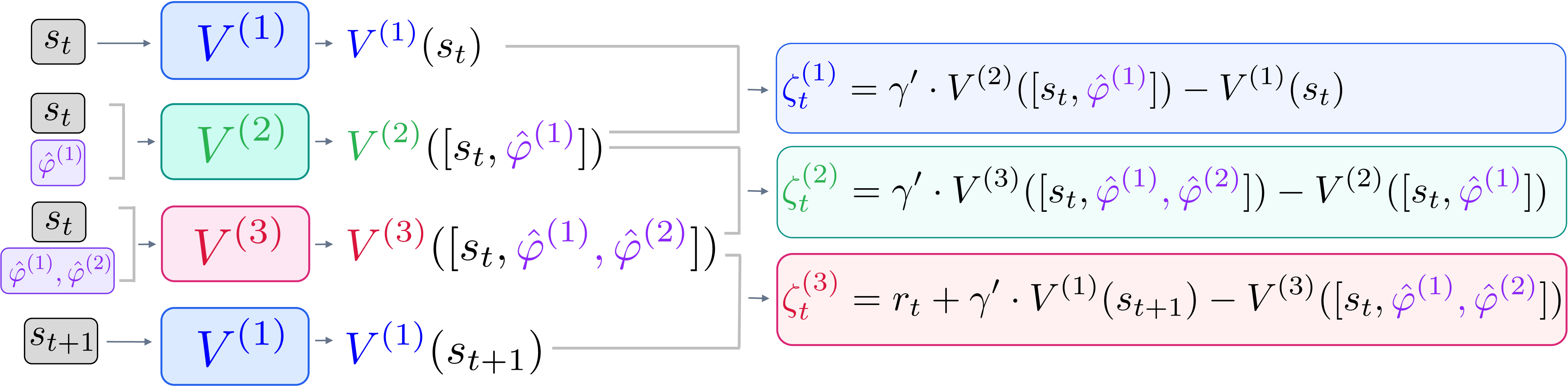
Figure 1: Value Network Architecture for the PPO instantiation of ACPO (ACPPO) with \(N=3\) agents. Each agent’s value function \(V^{(i)}\) takes the state augmented with preceding belief estimates as input. TD residuals chain across Agent 1, Agent 2, and Agent 3..
4.1.0.1 Agent-Chained TD Residuals.
Following the Bellman operators in Definition [def:bellman95operators], the Temporal Difference (TD) residuals are \[\begin{align} \zeta_t^{(i)} &=\gamma' V^{(i+1)}\left([s_{t}, b_t^{(i+1)}]\right) - V^{(i)}\left([s_t, b_t^{(i)}]\right), \quad \forall i\in\{1, \dots, N-1 \},\\ \zeta_t^{(N)} &= R\left([s_t, b_t^{(N)}], a^{(N)}_t\right) +\gamma' V^{(1)}(s_{t+1}) - V^{(N)}\left([s_t, b_t^{(N)}]\right) \\ &\approx r_t +\gamma' V^{(1)}(s_{t+1}) - V^{(N)}\left([s_t, b_t^{(N)}]\right), \end{align}\] where the reward \(R\) is zero for any agent \(i \in \{1, \dots, N-1\}\) during micro-steps (see Figure 1). For intermediate agents \(i < N\), the residual \(\zeta_t^{(i)}\) measures how agent \(i\)’s action shifts the value for the next agent in the chain. Only the last agent’s residual \(\zeta_t^{(N)}\) incorporates the environment reward and bootstraps to \(V^{(1)}\) at the next timestep.
4.1.0.2 Agent-Chained Generalized Advantage Estimation.
The advantage is an exponentially-weighted sum over the chained TD residuals, \[A_{t}^{(i)}([s_t, b^{(i)}_t], a^{(i)}_t)= \sum_{j=i}^N (\gamma' \lambda')^{j-i} \zeta^{(j)}_t + \sum_{k=1 }^\infty \sum_{j=1}^N (\gamma' \lambda')^{k N+j-i} \zeta_{t+k}^{(j)},\] with the full derivation provided in Appendix 14. The first sum aggregates TD residuals within the current timestep \(t\) from agent \(i\) through agent \(N\). The second sum extends across future timesteps, cycling through all \(N\) agents at each step.
4.1.0.3 PPO Objective
Using the advantage estimates, the PPO objective can be written as a variant of policy gradient with a clipped probability ratio:
\[\label{eq:ppo95objective} \begin{align} \mathcal{L}^{(i)}(\theta)= \mathbb{E} _{a^{(i)}_t \sim \pi_{\theta_{old}}^{(i)}(\cdot \mid s_{t}, b^{(i)}_t)}[ \min( w^{(i)}(s_{t},b^{(i)}_t, a^{(i)}_t) A_{t}^{(i)}, \text{ clip}\left( w^{(i)}(s_{t},b^{(i)}_t, a^{(i)}_t) , 1\pm\epsilon \right)A_{t}^{(i)} ) ] \end{align}\tag{3}\]
where \(w^{(i)}(s_{t},b^{(i)}_t, a^{(i)}_t):= \pi_{\theta}^{(i)}(a^{(i)}_t | s_{t}, b^{(i)}_t) / \pi_{\theta_{old}}^{(i)}(a^{(i)}_t | s_{t}, b^{(i)}_t)\).
4.1.0.4 Per-Agent Importance Sampling Ratio.
The importance sampling ratio \(w^{(i)}\) in Eq. 3 is naturally defined per agent and does not require a product over all agents’ policies. In contrast, alternating policy update approaches such as HAPPO and HATRPO use a ratio of the form \(w^{(i)}_{\text{BR}}(s, \vec{a}):= \prod_{j=1}^N\pi^{(j)}_{\theta}(a^{(j)} | s) / \prod_{j=1}^N\pi^{(j)}_{\theta_{old}}(a^{(j)} | s),\) whose variance scales exponentially with the number of agents [18]. MAPPO requires the same ratio in principle but ignores the product, resulting in a biased PPO objective.
4.2 Belief Approximation for Practical Implementations↩︎
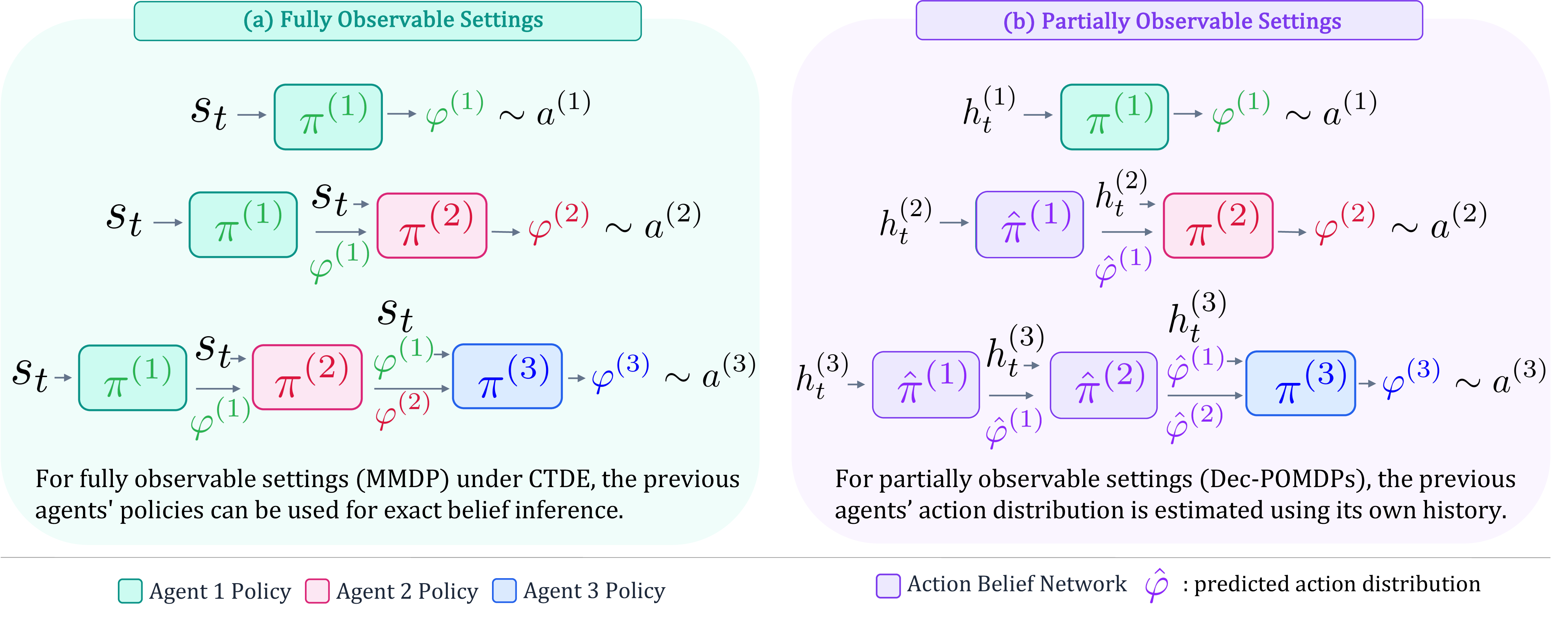
Figure 2: Policy architecture for ACPO under (a) fully observable settings (MMDP) and (b) partially observable settings (Dec-POMDP). In the MMDP case, \(\vec{\varphi}^{<i}_t\) is computed exactly by querying preceding agents’ networks with the shared state \(s_t\). In the Dec-POMDP case, each agent learns an action belief network \(\hat{\pi}^{(j)}\) to approximate \(\varphi^{(j)}_t\) from its own history..
The AC-BMDP belief \(b^{(i)}_t\) is fully determined by \(\vec{\varphi}^{<i}_t = [\varphi^{(1)}_t, \dots, \varphi^{(i-1)}_t]\), a distribution over preceding actions within each environment step. Computing \(\vec{\varphi}^{<i}_t\) therefore reduces to evaluating the preceding agents’ policy networks at the current step. The procedure differs depending on whether the environment is fully or partially observable (Figure 2).
4.2.0.1 MMDP (Fully Observable)
All agents share the same state \(s_t\), so the preceding agents’ action distributions are obtained exactly by querying their policy networks. With shared parameters and agent ID as an additional input, \(\varphi^{(j)}_t = \pi_\theta(s_t, \varphi^{(1)}_t, \dots, \varphi^{(j-1)}_t;\, j)\) for each \(j < i\). With separate parameters, agent \(i\) maintains copies of \(\pi^{(j)}_{\theta^{(j)}}\) for \(j < i\), accessible during centralized training under CTDE, and queries them directly with \(s_t\). In both cases, \(\vec{\varphi}^{<i}_t\) is computed exactly.
4.2.0.2 Dec-POMDP (Partially Observable).
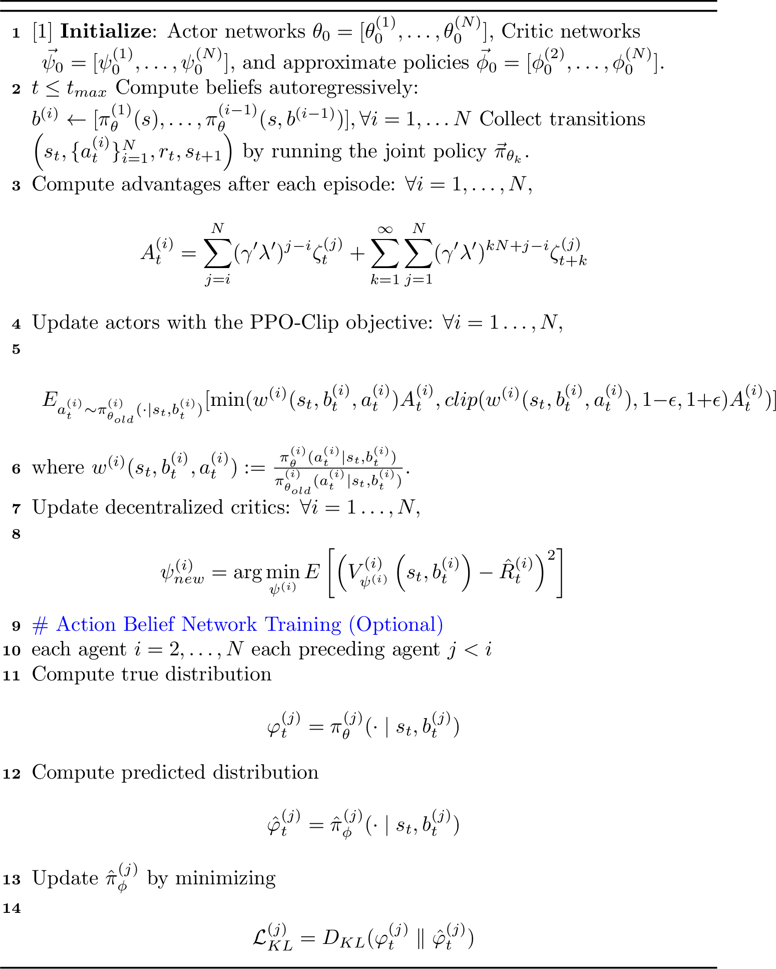
In Dec-POMDPs, each agent conditions on its own action-observation history \(h^{(i)}_t = \langle \vec{o}^{(i)}_{\leq t}, \vec{a}^{(i)}_{< t} \rangle\), and the preceding agents’ action distributions cannot be computed exactly. We apply agent modelling [25], [26] [27], where each agent maintains an action belief network \(\hat{\pi}^{(j)}\) that predicts \(\vec{\varphi}^{<i}_t\) from its own history, \[\hat{\varphi}^{(j)}_t = \hat{\pi}^{(j)}(h^{(i)}_t), \quad j < i.\] The network is trained by minimizing \(D_{KL}(\varphi^{(j)}_t \| \hat{\varphi}^{(j)}_t)\) against the centralized target \(\varphi^{(j)}_t = \pi^{(j)}(h^{(j)}_t)\), available during centralized training. Algorithm 9 in Appendix [appendix:pseudocodes] provides the full procedure.
4.2.0.3 Relation to Previous Work in Opponent Modelling
Our work is related to the concept of interactive states [28], which augments the state with a model of other agents. Such opponent models often face the problem of infinite recursive reasoning, where agent \(i\) must model agent \(j\)’s model of agent \(i\), and so on. Public belief states [29]–[31] break this recursion by introducing a common belief state shared by all agents. The AC-BMDP avoids it differently. Serialization makes the reasoning dependencies acyclic, where agent \(i\) only requires the action distributions of preceding agents \(j < i\) and never models future agents. As a result, recursive belief hierarchies do not arise.
Other Deep MARL approaches typically treat opponent modelling as an auxiliary algorithmic module. LIAM [26], for instance, augments policy inputs with a representation trained to predict the private histories of all other agents \(\vec{h}^{-i}\). Specifically, LIAM’s decoder is trained against the sampled observations and realized actions of the modelled agents as reconstruction targets. The realized actions are a higher-variance learning signal than the underlying action distribution because actions are stochastically sampled from the behavior policy. In ACPO, the action belief networks are trained directly against the action distributions of preceding agents, which is a deterministic quantity required by the chained Bellman operator.

Figure 3: Return for Multi-Robot Warehouse (RWARE) where return is the number of items collected and delivered successfully. The mean and standard error over 10 seeds are reported for all tasks. The performance advantage of ACPPO grows significantly as the number of agents increase and the map becomes smaller, where agents need higher levels of coordination being crowded in a tight space..
| VDN | QMIX | HAPPO | MAPPO | ACPPO (Ours) | |
|---|---|---|---|---|---|
| protoss_5_vs_5 | \(16.20 \pm 0.49\) | \(\mathbf{16.53 \pm 0.55}\) | \(15.93 \pm 0.54\) | \(\mathbf{17.03 \pm 0.92}\) | \(\mathbf{16.98 \pm 0.47}\) |
| zerg_5_vs_5 | \(11.77 \pm 0.41\) | \(\mathbf{14.33 \pm 0.63}\) | \(11.81 \pm 0.63\) | \(11.84 \pm 0.80\) | \(12.82 \pm 1.39\) |
| protoss_10_vs_11 | \(\mathbf{14.74 \pm 0.50}\) | \(\mathbf{14.53 \pm 1.06}\) | \(13.39 \pm 0.50\) | \(14.57 \pm 0.33\) | \(\mathbf{15.23 \pm 0.30}\) |
| terran_10_vs_11 | \(11.59 \pm 0.67\) | \(\mathbf{13.50 \pm 0.73}\) | \(10.57 \pm 0.58\) | \(12.03 \pm 0.50\) | \(\mathbf{13.98 \pm 1.43}\) |
| zerg_10_vs_11 | \(13.38 \pm 0.63\) | \(\mathbf{14.61 \pm 0.66}\) | \(10.77 \pm 0.35\) | \(12.48 \pm 0.52\) | \(\mathbf{13.52 \pm 1.18}\) |
}
\vskip-0.1in \end{table}

Figure 4: Comparison of On-Policy Algorithms on MA-MuJoCo (Gymnasium). In environment names such as Ant 2\(\times\)4, the first number denotes the number of agents, while the second number indicates the action dimension per agent..
5 Experimental Results↩︎
5.0.0.1 Environments
We focus our empirical evaluation on Multi-Robot Warehouse (RWARE) [32] which simulates a real-world warehouse environment consisting of multiple robots picking up requested shelves and returning them to a designated location. The main challenge in RWARE is coordination where the agents must avoid collisions and maximize the number of shelves successfully delivered. We also evaluate our approach on StarCraft Multi-Agent Challenge v2 (SMACv2) [33] and Multi-Agent MuJoCo [34], which are popular benchmarks in cooperative MARL with discrete and continuous action spaces, respectively. For SMACv2 and MA-MuJoCo, we closely follow the experimental setup in [15].
5.0.0.2 Baselines
Our main baselines for ACPPO are MAPPO, representing independent policy optimization, and HAPPO/HATRPO, representing alternating policy optimization5. MAPPO and HAPPO are the current state-of-the-art on-policy methods in the three domains we consider. Following the baselines considered in [15], we also compare against value decomposition methods including VDN [16] and QMIX [17], which are off-policy value-based methods for discrete action spaces which shows strong performance in SMACv2.
For a fair comparison, we use the code for all baselines provided in MARLLib [35], with the same PPO backbone. For all baselines, we use the reported hyperparameters from [32] for RWARE, from [33] for SMACv2 and from [15] for MA-MuJoCo. We only tune appropriate values when the code failed to reproduce the reported performance. For MAPPO, we found the reported hyperparameters to be sufficient for reproducing the results. For ACPPO, the same hyperparameters as MAPPO are used for all experiments in order to isolate the effect of agent-chaining, and do not conduct any additional hyperparameter tuning specific to ACPPO. Furthermore, we set the total number of parameters used by the policy to be similar between ACPPO (policy + action belief network) and the baselines (policy). Further details on the policy network as well as hyperparameters are provided in Appendix 20.
5.0.0.3 Comparative Evaluation
Our main results in Figure 3 show that ACPPO outperforms all baselines6 on all tasks in RWARE, despite having the same PPO backbone and the same hyperparameters as MAPPO. We also see that the gap widens substantially as the number of agents increases, where the widest gap is seen in 8-agent and 12-agent domains. This provides evidence that ACPPO performs substantially better when the environment requires higher levels of coordination. Intuitively, the 12-agent maps require the most coordination among agents since it is the scenario with the most agents crowded in a tight space. Thus, the performance gap jumps even further for the tiny map.
In the results for MA-MuJoCo (Figures 4) and SMACv2 (Table ¿tbl:table:smacv295results?), ACPPO is on par with or outperforms all baselines on all tasks. Crucially, ACPPO outperforms or matches MAPPO on all tasks with the same hyperparameters, which demonstrates the benefit of agent-chaining. For SMACv2, ACPPO outperforms all on-policy baselines, MAPPO and HAPPO. ACPPO is also the only on-policy algorithm competitive with QMIX.
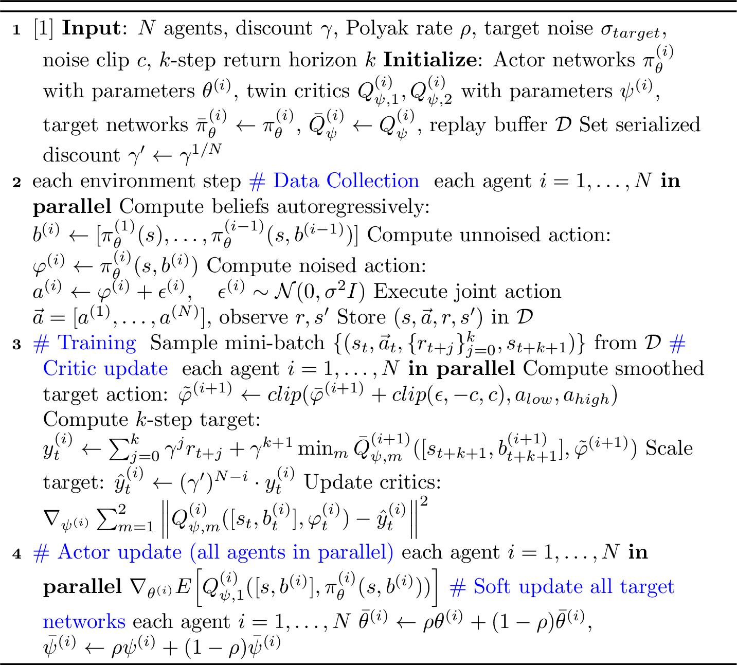
Finally, we also provide additional experimental results in Appendix 18 for an off-policy instantiation of ACPO called ACTD3, which incorporates agent-chaining into TD3 [20]. The algorithm is described in Appendix 16. The performance of ACTD3 is compared against strong off-policy baselines for continuous control, including MADDPG [11] a simultaneous policy optimization method and HATD3 [15] an alternating policy optimization method. The results for MA-MuJoCo (Figure 12) show that ACTD3 consistently outperforms all baseline methods, and shows that agent-chaining can be generally applied to off-policy algorithms as well.
5.0.0.4 Ablation Results
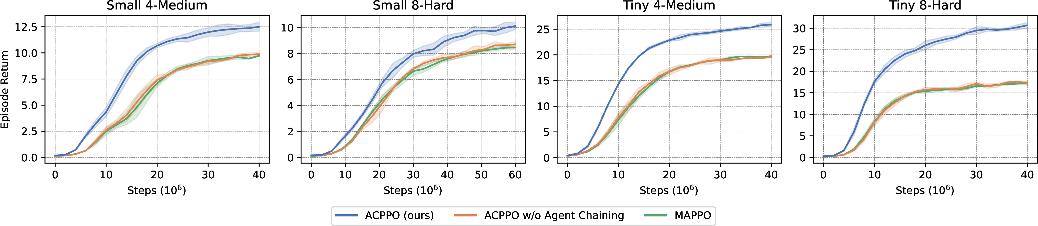
We ablate the core component of ACPPO, which is the advantage computation based on agent chaining. As shown in Figure 5, the variant ACPPO without agent chaining can be interpreted as MAPPO augmented with belief states as additional policy inputs. The performance of this variant remains close to MAPPO, indicating that the observed gains of ACPPO are not attributable to the extra input, but rather to the agent-chained advantage computation itself.
6 Conclusion↩︎
We introduced an exact decomposition of the cooperative MMDP policy gradient into a sum of per-agent terms, each computable from a per-agent score function and a decentralized critic, with no structural assumption on the joint value function. The decomposition is enabled by the Agent-Chained Belief MDP, which lifts the simultaneous joint decision into a serialized one where each agent conditions on a belief over the actions of preceding agents. We instantiated this as ACPO with on-policy and off-policy variants, and showed empirically that it outperforms strong baselines on Multi-Robot Warehouse, SMACv2, and MA-MuJoCo, with the gap widening as the number of agents grows.
6.0.0.1 Limitations and Future Work
First, the belief computation scales linearly with the number of agents. Each agent \(i\) requires \(i-1\) forward passes to compute \(\vec{\varphi}^{<i}\), and the last agent effectively requires \(N-1\) sequential forward passes. Hence the total number of forward passes across all agents grows as \(\mathcal{O}(N^2)\). While the wall-clock overhead remains modest in our experiments (Appendix 19), this scaling could become a bottleneck for domains with very large numbers of agents. A promising avenue for future work is to distill the autoregressive belief computation into a single feedforward network, where each agent directly predicts \(\vec{\varphi}^{<i}\) from the state (or observation history) without sequential queries. Second, our work follows the standard MMDP setup in CTDE, so our decomposition relies on full observability. The correct form of the policy gradient for Dec-POMDPs under CTDE remains open: existing theorems are established under centralized control via occupancy states [36], while practical CTDE methods rely on surrogates such as state-based centralized critics that are known to be biased under partial observability [37]. A proper treatment of the agent-chained decomposition under partial observability would require analysis through occupancy states or public beliefs [30], [31], which we leave to future work.
7 Limitations of Previous Methods↩︎
| A | B | |
|---|---|---|
| A | 0 | 1 |
| B | 1 | 2 |
7.0.0.1 Decomposable Matrix Games
In this matrix game, the rewards can be additively decomposed. The individual utility functions can be decomposed as follows: \(r^{(1)}(A)=r^{(2)}(A)=0\) and \(r^{(1)}(B)=r^{(2)}(B)=1\).
As described in Section 2.2, independent policy optimization methods such as MAPPO optimize \[A^{(i)}(s, a^{(i)}) := \mathbb{E}_{\pi^{(i)}, \vec{\pi}^{-i}} \left[ A\bigl(s, a^{(i)}, \vec{a}^{-i}\bigr) \right]\] for each agent separately, treating \(\vec{\pi}^{-i}\) as fixed at the current policy.
Suppose the joint policy is initialized at the suboptimal outcome \(AA\), which yields reward \(0\). For agent 1, deviating to \(B\) while agent 2 keeps playing \(A\) leads to \(R(BA) = 1 > R(AA) = 0\), so its independent update pushes probability mass toward \(B\). By symmetry, agent 2 also prefers deviating from \(A\) to \(B\), since \(R(AB) = 1 > R(AA) = 0\). When both agents update simultaneously, the joint policy moves toward \(BB\), which attains the global optimum with reward \(2\). In this decomposable setting, each agent’s local improvement direction is aligned with improvement of the joint policy.
| A | B | |
|---|---|---|
| A | 0 | 1 |
| B | 1 | -10 |
7.0.0.2 Matrix Game motivating alternating policy optimization
Now consider the matrix game in Table 2, and suppose the joint policy is initialized to select \(AA\), yielding a reward of \(0\). For agent 1, deviating to \(B\) while agent 2 plays \(A\) (i.e., the joint action \(BA\)) gives a higher reward than \(AA\), so its independent update drives it toward playing \(B\). The same holds symmetrically for agent 2, since \(AB\) yields a higher reward than \(AA\). Because both agents update independently and simultaneously, the joint policy can move toward \(BB\), which receives a reward of \(-10\). Note that further updates will move the joint policy toward AA again. In other words, independent policy optimization methods will not converge.
This failure mode motivates alternating policy optimization methods such as HAPPO, where each agent updates its policy while holding the other agents fixed, and guarantee monotonic improvement of the joint policy at each update step. In the game in Table 2, if agent 1 updates first, it will switch to playing \(B\) deterministically, since \(BA\) is better than \(AA\). When agent 2 subsequently updates, it prefers to keep playing \(A\), because \(BA\) is better than \(BB\). Thus the joint policy converges to \(BA\), avoiding the catastrophic outcome \(BB\). However, as discussed in detail in Section 2.3, the fixed points of alternating policy optimization methods are Nash Equilibria, which is not necessarily the optimal joint policy. In the game in Table 6, all the Nash Equilibria happen to be globally optimal, whereas this is not the case for the matrix game in Table ¿tbl:matrix95game95policy95values95main95text?. In contrast, ACPI directly targets the optimal joint policy in the underlying MMDP and therefore does not rely on value decomposition assumptions or on properties of Nash equilibria.
8 Details on Centralized Training with Decentralized Execution (CTDE)↩︎
In our work, we consider the standard MARL paradigm of Centralized Training Decentralized Execution (CTDE), which allows multiple policies to be jointly trained but must be executed in a decentralized fashion.
Here we introduce related work in three different settings that are often considered in MARL: Centralized Training Centralized Execution (CTCE), Centralized Teacher with Decentralized Student (CTDS) 7, and CTDE.
8.0.0.1 Centralized Training Centralized Execution (CTCE)
Centralized Training Centralized Execution (CTCE) methods such as Multi-Agent Transformer (MAT) [39] use a joint policy of the form \(\pi(a^{(1)}, \dots ,a^{(N)}|s)\) during both training rollouts and execution. MAT is a centralized Transformer model defined on the joint action space, and uses a joint observation encoder and joint policies during both training and execution. While a decentralized policy version is also considered, MAT requires a joint observation encoder during both training and execution. In MMDPs, the CTCE setting reduces to a Factored-Action MDP [40], [41], which is a single-agent MDP with factored action spaces. In this case, single-agent techniques such as policy iteration and value iteration can be applied directly.
Generally, centralized control (CTCE) is not applicable to many real-world multi-agent systems such as power grids [4], traffic signal control [2], and large-scale fleet management [3] due to the large joint action space and prohibitive communication costs.
8.0.0.2 Centralized Teacher with Decentralized Student (CTDS)
[42]–[44] aims to decentralize centralized solutions, by assuming that a single-agent joint policy can be used for training rollout. This joint policy is used during centralized training and distilled to decentralized policies before execution. As a single-agent problem, this assumption makes convergence to optimal policies straightforward as in the CTCE case. We can view this setting as a special case of our work where we assume further access to a joint policy during training rollouts. With this additional assumption, we can solve the serialized problem introduced in Appendix 10 without considering beliefs. However, this line of research inherits similar weaknesses of CTCE, and cannot be applied to many real-world multi-agent systems with a massive action space or prohibitive communication costs.
8.0.0.3 Centralized Training Decentralized Execution (CTDE)
In CTDE, the policy must be decentralized (fully factorized) during both training and execution, with the policy form \(\vec{\pi} = \langle \pi^{(1)}, \dots \pi^{(N)} \rangle\) where \(\pi^{(i)}: S\rightarrow A^{(i)}\). This is the natural MARL paradigm we consider in our work. Algorithms for independent policy optimization methods [11], [13], alternating policy optimization methods [14], [15], [23] as well as value decomposition methods [17], [19] all fall under CTDE.
9 Exact Calculation of Policies in the Matrix Game↩︎
None
Figure 6: 3x3 Matrix Game.
Here we provide details on how ACPI (the tabular version of ACPO) can solve the Matrix Game provided in Table ¿tbl:matrix95game95policy95values95main95text? and repeated in Figure 6.
Due to serialization, ACPO considers this as a 2-step game even though the underlying game is a 1-step game. Since we are in a simple toy setting which can be solved by policy iteration, we only consider deterministic action distributions \(\varphi\).
Policy evaluation for agent 1 is conducted as follows. \[\begin{align} &Q^{(1)}(\varphi^{(1)}) = \gamma'\mathbb{E}_{\substack{b^{(2)}=\varphi^{(1)} \\ \varphi^{(2)} \sim \pi^{(2)}(\cdot \mid b^{(2)})}} \left[Q^{(2)}(b^{(2)}, \varphi^{(2)}) \right] \end{align}\] When we only consider deterministic \(\varphi\): \[\begin{align} &Q^{(1)}(\delta^{(1)}_A) = \gamma'\mathbb{E}_{\substack{a^{(2)} \sim \pi^{(2)}(\cdot \mid b^{(2)}=A)}} \left[Q^{(2)}(b^{(2)}=A, a^{(2)}) \right] \\ &Q^{(1)}(\delta^{(1)}_B) = \gamma'\mathbb{E}_{\substack{a^{(2)} \sim \pi^{(2)}(\cdot \mid b^{(2)}=B)}} \left[Q^{(2)}(b^{(2)}=B, a^{(2)}) \right] \\ &Q^{(1)}(\delta^{(1)}_C) = \gamma'\mathbb{E}_{\substack{a^{(2)} \sim \pi^{(2)}(\cdot \mid b^{(2)}=C)}} \left[Q^{(2)}(b^{(2)}=C, a^{(2)}) \right] \\ \end{align}\] where we have used \(b^{(2)} =A\) to denote the fact that agent 2 knows with probability 1 that it is in state \(A\) since it knows that \(\pi^{(1)}\) chooses \(A\) deterministically. Also, we used the notation \(\delta^{(1)}_A\) to denote a particular action distribution \(\varphi\) which deterministically selects \(A\).
For agent 2, policy evaluation is simply the reward function given in the Matrix game: \[\begin{align} &Q^{(2)}(b^{(2)}=A, A)=R(A, A) = 5\\ &\qquad \qquad \vdots\\ &Q^{(2)}(b^{(2)}=B, B)=R(B, B) = 10\\ &\qquad \qquad \vdots\\ &Q^{(2)}(b^{(2)}=C, C)=R(C, C) = 20\\ \end{align}\]
For policy improvement, \[\begin{align} &\pi^{(2)}(b^{(2)}=A) \leftarrow \arg \max_{a^{(2)} \in \{A, B, C \}}Q^{(2)}(b^{(2)}=A, a^{(2)}) \\ &\pi^{(2)}(b^{(2)}=B) \leftarrow \arg \max_{a^{(2)} \in \{A, B, C \}}Q^{(2)}(b^{(2)}=B, a^{(2)}) \\ &\pi^{(2)}(b^{(2)}=C) \leftarrow \arg \max_{a^{(2)} \in \{A, B, C \}}Q^{(2)}(b^{(2)}=C, a^{(2)})\\ \end{align}\].
Thus, \(\pi^{(2)}\) will select \(A, B, C\) given agent 1 deterministically selects \(A, B, C\), respectively.
For agent 1, \[\begin{align} &\pi^{(1)} \leftarrow \arg \max_{a^{(1)} \in \{A, B, C \}}\gamma'Q^{(2)}(b^{(2)}=a^{(1)}, \pi^{(2)}(b^{(2)}=a^{(1)})) \\ \end{align}\]
Now, let’s say we are in an adversarial starting point where the policy is initialized to deterministically select \((A, A)\).
Initially, policy improvement for \(\pi^{(1)}\) leads agent 1 to continue selecting \(A\) since \(\pi^{(2)}\) deterministically selects A and \(R(A, A)=5\) is better than \(R(B, A)=R(C,A)=-20\). However, after the first iteration, agent 2 will update its policy to select \(A, B, C\) for \(b^{(2)}=A, b^{(2)}=B, b^{(2)}=C\), respectively. Thus, agent 1 in iteration 2 will select \(C\) since \(C = \arg \max_{a^{(1)}} \gamma' Q^{(2)}(b^{(2)}=a^{(1)}, \pi^{(2)})\), where \(\pi^{(2)}\) is now updated.
10 Serializing the MMDP↩︎
The serialized multi-agent problem can be described as follows:
Action space \(\mathcal{A}^{(i)}\) of individual actions for some \(i \in \mathcal{N}\)
States \([s_{t}, \vec{a}_{t}^{<i}]\) which augments the original state space with actions selected by previous agents \(\vec{a}_{t}^{<i}\).
Reward function \[R([s_{t}, \vec{a}_{t}^{<i}], a_{t}^{(i)})= \begin{cases} R(s_t, \vec{a}_{t}) &\text{ if } i=N\\ 0 &\text{ otherwise }\\ \end{cases}\]
Transition function \[\begin{align} &T([s_{t+1}, \emptyset]\mid [s_{t}, \vec{a}_{t}^{<i}], a_{t}^{(i)})= T(s_{t+1} \mid s_t, \vec{a}_{t}) \text{ if } i=N\\ &T([s_{t}, \vec{a}_{t}^{<i+1}]\mid [s_{t}, \vec{a}_{t}^{<i}], a_{t}^{(i)}) \\ &\qquad = \mathbb{I}\{ [\vec{a}_{t}^{<i}, a_t^{(i)}]= \vec{a}_{t}^{<i+1}\}\text{ if } i\in \{1, \dots, N -1\} \\ \end{align}\]
Discount factor \(\gamma'\) where \(\gamma'=\gamma^{1/N}\)
The optimal policy for this serialized problem is in fact optimal for the original MMDP as well.
theoremThmSerializationEquivalence[36] For every MMDP, there exists a serialized multi-agent problem, of which its optimal policy is also optimal for the underlying MMDP.
Proof. Let \(\vec{\pi} = \langle {\pi}^{(1)}, \dots, {\pi}^{(N)}\rangle\) be any policy over the serialized MMDP. \[\begin{align} &V^{(i)}([s, \vec{a}^{<i}]; \vec{\pi}) \\ &= \mathbb{E}\left[\sum_{j=i}^N (\gamma')^{j-i} R\left(s_{0}, \vec{a}^{<j}_0, a^{(j)}_0 \right) \mid s_0 = s, \vec{a}_0^{<i} = \vec{a}^{<i}, \vec{\pi}\right] +\mathbb{E}\left[\sum_{t=1} \sum_{j=1}^N (\gamma')^{tN+j-i} R\left(s_{t}, \vec{a}^{<j}_t, a^{(j)}_t \right) \mid \vec{\pi}\right] \\ &= \mathbb{E}\left[ (\gamma')^{N-i} R\left(s_{0}, \vec{a}^{<N}_0, a^{(N)}_0 \right) \mid s_0 = s, \vec{a}_0^{<i} = \vec{a}^{<i}, \vec{\pi}\right] +\mathbb{E}\left[\sum_{t=1} (\gamma')^{tN+N-i} R\left(s_{t}, \vec{a}^{<N}_t, a^{(N)}_t \right) \mid \vec{\pi}\right] \\ &= \mathbb{E}\left[ (\gamma')^{N-i}R\left(s_{0}, \vec{a}^{<N}_0, a^{(N)}_0 \right) \mid s_0 = s, \vec{a}_0^{<i} = \vec{a}^{<i}, \vec{\pi}\right] +\mathbb{E}\left[\sum_{t=1} (\gamma')^{N-i} \gamma^t R\left(s_{t}, \vec{a}^{<N}_t, a^{(N)}_t \right) \mid \vec{\pi}\right] \\ &= \mathbb{E}\left[\sum_{t=0} (\gamma')^{N-i} \gamma^t R\left(s_{t}, \vec{a}^{<N}_t, a^{(N)}_t \right) \mid s_0 = s, \vec{a}_0^{<i} = \vec{a}^{<i},\vec{\pi}\right] \\ &= (\gamma')^{N-i}\mathbb{E}\left[\sum_{t=0} \gamma^t R\left(s_{t}, \vec{a}^{<N}_t, a^{(N)}_t \right) \mid s_0 = s, \vec{a}_0^{<i} = \vec{a}^{<i}, \vec{\pi}\right] \\ \end{align}\]
\(V^{(1)}(s) =(\gamma')^{N-1} \mathbb{E}\left[\sum_{t=0} \gamma^t R\left(s_{t}, \vec{a}^{<N}_t, a^{(N)}_t \right) \mid s_0=s, \vec{\pi}\right]\) for agent \(1\).
\(V^{(N)}([s, \vec{a}^{<N}]) = \mathbb{E}\left[\sum_{t=0} \gamma^t R\left(s_{t}, \vec{a}^{<N}_t, a^{(N)}_t \right) \mid s_0 = s, \vec{a}_0^{<N} = \vec{a}^{<N}, \vec{\pi}\right]\) for agent \(N\).
Thus, we have established that any policy \(\vec{\pi}\) in the serialized problem will obtain the same expected value in the MMDP (times a constant factor). There is a 1-1 mapping between serialized and simultaneous policies which yield the same value. ◻
11 Belief Update↩︎
\[\begin{align} \tau&\left([s_{t},b_{t}^{(i)}],\varphi_t^{(i)}\right)(\vec{a}_{t}^{<i+1})\\&=\frac{1}{\eta([s_{t},b_{t}^{(i)}],\varphi_t^{(i)})}\sum_{\vec{a}_{t}^{<i}}b_{t}^{(i)}( \vec{a}_{t}^{<i}) T\left([s_{t},\vec{a}_{t}^{<i+1}]|[s_t,\vec{a}_{t}^{<i}],\varphi_t^{(i)}\right) \\ &=\frac{1}{\eta([s_{t},b_{t}^{(i)}],\varphi_t^{(i)})}\sum_{\vec{a}_{t}^{<i}}b_{t}^{(i)}( \vec{a}_{t}^{<i}) \sum_{a_t^{(i)}} \varphi_t^{(i)}(a_t^{(i)}) T\left([s_{t},\vec{a}_{t}^{<i+1}]|[s_t,\vec{a}_{t}^{<i}],a_{t}^{(i)}\right) \\ \end{align}\] Finally, \(\eta\) is the normalization factor defined as \[\begin{align} &\eta([s_{t},b_{t}^{(i)}],\varphi_t^{(i)})=\sum_{\vec{a}_{t}^{<i+1}}\sum_{\vec{a}_{t}^{<i}}b_{t}^{(i)}( \vec{a}_{t}^{<i}) \sum_{a_t^{(i)}} \varphi_t^{(i)}(a_t^{(i)}) T\left([s_{t},\vec{a}_{t}^{<i+1}]|[s_t,\vec{a}_{t}^{<i}],a_{t}^{(i)}\right) \end{align}\]
12 Proofs for Policy Iteration Convergence↩︎
Here we present Agent-Chained Policy Iteration (ACPI), a policy iteration procedure defined on the AC-BMDP. ACPI is the tabular version of ACPO introduced in Section 4. Unlike alternating policy optimization approaches [15] where the fixed point of policy iteration is a NE, we prove that ACPI converges to the optimal joint policy of the MMDP.
12.1 Agent-Chained Policy Evaluation↩︎
By repeatedly applying \(\mathcal{T}^{\vec{\pi}}\), we can obtain the \(Q\)-values for a given joint policy \(\vec{\pi}\):
lemmaLemmaPolicyEvaluation (Agent-Chained Policy Evaluation) The Agent-Chained Bellman Operators in Definition [def:bellman95operators] are a contraction mapping under the infinity norm. Thus, starting with any \(\vec{Q}=\langle Q^{(1)}, \dots Q^{(N)}\rangle\) and a joint policy \(\vec{\pi}=\langle \pi^{(1)}, \dots, \pi^{(N)}\rangle\), the repeated application of \(\mathcal{T}^{\vec{\pi}}\) will return a set of Q-values for each agent \(\langle Q^{(1, \vec{\pi})}, \dots Q^{(N, \vec{\pi})}\rangle\) in the limit.
Proof. First, note that we can view \(\langle Q^{(1)}, \dots, Q^{(N)}\rangle\) as a single Q-function with the state space further augmented by agent ID. Under this perspective, we now have a single policy denoted as \(\pi\) and a corresponding value function \(Q^{\pi}\), defined on the AC-BMDP.
Since the AC-BMDP is a single-agent Belief MDP, the rest follows standard convergence results of policy evaluation [45], which we include for completeness.
For any agent \(i \in \{1, \dots N-1 \}\), state \([s, b^{(i)}, i]\), action \(\varphi^{(i)}\) and arbitrary Q-values \(Q_1, Q_2\), \[\begin{align} &\left|\mathcal{T}^{\pi}Q_1([s, b^{(i)}, i], \varphi^{(i)} ) - \mathcal{T}^{\pi}Q_2([s, b^{(i)}, i], \varphi^{(i)} )\right| \\ & = \left|\mathbb{E}_{\substack{[s, b^{(i+1)}, i+1] = T([s, b^{(i)}, i], \varphi^{(i)})\\\varphi^{(i+1) } \sim \pi(\cdot \mid s, b^{(i+1)}, i+1)}} \left[\gamma'Q_1([s, b^{(i+1)}, i+1], \varphi^{(i+1)} ) - \gamma'Q_2([s, b^{(i+1)}, i+1], \varphi^{(i+1)} )\right] \right| \\ & \leq \gamma'\max_{\varphi^{(i+1)} }\left|Q_1([s, b^{(i+1)}, i+1], \varphi^{(i+1)} ) - Q_2([s, b^{(i+1)}, i+1], \varphi^{(i+1)} )\right| \\ & \leq \gamma'\max_{\varphi^{(i+1)}, b^{(i+1)}, j \in \{1, \dots, N\} }\left|Q_1([s, b^{(i+1)}, j], \varphi^{(i+1)} ) - Q_2([s, b^{(i+1)}, j], \varphi^{(i+1)} )\right| \\ \end{align}\]
For agent \(N\), \[\begin{align} &\left|\mathcal{T}^{\pi}Q_1([s, b^{(N)}, N], \varphi^{(N)} ) - \mathcal{T}^{\pi}Q_2([s, b^{(N)}, N], \varphi^{(N)} )\right| \\ & = \left|\mathbb{E}_{\substack{[s', 1] \sim T(\cdot \mid [s, b^{(N)}, N], \varphi^{(N)})\\\varphi^{(1) } \sim \pi(\cdot \mid s', 1)}} \left[\gamma'Q_1([s', 1], \varphi^{(1)} ) - \gamma'Q_2([s', 1], \varphi^{(1)} )\right] \right| \\ & \leq \gamma'\max_{s', \varphi^{(1)} }\left|Q_1([s', 1], \varphi^{(1)} ) - Q_2([s', 1], \varphi^{(1)} )\right| \\ & \leq \gamma'\max_{s', \varphi^{(1)}, j \in \{1, \dots, N\} }\left|Q_1([s', j], \varphi^{(1)} ) - Q_2([s', j], \varphi^{(1)} )\right| \\ \end{align}\]
Thus, \(\mathcal{T}^\pi\) is a contraction mapping under the infinity norm, i.e. there exists \(\gamma' \in [0, 1)\) such that
\[\| \mathcal{T}^{\pi}Q_{1} - \mathcal{T}^{\pi}Q_2\|_\infty \leq \gamma' \| Q_{1} - Q_2\|_\infty\]
Since \(\mathcal{T}^{\pi}\) is a contraction mapping, we have the following: \[\begin{align} \| Q_k - Q^\pi\|_\infty &= \| \mathcal{T}^{\pi}Q_{k-1} - \mathcal{T}^{\pi}Q^\pi\|_\infty \\ & \leq \gamma' \| Q_{k-1} - Q^\pi\|_\infty\\ & \;\;\vdots\\ & \leq ({\gamma'})^k \| Q_{0} - Q^\pi\|_\infty\\ \end{align}\] If we let \(k \rightarrow \infty , \| Q_k - Q^\pi\|_\infty =0\), and \(\lim_{k\rightarrow \infty}Q_k = Q^\pi\). By the Banach fixed-point theorem, this solution is unique. ◻
12.2 Agent-Chained Policy Improvement↩︎
During policy improvement, each agent’s policy \(\pi^{(i)}\) is updated to select the greedy action distribution with respect to its own \(Q^{(i)}\): \[\label{eq:policy95improvement} \begin{align} \pi^{(i)}_{new}([s, b^{(i)}]) \leftarrow \arg \max_{\varphi^{(i)}} Q^{(i,\vec{\pi})}([s, b^{(i)}], \varphi^{(i)}) \qquad \forall i, b^{(i)}, s . \end{align}\tag{4}\]
lemmaLemmaPolicyImprovement (Agent-Chained Policy Improvement) Given a policy \(\vec{\pi}=\langle \pi^{(1)}, \dots, \pi^{(N)}\rangle\), let \(Q^{(i,\vec{\pi})}\) denote the \(i\)-th agent’s value function for a joint policy \(\vec{\pi}\). If we update the new policy \(\vec{\pi}_{new}=\langle \pi^{(1)}_{new}, \dots, \pi^{(N))}_{new}\rangle\) by Eq. 4 , then \[Q^{(i, \vec{\pi}_{new})} ([s, b^{(i)}], \varphi^{(i)})\geq Q^{(i, \vec{\pi})} ([s, b^{(i)}], \varphi^{(i)})\]
Proof. As in the proof for Lemma [lemma:policy95evaluation], we consider \(\vec{\pi}\) to be a single policy \(\pi\) which is augmented by agent ID in the state space.
For any \(i \in \{1, \dots N-1 \}, s, b^{(i)}, \varphi^{(i)}\), \[\begin{align} Q^{{\pi}}([s, b^{(i)}, i], \varphi^{(i)}) &= \gamma' \mathbb{E}_{\substack{[s, b^{(i+1)}, i+1]= T([s, b^{(i)}, i], \varphi^{(i)}) \\ \varphi^{(i+1)} \sim \pi(\cdot \mid [s, b^{(i+1)}, i+1])}}\left[Q^{{\pi}}\left([s, b^{(i+1)}, i+1], \varphi^{(i+1)}\right) \right] \\ & \leq \gamma' \mathbb{E}_{\substack{[s, b^{(i+1)}, i+1]= T([s, b^{(i)}, i], \varphi^{(i)})}}\left[\max_{\varphi^{(i+1)}}Q^{{\pi}}\left([s, b^{(i+1)}, i+1], \varphi^{(i+1)}\right) \right] \\ & = \gamma' \mathbb{E}_{\substack{[s, b^{(i+1)}, i+1]= T([s, b^{(i)}, i], \varphi^{(i)}) \\ \varphi^{(i+1)} \sim \pi_{new}(\cdot \mid [s, b^{(i+1)}, i+1])}}\left[Q^{{\pi}}\left([s, b^{(i+1)}, i+1], \varphi^{(i+1)}\right) \right] \end{align}\]
For \(i=N\) and any \(s, b^{(i)}, \varphi^{(i)}\), \[\begin{align} Q^{{\pi}}&([s, b^{(N)}, N], \varphi^{(N)})\\ &= R([s, b^{(N)}, N], \varphi^{(N)})+\gamma' \mathbb{E}_{\substack{[s', 1]= T([s, b^{(N)}, N], \varphi^{(N)}) \\ \varphi^{(1)} \sim \pi(\cdot \mid [s', 1])}}\left[Q^{{\pi}}\left([s',1], \varphi^{(1)}\right) \right] \\ & \leq R([s, b^{(N)}, N], \varphi^{(N)})+ \gamma' \mathbb{E}_{\substack{[s', 1]= T([s, b^{(N)}, N], \varphi^{(N)}))}}\left[\max_{\varphi^{(1)}}Q^{{\pi}}\left([s',1], \varphi^{(1)}\right) \right] \\ & = R([s, b^{(N)}, N], \varphi^{(N)})+ \gamma' \mathbb{E}_{\substack{[s', 1]= T([s, b^{(N)}, N], \varphi^{(N)}) \\ \varphi^{(1)} \sim \pi_{new}(\cdot \mid [s', 1])}}\left[Q^{{\pi}}\left([s',1], \varphi^{(1)}\right) \right] \\ \end{align}\] Thus, for any \(i \in \{1, \dots N \}, s, b^{(i)}, \varphi^{(i)}\), \[\begin{align} Q^{{\pi}}([s, b^{(i)}, i], \varphi^{(i)}) &\leq R([s, b^{(i)}, i], \varphi^{(i)})\\&\qquad+\gamma' \mathbb{E}_{\substack{[s, b^{(i+1)}, i+1]= T([s, b^{(i)}, i], \varphi^{(i)}) \\ \varphi^{(i+1)} \sim \pi_{new}(\cdot \mid [s, b^{(i+1)}, i+1])}}\left[Q^{{\pi}}\left([s, b^{(i+1)}, i+1], \varphi^{(i+1)}\right) \right] \\ &\;\;\vdots \\ &\leq Q^{{\pi_{new}}}([s, b^{(i)}, i], \varphi^{(i)}) \end{align}\] ◻
Crucially, since each agent’s improvement in Eq. 4 only depends on its own \(Q^{(i, \vec{\pi})}\), all agents can update their policies independently. This is unlike MA-PI [15], which requires alternating updates where \(\pi^{(i)}\) can only be improved after \(\vec{\pi}^{<i}\) has been updated.
12.3 Characterization of \(Q^{(i, *)}\)↩︎
Here we provide a useful property of the optimal Q-values of the AC-BMDP, which has an affine structure.
theoremTheoremConvexityOfQ Let \(Q^{(i, *)}\) denote the \(i\)-th agent’s Q-values for the optimal policy under an AC-BMDP. Then, \(Q^{(i, *)}\) is an affine function of \(\varphi^{(i)}\). i.e. for all \(i\in \{1, \dots, N\}, s, b^{(i)}, \varphi^{(i)}\), \[Q^{(i, *)}([s, b^{(i)}], \varphi^{(i)})=\sum_{a^{(i)}}\varphi^{(i)}(a^{(i)})Q^{(i, *)}([s, b^{(i)}], \delta_{a^{(i)}})\] where \(\delta_{a^{(i)}}\) denotes a particular action distribution which deterministically selects \(a^{(i)}\).
Proof. We prove the claim by induction.
For any \(s, {b}^{(N)}, \varphi^{(N)}\) at terminal timesteps, \[\begin{align} Q^{(N)}([s, b^{(N)}], \delta_{a^{(N)}}) &= R([s, b^{(N)}], a^{(N)}) \\ \end{align}\]
\[\begin{align} Q^{(N)}([s, b^{(N)}], \varphi^{(N)}) &= R([s, b^{(N)}], \varphi^{(N)})\\ &= \sum_{a^{(N)}}\varphi^{(N)}(a^{(N)})R([s, b^{(N)}], a^{(N)})\\ &= \sum_{a^{(N)}}\varphi^{(N)}(a^{(N)})Q^{(N)}([s, b^{(N)}], \delta_{a^{(N)}})\\ \end{align}\]
\[\begin{align} Q^{(N)}([s, b^{(N)}=\vec{a}^{<N}], \varphi^{(N)}) &= R([s, \vec{a}^{<N}], \varphi^{(N)}) \\ \end{align}\]
\[\begin{align} Q^{(N)}([s, b^{(N)}], \varphi^{(N)}) &= R([s, b^{(N)}], \varphi^{(N)})\\ &= \sum_{\vec{a}^{<N}}b^{(N)}(\vec{a}^{<N})R([s, \vec{a}^{<N}], \varphi^{(N)})\\ &= \sum_{\vec{a}^{<N}}b^{(N)}(\vec{a}^{<N})Q^{(N)}([s,\vec{a}^{<N}], \varphi^{(N)})\\ \end{align}\]
where \(\vec{a}^{<N}\) in \(Q^{(N)}([s,\vec{a}^{<N}], \varphi^{(N)})\) denotes the belief that assigns probability 1 to \(\vec{a}^{<N}\).
For agents \(i \in \{1, \dots, N-1 \}\), we recall the following definition of the belief update rule and the normalization factor: \[\begin{align} \tau\left([s_{t},b_{t}^{(i)}],\varphi_t^{(i)}\right)(\vec{a}_{t}^{<i+1})&=\frac{1}{\eta([s_{t},b_{t}^{(i)}],\varphi_t^{(i)})}\sum_{\vec{a}_{t}^{<i}}b_{t}^{(i)}( \vec{a}_{t}^{<i}) T\left([s_{t},\vec{a}_{t}^{<i+1}]|[s_t,\vec{a}_{t}^{<i}],\varphi_t^{(i)}\right) \\ &=\frac{1}{\eta([s_{t},b_{t}^{(i)}],\varphi_t^{(i)})}\sum_{\vec{a}_{t}^{<i}}b_{t}^{(i)}( \vec{a}_{t}^{<i}) \sum_{a_t^{(i)}} \varphi_t^{(i)}(a_t^{(i)}) T\left([s_{t},\vec{a}_{t}^{<i+1}]|[s_t,\vec{a}_{t}^{<i}],a_{t}^{(i)}\right) \\ \end{align}\] \[\begin{align} \eta([s_{t},b_{t}^{(i)}],\varphi_t^{(i)})&=\sum_{\vec{a}_{t}^{<i+1}}\sum_{\vec{a}_{t}^{<i}}b_{t}^{(i)}( \vec{a}_{t}^{<i}) \sum_{a_t^{(i)}} \varphi_t^{(i)}(a_t^{(i)}) T\left([s_{t},\vec{a}_{t}^{<i+1}]|[s_t,\vec{a}_{t}^{<i}],a_{t}^{(i)}\right) \\ &=\sum_{a_t^{(i)}} \varphi_t^{(i)}(a_t^{(i)}) \sum_{\vec{a}_{t}^{<i}}\sum_{\vec{a}_{t}^{<i+1}}b_{t}^{(i)}( \vec{a}_{t}^{<i}) T\left([s_{t},\vec{a}_{t}^{<i+1}]|[s_t,\vec{a}_{t}^{<i}],a_{t}^{(i)}\right) \\ &=\sum_{a_t^{(i)}} \varphi_t^{(i)}(a_t^{(i)}) \sum_{\vec{a}_{t}^{<i}}\sum_{\vec{a}_{t}^{<i+1}} b_{t}^{(i)}( \vec{a}_{t}^{<i}) \mathbb{I}\left([s_{t},\vec{a}_{t}^{<i+1}],[s_t,\vec{a}_{t}^{<i}],a_{t}^{(i)}\right) \\ &= \sum_{a_t^{(i)}} \varphi_t^{(i)}(a_t^{(i)}) \eta([s_{t},b_{t}^{(i)}], \delta_{a^{(i)}_t}) \end{align}\]
\[\begin{align} Q^{*}&([s, b^{(i)}], \delta_{a^{(i)}}) \\ &= \gamma' \max_{\varphi^{(i+1)}} Q^{*}([s, {b}^{(i+1)}], \varphi^{(i+1)}) \\ &= \gamma' \max_{\varphi^{(i+1)}}\sum_{\vec{a}^{<i+1}}b^{(i+1)}(\vec{a}^{<i+1})Q^{*}([s, \vec{a}^{<i+1}], \varphi^{(i+1)}) \hfill \text{(by induction)} \\ &= \gamma' \max_{\varphi^{(i+1)}}\frac{1}{\eta([s,b^{(i)}], \delta_{a^{(i)}})}\sum_{\vec{a}^{<i+1}}\sum_{\vec{a}^{<i}}b^{(i)}(\vec{a}^{<i})T\left([s,\vec{a}^{<i+1}]|[s,\vec{a}^{<i}],a^{(i)}\right)Q^{*}([s, \vec{a}^{<i+1}], \varphi^{(i+1)}) \\ &= \gamma' \max_{\varphi^{(i+1)}}\frac{1}{\eta([s,b^{(i)}], \delta_{a^{(i)}})}\sum_{\vec{a}^{<i}}b^{(i)}(\vec{a}^{<i}) Q^{*}([s, \vec{a}^{<i}, a^{(i)}], \varphi^{(i+1)}) \\ \end{align}\] where \([s, b^{(i+1)}] = T([s, b^{(i)}], \delta_{a^{(i)}})\). The last equality comes from definition of deterministic transition \(T\) for microsteps. \[\begin{align} &Q^*([s, b^{(i)}], \varphi^{(i)}) \\ &= \gamma' \max_{\varphi^{(i+1)}} Q^{*}([s, {b}^{(i+1)}], \varphi^{(i+1)}) \\ &= \gamma' \max_{\varphi^{(i+1)}}\sum_{\vec{a}^{<i+1}}b^{(i+1)}(\vec{a}^{<i+1})Q^{*}([s, \vec{a}^{<i+1}], \varphi^{(i+1)}) \\ &= \gamma' \max_{\varphi^{(i+1)}}\frac{1}{\eta([s,b^{(i)}], \varphi^{(i)})}\sum_{\vec{a}^{<i+1}}\sum_{\vec{a}^{<i}}b^{(i)}(\vec{a}^{<i}) T\left([s_{t},\vec{a}_{t}^{<i+1}]|[s_t,\vec{a}_{t}^{<i}],\varphi^{(i)}\right)Q^{*}([s, \vec{a}^{<i+1}], \varphi^{(i+1)}) \\ &= \gamma' \max_{\varphi^{(i+1)}}\frac{1}{\eta([s,b^{(i)}], \varphi^{(i)})}\sum_{\vec{a}^{<i+1}}\sum_{\vec{a}^{<i}}b^{(i)}(\vec{a}^{<i}) \sum_{a^{(i)}} \varphi^{(i)} (a^{(i)}) T\left([s,\vec{a}^{<i+1}]|[s,\vec{a}^{<i}],a^{(i)}\right)Q^{*}([s, \vec{a}^{<i+1}], \varphi^{(i+1)}) \\ &= \gamma' \max_{\varphi^{(i+1)}}\frac{1}{\eta([s,b^{(i)}], \varphi^{(i)})}\sum_{a^{(i)}} \varphi^{(i)} (a^{(i)})\sum_{\vec{a}^{<i}}b^{(i)}(\vec{a}^{<i})Q^{*}([s, a^{(i)}, \vec{a}^{<i}], \varphi^{(i+1)}) \\ &=\gamma' \max_{\varphi^{(i+1)}}\frac{1}{\eta([s,b^{(i)}], \varphi^{(i)})}\sum_{a^{(i)}} \varphi^{(i)} (a^{(i)})\frac{\eta([s,b^{(i)}],\delta_{a^{(i)}})}{\eta([s,b^{(i)}],\delta_{a^{(i)}})}\sum_{\vec{a}^{<i}}b^{(i)}(\vec{a}^{<i}) Q^{*}([s, \vec{a}^{<i}, a^{(i)}], \varphi^{(i+1)}) \\ &=\sum_{a^{(i)}} \varphi^{(i)} (a^{(i)})\frac{\eta([s,b^{(i)}],\delta_{a^{(i)}})}{\eta([s,b^{(i)}], \varphi^{(i)})} Q^{*}([s, b^{(i)}], \delta_{a^{(i)}}) \\ &=\sum_{a^{(i)}} \varphi^{(i)} (a^{(i)})\frac{1}{\sum_{\tilde{a}^{(i)}} \varphi^{(i)}(\tilde{a}^{(i)})} Q^{*}([s, b^{(i)}], \delta_{a^{(i)}}) \\ &{=} \sum_{a^{(i)}}\varphi^{(i)}(a^{(i)}) Q^*([s, b^{(i)}], \delta_{a^{(i)}})\\ \end{align}\]
where \([s, b^{(i+1)}] = T([s, b^{(i)}], \varphi^{(i)})\).
For agent \(N\),
\[\begin{align} Q^*&([s, b^{(N)}], \varphi^{(N)}) \\&= R([s, b^{(N)}], \varphi^{(N)}) + \gamma' \mathbb{E}_{\substack{s' \sim T(\cdot \mid [s, b^{(N)}], \varphi^{(N)}) \\ \varphi^{(1)} \sim \pi^{(1)}(\cdot \mid s')}} \left[ Q^*(s', \varphi^{(1)})\right] \\ &= \sum_{a^{(N)}} \varphi^{(N)}(a^{(N)})R([s, b^{(N)}], a^{(N)}) \\&\qquad+ \gamma' \sum_{s'} T(s'\mid [s, b^{(N)}], \varphi^{(N)}) \mathbb{E}_{\substack{ \varphi^{(1)} \sim \pi^{(1)}(\cdot \mid s')}} \left[ Q^*(s', \varphi^{(1)})\right]\\ &= \sum_{a^{(N)}} \varphi^{(N)}(a^{(N)})R([s, b^{(N)}], a^{(N)}) \\ &\qquad + \gamma' \sum_{a^{(N)}} \varphi^{(N)} (a^{(N)}) \sum_{s'} T(s'\mid [s, b^{(N)}], a^{(N)}) \mathbb{E}_{\substack{ \varphi^{(1)} \sim \pi^{(1)}(\cdot \mid s')}} \left[ Q^*(s', \varphi^{(1)})\right] \\ &= \sum_{a^{(N)}} \varphi^{(N)}(a^{(N)})Q^*([s, b^{(N)}], a^{(N)}) \end{align}\] ◻
A direct corollary of Theorem [theorem:convexity95of95Q] is that only the actions \(a^{(i)}\) need to be enumerated rather than the full space of 1-step policies \(\varphi^{(i)}\).
corollaryCorollaryMaxQPhiEqualsMaxQA For all \(i\in \{1, \dots, N\}, s, b^{(i)}\), \[\max_{\varphi^{(i)}}Q^{(i, *)}\left([s, b^{(i)}], \varphi^{(i)}\right)=\max_{a^{(i)}}Q^{(i, *)}\left([s, b^{(i)}], \delta_{a^{(i)}}\right)\]
When restricted to deterministic action distributions \(\delta_{a^{(i)}}\) (e.g.in tabular settings), the beliefs become deterministic and the AC-BMDP reduces to a serialized version of the MMDP. Since the optimal Q-values coincide between the AC-BMDP and the MMDP, the optimal policies coincide as well.
12.4 Agent-Chained Policy Iteration↩︎
Alternating between Agent-Chained Policy Evaluation and Policy Improvement provably converges to the optimal policy of the MMDP.
theoremThmPolicyIterationConvergence (Agent-Chained Policy Iteration) Starting from any policy \(\vec{\pi} \in \Pi\), the sequence of value functions \(\vec{Q}^{\vec{\pi}_n}\) and the improved policies \(\vec{\pi}_{n+1}\) converges to the optimal value functions and the policy of the AC-BMDP, i.e, \[Q^{(i, *)}([s, b^{(i)}], \varphi^{(i)})=\lim_{n \rightarrow \infty} Q^{(i,\vec{\pi}_n)}([s, b^{(i)}], \varphi^{(i)}) \geq Q^{(i,\vec{\pi})}([s, b^{(i)}], \varphi^{(i)})\] for any \(\vec{\pi}, i, s, b^{(i)}, \varphi^{(i)}\). Furthermore the optimal policy of the AC-BMDP is also optimal in the underlying MMDP.
Proof. By the monotonic improvement property in Lemma [lemma:policy95improvement], we know that for any \(i \in \{1, \dots, N \}, b^{(i)},s, \varphi^{(i)}\), \[Q^{\vec{\pi}_{n+1}}([s, b^{(i)}], \varphi^{(i)}) \geq Q^{\vec{\pi}_n}([s, b^{(i)}], \varphi^{(i)})\].
If there is no improvement, \[\begin{align} Q^{\vec{\pi}_{n}}([s, b^{(i)}], \varphi^{(i)}) &= Q^{\vec{\pi}_{n+1}}([s, b^{(i)}], \varphi^{(i)}) \\ &= \gamma' Q^{\vec{\pi}_{n+1}}([s, b^{(i+1)}], {\pi}^{(i+1)}_{n+1}([s, b^{(i+1)}]))\\ &= \gamma' Q^{\vec{\pi}_{n}}([s, b^{(i+1)}], {\pi}^{(i+1)}_{n+1}([s, b^{(i+1)}]))\\ &= \gamma' \max_{\varphi^{(i+1)}}Q^{\vec{\pi}_{n}}([s, b^{(i+1)}], \varphi^{(i+1)}))\\ \end{align}\] where \([s, b^{(i+1)}] = T([s, b^{(i)}], \varphi^{(i)})\). Thus, at the limit \(\lim_{n \rightarrow \infty} Q^{\vec{\pi}_{n}}([s, b^{(i)}], \varphi^{(i)})\), the Bellman optimality equations are satisfied.
Due to Corollary [corollary:max95q95phi95equals95max95q95a], it is sufficient to consider the following policy improvement procedure considering only the \(\delta_{a^{(i)}}\), which is the space of deterministic \(\varphi^{(i)}\):
\[\label{eq:policy95improvement95delta} \begin{align} \forall i, b^{(i)}, s, \pi^{(i)}_{new}([s, b^{(i)}]) \leftarrow \arg \max_{a^{(i)}} Q^{\vec{\pi}}([s, b^{(i)}], \delta_{a^{(i)}}) \end{align}\tag{5}\]
Note that if we restrict ourselves to an AC-BMDP defined over the space of deterministic 1-step policies \(\delta_{a^{(i)}}\), all of the components in the AC-BMDP are equivalent to that of the serialized version of the MMDP. ◻
While the policy improvement in Eq. 4 is defined over the space of action distributions \(\varphi^{(i)} \in \Delta(\mathcal{A}^{(i)})\), there is no loss of generality in restricting to deterministic action distributions \(\delta_{a^{(i)}}\) (Corollary [corollary:max95q95phi95equals95max95q95a]) due to the affine structure of \(Q^{(i, *)}\). When \(\varphi^{(i)}\) is deterministic for all agents, the belief \(b^{(i)}\) is also deterministic, and the AC-BMDP reduces to a serialized version of the MMDP. The full pseudocode is provided in Algorithm 7 in Appendix [appendix:pseudocodes].
13 Proofs for Section 4↩︎
13.1 Proof for the Agent-Chained Policy Gradient Theorem↩︎
Proof. \[\begin{align} \nabla_{\theta} J^{AC}(\theta; s, b^{(i)}) &= \mathbb{E}_{\varphi^{(i)} \sim \pi^{(i)}_{\theta}(\cdot|s, b^{(i)})} \left[ \nabla_{\theta} \log \pi^{(i)}_{\theta}(\varphi^{(i)}|s, b^{(i)}) Q^{(i)}([s, b^{(i)}], \varphi^{(i)}) \right] \\ &= \int_{\varphi^{(i)}} \pi^{(i)}_{\theta}(\varphi^{(i)}|s, b^{(i)}) \nabla_\theta \log \pi^{(i)}_\theta(\varphi^{(i)}|s, b^{(i)}) Q^{(i)}([s, b^{(i)}], \varphi^{(i)}) d \varphi^{(i)} \\ &= \int_{\varphi^{(i)}} \pi^{(i)}_\theta(\varphi^{(i)}|s, b^{(i)}) \nabla_\theta \log \pi^{(i)}_\theta(\varphi^{(i)}|s, b^{(i)}) \int_{a^{(i)}} \varphi^{(i)}(a^{(i)}) Q^{(i)}([s, b^{(i)}], a^{(i)}) d a^{(i)} d \varphi^{(i)} \\ &= \int_{a^{(i)}} \int_{\varphi^{(i)}} \pi^{(i)}_\theta(\varphi^{(i)}|s, b^{(i)}) \nabla_\theta \log \pi^{(i)}_\theta(\varphi^{(i)}|s, b^{(i)}) \varphi^{(i)}(a^{(i)}) d \varphi^{(i)} ~ Q^{(i)}([s, b^{(i)}], a^{(i)}) d a^{(i)} \\ &= \int_{a^{(i)}} \int_{\varphi^{(i)}} \nabla_{\theta} \pi^{(i)}_\theta(\varphi^{(i)} | s, b^{(i)}) \varphi^{(i)}(a) d \varphi^{(i)} ~ Q^{(i)}([s, b^{(i)}], a^{(i)}) d a^{(i)} \\ &= \int_{a^{(i)}} \int_{\varphi^{(i)}} \nabla_{\theta} \pi^{(i)}_\theta(\varphi^{(i)} | s, b^{(i)}) \Pr(a^{(i)} | \varphi^{(i)}) d \varphi^{(i)} ~ Q^{(i)}([s, b^{(i)}], a^{(i)}) d a^{(i)} \\ &= \int_{a^{(i)}} \nabla_{\theta} \left( \underbrace{\int_{\varphi^{(i)}} \pi^{(i)}_\theta(\varphi^{(i)} | s, b^{(i)}) \Pr(a^{(i)} \mid \varphi^{(i)}) d \varphi^{(i)}}_{= \pi^{(i)}_\theta(a^{(i)}|s, b^{(i)})} \right) ~ Q^{(i)}([s, b^{(i)}], a^{(i)}) d a^{(i)} \\ &= \int_{a^{(i)}} \nabla_{\theta} \pi^{(i)}_\theta(a^{(i)}|s, b^{(i)}) Q^{(i)}([s, b^{(i)}], a^{(i)}) d a^{(i)} \\ &= \int_{a^{(i)}} \pi^{(i)}_\theta(a^{(i)}|s, b^{(i)}) \nabla_{\theta} \log \pi^{(i)}_\theta(a^{(i)}|s, b^{(i)}) Q^{(i)}([s, b^{(i)}], a^{(i)}) d a^{(i)} \\ &= \mathbb{E}_{a^{(i)} \sim \pi^{(i)}_\theta(a^{(i)}|s, b^{(i)})} \left[ \nabla_{\theta} \log \pi^{(i)}_\theta(a^{(i)}|s, b^{(i)}) Q^{(i)}([s, b^{(i)}], a^{(i)}) \right] \\ \end{align}\] ◻
The policy structure is now in the familiar form \(\pi^{(i)}(a^{(i)} \mid s, b^{(i)})\) which stochastically outputs actions \(a^{(i)}\). The derivation shows that a policy in the original form \(\pi^{(i)}(\varphi^{(i)} \mid s, b^{(i)})\) is equivalent. This standard policy structure allows for well-defined importance sampling ratios in the PPO objective.
We prove our central result: the MMDP policy gradient admits an exact decomposition into a sum of \(N\) per-agent terms, each involving only a per-agent score function and a per-agent decentralized critic \(Q^{(i)}\) from the AC-BMDP. The decomposition is exact and requires no structural assumption on the joint Q-function.
13.2 Proof for the Multi-Agent Policy Gradient Decomposition Theorem↩︎
Proof. The proof has two steps: split the AC-BMDP gradient by agent index, then convert from the AC-BMDP to MMDP gradient via a value-equivalence constant.
13.2.0.1 Step 1: Per-agent split of the AC-BMDP gradient.
By Theorem [proposition:agent-chained-policy-gradient], the AC-BMDP policy gradient is \[\nabla_\theta J^{\text{AC}}(\vec{\pi}_\theta) = \mathbb{E}_{[s,b^{(i)}] \sim d_{\gamma'},\, a^{(i)} \sim \pi^{(i)}_\theta(\cdot|s,b^{(i)})} \!\left[\nabla_\theta \log \pi^{(i)}_\theta(a^{(i)}|s,b^{(i)}) \cdot Q^{(i)}([s,b^{(i)}], a^{(i)})\right].\] The AC-BMDP visitation \(d^{\text{AC}}_{\gamma'}\) is defined over the augmented state \([s, b, i]\), where the agent index \(i\) cycles deterministically through \(1, \dots, N\) across micro-steps. Only micro-steps \(\tau = tN + (i-1)\) have agent index \(i\), so the visitation factors as \[d^{\text{AC}}_{\gamma'}([s, b, i]) = (\gamma')^{i-1} \sum_{t \geq 0} \gamma^t \Pr\!\left(s_t = s,\, b^{(i)}_t = b \mid \vec{\pi}_\theta\right). \label{eq:per-agent-visitation}\tag{6}\] Splitting the AC-BMDP expectation along the deterministic agent-index dimension gives \[\nabla_\theta J^{\text{AC}}(\vec{\pi}_\theta) = \sum_{i=1}^N \mathbb{E}_{[s,b^{(i)}] \sim d^{\text{AC}}_{\gamma'}(\cdot, \cdot, i),\, a^{(i)} \sim \pi^{(i)}_\theta} \!\left[\nabla_\theta \log \pi^{(i)}_\theta(a^{(i)}|s,b^{(i)}) \cdot Q^{(i)}([s,b^{(i)}], a^{(i)})\right]. \label{eq:per-agent-acbmdp}\tag{7}\]
13.2.0.2 Step 2: Value equivalence.
The AC-BMDP provides non-zero reward only at agent \(N\)’s micro-step, where it equals the MMDP reward \(r_t\). Starting from the initial state \([s_0, \emptyset, 1]\), \[J^{\text{AC}}(\vec{\pi}_\theta) = \mathbb{E}\!\left[\sum_{\tau \geq 0} (\gamma')^\tau R^{\text{AC}}_\tau\right] = \mathbb{E}\!\left[\sum_{t \geq 0} (\gamma')^{tN + (N-1)} r_t\right] = (\gamma')^{N-1} J(\vec{\pi}_\theta),\] since \((\gamma')^N = \gamma\). The constant \((\gamma')^{N-1}\) is independent of \(\theta\), so \(\nabla_\theta J^{\text{AC}} = (\gamma')^{N-1} \nabla_\theta J\). Substituting into 7 and dividing by \((\gamma')^{N-1}\) gives 2 , with the per-agent visitation \(d_{\gamma'}\) in the theorem statement understood as the agent-\(i\) slice \(d^{\text{AC}}_{\gamma'}(\cdot, \cdot, i)\). ◻
13.2.0.3 Remark on the leading constant.
The factor \(1/(\gamma')^{N-1}\) in 2 is a positive scalar independent of \(\theta\) and is absorbed into the effective step size of any first-order or trust-region optimizer. It does not affect the gradient direction or the fixed point of the resulting optimization.
14 Details on Advantage Computation for Agent-Chained Proximal Policy Optimization (ACPPO)↩︎
The advantage can be written as an exponentially-weighted sum over the TD residuals, \[A_{t}^{(1)}= \sum_{j=1}^N (\gamma' \lambda')^{j-1} \zeta^{(j)}_t + \sum_{k=1 }^\infty \sum_{j=1}^N (\gamma' \lambda')^{k N+j-1} \zeta_{t+k}^{(j)}\]
\[A_{t}^{(2)}= \sum_{j=2}^N (\gamma' \lambda')^{j-2} \zeta^{(j)}_t + \sum_{k=1 }^\infty \sum_{j=1}^N (\gamma' \lambda')^{k N+j-2} \zeta_{t+k}^{(j)}\] \[\vdots\] \[A_{t}^{(N)}= \zeta^{(N)}_t + \sum_{k=1 }^\infty \sum_{j=1}^N (\gamma' \lambda')^{k N+j-N} \zeta_{t+k}^{(j)}\]
\[\therefore A_{t}^{(i)}= \sum_{j=i}^N (\gamma' \lambda')^{j-i} \zeta^{(j)}_t + \sum_{k=1 }^\infty \sum_{j=1}^N (\gamma' \lambda')^{k N+j-i} \zeta_{t+k}^{(j)}.\]
15 Pseudocodes↩︎
We first present the pseudocode for ACPI which is defined directly on the action space consisting of 1-step policies. \(\varphi^{(i)}\). This is a straightforward policy iteration procedure defined on the AC-BMDP.

As we showed in Corollary [corollary:max95q95phi95equals95max95q95a], the AC-BMDP has a special structure which ensures that it is sufficient to consider the (finite) space of deterministic action distributions \(\varphi^{(i)}\) for finding an optimal policy. Thus, we can also define an equivalent policy iteration procedure over the action space \(\delta_{a^{(i)}}\) (Algorithm 8).

Finally, we present ACPO which is a practical algorithm that aims to approximate ACPI via the PPO objective.
16 Agent-Chained Twin Delayed Deterministic Policy Gradient (ACTD3)↩︎
We instantiate the ACPO framework with the Twin Delayed DDPG (TD3) algorithm [20] for continuous action spaces. In AC-TD3, each agent \(i\) maintains an actor \(\pi^{(i)}_\theta\) that maps its augmented state \([s, b^{(i)}]\) to a continuous action, along with a pair of twin critics \(Q^{(i)}_{\psi,1}, Q^{(i)}_{\psi,2}\) that follow the agent-chained structure from Definition [def:bellman95operators]. Target networks \(\bar{\pi}^{(i)}_\theta\) and \(\bar{Q}^{(i)}_{\psi,1}, \bar{Q}^{(i)}_{\psi,2}\) are maintained via Polyak averaging.
16.0.0.1 The role of \(\varphi^{(i)}\) (unnoised actions) vs. \(a^{(i)}\) (noised actions).
Since TD3 policies are deterministic, the action distribution \(\varphi^{(i)} = \pi^{(i)}_\theta(s, b^{(i)})\) is simply the deterministic output of the actor network (i.e., the unnoised action). Independent Gaussian noise \(\epsilon^{(i)} \sim \mathcal{N}(0, \sigma^2 I)\) is added privately for exploration: \[a^{(i)} = \varphi^{(i)} + \epsilon^{(i)},\] where \(a^{(i)}\) is the noised action that interacts with the environment. Since the noise is private and independent across agents, only \(\varphi^{(i)}\) is publicly available and used to construct the beliefs of subsequent agents: \(b^{(i+1)} = [b^{(i)}, \varphi^{(i)}]\).
16.0.0.2 Critic objectives.
Following the agent-chained Bellman operators (Definition [def:bellman95operators]), the critic loss for each agent \(i\) uses a clipped double-Q target \(\bar{Q}^{(i+1)} = \min(\bar{Q}^{(i+1)}_{\psi,1}, \bar{Q}^{(i+1)}_{\psi,2})\). The 1-step targets are:
for \(i=1, \dots, N-1\), \[\begin{align} J_{Q}^{(i)}&(\psi) = \mathbb{E}_{\substack{\left(s, b^{(i)}, \varphi^{(i)}\right) \sim \mathcal{D} \\ \varphi^{(i+1)} \sim \pi^{(i+1)}_{\theta}\left(\cdot \mid s,b^{(i)}, \varphi^{(i)}\right) }} \left[\left(Q_{\psi}^{(i)}([s, b^{(i)}], \varphi^{(i)})-y^{(i)}\right)^2\right]\\ &\text{s.t. }y^{(i)}=\gamma'\bar{Q}^{(i+1)}([s, b^{(i)}, \varphi^{(i)}],\tilde{\varphi}^{(i+1)}) \end{align}\]
\[\begin{align} J_{Q}^{(N)}&(\psi) = \mathbb{E}_{\substack{\left(s, b^{(N)}, \varphi^{(N)}, r, s'\right) \sim \mathcal{D} \\ {\varphi^{(1)}}^{'} \sim {\pi}_{\theta}^{(1)}\left(\cdot \mid s'\right) }} \left[\left(Q_{\psi}^{(N)}([s, b^{(N)}], \varphi^{(N)})-y^{(N)}\right)^2\right]\\ &\text{s.t. }y^{(N)}=r+\gamma'\bar{Q}^{(1)}([s'], \tilde{\varphi}^{(1)\prime}) \end{align}\]
For practical implementations, it is often useful to consider \(k\)-step returns.
\[\begin{align} J_{Q}^{(i)}&(\psi) = \mathbb{E}_{\substack{\left(s_t, b^{(i)}_t, a^{(i)}_t, \{r_{t+j}\}_{j=0}^k, s_{t+k+1}\right) \sim \mathcal{D} \\ \vec{\varphi}_{t+k+1} \sim \vec{\pi}_{\theta}\left(\cdot \mid s_{t+k+1}\right) }} \left[\left(Q_{\psi}^{(i)}([s_t, b^{(i)}_t], \varphi^{(i)}_t)-{(\gamma')}^{N-i} y^{(i)}_t\right)^2\right]\\ &\text{s.t. }y^{(i)}_t=r_{t} + \gamma r_{t+1} + \cdots + \gamma^{k}r_{t+k} +\gamma^{k+1}Q_{\psi}^{(i+1)}([s_{t+k+1}, b^{(i)}_{t+k+1} ], \varphi^{(i+1)}_{t+k+1}) \end{align}\]
We find that using \(k\)-step returns in this way works better in practice as each agent now has a dense reward signal in the targets (rather than only the last agent). We note that \(\gamma\) denotes the discount factor in the original MMDP and \(\gamma'=\gamma^{1/N}\). The \({(\gamma')}^{N-i}\) discount is to adjust the micro step to match with the last agent. For example, for agent 1, the reward given at the current timestep is \({(\gamma')}^{N-1} r_t\).
16.0.0.3 Actor objective and independent updates.
Each actor is trained to maximize its own critic, with gradients flowing through the policy:
\[\begin{align} J_{\pi}^{(i)} (\theta ) = \mathbb{E}_{s, b^{(i)} \sim \mathcal{D}} \left[ Q^{(i)}_{\psi,1}\left([s, b^{(i)}], \pi^{(i)}_\theta(s, b^{(i)})\right) \right] \end{align}\]
Since each agent has its own decentralized critic, all \(N\) actor updates can be performed independently (unlike sequential methods such as HATD3). Following standard TD3, actor and target network updates are delayed, occurring once every \(d\) critic updates.
17 Learning Curve for SMACv2↩︎
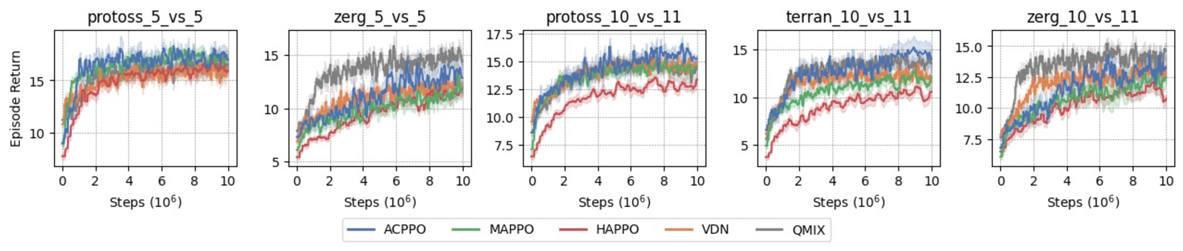
Figure 11: Return for SMACv2 with mean and standard error over 5 seeds..
18 Off-Policy Comparison↩︎

Figure 12: Comparison of Off-Policy Algorithms on MA-MuJoCo (Gymnasium)..
We further evaluate an off-policy variant of ACPO, referred to as ACTD3, following the on-policy experiments. ACTD3 applies the agent-chaining mechanism to TD3 [20]. As off-policy baselines, we compare against MADDPG [11] and HATD3 [15]. As shown in Figure 12, ACTD3 achieves performance comparable to or better than the baseline methods across different tasks. The performance gap is the highest for Ant \(4 \times 2\) which is the most challenging domain.
We note that in HalfCheetah tasks, there is a substantial gap in episode returns between the on-policy and off-policy experiments. Similar discrepancies have been reported in prior works [46], [47] in single-agent experiments on MuJoCo. We attribute this discrepancy to the fundamental differences between on-policy and off-policy learning paradigms. On-policy methods update policies using trajectories generated by the current policy, whereas off-policy methods learn from transitions sampled from a replay buffer containing experiences collected by past policies. The ability to reuse past experiences enables off-policy methods to perform multiple gradient updates per environment interaction, which often results in better sample complexity.
Finally, we note that MA-MuJoCo (Gymnasium) is a more recent benchmark in comparison to MA-MuJoCo (Gym) where the underlying physics engine uses Gymnasium/MuJoCo-v5 and Gym/MuJoCo-v2, respectively. As previous work such as [15] used the older version of MA-MuJoCo (Gym), the results from their paper cannot be directly compared to ours.
19 Wall-Clock Training Time↩︎
19.0.0.1 Runtime Statistics

In Figure 13, we show the wall-clock training time of running MAPPO, HAPPO, HATRPO and ACPO on RWARE for 5M timesteps. With the number of agents increasing from 2 to 12, the runtime of ACPO remains comparable to MAPPO, and is substantially faster than alternating policy optimization methods such as HAPPO and HATRPO, which require alternately updating one agent at a time. Overall, ACPO significantly outperforms baselines in terms of return with only minimal additional computational overhead compared to MAPPO.
20 Hyperparameter Details↩︎
For a fair comparison, we set the network type (MLP or GRU) and hidden layer size to be consistent across all algorithms. The total number of parameters used by ACPPO are set to be similar to that of other algorithms. The design choices follow the experimental setups of [15] and [32]. The discount factor \(\gamma\) is fixed, as it is inherent to the MMDP rather than a tunable hyperparameter. In contrast ACPO employs serialization, where the advantage is computed using \(\gamma' = \gamma^{1/N}\).
\begin{table}[h!]
{| Parameter | RWARE | MA-MuJoCo (on-policy) | MA-MuJoCo (off-policy) | SMACv2 |
|---|---|---|---|---|
| Network | MLP | MLP | MLP | GRU |
| Hidden Sizes (48) | [128, 256] | [256, 256] | [128, 128] | [64] |
| \(\gamma\) | 0.99 | 0.99 | 0.99 | 0.99 |
-0.1in \end{table}
\begin{table}[h!]
{| Parameter | RWARE | MA-MuJoCo (on-policy) | MA-MuJoCo (off-policy) | SMACv2 |
|---|---|---|---|---|
| Network | MLP | MLP | MLP | GRU |
| Hidden Sizes | [128, 128] | [256, 256] | [128, 128] | [48] |
| Hidden Sizes (Action Belief Network) | [64, 64] | \(-\) | \(-\) | [48, 48] |
| \(\gamma\) | 0.99 | 0.99 | 0.99 | 0.99 |
-0.1in \end{table}
For all baselines, we use the reported hyperparameters from [32] for RWARE, [33] for SMACv2 and tune additional hyperparameters for HAPPO and HATRPO for MA-MuJoCo (Gymnasium) on top of the default hyperparameters from [15] for MA-MuJoCo (Gym).
21 Computational Resources↩︎
For RWARE experiments, we utilized a single NVIDIA GeForce RTX 3090 graphics processing unit (GPU). The training times varied across algorithms and the number of agents. For the 2,4,8, and 12-agent environments, ACPO took 14H, 19H, 20H and 23H, respectively. The corresponding times were MAPPO (4H, 6H, 13H, 16H), HAPPO (16H, 32H, 66H, 82H) and HATRPO (18H, 30H, 59H, 90H).
References↩︎
In game theory terminology, the optimal joint policy in cooperative MARL is the social optimum that maximizes welfare.↩︎
This parameterization encompasses both algorithms for learning stochastic policies [10] and deterministic target policies with a stochastic behavior policy [20].↩︎
Knowledge of other agents’ policies is a standard assumption in game theory. In practice, \(\vec{\varphi}^{<i}_t\) can be computed exactly by querying a shared policy with each preceding agent’s index, or by maintaining copies of the preceding agents’ policies. In partially observable settings it must be approximated (Section 4.2).↩︎
We do not compare HATRPO on SMACv2 as it is estimated to take up to 40 days for training, which exceeds our computational budget for this work. Moreover, the results from [15] showed HATRPO is a weaker baseline in SMACv2 in comparison to HAPPO, MAPPO and QMIX. Further details are provided in Appendix 21.↩︎
Note that we also compared with QMIX [17] on RWARE. However, as QMIX failed to learn any meaningful behavior, we do not report their full results. This is consistent with the results reported in [32], and shows the limitations of value decomposition assumptions in complex coordination tasks.↩︎
CTDS is also referred to as Decentralizing Centralizing Solutions [38].↩︎