Optimizing Expert-Designed Crystal Graph Networks for Band-Gap Prediction
with an Autonomous LLM Research Loop
June 29, 2026
Abstract
Predicting a material’s properties from its structure is a central, fast-advancing problem in computational materials science. A decade of work has produced standard public benchmarks and many published machine-learning models for the task [1]. The task’s fixed metric and these baselines make it a natural setting for autonomous agent research [2]. On the MatBench band-gap benchmark (\(>\)100k crystals), a general-purpose coding agent autonomously built the most accurate model trained without external pretraining, ahead of all seventeen expert-designed models reported for the task. A closer analysis shows it reached this by implementing known methods: either already standard in crystal neural-network models, or borrowed from other areas of machine learning. The contributing implementations include element-pair features on each message-passing edge and a crystal space-group embedding. The work not only demonstrates that LLM-agent autonomous research can optimize an expert-designed machine learning model for material property prediction, but also investigates the limitations of such autonomous research.
1 Introduction↩︎
Predicting a crystal’s properties from its atomic structure is a central problem in computational materials science. A decade of work has produced standardized public benchmarks, from single-property suites [1] to stability prediction built on machine-learned interatomic potentials (learned models of a structure’s energy) [3], together with a large body of published models evaluated against them [4], [5]. The most successful of these frameworks are graph neural networks, which represent a crystal as atoms joined by bonds and so build in the local geometry. These networks are expert-designed from physical reasoning, for example: [6] encoded each atom’s local chemical environment in a crystal graph, [7] used continuous-filter convolutions so a predicted energy varies smoothly as the atoms move, and [8] added a line graph to encode the bond angles that many properties depend on.
A fixed metric and a field of expert-designed baselines are the conditions an autonomous research agent is built to exploit. Autonomous, agent-driven research has advanced quickly, with recent systems running full machine-learning research pipelines end to end [9], [10]. That progress, however, has stayed mostly within machine learning and computer science. Whether an LLM-driven coding agent can do the same on a materials-science question has not been established. Success there needs two things: writing correct code, which these agents handle increasingly well [11]–[13], and the scientific judgment to turn each result into the next modeling decision.
We therefore use the MatBench benchmark [1] as a test field for this question, focusing on its band-gap task: more than 100,000 crystals and more than twenty published models with reported scores. We minimize the agent’s workflow: each experiment edits a training script, costs real compute, and returns only a single held-out number, with no human in the loop [2]. The result is surprising: with no materials-specific design, the agent built the most accurate model trained without external pretraining, ahead of all seventeen such from-scratch models reported for the task (Figure 1). Analyzing the final model shows that this improvement came from recombining existing methods rather than inventing new ones. The methods it recombined are of two kinds, those already existing in standard crystal neural networks and those borrowed from other areas of machine learning, and the result follows from combining them rather than from any single one (Figure 2, Table 1).
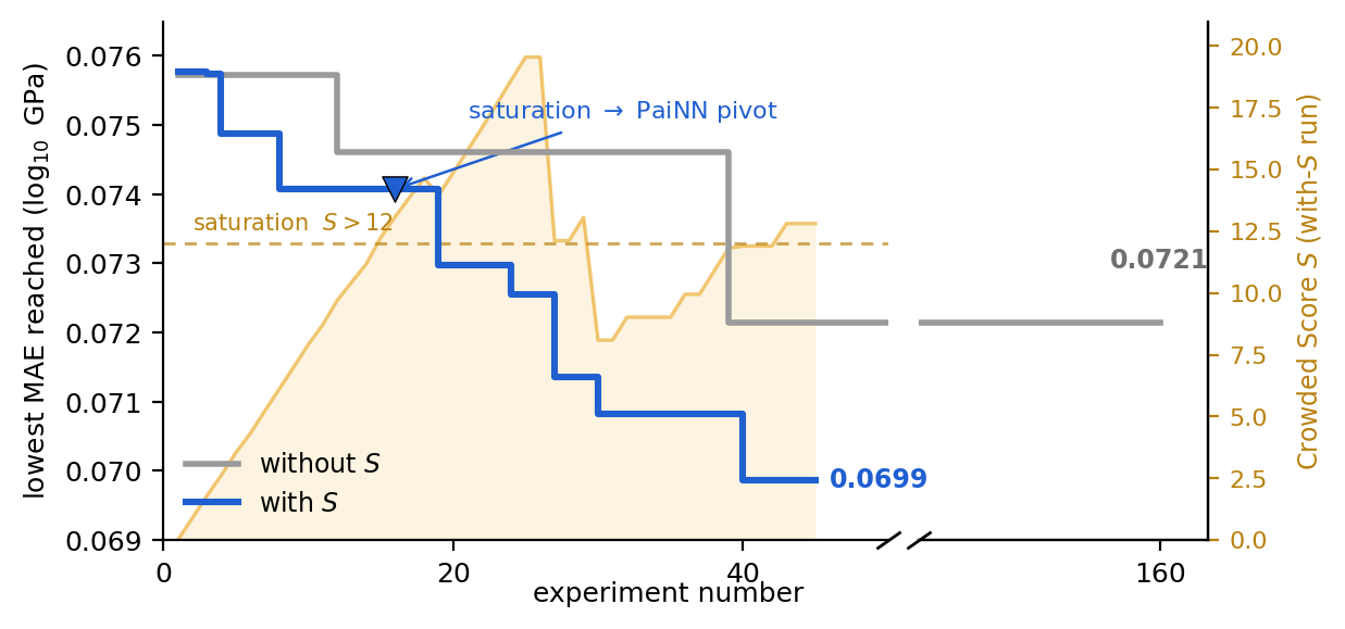
We also find a limitation of these loops: the agent keeps making small changes to one model and stops improving, instead of exploring a different approach. Other autonomous research agents address the same problem with different strategies: for example, an evolutionary population of programs in AlphaEvolve [14], and Monte Carlo tree search over candidate solutions in AB-MCTS [15] and the AI Scientist [10]. Here we use a simpler method: a crowding score that measures how much the best model so far makes the same mistakes as other equally accurate models, and asks the agent to try a different approach when that score is high. With the crowding score, on a second task (shear-modulus prediction), the loop reaches a mean absolute error of \(0.0699\) in \(\log_{10}\) GPa by experiment \(40\), while the same loop without it never gets below \(0.0721\) across all \(160\) experiments (Section 5).
![Figure 1: Mean absolute error (eV, log scale, lower is better) on the mp_gap task for the agent’s best model (gold star), compared against published methods at their reported scores from the public MatBench leaderboard or source paper [1]. Blue circles mark from-scratch single-task crystal graph neural networks: coGN and coNGN [5], CrysToGraph [16], DenseGNN [17], DeeperGATGNN [18], ALIGNN [8], MEGNet [4], DimeNet++ [19], SchNet [7], MatInFormer [20], CGCNN [6], and Matini-Net [21]. Orange triangles mark foundation-model methods that import external large-scale pretraining: JMP [22], TriForces [23], MatterVial [24], and CLOUD [25]. Grey squares mark composition or other baseline models: Finder [26], MODNet [27], CrabNet [28], AMMExpress v2020 [1], and RF-SCM/Magpie [29].](/article/2606.29717/figures/f1_comparison.png "fig:")
2 Experimental Setup↩︎
The main task we used is mp_gap [1]: predict the electronic band gap in eV from a crystal structure, scored as the mean
absolute error over a fixed five-fold partition of more than \(100{,}000\) crystals. The standard reference on this task is coGN [5], a crystal graph network built on an optimized way of connecting the atoms into a graph, at \(0.1559\) eV. Two newer crystal graph networks report lower error: CrysToGraph at \(0.1522\) eV [16], and DenseGNN, which adds dense connections between layers, at \(0.1548\) eV [17]. These are among the published models we compare against (Figure 1).
Our loop follows the autonomous-research setup of [2]: the agent edits the training code, the edited model is trained
under a fixed budget, the change is kept or dropped by its measured accuracy, and the loop repeats. In addition to this conventional procedure, we require a change to lower the held-out mean absolute error by more than \(\tau =
0.002\) eV to count as a real improvement, not run-to-run noise. Each training run is capped at \(1{,}500\) seconds (25 minutes) on a single RTX 2070 SUPER GPU, and each candidate model is limited to about five
million parameters, so every experiment finishes quickly and the loop can run hundreds of them. We use Claude Code as the agent, running Claude Opus 4.8 at its highest thinking-effort setting (max). During the search, each candidate is ranked
on a single held-out fold (fold 0). After the loop ends, we take the lowest-error model as the final model and train it on the official five-fold split, \(9{,}000\) seconds per fold, to report its accuracy fully trained
rather than under the search budget. Throughout the loop, the agent edits only the model code, while data loading, the held-out fold, and the error computation are run by fixed scripts the agent cannot change, so every candidate is judged the same way.
In Section 5 we use a second task, log_gvrh, which predicts the base-ten logarithm of the shear modulus in GPa. This task has far fewer crystals (\(\sim\)11,000), so each
model trains quickly and we cut the per-run budget to \(180\) seconds. The smaller budget lets us run many experiments cheaply and focus on developing the agent’s workflow. Apart from the task, its data, and this budget,
the loop and the fixed scripts are the same as for the band-gap task.
3 A competitive model assembled from known methods↩︎
Figure 1 compares the loop’s final model with the published models for the task, each shown at its reported mean absolute error on the official benchmark. The model reaches a mean absolute error of \(0.1480 \pm 0.003\) eV, ranking 6th in the figure. The five models ahead of it (orange triangles) all rely on external pretraining. Four are foundation models pretrained on additional data, JMP-L and JMP-S [22] and TriForces-Orb and TriForces-eSEN [23]. The fifth, MatterVial [24], imports features from other pretrained models. Among the models trained from scratch on this task alone, the loop’s model (marked as the gold star) is more accurate than every expert-designed one.
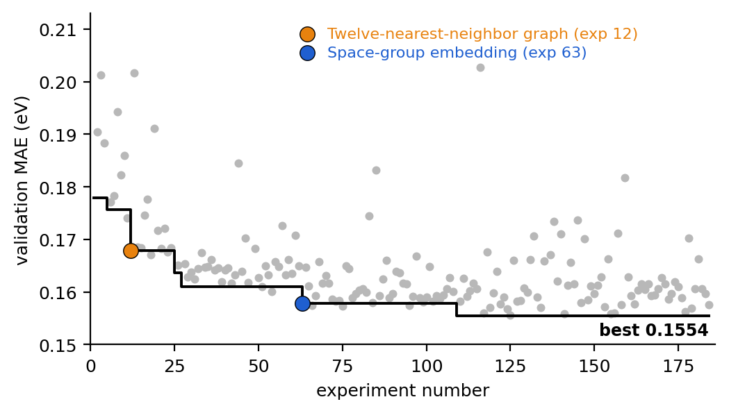
Figure 2 shows the agent’s exploration over 184 experiments. The solid line shows the best held-out MAE kept so far. The line decreases when an experiment’s MAE is at least \(0.002\) eV below the current best, for example the bond-angle and connectivity change at experiment 12 (to \(0.1679\) eV) and the space-group symmetry change at experiment 63 (to \(0.1578\) eV). The grey dots are the attempts that did not improve on the best and were discarded. Seven kept changes in all bring the model from its untuned baseline near \(0.18\) eV to its best model at \(0.1554\) eV, listed in order in Table 2. Two are increases in the model width with no associated method. The rest are representational changes, each matching a method already in the crystal-network literature. The largest single gain adds bond-angle messages through a line graph (a graph whose nodes are the edges of the crystal graph, so the model can use the angles between bonds), the construction used by ALIGNN and DimeNet++ [8], [19], together with a learned nearest-neighbour connectivity in the style of coGN [5]. The later changes add element-pair features on each edge, a space-group embedding for crystal symmetry in the manner of MEGNet’s global features [4], and a wider Gaussian basis for the interatomic distances. Together, these changes make a single crystal graph network that recombines methods from several published models, with its full architecture in Appendix 8.
| Methods proposed | Rediscovery | Cross-domain | Novel | Total |
|---|---|---|---|---|
| Accepted | 5 | 0 | 0 | 5 |
| Discarded | 20 | 5 | 0 | 25 |
| Total | 25 | 5 | 0 | 30 |
To track where the agent’s ideas came from, we analyzed every attempt it made, including the discarded ones, and classified them into three classes by the novelty of each idea. First we identified the real algorithm changes, setting aside pure hyperparameter sweeps such as width or learning-rate changes. This left 30 distinct methods. We then compared each against a reference set of 21 papers from this field, the published models of Figure 1 among them (Table 1, with per-change sources in Appendix 9). A method is a rediscovery if it already appears in one of the crystal graph networks, a cross-domain import if it is absent from them but taken from feature-based materials machine learning or general deep learning, and novel if it appears in neither. All 5 accepted changes are rediscoveries, and 20 of the 25 the loop tried and reverted are also rediscoveries. The remaining 5 are cross-domain imports. They add an inverse-distance Coulomb edge, an element-product edge, and a per-atom neighbor-composition descriptor, train with a robust regression loss, and apply stochastic depth. None of the 30 is novel. The competitive model of Figure 1 is therefore built by recombining known methods alone.
4 The model does not transfer to other tasks↩︎
The band gap is only one of many properties that can be predicted from a crystal’s structure. One may therefore ask whether our model, optimized for band-gap prediction, also predicts other properties well. To answer this, we keep the final model’s
architecture and hyperparameters fixed and retrain it on four other MatBench tasks: elastic-modulus prediction (log_gvrh and log_kvrh) and formation-energy prediction (mp_e_form and perovskites). We chose
these four because each predicts a property from a crystal’s structure, the same kind of task as the band gap.
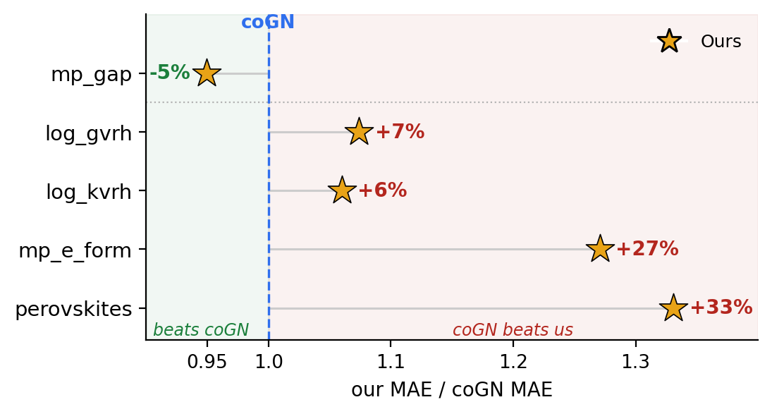
Figure 3 compares our model’s mean absolute error with that of coGN, an expert-designed crystal graph network, on the band gap and the four other tasks. We compare against coGN because it is one of the strongest models
across these tasks and is a single general design: its authors found one architecture and one set of hyperparameters by optimizing on a single task, log_gvrh, then applied them unchanged to every other task with no per-task tuning [5]. They report that this one configuration carries over to the other MatBench datasets and tasks, and attribute its accuracy to an optimized choice of
which atoms are joined in the graph and to deeper message-passing layers. As shown in Figure 3, our model beats coGN on the band gap but loses to it on all four other tasks, by six to thirty-three percent. On those four
tasks the retrained model places 5th, 4th, 4th, and 8th respectively among the established MatBench submissions, an ordinary mid-leaderboard standing rather than a leading one like coGN. These results indicate that the loop produced a model tuned to the
band gap: its standing comes from automated search and tuning on a single task, not from a design that holds across tasks. An expert-designed model like coGN instead rests on a general design choice grounded in crystal structure, how atoms are connected in
the graph, which is why its single configuration transfers where our search-tuned model does not.
5 Getting the agent to try new models↩︎
In the mp_gap task, the AI agent lowered its error quickly at first and then stopped: its best model reached its lowest error after about one hundred experiments and did not improve over the rest of the run. The agent kept refining one
model it had already tuned well, rather than trying a different kind of model. This pattern is clearer on a second task, log_gvrh, which predicts the base-ten logarithm of the shear modulus in GPa. Seeded with the best mp_gap
model retrained on this task at about \(0.076\), the agent lowered the error to \(0.0721\) by about experiment \(40\), then ran more than one hundred further
experiments without lowering it again (Figure 4, grey). It stayed there because the agent kept making small changes to the same model, adjusting its learning rate, width, depth, or optimizer, and never tried a different one,
such as a different graph structure or feature embedding. How to explore the space of possible solutions efficiently is a central question for automated research agents, and different systems answer it differently. AlphaEvolve [14] uses an evolutionary database based on MAP-Elites and island models, and AB-MCTS [15] uses Thompson sampling to choose between a new candidate and a refinement.
Rather than rebuild the search like those systems, here we apply a simpler approach. We compute a single quantity, the crowding score \(S(e)\) for each committed model \(e\), to measure how much model \(e\) repeats the models already tried and to prompt the agent to propose a new idea when \(S\) is high. The score is defined as \[S(e) \;=\; \sum_{\substack{f \neq e \\ |\mathrm{MAE}_e - \mathrm{MAE}_f| \,<\, \tau}} \max\!\bigl(0,\; \rho(\mathbf{r}_e, \mathbf{r}_f)\bigr), \qquad \tau = 0.004, \label{eq:crowded}\tag{1}\] where \(\mathbf{r}_e = \hat{\mathbf{y}}_e - \mathbf{y}\) is model \(e\)’s vector of per-crystal errors on a fixed held-out set, \(\mathrm{MAE}_e = \mathrm{mean}(|\mathbf{r}_e|)\) is its mean absolute error, \(\rho\) is the Pearson correlation between two such vectors, and the sum runs over every other committed model whose error is within \(\tau\) of \(e\)’s. A model’s residual vector is its fingerprint, so two highly similar models produce residual vectors that are highly correlated, giving a high \(\rho\). When the loop only makes small changes to the best model, it produces many new models that are highly similar to it. Each of these has a high \(\rho\) with the best model, so the best model’s score \(S\) rises quickly. Once the best model has \(S > 12\), we tell the agent to stop refining it and build a different kind of model. The score is computed by the harness from residuals the agent never sees, and it is the only thing added to the loop. With the score fed back, the loop’s convolution models grew crowded enough to pass the threshold at experiment \(15\), and the agent switched to a PaiNN-style equivariant network, one that carries directional vector features alongside the usual scalar ones [30], at experiment \(16\). That first version scored worse than the convolution models, but after a few refinements it passed their best at experiment \(19\) and reached \(0.0699\) by experiment \(40\), below the \(0.0721\) the run without the score never passed despite running more than three times as many experiments (Figure 4).
6 Related work↩︎
Band-gap models for this task. Predicting the band gap from crystal structure is an established machine-learning task with many published models (Figure 1), ranging from message-passing crystal graph networks to foundation models pretrained on additional data. Among the models trained without external pretraining, the loop’s model reaches the lowest reported error. References for the compared models are listed in that figure’s caption.
Autonomous research loops. LLM agents that propose, run, and keep code changes against a held-out metric have been built for machine-learning engineering: [31] frame the work as a tree search over training code, and [32] study the search policy and operator set that such loops use. Related systems automate a wider research cycle [9] or evolve programs that improve on the best known algorithm [14], [33]. These systems were demonstrated on machine-learning, coding, and mathematics benchmarks, where a helpful change is a general code or training adjustment. We instead apply such a loop to a materials-property benchmark, which calls for domain knowledge of crystal structure, chemical bonding, and space-group symmetry rather than a general code change. LLM agents in materials science have largely proposed new compounds and synthesis routes [34], [35] rather than optimizing a property-prediction model, so what such a loop converges on for this task has not, to our knowledge, been characterized.
7 Conclusion↩︎
In this work, we investigate whether a general-purpose coding agent, run as an autonomous loop on a mature materials benchmark, can produce a model competitive with expert-designed ones. On the band-gap task, the loop built the most accurate model trained from scratch, ahead of every expert-designed one, by assembling existing methods rather than inventing a new one. This result indicates that a simple autonomous LLM research loop can optimize an expert-designed model and improve its accuracy. Two limitations remain: (a) the model the agent optimized does not transfer to other tasks, unlike an expert-designed model built from physical reasoning such as coGN, and (b) the agent tends to stop improving, making small adjustments rather than exploring a different approach. For the second limitation, we propose the crowding score, a scalar that measures the extent to which the current best model repeats the errors of other equally accurate models. When this score is high, we prompt the agent to develop a different class of model. With the crowding score, the loop reached a lower error than the same loop run without it. Applying the same loop beyond band-gap prediction, to other graph-network model families such as machine-learning interatomic potentials and foundation models for materials, is a direction for future work.
8 Final model architecture↩︎
The final model (about \(503{,}617\) parameters) is a crystal graph network with width \(120\) and four message-passing layers. A crystal is converted to a graph with a \(5.0\) Å cutoff and a \(k\)-nearest-neighbour cap of \(12\) (the connectivity primitive). Each edge carries a \(32\)-component Gaussian radial basis of the interatomic distance together with the element pair of its endpoints (the distance and composition primitives). One ALIGNN-lite update passes angle-aware messages between bonds that share an atom, using a line graph and an \(8\)-component basis of the bond-angle cosine (the angle primitive). Four CGCNN-style gated convolutions [6] update the atom states. A global term concatenates six lattice and density statistics with a \(16\)-dimensional embedding of the space group, one of \(231\) (the symmetry primitive). Readout pools the atom states by mean and max, appends the global term, and regresses the band gap. Weights are trained with Adam under a cosine schedule, and predictions use an exponential moving average of the weights.
9 Kept changes and their provenance↩︎
Table 2 lists the kept changes of the reported search, in order. Table 3 lists the cross-domain methods the agent tried and reverted.
| Exp. | MAE (eV) | Change | Primitive | Prior source (rediscovery) |
|---|---|---|---|---|
| 1 | 0.1780 | seed baseline | distances | – |
| 5 | 0.1757 | width \(64 \to 96\) | capacity | – |
| 12 | 0.1679 | \(k\)-NN cap \(K{=}12\) and ALIGNN-style angle update | connectivity, angles | CGCNN [6]; ALIGNN [8], DimeNet++ [19] |
| 25 | 0.1636 | element-pair features in the edge MLP | composition | MEGNet [4] |
| 27 | 0.1610 | width \(96 \to 112\) | capacity | – |
| 63 | 0.1578 | space-group embedding and width \(120\) | symmetry | CLOUD [25], Automatminer [1] |
| 109 | 0.1554 | wider Gaussian radial basis (final model) | distances | SchNet [7] |
| Exp. | Cross-domain import (tried, reverted) | Prior source |
|---|---|---|
| 42 | Per-atom neighbor-composition descriptor | MatterVial [24] |
| 92 | Element-product edge | MatterVial [24], CrabNet [28] |
| 126 | Robust regression loss | CrabNet [28], FINDER [26] |
| 151 | Inverse-distance Coulomb edge | MatterVial [24] |
| 169 | Stochastic depth | general deep learning [36] |
10 Prompts with crowding score↩︎
Below is program.md, the full prompt that defines the agent’s loop in the crowding-score run of Section 5.
autoresearch – log_gvrh (novelty-driven, representation-first)
You are a creative materials-science ML researcher. Goal: the LOWEST mae: (log10 GPa) on matbench_log_gvrh, the official held-out fold, under a fixed compute budget. You edit ONE file (train.py), run it, and commit it. There is
NO reset – every model is committed and KEPT IN HISTORY so novelty.py can fingerprint it. But you always REFINE FROM THE BEST model so far (lowest mae), never from whatever was committed last (see "Each round"). The best model is recovered at the end. Loop
until interrupted.
Setup (once)
Read
prepare.py(READ-ONLY: data, official fold, private TEST labels, the MAE metric – never edit it, never readdata/*directly) andtrain.py(the ONLY file you edit).ref/has real installed reference code if you want it (matgl line-graph / three-body utils, coGN / coNGN / ALIGNN) – take ideas, do not copy; you are not limited to known approaches.Create
results.tsvwith the header if missing (see Logging).
You are a scientist, not a tuner
Your job is to understand why the current model fails and to invent a better one – any representation, architecture, or inductive bias you think could work. Do not limit yourself to known or conventional approaches; pursue whatever ideas you find genuinely promising, including ambitious or unconventional ones. Depth of understanding over number of edits; aim for novelty.
Each round
STUDY: read
novelty_report.md–S(a)(how behaviorally crowded the model you develop from – the best method so far – is: how many same-scoring models already make the same predictions as it) and whether it is SATURATED (S(a) > 12). The "most crowded models" list shows redundancy across the whole family. When you need to diverge, read theresults.tsvdescriptions to see which mechanisms already exist.INTERPRET: think through what the best model is failing to capture, and why. Reason from the physics of elasticity and bonding where it helps. Understanding first; edits second.
DECIDE:
NOT saturated and you have a concrete improvement \(\rightarrow\) refine the best model.
SATURATED (
S(a) > 12– the family keeps building near-duplicates that score the same and make the same mistakes) \(\rightarrow\) STOP refining; this mechanism is exhausted. Invent a fundamentally different model, one NOT in the crowded clustersnovelty_report.mdnames. A coupled change touching several parts oftrain.pyat once is expected.
IMPLEMENT: FIRST run
bash checkout_best.sh– it restorestrain.pyto the best (lowest-mae) model so far, so you build on the STRONGEST model, not whatever was committed last. It changes only the working file; every commit stays in history. Run it BEFORE editing – running it after would discard your edit. THEN edit ONLYtrain.pyon top of the restored best.RUN, then COMMIT, then LOG – the order matters (see below).
Run / commit / log (order matters)
bash checkout_best.sh                                  # FIRST: restore train.py to the best model
# ... now edit train.py ...
source .venv/bin/activate
python train.py > run.log 2>&1
grep "^mae:\|^num_params:\|^peak_vram_mb:" run.log     # empty mae => crash (tail run.log)
git add -A && git commit -m "<one-line reasoning: mechanism + hypothesis>"
RUN, then COMMIT: the run stages this model’s fingerprint. THEN commit – the post-commit hook keys the fingerprint by the new commit and rewrites
novelty_report.md. Never skip the commit.After committing, append a
results.tsvrow:git rev-parse --short HEAD, the mae, peak_vram, a one-line mechanism + hypothesis description. That description is your durable memory – make it specific (your fuller reasoning goes in the commit message).
CAN / CANNOT
CAN (all in train.py): featurization (cutoff, connectivity, line graphs / bond angles, node / edge / global features, multiple graphs per crystal), model, optimizer, schedule, training loop, batch size, readout. CANNOT: edit
prepare.py; change the data / fold split / TEST labels / prepare.evaluate_mae metric; read data/* or fingerprints/* directly; install packages (import what is already installed); exceed 5,000,000 params
(print num_params); touch run.sh, the git hooks, novelty.py, checkout_best.sh, tmux, or any process but python train.py; end this session.
Hard constraints
ENVELOPE – matched, not scaled: \(\leq\) 5M params, single GPU, FP16 ok. A win must be algorithmic / representational. Heavier graphs (line / three-body) train fewer steps in the fixed budget – that is the rule; if a richer model is close but under-trained, shrink it rather than drop the idea.
FIXED BUDGET – each run trains
prepare.TIME_BUDGETs (180), then evaluates.FIXED SEED –
train.pyseeds RNG at the top so one run is a fair comparison. Keep it.FEAT CACHE –
featurize()caches perFEAT_KEYunderprepare.cache_dir(FEAT_KEY). CHANGEFEAT_KEYwhenever featurize() output changes, or you read a stale cache.feat_secondsis printed and does NOT count against the budget.
Logging (results.tsv, TAB-separated)
commit mae memory_gb status descriptionshort-hash mae (0.000000 if crash) peak_vram_mb/1024 keep (always – no reset) or crash one-line mechanism + hypothesis.
Baseline
Iteration 1 = the seed train.py AS IS: run once, commit, log (status keep). Change nothing before it is recorded. If results.tsv already lists kept models, the baseline is done – do NOT repeat it; continue the loop.
novelty_report.md is empty until after the first commit – that is expected.
Crashes
Trivial (typo / import) \(\rightarrow\) fix and re-run. Fundamentally broken \(\rightarrow\) log mae 0.000000, commit anyway so history stays complete, move on. NaN pooled
stats are common – clamp variances, avoid dividing by zero atom counts. Line-graph / three-body code is crash-prone; build incrementally, keep FEAT_KEY in sync.