Fourier–Hankel Moment Methods for Topological Counting and Phase-Center Recovery in Acoustic Inverse Scattering
June 29, 2026
Abstract
We develop a Fourier–Hankel moment framework for extracting topological counting information from full-aperture acoustic far-field data. The method is based on the observation that separated localized components generate distinct phase centers in angular Fourier data. Under the Born approximation, a Bessel–Fourier moment identity shows that suitably scaled row Fourier coefficients form, to leading order, a finite exponential moment sequence. The associated Hankel matrix has rank equal to the number of separated connected components, and the corresponding Hankel pencil recovers their phase-center locations. We prove the exact Hankel rank formula in the phase-center model and establish a perturbation theorem showing stable component counting under a singular-gap condition. We further extend the framework to detectable cavities by introducing a signed phase-center model. In this model, material components and cavities contribute with opposite signs to the moment sequence. The signed Hankel rank counts distinct signed phase centers, and the detectable cavity count is obtained from the excess rank beyond the positive component count. This formulation also identifies an intrinsic degeneracy: cavities whose phase centers coincide with material phase centers, such as perfectly concentric annuli, do not increase the leading signed rank and therefore cannot be detected by the leading phase-center mechanism alone. Numerical experiments validate the proposed theory at several levels: ideal moment sequences, Born far-field data with finite-size components, phase-center location recovery, signed cavity counting, and exact Helmholtz far-field data. The results show that the Fourier–Hankel rank mechanism provides a data-level algebraic approach to component counting and detectable cavity counting, while also making explicit its stability conditions and failure modes.
Keywords: acoustic inverse scattering; Fourier–Hankel moments; Hankel matrices; Betti number; Prony method
1 Introduction↩︎
The inverse acoustic scattering problem seeks to determine information about an unknown obstacle or inhomogeneity from the waves it scatters. In the full-aperture multistatic setting, the data are far-field patterns measured for pairs of incident and observation directions at one or several frequencies. This problem is a classical topic in inverse scattering theory and has been studied extensively because of its relevance to nondestructive testing, sonar imaging, medical diagnostics, and other wave-based imaging applications; see, for instance, the monographs of Colton and Kress [1] and Kirsch [2].
Mathematically, acoustic inverse scattering is nonlinear and severely ill-posed: small perturbations of the measured wave field may lead to significant uncertainty in the recovered geometry or material contrast. This has led to a broad range of reconstruction methodologies developed to tackle the inherent nonlinearity and ill-posedness of this inverse problem. These approaches span a rich spectrum, ranging from computationally efficient qualitative techniques to high-fidelity iterative optimization schemes. Among them, sampling-type and qualitative methods—such as the linear sampling, factorization, and probe methods—have gained prominent traction for their ability to fast-localize scatterers or map their geometries without undergoing expensive nonlinear optimization [3]–[8]. This paradigm has been further expanded by direct and extended sampling methods, which offer robust, non-iterative imaging capabilities even under constrained configurations like limited apertures or single-incident waves [9]–[12]. Conversely, when precise boundary profiles or contrast distributions are required, optimization-based framework and Newton-type iterative solvers are typically deployed to minimize data-misfit functionals, leveraging tailored regularization techniques and shape derivatives to stabilize the inversion [13]–[16]. Statistical and Bayesian approaches provide another important framework, in which uncertainty in the unknown scatterer and in the measured data is incorporated into the inverse problem through prior distributions, posterior inference, and uncertainty quantification [17]–[19]. To bridge the gap between theoretical frameworks and practical engineering, sustained research efforts have long focused on multi-frequency data fusion, limited-aperture constraints, and resolution enhancements [12], [20], [21], substantially elevating the robustness of acoustic scattering measurements in complex environments.
The present paper addresses a different but related imaging question. Instead of attempting to reconstruct the full boundary or contrast, we ask whether certain low-dimensional geometric and topological features can be extracted directly from the far-field data. In particular, we focus on the number of separated connected components, the recovery of their dominant phase-center locations, and the counting of detectable cavity phase centers. Such information is discrete or skeleton-like in nature. It may be difficult to infer robustly from a thresholded reconstructed image or from a qualitative indicator alone, especially when components are close, cavities are small, or the data are noisy. This motivates a data-level spectral approach, in which the angular structure of the far-field pattern is transformed into moment sequences whose Hankel ranks and matrix pencils encode the desired counting and localization information.
Our approach is closely related to the literature on small scatterers, point-like targets, and subspace imaging. Small-volume asymptotic theory and polarization tensor methods show that localized inhomogeneities leave finite-dimensional signatures in boundary or far-field measurements [22], [23]. MUSIC and related subspace methods exploit the finite-dimensional structure of multistatic response data to locate small or point-like scatterers [24], [25]. These works indicate that, in suitable regimes, scattering data may contain algebraic structures associated with localized objects.
A second related line of work is moment, Prony, and Hankel-type reconstruction. Classical Prony and matrix pencil methods recover finite exponential sums from sampled moments by exploiting annihilating polynomials, Vandermonde factorizations, or Hankel rank conditions [26]–[30]. Similar algebraic structures also arise in inverse source problems, where point sources or multipoles generate finite-dimensional moment systems [31], [32]. More recently, Hankel determinant and contour-counting principles have been used to identify the number of stationary point sources in inverse heat source problems [33], [34]. Although these problems differ from inverse acoustic scattering, they suggest a useful principle: if measured data can be transformed into a finite exponential-moment representation, then counting and localization of hidden objects may be possible at the data level.
For acoustic inverse scattering, the relevant phase information is contained in the angular dependence of the far-field pattern. Under the Born approximation, the far-field pattern is related to the Fourier transform of the scattering contrast. By expanding the multistatic far-field matrix with respect to the observation and incident angles, one obtains Bessel–Fourier moments of the weighted contrast. We show that a suitable low-order row channel of these coefficients, after a Bessel leading-order scaling, has the form of a finite exponential moment sequence in the localized phase-center regime. The associated Hankel matrix then admits a Vandermonde factorization. Consequently, its rank equals the number of separated phase centers, and hence the number of connected components under the separated localized component model.
The same moment structure also yields a Hankel-pencil procedure for recovering the component phase-center locations. This should be understood as a skeleton-type recovery of dominant scattering centers, rather than a full boundary reconstruction. We further extend the framework to cavities by introducing a signed phase-center model. In this model, material regions and cavities contribute with opposite signs to the leading moment sequence. The signed Hankel rank counts the number of distinct signed phase centers, while the excess over the positive component count gives the number of detectable cavity phase centers. This distinction is essential: a physical cavity is not always detectable by the leading signed-rank mechanism. For example, in a perfectly concentric annulus, the positive material phase center and the negative cavity phase center coincide, so their leading contributions collapse into a single phase node. Such degenerate cavities require higher-order radial information, additional Fourier–Bessel channels, or multiple-frequency information beyond the leading phase-center model.
The contribution of this paper is to develop a Fourier–Hankel moment framework for component counting, phase-center localization, and detectable cavity counting from acoustic far-field data. We first derive a Bessel–Fourier moment identity for the angular Fourier coefficients of the far-field pattern. We then prove an exact Hankel-rank formula for component counting in the localized phase-center model and establish a perturbation theorem showing that the count is stable under a singular-gap condition. We also derive a Hankel-pencil recovery formula for phase-center locations. Finally, we introduce a signed phase-center extension for cavity counting and clarify its detectability condition and degeneracy mechanism.
Numerical experiments are designed to match these theoretical claims. We test the algebraic Hankel-rank mechanism on ideal moment sequences, component counting from Born far-field data with finite-size components and noise, phase-center location recovery through the Hankel pencil, signed phase-center cavity counting, and component counting from exact Helmholtz far-field data. The experiments show that the proposed Fourier–Hankel construction captures the theoretical rank mechanism and remains effective beyond the idealized moment model in a range of controlled scattering configurations.
The rest of the paper is organized as follows. Section 2 introduces the scattering model, angular Fourier coefficients, and the Fourier–Hankel moment formulation. Section 3 proves the Hankel-rank formula for component counting and the associated stability result. Section 4 develops the signed phase-center extension for detectable cavity counting. Section 5 presents the numerical experiments. Section 6 concludes the paper.
2 Fourier–Hankel moment formulation↩︎
This section introduces the acoustic scattering model and the angular Fourier coefficients used throughout the paper. Our aim here is not to solve the full nonlinear inverse scattering problem, but to identify a moment structure in the far-field data that can be used for component counting. The theoretical derivation is carried out for a penetrable acoustic inhomogeneity under the Born approximation, where the far-field pattern admits a Fourier-transform representation of the contrast. For impenetrable obstacles or fully nonlinear scattering models, the same Fourier–Hankel construction may still serve as a data-level spectral descriptor. However, the exact Hankel-rank formula proved below should be understood as a result for the Born-type phase-center model.
2.1 Scattering model and angular Fourier coefficients↩︎
Let \(D\subset\mathbb{R}^2\) be a bounded inhomogeneity, and let \(q\) be a compactly supported contrast with \(\operatorname{supp}q\subset D\). In what follows, the connected components to be counted are the separated components of the effective contrast support. For an incident plane wave \[\begin{align} u^i(x, d; k)=e^{\mathrm{i}k d\cdot x}, \qquad d\in\mathbb{S}^{1}, \end{align}\] the total field is \[\begin{align} u(x, d; k)=u^i(x, d; k)+u^s(x, d; k), \end{align}\] where \(u^s\) denotes the scattered field and satisfies the Sommerfeld radiation condition. In two dimensions, the scattered field has the far-field asymptotic form \[\begin{align} u^s(x,d;k)=\frac{e^{\mathrm{i}k|x|}}{|x|^{1/2}} \left\{u^\infty(\hat{x},d;k)+O(|x|^{-1})\right\}, \qquad \hat{x}=\frac{x}{|x|}, \qquad |x|\to\infty . \end{align}\] The coefficient \(u^\infty(\hat{x},d;k)\) is the far-field pattern.
For a compactly supported contrast, the far-field pattern admits the representation \[\begin{align} u^\infty(\hat{x}, d; k)=C_k \int_D e^{-\mathrm{i}k\hat{x}\cdot y}q(y)u(y,d;k)\,\mathrm{d}y, \label{eq:farfield95full} \end{align}\tag{1}\] where \(C_k\ne0\) is a known dimensional constant determined by the normalization of the two-dimensional Green function. The precise value of \(C_k\) is immaterial for the rank analysis, since it only rescales the moment sequence.
According to the Born approximation, the total field \(u(y,d;k)\) in 1 is replaced by the incident field \(e^{\mathrm{i}k d\cdot y}\). We then obtain \[\begin{align} u^\infty(\hat{x},d;k) \approx C_k\int_D q(y)e^{-\mathrm{i}k(\hat{x}-d)\cdot y}\,\mathrm{d}y . \label{eq:born95farfield} \end{align}\tag{2}\] Equation 2 shows that, in the Born regime, the far-field pattern contains Fourier information of the weighted support \(q\chi_D\) through the scattering vectors \(k(\hat{x}-d)\). This motivates a direct spectral analysis of the far-field data themselves. In particular, we ask whether geometric and topological information of the scatterer, such as component and cavity information, can be inferred from the angular structure of these data.
For this purpose, we write the far-field pattern in angular variables. Let \(\theta\) and \(\varphi\) denote the observation and incident angles, respectively, and set \[\begin{align} \hat{x}(\theta)=(\cos\theta,\sin\theta), \qquad d(\varphi)=(\cos\varphi,\sin\varphi), \qquad 0\le \theta,\varphi<2\pi . \end{align}\] We write \[\begin{align} u^\infty(\theta,\varphi;k) := u^\infty(\hat{x}(\theta),d(\varphi);k). \end{align}\] The continuous angular Fourier coefficients of the full-aperture far-field matrix are then defined by \[\begin{align} a_{mn}(k)=\frac{1}{(2\pi)^2} \int_0^{2\pi}\int_0^{2\pi} u^\infty(\theta,\varphi;k) e^{-\mathrm{i}m\theta}e^{-\mathrm{i}n\varphi} \,\mathrm{d}\theta\,\mathrm{d}\varphi, \qquad m,n\in\mathbb{Z}. \label{eq:angular95fourier95coeff} \end{align}\tag{3}\]
In computations, the far-field pattern is available only at finitely many angular directions. For uniform samples, let \[\begin{align} \theta_i=\frac{2\pi i}{N_{\rm ang}},\qquad \varphi_j=\frac{2\pi j}{N_{\rm ang}}, \qquad i, j=0,\ldots,N_{\rm ang}-1 . \end{align}\] The empirical angular Fourier coefficients are then \[\begin{align} a_{mn}^{(N_{\rm ang})}(k) = \frac{1}{N_{\rm ang}^2} \sum_{i,j=0}^{N_{\rm ang}-1} u^\infty(\theta_i,\varphi_j;k) e^{-\mathrm{i}m\theta_i}e^{-\mathrm{i}n\varphi_j}. \label{eq:discrete95fourier95coeff} \end{align}\tag{4}\] For simplicity, the same number \(N_{\rm ang}\) of observation and incident directions is used. The extension to unequal numbers of observation and incident directions is straightforward. In the subsequent Hankel construction, only finitely many low-order coefficients are retained.
We now derive the angular moment identity used in the sequel. In polar coordinates \(y=(r\cos\psi,r\sin\psi)\), and using the same symbol \(D\) for the corresponding polar domain, the Born far-field representation 2 becomes \[\begin{align} u^\infty(\theta,\varphi;k) \approx C_k \int_D q(r,\psi) e^{-\mathrm{i}kr\cos(\theta-\psi)} e^{\mathrm{i}kr\cos(\varphi-\psi)} r\,\mathrm{d}r\,\mathrm{d}\psi . \label{eq:born95polar} \end{align}\tag{5}\] Using the Jacobi–Anger expansion \[\begin{align} e^{\mathrm{i}t\cos\omega}=\sum_{\ell\in\mathbb{Z}}\mathrm{i}^\ell J_\ell(t)e^{\mathrm{i}\ell\omega} \label{eq:jacobi95anger} \end{align}\tag{6}\] and the orthogonality of the Fourier basis on the unit circle, taking the \((m, n)\) angular Fourier coefficient of 5 gives the Bessel–Fourier moment identity \[\begin{align} a_{mn}(k)=C_k(-\mathrm{i})^m\mathrm{i}^n \int_D q(r,\;psi)J_m(kr)J_n(kr)e^{-\mathrm{i}(m+n)\psi} r\,\mathrm{d}r\,\mathrm{d}\psi, \qquad m,n\in\mathbb{Z}. \label{eq:bessel95fourier95moment} \end{align}\tag{7}\] The identity 7 shows that \(a_{mn}(k)\) is a Bessel–Fourier moment of the weighted contrast \(q\chi_D\). The radial factors \(J_m(kr)J_n(kr)\) probe the radial distribution of the scattering material, whereas the angular factor \(e^{-\mathrm{i}(m+n)\psi}\) records angular phase information. This explains why the angular Fourier matrix contains geometric information about the contrast support. The next section reduces this two-index matrix to one-dimensional moment channels and shows how a scaled row channel leads to a Hankel rank formula for component counting.
2.2 Row moment channel and phase-center reduction↩︎
To construct a Hankel matrix, we reduce the two-index angular Fourier matrix \[\begin{align} A(k)=\{a_{mn}(k)\}_{m,n\in\mathbb{Z}} \end{align}\] to a one-dimensional moment sequence. In this paper the exact rank formula is derived from the row channel \[\begin{align} c_p^{\rm row}(k)=a_{p0}(k), \qquad p=0,1,\ldots . \label{eq:raw95row95moment} \end{align}\tag{8}\] This channel takes the \(p\)-th Fourier mode in the observation angle and the zeroth Fourier mode in the incident angle. Equivalently, it averages over the incident direction and retains angular oscillations in the observation direction. After a Bessel leading-order scaling, this channel yields a finite exponential moment sequence generated by the phase centers of the localized components.
Other one-dimensional projections of the angular Fourier matrix are possible. For example, one may use column coefficients or combine coefficients with the same total angular order. Such channels may be useful for numerical consistency checks or for future multi-channel extensions. They are not used in the exact rank formula proved below. In the leading phase-center model, these additional channels carry the same phase-node information as the row channel and therefore do not by themselves remove degeneracies caused by coincident positive and negative phase centers. For this reason, the theoretical development is stated for the row channel only.
We impose a separated localized component model. Assume that \[\begin{align} D=\bigcup_{j=1}^{N_{\rm c}}D_j, \qquad D_j=z_j+\varepsilon\Omega_j, \qquad 0<\varepsilon\ll1, \label{eq:localized95component95model} \end{align}\tag{9}\] where \(z_j=r_j(\cos\psi_j,\sin\psi_j)\) is the center of the \(j\)-th component and \(\Omega_j\) is a bounded reference set. The components are assumed to be separated: \[\begin{align} |z_i-z_j|\ge d_0>0, \qquad i\ne j. \label{eq:component95separation} \end{align}\tag{10}\] Then the zeroth Betti number, namely the number of connected components, is \[\begin{align} \beta_0(D)=N_{\rm c}. \end{align}\] Under the Born approximation, the far-field pattern decomposes as \[\begin{align} u^\infty(\hat{x},d;k)=C_k\sum_{j=1}^{N_{\rm c}} \int_{D_j}q(y)e^{-\mathrm{i}k(\hat{x}-d)\cdot y}\,\mathrm{d}y . \label{eq:born95sum95components} \end{align}\tag{11}\] For \(y=z_j+\varepsilon\xi\), the phase factor can be written as \[\begin{align} e^{-\mathrm{i}k(\hat{x}-d)\cdot y} =e^{-\mathrm{i}k(\hat{x}-d)\cdot z_j} e^{-\mathrm{i}k\varepsilon(\hat{x}-d)\cdot\xi}. \end{align}\] Thus, when \(k\varepsilon\ll1\), each localized component contributes, to leading order, a single phase-center term. Define \[\begin{align} Q_j=\int_{D_j}q(y)\,\mathrm{d}y=\varepsilon^2\int_{\Omega_j}q(z_j+\varepsilon\xi)\,\mathrm{d}\xi . \label{eq:component95strength95Qj} \end{align}\tag{12}\] Then by 2 , we have \[\begin{align} u^\infty(\hat{x}, d; k)=C_k\sum_{j=1}^{N_{\rm c}} Q_j e^{-\mathrm{i}k(\hat{x}-d)\cdot z_j}+R_\varepsilon(\hat{x},d;k), \label{eq:phase95center95with95residual} \end{align}\tag{13}\] where the residual is of relative order \(O(k\varepsilon)\) under the localized component scaling. Other discrepancies, including multiple scattering and non-Born effects, will be absorbed into the perturbation term in the stability analysis. With \(R_\varepsilon\) neglected, the leading phase-center contribution to the row Fourier coefficient takes the form \[\begin{align} a_{p0}^{0}(k)=C_k(-\mathrm{i})^p \sum_{j=1}^{N_{\rm c}} Q_jJ_p(kr_j)J_0(kr_j)e^{-\mathrm{i}p\psi_j}. \label{eq:row95phase95center95coefficient} \end{align}\tag{14}\] Here the superscript \(0\) marks the ideal phase-center contribution.
The raw row moment \(c_p^{\rm row}(k)=a_{p0}(k)\) is not yet an exponential moment, because 14 contains the order-dependent Bessel factor \(J_p(kr_j)\). The purpose of the following scaling is to remove the leading small-argument behavior of \(J_p\). Define \[\begin{align} b_p^{\rm row}(k) = \frac{p!}{C_k(-\mathrm{i})^p} \left(\frac{2}{k}\right)^p c_p^{\rm row}(k) = \frac{p!}{C_k(-\mathrm{i})^p} \left(\frac{2}{k}\right)^p a_{p0}(k). \label{eq:scaled95row95moment} \end{align}\tag{15}\] This scaling is chosen so that the leading term of \(J_p(kr_j)\) leaves the phase-center dependence in the form \(r_j^p e^{-\mathrm{i}p\psi_j}\), which is exponential in the moment index \(p\).
Indeed, the Taylor expansion \[\begin{align} J_p(t) = \sum_{s=0}^{\infty} \frac{(-1)^s}{s!(p+s)!} \left(\frac{t}{2}\right)^{2s+p}, \qquad p=0,1,2,\ldots , \label{eq:bessel95taylor95series} \end{align}\tag{16}\] can be written by factoring out its leading term as \[\begin{align} J_p(t) = \frac{1}{p!} \left(\frac{t}{2}\right)^p h_p(t), \label{eq:bessel95factor95hp} \end{align}\tag{17}\] where \[\begin{align} h_p(t) = \sum_{s=0}^{\infty} (-1)^s \frac{p!}{s!(p+s)!} \left(\frac{t^2}{4}\right)^s . \label{eq:hp95definition} \end{align}\tag{18}\] The function \(h_p\) is analytic near \(t=0\), satisfies \(h_p(0)=1\), and has the local expansion \[\begin{align} h_p(t) = 1-\frac{t^2}{4(p+1)}+O(t^4). \label{eq:hp95local95expansion} \end{align}\tag{19}\] Consequently, for each fixed Hankel size \(J\), there exists a constant \(C_J>0\) such that \[\begin{align} |h_p(t)-1| \le C_J|t|^2, \qquad p=0,\ldots,2J-2, \label{eq:hp95uniform95bound} \end{align}\tag{20}\] whenever \(|t|\) is sufficiently small.
Applying 17 to 14 , the phase-center part of the scaled row moment becomes \[\begin{align} b_p^{{\rm row},0}(k) = \sum_{j=1}^{N_{\rm c}} Q_jJ_0(kr_j)r_j^p e^{-\mathrm{i}p\psi_j}h_p(kr_j). \label{eq:scaled95row95phase95center95exact} \end{align}\tag{21}\] Define \[\begin{align} \lambda_j = r_j e^{-\mathrm{i}\psi_j}, \qquad \alpha_j(k) = Q_jJ_0(kr_j). \label{eq:lambda95alpha95definition} \end{align}\tag{22}\] Then \[\begin{align} b_p^{{\rm row},0}(k) = \sum_{j=1}^{N_{\rm c}} \alpha_j(k)\lambda_j^p h_p(kr_j). \label{eq:scaled95row95phase95center95hp} \end{align}\tag{23}\]
The ideal exponential moment sequence is obtained by retaining only the leading Bessel factor, that is, by replacing \(h_p(kr_j)\) with \(1\). We therefore define \[\begin{align} b_{p,0}^{\rm row}(k) = \sum_{j=1}^{N_{\rm c}} \alpha_j(k)\lambda_j^p, \qquad p=0,1,\ldots,2J-2 . \label{eq:exact95exponential95sum95row} \end{align}\tag{24}\] The difference between the Bessel-modulated scaled moment \(b_p^{{\rm row},0}(k)\) and the ideal exponential moment \(b_{p,0}^{\rm row}(k)\) is \[\begin{align} e_p^{\rm Bes}(k) = b_p^{{\rm row},0}(k)-b_{p,0}^{\rm row}(k) = \sum_{j=1}^{N_{\rm c}} \alpha_j(k)\lambda_j^p \big(h_p(kr_j)-1\big). \label{eq:bessel95remainder} \end{align}\tag{25}\] Hence, for fixed \(J\), if the retained orders \(p=0,\ldots,2J-2\) lie in a low-frequency regime such that \[\begin{align} kR_c \le \rho_J, \qquad R_c=\max_{1\le j\le N_{\rm c}}r_j, \label{eq:low95frequency95condition} \end{align}\tag{26}\] with \(\rho_J>0\) sufficiently small, then \[\begin{align} |e_p^{\rm Bes}(k)| \le C_J k^2R_c^2 \sum_{j=1}^{N_{\rm c}} |\alpha_j(k)|\,|\lambda_j|^p, \qquad p=0,\ldots,2J-2 . \label{eq:bessel95remainder95bound} \end{align}\tag{27}\] Here \(R_c\) should be understood as the radius of the phase-center cluster with respect to a reference point chosen near the scatterer. The condition 26 is used only to bound the Bessel-modulation residual. It is not part of the exact Hankel rank formula below, which is an algebraic statement for the ideal sequence \(b_{p,0}^{\rm row}(k)\) in 24 .
The exact Hankel theorem is therefore applied to the ideal exponential moment sequence \(b_{p,0}^{\rm row}(k)\), not directly to the raw coefficients \(a_{p0}(k)\) or to the Bessel-modulated sequence \(b_p^{{\rm row},0}(k)\).
Remark 1 (Single-incident variant). The coefficient \(a_{p0}(k)\) used above is the zeroth Fourier mode in the incident-angle variable. Thus it corresponds to averaging over incident directions, not to fixing one incident direction. If only one incident plane wave \(d_0\) is used and the observation aperture is full, one may instead define \[\begin{align} \widetilde{a}_p(d_0;k) = \frac{1}{2\pi} \int_0^{2\pi} u^\infty(\theta,d_0;k)e^{-\mathrm{i}p\theta}\,\mathrm{d}\theta . \label{eq:single95incident95observation95coeff} \end{align}\qquad{(1)}\] The same phase-center calculation gives, after the Bessel leading-order scaling, \[\begin{align} \widetilde{b}_p(d_0;k) = \sum_{j=1}^{N_{\rm c}} Q_j e^{\mathrm{i}k d_0\cdot z_j}\lambda_j^p h_p(kr_j). \label{eq:single95incident95scaled95moment} \end{align}\qquad{(2)}\] Hence the leading term is again a finite exponential moment sequence with the same phase nodes \(\lambda_j\). The only change is that the weights become \[\begin{align} \widetilde{\alpha}_j(d_0;k) = Q_j e^{\mathrm{i}k d_0\cdot z_j} \end{align}\] instead of \(\alpha_j(k)=Q_jJ_0(kr_j)\). Therefore the Hankel rank mechanism also applies to a single-incident, full-observation-aperture configuration, provided the modified weights are nonzero. Since \(e^{\mathrm{i}k d_0\cdot z_j}\) never vanishes, this condition reduces to \(Q_j\ne0\) in the ideal phase-center model.
3 Hankel rank approach for component counting↩︎
We now establish the component-counting principle. In the ideal phase-center model, the scaled row moments form a finite exponential sum, and the associated Hankel matrix admits a Vandermonde factorization. This yields an exact rank formula for the number of separated connected components. We then show that the count is stable under moment perturbations, provided the perturbation is smaller than the leading singular gap of the ideal Hankel matrix. The resulting rank and spectral-gap rules provide a Fourier–Hankel estimate of the zeroth Betti number. The next section extends the same rank mechanism to a signed phase-center model for cavity counting.
3.1 Exact Hankel formula for component counting↩︎
For fixed \(k\), define the ideal row Hankel matrix \[\begin{align} H_{J,0}^{\rm row}(k)= \big( b_{r+s,0}^{\rm row}(k) \big)_{r, s=0}^{J-1}. \label{eq:ideal95row95hankel95matrix} \end{align}\tag{28}\]
Theorem 1 (Exact Hankel formula for the component count). Assume that \[\begin{align} J\ge N_{\rm c}, \qquad \alpha_j(k)\ne0, \qquad \lambda_i\ne\lambda_j\,\, (i\ne j). \label{eq:exact95rank95assumptions} \end{align}\qquad{(3)}\] Then \[\begin{align} \operatorname{rank}H_{J,0}^{\rm row}(k) = N_{\rm c}= \beta_0(D). \label{eq:exact95rank95beta0} \end{align}\qquad{(4)}\]
Proof. By the finite exponential-sum representation 24 , the Hankel matrix admits the factorization \[\begin{align} H_{J,0}^{\rm row}(k) =V\operatorname{diag}(\alpha_1(k),\ldots,\alpha_{N_{\rm c}}(k))V^T, \label{eq:vandermonde95factorization} \end{align}\tag{29}\] where \[\begin{align} V_{rj}=\lambda_j^r, \qquad r=0,\ldots,J-1, \qquad j=1,\ldots,N_{\rm c}. \end{align}\] Since \(J\ge N_{\rm c}\) and the \(\lambda_j\)’s are pairwise distinct, the Vandermonde matrix \(V\) has full column rank \(N_{\rm c}\). Since \(\alpha_j(k)\ne0\), the diagonal factor is nonsingular. Therefore \[\begin{align} \operatorname{rank}H_{J,0}^{\rm row}(k)=N_{\rm c}. \end{align}\] Finally, because \(D\) consists of \(N_{\rm c}\) separated connected components, its zeroth Betti number is \(\beta_0(D)=N_{\rm c}\). ◻
Remark 2 (Nondegeneracy). The condition \(\alpha_j(k)\ne0\) means \[\begin{align} Q_jJ_0(kr_j)\ne0. \end{align}\] Thus a component may be invisible in the row channel at a frequency for which \(J_0(kr_j)=0\). This is one reason why multiple frequencies or multiple moment channels can be useful in practice.
The singular gap admits the lower bound \[\begin{align} \sigma_{N_{\rm c}} \big( H_{J,0}^{\rm row}(k) \big) \ge \alpha_{\min}(k) \sigma_{\min}(V)^2, \qquad \alpha_{\min}(k) = \min_{1\le j\le N_{\rm c}} |\alpha_j(k)|. \label{eq:singular95gap95lower95bound} \end{align}\tag{30}\] Hence the exact count is stable when component strengths are not too small and the phase parameters \(\lambda_j\) are separated enough to keep \(V\) well conditioned.
Remark 3 (Interpretation of the singular gap). The lower bound 30 separates the algebraic rank formula from its numerical observability. The exact rank identity only requires nonzero weights and distinct phase nodes. In computation, however, the rank can be detected reliably only when the smallest nonzero singular value of the ideal Hankel matrix is not too small. The factor \(\alpha_{\min}(k)\) measures the weakest visible component in the chosen row channel, while \(\sigma_{\min}(V)\) measures the conditioning of the Vandermonde system generated by the phase nodes \(\lambda_j\). Hence weak components, Bessel-zero frequencies, or nearly colliding phase centers reduce the singular gap and make the component count more sensitive to perturbations. This is the quantity that appears in the stability condition below.
3.2 Stable numerical component count↩︎
We next pass from the ideal exponential moments to empirical moments computed from discretized and noisy far-field data. The exact rank formula is algebraic, whereas its numerical use depends on the size of the perturbation of the scaled moment sequence. The key requirement is that this perturbation is smaller than the singular gap of the ideal Hankel matrix.
Let \(\widehat b_p^{\rm row}(k)\) be the empirical scaled row moment. We write \[\begin{align} \widehat b_p^{\rm row}(k) = b_{p,0}^{\rm row}(k) + e_p(k), \qquad p=0,\ldots,2J-2, \label{eq:empirical95scaled95moment95model} \end{align}\tag{31}\] and assume that \[\begin{align} \max_{0\le p\le 2J-2} |e_p(k)| \le \eta_J(k). \label{eq:moment95error95etaJ} \end{align}\tag{32}\] Here \(b_{p,0}^{\rm row}(k)\) is the ideal exponential moment in 24 . The single error term \(e_p(k)\) represents the total scaled moment perturbation. It includes the Bessel-modulation residual, the finite-size phase-center residual, angular discretization error, measurement noise, and model mismatch beyond the Born phase-center model.
The Bessel scaling also explains why the perturbation depends on the frequency. Let \(a_{p0}^{\rm emp}(k)\) denote the empirical row Fourier coefficient. Then \[\begin{align} \widehat b_p^{\rm row}(k) = \frac{p!}{C_k(-\mathrm{i})^p} \left(\frac{2}{k}\right)^p a_{p0}^{\rm emp}(k). \end{align}\] Thus any perturbation at the raw Fourier-coefficient level is amplified by the scaling factor \[\begin{align} S_p(k) = \frac{p!}{|C_k|} \left(\frac{2}{k}\right)^p. \label{eq:scaling95factor95Sp} \end{align}\tag{33}\] Consequently, a sufficient bound for the total moment perturbation may be written as \[\begin{align} \eta_J(k) \le C_J \big( k^2R_c^2+k\varepsilon \big) \max_{0\le p\le 2J-2} \sum_{j=1}^{N_{\rm c}} |\alpha_j(k)|\,|\lambda_j|^p + \max_{0\le p\le 2J-2} S_p(k) \left| a_{p0}^{\rm emp}(k)-a_{p0}^{0}(k) \right| . \label{eq:etaJ95simple95bound} \end{align}\tag{34}\] The term \(k^2R_c^2\) accounts for the Bessel-modulation residual, the term \(k\varepsilon\) accounts for the phase-center residual, and the last term accounts for raw data, angular discretization, and model errors after the Bessel scaling. Here \(R_c\) is measured with respect to a reference point chosen near the scatterer. The exact decomposition of \(\eta_J(k)\) is not needed for the rank theorem; only the bound 32 is used below.
Define the empirical row Hankel matrix \[\begin{align} \widehat H_J^{\rm row}(k) = \big( \widehat b_{r+s}^{\rm row}(k) \big)_{r,s=0}^{J-1}. \label{eq:empirical95row95hankel95matrix} \end{align}\tag{35}\] Then \[\begin{align} \widehat H_J^{\rm row}(k) = H_{J,0}^{\rm row}(k) + E_J, \end{align}\] where \[\begin{align} \|E_J\|_2 \le \|E_J\|_F \le J\eta_J(k). \label{eq:hankel95error95bound95etaJ} \end{align}\tag{36}\]
Theorem 2 (Stable Fourier–Hankel component count). Assume the hypotheses of Theorem 1. If \[\begin{align} J\eta_J(k) < \frac{1}{2} \sigma_{N_{\rm c}} \big( H_{J,0}^{\rm row}(k) \big), \label{eq:stable95count95condition95etaJ} \end{align}\qquad{(5)}\] then \[\begin{align} \sigma_{N_{\rm c}} \big( \widehat H_J^{\rm row}(k) \big) > \frac{1}{2} \sigma_{N_{\rm c}} \big( H_{J,0}^{\rm row}(k) \big), \label{eq:stable95lower95singular95bound} \end{align}\qquad{(6)}\] and \[\begin{align} \sigma_{N_{\rm c}+1} \big( \widehat H_J^{\rm row}(k) \big) < \frac{1}{2} \sigma_{N_{\rm c}} \big( H_{J,0}^{\rm row}(k) \big). \label{eq:stable95upper95singular95bound} \end{align}\qquad{(7)}\] Consequently, for every threshold \(\tau_{\rm abs}\) satisfying \[\begin{align} J\eta_J(k) < \tau_{\rm abs} < \sigma_{N_{\rm c}} \big( H_{J,0}^{\rm row}(k) \big) - J\eta_J(k), \label{eq:admissible95threshold95interval} \end{align}\qquad{(8)}\] one has \[\begin{align} \operatorname{rank}_{\tau_{\rm abs}} \widehat H_J^{\rm row}(k) = N_{\rm c} = \beta_0(D). \label{eq:stable95rank95recovers95beta0} \end{align}\qquad{(9)}\]
Proof. By 36 , \[\begin{align} \left\| \widehat H_J^{\rm row}(k) - H_{J,0}^{\rm row}(k) \right\|_2 \le J\eta_J(k). \end{align}\] Weyl’s singular-value perturbation inequality gives \[\begin{align} \left| \sigma_j \big( \widehat H_J^{\rm row}(k) \big) - \sigma_j \big( H_{J,0}^{\rm row}(k) \big) \right| \le J\eta_J(k). \end{align}\] Since \(H_{J,0}^{\rm row}(k)\) has rank \(N_{\rm c}\), \[\begin{align} \sigma_{N_{\rm c}+1} \big( H_{J,0}^{\rm row}(k) \big) = 0. \end{align}\] The assumption ?? implies ?? and ?? . If \(\tau_{\rm abs}\) lies in ?? , exactly the first \(N_{\rm c}\) singular values of \(\widehat H_J^{\rm row}(k)\) exceed \(\tau_{\rm abs}\). Hence \[\begin{align} \operatorname{rank}_{\tau_{\rm abs}} \widehat H_J^{\rm row}(k) = N_{\rm c}. \end{align}\] Since \(N_{\rm c}=\beta_0(D)\) in the separated component model, the result follows. ◻
Remark 4 (Frequency trade-off). The stability condition ?? displays the frequency trade-off inherent in the scaled moment construction. Smaller frequencies reduce the Bessel-modulation and phase-center residuals in 34 , but they increase the raw-data perturbation through the factor \(S_p(k)\) in 33 . Hence \(k\) should not be chosen merely as small as possible. A useful frequency must keep the model residuals small while preserving a detectable singular gap after the noise amplification induced by the scaling.
4 Signed phase-center extension for cavity counting↩︎
The preceding section gives a Fourier–Hankel rank formula for counting separated connected components. We now discuss how the same moment mechanism can be extended to cavities. The basic idea is to represent a multiply connected scatterer as a filled support minus its holes. In the Born regime, this leads to a signed phase-center model: filled components contribute positive phase-center terms, while cavities contribute negative phase-center terms. The resulting signed moment sequence is still a finite exponential sum. Therefore, its Hankel rank counts the total number of positive and negative phase centers.
The conclusion in this section is conditional on a signed localized model. It does not claim that arbitrary holes are always detectable from a single row Hankel matrix. In particular, if a negative cavity phase center coincides with a positive material phase center, the two contributions collapse into one effective exponential node. Such degenerate cavities require higher-order radial information, additional moment channels, or multiple frequencies.
4.1 Signed localized model↩︎
Assume that the scatterer can be represented as a union of filled components with cavities removed: \[\begin{align} D = \left( \bigcup_{j=1}^{N_{\rm c}}G_j \right) \setminus \left( \bigcup_{\ell=1}^{N_{\rm h}}B_\ell \right), \label{eq:signed95domain95decomposition} \end{align}\tag{37}\] where \(G_j\) are separated filled components and \(B_\ell\) are bounded holes contained in the interior of the filled components. We assume that there are no nested holes. In this setting, \[\begin{align} \beta_0(D)=N_{\rm c}, \qquad \beta_1(D)=N_{\rm h}. \end{align}\] The filled components and holes are assumed to be localized: \[\begin{align} G_j=z_j^+ +\varepsilon \Omega_j^+, \qquad B_\ell=z_\ell^-+\varepsilon \Omega_\ell^-, \qquad 0<\varepsilon\ll1. \label{eq:signed95localized95sets} \end{align}\tag{38}\] Write \[\begin{align} z_j^+ = r_j^+(\cos\psi_j^+,\sin\psi_j^+), \qquad z_\ell^- = r_\ell^-(\cos\psi_\ell^-,\sin\psi_\ell^-). \end{align}\]
For simplicity, assume that the effective contrast on the filled support can be extended across the holes. Then the Born integral 2 can be written in signed form: \[\begin{align} \int_D q(y)e^{-\mathrm{i}k(\hat{x}-d)\cdot y}\,\mathrm{d}y= \sum_{j=1}^{N_{\rm c}}\int_{G_j}q^+(y)e^{-\mathrm{i}k(\hat{x}-d)\cdot y}\,\mathrm{d}y-\sum_{\ell=1}^{N_{\rm h}} \int_{B_\ell}q^-(y)e^{-\mathrm{i}k(\hat{x}-d)\cdot y}\,\mathrm{d}y . \label{eq:signed95born95decomposition} \end{align}\tag{39}\] Here \(q^+\) denotes the material contrast on the filled components, and \(q^-\) denotes the contrast that would have occupied the cavity region in the filled reference support. For constant contrast, \(q^-\) is simply the same contrast restricted to the removed hole.
Define the positive and negative strengths by \[\begin{align} Q_j^+= \int_{G_j}q^+(y)\,\mathrm{d}y, \qquad Q_\ell^-=\int_{B_\ell}q^-(y)\,\mathrm{d}y. \label{eq:signed95strengths} \end{align}\tag{40}\] Under the signed phase-center approximation, the far-field pattern has the leading form \[\begin{align} u^\infty(\hat{x},d;k) = C_k \left[ \sum_{j=1}^{N_{\rm c}} Q_j^+ e^{-\mathrm{i}k(\hat{x}-d)\cdot z_j^+} - \sum_{\ell=1}^{N_{\rm h}} Q_\ell^- e^{-\mathrm{i}k(\hat{x}-d)\cdot z_\ell^-} \right] + R_\varepsilon^{\rm sgn}(\hat{x},d;k), \label{eq:signed95phase95center95farfield} \end{align}\tag{41}\] where the residual contains finite-size phase-center errors and model mismatch. Taking the row angular Fourier coefficient gives \[\begin{align} a_{p0}^{{\rm sgn},0}(k) = C_k(-\mathrm{i})^p \left[ \sum_{j=1}^{N_{\rm c}} Q_j^+ J_p(kr_j^+) J_0(kr_j^+) e^{-\mathrm{i}p\psi_j^+} - \sum_{\ell=1}^{N_{\rm h}} Q_\ell^- J_p(kr_\ell^-) J_0(kr_\ell^-) e^{-\mathrm{i}p\psi_\ell^-} \right]. \label{eq:signed95row95coefficient} \end{align}\tag{42}\] Applying the same Bessel scaling as in 15 , we obtain the signed scaled row moments \[\begin{align} b_p^{{\rm sgn},0}(k) = \frac{p!}{C_k(-\mathrm{i})^p} \left(\frac{2}{k}\right)^p a_{p0}^{{\rm sgn},0}(k). \label{eq:signed95scaled95moment95definition} \end{align}\tag{43}\] Using 17 , this becomes \[\begin{align} b_p^{{\rm sgn},0}(k) = \sum_{j=1}^{N_{\rm c}} \alpha_j^+(k)(\lambda_j^+)^p h_p(kr_j^+) - \sum_{\ell=1}^{N_{\rm h}} \alpha_\ell^-(k)(\lambda_\ell^-)^p h_p(kr_\ell^-), \label{eq:signed95scaled95moment95hp} \end{align}\tag{44}\] where \[\begin{align} \lambda_j^+ = r_j^+e^{-\mathrm{i}\psi_j^+}, \qquad \lambda_\ell^- = r_\ell^-e^{-\mathrm{i}\psi_\ell^-}, \label{eq:signed95nodes} \end{align}\tag{45}\] and \[\begin{align} \alpha_j^+(k) = Q_j^+J_0(kr_j^+), \qquad \alpha_\ell^-(k) = Q_\ell^-J_0(kr_\ell^-). \label{eq:signed95weights95positive} \end{align}\tag{46}\] In the low-order regime, replacing \(h_p\) by \(1\) gives the ideal signed exponential moment sequence \[\begin{align} b_{p,0}^{\rm sgn}(k) = \sum_{j=1}^{N_{\rm c}} \alpha_j^+(k)(\lambda_j^+)^p - \sum_{\ell=1}^{N_{\rm h}} \alpha_\ell^-(k)(\lambda_\ell^-)^p, \qquad p=0,\ldots,2J-2. \label{eq:signed95exponential95moment} \end{align}\tag{47}\] Equivalently, after collecting all positive and negative nodes, we may write \[\begin{align} b_{p,0}^{\rm sgn}(k) = \sum_{\nu=1}^{N_{\rm s}} \gamma_\nu(k)\xi_\nu^p, \qquad N_{\rm s}=N_{\rm c}+N_{\rm h}, \label{eq:signed95unified95exponential95sum} \end{align}\tag{48}\] where the signed weights \(\gamma_\nu(k)\) may be positive, negative, or complex. The sign of the coefficient does not affect the Hankel rank, provided it is nonzero.
4.2 Exact signed Hankel formula↩︎
For fixed \(k\), define the ideal signed Hankel matrix \[\begin{align} H_{J,0}^{\rm sgn}(k)= \big(b_{r+s,0}^{\rm sgn}(k)\big)_{r,s=0}^{J-1}. \label{eq:ideal95signed95hankel95matrix} \end{align}\tag{49}\]
Theorem 3 (Signed Hankel formula for cavity counting). Assume the signed phase-center model 48 . Suppose that \[\begin{align} J\ge N_{\rm s}, \qquad \gamma_\nu(k)\ne0, \qquad \xi_\mu\ne\xi_\nu \,\, (\mu\ne\nu). \label{eq:signed95rank95assumptions} \end{align}\qquad{(10)}\] Then \[\begin{align} \operatorname{rank}H_{J,0}^{\rm sgn}(k)=N_{\rm s}=N_{\rm c}+N_{\rm h}. \label{eq:signed95rank95formula} \end{align}\qquad{(11)}\] Consequently, if the component number \(\beta_0(D)=N_{\rm c}\) is known or has been correctly recovered, then \[\begin{align} \beta_1(D) =N_{\rm h}=\operatorname{rank}H_{J,0}^{\rm sgn}(k)-\beta_0(D). \label{eq:beta195signed95rank95formula} \end{align}\qquad{(12)}\]
Proof. By 48 , the signed Hankel matrix has the Vandermonde factorization \[\begin{align} H_{J,0}^{\rm sgn}(k)=V_{\rm sgn} \operatorname{diag}(\gamma_1(k),\ldots,\gamma_{N_{\rm s}}(k)) V_{\rm sgn}^T, \label{eq:signed95vandermonde95factorization} \end{align}\tag{50}\] where \[\begin{align} (V_{\rm sgn})_{r\nu} = \xi_\nu^r, \qquad r=0,\ldots,J-1, \qquad \nu=1,\ldots,N_{\rm s}. \end{align}\] Since \(J\ge N_{\rm s}\) and the nodes \(\xi_\nu\) are pairwise distinct, \(V_{\rm sgn}\) has full column rank \(N_{\rm s}\). Since all signed weights \(\gamma_\nu(k)\) are nonzero, the diagonal factor is nonsingular. Therefore \[\begin{align} \operatorname{rank}H_{J,0}^{\rm sgn}(k) = N_{\rm s}. \end{align}\] The identity ?? follows from \(N_{\rm s}=N_{\rm c}+N_{\rm h}\) and \(\beta_0(D)=N_{\rm c}\), \(\beta_1(D)=N_{\rm h}\) under the signed localized model. ◻
Remark 5 (What the signed rank counts). The signed Hankel rank counts the number of distinct signed phase centers, not holes alone. A single signed rank therefore determines \(\beta_1(D)\) only after the component number \(\beta_0(D)\) has been obtained by an independent component-counting step or by structural prior information. In practice, the component count may be estimated by the ordinary phase-center rank formula when the positive component contribution is dominant, or by a separate multi-frequency component-counting procedure.
Remark 6 (Degenerate cavities). The distinct-node condition in ?? is essential. If a negative cavity phase center coincides with a positive material phase center, then their contributions collapse: \[\begin{align} \alpha^+(\lambda)^p-\alpha^-(\lambda)^p = (\alpha^+-\alpha^-)\lambda^p. \end{align}\] Thus the rank does not increase. A perfectly concentric annulus is a typical degenerate case in the leading signed phase-center model. Detecting such cavities requires higher-order radial information, additional Fourier–Bessel channels, or multiple frequencies.
Remark 7 (Weak cavities). Even when the signed nodes are distinct, a cavity may be difficult to detect if its signed strength \(\alpha_\ell^-(k)\) is small. In that case the smallest nonzero singular value of \(H_{J,0}^{\rm sgn}(k)\) may be close to the perturbation level. This gives a natural resolution limit for cavity counting.
4.3 Stable signed cavity count↩︎
We next state the perturbation analogue of Theorem 3. Let \(\widehat b_p^{\rm sgn}(k)\) be empirical signed scaled moments satisfying \[\begin{align} \widehat b_p^{\rm sgn}(k) = b_{p,0}^{\rm sgn}(k) + e_p^{\rm sgn}(k), \qquad p=0,\ldots,2J-2, \label{eq:empirical95signed95moment95model} \end{align}\tag{51}\] with \[\begin{align} \max_{0\le p\le 2J-2} |e_p^{\rm sgn}(k)| \le \eta_J^{\rm sgn}(k). \label{eq:signed95moment95error95bound} \end{align}\tag{52}\] Define \[\begin{align} \widehat H_J^{\rm sgn}(k) = \big( \widehat b_{r+s}^{\rm sgn}(k) \big)_{r,s=0}^{J-1}. \label{eq:empirical95signed95hankel95matrix} \end{align}\tag{53}\] Then \[\begin{align} \widehat H_J^{\rm sgn}(k) = H_{J,0}^{\rm sgn}(k) + E_J^{\rm sgn}, \qquad \|E_J^{\rm sgn}\|_2 \le \|E_J^{\rm sgn}\|_F \le J\eta_J^{\rm sgn}(k). \label{eq:signed95hankel95error95bound} \end{align}\tag{54}\]
Theorem 4 (Stable signed Hankel cavity count). Assume the hypotheses of Theorem 3. If \[\begin{align} J\eta_J^{\rm sgn}(k)<\frac{1}{2}\sigma_{N_{\rm s}}\big(H_{J,0}^{\rm sgn}(k)\big), \label{eq:stable95signed95condition} \end{align}\qquad{(13)}\] then \[\begin{align} \sigma_{N_{\rm s}} \big( \widehat H_J^{\rm sgn}(k) \big) > \frac{1}{2} \sigma_{N_{\rm s}} \big( H_{J,0}^{\rm sgn}(k) \big), \end{align}\] and \[\begin{align} \sigma_{N_{\rm s}+1} \big( \widehat H_J^{\rm sgn}(k) \big) < \frac{1}{2} \sigma_{N_{\rm s}} \big( H_{J,0}^{\rm sgn}(k) \big). \end{align}\] Consequently, for every threshold \(\tau_{\rm sgn}\) satisfying \[\begin{align} J\eta_J^{\rm sgn}(k) < \tau_{\rm sgn} < \sigma_{N_{\rm s}} \big( H_{J,0}^{\rm sgn}(k) \big) - J\eta_J^{\rm sgn}(k), \label{eq:signed95admissible95threshold} \end{align}\qquad{(14)}\] one has \[\begin{align} \operatorname{rank}_{\tau_{\rm sgn}} \widehat H_J^{\rm sgn}(k) = N_{\rm s} = \beta_0(D)+\beta_1(D). \label{eq:stable95signed95rank95recovers95total} \end{align}\qquad{(15)}\] If, in addition, \(\widehat\beta_0=\beta_0(D)\), then \[\begin{align} \widehat\beta_1 = \operatorname{rank}_{\tau_{\rm sgn}} \widehat H_J^{\rm sgn}(k) - \widehat\beta_0 = \beta_1(D). \label{eq:stable95signed95beta195recovery} \end{align}\qquad{(16)}\]
Proof. By 54 , \[\begin{align} \left\| \widehat H_J^{\rm sgn}(k) - H_{J,0}^{\rm sgn}(k) \right\|_2 \le J\eta_J^{\rm sgn}(k). \end{align}\] Weyl’s singular-value perturbation inequality gives \[\begin{align} \left| \sigma_j \big( \widehat H_J^{\rm sgn}(k) \big)-\sigma_j \big(H_{J,0}^{\rm sgn}(k) \big) \right| \le J\eta_J^{\rm sgn}(k). \end{align}\] Since \(H_{J,0}^{\rm sgn}(k)\) has rank \(N_{\rm s}\), \[\begin{align} \sigma_{N_{\rm s}+1} \big( H_{J,0}^{\rm sgn}(k) \big) = 0. \end{align}\] The condition ?? gives the two singular-value separation inequalities. If \(\tau_{\rm sgn}\) satisfies ?? , exactly the first \(N_{\rm s}\) singular values of \(\widehat H_J^{\rm sgn}(k)\) exceed \(\tau_{\rm sgn}\). Therefore \[\begin{align} \operatorname{rank}_{\tau_{\rm sgn}} \widehat H_J^{\rm sgn}(k) = N_{\rm s}. \end{align}\] Subtracting the correctly recovered component number gives ?? . ◻
Remark 8 (Resolution limit for cavity counting). The stability condition ?? shows that cavity counting is controlled by the smallest nonzero singular value of the signed Hankel matrix. This singular value decreases when a cavity strength is weak, when positive and negative phase centers are close, or when several signed nodes nearly collide. These are intrinsic resolution limits of the signed phase-center approach.
4.4 Practical signed-rank estimator↩︎
In computations, the signed rank may be estimated from the singular values of \(\widehat H_J^{\rm sgn}(k)\). When an estimate of the perturbation level is available, one may use \[\begin{align} \widehat N_{\rm s} = \#\left\{j: \sigma_j \big( \widehat H_J^{\rm sgn}(k) \big)> \tau_{\rm sgn} \right\}, \qquad \tau_{\rm sgn} =c_{\rm sgn}J\eta_J^{\rm sgn}(k), \quad c_{\rm sgn}>1. \label{eq:signed95noise95rank95estimator} \end{align}\tag{55}\] When the perturbation level is unavailable, a spectral-gap estimator is \[\begin{align} \widehat N_{\rm s} = \operatorname*{arg\,max}_{1\le j<J} \frac{ \sigma_j \big( \widehat H_J^{\rm sgn}(k) \big) }{ \sigma_{j+1} \big( \widehat H_J^{\rm sgn}(k) \big)+\tau_{\rm floor} }, \label{eq:signed95gap95estimator} \end{align}\tag{56}\] where \(\tau_{\rm floor}\ge0\) is a small numerical floor. Given a component estimate \(\widehat\beta_0\), the signed-rank cavity estimate is \[\begin{align} \widehat\beta_1 = \max\{ \widehat N_{\rm s}-\widehat\beta_0, 0 \}. \label{eq:signed95beta195estimator} \end{align}\tag{57}\] This estimator should be used with the nondegeneracy qualifications above: it detects cavities that generate distinct and sufficiently strong signed phase centers.
4.5 Recovery of phase centers and signed strengths↩︎
The Hankel rank determines the number of phase centers. Once this number has been estimated, the same moment sequence can also be used to recover the phase center locations and their signed strengths. This gives a coarse geometric representation of the scatterer, not merely its Betti numbers.
We first describe the ideal component case. Suppose that \[\begin{align} b_{p,0}^{\rm row}(k) = \sum_{j=1}^{N_{\rm c}} \alpha_j(k)\lambda_j^p, \qquad p=0,\ldots,2N_{\rm c}-1, \label{eq:phase95center95recovery95moments} \end{align}\tag{58}\] where the nodes \(\lambda_j\) are pairwise distinct and the weights \(\alpha_j(k)\) are nonzero. Define the two \(N_{\rm c}\times N_{\rm c}\) Hankel matrices \[\begin{align} H_0 = \big( b_{r+s,0}^{\rm row}(k) \big)_{r,s=0}^{N_{\rm c}-1}, \qquad H_1=\big( b_{r+s+1,0}^{\rm row}(k) \big)_{r,s=0}^{N_{\rm c}-1}. \label{eq:shifted95hankel95pair} \end{align}\tag{59}\] Then \[\begin{align} H_0=V\operatorname{diag}(\alpha_1(k),\ldots,\alpha_{N_{\rm c}}(k)) V^T, \qquad H_1 = V \operatorname{diag}(\alpha_1(k)\lambda_1,\ldots,\alpha_{N_{\rm c}}(k)\lambda_{N_{\rm c}}) V^T, \label{eq:shifted95hankel95factorization} \end{align}\tag{60}\] where \(V_{rj}=\lambda_j^r\), \(r=0,\ldots,N_{\rm c}-1\). Hence the generalized eigenvalues of the pencil \[\begin{align} H_1 x = \lambda H_0 x \label{eq:hankel95pencil} \end{align}\tag{61}\] are precisely the phase nodes \(\lambda_1,\ldots,\lambda_{N_{\rm c}}\).
Indeed, for \(x_j=V^{-T}e_j\), one has \[\begin{align} H_1x_j = \lambda_j H_0x_j. \end{align}\] Therefore, after the component number has been recovered, the phase centers can be obtained from the eigenvalues of the shifted Hankel pencil.
Since \[\begin{align} \lambda_j = r_j e^{-\mathrm{i}\psi_j} = x_j-\mathrm{i}y_j, \end{align}\] the physical center of the \(j\)-th component is recovered as \[\begin{align} z_j = (x_j,y_j) = \big( \operatorname{Re}\lambda_j, - \operatorname{Im}\lambda_j \big). \label{eq:center95from95lambda} \end{align}\tag{62}\] Once the nodes have been recovered, the weights are obtained by solving the Vandermonde system \[\begin{align} b_{p,0}^{\rm row}(k) = \sum_{j=1}^{N_{\rm c}} \alpha_j(k)\lambda_j^p, \qquad p=0,\ldots,N_{\rm c}-1. \label{eq:recover95alpha95vandermonde} \end{align}\tag{63}\] For the row-averaged channel, \[\begin{align} \alpha_j(k) = Q_jJ_0(kr_j). \end{align}\] Therefore, if \(J_0(kr_j)\ne0\), the component strength is estimated by \[\begin{align} Q_j = \frac{\alpha_j(k)}{J_0(k|\lambda_j|)}. \label{eq:recover95component95strength} \end{align}\tag{64}\] In the low-frequency regime, \(J_0(k|\lambda_j|)\approx1\), so that \(\alpha_j(k)\) is already an approximation of the total contrast strength \(Q_j\).
The same construction applies to the signed moment sequence \[\begin{align} b_{p,0}^{\rm sgn}(k) = \sum_{\nu=1}^{N_{\rm s}} \gamma_\nu(k)\xi_\nu^p, \qquad N_{\rm s}=N_{\rm c}+N_{\rm h}. \label{eq:signed95phase95center95recovery95moments} \end{align}\tag{65}\] After estimating \(N_{\rm s}\), we form the shifted signed Hankel pair \[\begin{align} H_0^{\rm sgn} = \big( b_{r+s,0}^{\rm sgn}(k) \big)_{r,s=0}^{N_{\rm s}-1}, \qquad H_1^{\rm sgn} = \big( b_{r+s+1,0}^{\rm sgn}(k) \big)_{r,s=0}^{N_{\rm s}-1}. \label{eq:signed95shifted95hankel95pair} \end{align}\tag{66}\] The generalized eigenvalues of \[\begin{align} H_1^{\rm sgn}x = \xi H_0^{\rm sgn}x \label{eq:signed95hankel95pencil} \end{align}\tag{67}\] are the signed phase nodes \(\xi_\nu\). The corresponding signed phase-center locations are \[\begin{align} z_\nu^{\rm sgn} = \big( \operatorname{Re}\xi_\nu, - \operatorname{Im}\xi_\nu \big). \label{eq:signed95center95from95xi} \end{align}\tag{68}\] The signed weights \(\gamma_\nu(k)\) are then obtained from the Vandermonde system \[\begin{align} b_{p,0}^{\rm sgn}(k) = \sum_{\nu=1}^{N_{\rm s}} \gamma_\nu(k)\xi_\nu^p, \qquad p=0,\ldots,N_{\rm s}-1. \label{eq:recover95signed95weights} \end{align}\tag{69}\]
When the contrast is real and sign-definite on the filled support, and when the frequency is chosen so that \(J_0(k|\xi_\nu|)\) does not change sign over the relevant region, the signs of the recovered weights classify positive material centers and negative cavity centers. In the simplest positive-contrast case, one expects \[\begin{align} \gamma_\nu(k)>0 \quad \text{for filled material phase centers}, \qquad \gamma_\nu(k)<0 \quad \text{for cavity phase centers}. \label{eq:signed95weight95classification} \end{align}\tag{70}\] Thus one may estimate \[\begin{align} \widehat\beta_0 = \#\{\nu:\operatorname{Re}\widehat\gamma_\nu>0\}, \qquad \widehat\beta_1 = \#\{\nu:\operatorname{Re}\widehat\gamma_\nu<0\}, \label{eq:sign95classification95betti} \end{align}\tag{71}\] provided the recovered weights are sufficiently separated from zero. This gives a signed phase-center skeleton of the form \[\begin{align} \big\{ (\widehat z_j^+,\widehat Q_j^+) \big\}_{j=1}^{\widehat\beta_0} \quad \text{and} \quad \big\{ (\widehat z_\ell^-,\widehat Q_\ell^-) \big\}_{\ell=1}^{\widehat\beta_1}. \label{eq:signed95phase95center95skeleton} \end{align}\tag{72}\] This skeleton is a coarse geometric descriptor of the scatterer. It should not be interpreted as a full boundary reconstruction, but it provides locations, signed strengths, and topological counts directly from the Fourier–Hankel moments.
In noisy computations, the square pencils above can be replaced by standard matrix-pencil or ESPRIT-type implementations using larger rectangular Hankel matrices. The stability of the recovered centers depends on the same factors that control the rank: separation of the phase nodes, nonzero weights, and the singular gap of the underlying Hankel matrices.
Corollary 1 (Ideal recovery of component phase centers). Under the hypotheses of Theorem 1, assume that the component number \(N_{\rm c}\) is known. Then the phase nodes \(\lambda_1,\ldots,\lambda_{N_{\rm c}}\) are the generalized eigenvalues of the Hankel pencil 61 . Consequently, the component phase-center locations are recovered by \[\begin{align} z_j = \big( \operatorname{Re}\lambda_j, - \operatorname{Im}\lambda_j \big), \qquad j=1,\ldots,N_{\rm c}. \end{align}\] If, in addition, \(J_0(k|\lambda_j|)\ne0\), then the component strengths are recovered from 64 .
Corollary 2 (Ideal recovery of signed material and cavity phase centers). Under the hypotheses of Theorem 3, assume that \(N_{\rm s}\) is known. Then the distinct signed phase nodes \(\xi_1,\ldots,\xi_{N_{\rm s}}\) are the generalized eigenvalues of the signed Hankel pencil 67 . The corresponding signed phase-center locations are \[\begin{align} z_\nu^{\rm sgn} = \big( \operatorname{Re}\xi_\nu, - \operatorname{Im}\xi_\nu \big), \qquad \nu=1,\ldots,N_{\rm s}. \end{align}\] The signed strengths \(\gamma_\nu(k)\) are recovered by solving 69 . If the contrast is real and sign-definite on the filled support, and if the recovered signed weights are separated from zero, then positive weights are associated with material phase centers and negative weights with cavity phase centers. Thus the recovered signed skeleton can be separated into \[\begin{align} \{(\widehat z_j^+,\widehat Q_j^+)\} \quad\text{and}\quad \{(\widehat z_\ell^-,\widehat Q_\ell^-)\}. \end{align}\] This conclusion requires the signed nodes to be distinct. If a cavity phase center coincides with a material phase center, the corresponding contributions collapse into a single effective node and the cavity center cannot be separated from the leading signed Hankel data.
5 Numerical experiments↩︎
5.1 Experiment 1: algebraic Hankel rank validation↩︎
We first test the algebraic core of the Fourier–Hankel rank mechanism without solving any scattering problem. The purpose is to verify that the rank estimator correctly identifies the number of exponential nodes when the moment sequence has the ideal form \[\begin{align} b_p=\sum_{j=1}^{N_{\rm c}}\alpha_j\lambda_j^p, \qquad p=0,\ldots,2J-2. \label{eq:exp195exact95moment} \end{align}\tag{73}\] The corresponding Hankel matrix is \[\begin{align} H_J=\big(b_{r+s}\big)_{r,s=0}^{J-1}. \end{align}\] According to the Vandermonde factorization proved above, one has \[\begin{align} \operatorname{rank}H_J=N_{\rm c} \end{align}\] provided that \(J\ge N_{\rm c}\), the weights \(\alpha_j\) are nonzero, and the nodes \(\lambda_j\) are pairwise distinct.
In the experiment, the nodes \(\lambda_j\) are randomly sampled in a disk and kept separated by a prescribed minimum distance. The complex weights \(\alpha_j\) are sampled with moderate dynamic range. To test robustness, we add relative complex moment noise: \[\begin{align} \widehat b_p=b_p+\delta \|b\|_2\frac{\xi_p}{\|\xi\|_2}, \qquad p=0,\ldots,2J-2, \label{eq:exp195moment95noise} \end{align}\tag{74}\] where \(\xi_p\) are independent complex Gaussian samples and \(\delta\) is the relative moment noise level. For each pair \((N_{\rm c},\delta)\), we repeat the experiment over 300 independent trials. The rank is estimated by the singular-gap rule \[\begin{align} \widehat N_{\rm c} = \operatorname*{arg\,max}_{1\le j<J} \frac{\sigma_j(\widehat H_J)}{\sigma_{j+1}(\widehat H_J)+\tau_{\rm floor}}, \label{eq:exp195gap95rule} \end{align}\tag{75}\] where \(\tau_{\rm floor}\) is a small numerical floor.
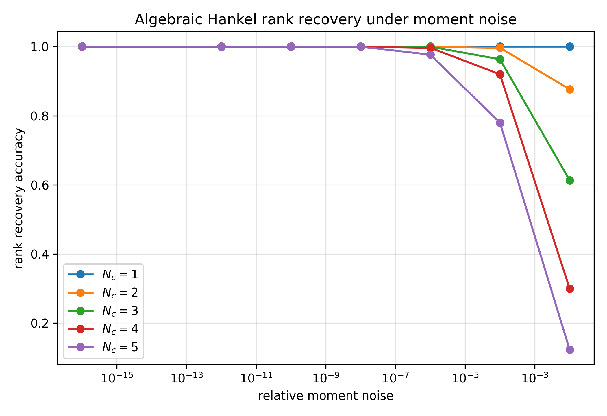
Table 1 reports the recovery accuracy. The rank is recovered exactly for all tested component numbers when the relative moment noise is at most \(10^{-8}\). At higher noise levels, the recovery accuracy decreases, and the degradation becomes more pronounced as \(N_{\rm c}\) increases. This behavior is consistent with the singular-gap condition in Theorem 2: larger values of \(N_{\rm c}\) generally lead to more ill-conditioned Vandermonde factors and smaller rank-revealing gaps.
| \(N_{\rm c}\) | \(0\) | \(10^{-12}\) | \(10^{-10}\) | \(10^{-8}\) | \(10^{-6}\) | \(10^{-4}\) | \(10^{-2}\) |
|---|---|---|---|---|---|---|---|
| 1 | 1.000 | 1.000 | 1.000 | 1.000 | 1.000 | 1.000 | 1.000 |
| 2 | 1.000 | 1.000 | 1.000 | 1.000 | 1.000 | 0.997 | 0.877 |
| 3 | 1.000 | 1.000 | 1.000 | 1.000 | 1.000 | 0.963 | 0.613 |
| 4 | 1.000 | 1.000 | 1.000 | 1.000 | 0.997 | 0.920 | 0.300 |
| 5 | 1.000 | 1.000 | 1.000 | 1.000 | 0.977 | 0.780 | 0.123 |
Figure 1 gives the same information graphically. The curves show a clear noise-dependent transition: the algebraic rank structure is robust under small perturbations, while high-order cases become more sensitive once the noise level approaches the singular gap.
The heatmap in Figure 2 further illustrates the same phenomenon. The stable region covers all tested values of \(N_{\rm c}\) at low noise, while the failure region first appears for larger \(N_{\rm c}\) and larger noise. This agrees with the theoretical dependence on the smallest nonzero singular value of the ideal Hankel matrix.

Finally, Figure 3 shows representative normalized singular values for the case \(N_{\rm c}=3\). In the noiseless case, the first three singular values are nonzero and the remaining singular values are at machine precision. As noise increases, the tail singular values are lifted, but the gap between \(\sigma_3\) and \(\sigma_4\) remains visible until the noise level becomes large. This is precisely the rank-revealing structure used by the estimator.

5.2 Experiment 2: Fourier–Hankel counting from Born far-field data↩︎
The previous experiment verified the algebraic Hankel rank mechanism directly on finite exponential moment sequences. In this experiment, we test the same mechanism on synthetic Born far-field data. The purpose is to examine whether the scaled row moment construction remains effective when the moments are not given explicitly but are computed from angular Fourier coefficients of the far-field pattern.
We generate scatterers consisting of \(N_{\rm c}=1,2,3,4\) separated localized components. For each configuration, the Born far-field data are computed from \[\begin{align} u^\infty(\hat{x},d;k) = C_k\int_D q(y)e^{-\mathrm{i}k(\hat{x}-d)\cdot y}\,\mathrm{d}y . \end{align}\] The empirical row coefficients \(a_{p0}^{\rm emp}(k)\) are obtained from the full-aperture angular data, and the scaled row moments are formed as \[\begin{align} \widehat b_p^{\rm row}(k) = \frac{p!}{C_k(-\mathrm{i})^p} \left(\frac{2}{k}\right)^p a_{p0}^{\rm emp}(k), \qquad p=0,1,\ldots,2J-2 . \end{align}\] The Hankel matrix \[\begin{align} \widehat H_J^{\rm row}(k) = \big(\widehat b_{r+s}^{\rm row}(k)\big)_{r,s=0}^{J-1} \end{align}\] is then constructed. We estimate the component number by the threshold rank \[\begin{align} \widehat{N_{\rm c}} = \#\left\{ \ell: \frac{\sigma_\ell(\widehat H_J^{\rm row})}{\sigma_1(\widehat H_J^{\rm row})} > \tau_{\rm rel} \right\}, \label{eq:exp295threshold95rank} \end{align}\tag{76}\] where \(\tau_{\rm rel}\) is a fixed relative singular-value threshold. For comparison, we also record the count obtained from a largest-gap rule applied to the normalized singular values. The latter is used only as a numerical benchmark; the theoretical stability result in Theorem 2 corresponds to the threshold-rank mechanism.
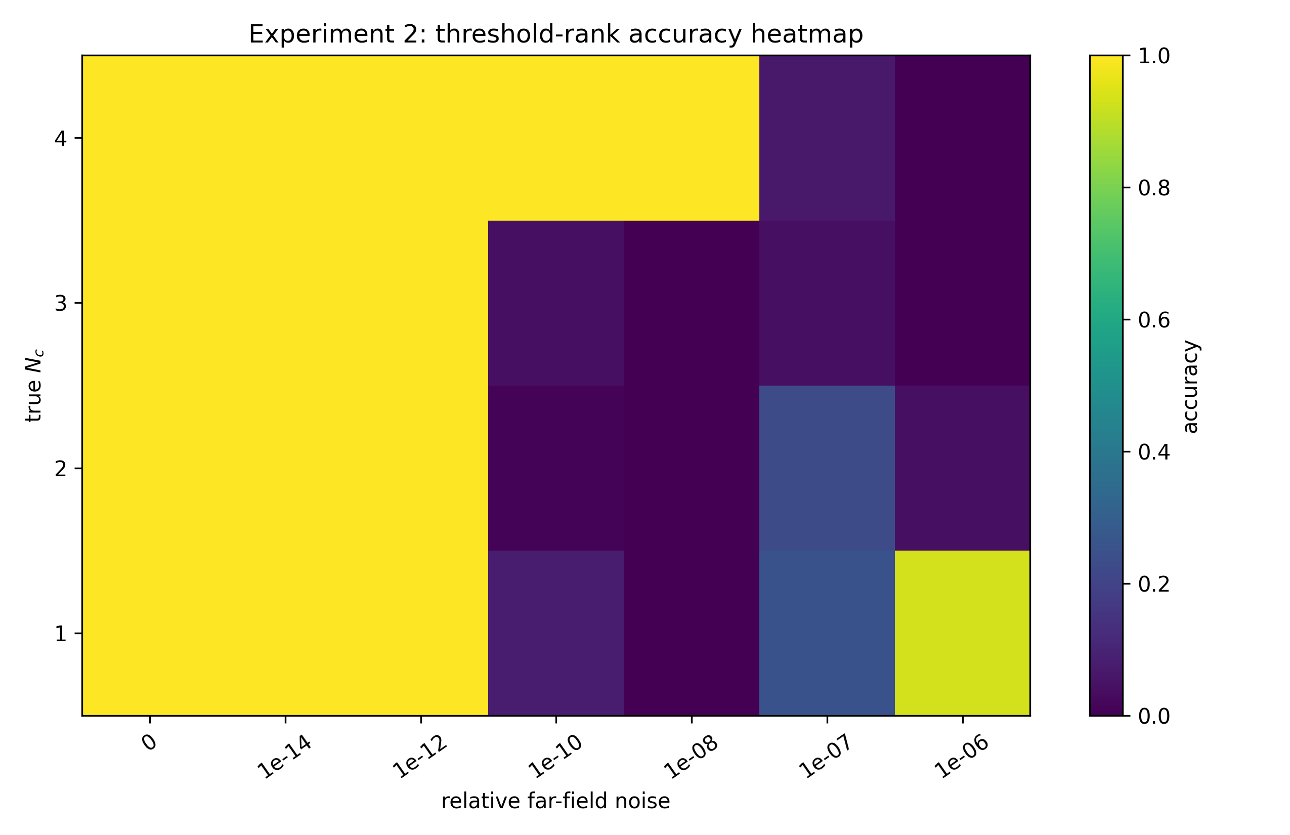
Figure 4 reports the component-counting accuracy over different true values of \(N_{\rm c}\) and different relative far-field noise levels. The Fourier–Hankel estimator accurately recovers the component number in the low-noise regime. In particular, for exact data and for sufficiently small far-field perturbations, the recovered rank agrees with the true value of \(N_{\rm c}\). When the far-field noise becomes larger, the accuracy deteriorates. This is consistent with the stability condition in Theorem 2: after Bessel leading-order scaling, perturbations in the raw Fourier coefficients are amplified by the factor \(p!(2/k)^p\), and the rank can no longer be separated once the induced Hankel perturbation is comparable with the singular gap.
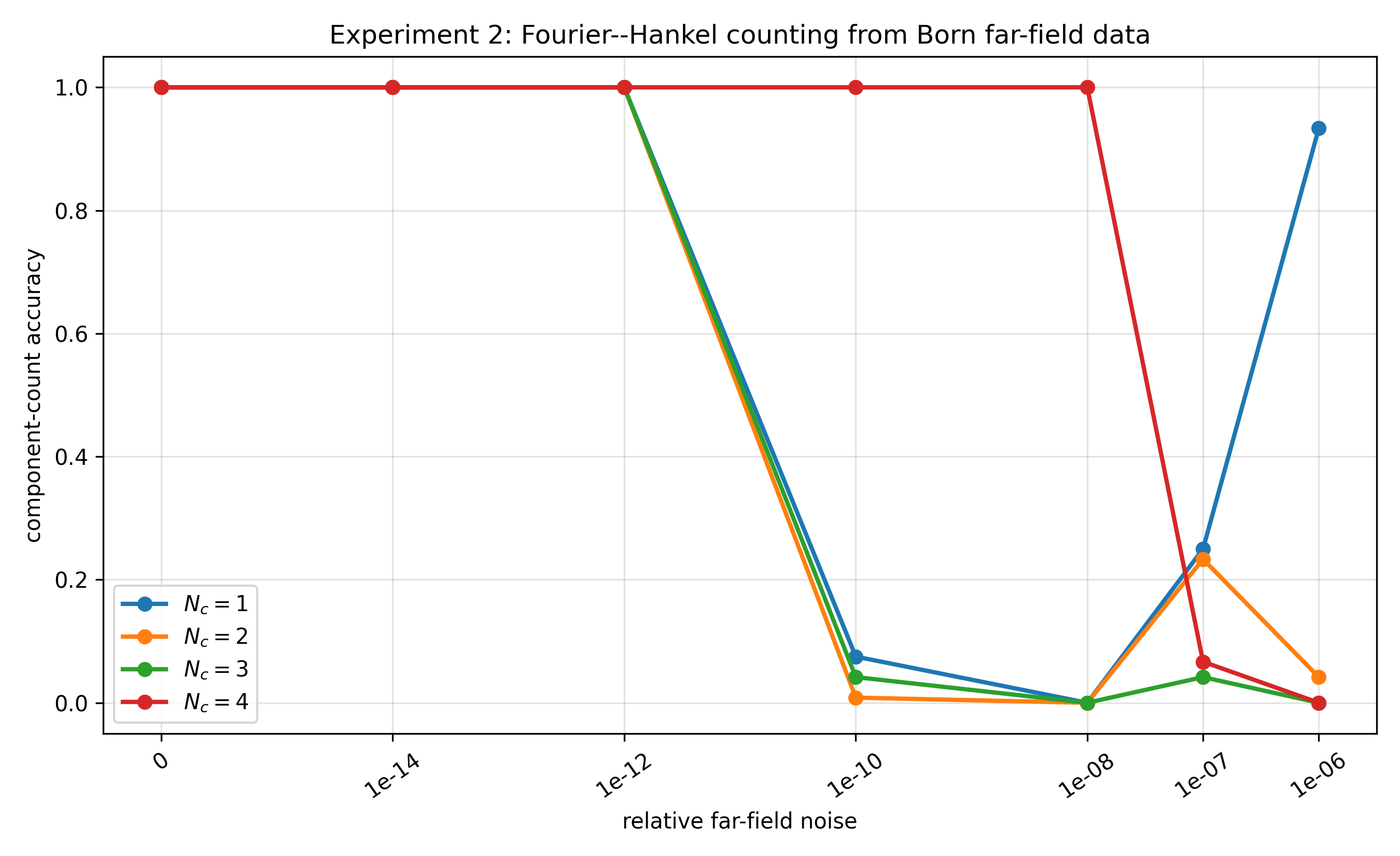
The same phenomenon is displayed in Figure 5, where the accuracy is plotted as a function of the relative far-field noise level for each \(N_{\rm c}\). The curves show a clear transition from the stable counting regime to the unstable regime. The high-noise behavior should not be interpreted as a reliable recovery phenomenon, since in that regime the numerical rank estimator may become dominated by noise-induced singular values or may collapse to a low-rank output.
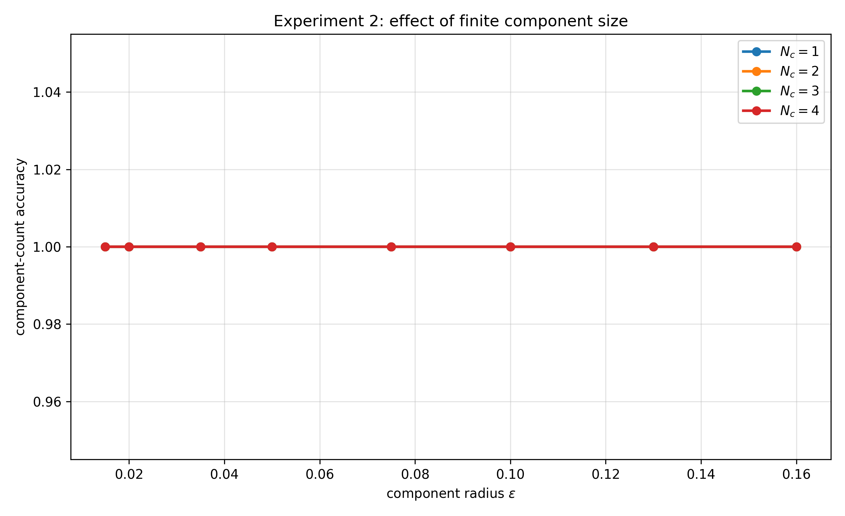
We next examine the effect of finite component size. The exact rank theorem is derived from the localized phase-center model, where each component is represented by one dominant phase center. For components of positive radius, finite-size effects generate residual terms beyond the leading exponential moment sequence. Figure 6 shows the counting accuracy as the component radius \(\varepsilon\) varies. In the tested range, the threshold-rank estimator remains accurate. This indicates that, for these configurations, the finite-size residual is still smaller than the relevant Hankel singular gap. Thus the phase-center approximation is sufficiently accurate for stable component counting in this regime.
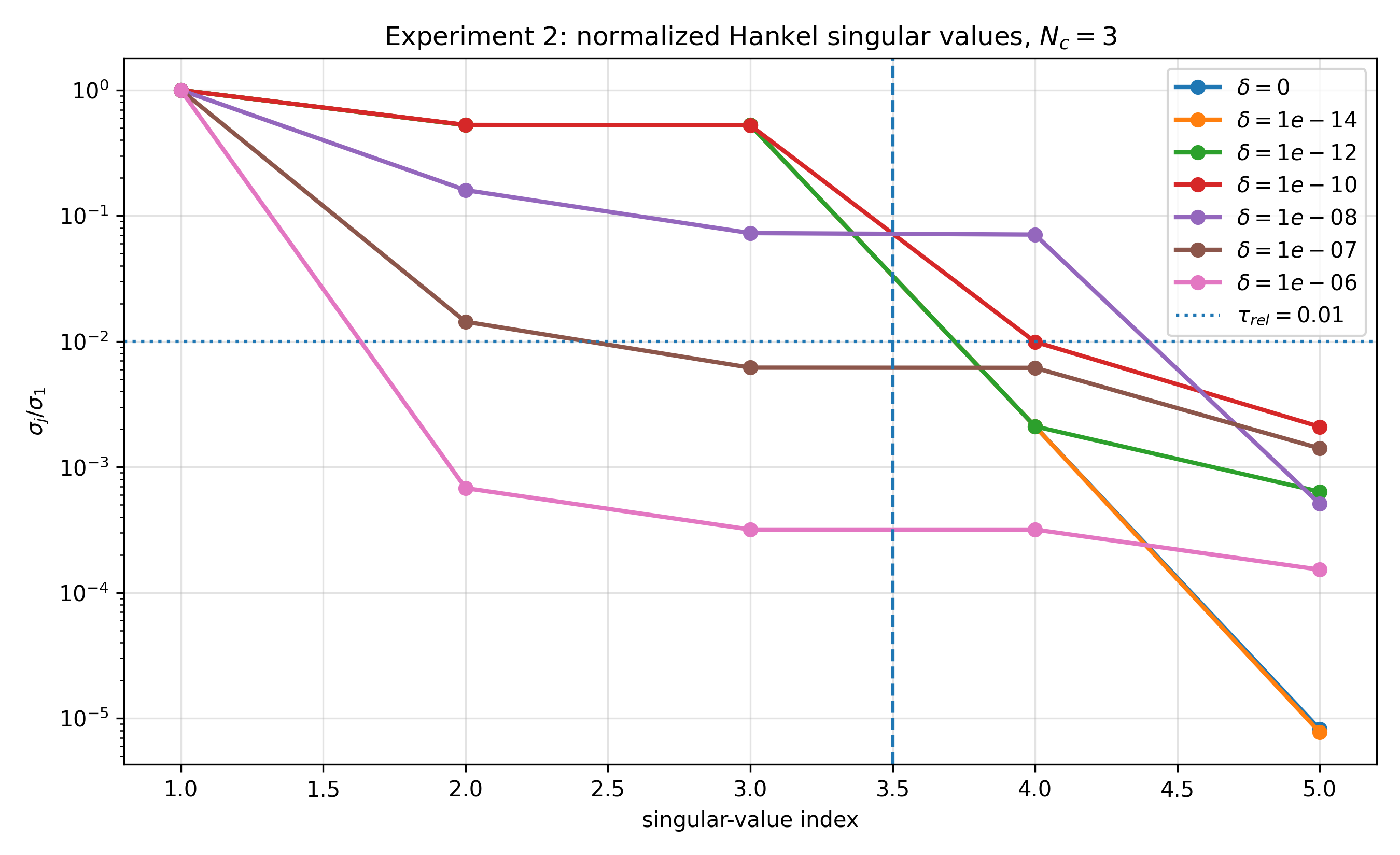
To explain the rank recovery more directly, Figure 7 plots representative normalized singular values of the Hankel matrix for the case \(N_{\rm c}=3\). In the exact or low-noise regime, the first three singular values are separated from the remaining singular values, producing a visible rank gap after index \(3\). As the far-field noise increases, the tail singular values are lifted, and the gap becomes less distinguishable. This confirms the mechanism behind Theorem 2: the component number can be recovered when the perturbation does not close the gap between \(\sigma_{N_{\rm c}}\) and the noise-dominated tail.
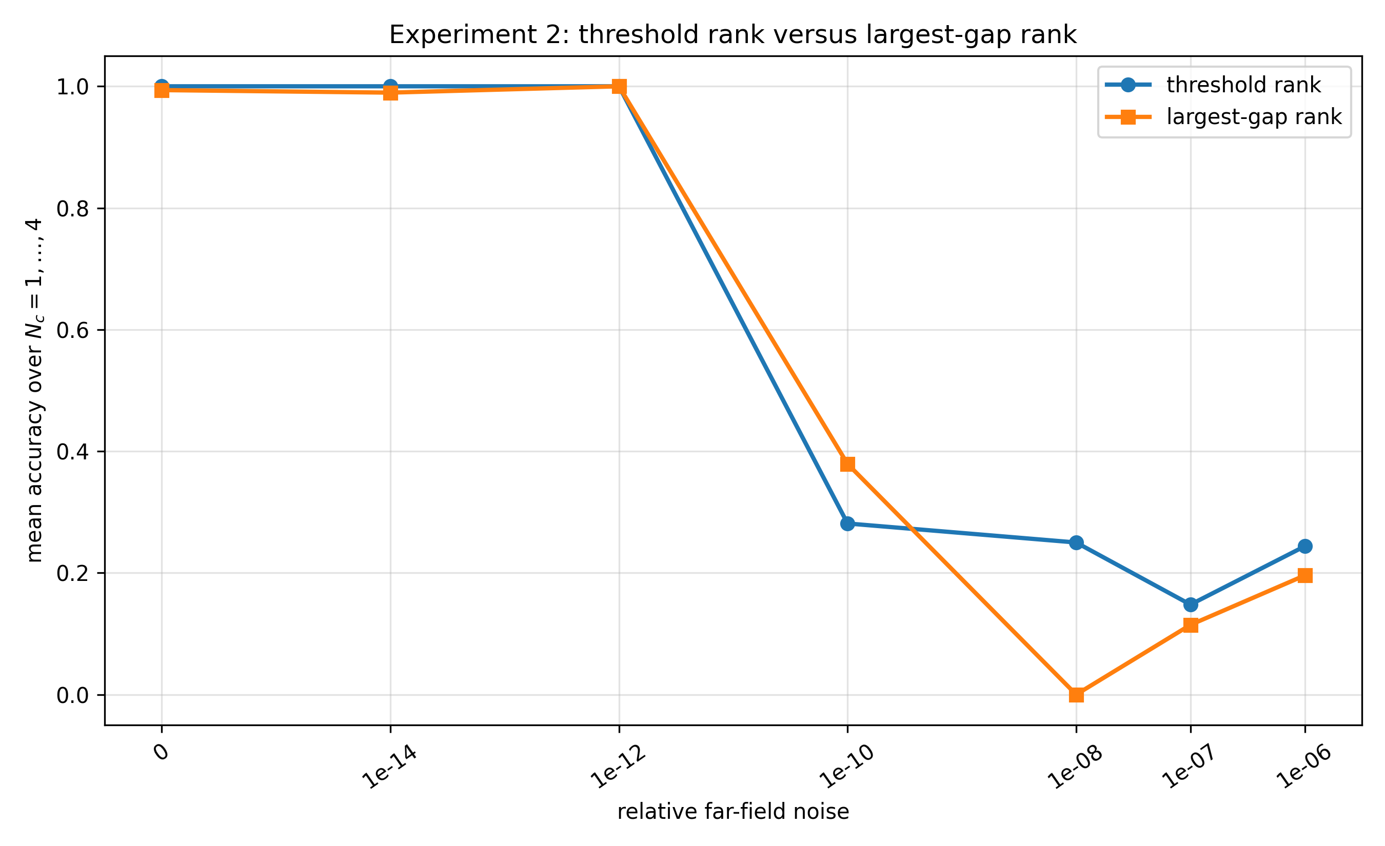
Finally, Figure 8 compares the threshold-rank rule with a largest-gap rule. The threshold-rank rule is directly tied to the perturbation theorem, because it counts the singular values above a prescribed noise-tolerance level. The largest-gap rule is more heuristic: it can work when the singular values have a pronounced spectral gap, but it may be less stable when the tail singular values are gradually lifted by noise or when the leading singular values decay unevenly. The comparison supports the use of the threshold-rank estimator as the default Fourier–Hankel counting rule.
Overall, Experiment 2 confirms that the Fourier–Hankel moment construction remains effective beyond the ideal algebraic moment setting. For synthetic Born far-field data, the method recovers the number of localized connected components whenever the finite-size residual and the scaled far-field noise are small relative to the Hankel singular gap. The observed failure at larger noise levels is therefore not a contradiction of the rank formula, but a manifestation of the perturbation bound and the noise amplification caused by the Bessel leading-order scaling.
5.3 Experiment 3: recovery of phase-center locations↩︎
The preceding experiments verify the use of the Fourier–Hankel matrix for component counting. We next test whether the same moment structure can also recover the component phase-center locations. This experiment is designed to support Corollary 1. In the ideal phase-center model, once the number of components \(N_{\rm c}\) is known, the phase nodes \(\lambda_j\) are recovered from a Hankel pencil or, equivalently, from a Prony annihilating polynomial. The physical phase-center locations are then given by \[\begin{align} z_j=(\operatorname{Re}\lambda_j,-\operatorname{Im}\lambda_j), \qquad j=1,\ldots,N_{\rm c}. \end{align}\]
We generated synthetic Born far-field data for scatterers consisting of \(N_{\rm c}=1,2,3,4\) small disk components. The component centers were randomly sampled in a bounded square subject to a minimum separation condition. For each configuration, the row Fourier coefficients \(a_{p0}\) were computed from full-aperture far-field data, the scaled Fourier–Hankel moments were formed, and the phase nodes were recovered by a Prony linear-prediction system. The estimated centers were matched to the true centers by the Hungarian assignment algorithm. A trial was counted as successful if the maximum matched center error was below a prescribed tolerance \(\varepsilon_{\rm loc}=0.08\).
Figure 9 reports the location-recovery success rate under different far-field noise levels. The method is accurate in the low-noise regime. For \(N_{\rm c}=1\) and \(N_{\rm c}=2\), the success rate remains essentially one over the tested noise range. For \(N_{\rm c}=3\), the recovery remains stable up to moderate noise and starts to deteriorate only at higher noise levels. For \(N_{\rm c}=4\), the method is still reliable for very small noise, but the success rate drops rapidly once the noise level reaches the range where the Prony root recovery becomes ill-conditioned.
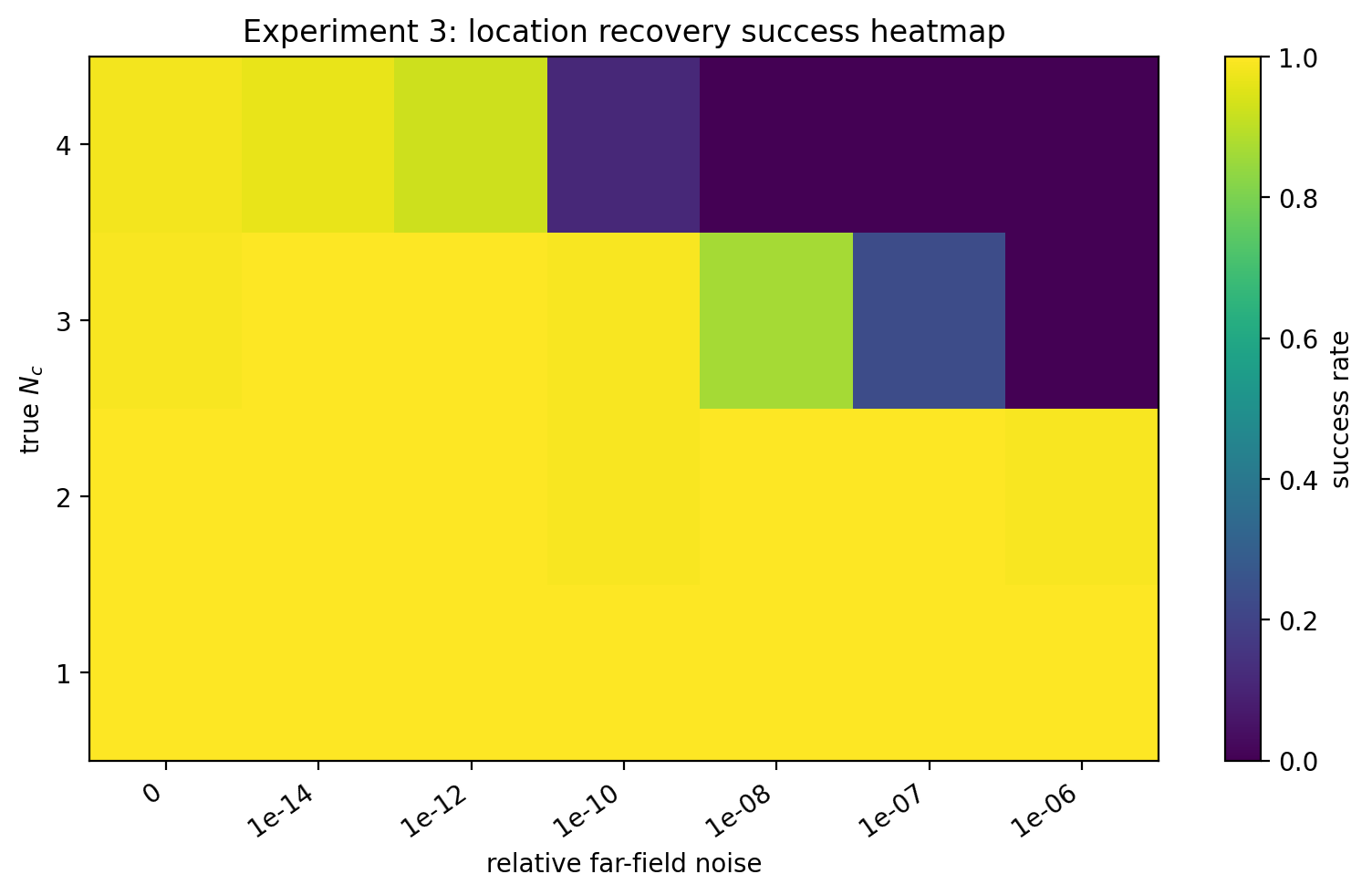
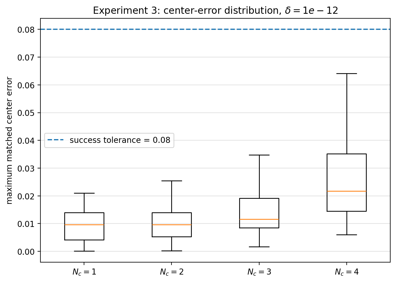
Figure 10 shows the distribution of the maximum matched center error at a representative low-noise level \(\delta=10^{-12}\). All tested component numbers have errors well below the success tolerance. The spread increases with \(N_{\rm c}\), which is consistent with the increasing ill-conditioning of the Vandermonde and Prony systems as more phase nodes are recovered from a fixed number of low-order moments.
A representative recovery result for \(N_{\rm c}=4\) is shown in Figure 11. The recovered phase centers closely match the true component centers. This confirms that the Fourier–Hankel moments contain not only counting information but also quantitative geometric information about the locations of the dominant phase centers.
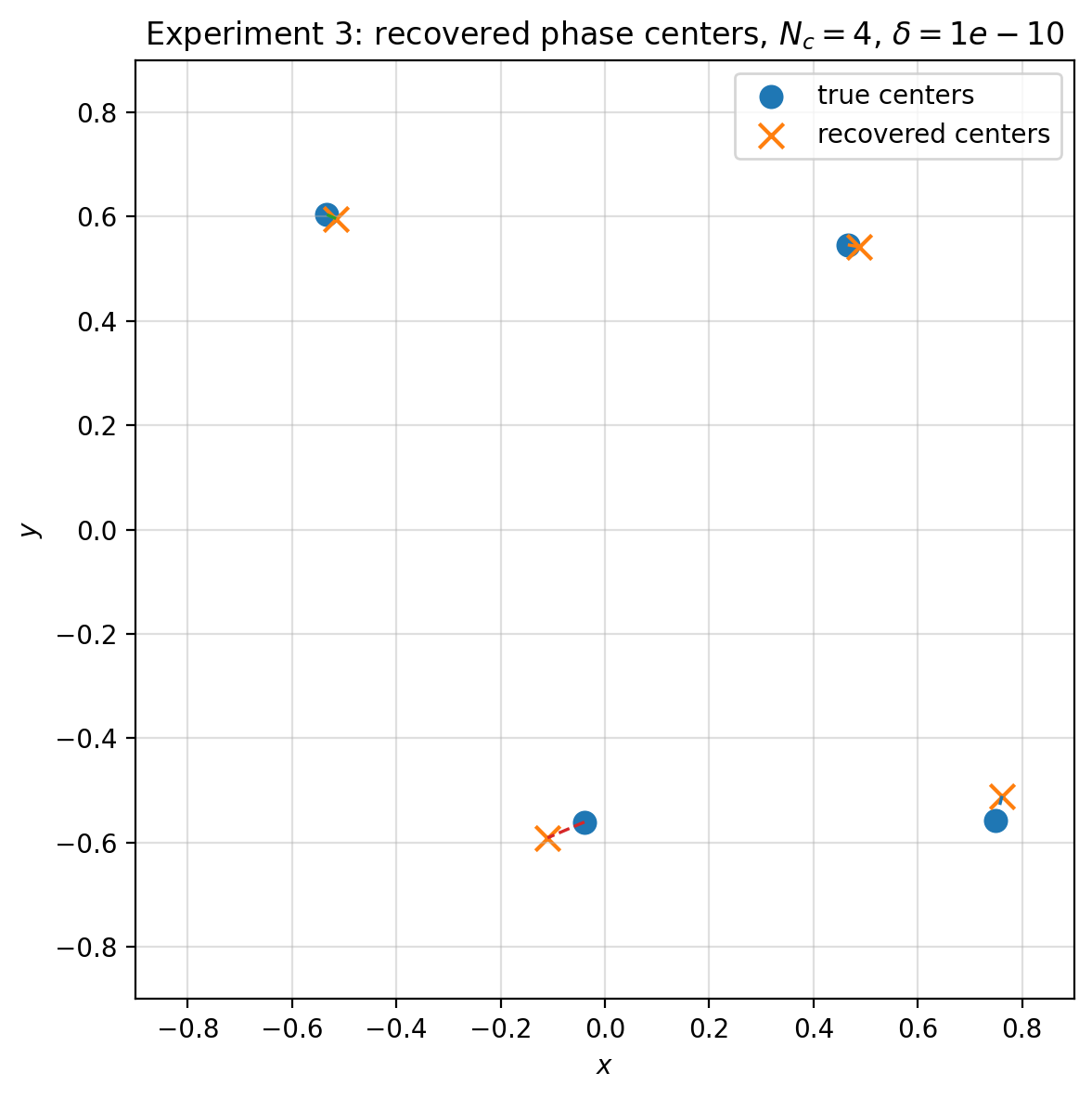
These results also reveal a limitation. Phase-center recovery is more sensitive to noise than rank-based component counting. The rank test only requires separation between the significant and insignificant singular values of the Hankel matrix, whereas location recovery requires solving a nonlinear root-finding problem for the Prony polynomial. Consequently, once the moment perturbation becomes comparable to the singular gap, a small perturbation may produce large errors in the recovered roots. This explains the rapid performance degradation for larger \(N_{\rm c}\) and higher noise levels.
5.4 Experiment 4: signed phase-center counting of cavities↩︎
This experiment tests the signed phase-center mechanism for cavity counting. According to the signed model, a material component contributes a positive phase-center term, while a cavity contributes a negative phase-center term. Thus the signed moment sequence has the form \[\begin{align} b_p^{\rm sgn} = \sum_{j=1}^{N_+}\alpha_j \lambda_j^p - \sum_{\ell=1}^{N_-}\beta_\ell \mu_\ell^p, \qquad p=0,1,\ldots,2J-2. \end{align}\] If all positive and negative phase nodes are distinct and all signed weights are nonzero, the signed Hankel rank is \[\begin{align} N_{\rm s}=N_+ + N_-. \end{align}\] When the number of connected components \(N_{\rm c}=N_+\) is known or estimated from the positive component-counting step, the detectable cavity number is estimated by \[\begin{align} \widehat h = \widehat N_{\rm s} - \widehat N_{\rm c}. \end{align}\]
We consider seven representative configurations: a disk without a hole, an off-center annulus, one component with two off-center holes, one component with three off-center holes, two components with two holes, a concentric annulus, and a nearly concentric annulus. The concentric annulus is included as a degenerate case, because the positive material phase center and the negative cavity phase center coincide in the leading signed phase-center model. In this case the signed rank does not increase, even though the physical domain contains a hole.
For each configuration, we generate the exact signed moment sequence and add relative complex moment noise with levels \[\delta\in \{0,10^{-14},10^{-12},10^{-10},10^{-8},10^{-7},10^{-6},10^{-5}\}.\] For each noise level, 400 independent trials are performed. The signed rank is estimated from the singular values of the signed Hankel matrix using a noise-aware relative threshold. We report two accuracies. The first is the physical hole-count accuracy, which compares \(\widehat h\) with the true geometric number of holes. The second is the detectable signed-rank accuracy, which compares \(\widehat h\) with the number of holes detectable by distinct signed phase nodes.
Figure 12 shows the detectable signed-rank hole-count accuracy. The method recovers the detectable cavity count almost perfectly for all tested configurations and all moderate noise levels. The only visible failure occurs for the three-hole configuration at the largest noise level \(\delta=10^{-5}\), where the weakest signed singular gap is lost.
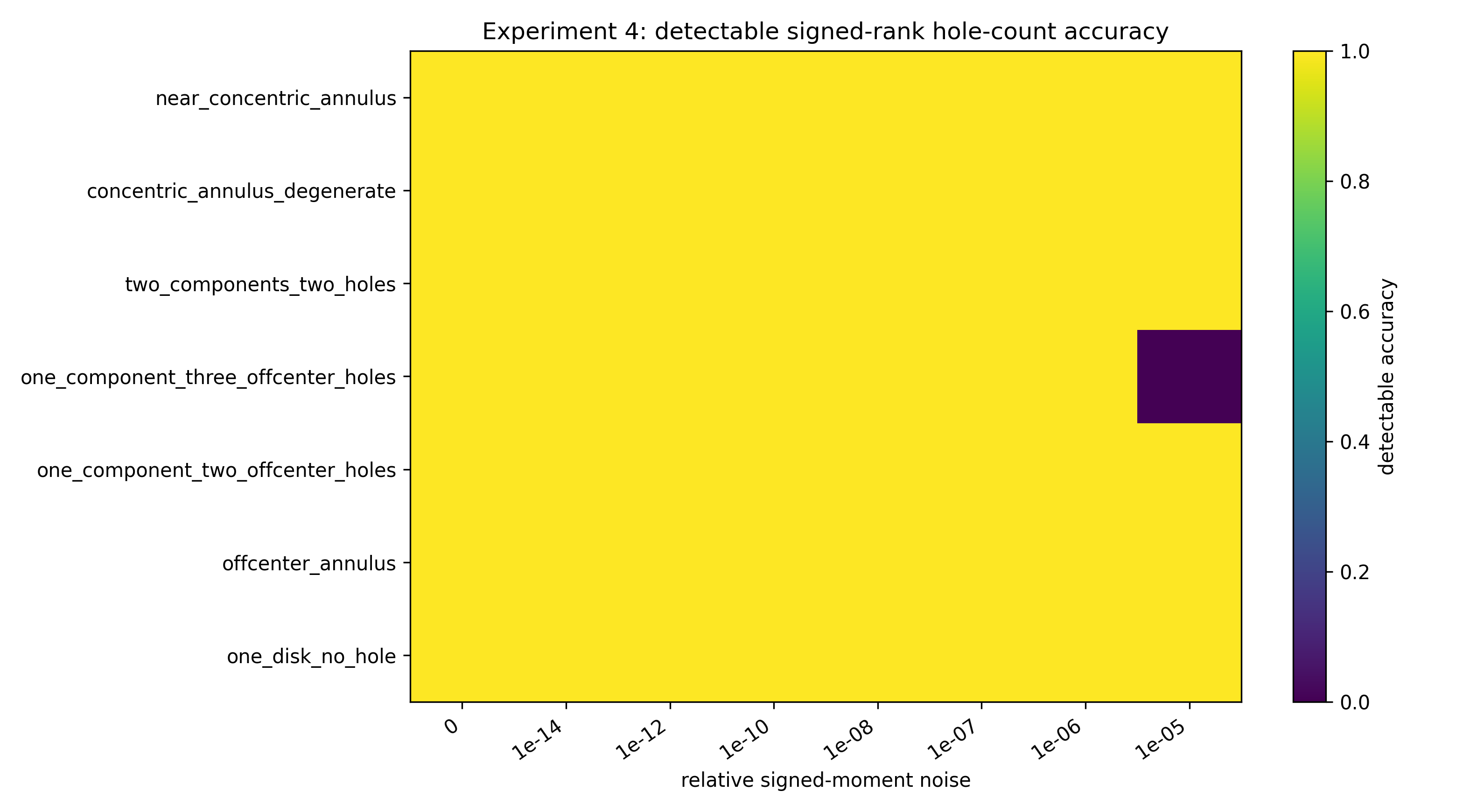
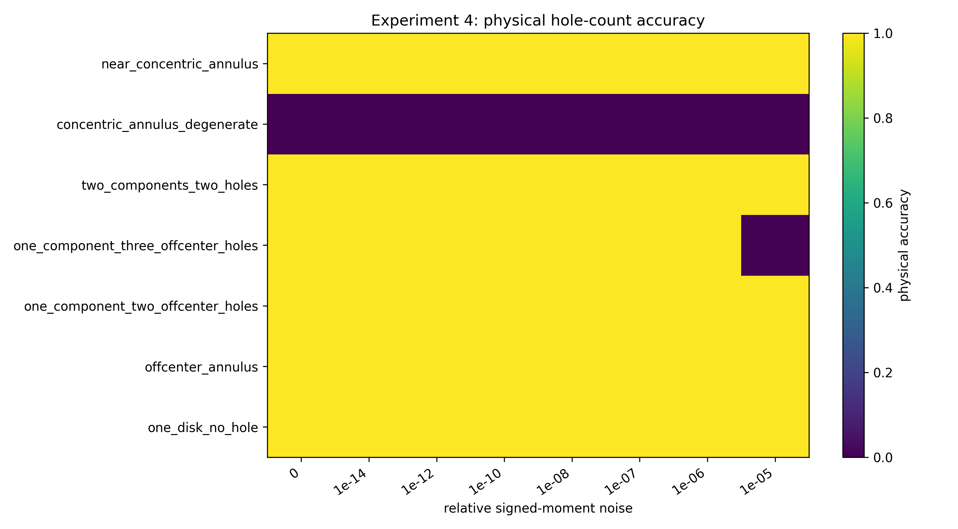
Figure 13 reports the physical hole-count accuracy. The result is identical to the detectable accuracy for all nondegenerate cases. The only systematic discrepancy occurs for the concentric annulus. This is expected: the physical domain has one hole, but the positive and negative phase centers coincide, so the leading signed phase-center model has only one detectable node. Hence the signed Hankel rank cannot distinguish a perfectly concentric annulus from a disk with modified signed strength.
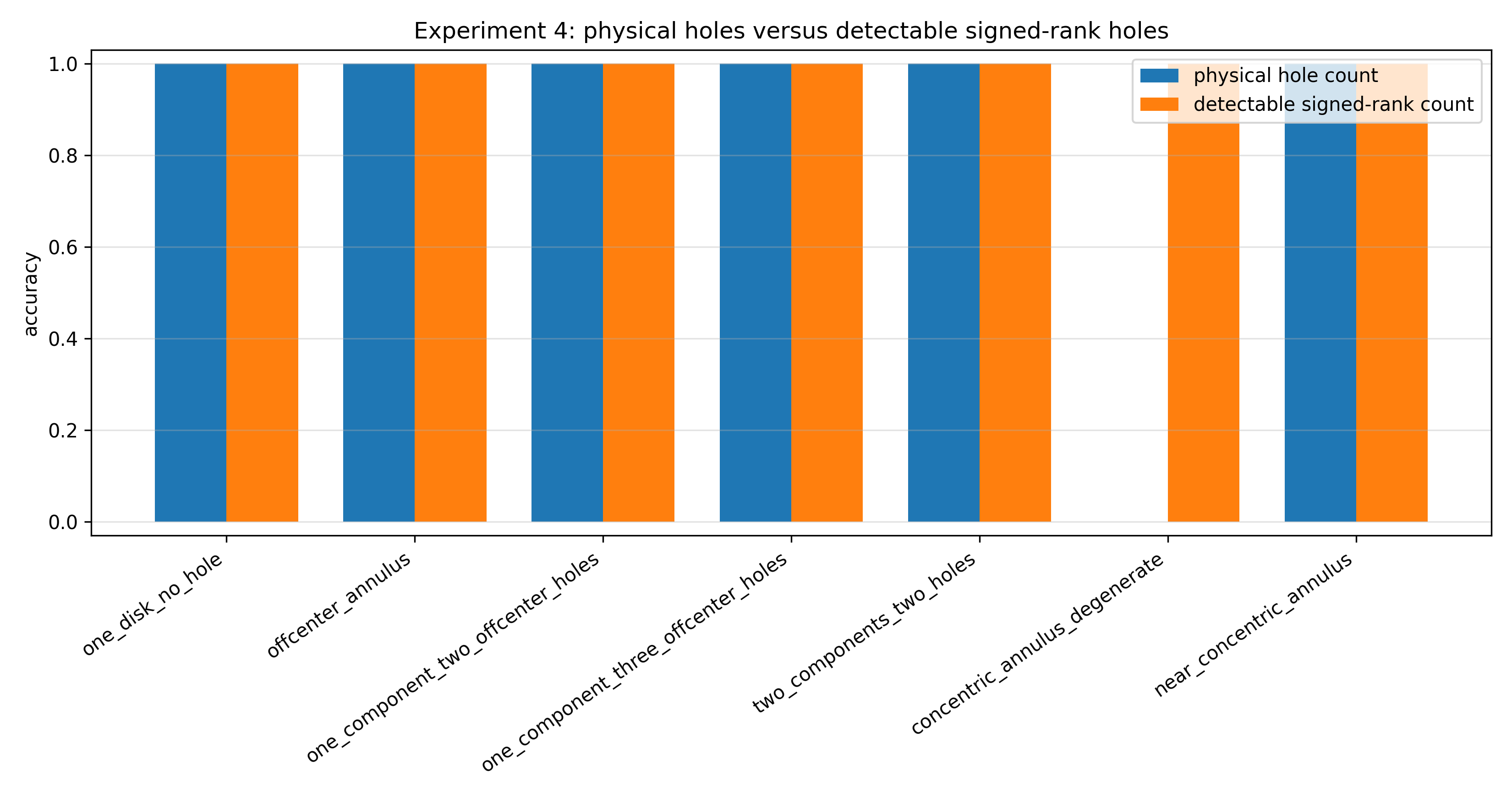
The distinction between physical and detectable cavities is summarized in Figure 14. For the concentric annulus, the physical hole-count accuracy is zero, whereas the detectable signed-rank accuracy is one. This confirms that the failure is not numerical instability but a structural degeneracy of the leading signed phase-center representation.
Finally, Figure 15 displays representative normalized singular values of the signed Hankel matrices. The nondegenerate off-center annulus and the two-hole case exhibit clear rank transitions corresponding to their signed phase-node counts. The concentric annulus has only one effective singular value, reflecting the collapse of the positive and negative nodes into a single signed node. The nearly concentric annulus remains detectable in the noise-free model, but its stability depends on the singular gap and is therefore more sensitive to perturbations when the positive and negative phase centers become closer.
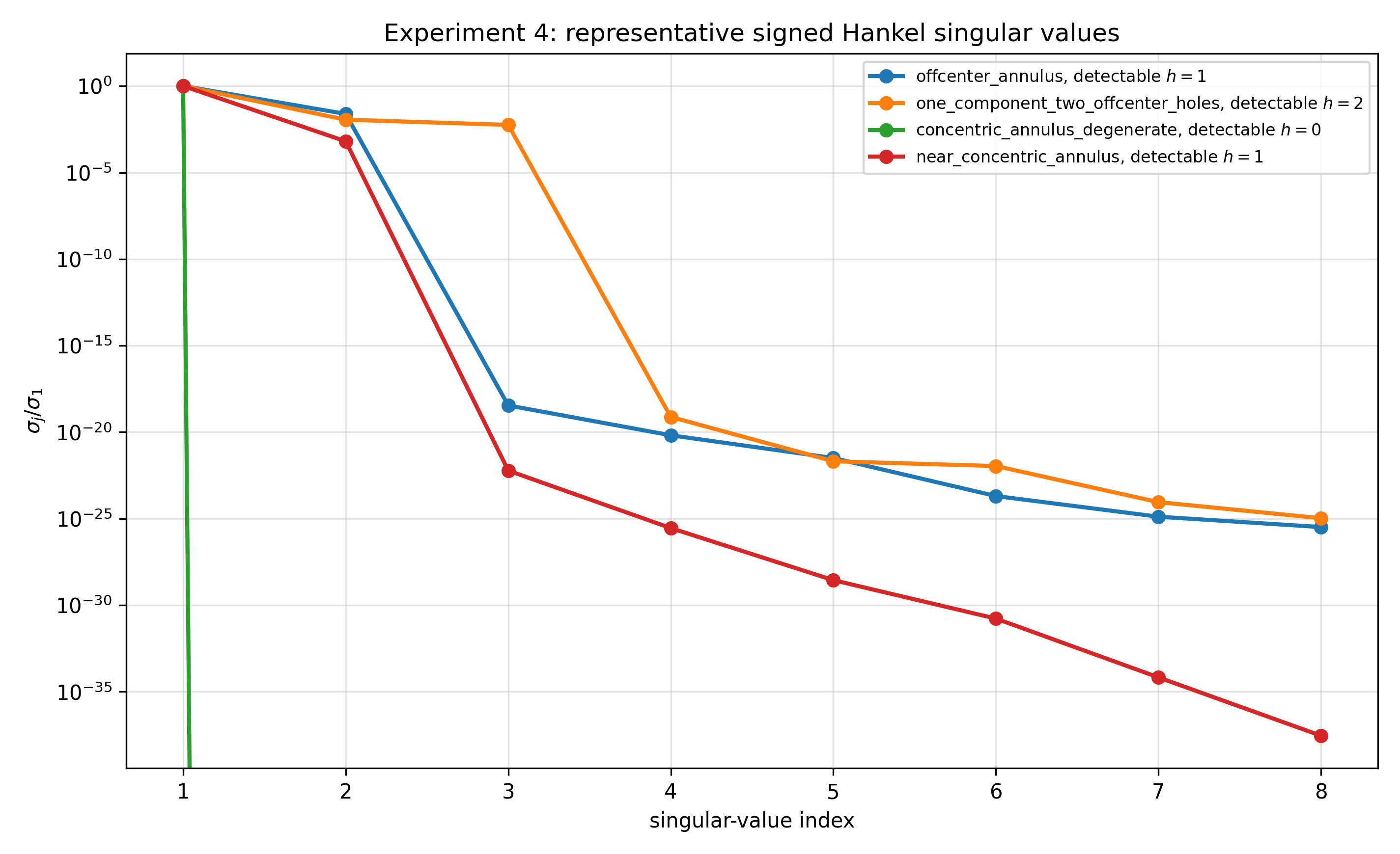
These results support the signed Fourier–Hankel interpretation of cavity counting. The method does not claim to detect every geometric hole unconditionally. Rather, it detects holes that generate distinct negative phase centers in the leading signed phase-center model. Degenerate cavities, such as perfectly concentric annuli, require additional radial information, higher-order Fourier–Bessel channels, or multiple frequencies.
5.5 Exact Helmholtz validation beyond the Born model↩︎
The preceding experiments were based on algebraic moments or Born-type far-field data. We now test whether the Fourier–Hankel rank mechanism remains observable for exact Helmholtz scattering data. To this end, we consider multiple sound-soft circular obstacles in two dimensions and compute the full-aperture multistatic far-field matrix by a multipole expansion. The data therefore include finite-size effects and multiple scattering between different components, and are no longer generated by the ideal phase-center model.
For each value of \(N_c=1,2,3,4\), we generate \(N_c\) well-separated sound-soft disks of radius \(0.04\). The wave number is fixed at \(k=1.6\). The far-field matrix is sampled on a uniform \(96\times96\) grid of observation and incident directions. From the computed far-field matrix we form the row Fourier–Hankel moments and construct a \(5\times5\) Hankel matrix. The component number is estimated by the relative threshold rule \[\widehat N_c = \#\{j:\sigma_j(\widehat H_J)/\sigma_1(\widehat H_J)>\tau_{\rm rel}\}, \qquad \tau_{\rm rel}=10^{-2}.\] Complex Gaussian noise is added to the far-field matrix at relative levels \[\delta=0,10^{-14},10^{-12},10^{-10},10^{-8},10^{-7},10^{-6},10^{-5}.\] For each configuration and each noise level, the experiment is repeated over random rotations of the component configuration.
Figure 16 reports the component-counting accuracy. The threshold-rank estimator recovers the correct number of components with essentially perfect accuracy for all tested component numbers when \(\delta\le 10^{-6}\). Accuracy deteriorates only at the highest noise level \(\delta=10^{-5}\), where the noise floor begins to lift the small singular values above the fixed threshold. This confirms that the Fourier–Hankel rank signature is not merely an artifact of the Born approximation, but remains visible in exact Helmholtz scattering data for localized separated components.
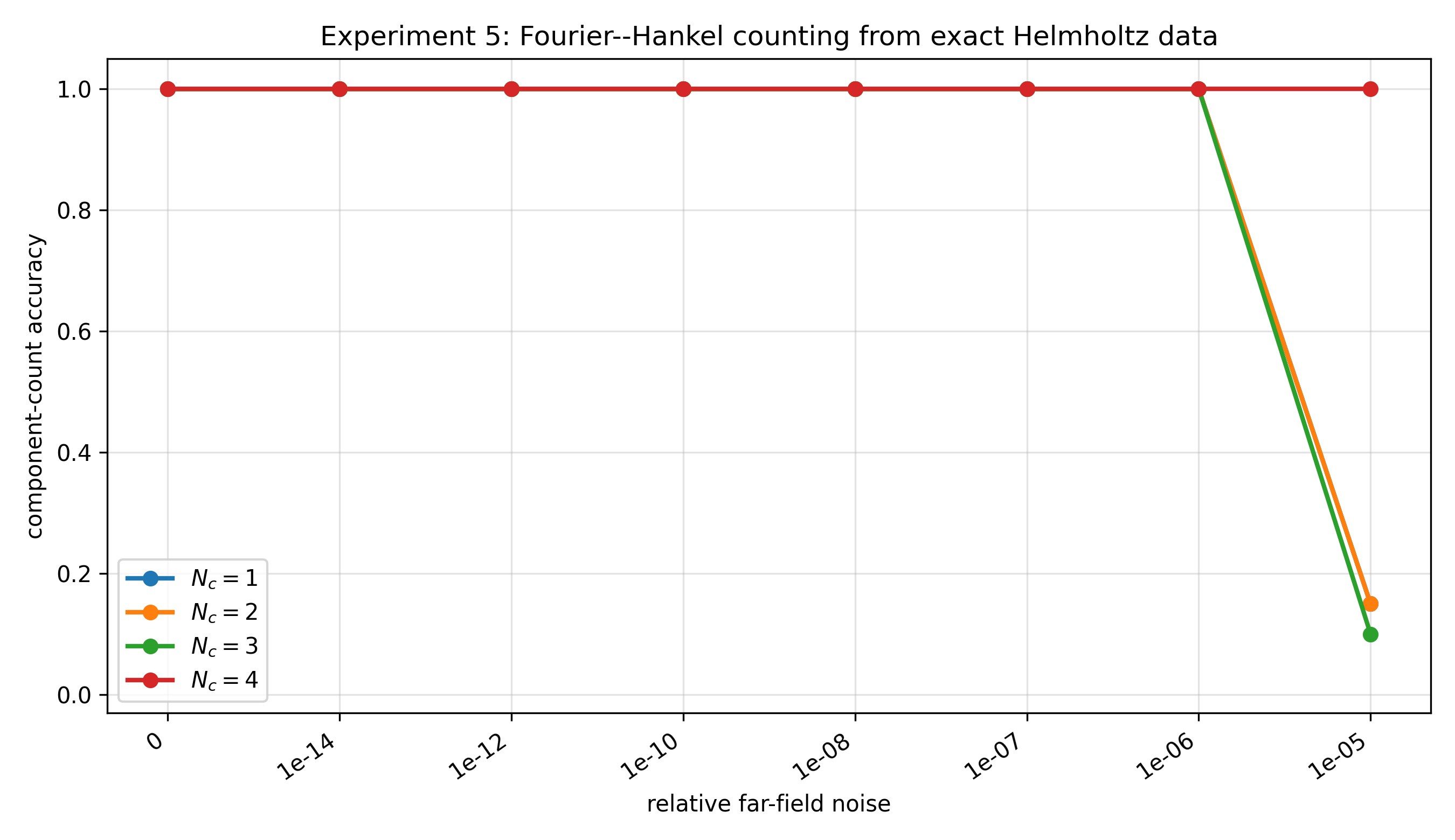
The corresponding accuracy heatmap in Figure 17 gives the same conclusion. For \(\delta\le 10^{-6}\), the method correctly recovers \(N_c=1,2,3,4\) in all trials. At \(\delta=10^{-5}\), the performance decreases for some smaller component counts, reflecting over-estimation caused by noise-amplified small singular values.

We also compare the fixed threshold-rank estimator with a largest-gap rank estimator. As shown in Figure 18, the threshold rule is more robust. The largest-gap estimator can select an incorrect gap, especially when the singular values decay gradually rather than exhibiting a single dominant jump. For this reason, the fixed relative threshold rule is used as the main counting rule in all subsequent experiments.

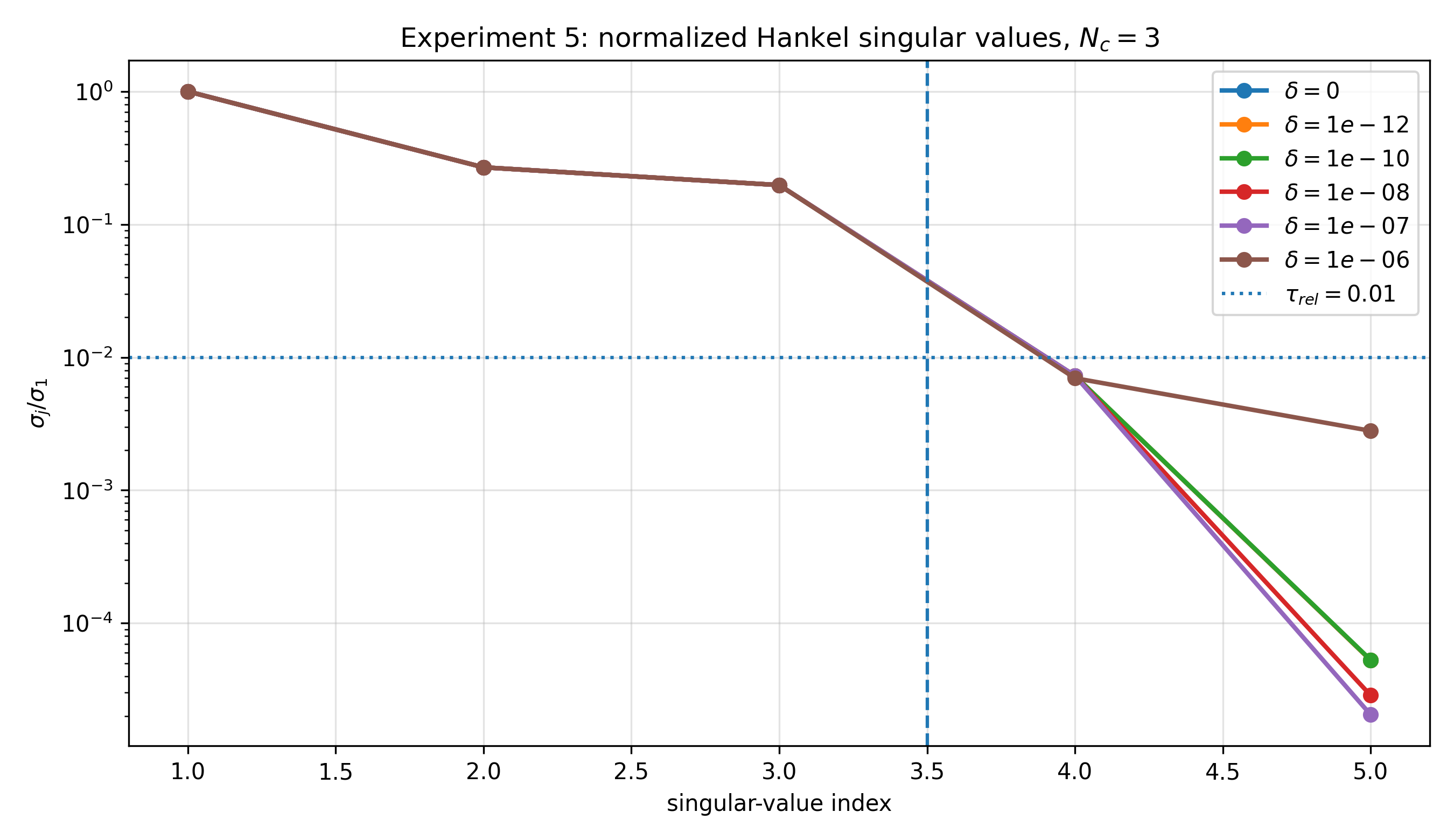
Finally, Figure 19 displays representative normalized singular values for the case \(N_c=3\). The first three singular values remain above the threshold \(\tau_{\rm rel}=10^{-2}\), whereas the fourth singular value lies below the threshold for noise levels up to approximately \(10^{-6}\). This clear spectral separation explains the observed stability of the rank estimator.
6 Conclusions↩︎
This paper developed a Fourier–Hankel moment framework for extracting topological counting information and phase-center locations from acoustic far-field data. The starting point is the angular spectral structure of the multistatic far-field pattern. Under the Born approximation, the Bessel–Fourier moment identity shows that the angular Fourier coefficients are moments of the weighted scattering support. For separated localized components, a Bessel leading-order scaling of the row moment channel yields, to leading order, a finite exponential moment sequence. The corresponding Hankel matrix admits a Vandermonde factorization, and its rank equals the number of separated phase centers. This gives an algebraic component-counting mechanism directly at the data level, rather than through thresholding a reconstructed image.
The exact Hankel rank formula was proved for the ideal phase-center moment sequence, and a perturbation result was established for empirical moments. The stability theorem shows that the numerical rank recovers the component count when the scaled moment perturbation is smaller than the singular gap of the ideal Hankel matrix. This condition also clarifies the main sources of instability: weak component strengths, nearly colliding phase nodes, Bessel-zero frequencies, finite-size residuals, discretization errors, measurement noise, and model mismatch beyond the Born phase-center model. The analysis further explains the frequency trade-off in the scaling: lower frequencies reduce the Bessel-modulation residual, but they also amplify high-order coefficient errors through the factor \(p!(2/k)^p\).
Beyond component counting, the same moment structure gives phase-center location recovery through a Hankel pencil. This provides a skeleton-type geometric reconstruction of the dominant scattering components. The paper also introduced a signed phase-center extension for cavity counting. In this model, material components and cavities contribute with opposite signs to the leading moment sequence. The signed Hankel rank counts distinct signed phase centers, and the excess over the positive component count gives the number of detectable cavity phase centers. This formulation identifies an intrinsic detectability limit: a physical cavity whose phase center coincides with a material phase center, as in a perfectly concentric annulus, does not increase the leading signed rank and therefore cannot be detected by this leading phase-center mechanism alone.
The numerical experiments support the theoretical conclusions. The algebraic rank mechanism was first verified on ideal exponential moment sequences. The method was then tested on Born far-field data with finite-size components and noise, where the observed behavior matched the singular-gap stability prediction. Phase-center location recovery was demonstrated through the Hankel-pencil procedure, while the signed phase-center experiments confirmed the distinction between physical cavities and detectable signed-rank cavities. Finally, simulations with exact Helmholtz far-field data for sound-soft disks showed that the Fourier–Hankel rank signature persists beyond the Born data-generation model for localized separated scatterers.
The proposed method should therefore be viewed as a data-level algebraic tool for topological counting and phase-center recovery. It is not intended to replace full shape reconstruction methods, nor does it claim unconditional recovery of all geometric cavities. Its strength lies in identifying rank-revealing moment structures that encode component and detectable cavity information directly from far-field data. One limitation remains intrinsic to the leading signed phase-center model. Degenerate cavities whose phase centers coincide with material phase centers do not generate additional signed phase nodes and therefore do not increase the signed Hankel rank. A perfectly concentric annulus is the canonical example: although it contains a physical cavity, its leading positive and negative phase-center contributions collapse into a single node. Detecting such cavities requires information beyond the leading phase-center term, for example higher-order radial Fourier–Bessel information or multi-frequency signatures. Understanding how to incorporate this additional radial information into a stable Hankel-type counting framework is a natural direction for future work.