No title
January 01, 1970
Abstract
Abstract. We present a new method together with a proof-of-concept implementation for determining the Landau singularities of Feynman integrals, read off directly from where the Euler characteristic of the associated integral drops. Working over finite fields makes the requisite elimination tractable for multi-scale integrals at the multi-loop frontier. The algorithm returns the genuine and complete set of singularities, subject to a set of conditions which are practically testable. We apply these methods to classes of Feynman integrals beyond the reach of current methods, including non-planar six-point diagrams at two loops, as well as a fully massive three-loop envelope graph. Several of the newly found singularities, both in \(d\)- and 4-dimensional external kinematics, are of unexpected complexity when compared to previously known singularities for these examples.
1 Introduction↩︎
Modern high-precision phenomenology at colliders and gravitational-wave observatories relies on our ability to compute scattering amplitudes to ever higher loop orders. A lesson of the past decade is that the difficulty of these computations is controlled, to a large extent, by our understanding of the analytic structure of the underlying Feynman integrals: the locations of branch points and discontinuities provide powerful constraints on their functional forms, often at much lower cost than head-on integration.
The locations of these branch points and discontinuities are not arbitrary. They arise where the integration contour is pinched between colliding singularities of the integrand, a mechanism that was recognised long ago [1]–[4]. Together, they form the set of Landau singularities (or simply the Landau locus) and delineate the boundary of analyticity of the integral.
However, for these data to be maximally useful, one would like to obtain them before committing to a full computation of the integrals, which grows prohibitively expensive with the number of loops and legs. A productive idea has been to invert the logic and leverage the Landau locus: once known, it provides input to the symbol alphabet, to integration-by-parts and differential-equation methods [5]–[9] as well as direct evaluation strategies [10], [11], and it seeds bootstrap and ansatz-based reconstructions of the individual Feynman integrals [12], [13] or even the amplitude itself [14]–[16].
Determining the Landau locus more systematically beyond one loop has only recently become feasible through several distinct frameworks. Building on the modern reformulation of [17], [18], the principal Landau determinant (PLD) recast the problem in computational algebraic geometry and made the extraction of the Landau locus practical for realistic multi-scale processes [19], [20]. A separate line extracts singularities from Whitney stratifications of the relevant varieties [21], [22]. The automated Mathematica program , working within yet another framework [10], [23], organises the analysis by sectors and, among the above, currently offers the broadest practical coverage of examples relevant, e.g., for precision Standard Model physics.
However, two limitations persist. First, all of these methods become computationally prohibitive on certain classes of graphs. For example, some multi-loop (near) maximally connected diagrams (e.g., [fig:new95applications]) lie beyond reach and represent a sharp class of bottleneck diagrams that mark the current computational frontier, where new and complementary methods are needed.
Second, many of these methods return a superset of the genuine Landau locus, whose spurious factors must be removed by hand, or, worse, a subset that misses genuine singularities altogether and is therefore incomplete for practical amplitude computations.
In this Letter we propose a route that addresses both issues simultaneously. The key object is a number known as the (absolute value of the) Euler characteristic \(\chi(\boldsymbol{s})\) associated to the Feynman integral, or more generally to any parametric (Euler) integral in Lee–Pomeransky form [24]. Physically, it counts the number of master integrals [24], [25], which in turn equals the number of critical points of the associated parametric integral [26].
Euler characteristics have been used extensively to test whether a candidate singularity is genuine [20]. In this work we turn this idea around and propose to use \(\chi\) to find the locus directly (see also [27]). In this picture, the Landau singularities are precisely the locations in kinematic space where \(\chi\) drops, i.e., where some critical points “escape” to a boundary of the parametric space.
Detecting where this happens is made efficient by working with finite field arithmetic, which renders the required algebra tractable even for the many-parameter systems generated by cutting-edge multi-loop and multi-scale Feynman integrals. In practice,
we use the package SP\(\mathbb{Q}\)R [28] for polynomial algebra, which leverages FiniteFlow
[29], [30] as its primary back end.
Because this method pinpoints the locus from the critical points that are genuinely lost, this approach returns the strict set of genuine singularities directly rather than a superset. The computational framework behind this construction is simple, and we accompany this Letter with a proof-of-concept Mathematica implementation showcasing its most important features.
For practical computational purposes, one often works “sector-by-sector”, which trades some mathematical rigour in exchange for computational speed. Nevertheless the full set of singularities can still be found in the vast majority of cases, subject to a set of conditions which are practically testable.
After describing the construction in detail, we put the method to the test on two bottleneck families beyond the reach of existing tools: the two hardest non-planar six-point diagrams at two loops, as well as the fully massive four-scale three-loop non-planar envelope, all shown in [fig:new95applications]. The resulting singularity lists and our proof-of-concept Mathematica implementation are collected in the GitHub repository .
2 Method↩︎
Euler Characteristics.Our strategy for locating the singularities of Feynman integrals revolves around computing the Euler characteristic \(\chi(\boldsymbol{s})\) as a function of kinematic variables \(\boldsymbol{s}\). To this end, we consider a Feynman integral with \(E\) internal edges in Lee–Pomeransky [24] representation in \(d\) spacetime dimensions \[\require{physics} \label{eq:reg95I} I_{\boldsymbol{\nu}}(\boldsymbol{s}) \propto \int_0^\infty \boldsymbol{x}^{\boldsymbol{\nu}} \mathcal{G}(\boldsymbol{x},\boldsymbol{s})^{-d/2} \frac{\dd\boldsymbol{x}}{\boldsymbol{x}}\qquad (\boldsymbol{\nu},d)\in\mathbb{C}^{E+1}\,.\tag{1}\] Here, \(\boldsymbol{x}^{\boldsymbol{\nu}}\equiv x_1^{\nu_1}\ldots x_E^{\nu_E}\) and an irrelevant, kinematically independent prefactor has been omitted from our discussion. Although we focus on Lee–Pomeransky representation for this work, the method can be applied to other parametric representations, such as standard Baikov [31]–[33], as well as the broader class of Euler integrals, for example see the review [34]. Up to an overall irrelevant sign, \(\chi(\boldsymbol{s})\) is computed as \[\label{eq:chi1}\chi(\boldsymbol{s}) = \# \text{ of solutions to} \,\, \mathrm{d}\log\bigl(\boldsymbol{x}^{\boldsymbol{\nu}}\mathcal{G}^{-d/2}(\boldsymbol{x},\boldsymbol{s})\bigr) = 0\,.\tag{2}\] Physically, \(\chi(\boldsymbol{s})\) counts the number of master integrals of the regulated Feynman integral family \(I_{\boldsymbol{\nu}}(\boldsymbol{s})\) [35]. 2 is equivalent to the system of polynomial equations (referred to as an ideal), given by \[\label{eq:chi95ideal95reg}\mathcal{I}\equiv\left\langle \nu_1\mathcal{G}-\frac{d}{2}x_1 \partial_1\mathcal{G} ,{\ldots}, \nu_E \mathcal{G}-\frac{d}{2} x_E \partial_E\mathcal{G}, 1{-}x_0\boldsymbol{x} \mathcal{G} \right\rangle,\tag{3}\] where the final generator, together with the auxiliary variable \(x_0\), removes any solutions lying on the hypersurface \(x_1\cdots x_E\,\mathcal{G}=0\). Equivalently, \(\mathcal{I}\) describes the critical points on the variety \(X_{\boldsymbol{s}}=(\mathbb{C}^*)^E\setminus\{\mathcal{G}=0\}\), whose boundary components are \(\{x_i=0\}\cup\{x_i=\infty\}\cup\{\mathcal{G}=0\}\). For generic \((\boldsymbol{\nu},d)\) the ideal \(\mathcal{I}\) is always zero-dimensional [36], [37], so its solution set, denoted as \(V(\mathcal{I})\), consists of finitely many isolated critical points. The number (counted with multiplicity) of such points is known as the degree of the ideal \[\label{eq:ChiDeg} \chi(\boldsymbol{s}) = \deg(\mathcal{I}(\boldsymbol{s}))\equiv \text{Cardinality}(V(\mathcal{I}))\,.\tag{4}\]
For generic kinematics \(\boldsymbol{s}\), the value of \(\chi(\boldsymbol{s})\) is constant. On a special locus \(\boldsymbol{s}^*\), however, the Euler characteristic may drop discontinuously to a lower value [20], [22], [26]: \[\label{eq:euler95chi95drop} \chi(\boldsymbol{s}^*) < \chi(\boldsymbol{s}) \,.\tag{5}\] Since \(\chi\) is a topological invariant, such a drop signals a change in \(X_{\boldsymbol{s}}\)’s topology, occurring precisely where a new singularity develops at a point \(\boldsymbol{s}^*\) in kinematic space. These special locations are therefore in one-to-one correspondence with the branch points of \(I_{\boldsymbol{\nu}}(\boldsymbol{s})\): writing \(l(\boldsymbol{s})=l_1(\boldsymbol{s})\cdots l_N(\boldsymbol{s})\) for the product of all singularities of the Feynman integral, 5 holds precisely when \(l(\boldsymbol{s}^*)=0\). From now on, we will refer to these singularities of 1 as Landau singularities [20], [26].
5 has been used extensively to test whether a given candidate Landau singularity is genuine or not [19], [20]. In this work, we present a new method that instead uses \(\chi(\boldsymbol{s})\) to find the \(l(\boldsymbol{s})\) associated to 1 .
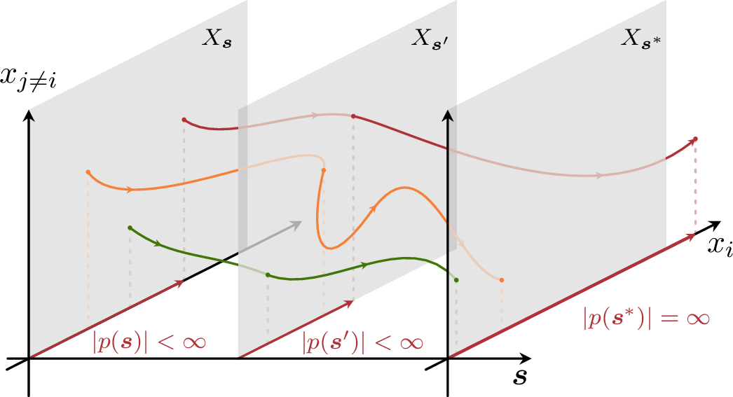
To this end, we let \(p\) be an element of the solution set to 3 , \(p \in V(\mathcal{I})\), and let \(|p(\boldsymbol{s})|\) be its distance from the origin in \(X_{\boldsymbol{s}}\). Crucially, as the number of solutions to 3 degenerates at \(\boldsymbol{s} = \boldsymbol{s}^*\), then at least one solution point must run off to infinity as \(\boldsymbol{s}\to\boldsymbol{s}^*\), \[\lim_{\boldsymbol{s} \to \boldsymbol{s}^*} |p(\boldsymbol{s})| = \infty \quad \text{for some } p \in V(\mathcal{I}) \,.\] This can be seen as follows. For generic \((\boldsymbol{\nu},d)\), \(V(\mathcal{I})\) remains a finite set of isolated points for any value of \(\boldsymbol{s}\). Its cardinality can therefore drop only when a solution reaches a boundary of \(X_{\boldsymbol{s}}\).
In the coordinates \((x_0,\ldots,x_E)\), every such escape sends some coordinate to infinity: in particular, a point reaching \(\{x_i=0\}\) or \(\{\mathcal{G}=0\}\) makes \(x_0=1/(x_1\cdots x_E\,\mathcal{G})\to\infty\), while \(\{x_{i>0}=\infty\}\) is direct. The proposed strategy is thus to track the values of \(\boldsymbol{s}\) for which this singular behaviour is observed. This is illustrated in 1.
Ideal Projections.Identifying when a solution diverges to infinity for a multivariate system of polynomial equations is at first sight a difficult problem. It is thus illustrative to look at the univariate case first, where ideals are generated by a single polynomial, \[\label{eq:ideal95univ95ex} \mathcal{I}_{\text{univ}}(\boldsymbol{a}) = \left\langle a_0 + a_1 x \cdots+a_{m-1}x^{m-1} + a_m x^m \right\rangle \,,\tag{6}\] with bounded coefficients \(a_0,\ldots,a_m\). Such a polynomial has \(m\) roots (counted with multiplicity). The only way for this number to drop is if the degree of the polynomial decreases, which can only occur if \(a_m = 0\). Indeed, in the limit \(a_m \to 0\), one root of the polynomial above escapes to infinity. In the context of Feynman integrals, \(a_m\) would thus correspond to a Landau singularity (or, more generally, a product of them).
In a multivariate setting such as 3 , there is no direct analogue of the univariate formula in 6 from which to read off the relevant coefficients. Nevertheless, one can reduce the problem to the univariate case by projecting the solution set onto one coordinate \(x_i\) at a time, before repeating the univariate analysis described above. This can be achieved by computing elimination ideals: \[\mathcal{I}_{\text{elim}}^{(i)} \equiv\mathcal{I}\cap\mathbb{Q}[x_i]\,.\] Intuitively \(\mathcal{I}_{\text{elim}}^{(i)}\) consists of all polynomial relations in \(\mathcal{I}\) involving only the variable \(x_i\). Since \(\mathcal{I}\) is zero-dimensional, \(\mathcal{I}_{\text{elim}}^{(i)}\) is generated by a single univariate polynomial whose roots are precisely the \(x_i\)-coordinates of the solution points \(p\), \[\mathcal{I}_{\text{elim}}^{(i)} = \left\langle c^{(i)}_0(\boldsymbol{s}) + \cdots + c^{(i)}_m(\boldsymbol{s}) x_i^m \right\rangle\,. \label{eq:elim}\tag{7}\] Exactly as in the univariate example, an \(x_i\)-coordinate can diverge only when the leading coefficient vanishes, so \(c^{(i)}_m(\boldsymbol{s})\) contains a subset of the Landau singularities of the Feynman integral. By iterating the procedure over all \(i \in \{0,\ldots,E\}\), then all singularities will be captured.
Computing the elimination ideal in 7 requires computing Gröbner bases and polynomial reductions modulo them, which can become prohibitively expensive. We sidestep much of this cost by working over finite fields: the
recently released linear-algebraic reduction package SP\(\mathbb{Q}\)R [28], through
FiniteFlow [30], makes such projections feasible even for the many (kinematic) scale polynomial systems generated by Feynman
integrals.
Decomposition in Sectors.In practice, the computation of \(\chi\) can be greatly simplified by stratifying the problem into sectors of the Feynman integral in 1 . Setting \(\boldsymbol{\nu}=0\) in 2 replaces \(\mathcal{I}\) by \[\label{eq:chi95ideal95unreg} \mathcal{J} \equiv \langle \partial_1 \mathcal{G},\,\ldots,\,\partial_E\mathcal{G},\,1-x_0\,\mathcal{G} \rangle \,.\tag{8}\] \(\chi_{\mathcal{S}}\equiv\deg(\mathcal{J})\) counts the master integrals of the top sector (equivalently, the maximal cut) of the diagram [24]. The same construction can be applied to every sector \(\mathcal{S}\): \[\mathcal{J_\mathcal{S}} \equiv \langle \partial_1 \mathcal{G}_\mathcal{S},\,\ldots,\,\partial_E\mathcal{G}_\mathcal{S},\,1-x_0\,\mathcal{G}_\mathcal{S} \rangle \,,\] where the sector polynomial \(\mathcal{G}_\mathcal{S}\) is obtained from \(\mathcal{G}\) by sending combinations of \(x_i \to 0\), which is graphically equivalent to contracting the corresponding internal edges to points. When the \(\boldsymbol{\nu}=0\) specialisation is well-behaved, summing the sector contributions recovers the full Euler characteristic, \[\label{eq:euler95chi95sector95sum} \chi = \sum_{\mathcal{S}\in \text{sectors}} \chi_\mathcal{S}\,.\tag{9}\] Finding singularities then reduces to checking whether any individual \(\chi_\mathcal{S}\) drops from its generic value, using the same elimination strategy applied to each \(\mathcal{J}_\mathcal{S}\).
This decomposition provides substantial computational benefit, splitting one large computation into many small ones. However, it is optional: one may always work directly with the full ideal in 3 , at the price of a higher computational cost.
Importantly, the \(\boldsymbol{\nu}=0\) specialisation may carry subtleties, which manifest themselves as 9 failing to hold. We discuss these in 6, where we also provide efficient diagnostic tests that detect such situations.
3 A Working Example↩︎
Two-Loop Equal-Mass Sunrise.To illustrate the methods discussed in 2 it is useful to work through a simple example. To this end we consider \[\begin{align} \label{eq:sunriseG} &\includegraphics[valign=c]{figures/diagram_sunset}\notag\\ \mathcal{G}&_{\text{sun}}(\boldsymbol{x},s,m) = x_1 x_2 + x_1 x_3 + x_2 x_3 + s\,x_1 x_2 x_3 \\& -m^2\, (x_1+x_2+x_3)(x_2x_3+x_1x_2+x_1x_3) \notag\,, \end{align}\tag{10}\] namely a two-loop equal-mass sunrise diagram. Using 8 we find that \(\deg(\mathcal{J}_{\text{sun}})=\chi_{\mathcal{S}}=4\), where \(\mathcal{S}=\{1,1,1\}\) is the top sector including all three propagators. This is in agreement with the well-known fact that there are four master integrals (without accounting for symmetries) in the top sector of this diagram. To find the Landau singularities one proceeds by projecting down \(\mathcal{J}_{\text{sun}}\) onto each coordinate axis. For \(x_0\) this results in a cubic polynomial: \[\mathcal{J}_{\text{sun}} \cap \mathbb{Q}[x_0] = \left\langle c_0^{(0)}+c_1^{(0)}x_0+c_2^{(0)}x_0^2+c_3^{(0)}x_0^3 \right\rangle\,.\] Thus, the Euler characteristic drops when \(c_3^{(0)}=0\). Indeed an explicit computation shows that \[c_3^{(0)}=16\,s\,,\] which produces the Landau singularity \(\{s\}\). The procedure can now be repeated for the other coordinates. For \(x_1\) the projection results in a quartic polynomial \[\label{eq:sunrise95ideal} \mathcal{J}_{\text{sun}} \cap \mathbb{Q}[x_1] = \left\langle c_0^{(1)}+\cdots+c_4^{(1)}x_1^4 \right\rangle\,,\tag{11}\] where explicitly the top coefficient is given by \[c_4^{(1)}=9\, m^2 \left(m^2-s\right)^2 \left(9 m^2-s\right)\,.\] Thus, \(\{m,s-m^2,s-9m^2\}\) are identified as further Landau singularities. Repeating this procedure for the remaining two coordinates results in no new factors. By combining the singularities from all projections the full set is thus given by \(\boldsymbol{l}(s,m)=\{s,m,s-m^2,s-9m^2\}\), reproducing the well-known standard result [17], [38].
This result, and many others, can automatically be produced with the proof-of-concept Mathematica routine SPQRLandau available from the repository :
G = x1 x2 + x1 x3 + x2 x3 + s x1 x2 x3
    - m^2 (x1 + x2 + x3)(x2 x3 + x1 x2 + x1 x3);
vars = {x1, x2, x3};
SPQRLandau[G, vars] (* Out: {m^2,s,s-9m^2,s-m^2} *)
4 New Results↩︎
The new method of 2 is especially suited to the cutting-edge bottleneck diagrams, namely (near) maximally connected graphs. [fig:new95applications] shows three such examples. Their Landau singularities have been studied in the past, but the full set had remained beyond the reach of all currently available tools. In fact, every method we are aware of (e.g., [9], [20], [21], [27]) either stalls or produces incomplete lists of singularities for these examples.
Using the method introduced above, all known singularities of [39] were reproduced and a new set of singularities was resolved for all three families.
Figure 2: 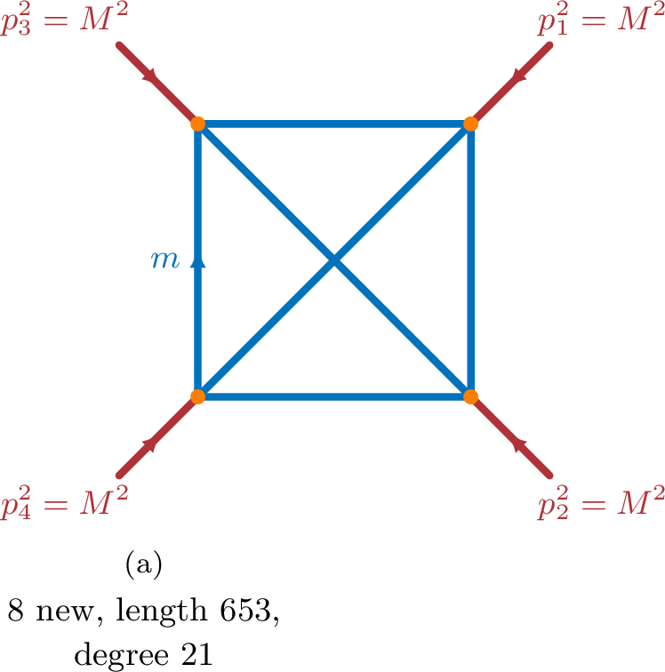 .
.
Figure 3: 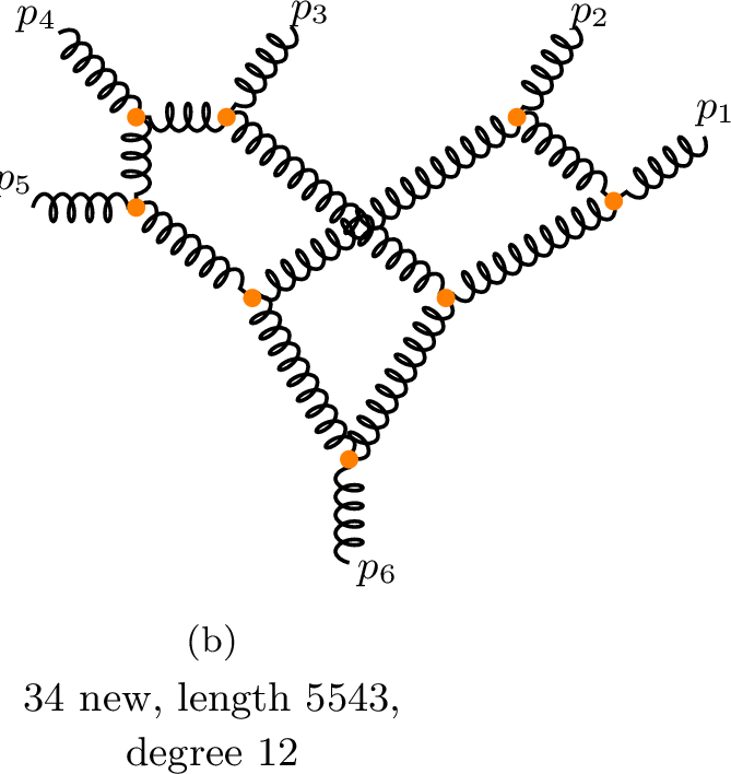 .
.
Figure 4: 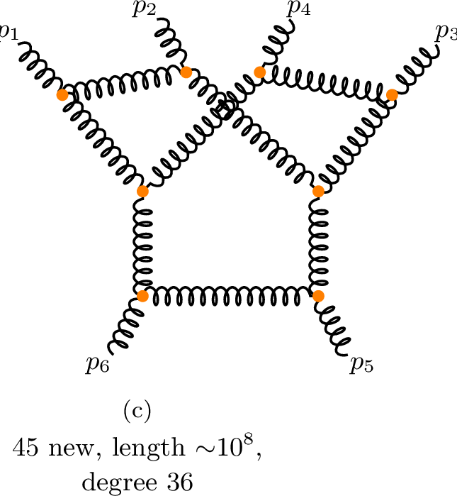 .
.
For each of the three families the diagnostic tests of 6 were run. A small fraction of sectors (for example, 8% for diagram (b)) triggered the specialised degeneracy of 12 . These sectors are simple and their singularities could be computed directly by [9], while the sectors accessible only through the projection pass all diagnostic checks. To the best of our understanding, therefore, no genuine singularity has been missed by our analysis, and we regard these lists as complete. The full set of singularities can be found in the repository .
Perhaps one of the most surprising things about the additional sets of singularities obtained for these diagrams is the remarkable size and high polynomial degree of some of them, as documented in [fig:new95applications] 1.
We note that SPQRLandau is intended as a proof-of-concept function and is not optimised sufficiently to tackle the diagrams of [fig:new95applications]. These integrals required a manual optimisation of the finite-field sampling pipeline. A full automation of this procedure is left to future work.
\(\boldsymbol{d=4}\) Kinematics.The above results are computed assuming \(d\)-dimensional external kinematics, both to stress-test the method and to benchmark against PLD [19], [20] and [9], which operate by default under this assumption. The singularity lists can be restricted to four-dimensional external kinematics [43], using the parametrisation of 7. We find that all restricted singularities are genuine (see the discussion around 15 for details). Both \(d\)- and four-dimensional lists are provided in the repository 2.
5 Discussion↩︎
In this Letter we have introduced a new method for determining the Landau singularities of a Feynman integral. The method extracts the entire Landau locus directly by tracking the kinematic configurations at which the Euler characteristic drops, that is, where critical points escape to infinity. Working over finite fields renders the underlying elimination tractable even for many-scale, multi-loop integrals. The output, subject to verified diagnostic checks, is the strict set of singularities rather than a superset. For complicated polylogarithmic Feynman integrals at the precision frontier, working with the exact set could dramatically reduce the effort needed to construct symbol letters from candidate singularities [45].
We have illustrated the method on bottleneck diagrams beyond the reach of existing tools, namely the two hardest non-planar six-point two-loop graphs and the non-planar massive envelope in [fig:new95applications]. We provide a proof-of-concept implementation together with an extensive cross-check against [9]. Although suppressed in colour relative to their recently computed planar counterparts [46]–[48], the non-planar contributions to the six-gluon amplitude in [fig:new95applications] (b,c) should soon be tackled by the community. The singularities found in this work, together with their four-dimensional restriction discussed in 4, should be essential to that effort.
Several directions invite further work. On the algorithmic side, interfacing the elimination step with dedicated solvers such as msolve [49]
should extend the reach to still more complex topologies. A finer understanding of the factored structure of the projected polynomials, including the multiplicities with which individual singularities appear, would further improve performance. It would
also be worthwhile to evaluate the Euler characteristic in alternative representations, such as the loop-by-loop Baikov representation [33], [50], where, leaving subtleties aside, the relevant ideals can be considerably smaller and their generators far more decoupled.
While not the focus of this Letter, the method also applies to integrals with non-trivial numerators and non-standard (e.g., linearised or eikonal) propagator structures. Indeed, such integrals also admit a Lee-Pomeransky representation. It would be interesting to study on a large set of examples cases in which singularities cancel in the presence of numerators. A systematic understanding of such cancellations could have important applications in amplitude bootstrap methods of, e.g., the Standard Model.
Finally, we expect the tools introduced in this Letter to converge into an automated Mathematica package.
Acknowledgments.
We would like to thank Miguel Correia, Sebastian Mizera, Erik Panzer, and Tiziano Peraro for stimulating discussions. We thank Luke Lippstreu, Andrew J. McLeod, and Maria Polackova for allowing us to share functions from the DiscKosky
package before release, as well as many interesting and fruitful discussions. We furthermore thank Franz Herzog and the Institute for Advanced Study for generously lending significant computational resources throughout the duration of this project. The
research of V.C. is funded by the European Research Council (ERC) Synergy Grant MaScAmp 101167287. The research of G.C. is supported by the United Kingdom Research and Innovation grant UKRI FLF MR/Y003829/1. M.G. is supported by the U.S. Department of
Energy (DOE) grant No. DE-SC0011941.
6 Subtleties with the Sectors Approach↩︎
The sector decomposition 9 rests on the specialisation \(\boldsymbol{\nu}=0\), which can fail in four known ways. These fall into two families. In the first, a solution set of
\(\mathcal{J}_\mathcal{S}\) becomes positive-dimensional and, in the second, a critical point escapes to infinity as \(\boldsymbol{\nu}\to 0\). Within each family the failure is either
generic or confined to a special kinematic slice \(\boldsymbol{s}^*\). We label the cases accordingly, as Type 1.1 and Type 1.2 for positive-dimensional solutions
and Type 2.1 and Type 2.2 for the case of points at infinity. The first three can result in missing genuine singularities, whereas Type 2.2 can instead generate
fictitious ones. All are rare and inexpensive to detect, as explained below. These routines are implemented with the upcoming Mathematica package DiscKosky [51], a beta for which can be downloaded at [52]. All data from this appendix is
reproduced in the repository .
As noted in the main text, the examples of 4 are free of these caveats, the sole exception being a few simple sectors manifesting Type 1.2, whose problematic singularities can resolve directly with ease.
Type 1.1: General Higher-Dimensional Solutions.For generic \(\boldsymbol{\nu}\), as in 3 , the solution set is always zero-dimensional. At \(\boldsymbol{\nu}=0\) this can break: for certain degenerate sector polynomials \(\mathcal{G}_\mathcal{S}\), the solutions of \(\mathcal{J}_\mathcal{S}\) form positive-dimensional families rather than isolated points. In ideal language, this corresponds to the condition \(\dim(\mathcal{J}_\mathcal{S})\neq 0\). This behaviour has also been tied to the “magic relations” that break the notion of sectors and cuts [53].
Figure 5: 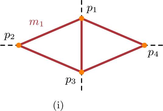 .
.
Figure 6: 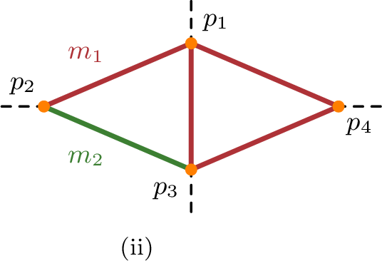 .
.
Figure 7: 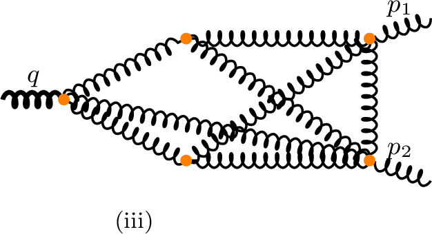 .
.
The diagnostic is therefore to check whether \(\dim(\mathcal{J}_\mathcal{S})=0\) on a generic kinematic slice for each sector. A sector with \(\dim(\mathcal{J}_\mathcal{S})\neq 0\)
signals a failure of 9 . In practice the computation of \(\dim(\mathcal{J}_\mathcal{S})\) is computationally inexpensive, and DiscKosky [51] evaluates it directly through the function CountSectorsUnregulated, returning Indeterminate if \(\dim(\mathcal{J}_\mathcal{S})\neq 0\). An example is the equal-mass “acnode” in [fig:app95diags] (i), where the top sector manifests a
higher-dimensional solution:
vars = {x1, x2, x3, x4, x5};
CountSectorsUnregulated[Gi, vars, vars]
(* Out: Indeterminate *)
Type 1.2: Specialised Higher-Dimensional Solutions.Even when \(\dim(\mathcal{J}_\mathcal{S}(\boldsymbol{s}))=0\) generically, the ideal dimension can jump at a special location: \(\dim(\mathcal{J}_\mathcal{S}(\boldsymbol{s}^*))\neq 0\). The singularities causing this behaviour must manifest in a very specific (and problematic) form. To see this, let \[\mathcal{J}^{(i)}_{\mathcal{S},\text{elim}}\equiv \mathcal{J}_{\mathcal{S}} \cap \mathbb{Q}[x_i]\,.\] If \(\dim(\mathcal{J}_\mathcal{S}(\boldsymbol{s}^*))\neq 0\), then necessarily for at least one \(x_i\) \[\dim(\mathcal{J}^{(i)}_{\mathcal{S},\text{elim}}(\boldsymbol{s}^*))\neq 0\,.\] Since \(\mathcal{J}^{(i)}_{\mathcal{S},\text{elim}}\) is generated by a univariate polynomial, it can only be non-zero-dimensional if all coefficients vanish on \(\boldsymbol{s}^*\). It follows that \[\label{eq:degenerate95factoring} \mathcal{J}^{(i)}_{\mathcal{S},\text{elim}} = \left\langle\, l_\text{degen}(\boldsymbol{s})\left (\tilde{c}_0^{(i)} + \cdots + \tilde{c}_n^{(i)} x_i^n \right) \right\rangle\,,\tag{12}\] where \(l_\text{degen}(\boldsymbol{s}^*)=0\). Conservatively, it should be assumed that \(l_\text{degen}\) could be a genuine Landau singularity where \(\dim(\mathcal{I})\) drops in value. The difficulty is that SP\(\mathbb{Q}\)R reconstructs Gröbner bases over the ring \(R = \mathbb{Q}(\boldsymbol{s})[\boldsymbol{x}]\), that is, polynomials in the integration variables \(\boldsymbol{x}\) whose coefficients are rational functions of the kinematics \(\boldsymbol{s}\). Over this ring, every ideal element is defined only up to a kinematic prefactor (fixed by normalising the coefficient of one monomial to \(1\) in each generator). The factor \(l_\text{degen}\) is therefore absorbed in this arbitrary prefactor, rendering it invisible.
It is thus important to test whether such a singularity can occur. The diagnostic is to recompute the same ideal \(\mathcal{J}_\mathcal{S}\) over the ring \(\mathbb{Q}(s_2,\ldots)[s_1,\boldsymbol{x}]\), promoting one kinematic variable \(s_1\) to a polynomial variable. Elimination over this ring cannot divide out a degenerate singularity that depends on \(s_1\), so its presence becomes visible.
In practice, several numerical evaluations on this ring suffice, making this test inexpensive. The algorithm is included in the repository as noDegeneracyQ. If this
function returns True, no singularity of the form 12 can occur. We find that Feynman diagrams violating this condition are rare.
The “deformed acnode” in [fig:app95diags] (ii) illustrates this behaviour. One can explicitly verify that
noDegeneracyQ[Gii, vars][[1]] (* Out: False *)flagging that the sector-by-sector elimination is not guaranteed to capture every singularity here. The missed component is \(l_\text{degen}=m_1^2-m_2^2\). Indeed, specialising to this kinematic locus results in the example previously considered in [fig:app95diags] (i). Note that singularities manifesting this behaviour seem to be extremely simple, and are captured with ease by . This example is provided in more detail in the repository .
Type 2.1: Bulk Solutions at Infinity.The two modes above concern solutions becoming positive-dimensional. A different effect can arise even when \(\dim(\mathcal{J}_{\mathcal{S}})=0\): a critical point lying at a finite (bulk) point of \(X_{\boldsymbol{s}}\) for generic \(\boldsymbol{\nu}\) can be pushed to infinity in the limit \(\boldsymbol{\nu}\to0\). Such a point is then absent from \(\mathcal{J}_{\mathcal{S}}\), so \(\chi_{\mathcal{S}}\) undercounts the true number of critical points [54].
The method of checking whether this may occur is very simple. One verifies that 9 holds before proceeding to the elimination step. Since each \(\chi_\mathcal{S}\) is only
known to undercount, this equality is sufficient to rule out the issue for all sectors of the diagram. The four-loop form factor given in [fig:app95diags] (iii)
realises this phenomenon [55]. An explicit computation reveals that \[\chi = 13\,,\qquad \sum_{\mathcal{S}\in
\text{sectors}}\chi_\mathcal{S} = 12\,,\] where a critical point attributable to the top sector is manifestly missing in the sector-by-sector approach. Once again, using the package DiscKosky this can be explicitly verified by comparing
the outputs of the functions CountSectorsUnregulated and CountSectorsRegulated. Explicitly we have
chiReg = CountSectorsRegulated[Giii,vars,{}];
chiSbS = CountSectorsUnregulated[Giii,vars,{}][[1]];
chiReg == chiSbS (* Out: False *)
Type 2.2: Fictitious Singularities at Infinity.The sector-by-sector computation can in rare cases over-count. In the elimination step, a locus \(\boldsymbol{s}^*\) is flagged whenever a solution of the specialised ideal \(\mathcal{J}_\mathcal{S}\) runs to infinity as \(\boldsymbol{s}\to\boldsymbol{s}^*\). While this produces genuine singularities in almost all cases, it can happen instead that this behaviour is an artefact of the \(\boldsymbol{\nu}=0\) sector specialisation. In this case no regulated critical point is lost, as \(\chi\) does not drop at \(\boldsymbol{s}^*\): \[\chi(\boldsymbol{s}) = \chi(\boldsymbol{s}^*) > \sum_\mathcal{S}\chi_\mathcal{S}(\boldsymbol{s}^*)\,.\] The corresponding factor is thus fictitious. Such examples are not ruled out by the Type 2.1 diagnostic, which checks the generic count \(\chi=\sum_\mathcal{S}\chi_\mathcal{S}\) for generic \(\boldsymbol{s}\), away from \(\boldsymbol{s}^*\).
The diagnostic is again inexpensive. Once the candidate singularities are obtained, each is verified against 5 at generic \(\boldsymbol{\nu}\), and any that does not correspond to a genuine drop is discarded.
An example of this occurring can be found again in the “deformed acnode” graph discussed already in the context of Type 1.2. For this diagram, the top sector Euler characteristic drops from \(4\) to \(3\) on the “singularity” given by \(l_{\text{spur}}=m_1^2\,s_{12}+m_2^2\,s_{23}+s_{12}\,s_{23}\) . Nevertheless, a computation with the fully regulated
Euler characteristic returns no drop. Using DiscKosky,
lspur = mm1 s12 + mm2 s23 + s12 s23;
CountSectorsUnregulated[Gii,vars,{}][[1]](* Out:4 *)
CountSectorsUnregulated[Gii,vars,{},
                "Constraint"->lspur][[1]](* Out:3 *)
CountSectorsRegulated[Gii,vars,{}]      (* Out:30 *)
CountSectorsRegulated[Gii,vars,{},
                  "Constraint"->lspur]  (* Out:30 *)
Diagnostic Pipeline.Collecting the above checks:
Type 1.1] \(\dim(\mathcal{J}_{\mathcal{S}})=0\) for every sector \(\mathcal{S}\), ruling out general higher-dimensional solutions.
Type 1.2] noDegeneracyQ returns True for every sector \(\mathcal{S}\), ruling out specialised higher-dimensional solutions.
Type 2.1] \(\chi=\sum_\mathcal{S}\chi_\mathcal{S}\) holds explicitly, ruling out bulk solutions at infinity.
Type 2.2] each candidate singularity is verified against 5 at generic \(\boldsymbol{\nu}\), discarding any fictitious ones.
With all four tests passed, the method of 2 returns all Landau singularities, barring any as-yet-undiscovered failure mode. For the vast majority of Feynman diagrams the four conditions hold, so the scope of the method
remains broad. This full diagnostic pipeline is automatically implemented in the demo function SPQRLandau.
Finally, it should be noted that if any of the above criteria are not satisfied, it is still possible to compute \(\chi\) directly from the regularised ideal in 3 . As argued in the main text, this strategy will in principle work for all Feynman integrals. Nevertheless, this will come at some computational cost due to the increased complexity of \(\mathcal{I}\) compared to the much simpler set \(\mathcal{J}_{\mathcal{S}}\).
7 Restriction to 4d Kinematics↩︎
In the main text, the six-point singularities are computed with \(d\)-dimensional external kinematics, imposing no constraints among the Mandelstam invariants besides total momentum conservation. For phenomenological applications one often restricts the external momenta to span at most a four-dimensional subspace (the ’t Hooft–Veltman scheme [43]). This appendix provides an explicit parametrisation.
We consider six massless momenta \(p_1,\ldots,p_6\) with \(p_i^2=0\) and \(\sum_{i=1}^6 p_i=0\). In generic dimension there are nine independent Mandelstam invariants. In four dimensions the Gram matrix \(G_{ij}=2\,p_i\cdot p_j\) of \(p_1,\ldots,p_5\) must have vanishing determinant, removing one degree of freedom.
We realise this constraint by writing \(p_5 = \sum_{i=1}^4 a_i\, p_i\), which forces \(\det G = 0\) identically. The sub-kinematics of \(p_1,\ldots,p_4\) is parametrised by six invariants \(\{s_{12},s_{23},s_{34},s_{123},s_{234},s_{1234}\}\) with \(s_{1234}\equiv s_{56}\), giving \[\begin{align} \label{eq:4d95dotproducts} & p_i{\cdot}p_{i+1} = \tfrac{s_{i\, i+1}}{2}\,, \, p_i{\cdot}p_{i+2} = \tfrac{1}{2}(s_{i\,i+1\,i+2}{-}s_{i\,i+1}{-}s_{i+1\,i+2})\,,\notag \\& p_1{\cdot}p_4 = \tfrac{1}{2}(s_{1234}{-}s_{123}{-}s_{234}{+}s_{23})\, \quad (1\leqslant i\leqslant 3)\,. \end{align}\tag{13}\] Imposing \(p_5^2=0\) and \(p_6^2=0\) (with \(p_6=-\sum_{i=1}^5 p_i\)) and solving for, e.g., \(s_{12}\) and \(s_{23}\) yields \[\begin{align} \label{eq:4d95gauge} s_{12} &= \frac{N_{12}}{a_2-a_3}\,,\qquad s_{23} = \frac{N_{23}}{(a_1{-}a_2)(a_3{-}a_4)}\,, \end{align}\tag{14}\] with the numerators given in the repository . In this case, the eight free variables are thus \(\{s_{34},\, s_{123},\, s_{234},\, s_{1234},\, a_1,\, a_2,\, a_3,\, a_4\}\). Explicit substitution rules are also provided there.
The substitution is rational in the external invariants, so specialising the Lee–Pomeransky polynomial \(\mathcal{G}\) gives the ratio \(\mathcal{G}\big|_{\rm 4d}=\mathcal{G}_{\rm HV}/f(a)\), with \(\mathcal{G}_{\rm HV}\) the polynomial numerator and \(f(a)\) a purely kinematic denominator. The polynomial \(\mathcal{G}_{\rm HV}\) is the ’t Hooft–Veltman polynomial, on which the singularity analysis of 2 can be re-run. The restricted integral therefore reads \[\label{eq:4d95prefactor} I_{\boldsymbol{\nu}}\big|_{\rm 4d} \propto f(a)^{d/2} \int_0^\infty \boldsymbol{x}^{\boldsymbol{\nu}}\,\mathcal{G}_{\rm HV}(\boldsymbol{x},\boldsymbol{s})^{-d/2}\,\frac{\mathrm{d}\boldsymbol{x}}{\boldsymbol{x}}\,.\tag{15}\] Because \(f(a)\) carries no \(\boldsymbol{x}\)-dependence, it drops out of the critical-point ideal , and its zeros therefore need not lower \(\chi\). Nonetheless, \(f(a)^{d/2}\) generates a genuine branch point of \(I_{\boldsymbol{\nu}}\) at \(f(a)=0\), so these loci are genuine Landau singularities.
Although specialising kinematic parameters and computing singularities do not commute in general [19], for diagrams (b, c) of [fig:new95applications] the two procedures agree upon direct computation: (i) restricting the \(d\)-dimensional singularity list to four-dimensional kinematics, and (ii) re-running the singularity analysis directly on \(\mathcal{G}_{\rm HV}\) and adjoining the prefactor singularities \(f(a)=0\), produce the same set of singularities. Apart from these prefactor singularities, every factor arising upon restriction remains genuine in the sense of a \(\chi\)-drop of 5 .
References↩︎
SubTropica, arXiv preprint (2026), https://arxiv.org/abs/2604.20954.msolve: A Library for Solving Polynomial Systems, in https://doi.org/10.1145/3452143.3465545, 46th
International Symposium on Symbolic and Algebraic Computation(ACM, Saint Petersburg, Russia, 2021) pp. 51–58.We furthermore independently verified the drop in the number of master integrals near these singularities using IBP identities [40], [41] on fully numerical slices, generated with the private Mathematica package FFIntRed by Tiziano Peraro and solved by a variant of the Laporta algorithm [42] based on the finite-field arithmetic and functional reconstruction framework of FiniteFlow [30].↩︎
We also cross-checked the corresponding Euler characteristics for each sector using IBP identities, following the strategy of [44].↩︎