¹

²

1 Introduction↩︎

Coherent links between separated quantum systems are a basic ingredient of modular quantum processors and quantum networks [1], [2]. In such an architecture, small processors can be fabricated, controlled and diagnosed as separate units, while itinerant carriers distribute quantum states and entanglement between them. Most experimental links encode one qubit per carrier or per node, but a larger local Hilbert space can change what a network link can transmit. A qutrit carries a three-dimensional quantum state, and two qutrits can host entanglement with Schmidt rank three, which cannot be embedded in any two-qubit state. Such high-dimensional resources can increase dense-coding capacity, support qudit Bell inequalities and provide a larger alphabet for quantum communication, quantum computation and quantum metrology [3]–[7]. In optics, high-dimensional photonic states have become a central resource for quantum communication protocols [8]–[11]. High-dimensional qudits have also been controlled and entangled in local trapped-ion processors and solid-state spin registers [12]–[14], demonstrating the hardware potential of qutrit and qudit encoding. Extending this capability from local processors to remote nodes, however, requires a link that can transfer and entangle full three-level quantum states rather than a single two-level subspace. At the network level, such resources could also enable high-dimensional Bell-type protocols with ternary outcomes, extending recent superconducting-circuit demonstrations of loophole-free Bell tests and device-independent randomness amplification from binary qubit correlations toward qutrit correlations [15], [16].

Superconducting circuits provide a natural platform for testing whether this high-dimensional network picture can be made deterministic in the microwave domain. Circuit QED combines strong artificial atom-resonator coupling with shaped microwave emission and time-reversed capture [17], enabling deterministic state transfer and remote entanglement between superconducting qubits and microwave cavity memories [18]–[24]. At the same time, the higher transmon levels are native degrees of freedom rather than added hardware, and local qutrit control, benchmarking and multi-qutrit gates have developed rapidly [25]–[30]. A remote qutrit link, however, requires more than reusing a qubit link with a larger local basis. It must map the two non-ground amplitudes onto two temporal modes of the same waveguide, preserve their calibrated relative phase, and avoid opening all qutrit transitions to the continuum at once. Here we demonstrate qutrit-level quantum communication between two independently packaged superconducting nodes connected by a one-metre microwave link. Each node contains a transmon qutrit, an auxiliary resonator and a tunable Purcell-filter interface. The auxiliary resonator provides a transition-selective interface between the stored qutrit and the travelling microwave field: only the addressed qutrit–resonator sideband is opened, while the other qutrit amplitude remains stored in the transmon. This is the key difference from a direct qubit–waveguide interface, where opening the radiative channel generally exposes all allowed transmon transitions to the same continuum. The Purcell filter controls the coupling decay rate \(\kappa_c\) from the auxiliary resonator into the waveguide, while the transmon flux bias controls the dressed auxiliary-resonator frequency through the dispersive Lamb shift. With these two knobs we match both the resonant frequency and the photon bandwidth of the two remote interfaces in situ [31]. We then send the qutrit amplitude in two time bins through the same cascaded channel, using an \(e0g1\) flux-parametric sideband [32] for the \(\ket{e}\) component and an \(f0g1\) cavity-assisted Raman process [20], [22], [33] for the \(\ket{f}\) component.

The results cross the qubit boundary in three experimentally reconstructed ways. First, qutrit state transfer gives a mean transferred-state fidelity of \(83.68\%\), above the classical qutrit measure-and-prepare limit \(1/2\) and the maximum average fidelity \(3/4\) for transmitting an arbitrary qutrit through an effective two-dimensional channel. Quantum process tomography of the same transfer protocol gives \(F_{\chi}=77.12\%\), above the corresponding process-fidelity bounds \(1/3\) and \(2/3\) [34], [35]. Second, by reducing the primitive pulse areas, the same hardware generates a remote two-qutrit maximally entangled state \((\ket{gf}+\ket{ee}+\ket{fg})/\sqrt{3}\): its fidelity exceeds the Schmidt-rank-two bound \(2/3\), and its negativity is \(0.730\), above the maximum \(0.5\) for any two-qubit state [36]–[39]. Third, the reconstructed ensemble-averaged density matrix gives a tomography-inferred dense-coding capacity of \(2.273\) bits, above the classical qutrit value \(\log_2 3\) and the ideal qubit dense-coding limit of 2 bits [3]–[5], together with a tomography-inferred Collins–Gisin–Linden–Massar–Popescu (CGLMP) Bell parameter \(I_3=2.332\), above the local bound of 2 [6]. These measurements show that the same microwave link can act as a coherent three-level channel and as a source of high-dimensional entanglement.

2 Tunable-interface architecture and qutrit protocol↩︎

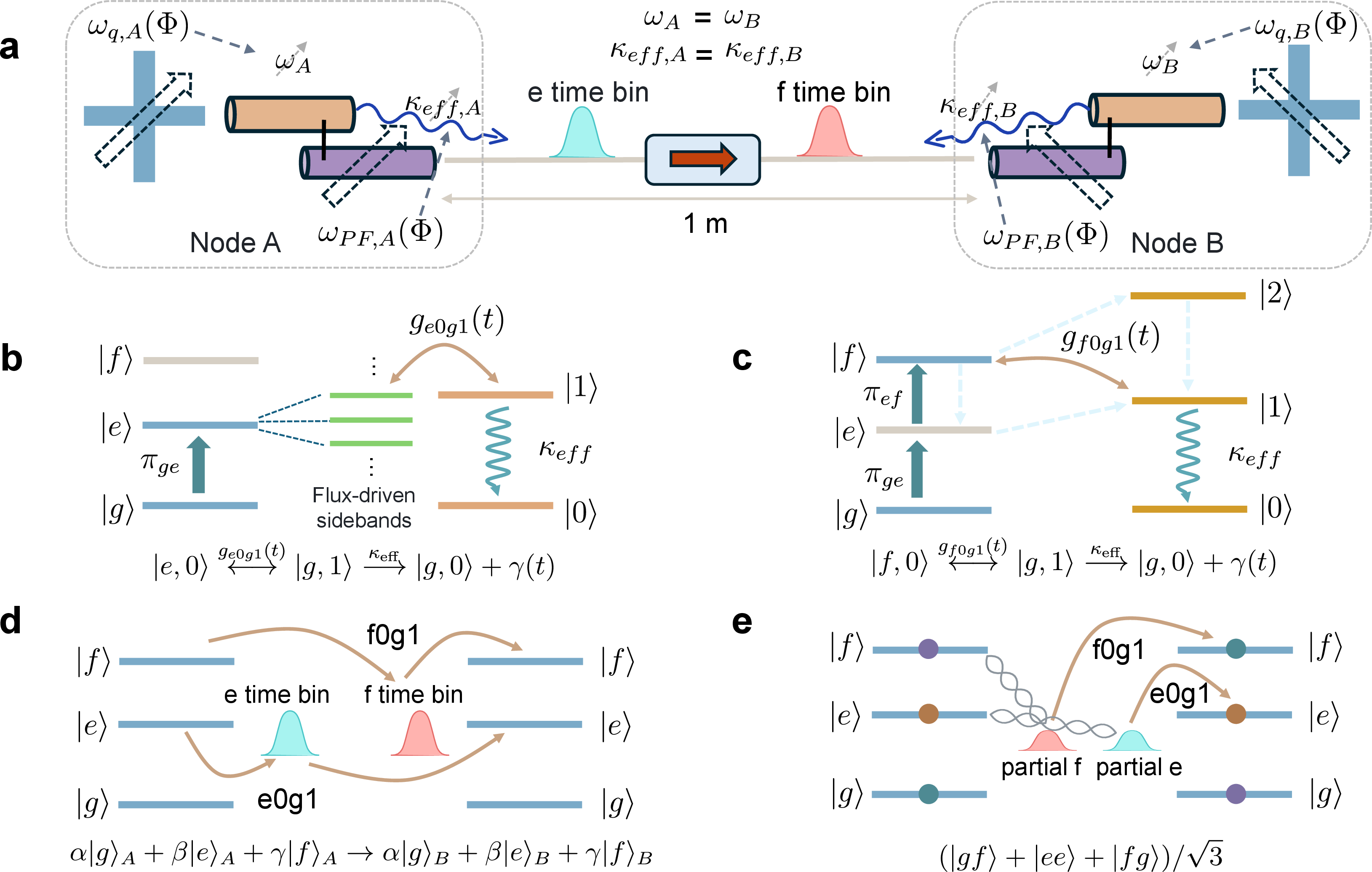
The device architecture is shown schematically in Fig. 1a. The two superconducting nodes are mounted in separate sample boxes and connected by a one-metre microwave cable. Each node contains a transmon qutrit [40], with logical states \(\{\ket{g},\ket{e},\ket{f}\}\), and a transmission resonator that emits and captures itinerant photons. A tunable Purcell filter couples the transmission resonator to the cascaded waveguide [41]–[43]. The resulting interface has two independent matching knobs. The transmon flux bias shifts the dressed transmission-resonator frequency through the dispersive Lamb shift, while the Purcell-filter bias changes the loaded linewidth and hence the photon bandwidth. We use these knobs to bring the two remote interfaces to a common operating frequency near \(7.4347~{\rm GHz}\) and to choose comparable radiative linewidths; the corresponding spectroscopy and linewidth data are given in Supplementary Figs. S4 and S5.

The qutrit channel is built from two transition-selective photon-mediated primitives, labelled \(e0g1\) and \(f0g1\), as illustrated in Fig. 1b,c. The \(e0g1\) primitive couples \(\ket{e,0}\) and \(\ket{g,1}\) of a single node, where the second label denotes the photon number in the transmission resonator. We implement this coupling by applying a flux-parametric modulation to the transmon at the qubit–transmission-resonator detuning frequency [32], [44]. In the rotating frame, this modulation activates an effective sideband interaction that converts a transmon \(\ket{e}\) excitation into one transmission-resonator photon, or the reverse process. In the link experiment, this sideband turns the transmission resonator into a temporary output interface for the \(\ket{e}\) amplitude: node A emits the photon, and a time-delayed partner pulse at node B absorbs the same temporal mode into the remote transmon.

The \(f0g1\) primitive addresses the \(\ket{f}\) component through a cavity-assisted Raman process, like the Raman-type microwave reset and photon-mediated transfer protocols in circuit QED [20], [22], [33]. The Raman control couples \(\ket{f,0}\) to \(\ket{g,1}\) through the transmission-resonator mode while the \(\ket{e}\) amplitude is left largely stored. The transmission resonator therefore plays a dual role: it is the impedance-matched port to the waveguide, and it is the intermediate mode that makes the port transition selective. This allows the \(\ket{e}\) and \(\ket{f}\) amplitudes to be emitted and captured in different time windows without adding a second physical channel.

Both primitives are implemented with chirped \(200~{\rm ns}\) sine pulses. The sine envelope shapes the emitted microwave field into a near time-symmetric temporal mode, so that a delayed partner pulse with the same envelope approximates time-reversed capture at the receiver. The chirp compensates the amplitude-dependent transition-frequency shift during the pulse: for \(e0g1\), this shift comes mainly from the flux-modulation-induced time-averaged transmon-frequency shift, while for \(f0g1\) it comes mainly from the Raman-drive-induced ac Stark shift. The chirp profiles are independently calibrated from amplitude-to-frequency measurements for the two primitives, as shown in Supplementary Fig. S6. Full-transfer \(e0g1\) and \(f0g1\) operations implement the qutrit state-transfer map in Fig. 1d, while partial-transfer operations generate the time-bin-mediated entanglement resource shown in Fig. 1e. The calibrated receiver-pulse delays are \(8~{\rm ns}\) for \(e0g1\) and \(13~{\rm ns}\) for \(f0g1\).

3 Primitives of microwave qutrit transfer↩︎

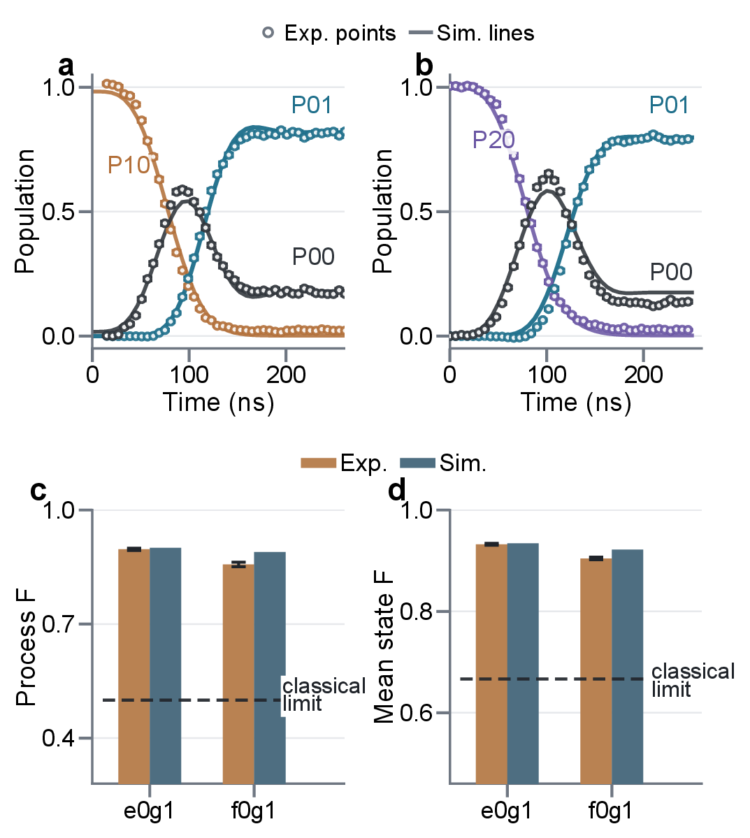
We first calibrate the elementary remote links by measuring their population dynamics. In Fig. 2, the \(\ket{e0}\leftrightarrow\ket{g1}\) and \(\ket{f0}\leftrightarrow\ket{g1}\) transfers are plotted as a function of pulse time. Node A emits the excitation with a chirped \(200~{\rm ns}\) sine pulse; node B applies the time-delayed partner pulse to absorb the same temporal mode. The sine envelope smooths the turn-on and turn-off of the effective coupling and produces a near-symmetric photon wavepacket for the calibrated bandwidth. The receiver pulse starts \(8~{\rm ns}\) after the sender pulse for \(e0g1\) and \(13~{\rm ns}\) after the sender pulse for \(f0g1\); the population traces are shown on the same measured cutoff-time axis. This is the microwave analogue of shaped-photon emission and time-reversed capture [45]–[47]. The solid curves come from a pulse-level cascaded master-equation simulation implemented with QuTiP [48]–[51]. The model uses the measured energy-relaxation rates, \(\eta_c=0.92\), \(\kappa_{{\rm int},A}/2\pi=0.0208~{\rm MHz}\), \(\kappa_{{\rm int},B}/2\pi=0.0176~{\rm MHz}\), and a \(T_1\)-corrected quasi-static \(1/f\)-like dephasing ensemble extracted from Ramsey data. The effective peak couplings used for the simulations in Figs. 2–4 are listed in the Supplementary Information; within each QPT or QST simulation these calibrated pulse parameters are held fixed across all prepared and measured states.

We characterize the two primitives as separate effective two-level transfer channels. The \(e0g1\) primitive transfers the \(\{\ket{g},\ket{e}\}\) component through the \(\ket{e,0}\leftrightarrow\ket{g,1}\) sideband, whereas the \(f0g1\) primitive transfers the \(\{\ket{g},\ket{f}\}\) component through the Raman-assisted \(\ket{f,0}\leftrightarrow\ket{g,1}\) channel. Two-level process tomography gives \(F_{\chi}=89.66 \pm 0.29\%\) for \(e0g1\) and \(85.68 \pm 0.60\%\) for \(f0g1\). The corresponding mean output-state fidelities, in the same order, are \(93.23 \pm 0.19\%\) and \(90.45 \pm 0.27\%\). These independently calibrated operations are the two building blocks combined below for full qutrit transfer.

4 Arbitrary qutrit-state transfer↩︎

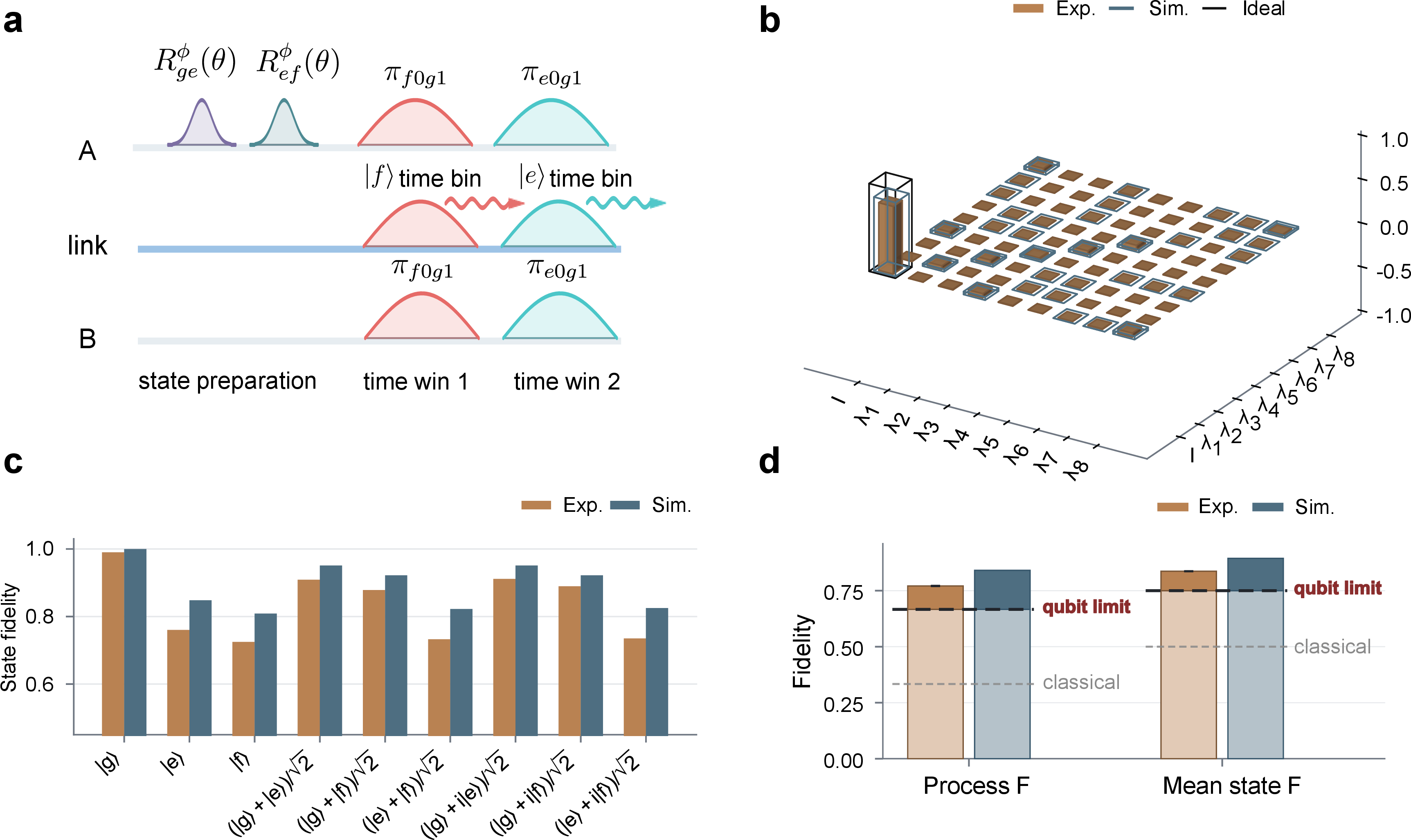
The full qutrit-transfer sequence applies the two primitives in separate temporal windows. Node A is prepared in the qutrit state to be sent and node B starts in \(\ket{g}\). The \(f0g1\) sender pulse first maps the \(\ket{f}_A\) amplitude onto a single photon in the first temporal mode; the \(e0g1\) sender pulse then maps the \(\ket{e}_A\) amplitude onto a single photon in the second temporal mode. The \(\ket{g}_A\) component is dark to both primitives and is represented by the joint vacuum of the two time bins. The flying field therefore carries a hybrid number–time-bin qutrit, \[\alpha\ket{0_1 0_2}+\gamma e^{i\varphi_f}\ket{1_1 0_2} +\beta e^{i\varphi_e}\ket{0_1 1_2},\] where \(1\) and \(2\) label the \(f0g1\) and \(e0g1\) time windows, respectively. Node B applies the time-reversed capture pulses to convert the first-bin photon to \(\ket{f}_B\) and the second-bin photon to \(\ket{e}_B\). In the ideal limit, \[\ket{e}_A\ket{g}_B \rightarrow \ket{g}_A\ket{e}_B,\qquad \ket{f}_A\ket{g}_B \rightarrow \ket{g}_A\ket{f}_B,\] while \(\ket{g}_A\ket{g}_B\) remains dark to both transfer pulses. After the two windows, \(\alpha\ket{g}_A+\beta\ket{e}_A+\gamma\ket{f}_A\) is mapped to node B, up to deterministic phases removed with calibrated drive phases and virtual-\(Z\) gates. The pulse ordering, delay scans and phase calibrations are provided in Supplementary Fig. S7.

Qutrit state tomography uses nine analysis rotations before three-state readout, and qutrit process tomography combines nine independently prepared input states with the corresponding readout-corrected output density matrices. The channel is reconstructed in the Gell-Mann basis [52]–[54]. Figure 3 compares the experimental process matrix with the pulse-level simulation and the ideal identity process in a compact overlaid representation; the complementary imaginary components and matrix-distance diagnostics are given in the Supplementary Information. The dominant identity component shows that the two time-bin primitives preserve a common qutrit phase frame, rather than acting as two independent population transfers. The residual off-diagonal terms give the remaining phase errors, leakage and dephasing accumulated during emission, propagation and capture.

Across the tested input states, the mean transferred-state fidelity is \(83.68 \pm 0.04\%\), above the classical qutrit measure-and-prepare limit of \(50\%\) and above the maximum average fidelity \(75\%\) achievable by transmitting an arbitrary qutrit through an effective qubit channel [34], [35]. The measured qutrit process fidelity is \(77.12 \pm 0.10\%\). The same pulse-level cascaded simulation gives a process fidelity of \(84.10\%\) and a mean state fidelity of \(89.45\%\), higher than the experimental values. As a separate process-matrix comparison, the matrix-distance measure \(D(\chi,\chi_{\rm sim})=\sqrt{{\rm Tr}[(\chi-\chi_{\rm sim})^2]}\), used in microwave-link process comparisons [20], gives \(D=0.141\) between the measured and simulated qutrit process matrices. The remaining experiment–simulation differences are consistent with residual calibration errors and slow parameter drifts during the long qutrit QPT acquisition that are not included in the fixed-parameter model.

5 Remote qutrit entanglement beyond the qubit limit↩︎

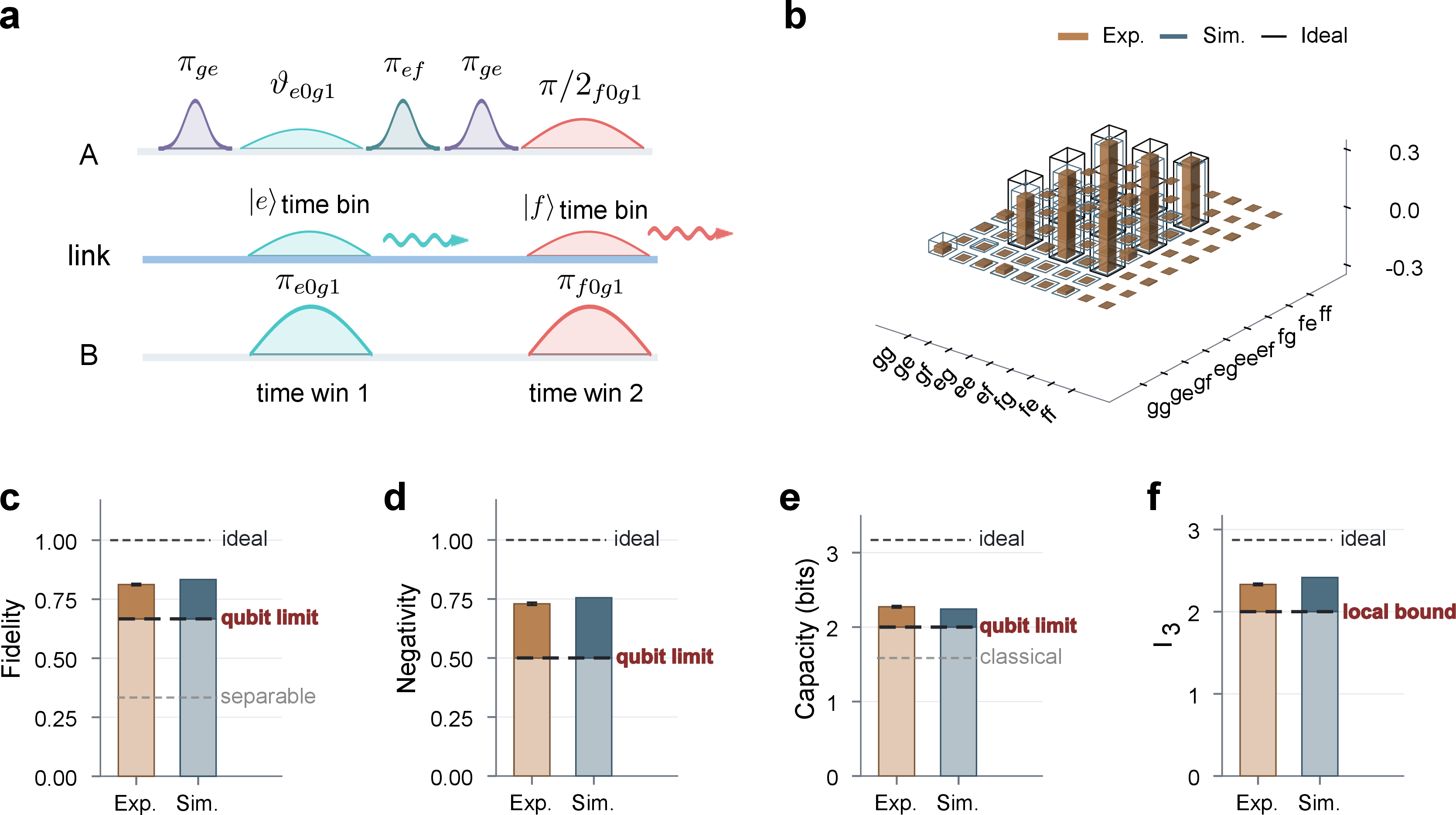
Remote entanglement generation uses the same photon-mediated operations before they reach complete population exchange, but the sequence is a three-path interference protocol rather than two independent partial transfers. Unlike the full-transfer sequence in Fig. 3, the REG sequence starts with the \(e0g1\) branch and then applies the \(f0g1\) branch, because the first operation must split the initial \(\ket{e}_A\) amplitude while leaving a stored component for subsequent relabelling. A partial \(e0g1\) operation first creates one branch that will be absorbed as \(\ket{e}_B\), while the remaining amplitude stays stored in node A. Local \(\pi_{ef}\) and \(\pi_{ge}\) rotations relabel the stored branches, and a subsequent partial \(f0g1\) operation splits the remaining stored amplitude into a no-photon branch and a second-bin photon branch. After full capture, the three coherent alternatives become \(\ket{fg}\), \(\ket{ee}\) and \(\ket{gf}\), giving \((\ket{gf}+\ket{ee}+\ket{fg})/\sqrt{3}\) up to local phases. Because the flying state contains the vacuum, a first-bin photon or a second-bin photon, but no \(\ket{1_1 1_2}\) two-photon component, at most one photon is exposed to propagation loss in the link. The two-qutrit state is reconstructed from the tensor product of the single-qutrit tomography settings, giving 81 joint analysis settings. The density matrix in Fig. 4 contains the corresponding experimental and simulated reconstructions, with \(D(\rho,\rho_{\rm sim})=0.119\). The three target populations and the three pairwise coherences dominate the reconstruction, which is the signature of a coherent two-qutrit Bell state rather than an incoherent mixture of transferred populations.

The state fidelity is \(81.21 \pm 0.37\%\). This exceeds the maximum overlap \(2/3\) between the target maximally entangled qutrit state and any Schmidt-rank-two state, and therefore witnesses Schmidt number 3 [36]. The ensemble-averaged density matrix gives a negativity of \(0.730 \pm 0.005\), above the two-qubit maximum \(0.5\) [37]–[39]. All quoted REG metrics use independently calibrated readout-assignment corrections; their robustness to assignment-matrix uncertainty is quantified in the Supplementary Information. We then evaluate the communication metrics of the same averaged reconstructed state [3]–[6]. The tomography-inferred dense-coding capacity is \(2.273 \pm 0.014\) bits, larger than both the classical qutrit value \(\log_2 3=1.585\) bits and the ideal qubit dense-coding limit of 2 bits. The tomography-inferred CGLMP parameter is \(I_3=2.332 \pm 0.012\), above the local realistic bound. Using the same averaged-density-matrix convention, the corresponding simulated values are \(F=0.834\), \({\cal N}=0.756\), \(C=2.242\) bits and \(I_3=2.417\). This fixed-parameter simulation is used as a consistency check of the reconstructed state structure rather than as a fitted upper bound on the REG benchmarks. These four quantities probe different aspects of the same reconstructed state: overlap with a rank-three target, entanglement dimensionality, communication capacity and nonlocal-correlation strength.

6 Discussion and Conclusion↩︎

The experiment demonstrates coherent qutrit-state transfer and remote qutrit entanglement between two separately packaged superconducting nodes. The central control problem is not simply to increase the local Hilbert-space dimension, but to expose that Hilbert space to a travelling channel one transition at a time. The tunable Purcell filters set the radiative linewidths of the auxiliary resonators, while the transmon flux biases set their dressed frequencies. This combination lets the \(e0g1\) and \(f0g1\) photons occupy the same directional channel, with matched bandwidths and a stable relative phase. A pulse-level cascaded master-equation model, using measured relaxation, internal resonator loss, finite channel efficiency and \(T_1\)-corrected quasi-static \(1/f\)-like detuning noise, reproduces the measured population dynamics and gives the scale of the tomography benchmarks.

The auxiliary resonator is the element that makes this qutrit mapping selective. The quantum state is stored in the transmon levels, while the auxiliary resonator is turned into an itinerant-photon interface only for the addressed transition. The \(e0g1\) pulse opens the \(\ket{e,0}\leftrightarrow\ket{g,1}\) manifold and leaves the \(\ket{f}\) amplitude stored; the \(f0g1\) pulse opens the \(\ket{f,0}\leftrightarrow\ket{g,1}\) manifold and leaves the \(\ket{e}\) amplitude stored. The two non-ground qutrit amplitudes are therefore converted into two separated temporal modes of the same microwave channel. In a direct transmon–waveguide geometry, opening the radiative channel would expose all allowed transitions to the continuum at once, making this time-windowed qutrit encoding difficult without additional filtering. The present architecture separates memory, transition selection and waveguide coupling into different physical elements.

This selectivity is not tied to a single implementation of the sideband interaction. In the present device, the \(e0g1\) primitive is activated by flux modulation of a tunable transmon, and the \(f0g1\) primitive is implemented as a cavity-assisted Raman process. More generally, the same logical operation only requires a controllable sideband between a chosen qutrit transition and the transmission resonator. Such sidebands can also be driven in fixed-frequency circuits, where an off-resonant microwave drive stimulates shaped photon emission at a tunable photon frequency without changing the circuit parameters [55]. Thus the protocol is not tied to flux-tunable transmons: fixed-frequency processors could implement the same time-bin qutrit link if the two qutrit transitions can be coupled selectively to shaped emission and capture, with a calibrated relative phase between the two time bins.

The evidence for operation beyond the qubit limit appears at three levels. First, the average transferred-state fidelity exceeds both the classical qutrit benchmark and the best possible average fidelity of a two-dimensional channel used to transmit an arbitrary qutrit. Second, the generated two-qutrit state has a negativity above the two-qubit maximum, and its target-state fidelity witnesses Schmidt number 3. Third, the same density matrix gives a tomography-inferred dense-coding capacity above the ideal qubit limit and a tomography-inferred CGLMP value above the local realistic bound. These benchmarks test different failure modes: loss of qutrit coherence during transfer, collapse of the entangled state into a two-dimensional subspace, and loss of the information advantage expected from a high-dimensional resource.

The dense-coding and CGLMP numbers should be read in this calibrated-tomography sense. They are not yet a direct dense-coding experiment or a loophole-free Bell test. They show, instead, that the generated density matrix has the structure needed for those protocols. From one maximally entangled qutrit pair, local qutrit gates on the sender side generate the nine orthogonal generalized Bell states \(\{(X^mZ^n\otimes I)\ket{\Phi_3}\}_{m,n=0}^{2}\), with \(\ket{\Phi_3}=(\ket{00}+\ket{11}+\ket{22})/\sqrt{3}\). The inferred capacity therefore quantifies how close the present state is to a usable three-level dense-coding resource. Likewise, the CGLMP value identifies the measurement basis and state quality required for a future direct high-dimensional Bell experiment. Loophole-free Bell tests with remote superconducting qubits have already been realized [15]; the present experiment indicates how such an architecture could be extended from a two-outcome CHSH setting to a three-outcome qutrit measurement. At the current operating point the dominant limitations are finite channel efficiency, qutrit relaxation and low-frequency phase noise, while internal transmission-resonator loss gives a smaller but systematic contribution. Higher channel efficiency, longer qutrit coherence, reduced low-frequency phase noise and improved REG waveform design should therefore increase both the transfer fidelity and the dense-coding capacity.

This conclusion is supported by the simulation error budget and by forward simulations using improved waveform choices in the full cascaded transmission-resonator model, as detailed in the Supplementary Information. Under projected device parameters \(\eta_c=0.98\), \(T_1=50~\mu{\rm s}\) for both addressed qutrit transitions, Markovian \(T_\phi=20~\mu{\rm s}\), and no additional internal transmission-resonator loss, an unwindowed sech emission-and-capture pulse, \(g(t)=g_0/\cosh[(t-t_0)/\tau]\) with \(g_0/2\pi=1/(2\pi\tau)=5~{\rm MHz}\), gives a mean qutrit-transfer state fidelity of \(0.968\) and a qutrit process fidelity of \(0.948\) in the pulse-level model. For REG, the corresponding waveform is obtained from the finite-resonator input-output equations by choosing a smooth emitted mode and solving for the capture controls, with the receiver control allowed to enter the capture window at finite coupling. A representative \(200~{\rm ns}\) REG waveform constrained to \(g_{\rm max}/2\pi=3.95~{\rm MHz}\) under the same projected device parameters gives a REG state fidelity of \(0.939\), negativity \(0.909\), tomography-inferred dense-coding capacity \(2.718\) bits and tomography-inferred \(I_3=2.688\). These projected values remain above the Schmidt-rank-two, two-qubit, dense-coding and local bounds with substantial margins, indicating that improved channel efficiency, longer qutrit coherence and REG waveform optimization would move the platform from a proof-of-principle high-dimensional link toward a higher-fidelity qutrit-network primitive.

The protocol increases the transmitted Hilbert-space dimension without adding another physical link. The same principle can be extended to higher transmon levels, to cavity-encoded qudits, or to multi-node microwave networks in which high-dimensional entanglement is distributed as a resource for modular gates and communication. The key requirement is a matched, tunable interface that can release and absorb different logical amplitudes in controlled temporal modes, while keeping the unused amplitudes protected in a local memory.

7 Methods↩︎

7.1 Device and microwave-link configuration↩︎

Each node consists of a flux-tunable transmon qutrit, an auxiliary resonator for photon emission and capture, a readout resonator, and a tunable Purcell-filter interface to the waveguide. The two nodes are mounted in separate sample boxes and connected by a one-metre microwave cable. The asymmetric-junction transmons provide a broad frequency tuning range while retaining the lowest three levels as the qutrit manifold. The auxiliary-resonator frequency is adjusted through the transmon-induced dispersive Lamb shift, and the external coupling rate is adjusted through the Purcell-filter bias. The sample layout, cryogenic wiring and device parameters are given in Supplementary Figs. S1–S3 and Supplementary Table S1.

7.2 Frequency and linewidth matching↩︎

Efficient photon-mediated transfer requires both frequency matching and bandwidth matching between the two remote interfaces. We first use cavity spectroscopy to track the flux-dependent auxiliary-resonator frequencies of the two nodes. Because the spectroscopy background changes with flux, the maps are background corrected line by line before ridge extraction. The final transfer frequency is determined from matched line cuts and lies near \(7.4347~{\rm GHz}\). The smooth curves in Supplementary Fig. S4 are used only as visual guides for the flux-dependent cavity trajectories and are not used to define the final operating frequency.

The Purcell-filter control is calibrated by preparing one photon in the auxiliary resonator and measuring the cavity-energy decay as a function of the filter \(z\)-pulse amplitude. Each trace is fitted to \[P_1(t)=P_{\rm off}+A\exp(-t/T_{\rm cav}),\] and the loaded coupling decay rate is reported as \[\kappa/2\pi=\frac{1}{2\pi T_{\rm cav}}.\] The nearest directly measured high-bandwidth settings used in the experiment are \(z_A=0.37\), giving \(\kappa_A/2\pi=10.72\pm0.44~{\rm MHz}\), and \(z_B=0.21\), giving \(\kappa_B/2\pi=10.28\pm0.26~{\rm MHz}\). The full linewidth calibration, including the finite square-pulse response at the largest coupling settings, is shown in Supplementary Fig. S5.

7.3 Parametric transfer primitives↩︎

The elementary transfer primitives are implemented with flux-parametric modulation of the qutrit-resonator interaction. The \(e0g1\) pulse couples \(\ket{e,0}\) and \(\ket{g,1}\), while the \(f0g1\) pulse couples \(\ket{f,0}\) and \(\ket{g,1}\). The emitted photon from node A propagates through the directional microwave channel and is captured by the corresponding pulse on node B. The pulses have a \(200~{\rm ns}\) sine amplitude envelope in the experiment. This envelope is used as a practical photon-shaping pulse: it produces an approximately time-symmetric itinerant mode for matched emission and capture, while avoiding the abrupt spectral components of a square pulse. The sender pulse defines the start of the primitive. The receiver pulse starts \(8~{\rm ns}\) after the sender pulse for \(e0g1\) and \(13~{\rm ns}\) after the sender pulse for \(f0g1\), compensating the propagation delay and the calibrated temporal offset between emission and absorption. All measured populations in Fig. 2 are compared at the same physical cutoff time. For a full primitive, the pulse amplitudes are set near the first maximum of the transfer population. In the small-amplitude regime used for partial primitives, the \(e0g1\) flux-drive amplitude and the \(f0g1\) Raman-drive amplitude are proportional to the corresponding effective resonant coupling strengths, so reducing the programmed amplitude reduces the pulse area and stops the exchange at the desired population splitting.

The microwave frequency is chirped during each primitive pulse. For \(e0g1\), the flux-parametric modulation changes the average transmon frequency during the pulse, so a fixed modulation frequency would move away from the instantaneous sideband resonance. For \(f0g1\), the cavity-assisted Raman drive produces an amplitude-dependent ac Stark shift. We calibrate these shifts by sweeping pulse amplitude and drive frequency for each node and primitive, extracting the resonance ridge, and converting the calibrated ridge into an instantaneous frequency program \(\omega_d[A(t)]\) for the sine envelope. The pulse-level simulations are evaluated in this chirp-corrected resonant frame; residual detuning is included through the measured slow-dephasing model.

For the primitive population and two-level QPT data, the measured levels are chosen according to the addressed subspace. In the \(f0g1\) primitive, an additional calibrated \(\pi_{ef}\) mapping pulse is applied before readout when the analysis is performed in the \(\{\ket{g},\ket{e}\}\) readout basis. This mapping does not change the physical transfer primitive; it only maps the receiver \(\ket{f}\) population to a level that is read out with higher contrast in that calibration.

7.4 Qutrit state transfer and entanglement sequences↩︎

Arbitrary qutrit-state transfer is obtained by applying the two primitive transfer operations to the non-ground components of the input state. Each experimental run starts with both nodes reset to \(\ket{g}\). A local preparation sequence on node A generates one of the qutrit input states used for QST or QPT, while node B remains in \(\ket{g}\). The transfer sequence then applies the two time-delayed sender-receiver pulse pairs. In the sequence used for Fig. 3, the \(f0g1\) pair is applied first and transfers the \(\ket{f}_A\) amplitude through the first time bin; the \(e0g1\) pair is applied second and transfers the \(\ket{e}_A\) amplitude through the second time bin. The \(\ket{g}_A\) component is not resonant with either primitive and remains the two-bin vacuum component of the transfer channel. The ideal transfer maps \[\alpha\ket{g}_A+\beta\ket{e}_A+\gamma\ket{f}_A \rightarrow \alpha\ket{g}_B+\beta e^{i\phi_e}\ket{e}_B+\gamma e^{i\phi_f}\ket{f}_B,\] where the phases \(\phi_e\) and \(\phi_f\) are removed by calibrated virtual-\(Z\) rotations. The input states used for qutrit process tomography are generated by local qutrit rotations in the \(\ket{g}\)-\(\ket{e}\) and \(\ket{e}\)-\(\ket{f}\) subspaces. The tomography procedure, readout correction and basis convention are described in the Supplementary Information.

Remote entanglement generation uses partial transfer operations derived from the same \(e0g1\) and \(f0g1\) primitives. The experiment again starts from node B initialized in \(\ket{g}\), while node A is locally prepared for the entangling sequence. In the ideal lossless map, a local \(\pi_{ge}\) pulse prepares \(\ket{e}_A\). An \(e0g1\) partial-transfer pulse with angle \(2\arctan(1/\sqrt{2})\) creates a \(1/\sqrt{3}\) first-bin photon branch and a \(\sqrt{2/3}\) stored branch. Local \(\pi_{ef}\) and \(\pi_{ge}\) rotations then relabel the stored branches, and a subsequent \(f0g1\) partial-transfer pulse with angle \(\pi/2\) divides the remaining stored amplitude into a no-photon branch and a second-bin photon branch. The receiver uses full \(e0g1\) and \(f0g1\) capture pulses to map the first and second time bins to \(\ket{e}_B\) and \(\ket{f}_B\), respectively. The calibrated experimental pulse amplitudes and virtual-\(Z\) phases implement the same three-path interference condition after accounting for loss, finite capture efficiency and phase accumulation. The sequence is calibrated to generate the target state \[\ket{\Psi_{\rm qutrit}}=\frac{1}{\sqrt{3}}\left(\ket{gf}+\ket{ee}+\ket{fg}\right),\] up to local phases. The local \(ef\)-frame corrections applied before reporting the density matrix are \(0.911~{\rm rad}\) on node A and \(-2.035~{\rm rad}\) on node B. Additional tomography phase diagnostics and robustness checks are shown in Supplementary Figs. S10 and S11.

7.5 Qutrit tomography and readout correction↩︎

Qutrit state tomography is performed by applying a tomographically complete set of analysis rotations before three-state readout [26], [56], [57]. For a single qutrit, we use nine analysis settings that map the populations and the real and imaginary parts of the \(\ket{g}\)-\(\ket{e}\), \(\ket{g}\)-\(\ket{f}\) and \(\ket{e}\)-\(\ket{f}\) coherences onto measured three-level populations. For two-qutrit tomography, the same single-qutrit analysis set is applied independently to both nodes, giving \(9\times9\) joint analysis settings and nine three-state joint readout outcomes for each setting. In the main tomography datasets, each probability for a given analysis setting is obtained from 4000 single-shot repetitions. The explicit analysis rotations are listed in the Supplementary Information.

For each measured qutrit, the readout assignment matrix \(M\) is independently calibrated, with elements \(M_{ij}=P({\rm measured}\;i|{\rm prepared}\;j)\). For two-qutrit tomography, the full readout matrix is taken as the tensor product of the independently calibrated single-qutrit assignment matrices. The measured probability vector \(p_{\rm meas}\) is corrected by \[p_{\rm corr}=M^{-1}p_{\rm meas}.\] The density matrix is then obtained from the corrected tomography probabilities by maximum-likelihood estimation with unit-trace and positive-semidefinite constraints. The readout matrices used for the data in Figs. 3 and 4 are shown in Supplementary Fig. S8. Unless otherwise specified, the fidelities and density matrices reported in the main text are readout corrected.

7.6 Process tomography and benchmark definitions↩︎

For qutrit process tomography, we prepare nine linearly independent qutrit input states on node A, transfer each state through the microwave link, and reconstruct the corresponding output density matrix on node B with qutrit state tomography. The input set is generated from \(\ket{g}\) by calibrated rotations in the \(ge\) and \(ef\) subspaces, and spans the three populations and the three pairwise coherences of the qutrit. The same analysis is applied to the input states in separate calibration runs to account for state-preparation imperfections. The input-output density-matrix pairs are then used to infer the process matrix \(\chi\) in the Gell-Mann basis [52], [53]. The process fidelity is calculated as \[F_{\chi}={\rm Tr}\left(\chi_{\rm exp}\chi_{\rm ideal}\right),\] with both process matrices represented in the same basis and normalization convention. The transferred-state fidelity is calculated between the reconstructed output state and the corresponding ideal target state. The mean state fidelity is the average over the tested input states.

The classical qutrit benchmark used for state transfer is \(F_{\rm cl}=1/2\), corresponding to the optimal measure-and-prepare strategy for an unknown qutrit state [34]. The qubit-channel benchmark is \(F_{\rm qb}=3/4\), the maximum average fidelity for transmitting an arbitrary qutrit through an effective two-dimensional quantum channel [35]. These bounds are used only for the full qutrit-transfer channel, not for the primitive two-level transfer processes.

7.7 Entanglement metrics and dense-coding capacity↩︎

The two-qutrit state fidelity is calculated with respect to \(\ket{\Psi_{\rm qutrit}}\) using the standard state-fidelity convention [58]. The negativity is computed from the partial transpose of the reconstructed density matrix [37], [38], \[\mathcal{N}(\rho)=\frac{\|\rho^{T_B}\|_1-1}{2}.\] For a maximally entangled qutrit target, any state with Schmidt number at most two has fidelity no larger than \(2/3\) [36]. For any two-qubit state, the maximum negativity is \(0.5\); values above this limit certify entanglement that cannot be represented within a two-qubit Hilbert space.

The dense-coding capacity is evaluated from the reconstructed two-qutrit state as [3]–[5] \[C=\log_2 d+S(\rho_B)-S(\rho_{AB}),\] with local dimension \(d=3\), reduced state \(\rho_B={\rm Tr}_A(\rho_{AB})\), and von Neumann entropy \(S(\rho)=-{\rm Tr}(\rho\log_2\rho)\). We compare this value with the classical qutrit value \(\log_2 3\) and the ideal qubit dense-coding limit of 2 bits. The CGLMP parameter \(I_3\) is calculated from the reconstructed density matrix using the standard two-setting, three-outcome measurement bases [6]. The full convention and basis mapping are provided in the Supplementary Information.

7.8 Cascaded master-equation simulation↩︎

The simulations use a pulse-level cascaded master equation implemented in QuTiP [48]–[51]. The model includes the qutrit degrees of freedom of both nodes, the auxiliary resonator modes, the directional coupling between the two nodes, internal resonator loss, channel transmission efficiency and qutrit relaxation. The channel efficiency and internal-loss parameters used for the main figures are \[\begin{align} \eta_c&=0.92,\\ \kappa_{{\rm int},A}/2\pi=0.0208~{\rm MHz},&\qquad \kappa_{{\rm int},B}/2\pi=0.0176~{\rm MHz}. \end{align}\]

Dephasing is included as a \(T_1\)-corrected quasi-static \(1/f\)-like detuning ensemble. For each noise realization, the qutrit transition frequencies are shifted by static detunings drawn from Gaussian distributions whose widths are extracted from Ramsey measurements after subtracting the contribution from energy relaxation. The simulated density matrices and populations are averaged over the detuning ensemble. This treatment captures the slow dephasing that dominates the experiment without overestimating the loss of coherence during the \(200~{\rm ns}\) transfer pulses. The model uses fixed calibrated parameters during each tomography simulation and does not include additional drift of the transfer resonance or readout assignment matrix. The detailed Hamiltonian, collapse operators, noise extraction, \(1/f\)-versus-Markovian noise comparison and sine-versus-sech pulse comparison are given in the Supplementary Information.

7.9 Uncertainties↩︎

Error bars in the population-dynamics data are obtained from repeated measurements and grouped dataset averages. Error bars for state and process fidelities are calculated from repeated tomography reconstructions. For the Purcell-filter linewidth calibration, the uncertainty in \(T_{\rm cav}\) is taken from the covariance matrix of the single-exponential fit and propagated to \(\kappa/2\pi\) using \[\delta(\kappa/2\pi)=\frac{\delta T_{\rm cav}}{2\pi T_{\rm cav}^2}.\]

Supplementary information↩︎

Supplementary Information accompanies this manuscript. It includes the sample layout, measurement-chain schematic, device parameters and readout matrices, cavity spectroscopy, Purcell-filter linewidth calibration, chirped-pulse calibration, primitive transfer delay and phase scans, primitive tomography diagnostics, tomography phase diagnostics, readout-correction checks, the cascaded master-equation derivation, the \(1/f\)-dephasing model, the dense-coding and CGLMP conventions, the waveform comparison, the inverse-designed REG waveform construction, and the simulation error budget.

data availability statement↩︎

The data produced in this work is available from the corresponding authors upon reasonable request.

author contributions↩︎

D.-N.Z., H.F and X.L. supervised the project. X.L. conceived the idea. X.L., Y.-J.L and Z.-Y.M designed the sample. X.L. performed the experiment, processed the data and wrote this manuscript. Z.-Y.M fabricated the sample. Y.H. and S.-L.Z helped with several iterations of the sample. All authors contributed to the discussions and production of the manuscript.

competing interests↩︎

The authors declare no competing interests.

References↩︎