Resonant Brane Splatting for Arbitrary-Scale Super-Resolution
January 01, 1970
Abstract
Arbitrary-Scale Super-Resolution (ASR) reconstructs images at continuous magnification factors. Recent methods accelerate inference by replacing computationally heavy implicit neural decoders with explicit 2D Gaussian Splatting (GS). However, since standard Gaussians are smooth low-pass primitives, modeling edges and fine textures requires multiple overlapping, well-aligned splats, which creates severe bottlenecks during rasterization. To address this, we introduce Resonant Brane Splatting (RBS), a feed-forward ASR framework. RBS replaces flat Gaussians with Branes: expressive primitives that emit spatially varying colors to natively model local contrast and complex textures within a single footprint. We achieve this by augmenting the standard Gaussian envelope with internal Gaussian-Hermite modes, assigning a distinct color coefficient to each. The zero-order mode recovers standard GS, while higher-order modes capture high frequencies. We predict Brane parameters directly from low-resolution features. Because Branes provide a mathematically richer formulation than simple Gaussians, far fewer primitives need to overlap to reconstruct a given target pixel. To exploit this, we introduce an efficient fully differentiable rasterizer with a precise culling strategy based on the classical quantum turning point. This allows us to safely skip negligible regions, drastically reducing the rendering overhead. Experiments on standard ASR benchmarks show that RBS improves reconstruction quality over implicit and GS baselines, while achieving superior speed-quality trade-off than prior GS methods.
1 Introduction↩︎
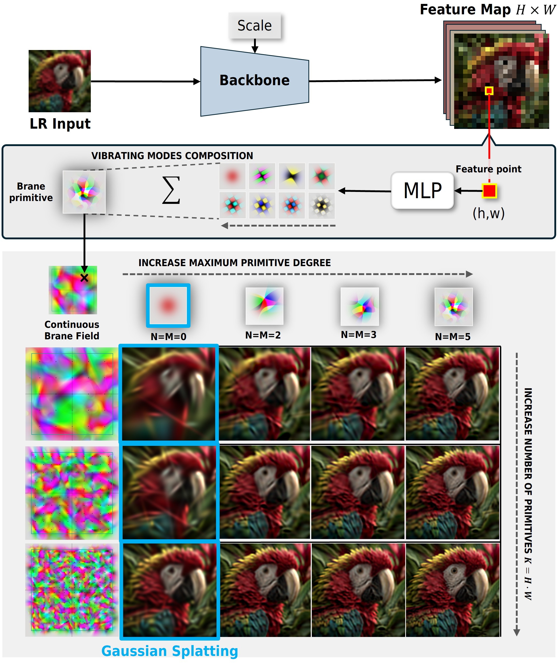
Image Super-Resolution (SR) recovers details from low-resolution (LR) inputs, while Arbitrary-Scale SR (ASR) extends this goal to continuous magnification factors. Implicit Neural Representations (INRs) [1]–[7] dominated ASR by learning coordinate-to-color mappings. While flexible, INRs require dense pixel-wise queries at inference time and suffer from spectral bias, making high frequencies difficult to reconstruct faithfully.
Recent 2D Gaussian Splatting (GS) methods [8], [9] replace implicit decoding with explicit rendering, predicting primitives from LR features. While efficient, a standard Gaussian remains a smooth, low-pass footprint limited to a single color. Because a single Gaussian cannot represent internal color variations, modeling sharp edges or complex textures forces the network to rely on the precise alignment and collaboration of numerous overlapping splats. This high degree of overlap creates a severe bottleneck, directly slowing down the rasterization process.
To name our proposed 2D splatting framework for ASR (Fig. 1), we draw a purely conceptual analogy from M-Theory [10]. In this theory, vibrating multidimensional p-branes [11] (generalizing strings [12]) form particles that aggregate into macroscopic matter. While this remains a metaphorical inspiration, our Brane primitive adopts the exact mathematical eigenfunctions of the Quantum Harmonic Oscillator [13]. By augmenting a Gaussian envelope with internal Gaussian-Hermite modes, our primitive mathematically “vibrates” to create local structural patterns. Ultimately, the aggregation of these patterns constructs the complex visual matter of the super-resolved image.
While prior work applied Gaussian-Hermite functions to spatial support [14] on 3D tasks, we uniquely use this basis for appearance generation. By assigning distinct color coefficients to each mode, a single Brane natively emits spatially varying colors. The zero-order mode recovers standard Gaussian splatting, while higher-order modes model signed color residuals. A single Brane can therefore synthesize local contrast, sharp edges, and multi-colored textures, representing high-frequency patterns with fewer splats. A feed-forward network predicts Brane parameters directly from LR features. Since Branes internally model complex textures, dense primitive overlapping is no longer required. To maximize inference speed, we design a custom differentiable CUDA rasterizer that bounds primitive evaluation using the quantum turning point, the exact radial threshold before Gaussian-Hermite modes exponentially decay. Safely culling Branes outside this boundary accelerates rendering well beyond standard GS.
Our contributions are: (i) Resonant Brane Splatting, a Gaussian-Hermite primitive generalizing flat, single-color Gaussians into structured, color-generating splats; (ii) a feed-forward ASR framework predicting Brane geometry, opacity and mode-wise color coefficients from LR features; (iii) a differentiable 2D GPU/CUDA-based scale-aware rasterizer exploiting bounded Gaussian-Hermite support for faster inference; and (iv) state-of-the-art visual performance, establishing a new optimal balance between rendering speed and image quality.

2 Related Work↩︎
2.0.0.1 Image Super-Resolution.
Fixed-scale image Super-Resolution has evolved from early CNNs [15] to sophisticated architectures leveraging expanded receptive fields [16]–[18], compressed feature spaces [19], and Residual-in-Residual structures [20]–[23]. Transformer models [24]–[26] further improved long-range dependency modeling. While diffusion models excel in perceptual SR, iterative sampling and hallucination risks hinder efficient, faithful reconstruction [27]–[31]. Crucially, these methods require scale-specific training and lack continuous magnification at inference.
2.0.0.2 Arbitrary-Scale SR and Continuous Representations.
ASR breaks integer-scale constraints by framing SR as a continuous representation problem [1], [32]. LIIF [2] formalized this by mapping continuous spatial coordinates to RGB values via an MLP. Subsequent works mitigated spectral bias and improved feature aggregation through Fourier mappings [3], Normalizing Flows [5], implicit attention [6], neural operators [4], and frequency encodings [33], [34]. Because dense point-wise MLP queries create severe inference bottlenecks, LMF [7] confined heavy computation to the LR space. However, coordinate-wise decoding still treats each output pixel independently, limiting data reuse across neighboring pixels and motivating explicit rendering alternatives based on spatial primitives.
2.0.0.3 Splatting-Based ASR.
Recently, 2D Gaussian Splatting (GS) [35] emerged as a faster ASR alternative. GaussianSR [8] blends pre-trained kernels, while GSASR [9] and the lightweight GRAPE [36] predict learnable anisotropic parameters. ContinuousSR [37] explicitly models continuous HR signals in a single pass. However, standard Gaussians inherently act as low-pass footprints requiring strong anisotropy for high-frequency synthesis, limiting local expressiveness and making reconstruction sensitive to splat alignment.
2.0.0.4 Expressive Splatting Primitives.
To overcome GS limitations, recent works in 3D rendering explore modified primitives [38]–[43]. Closely related to our work, 2DGH [14] introduced Gaussian-Hermite kernels for 2D Gaussian splatting in per-scene 3D reconstruction and novel-view synthesis. By modulating Gaussian splats with Hermite series, 2DGH increases the capacity of the kernel to represent sharp boundaries and fine geometric structures during scene optimization.
2.0.0.5 Positioning of our work.
We build on the expressive Gaussian-Hermite primitive but differ in how appearance is represented. In 2DGH [14], the Gaussian-Hermite function defines the spatial opacity/support profile, while color remains a separate splat attribute. In contrast, we assign an RGB-valued coefficient to each Hermite mode, so the color emitted by a Brane varies according to its internal modes rather than being constant over the primitive. This allows a single primitive to model local contrast, structure, and multi-colored texture within the same footprint, instead of relying on stretched shapes or multiple overlapping splats to approximate high-frequency details.
3 Method↩︎
3.1 Limitations of Splatting-Based ASR↩︎
Given a low-resolution input image \(\mathbf{I}_{LR} \in \mathbb{R}^{H \times W \times 3}\) and a continuous target scale factor \(s \in \mathbb{R}^{+}\), Arbitrary-Scale Super-Resolution predicts an output image \(\mathbf{I}_{SR} \in \mathbb{R}^{H_\text{SR} \times W_\text{SR} \times 3}\) with \(H_\text{SR} = \lfloor Hs \rfloor\) and \(W_\text{SR} = \lfloor Ws \rfloor\). We follow the splatting-based ASR framework of [9]: a neural backbone extracts a dense feature map \(\hat{\mathbf{F}}\in\mathbb{R}^{\hat{H} \times \hat{W} \times C}\). To increase its spatial density, it can be optionally upsampled by a factor \(u\in\mathbb{N}^{+}\), obtaining \(\mathbf{F}\in\mathbb{R}^{H' \times W' \times C}\), with \(H'=u\hat{H}\) and \(W'=u\hat{W}\). Each feature vector in \(\mathbf{F}\) predicts one spatial primitive to be rendered at the target resolution. Let \(K=H'W'\) be the number of primitives and let \(\mathbf{f}_k \in \mathbb{R}^{C}\) denote the feature associated with the \(k\)-th grid cell. Each primitive is anchored in the normalized image domain \([0,1]^2\) and contributes to the final color \(\mathbf{C}(u,v)\) of a target pixel \((u,v)\) through explicit rasterization. In standard Gaussian splatting, \[\mathbf{C}(u,v) = \sum_{k=1}^{K} \alpha_k E(x'_k,y'_k)\mathbf{c}_k\,, \label{eq:gs95primitive}\tag{1}\] where each primitive \(k\) has a single color vector \(\mathbf{c}_k \in [0,1]^3\), an opacity \(\alpha_k\), a Gaussian spatial envelope \(E(x,y)=\exp\left(-\frac{1}{2}(x^2+y^2)\right)\) computed at the local canonical coordinates \((x'_k,y'_k)\) of pixel \((u,v)\).
This formulation is efficient, but the primitive is locally limited: the color is constant over the footprint and all high-frequency structure must be explained through geometry and overlap with neighboring splats.
3.2 Resonant Brane Primitive↩︎
To overcome this bottleneck, we replace each flat Gaussian splat with a Resonant Brane. A Brane keeps the Gaussian envelope of Eq. 1 , but augments it with internal Gaussian-Hermite modes. Just as these modes describe the localized vibrational states of a Quantum Harmonic Oscillator [13], they define higher-order polynomial patterns inside the exact same spatial support. This allows the primitive to represent complex internal structure instead of behaving as a flat, single-color footprint.
We define the Brane in a local 2D canonical space. The spatial boundary is governed by the same Gaussian envelope \(E(x,y)\). Inside this envelope, we use normalized Hermite polynomials [44] \[\begin{align} \bar{H}_n(z) &= \frac{1}{\sqrt{2^n n!}} H_n(z), \quad \text{where}\\ H_0(z) &= 1, \qquad H_1(z)=2z, \quad \text{and} \\ H_n(z) &= 2zH_{n-1}(z)-2(n-1)H_{n-2}(z)\,\text{ for }\,n>1\,. \\ \end{align} \label{eq:normalized95hermite95recurrence}\tag{2}\] Here, \(H_n(z)\) is the physicist’s Hermite polynomial of degree \(n\), that can be computed efficiently via the above recursive relation [45]. The normalization removes the dominant degree-dependent growth of \(H_n\), improving numerical stability when using higher-order modes.
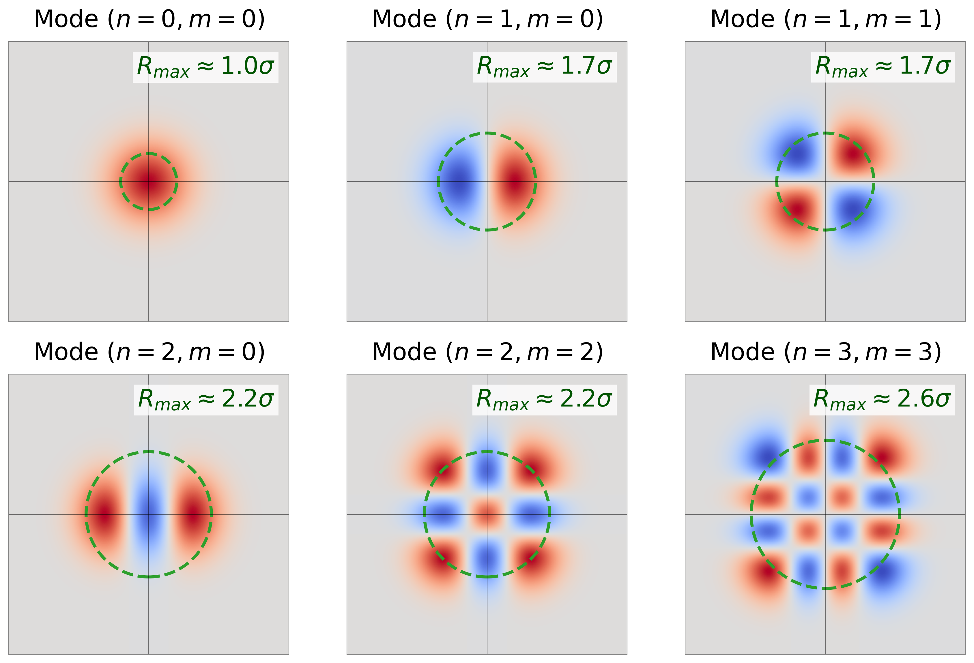
Local 2D variations inside the Gaussian envelope can be expressed by combining one-dimensional Hermite modes along the canonical axes. A 2D mode of degree \((n,m)\) is given by the tensor product \[\Psi_{n,m}(x,y)=\bar{H}_n(x)\bar{H}_m(y)\,. \label{eq:hermite95mode}\tag{3}\] Figure 3 shows 2D modes when varying the degree \((n,m)\).
Gaussian-Hermite functions have already been used in splatting to make the spatial support (i.e., the shape of the opacity kernel) more expressive than an ellipse [14]. We use the same modal basis but to model appearance. Instead of assigning one color to the whole primitive, we assign its own color coefficient \(\mathbf{c}_{n,m} \in \mathbb{R}^3\) to each mode. The Brane emission is therefore \[\mathcal{B}(x,y) = \alpha E(x,y) \sum_{n=0}^{N} \sum_{m=0}^{M} \mathbf{c}_{n,m}\Psi_{n,m}(x,y) \,. \label{eq:brane95definition}\tag{4}\] This makes a Brane a color-generating primitive. The zero-order mode (\(N=M=0\)) gives \(\mathcal{B}(x,y) = \alpha E(x,y) \mathbf{c}_{0,0}\), which is exactly a standard Gaussian splat. Higher-order modes instead act as signed color residuals. They can add or subtract color locally inside the same footprint, allowing one primitive to synthesize local contrast, edges, and multi-colored textures without decomposing them into many small or highly anisotropic Gaussians (Fig. 2).
3.3 Predicting Branes from LR Features↩︎
We now map the Brane primitive to ASR. The feature grid \(\mathbf{F}\) defines \(K=H'W'\) Branes over the normalized image domain. For each feature vector \(\mathbf{f}_k\), the network predicts the full Brane state \[\Phi_k = \left[ \begin{array}{c@{\;}c@{\;}c} \underbrace{\Delta x_k,\Delta y_k}_{\text{anchoring}}, & \underbrace{\sigma_{x,k},\sigma_{y,k},\rho_k,\alpha_k}_{\text{footprint \& opacity}}, & \underbrace{\mathbf{c}_{0,0,k},\ldots,\mathbf{c}_{N,M,k}}_{\text{mode colors}} \end{array} \right]. \label{eq:brane95parameters}\tag{5}\]
Geometric anchoring. The \(k\)-th Brane is initially anchored at the center of its feature grid cell \[(x^{\text{ref}}_k,y^{\text{ref}}_k) = \left( \frac{j+0.5}{W'}, \frac{i+0.5}{H'} \right).\] To allow sub-pixel adaptation, an MLP head predicts continuous offsets \[(\Delta x_k,\Delta y_k)=\operatorname{MLP}_{\theta_1}(\mathbf{f}_{k})\,,\] yielding the final center \((x_k, y_k)\) as \[x_k=x^{\text{ref}}_k+\frac{\Delta x_k}{W'}\,, \qquad y_k=y^{\text{ref}}_k+\frac{\Delta y_k}{H'}\,.\]
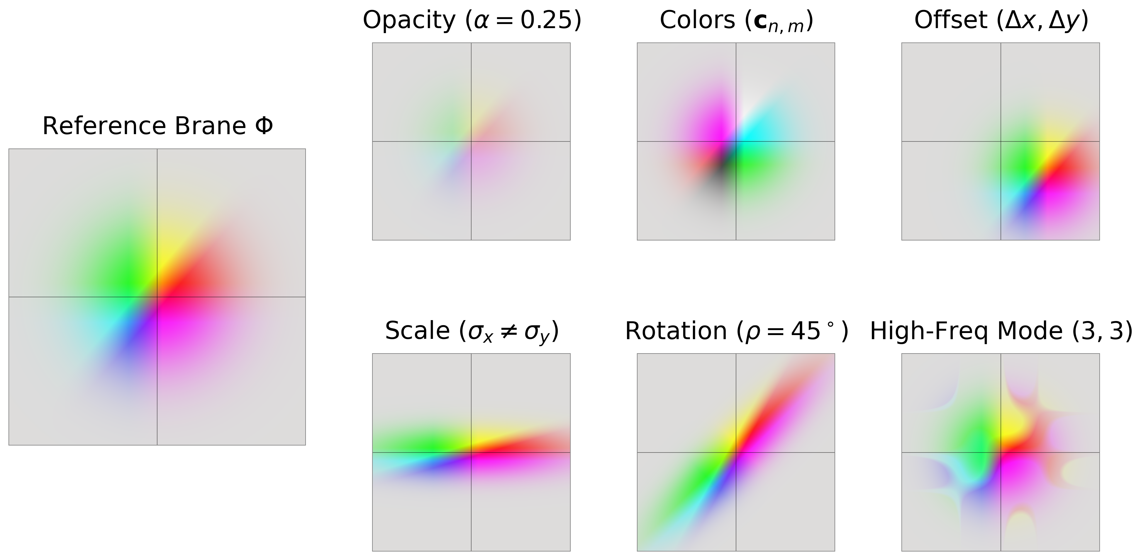
Footprint and opacity. Additional heads predict the anisotropic scales, rotation, and opacity as \[\begin{align} (\sigma_{x,k},\sigma_{y,k}) &= \operatorname{sigmoid}(\operatorname{MLP}_{\theta_3}(\mathbf{f}_{k})),\\ \rho_k &= \pi\,\operatorname{tanh}(\operatorname{MLP}_{\theta_4}(\mathbf{f}_{k})),\\ \alpha_k &= \operatorname{sigmoid}(\operatorname{MLP}_{\theta_5}(\mathbf{f}_{k})). \end{align}\] Figure 4 shows the effect of parameters on appearance.
Mode colors. Given maximum degrees \(N\) and \(M\), each Brane has \(L=(N+1)(M+1)\) modes. A dedicated head predicts all raw mode colors \[\tilde{\mathbf{C}}_k = \operatorname{MLP}_{\theta_2}(\mathbf{f}_{k}) \in \mathbb{R}^{3L}.\] We reshape this vector into \(L\) color coefficients \(\tilde{\mathbf{c}}_{k}^{n,m}\in\mathbb{R}^3\). The zero-order coefficient is constrained to a positive color range, while higher-order modes are signed residuals: \[\mathbf{c}_{k}^{n,m} = \begin{cases} \operatorname{sigmoid}(\tilde{\mathbf{c}}_{k}^{n,m}) , & n=0,\;m=0,\\ \operatorname{tanh}(\tilde{\mathbf{c}}_{k}^{n,m}) , & \text{otherwise}. \end{cases} \label{eq:mode95color95activation}\tag{6}\] Thus, \(\mathbf{c}^{0,0}_{k}\) defines the smooth base color, while higher-order coefficients can add or subtract color inside the footprint.
3.4 Differentiable Rasterization↩︎

To render the output image, each target pixel \((u,v)\) is first projected into normalized coordinates \[(u_{\text{norm}},v_{\text{norm}}) = \left( \frac{u+0.5}{W_\text{SR}}, \frac{v+0.5}{H_\text{SR}} \right).\] For the \(k\)-th Brane, we compute the displacement from its center as \[(\delta x_k,\delta y_k) = (u_{\text{norm}}-x_k,\;v_{\text{norm}}-y_k)\] that is then mapped to the local canonical coordinates through inverse rotation and scaling \[\begin{pmatrix} x'_k\\ y'_k \end{pmatrix} = \begin{pmatrix} \frac{1}{\sigma_{x,k}} & 0\\ 0 & \frac{1}{\sigma_{y,k}} \end{pmatrix} \begin{pmatrix} \cos\rho_k & \sin\rho_k\\ -\sin\rho_k & \cos\rho_k \end{pmatrix} \begin{pmatrix} \delta x_k\\ \delta y_k \end{pmatrix}. \label{eq:inverse95transformation}\tag{7}\] The final RGB value \(\mathbf{C}(u,v)\) is obtained by additively splatting all active Branes \[\mathbf{C}(u,v) = \sum_{k=1}^{K} \alpha_k E(x'_k,y'_k) \sum_{n=0}^{N} \sum_{m=0}^{M} \mathbf{c}_{n,m,k} \bar{H}_n(x'_k) \bar{H}_m(y'_k). \label{eq:rbs95rendering}\tag{8}\]
3.4.0.1 Culling Branes.
Dense evaluation across all Branes and pixels requires \(\mathcal{O}(K H_{SR} W_{SR})\) operations. Our CUDA rasterizer (Algorithm 6) avoids this via a dual culling strategy to efficiently determine the final color of each pixel. First, we map the target pixel into the continuous Brane field and define a bounding region around it using \(d_{\max}\), which represents a specific fraction of this normalized space. We restrict our evaluation strictly to the candidate Branes located inside this area. Second, to accelerate rendering further, we filter these surviving Branes by evaluating only those with a meaningful contribution. We achieve this using a canonical space boundary check based on the quantum turning point \(R_{\max} = \sqrt{2n_{\max} + 1}\) [13], that is the radius beyond which the visual impact of a Brane with maximum degree \(n_{\max}=\max{(N,M)}\) is empirically negligible. Thus, we discard candidates where \({x'_k}^2 + {y'_k}^2 > R_{\max}^2\).

4 Experiments↩︎

4.1 Experimental Setup↩︎
4.1.0.1 Implementation details.
To isolate our contribution, we adopt the GSASR [9] pipeline (EDSR [46] or RDN [22] with a Transformer refiner). Replacing only the standard 2D Gaussian projection heads to output the Brane parameters (Eq. 5 ) introduces a strictly negligible parameter overhead, confirming our performance leaps stem directly from the Brane’s structural expressiveness. We default to Hermite degree \(N=M=3\) to maximize the efficiency-effectiveness trade-off. For training on DIV2K [47], given a continuous scale \(s\) and a \(48 \times 48\) LR patch, our CUDA rasterizer renders an SR prediction of size \(\lfloor 48s \rfloor \times \lfloor 48s \rfloor\). The framework is optimized end-to-end by minimizing the \(\mathcal{L}_1\) loss between this prediction and the corresponding ground-truth HR crop. We use Adam for 500k iterations at \(s \sim \mathcal{U}(1, 4)\), with an initial learning rate of \(10^{-4}\) halved every 100k steps, followed by a 50k-iteration fine-tuning at \(s \sim \mathcal{U}(1, 8)\) on three H100 GPUs.
4.1.0.2 Compared models.
We compare RBS against leading implicit models (Meta-SR [1], LIIF [2], LTE [3], SRNO [4], LINF [5], CiaoSR [6], LMF [7]) and explicit splatting-based methods (ContinuousSR [37], GRAPE [36], GaussianSR [8], GSASR [9]).
4.1.0.3 Evaluation protocol.
We test on standard benchmarks (Set5 [48], Set14 [49], DIV2K100 [47], Urban100 [50], BSDS100 [51], Manga109 [52], General100 [53], LSDIR [54]) at standard scales (\(s \in \{2, 3, 4, 6, 8, 12\}\)) and assess out-of-distribution generalization at extreme scales (\(s \in \{16, 18, 24, 30\}\)) on DIV2K100 and LSDIR. Metrics include PSNR/SSIM [55] (Y-channel), LPIPS [56], and DISTS [57], computed using official pre-trained models via unified scripts. Following GSASR [9], we benchmark end-to-end efficiency on a single H100 using fixed \(720^2\) HR center crops from the original DIV2K images. Since this protocol fixes the HR ground-truth size, larger upsampling scales correspond to smaller LR inputs. As a result, backbone cost and, for splatting methods, the number of rasterized primitives decrease with scale, so the reported runtime and memory also tend to decrease.
4.2 Discussion↩︎
4.2.0.1 Reconstruction quality.
Table ¿tbl:tab:urban10095set595edsr? reports results on Urban100 and Set5, while the other benchmarks are provided in Supplementary Material. These datasets represent the two extremes of our evaluation. Urban100 contains abundant high-frequency structures, allowing RBS to fully exploit its higher-order modes and consistently outperform competing methods. In contrast, Set5 is dominated by smooth content that is already well modeled by standard Gaussian primitives, making it the least favorable setting for RBS. Even in this regime, RBS remains competitive with the strongest Gaussian-based approaches. Results on the remaining datasets lie between these two extremes and follow the same overall trend.
4.2.0.2 Representational capacity.
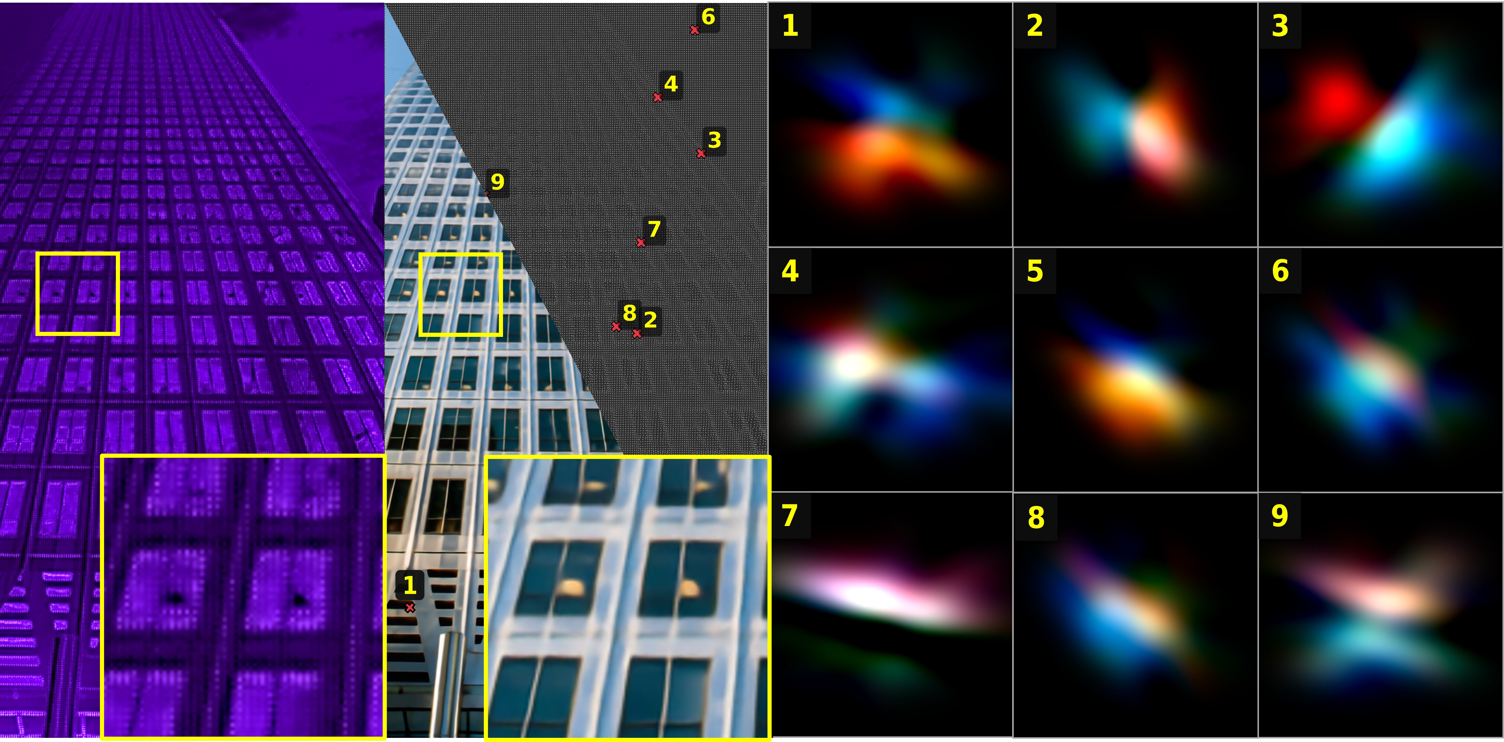
Standard splatting methods [8], [9], [36], [37] require dense overlaps of constant color primitives. Instead, Branes use Hermite modes to independently model complex textures (Fig. 9). Consequently, RBS remains highly competitive even when aggressively reducing the primitive count (see the no up and \(\times 2\) configurations in Table 2). This representational power is spatially adaptive, activating higher modes at complex edges while regressing to standard Gaussians in flat regions (Figs. 7, 8).
4.2.0.3 Efficiency versus density.
In Table 1, implicit models appear highly efficient because they evaluate only one query per target pixel. Explicit splatting methods can match this minimal overhead when using one primitive per LR pixel, as shown by the no-up setting in Table 2. However, high reconstruction quality typically requires dense primitive overlap to synthesize complex patterns. Branes reduce this need through higher representational capacity, capturing fine details with fewer active primitives. Our CUDA rasterizer exploits this sparsity by pruning redundant evaluations with \(d_{\max}\) and \(R_{\max}\), making RBS substantially faster than comparable high-fidelity splatting methods while preserving strong quality (Table 1).
| Methods | PSNR \(\uparrow\) | SSIM \(\uparrow\) (\(\times 100\)) | LPIPS \(\downarrow\) (\(\times 100\)) | DISTS \(\downarrow\) (\(\times 100\)) | ||||||||||||||||||||
|---|---|---|---|---|---|---|---|---|---|---|---|---|---|---|---|---|---|---|---|---|---|---|---|---|
| 2-7 (lr)8-13 (lr)14-19 (lr)20-25 | \(\times 2\) | \(\times 3\) | \(\times 4\) | \(\times 6\) | \(\times 8\) | \(\times 12\) | \(\times 2\) | \(\times 3\) | \(\times 4\) | \(\times 6\) | \(\times 8\) | \(\times 12\) | \(\times 2\) | \(\times 3\) | \(\times 4\) | \(\times 6\) | \(\times 8\) | \(\times 12\) | \(\times 2\) | \(\times 3\) | \(\times 4\) | \(\times 6\) | \(\times 8\) | \(\times 12\) |
| Meta-SR | ||||||||||||||||||||||||
| LIIF | ||||||||||||||||||||||||
| LTE | ||||||||||||||||||||||||
| SRNO | ||||||||||||||||||||||||
| LINF | ||||||||||||||||||||||||
| LMF | ||||||||||||||||||||||||
| Ciao-SR | ||||||||||||||||||||||||
| Gaussian-SR | ||||||||||||||||||||||||
| GSASR | ||||||||||||||||||||||||
| ContinuousSR\(^\dagger\) | - | - | - | - | ||||||||||||||||||||
| GRAPE | ||||||||||||||||||||||||
| RBS | ||||||||||||||||||||||||
| Methods | PSNR \(\uparrow\) | SSIM \(\uparrow\) (\(\times 100\)) | LPIPS \(\downarrow\) (\(\times 100\)) | DISTS \(\downarrow\) (\(\times 100\)) | ||||||||||||||||||||
|---|---|---|---|---|---|---|---|---|---|---|---|---|---|---|---|---|---|---|---|---|---|---|---|---|
| 2-7 (lr)8-13 (lr)14-19 (lr)20-25 | \(\times 2\) | \(\times 3\) | \(\times 4\) | \(\times 6\) | \(\times 8\) | \(\times 12\) | \(\times 2\) | \(\times 3\) | \(\times 4\) | \(\times 6\) | \(\times 8\) | \(\times 12\) | \(\times 2\) | \(\times 3\) | \(\times 4\) | \(\times 6\) | \(\times 8\) | \(\times 12\) | \(\times 2\) | \(\times 3\) | \(\times 4\) | \(\times 6\) | \(\times 8\) | \(\times 12\) |
| Meta-SR | ||||||||||||||||||||||||
| LIIF | ||||||||||||||||||||||||
| LTE | ||||||||||||||||||||||||
| SRNO | ||||||||||||||||||||||||
| LINF | ||||||||||||||||||||||||
| LMF | ||||||||||||||||||||||||
| Ciao-SR | ||||||||||||||||||||||||
| Gaussian-SR | ||||||||||||||||||||||||
| GSASR | ||||||||||||||||||||||||
| ContinuousSR\(^\dagger\) | - | - | - | - | ||||||||||||||||||||
| GRAPE | ||||||||||||||||||||||||
| RBS | ||||||||||||||||||||||||
5pt
4.3 Ablation Study↩︎
| Methods | Inference Time (ms) \(\downarrow\) | GPU Memory (MB) \(\downarrow\) | ||||||||||
|---|---|---|---|---|---|---|---|---|---|---|---|---|
| 2-7 (lr)8-13 | \(\times 2\) | \(\times 3\) | \(\times 4\) | \(\times 6\) | \(\times 8\) | \(\times 12\) | \(\times 2\) | \(\times 3\) | \(\times 4\) | \(\times 6\) | \(\times 8\) | \(\times 12\) |
| Implicit Methods | ||||||||||||
| Meta-SR | ||||||||||||
| LIIF | ||||||||||||
| LTE | ||||||||||||
| SRNO | ||||||||||||
| LINF | ||||||||||||
| LMF | ||||||||||||
| CiaoSR | ||||||||||||
| Explicit Methods | ||||||||||||
| GaussianSR | ||||||||||||
| GSASR | ||||||||||||
| CSR* | ||||||||||||
| GRAPE | ||||||||||||
| RBS | ||||||||||||
3.5pt
| Component | Config. | Time / Mem \(\downarrow\) | PSNR / SSIM \(\uparrow\) | LPIPS / DISTS \(\downarrow\) |
|---|---|---|---|---|
| 1. Backbone \((\times 4)\) | EDSR | 177 / 3542 | 30.92 / 0.8489 | 0.2511 / 0.1310 |
| RDN | 197 / 3622 | 30.95 / 0.8497 | 0.2490 / 0.1283 | |
| 2. Culling \((\times 6)\) | ✔ \(R_{max} \quad d_{max}=0.01\) | 82 / 1720 | 29.66 / 0.7857 | 0.3189 / 0.2078 |
| ✔ \(R_{max} \quad d_{max}=0.05\) | 85 / 1720 | 29.71 / 0.7861 | 0.3171 / 0.2068 | |
| ✔ \(R_{max} \quad d_{max}=0.10\) | 92 / 1720 | 29.71 / 0.7861 | 0.3171 / 0.2068 | |
| ✔ \(R_{max} \quad d_{max}=0.50\) | 173 / 1720 | 29.71 / 0.7861 | 0.3171 / 0.2068 | |
| ✔ \(R_{max} \quad d_{max}=1.00\) | 289 / 1720 | 29.71 / 0.7861 | 0.3171 / 0.2068 | |
| \(R_{max} \quad d_{max}=0.10\) | 272 / 1720 | 29.71 / 0.7861 | 0.3171 / 0.2068 | |
| 3. Hermite Polynomials \((\times 4)\) | \(N=M=0\) | 196 / 3533 | 31.95 / 0.8541 | 0.2341 / 0.1542 |
| \(N=M=2\) | 197 / 3582 | 31.97 / 0.8547 | 0.2326 / 0.1532 | |
| \(N=M=3\) | 197 / 3622 | 32.04 / 0.8546 | 0.2320 / 0.1522 | |
| \(N=M=5\) | 197 / 3742 | 32.09 / 0.8555 | 0.2320 / 0.1536 | |
| \(N=M=7\) | 199 / 3908 | 32.08 / 0.8551 | 0.2332 / 0.1535 | |
| 4. Feature Density \((\times 4)\) | no-up | 119 / 701 | 30.86 / 0.8477 | 0.2578 / 0.1271 |
| \(\times 2\) | 140 / 1121 | 30.96 / 0.8496 | 0.2533 / 0.1294 | |
| \(\times 4\) | 197 / 3622 | 30.95 / 0.8497 | 0.2490 / 0.1283 | |
| 5. FT (\(\times 8\)) | w/o FT | 51 / 578 | 26.49 / 0.6847 | 0.4637 / 0.2999 |
| w/ FT | 51 / 578 | 26.54 / 0.6888 | 0.4619 / 0.2976 |
We ablate RBS components on DIV2K (Table 2) using the RDN [22] backbone at \(\times4\) scale, referring to the supplementary material for complete evaluations.
4.3.0.1 Backbone.
We compare two standard feature extractors: EDSR baseline [46] and RDN [22]. Being a slightly lighter network, EDSR naturally yields faster inference times. Conversely, the denser architecture and stronger capacity of RDN lead to improvements across all quality metrics.
![Figure 9: Qualitative results. Visual comparison between RBS and several competing methods across different scale factors, using RDN [22] as the backbone network. Detailed results for each model are provided in the supplementary material.](/article/2606.29453/images/QualitativeResults_compressed.png "fig:")
4.3.0.2 Culling strategy.
Our two-stage culling mechanism successfully filters out redundant evaluations, significantly reducing latency without compromising visual fidelity. Setting the bounding box threshold \(d_{\max}\) to 0.05 yields the optimal trade-off, achieving peak quantitative performance (e.g., PSNR of 29.71) in just 85 ms. While a tighter threshold (\(d_{\max} = 0.01\)) provides a negligible 3 ms speedup at the cost of noticeable quality drops, relaxing the threshold further (\(d_{\max} \ge 0.10\)) provides absolutely no additional quality gains. Instead, it severely inflates computational overhead, pushing inference times up to 289 ms for \(d_{\max} = 1.00\). Furthermore, the quantum turning point \(R_{\max}\) proves critical for efficiency: for a fixed \(d_{\max} = 0.10\), disabling \(R_{\max}\) leaves all quality metrics strictly unchanged but causes latency to skyrocket from 92 ms to 272 ms.
4.3.0.3 Hermite degree.
The degrees \((N,M)\) define Brane capacity, with \(N=M=0\) matching a standard Gaussian. At severe scales, the LR input lacks sufficient high-frequency information to support higher-order modes. Since the network struggles to predict exact zeros for these unused coefficients, the resulting residual values inevitably introduce spurious spatial noise. Consequently, performance peaks at \(N=M=5\); pushing to \(N=M=7\) increases memory overhead and degrades overall results due to this noise.
4.3.0.4 Feature density.
Upsampling the feature grid before decoding increases the primitive count. While \(\times4\) upsampling yields the best metrics, the no-up configuration remains highly competitive at a fraction of the time and memory, demonstrating that the Brane primitive can model complex details with far fewer primitives than Gaussian splatting.
4.3.0.5 Extreme scale regularization.
At extreme scales, small LR inputs can cause higher-degree polynomials to occasionally introduce subtle visual artifacts. A brief fine-tuning phase (up to \(\times 8\)) effectively regularizes this. Table 2 shows that the metric impact is minimal (+0.05 PSNR), confirming that this issue is rare and strictly visual in specific cases, and that RBS outperforms baselines even without this step.
5 Conclusion↩︎
We introduced Resonant Brane Splatting for ASR. Unlike standard GS, which relies on dense overlapping to approximate complex textures, Branes model intricate patterns internally, requiring fewer primitives. Paired with two-stage culling, this significantly accelerates rasterization.
5.0.0.1 Limitations.
Higher-order modes are most useful for edges and fine textures, but provide limited benefit in smooth regions where degree-zero Gaussians already suffice. Since the network may not perfectly suppress unused modes, weak residual oscillations can appear
and gains on simpler datasets may be limited. Future work will explore adaptive mode selection or sparsity regularization.
Nonetheless, RBS achieves state-of-the-art reconstruction quality across standard benchmarks, excelling at high-frequency details and improving the efficiency-effectiveness trade-off for explicit ASR.
References↩︎
Corresponding author.↩︎