1 Introduction↩︎

Since Calderón’s pioneering work [1], inverse boundary value problems have generated an extensive literature. One of the central questions is whether the coefficients of an elliptic equation, or the underlying geometry of a manifold, can be recovered from boundary measurements encoded by the Dirichlet–to–Neumann (DN) map.

The case of partial boundary measurements has attracted particular attention during the last two decades. For the conductivity and Schrödinger equations in Euclidean domains, important uniqueness results with partial data were obtained by Bukhgeim–Uhlmann [2], Kenig–Sjöstrand–Uhlmann [3], Isakov [4], Imanuvilov–Uhlmann–Yamamoto [5], and many others. Similar questions have also been investigated on Riemannian manifolds, notably by Dos Santos Ferreira–Kenig–Salo–Uhlmann [6]. We also refer to the surveys [7], [8] for a broader overview of the subject.

The philosophy of the partial data Calderón problem is that measurements performed on a suitable open subset of the boundary should determine global information inside the manifold. In the present paper, we investigate a different but related question. Instead of asking whether local measurements determine the metric, we ask whether equality of local Dirichlet–to–Neumann maps forces equality of the corresponding global Dirichlet–to–Neumann maps, thereby reducing the inverse problem to a setting where stronger uniqueness results are available.

To investigate this issue, we first introduce the global Dirichlet–to–Neumann map associated with a smooth metric \(g\). Let \(M\) be a compact connected manifold with smooth boundary Let \(u\) be the solution of \[\label{eq:laplace-dirichlet} -\Delta_g u=0 \quad \text{on } M,\tag{1}\] with boundary condition \[u|_{\partial M}=\psi, \qquad \psi\in C^\infty(\partial M).\] The corresponding global Dirichlet–to–Neumann map is defined by \[\label{eq:global-DN-map} \Lambda_g\psi = \partial_\nu u\big|_{\partial M},\tag{2}\] where \(\nu\) denotes the outward unit normal vector field along \(\partial M\).

Given a nonempty open subset \(\mathcal{O}\subset \partial M,\) we define the local Dirichlet–to–Neumann map as follows. For \(\psi\in C_c^\infty(\mathcal{O})\), let \(u\) be the solution of 1 with boundary condition \[u=\psi \quad\text{on }\mathcal{O}, \qquad u=0 \quad\text{on }\partial M\setminus\mathcal{O}.\] The local Dirichlet–to–Neumann map is then given by \[\label{eq:local-DN-map} \Lambda_{g,\mathcal{O}}\,\psi = \partial_\nu u\big|_{\mathcal{O}}.\tag{3}\]

We first state a geometric local-to-global result in which the boundary may have several connected components. The point is that the propagation takes place along one fixed connected boundary component: equality of the local Dirichlet–to–Neumann maps on an arbitrary nonempty open subset of this component extends to the whole component, provided the two metrics agree in a collar neighborhood of it.

The proof combines boundary unique continuation with a self-adjointness argument. While the result may well be known to specialists, we have not been able to locate an explicit reference. We include it here because it isolates a simple local-to-global propagation mechanism based on self-adjointness, which will reappear in a different guise in the proof of our main result.

As we shall see later, in the warped product setting, the local Borg–Marchenko theorem shows that coincidence of the metrics in a collar neighborhood of the boundary is equivalent to a fixed exponential decay of the spectral coefficients of the difference of the corresponding Dirichlet–to–Neumann maps. This naturally leads to the following abstract propagation result, in which the geometric collar assumption of Theorem 1 is replaced by an exponential spectral assumption.

The third part of the paper is motivated by the following question. Is the assumption that the metrics coincide near the boundary in Theorem 1 really necessary? To investigate this issue, we specialize to a class of warped product manifolds for which the Dirichlet–to–Neumann map admits an explicit spectral decomposition. More precisely, we start from non-compact manifolds of the form \[M=(0,1]\times K,\] where \(r\in(0,1]\) is a radial variable and \(K\) is a compact orientable Riemannian symmetric space, such as a flat torus, a sphere, an odd-dimensional real projective space, a complex projective space, or a compact Lie group. The boundary of \(M\) is naturally identified with the connected transversal manifold \(K=\{r=1\}\).

We endow \(M\) with the warped product metric \[g=c(r)^4(dr^2+r^2g_K)\,,\] A natural question then is whether the manifold structure of \(M\) and the Riemannian metric \(g\) can be extended across \(r=0\) to provide a smooth compact Riemannian manifold \((\check M, \check g)\) with connected boundary \(\partial \check M = \{1\}\times K\) (which we identify with \(K\)). As we now briefly recall, the answer to this question is generally no, so that we need to allow for a geometric setting that is possibly singular at \(r=0\). First, at the level of the manifold structure, the extension of the differentiable structure of the non-compact manifold \(M=(0,1]\times K\) across \(r=0\) as a compact orientable smooth manifold \(\check M\) with connected boundary \(\partial {\check M}=K\), in other words the "fillability" of K as the boundary of a compact orientable smooth manifold, puts significant topological conditions on \(K\), namely the vanishing of all the Stiefel-Whitney numbers of its tangent bundle (these conditions are in fact necessary and sufficient if \(\dim K \not\equiv 4 \mod 1,2,3\); the case \(\dim K \equiv 4\) requires in addition the vanishing of the Pontrjagin numbers of the tangent bundle, see [12]). These imply for example that the Euler characteristic \(\chi(K)\) should be even, ruling out compact orientable Riemannian symmetric spaces such as the complex projective plane \(\mathbb{P}_{2}(\mathbb{C})\) since \(\chi(\mathbb{P}_{2}(\mathbb{C}))=3\). This is why the range of \(r\) in our model is restricted to the semi-open interval \((0,1]\). Second, assuming that the topological conditions guaranteeing the "fillability" of K as the boundary of a compact orientable smooth manifold are satisfied, the additional requirement that the metric 25 extend smoothly across the point corresponding to \(r=0\) imposes rather restrictive conditions. For example, when \(K=S^{d-1}\), smoothness of the metric at the origin requires that the transverse metric \(g_K\) be the standard round metric on the sphere and that all odd-order derivatives of the warping factor vanish at \(r=0\), namely \[c^{(2k+1)}(0)=0, \qquad k\ge 0,\] see [13]. In general, neither of these assumptions will be imposed here. Consequently, the metric 25 should be regarded as a possibly singular warped product metric near \(r=0\), so that our model generally gives rise to a metric cone with a singular vertex at \(r=0\), except in very special cases. This explains why Theorem 5 is formulated in the singular geometric setting of our model, rather than for a smooth compact completion.

We thus consider metrics of the form \[g=c(r)^4(dr^2+r^2g_K), \qquad \widetilde{g}=\widetilde{c}(r)^4(dr^2+r^2g_K),\] where \(g_K\) is a Riemannian metric on a closed manifold \(K\).

The warped product structure allows one to separate variables and to diagonalize the Dirichlet–to–Neumann maps in the eigenbasis of the Laplace–Beltrami operator on \(K\). In particular, if \(c(1)=\widetilde{c}(1),\) then, as explained above, the difference \(A=\Lambda_g-\Lambda_{\widetilde{g}}\) is a bounded operator on \(L^2(K)\) and is diagonal with respect to the spectral decomposition of the Laplace–Beltrami operator on \(K\), namely \[\label{decompfourier} A=\sum_{k\ge0}a_kP_k.\tag{4}\] A careful reading of the proof of the local Borg–Marchenko theorem ([14]) shows that the exponential decay \[|a_k| \le Ce^{-\epsilon\sqrt{\lambda_k}}\] is equivalent to the coincidence of the conformal factors in a collar neighborhood of the boundary. Consequently, in this particular setting, the exponential spectral assumption of the previous theorem is equivalent to the collar assumption of Theorem 1.

Our main objective is to go beyond this exponential regime by replacing the above estimate with the much weaker quasi–analytic decay \[|a_k| \le Ce^{-\sqrt{\lambda_k}\theta(\sqrt{\lambda_k})}, \qquad \theta(t)\longrightarrow0 \quad\text{as }t\to+\infty,\] which is weaker than any fixed exponential decay. To achieve this, we now assume that \(K\) is a compact Riemannian symmetric space endowed with its canonical metric \(g_K\).¹

To state our main result, it is convenient to introduce the logarithmic variable \[x=-\log r, \qquad r=e^{-x},\] which identifies \(M\) with the infinite cylinder \([0,\infty)\times K.\) In these coordinates, the metrics become \[g=f(x)^4(dx^2+g_K), \qquad \widetilde{g}=\widetilde{f}(x)^4(dx^2+g_K),\] where \[f(x)=e^{-x/2}c(e^{-x}), \qquad \widetilde{f}(x)=e^{-x/2}\widetilde{c}(e^{-x}).\]

The proof of the next result combines the local Borg–Marchenko theorem with the quasi–analytic propagation theorem of Ganguly and Thangavelu [11]. Roughly speaking, the latter shows that a function on \(K\) whose spectral coefficients satisfy a suitable quasi–analytic decay is uniquely determined by its restriction to any nonempty open subset. Together with sharp Weyl–Titchmarsh estimates, this yields the following local-to-global uniqueness result.

The assumptions of Theorem 5 deserve some further comments. The condition \[\int_T^\infty \frac{\theta(t)}{t}\,dt=+\infty\] is the classical quasi–analyticity condition appearing in Ingham’s theorem on Fourier transforms on the real line; see [15]. The function \[\Phi(x) = \inf_{t\ge T} \bigl(2xt-t\theta(t)\bigr)\] may be viewed as a Legendre–Fenchel type transform associated with \(\theta\). As shown below, the assumptions on \(\theta\) imply that \[\Phi(x)\longrightarrow -\infty, \qquad x\to0^+.\] Thus the condition \[|f^{(j)}(x)-\widetilde{f}^{(j)}(x)| \le Ce^{\Phi(x)}, \qquad j=0,1,2,\] imposes a quantitative boundary closeness condition on \(f\) and \(\widetilde{f}\), whose strength depends on the choice of \(\theta\). A typical example is obtained by choosing \[\label{eq:theta-log} \theta(t)=\frac{1}{\log t}.\tag{5}\] In this case, a simple minimization yields \[\label{eq:Phi-example} \Phi(x) \sim -\frac{4}{e}\,x^2 e^{\frac{1}{2x}}, \qquad x\to0^+.\tag{6}\] Since \(x=-\log r\sim 1-r\) as \(r\to1^-\), this corresponds to a boundary closeness condition of the form \[\label{eq:boundary-closeness-example} |c(r)-\widetilde{c}(r)| \le C\exp\!\left( -\,\frac{4}{e}(1-r)^2 e^{\frac{1}{2(1-r)}} \right), \qquad r\to1^-.\tag{7}\] If \(c\) and \(\widetilde{c}\) are \(C^\infty\) up to the boundary, such a condition implies that their difference is flat at \(r=1\). In particular, if the conformal factors belong to a quasi-analytic class, for instance if they are real-analytic on \([0,1]\), then this already implies \(c=\widetilde{c}\) on \([0,1]\), and no further argument is required.

However, the boundary estimate 7 should not be confused with a quasi-analytic regularity assumption. Indeed, if \(\chi\in C_c^\infty([0,1])\) satisfies \(\chi\equiv1\) in a neighborhood of \(r=1\), then replacing \(c\) and \(\widetilde{c}\) by \(\chi c\) and \(\chi\widetilde{c}\) leaves the estimate 7 unchanged. The resulting functions vanish identically on a nonempty interior region and therefore cannot, in general, belong to a quasi–analytic class unless they vanish identically.

A noteworthy feature of the present theorem is therefore that no quasi-analytic regularity is assumed on the conformal factors. The assumptions are compatible with conformal factors of finite regularity, for instance \(C^m\), \(m\ge2\), where neither flatness propagation nor quasi-analytic continuation can be invoked.

Finally, the example 5 may be viewed as a borderline admissible choice since \[\int_T^\infty \frac{dt}{t\log t}=+\infty, \qquad \int_T^\infty \frac{dt}{t(\log t)^{1+\varepsilon}}<\infty, \quad \varepsilon>0.\] Hence \(\theta(t)=1/\log t\) is, up to slowly varying factors, the fastest decay compatible with the quasi–analyticity condition.

A distinctive feature of Theorem 5 is that the local-to-global propagation does not stem from the usual unique continuation machinery for partial differential equations. Instead, it is achieved through a purely spectral argument combining Weyl–Titchmarsh asymptotics with a quasi-analytic propagation theorem of Ganguly and Thangavelu. To the best of our knowledge, this mechanism is new in the context of Calderón-type inverse problems.

It would be interesting to determine whether the quasi-analytic propagation theorem of Ganguly and Thangavelu extends beyond compact Riemannian symmetric spaces to arbitrary compact real-analytic manifolds. A very recent work of Bhowmik and Pradhan [16] establishes related quantitative propagation results for ultradifferentiable functions on compact quasi-analytic manifolds, suggesting that such an extension might be possible. To the best of our knowledge, however, no direct analogue of the Ganguly–Thangavelu theorem in this general geometric setting is currently available.

The paper is organized as follows. In Section 2 we prove the general local-to-global propagation theorem. Section 3 establishes the exponential propagation result based on the spectral unique continuation theorem of Jerison–Lebeau in the formulation of Le Rousseau–Lebeau. Section 4 recalls the quasi–analytic propagation theorem of Ganguly and Thangavelu. The subsequent sections introduce the warped product framework together with the associated Weyl–Titchmarsh theory. We then establish quantitative decay estimates for the spectral coefficients of the difference of two Dirichlet–to–Neumann maps and combine them with the quasi–analytic propagation theorem to prove our third main result.

2 A general local-to-global propagation lemma↩︎

Let \(M\) be a smooth, compact, connected manifold with boundary \(\partial M\). Let \(\Gamma \subset \partial M\) be a connected boundary component, and let \(\mathcal{O} \subset \Gamma\) be a nonempty open subset. Let \(g\) and \(\tilde{g}\) be two smooth Riemannian metrics on \(M\).

We assume that \(g=\tilde{g}\) in a collar neighborhood \(\mathcal{C}\) of \(\Gamma\); see Figure 1.

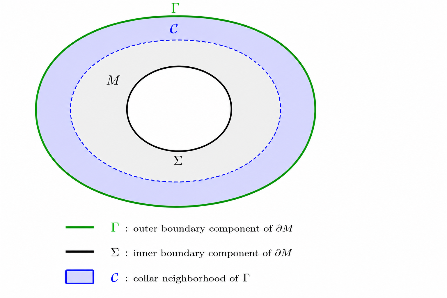
For \(g_\star\in\{g,\widetilde{g}\}\), we denote by \(\Lambda_{g_\star,\Gamma}\) the Dirichlet–to–Neumann map on \(\Gamma\), with zero Dirichlet data prescribed on \(\partial M\setminus\Gamma\).

Our first local-to-global propagation result is the following.

3 Proof of Theorem 2↩︎

We shall use the exponential spectral unique continuation theorem of Jerison–Lebeau [19]. We also refer to the interpolation inequality of Lebeau–Zuazua [20]; see also Lebeau–Robbiano [21] and Le Rousseau–Lebeau [22]. We recall that \[\label{Lap-spectrum} 0=\lambda_0<\lambda_1<\lambda_2<\cdots\tag{15}\] are the distinct eigenvalues of the Laplace–Beltrami operator on \(K\), and \[\label{spectral-proj} P_k:L^2(K)\longrightarrow E_{\lambda_k}\tag{16}\] is the associated spectral projection. Assume that \[g=\widetilde{g} \qquad\text{on }K=\partial M,\] and set \[\label{A-def} A=\Lambda_g-\Lambda_{\widetilde{g}}.\tag{17}\] Since \(\Lambda_{g,\mathcal{O}} = \Lambda_{\widetilde{g},\mathcal{O}},\) we have, for every \(\psi\in C_c^\infty(\mathcal{O}),\) \[\label{Apsi-local} A\psi=0 \qquad\text{on }\mathcal{O}.\tag{18}\] Assume moreover that there exist constants \(C>0\) and \(\varepsilon>0\) such that \[\label{exp-decay} \|P_kA\|_{\mathcal{L}(L^2(K))} \le Ce^{-\varepsilon\sqrt{\lambda_k}}, \qquad k\ge0.\tag{19}\] Then \[\label{exp-decay-Apsi} \|P_k(A\psi)\|_{L^2(K)} \le Ce^{-\varepsilon\sqrt{\lambda_k}} \|\psi\|_{L^2(K)},\tag{20}\] so that the spectral components of \(A\psi\) satisfy a fixed exponential decay. Since \(A\psi=0\) on \(\mathcal{O}\), all the assumptions of Proposition 5.6 in Le Rousseau–Lebeau [22] are fulfilled. Therefore, \[\label{Apsi-zero} A\psi=0 \qquad\text{on }K.\tag{21}\] Now, since \(A\) is self-adjoint, the same argument as in the proof of Theorem 1 yields \[\langle Au,\psi\rangle = \langle u,A\psi\rangle = 0,\] for every \(u\in C^\infty(K)\) and every \(\psi\in C_c^\infty(\mathcal{O})\). Hence \[Au=0 \qquad\text{on }\mathcal{O}.\] Moreover, by 19 , \[\label{exp-decay-Au} \|P_k(Au)\|_{L^2(K)} \le Ce^{-\varepsilon\sqrt{\lambda_k}} \|u\|_{L^2(K)}.\tag{22}\] Proposition 5.6 of [22] applies once again and yields \[\label{Au-zero} Au=0 \qquad\text{on }K.\tag{23}\] Since this holds for every \(u\in C^\infty(K),\) we conclude that \(\Lambda_g=\Lambda_{\widetilde{g}}.\) This completes the proof.

4 The Quasi–Analytic Propagation Principle↩︎

We now recall the quasi–analytic propagation theorem that will replace the exponential spectral unique continuation result used in the proof of Theorem 2. We assume in this section that \(K\) is a compact connected Riemannian symmetric space. This additional structure is required in order to apply the theorem of Ganguly and Thangavelu. Typical examples are \[K=\mathbb{S}^d,\qquad K=\mathbb{T}^d,\qquad K=\mathbb{RP}^d,\] more generally compact rank-one symmetric spaces and finite products of such spaces.

We keep the notation introduced above: \(\lambda_k\) denotes the distinct eigenvalues of the Laplace–Beltrami operator on \(K\), and \(P_k:L^2(K)\to E_{\lambda_k}\) the corresponding spectral projections.

The following result is Theorem 1.4 of Ganguly and Thangavelu [11].

This proposition will be used in exactly the same way as the exponential spectral propagation result in the proof of Theorem 2. Namely, once the local equality of the Dirichlet–to–Neumann maps gives \(A\psi=0\) on \(\mathcal{O}\), Proposition 8 will propagate this vanishing to all of \(K\), provided suitable quasi–analytic estimates on the spectral projections \(P_k(A\psi)\) are available. The next sections are devoted precisely to proving these estimates in the warped product setting.

5 Separable manifolds and diagonalization of the Dirichlet–to–Neumann map↩︎

In this section, we investigate the simple warped product model introduced in Section 1 that will serve as a testing ground for the quasi-analytic propagation mechanism developed in this paper. Besides allowing for an explicit diagonalization of the Dirichlet–to–Neumann map, this framework captures the main ideas of the argument and may provide useful insight toward future extensions to more general geometric settings.

5.1 Geometric framework↩︎

Throughout this section, we consider a class of \(d\)-dimensional manifolds with boundary of the form \[\label{eq:manifold} M=(0,1]\times K,\tag{24}\] where \(d\geq 3\) and where \(K\) is a compact, connected and orientable \((d-1)\)-dimensional Riemannian symmetric space. The manifold \(M\) has a single boundary component, \[\partial M=\{1\}\times K,\] which will be identified with \(K\).

We equip \(M\) with a warped product metric of the form \[\label{Metric} g=c(r)^4\big(dr^2+r^2 g_K\big),\tag{25}\] where \(g_K\) is the canonical metric associated with \(K\), and where \[c:[0,1]\longrightarrow (0,\infty)\] is a positive function of class \(C^m\), with \(m\ge 2\). As explained in Section 1, the geometric setting described above allows for both regular and singular Riemannian structures. For the analysis of the Dirichlet–to–Neumann map, it is convenient to introduce the logarithmic variable \[x=-\log r, \qquad x\in [0,+\infty).\] In these coordinates, the manifold acquires the cylindrical representation \[\label{Metricx} g=f(x)^4\bigl(dx^2+g_K\bigr),\tag{26}\] where \[f(x)=c(e^{-x})\,e^{-x/2}.\] Since \(c\) admits a Taylor expansion of order \(m\) at the origin, one obtains the asymptotic behavior \[\label{f} f(x) = e^{-x/2} +\sum_{k=1}^{m} c_k e^{-(k+\frac{1}{2})x} +o\!\left(e^{-(m+\frac{1}{2})x}\right), \qquad x\to+\infty,\tag{27}\] for suitable real coefficients \(c_k\).

The simplest example in this class is obtained by taking \(K=S^{d-1}\) equipped with its round metric and choosing \(c(r)\equiv 1.\) In that case, \(g\) coincides with the Euclidean metric on the unit ball of \(\mathbb{R}^d\), while \(f(x)=e^{-x/2}.\) More generally, when \(K=S^{d-1}\), the metrics 25 may be viewed as conformal radial deformations of the Euclidean ball, the deformation being entirely encoded by the conformal factor \(c\).

5.2 The Dirichlet–to–Neumann map and the Steklov spectrum↩︎

The main object of interest in this work is the Dirichlet–to–Neumann operator associated with the class of manifolds introduced above.

Given \(\psi\in H^{1/2}(K),\) we consider the boundary value problem \[\label{Dirichlet} \left\{ \begin{align} -\Delta_g u &=0 \qquad &&\text{on } M,\\ u&=\psi &&\text{on } \partial M. \end{align} \right.\tag{28}\]

The Dirichlet–to–Neumann map is first defined in the weak sense by the Green identity \[\langle \Lambda_g\psi,\varphi\rangle = \int_M \langle du,dv\rangle_g\, dV_g,\] for every \(\varphi\in H^{1/2}(K)\) and every function \(v\in H^1(M)\) satisfying \[v|_{\partial M}=\varphi,\] where \(u\) is the unique solution of 28 with boundary value \(\psi\). When the metric, the boundary data, and the solution are sufficiently regular, this weak definition agrees with the classical expression \[\label{DN} \Lambda_g\psi = \partial_\nu u\big|_{\partial M},\tag{29}\] where \(\nu\) denotes the outward unit normal vector field along \(\partial M\). Indeed, in the regular case, the endpoint \(r=0\) corresponds to a single point \(p\) in the smooth compact completion \(\check M\), so that \(M=\check M\setminus\{p\}.\) Since \(\dim\check M\ge3\), the point \(\{p\}\) has zero \(H^1\)-capacity. Hence \[H^1(\check M)=H^1_0(\check M\setminus\{p\}),\] where \(H^1_0(\check M\setminus\{p\})\) denotes the closure of \(C_c^\infty(\check M\setminus\{p\})\) in the \(H^1\)-norm. Therefore, the integration by parts formula on \(M\) follows by density from the same formula for compactly supported smooth functions on \(\check M\setminus\{p\}\). In particular, the removed point \(p\) produces no additional boundary contribution.

The operator \(\Lambda_g\) is self-adjoint on \(L^2(\partial M,dS_g)\) and has compact resolvent. Its spectrum, referred to as the Steklov spectrum of \((M,g)\), therefore consists of a discrete sequence of real eigenvalues, counted with multiplicities, \[\label{eq:Steklov-spectrum} 0=\sigma_0\le \sigma_1\le \sigma_2\le \cdots, \qquad \sigma_j\to+\infty.\tag{30}\] We denote by \[\label{eq:Steklov-distinct} 0=\tau_0<\tau_1<\tau_2<\cdots\tag{31}\] the distinct Steklov eigenvalues, that is, the spectrum of \(\Lambda_g\) without multiplicities. We refer to [23] for a general introduction to Steklov spectral theory.

5.3 Separation of variables↩︎

We first rewrite the harmonic equation 28 in the cylindrical variable \[x=-\log r\in[0,+\infty).\] Introducing \[v=f^{d-2}u,\] a direct computation shows that the equation \(-\Delta_g u=0\) becomes \[\label{LaplaceEq} \Bigl(-\partial_x^2-\Delta_{g_K}+q_f(x)\Bigr)v = -\frac{(d-2)^2}{4}\,v,\tag{32}\] where the effective potential \(q_f\) is defined by \[\label{qf} q_f(x) = \frac{(f^{d-2})''(x)}{f^{d-2}(x)} -\frac{(d-2)^2}{4}.\tag{33}\] In terms of the original radial variable \(r=e^{-x}\), the potential can be written as \[\label{potradial} q_f(x) = (d-2)\left( (d-3)r^2 \left(\frac{c'(r)}{c(r)}\right)^2 + r^2\frac{c''(r)}{c(r)} + (d-1)r\frac{c'(r)}{c(r)} \right).\tag{34}\] Moreover, the asymptotic expansion 27 implies \[\label{Asympqf} q_f(x)=O(e^{-x}), \qquad x\to+\infty.\tag{35}\]

The product structure of \((M,g)\) allows us to separate variables. Let \[\label{eq:laplace-spectrum-multiplicity} -\Delta_{g_K}Y_j=\mu_jY_j, \qquad j\ge0,\tag{36}\] where \(\{Y_j\}_{j\ge0}\) is an orthonormal basis of eigenfunctions of \(L^2(K,dV_{g_K})\). Recall that the distinct eigenvalues of \(-\Delta_{g_K}\) are denoted by \[\label{eq:laplace-spectrum-distinct} 0=\lambda_0<\lambda_1<\lambda_2<\cdots,\tag{37}\] while \[\label{eq:laplace-spectrum-full} 0=\mu_0\le \mu_1\le \mu_2\le\cdots\tag{38}\] denotes the spectrum counted with multiplicities. Expanding \[\label{SepaV} v(x,\omega) = \sum_{j\ge0}v_j(x)Y_j(\omega),\tag{39}\] equation 32 reduces to the family of one-dimensional equations \[\label{ODE-x} -v_j''+q_f(x)v_j = -\kappa_j^2v_j, \qquad x\in(0,+\infty),\tag{40}\] where \[\label{eq:kappa-j} \kappa_j = \sqrt{\mu_j+\frac{(d-2)^2}{4}}.\tag{41}\] This naturally leads to the Schrödinger operator \[\label{Hoperator} H = -\frac{d^2}{dx^2}+q_f(x)\tag{42}\] acting on the half-line, and to the associated spectral equation \[\label{SLz} -v''+q_f(x)v=zv, \qquad z\in\mathbb{C}.\tag{43}\]

Let \(\{C_0(\cdot,z),S_0(\cdot,z)\}\) be the fundamental system of solutions of 43 normalized by \[\label{FSS} C_0(0,z)=1, \qquad C_0'(0,z)=0, \qquad S_0(0,z)=0, \qquad S_0'(0,z)=1.\tag{44}\] Their Wronskian is therefore given by \[\label{Wronskian} W(C_0,S_0)=1.\tag{45}\] Since \(q_f\in L^1(0,+\infty)\) by 35 , the operator \(H\) is in the limit-point case at infinity. Consequently, for every \(z\in\mathbb{C},\) there exists, up to a multiplicative constant, a unique solution \(S_\infty(\cdot,z)\) of 43 belonging to \(L^2\) in a neighborhood of \(+\infty\), (see [24], Theorem XI.57 where our spectral parameter \(z= k^2\)). Writing \[\label{WeylSolution} S_\infty(x,z) = A(z)\bigl(C_0(x,z)+M(z)S_0(x,z)\bigr),\tag{46}\] defines the Weyl–Titchmarsh function \(M(z)\). Using 45 , we obtain

\[\label{WT} M(z) = \frac{S_\infty'(0,z)}{S_\infty(0,z)}.\tag{47}\]

Finally, the Dirichlet–to–Neumann map is diagonal with respect to the Hilbert basis of harmonics \(\{Y_j\}_{j\ge0}\). Thus, if \(\psi=\sum_{j\ge0}\psi_jY_j,\) then \[\label{GlobalDN} \Lambda_g\psi = \sum_{j\ge0} (\Lambda_g^{(j)}\psi_j)\,Y_j,\tag{48}\] where \(\Lambda_g^{(j)}\) is the scalar by which \(\Lambda_g\) acts on \(\mathrm{span}\{Y_j\}\). The computation is identical to the one carried out in [14]. If \(\mu_j=\lambda_k,\) with \(\mu_j\) counted with multiplicities and \(\lambda_k\) denoting a distinct eigenvalue, then \[\label{DNk} \Lambda_g^{(j)} = \frac{(d-2)f'(0)}{f^3(0)} - \frac{M(-\rho_k^2)}{f^2(0)},\tag{49}\] where \[\label{eq:rho-k} \rho_k = \sqrt{\lambda_k+\frac{(d-2)^2}{4}}, \qquad k\ge0.\tag{50}\]

Since the coefficient in 49 depends only on the corresponding distinct eigenvalue \(\lambda_k\), the operator \(\Lambda_g\) acts by scalar multiplication on each eigenspace \[\label{eq:eigenspace-k} E_{\lambda_k} = \ker(-\Delta_{g_K}-\lambda_k).\tag{51}\] Hence \[\label{DN-projection} \Lambda_g = \sum_{k\ge0} \left( \frac{(d-2)f'(0)}{f^3(0)} - \frac{M(-\rho_k^2)}{f^2(0)} \right) P_k.\tag{52}\] Since the Weyl–Titchmarsh function \(M\) is strictly increasing, (see Lemma 2.3 in [14]), the distinct Steklov eigenvalues are given by \[\label{LinkSteklovWT1} \tau_k = \frac{(d-2)f'(0)}{f^3(0)} - \frac{M(-\rho_k^2)}{f^2(0)}, \qquad k\ge0.\tag{53}\]

5.4 A weighted Laplace estimate↩︎

The purpose of this subsection is to construct a weight function whose Laplace transform decays almost exponentially. This elementary estimate will play a key role in the proof of the quasi-analytic propagation result.

Let \(\theta:[T,\infty)\longrightarrow(0,\infty)\) be a decreasing function such that \(\lim_{t\to\infty}\theta(t)=0.\) We define \[\label{Phi-I-def} \Phi(x) = \inf_{t\ge T} \bigl(2xt-t\theta(t)\bigr), \qquad x>0,\tag{54}\] and \[I(\rho) = \int_0^\varepsilon e^{-2\rho x}e^{\Phi(x)}\,dx,\] where \(\varepsilon>0\) is as in Theorem 5. We have the following result.

5.5 A Weyl–Titchmarsh estimate↩︎

We now recall several estimates proved in [14] that will be used in the proof of our quasi-analytic propagation result. The key point is that the difference of the Weyl–Titchmarsh functions can be represented as a Laplace transform involving the difference of the effective potentials \(q_{\widetilde{f}}\) and \(q_f\).

According to Lemma 4.4 of [14] (with \(p=1\)), there exists a kernel \[K_1:\{(x,t)\,;\,0\le t\le x\}\longrightarrow \mathbb{R}\] such that, for every \(0<\alpha<1\), there exists a constant \(C_{\alpha}>0\) satisfying \[\label{K1-estimate} \left| \partial_x^k\partial_t^\ell K_1(x,t) \right| \le C_{\alpha}\,e^{-\alpha x}, \qquad 0\le t\le x, \qquad k,\ell\le m-1.\tag{55}\] We then define the Volterra operator \(B\) by \[\label{Volterra-operator} h\mapsto Bh(x) = h(x) + \int_0^x K_1(x,t)h(t)\,dt.\tag{56}\] Lemma 4.5 of [14] asserts that, for all sufficiently large \(\rho\), \[\label{WT-B} S_\infty(0,-\rho^2)\widetilde{S}_\infty(0,-\rho^2) \bigl( M(-\rho^2)-\widetilde{M}(-\rho^2) \bigr) = \int_0^\infty e^{-2\rho x} B[q_{\widetilde{f}}-q_f](x)\,dx .\tag{57}\] Moreover, Corollary 4.3 of [14] yields \[\label{WT-origin} S_\infty(0,-\rho^2) = 1+O(\rho^{-1}), \qquad \widetilde{S}_\infty(0,-\rho^2) = 1+O(\rho^{-1}), \qquad \rho\to+\infty .\tag{58}\] Combining 57 and 58 , we obtain the existence of positive constants \(C\) and \(\rho_0\) such that \[\label{WT-B-estimate} \left| M(-\rho^2)-\widetilde{M}(-\rho^2) \right| \le C \left| \int_0^\infty e^{-2\rho x} B[q_{\widetilde{f}}-q_f](x)\,dx \right|,for\rho\ge \rho_0\,.\tag{59}\]

We now estimate the right-hand side of 59 . We first deal with the contribution of the interval \((1,\infty)\). Recall that \[\label{AsympQf} q_f(x)=O(e^{-x}), \qquad x\to+\infty .\tag{60}\] Since \(q_f\) and \(q_{\widetilde{f}}\) belong to \(C^{m-2}([0,\infty))\) and satisfy 60 , we have \[\label{Hdelta} q_{\widetilde{f}}-q_f\in H_\delta, \qquad 0<\delta<2, \qquad H_\delta = \Bigl\{ q\,;\, \int_0^\infty |q(x)|^2e^{\delta x}\,dx<\infty \Bigr\}.\tag{61}\] Moreover, by Proposition 4.6 of [14], for every \(0<\delta<1\), the Volterra operator \(B\) is an isomorphism \(B:H_\delta\longrightarrow H_\delta.\) Consequently, for \(0<\delta <1\), \(B[q_{\widetilde{f}}-q_f]\in H_\delta .\) Therefore, by the Cauchy–Schwarz inequality, \[\label{tail-cs} \left| \int_\varepsilon^\infty e^{-2\rho x} B[q_{\widetilde{f}}-q_f](x)\,dx \right| \le \left( \int_\varepsilon^\infty e^{-(4\rho+\delta)x}\,dx \right)^{1/2} \left\| B[q_{\widetilde{f}}-q_f] \right\|_{H_\delta}.\tag{62}\] Thus, \[\label{tail-estimate} \left| \int_\varepsilon^\infty e^{-2\rho x} B[q_{\widetilde{f}}-q_f](x)\,dx \right| \le C e^{-2\rho\varepsilon}, \qquad \rho>0 .\tag{63}\]

We now estimate the contribution of the interval \((0,\varepsilon)\) in the right-hand side of 59 . To this end, we assume that \[\label{quasi-analytic-closeness-f} \left| \partial_x^j(f-\widetilde{f})(x) \right| \le C e^{\Phi(x)}, \qquad 0<x<\varepsilon, \qquad j=0,1,2.\tag{64}\] Consequently, since \(q_f\) depends smoothly on \(f\), \(f'\), and \(f''\), and since \(f\) and \(\widetilde{f}\) are bounded away from zero, there exists \(C>0\) such that \[\label{quasi-analytic-closeness-q} |q_{\widetilde{f}}(x)-q_f(x)| \le C e^{\Phi(x)}, \qquad 0<x<1.\tag{65}\] Moreover, by 55 , the kernel \(K_1\) is bounded on \(\{0\le t\le x\le\varepsilon\}\). Hence, using 56 , \[|B[q_{\widetilde{f}}-q_f](x)| \le |q_{\widetilde{f}}(x)-q_f(x)| + C\int_0^x |q_{\widetilde{f}}(t)-q_f(t)|\,dt.\] Since \(\Phi\) is increasing, 65 yields \[|q_{\widetilde{f}}(t)-q_f(t)| \le C e^{\Phi(x)}, \qquad 0<t<x,\] and therefore \[\label{Bq-local-bound} |B[q_{\widetilde{f}}-q_f](x)| \le C e^{\Phi(x)}, \qquad 0<x<\varepsilon.\tag{66}\] It follows that \[\left| \int_0^\varepsilon e^{-2\rho x} B[q_{\widetilde{f}}-q_f](x)\,dx \right| \le C \int_0^\varepsilon e^{-2\rho x}e^{\Phi(x)}\,dx.\] Using Lemma 1, we obtain \[\label{local-laplace-estimate} \left| \int_0^\varepsilon e^{-2\rho x} B[q_{\widetilde{f}}-q_f](x)\,dx \right| \le C e^{-\rho\,\theta(\rho)}, \qquad \rho\ge T.\tag{67}\] Combining 59 , 63 and 67 , we obtain \[\left| M(-\rho^2)-\widetilde{M}(-\rho^2) \right| \le C\bigl(e^{-\rho\,\theta(\rho)}+e^{-2\rho\varepsilon}\bigr).\] Since \(\theta(\rho)\to0\) as \(\rho\to+\infty\), it follows that \(e^{-2\rho\varepsilon}=O(e^{-\rho\,\theta(\rho)})\). Hence there exist positive constants \(C\) and \(\rho_0\) such that \[\label{WT-final-decay} \left| M(-\rho^2)-\widetilde{M}(-\rho^2) \right| \le C e^{-\rho\,\theta(\rho)},for\rho\geq \rho_0\,.\tag{68}\]

5.6 A pointwise estimate for spectral projectors↩︎

Let \(K\) be a compact symmetric space endowed with its Riemannian metric \(g_K\). Let \[-\Delta_{g_K}Y_{k,\alpha} = \lambda_k Y_{k,\alpha}, \qquad \alpha=1,\dots,d_k,\] where \(\{Y_{k,\alpha}\}_{\alpha=1}^{d_k}\) is an orthonormal basis of the eigenspace \[E_k=\ker(-\Delta_{g_K}-\lambda_k), \qquad d_k=\dim E_k .\] For \(\psi\in L^2(K)\), the orthogonal projection onto \(E_k\) is given by \[\label{eq:PkPsi-expansion} P_k\psi = \sum_{\alpha=1}^{d_k} \langle \psi,Y_{k,\alpha}\rangle_{L^2(K)} \,Y_{k,\alpha}.\tag{69}\] Applying the Cauchy–Schwarz inequality, we obtain \[\label{eq:PkPsi-CS} |P_k\psi(\omega)| \le \|P_k\psi\|_{L^2(K)} \left( \sum_{\alpha=1}^{d_k} |Y_{k,\alpha}(\omega)|^2 \right)^{1/2}, \qquad \omega\in K.\tag{70}\] Since \(K\) is a compact symmetric space, the function \[\label{eq:Zk-definition} Z_k(\omega) = \sum_{\alpha=1}^{d_k} |Y_{k,\alpha}(\omega)|^2.\tag{71}\] is invariant under the transitive action of the isometry group of \(K\), (see, for instance, Helgason [25]). Hence \(Z_k\) is constant on \(K\). Integrating over \(K\), we obtain \[\label{eq:Zk-constant} Z_k(\omega)\,\mathop{\mathrm{Vol}}(K) = \sum_{\alpha=1}^{d_k} \int_K |Y_{k,\alpha}|^2\,dV_{g_K} = d_k.\tag{72}\] and therefore \[\label{eq:addition-formula} \sum_{\alpha=1}^{d_k} |Y_{k,\alpha}(\omega)|^2 = \frac{d_k}{\mathop{\mathrm{Vol}}(K)}, \qquad \omega\in K.\tag{73}\] We conclude that \[\label{eq:PkPsi-pointwise-L2} |P_k\psi(\omega)| \le \sqrt{\frac{d_k}{\mathop{\mathrm{Vol}}(K)}} \,\|P_k\psi\|_{L^2(K)} \le \sqrt{\frac{d_k}{\mathop{\mathrm{Vol}}(K)}} \,\|\psi\|_{L^2(K)}.\tag{74}\] This estimate will be used repeatedly in the sequel.

6 Proof of Theorem 5↩︎

We now conclude the proof of the local-to-global propagation result. The only new ingredient is the quasi–analytic propagation theorem of Ganguly and Thangavelu, which replaces the exponential spectral propagation result used in the proof of Theorem 2. We begin by an elementary lemma:

Now, assume that \[\label{quasi-analytic-final} \left| \partial_x^j(f-\widetilde{f})(x) \right| \le C e^{\Phi(x)}, \qquad 0<x<\varepsilon, \qquad j=0,1,2.\tag{75}\] By the previous lemma, \[e^{\Phi(x)}\longrightarrow0 \qquad\text{as }x\to0^+.\] Hence 75 implies \[\label{boundary-jets-final} f^{(j)}(0)=\widetilde{f}^{(j)}(0), \qquad j=0,1,2.\tag{76}\] Let \[\label{eq:F-definition} F=(\Lambda_g-\Lambda_{\widetilde{g}})\psi, \qquad \psi\in C_c^\infty(\mathcal{O}).\tag{77}\] If the local Dirichlet–to–Neumann maps coincide on \(\mathcal{O}\), we have \(F=0\) on \(\mathcal{O}\). Combining the diagonalization formula for the Dirichlet–to–Neumann map with the boundary identities 76 , we obtain \[\label{eq:PkF-WT} P_kF = -\frac{1}{f^2(0)} \Bigl( M(-\rho_k^2)-\widetilde{M}(-\rho_k^2) \Bigr) P_k\psi.\tag{78}\] where \[\label{eq:rho-k-definition} \rho_k = \sqrt{\lambda_k+\frac{(d-2)^2}{4}}.\tag{79}\] Using 68 , we obtain the pointwise estimate \[\label{eq:PkF-pointwise} |P_kF(\omega)| \le C\, e^{-\rho_k\theta(\rho_k)} |P_k\psi(\omega)|, \qquad k \geq 0.\tag{80}\] On the other hand, it follows from 74 that \[\label{eq:PkPsi-pointwise-bound} |P_k\psi(\omega)| \le C\, d_k^{1/2}\, \|\psi\|_{L^2(K)}, \qquad \omega\in K.\tag{81}\] By the local Weyl law (see, e.g., [26]), \[\label{eq:multiplicity-bound} d_k \le C(1+\lambda_k)^{\frac{\dim K-1}{2}}.\tag{82}\] Combining 80 , 81 and 82 , we obtain \[\label{eq:PkF-final} |P_kF(\omega)| \le C (1+\lambda_k)^{\frac{\dim K-1}{4}} e^{-\rho_k\theta(\rho_k)}, \qquad \omega\in K.\tag{83}\] Since \(\rho_k\sim\sqrt{\lambda_k}\), possibly replacing \(\theta\) by a smaller function with the same properties, we obtain \[\label{GT-estimate} |P_kF(\omega)| \le C e^{-\sqrt{\lambda_k}\,\theta(\sqrt{\lambda_k})}, \qquad \omega\in K.\tag{84}\]

Therefore \(F\) satisfies the assumptions of Proposition 8. Hence \(F \equiv 0\) on \(K\). The remainder of the proof is identical to that of Theorem 2. Since \(f(0)=\widetilde{f}(0)\), the operator \(A=\Lambda_g-\Lambda_{\widetilde{g}}\) is self-adjoint on \(L^2(K,dS_K)\). Arguing exactly as in the proof of Theorem 2, we conclude that \(Au=0\) on \(K\) for every \(u\in C^\infty(K)\). Therefore, \(\Lambda_g=\Lambda_{\widetilde{g}},\) which completes the proof.

Acknowledgements↩︎

This work has received funding from the European Research Council (ERC) under the European Union’s Horizon 2020 research and innovation programme through the grant agreement 862342 (A.E.). A.E. is partially supported by the grants CEX2023-001347-S, RED2022-134301-T, and PID2022-136795NB-I00 funded by the Spanish Ministry of Science and Innovation. F.N. thanks the French GDR Dynqua for his support. N.K. is supported by NSERC grant RGPIN 105490-2025.

References↩︎