Bayesian Best-Arm Identification with Abstention: A Polynomial-to-Exponential Phase Transition
January 01, 1970
Abstract
We study the Bayesian fixed-budget best-arm identification problem in which a learner can abstain from making a terminal recommendation. Subject to an abstention budget \(\alpha\), we analyze the probability of undetected error–the risk of recommending a suboptimal arm without abstaining. Our central finding is that abstention induces a phase transition: without abstention, the error probability decays polynomially in the sampling budget \(T\); in contrast, introducing any small positive abstention budget shifts this to an exponential decay. For Gaussian priors and rewards, in the regime \(T\to\infty\) followed by \(\alpha\downarrow0\), we establish exact matching information-theoretic lower bounds and algorithmic upper bounds on the optimal error exponent, which takes the form \(\exp(-\frac{\alpha^{2}T}{8\kappa_{\nu}^{2}})\). The hardness parameter \(\kappa_{\nu}\) represents the prior density of the top-two gap at zero, highlighting that nearly tied instances drive the fundamental error. We introduce an adaptive algorithm, PGWS, that successfully achieves this optimal exponent by expending its abstention budget on statistically ambiguous instances. We further demonstrate that this polynomial-to-exponential improvement is exclusively a Bayesian phenomenon–in the frequentist setting, abstention only affects lower-order exponent terms. We also extend our results beyond the Gaussian model.
1 Introduction↩︎
1.1 Problem Overview and Motivation↩︎
Fixed-Budget Best-Arm Identification (FB-BAI) [1]–[3] is a canonical pure exploration problem in sequential decision making. A learner is given a sampling budget, adaptively collects noisy observations from a set of \(K\) arms with unknown mean rewards, and finally recommends the arm believed to have the largest mean. This formulation captures the statistical core of ranking and selection, online experimentation, and treatment-selection problems, where samples are costly and the objective is to make a reliable terminal recommendation rather than to maximize reward during the experiment [1], [4], [5].
Typical FB-BAI formulations require a firm terminal recommendation after the sampling budget is exhausted. In many applications, however, this forced decision, in which the decision maker commits to one of the \(K\) arms, may pose undue risks. When the collected evidence is ambiguous, the decision maker may defer the decision, run a follow-up experiment, escalate the case to an expert, or choose a conservative default action. This motivates a FB-BAI model with terminal abstention option: after sampling, the learner may either recommend an arm or output an inconclusive decision.
Abstention changes the notion of error. A policy that always abstains never makes an incorrect recommendation, but it is not useful. We therefore treat abstention as a scarce resource: the learner must keep the probability of abstention below a prescribed level \(\alpha\). Subject to this constraint, the performance criterion is the probability of an undetected error, namely the probability that the learner does not abstain but recommends a suboptimal arm. Informally, let \(a^\star\) denote the best arm, \(?\) be the abstention decision, and \(\hat{a}\in [K]\cup\{?\}\) be the terminal output. The objective is to minimize \[\mathbb{P}\big(\hat{a}\notin\{a^\star,?\}\big), \quad \textrm{subject to} \quad \mathbb{P}(\hat{a}=?)\le \alpha .\]
This paper studies the problem in a Bayesian fixed-budget setting, where the unknown reward means are drawn from known priors. The Bayesian formulation is natural when the same experimental protocol is repeatedly applied to related instances, or when historical data provide a prior model for plausible reward configurations. It is also the setting in which the effect of abstention is particularly pronounced. Under a continuous prior, the Bayes error probability of forced-decision (i.e., without abstention) FB-BAI is dominated by instances in which the two best arms are nearly tied. These instances are rare, but they are also the hardest to resolve with a finite sampling budget.
The central observation of this paper is that a small abstention budget allows the learner to spend its inconclusive decisions precisely on these statistically ambiguous near-tie cases. We show that this fundamentally results in a phase transition of the behavior of Bayesian BAI: even a small positive abstention budget substantially reduces the forced-decision polynomially small Bayes error probability into an exponentially small Bayes undetected error probability. We derive this exponent and show that it is governed by the amount of prior probability near top-two ties. The rest of the paper formalizes this principle, develops an adaptive algorithm that attains the optimal exponent, and contrasts the Bayesian phenomenon with the frequentist setting.
1.2 Problem Formulation and Top-Two Gap Complexity↩︎
We now introduce the formal model. For an integer \(K\ge 2\), let \([K]:=\{1,\ldots,K\}\). The learner is given a fixed sampling budget \(T\) and a collection of \(K\) arms. Arm \(i\in[K]\) has an unknown mean reward \(\mu_i\). We study a Bayesian model in which the mean vector \(\mu=(\mu_1,\ldots,\mu_K)\) is drawn from a known product Gaussian prior \[P_\nu(\mathrm{d}\mu) := \bigotimes_{i=1}^K \mathcal{N}(\nu_i,\sigma_0^2)(\mathrm{d}\mu_i),\] where the prior means \(\nu_1,\ldots,\nu_K\in\mathbb{R}\) and prior variance (which is common to all arms) \(\sigma_0^2>0\) are fixed and known. We define the best arm \(a^\star=a^\star(\mu):=\argmax_{i\in[K]}\mu_i\) which is unique almost surely since the prior \(P_\nu\) is continuous. Conditional on \(\mu\), the rewards from the arms are independent (across arms and time) and normally distributed: \[Y_{i,s}\mid \mu_i \sim \mathcal{N}(\mu_i,1), \qquad s \in \mathbb{N},~i \in [K].\]
1.2.0.1 Policies and Probability Laws.
A policy \(\pi\) consists of a sequence of sampling rules and a terminal decision rule. At each round \(t=1,\ldots, T\), the policy selects an arm \(A_t \in [K]\). Conditional on \(A_t=i\) and the mean vector \(\mu\), the learner observes a random sample \(X_t=Y_{i, N_i(t)}\) where \(N_i(t):=\sum_{s=1}^t \mathbb{1}\{A_s=i\}\) denotes the number of samples collected from arm \(i\) up to and including time \(t\). The choice of the arm to be pulled \(A_t\) depends on the previous arm choices \(\{A_s\}_{s=1}^{t-1}\) and observations \(\{ X_s \}_{s=1}^{t-1}\). At the terminal time \(T\), the policy recommends an arm from \([K]\) as the estimated best arm or an abstention decision denoted as \(?\). The class of all such policies is denoted as \(\Pi_T\).
For a fixed mean vector \(\mu\), we write \(\mathbb{P}_\mu^\pi\) and \(\mathbb{E}_\mu^\pi\) for the probability and expectation over the reward realizations and the potential randomization of the policy. The joint Bayesian law is the mixture \[\mathbb{P}_\nu^\pi(\cdot) := \int_{\mathbb{R}^K} \mathbb{P}_\mu^\pi(\cdot)\,P_\nu(\mathrm{d}\mu),\] and \(\mathbb{E}_\nu^\pi\) is defined analogously. When the policy (resp. probability law) is clear from context, we suppress the superscript \(\pi\) (resp. subscript \(\nu\)).
1.2.0.2 Terminal Decisions with Abstention.
At the end of the experiment, the learner outputs \(\hat{a}_T\in[K]\cup\{?\}\), where \(?\) denotes abstention, an inconclusive decision. The learner makes an undetected error if it recommends an arm and the recommended arm is not the true best arm, i.e., the event \(\big\{\hat{a}_T\notin\{a^\star,?\} \big\} = \big\{\hat{a}_T\in[K],\;\hat{a}_T\neq a^\star\big\}\) occurs.
For a policy \(\pi\in\Pi_T\), define its Bayes abstention probability and Bayes undetected error probability respectively as \[\mathcal{A}_T(\pi) := \mathbb{P}_\nu^\pi(\hat{a}_T=?) \quadand\quad \mathcal{E}_T(\pi) := \mathbb{P}_\nu^\pi \bigl(\hat{a}_T\in[K],\;\hat{a}_T\neq a^\star(\mu)\bigr).\] Given an abstention budget \(\alpha\in(0,1)\), let \[\Pi_T(\alpha) := \{\pi\in\Pi_T:\mathcal{A}_T(\pi)\le\alpha\}.\] The optimal Bayes undetected error probability is \[\label{eq:bayes-risk-abstention} \mathfrak E_{T}(\alpha) := \inf_{\pi\in\Pi_T(\alpha)} \mathcal{E}_T(\pi).\tag{1}\] For later comparison, we also define the optimal forced-decision Bayes probability of misidentification (in which abstention is not allowed) as \[\mathfrak E_{T}(0) := \inf_{\pi\in\Pi_T:\,\hat{a}_T\in[K]\;{\rm a.s.}} \mathbb{P}_\nu^\pi(\hat{a}_T\neq a^\star)= \inf_{\pi\in\Pi_T(0) } \mathbb{P}_\nu^\pi(\hat{a}_T\neq a^\star)\;. \label{eqn:CT0}\tag{2}\]
1.2.0.3 Top-Two Gap Complexity.
We define the top-two gap \[\Gamma:=\mu_{(1)}-\mu_{(2)},\] where \(\mu_{(1)}>\mu_{(2)}>\cdots>\mu_{(K)}\) denote the means of the arms arranged in decreasing order. Theorems 1 and 2 identify the density of \(\Gamma\) at zero as the fundamental hardness parameter for the Bayesian BAI problem with abstention.
For each arm \(i\), we denote the prior density and distribution function of \(\mu_i\) as \[f_i(x) := \frac{1}{\sigma_0} \phi\left(\frac{x-\nu_i}{\sigma_0}\right), \quadand\quad F_i(x) := \Phi\left(\frac{x-\nu_i}{\sigma_0}\right),\] where \(\phi(x)=\frac{1}{\sqrt{2\pi}}e^{-x^2/2}\) and \(\Phi(x)=\int_{-\infty}^x \phi(u)\, \mathrm{d}u\) are the standard normal density and cumulative distribution function, respectively.
For a pair of distinct arms \((i,j) \in[K]^2\), define their average midpoint variable as \(X_{ij} \sim \mathcal{N}\!\left( \frac{\nu_i+\nu_j}{2}, \frac{\sigma_0^2}{2} \right)\), and define the top-relevance weight \(w_{ij} := \mathbb{E}\!\left[ \prod_{k\neq i,j} \Phi\!\left(\frac{X_{ij}-\nu_k}{\sigma_0}\right) \right]\). The quantity \(w_{ij}\) is the prior probability, averaged over a local tie value of arms \(i\) and \(j\), that this tied value lies above all remaining arms. Define the hardness parameter for Bayesian BAI with abstention problem as \[\kappa_\nu = \sum_{i\neq j} \int_{\mathbb{R}} f_i(x)f_j(x) \prod_{k\neq i,j}F_k(x)\,\mathrm{d}x = \frac{1}{\sigma_0\sqrt\pi} \sum_{1\le i<j\le K} w_{ij} \exp\!\left( -\frac{(\nu_i-\nu_j)^2}{4\sigma_0^2} \right).\] In Lemma 3, we show that the top-two gap \(\Gamma\) is related to the hardness parameter \(\kappa_\nu\) as follows: \[\mathbb{P}_\nu(\Gamma\le \varepsilon) = \kappa_\nu\varepsilon + o(\varepsilon)\quad as\quad \varepsilon\downarrow 0. \label{eqn:kappa95nu}\tag{3}\] In view of 3 , we see that \(\kappa_\nu\) measures the amount of prior probability assigned to locally ambiguous instances. Specifically, pairs with similar prior means and a realistic chance of being the top two arms contribute more to \(\kappa_\nu\), whereas pairs that are unlikely to be optimal contribute little.
1.3 Main Contributions and Results↩︎
We formulate the fixed-budget BAI with abstention problem under the Bayesian setting. We study this problem under the large-budget and small-abstention probability regime through the iterated limit \(T\to\infty\) followed by \(\alpha\downarrow0\) .
Our main result is a sharp characterization of the exponential rate of decay of the optimal Bayes undetected error probability under abstention. In the Gaussian prior and Gaussian reward model, we prove the information-theoretic lower bound \[\liminf_{\alpha\downarrow0} \liminf_{T\to\infty} \frac{1}{\alpha^2T} \log \mathfrak E_{T}(\alpha) \ge - \frac{1}{8\kappa_\nu^2}.\]
We also propose an adaptive algorithm, Posterior Gap Weighted Sampling with Abstention (PGWS(\(\alpha\))), whose abstention probability is calibrated exactly to \(\alpha\) and whose undetected error probability \(\mathcal{E}_T({\textrm{\mathrm{\small PGWS}}}(\alpha))\) satisfies \[\limsup_{\alpha\downarrow0} \limsup_{T\to\infty} \frac{1}{\alpha^2T} \log \mathcal{E}_T({\textrm{\mathrm{\small PGWS}}}(\alpha)) \le - \frac{1}{8\kappa_\nu^2}.\] Combining these results, we see that the fundamental hardness of the Bayesian BAI with abstention problem depends on the prior through \(\kappa_\nu\), the density of top-two gap at zero. In other words, the complexity is intimately related to the prior probability of instances in which the means of two best arms are nearly the same.
Subsequently, we compare the abstention problem with ordinary (forced-decision) Bayesian BAI, where the learner is compelled to recommend an arm. We establish that the optimal forced-decision Bayes probability of misidentification satisfies \[\liminf_{T\to\infty} \sqrt T\,\mathfrak E_T(0) \ge \sqrt{\frac{2}{\pi}}\,\kappa_\nu .\] Therefore, allowing an \(\alpha\) fraction of abstentions transits the Bayes probability of error from being on the polynomial scale to the exponential scale.
We further demonstrate that this phase transition is inherently Bayesian. In contrast, for any fixed frequentist instance with a positive gap, the error probability of conventional forced-decision FB-BAI already exhibits exponential decay in \(T\); see, e.g., [2]. As a result, terminal abstention cannot improve the leading error exponent and affects only lower-order terms.
Finally, the analysis is extended beyond the Gaussian model. For regular one-parameter reward models, the same exponent takes the form \(1/(8\kappa^2)\), where \(\kappa\) is the top-two gap density evaluated in Fisher–Rao information coordinates; see Eqn. 10 .
We also provide numerical experiments illustrating the benefit of abstention and the practical advantage of our adaptive algorithm which we call PGWS.
1.4 Related work↩︎
1.4.0.1 Best-arm Identification and Ranking and Selection.
Best-arm identification is a central pure-exploration problem in multi-armed bandits. In the fixed-confidence setting, the objective is to identify the best arm with prescribed confidence using as few samples as possible [4], [6], [7]. In the fixed-budget setting, which is our focus, the learner is given a sampling budget and aims to minimize the probability of an incorrect terminal recommendation [1]–[3], [8], [9]. For a fixed instance with a positive gap, this probability typically decays exponentially in the budget, with the exponent determined by instance-dependent complexity. Our work instead studies a Bayesian average over instances and allows terminal abstention. The problem is also related to ranking and selection and ordinal optimization, where the objective is often to maximize the probability of correct selection under a simulation budget [10]–[12]. In contrast to most of that literature, our performance criterion is an abstention-constrained Bayes undetected error probability.
1.4.0.2 Bayesian Best Arm Identification.
Bayesian BAI involves a prior distribution over the unknown reward means. Bayesian algorithms such as Thompson sampling and top-two Thompson sampling have been studied for posterior convergence and BAI [5], [13]. Recent work develops prior-sensitive guarantees for Bayesian BAI: [14] study Gaussian fixed-budget Bayesian BAI, while [15] characterize Bayesian simple-regret rates under continuity assumptions and identify near-tie instances as the leading source of error. Related work also studies prior-dependent allocations in structured Bayesian fixed-budget BAI [16] and fixed-confidence BAI in the Bayesian setting [17]. Our contribution is to add a terminal abstention option and provide a full characterization of the undetected error exponent under an abstention budget.
1.4.0.3 Abstention and Reject-Option Decisions.
Abstention has a long history in statistical decision theory and classification. Classical reject-option rules trade prediction error against rejection [18], and selective prediction studies risk-coverage tradeoffs in supervised learning [19], [20]. These settings are typically passive, whereas our learner actively allocates a fixed sampling budget before deciding whether to recommend or abstain. Bandit models with abstention-like actions include selective sampling for online BAI [21] and regret minimization with per-round abstention [22]. In contrast, our model permits abstention only at the terminal recommendation stage.
1.4.0.4 Erasure Decoding and Undetected Error.
An essential motivation for considering this setup arises from erasure decoding in information theory. In channel coding with an erasure option, the decoder may either output a message or declare an erasure; performance is then measured by the tradeoff between the total and undetected error probabilities. This line of work dates back to Forney’s exponential bounds for erasure, list, and decision-feedback decoding [23], with later refinements for erasure/list exponents, exact random-coding exponents, and asymmetric erasure-error regimes [24]–[26]. Our abstention option plays an analogous role to erasure, but the BAI setting is an active sequential experiment, in contrast to the non-sequential nature of channel coding (without feedback).
2 Algorithm and Error Analysis↩︎
2.1 The Algorithm PGWS↩︎
We now present Posterior Gap Weighted Sampling with Abstention (PGWS). This policy has two components, a sampling rule and a terminal decision rule. During the sampling phase, it maintains Gaussian posterior distributions of the arm means and samples arms according to posterior mean gaps. At the terminal time, it either recommends the posterior mean leader or abstains, with the abstention rule calibrated to the prescribed budget \(\alpha\).
Let \(\mathcal{F}_t:=\sigma(A_1,X_1,\ldots,A_t,X_t)\) denote the history up to time \(t\), with \(\mathcal{F}_0:=\{\varnothing,\Omega\}\), augmented to include any external randomization used by the policy. Under the Gaussian prior and Gaussian reward model, the posterior distributions after \(t\) samples are independent across arms: \[\mu_i\mid \mathcal{F}_t \sim \mathcal{N}\big(M_i(t),V_i(t)\big), \qquad i\in[K],\] where the posterior variance \(V_i(t)\) and mean \(M_i(t)\) are, respectively, \[\label{eq:pgws-posterior-update} V_i(t) = \frac{1}{\sigma_0^{-2}+N_i(t)}, \quadand\quad M_i(t) = V_i(t) \left( \frac{\nu_i}{\sigma_0^2} + \sum_{s=1}^{N_i(t)}Y_{i,s} \right).\tag{4}\]
At each time \(t\), define the posterior mean leader \(\widehat b_t := \arg\max_{i\in[K]} M_i(t)\). For \(i\neq \widehat b_t\), define the posterior mean gap \(\widehat\Delta_i(t) := M_{\widehat b_t}(t)-M_i(t),\) with \(\widehat\Delta_{\widehat b_t}(t) := \min_{j\neq \widehat b_t} \widehat\Delta_j(t)\).
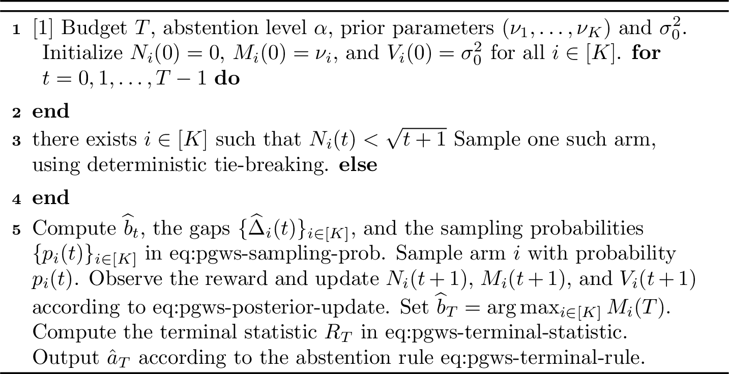
The forced-exploration step in Lines 3–4 ensures that every arm is sufficiently sampled to yield an accurate estimate of the mean. On all remaining rounds, PGWS samples arm \(i\) with probability \[\label{eq:pgws-sampling-prob} p_i(t) = \frac{\widehat\Delta_i(t)^{-2}}{\sum_{\ell=1}^K \widehat\Delta_\ell(t)^{-2}}, \qquad i\in[K].\tag{5}\] Consequently, the leader and the closest challenger receive equal sampling probability, while arms with larger posterior mean gaps receive smaller probabilities.
At the end of the sampling phase, PGWS measures the strength of the posterior evidence in favor of the final leader \(\widehat b_T\). Define \[\label{eq:pgws-terminal-statistic} R_T := \min_{j\neq \widehat b_T} \frac{ \bigl(M_{\widehat b_T}(T)-M_j(T)\bigr)^2 }{ 2\bigl(V_{\widehat b_T}(T)+V_j(T)\bigr) },\tag{6}\] which represents the smallest pairwise posterior Gaussian exponent separating the final leader from its challengers. A small value of \(R_T\) indicates that at least one challenger remains statistically difficult to be distinguished from the leader.
To calibrate abstention, let \(r_{T,\alpha}\) be the lower \(\alpha\)-quantile of \(R_T\) under the joint Bayesian law induced by the sampling rule, i.e., \[\label{equ:terminal95threshold} r_{T,\alpha} := \inf\bigl\{ r\ge 0: \mathbb{P}(R_T\le r)\ge \alpha \bigr\}.\tag{7}\] If the distribution of \(R_T\) has an atom at the threshold, define \[\label{eq:pgws-boundary-randomization} \theta_{T,\alpha} := \begin{cases} \displaystyle \frac{ \alpha-\mathbb{P}(R_T<r_{T,\alpha}) }{ \mathbb{P}(R_T=r_{T,\alpha}) }, & \mathbb{P}(R_T=r_{T,\alpha})>0,\\ 0, & \mathbb{P}(R_T=r_{T,\alpha})=0. \end{cases}\tag{8}\] The terminal decision is \[\label{eq:pgws-terminal-rule} \hat{a}_T = \begin{cases} ?, & R_T<r_{T,\alpha},\\ ?, & R_T=r_{T,\alpha} \text{ with probability } \theta_{T,\alpha},\\ \widehat b_T, & \text{otherwise}. \end{cases}\tag{9}\] Thus PGWS abstains on the least confident posterior histories, up to boundary randomization which is used only to obtain exact calibration when \(R_T\) has an atom at its \(\alpha\)-quantile.
The quantile \(r_{T,\alpha}\) is deterministic once the prior, the sampling rule, \(T\), and \(\alpha\) are fixed. For the purpose of implementation, it can be estimated offline by Monte Carlo simulation from the prior. A large-\(T\), small-\(\alpha\) approximation is \(r_{T,\alpha}^{\mathrm{asy}} = \frac{1}{8\kappa_\nu^2}\alpha^2T .\)
2.2 Upper Bound Analysis↩︎
We now derive theoretical guarantees for PGWS. In this subsection, all probabilities are under the joint Bayesian law induced by Algorithm 1.
Theorem 1 (Upper Bound for PGWS). For any \(T\) and any \(\alpha\in(0,1)\), PGWS(\(\alpha\)) with the terminal rule 9 satisfies \(\mathcal{A}_T({\textrm{\mathrm{\small PGWS}}}(\alpha))=\alpha\). Furthermore, asymptotically, \[\limsup_{\alpha\downarrow0} \limsup_{T\to\infty} \frac{1}{\alpha^2T}\log \mathcal{E}_T({\textrm{\mathrm{\small PGWS}}}(\alpha)) \le - \frac{1}{8\kappa_\nu^2}.\label{eqn:ub}\qquad{(1)}\]
The proof uses two key lemmas. In particular, the first lemma gives a finite-sample posterior certification bound: conditional on the sampled arms and observed rewards up to time step \(T\), the statistic \(R_T\) controls the posterior probability that the final leader is not the true best arm.
Lemma 1 (Posterior Certification Error Bound). For every \(T\) and every \(\alpha\in(0,1)\), \[\mathcal{E}_T({\textrm{\mathrm{\small PGWS}}}(\alpha)) \le (K-1)e^{-r_{T,\alpha}}.\]
Lemma 2 (Asymptotic Lower Bound on the Calibration Threshold). For every \(\varepsilon\in(0,1)\), there exists \(\alpha_0>0\) such that for every \(0<\alpha\le \alpha_0\), there exists \(T_0(\alpha,\varepsilon)\) such that for all \(T\ge T_0(\alpha,\varepsilon)\), \[r_{T,\alpha} \ge (1-\varepsilon) \frac{1}{8\kappa_\nu^2} \alpha^2T.\]
The proofs of both Lemmas are deferred to Appendix 8.
Proof of Theorem 1. By the definition of the lower \(\alpha\)-quantile, \(\mathbb{P}(R_T<r_{T,\alpha}) \le \alpha \le \mathbb{P}(R_T\le r_{T,\alpha}).\) The boundary randomization in 9 is chosen so that \(\mathbb{P}(\hat{a}_T=?) = \mathbb{P}(R_T<r_{T,\alpha}) + \theta_{T,\alpha}\mathbb{P}(R_T=r_{T,\alpha}) = \alpha.\) Thus \(\mathcal{A}_T({\textrm{\mathrm{\small PGWS}}}(\alpha))=\alpha\).
For the error probability, Lemma 1 gives \(\mathcal{E}_T({\textrm{\mathrm{\small PGWS}}}(\alpha)) \le (K-1)e^{-r_{T,\alpha}}.\) By Lemma 2, for every \(\varepsilon\in(0,1)\), all sufficiently small \(\alpha\), and all sufficiently large \(T\), \(r_{T,\alpha} \ge (1-\varepsilon) \frac{1}{8\kappa_\nu^2}\alpha^2T.\) Therefore \[\mathcal{E}_T({\textrm{\mathrm{\small PGWS}}}(\alpha)) \le (K-1) \exp \left\{ -(1-\varepsilon) \frac{1}{8\kappa_\nu^2}\alpha^2T \right\}.\] This then yields the final result in ?? . ◻
3 Lower Bounds↩︎
This section presents three lower bounds. The first is the main impossibility result for Bayesian BAI with abstention and matches the upper bound presented in Section 2.2. The second shows that forced-decision Bayesian BAI has only polynomial decay in the error probability, which refines the lower bound established by [14]. The third considers the frequentist (non-Bayesian) formulation and shows that, when the instance has a positive gap, abstention improves only lower-order exponential terms. Together, these results identify both the value of abstention and the role of the Bayesian formulation.
3.1 Bayesian BAI with Abstention↩︎
Theorem 2 (Lower Bound for Bayesian BAI with Abstention). In the Gaussian prior and Gaussian reward model, \[\liminf_{\alpha\downarrow0} \liminf_{T\to\infty} \frac{1}{\alpha^2T} \log \mathfrak E_{T}(\alpha) \ge -\frac{1}{8\kappa_\nu^2}.\]
Theorem 2 applies to every adaptive sampling and terminal decision rule satisfying the abstention constraint \(\mathcal{A}_T(\pi)\le\alpha\). The proof, which is deferred to Appendix 9, proceeds by decomposing the parameter space into disjoint regions \(\Omega_{ij}\) where arms \(i\) and \(j\) are the two arms with the largest means. Since the undetected error is dominated by near-tie instances, we focus on small neighborhoods of the tie surfaces inside these regions and introduce a locally flat subprior that is a submeasure of the original prior. This reduction transforms the problem into a two-arm hypothesis testing problem under a convenient approximately uniform prior. Combining a Neyman–Pearson-like argument with the aggregation over all pairs yields the exponent \(1/(8\kappa_\nu^2)\) that matches that of the upper bound.
Combining Theorem 2 with the achievability guarantee for PGWS gives the tight asymptotics on the exponential scale:
Corollary 1 (Tight Asymptotics and Optimality of PGWS). The following holds: \[\label{equ:tightness} \limsup_{\alpha\downarrow0} \limsup_{T\to\infty} \frac{1}{\alpha^2T} \log \mathcal{E}_{T}({\textrm{\mathrm{\small PGWS}}}(\alpha)) =\liminf_{\alpha\downarrow0} \liminf_{T\to\infty} \frac{1}{\alpha^2T} \log \mathfrak E_{T}(\alpha) = - \frac{1}{8\kappa_\nu^2}.\qquad{(2)}\]
Corollary 1 identifies \(\kappa_\nu\), the density at zero of the prior top-two gap \(\Gamma\), as the prior-dependent hardness parameter on the leading exponential scale.
3.2 Bayesian BAI without Abstention↩︎
To characterize the role of the abstention formulation, we next consider the forced-decision Bayesian BAI problem [14], in which the learner must recommend an arm at the end of the experiment. Recall that we defined the forced-decision Bayes error probability as in 2 . The following theorem shows that, without abstention, the Bayes probability of misidentification cannot decay exponentially fast.
Theorem 3 (No-Abstention Lower Bound). For the Gaussian prior and Gaussian reward model, \[\liminf_{T\to\infty} \sqrt T\,\mathfrak E_{T}(0) \ge \sqrt{\frac{2}{\pi}}\,\kappa_\nu.\]
The proof is deferred to Appendix 10. Theorem 3 refines the two-arm Bayesian fixed-budget BAI lower bound of [14]. They show that, for \(K=2\) Gaussian arms with Gaussian priors, the Bayes probability of misidentification is \(\Omega((T\log T)^{-1/2})\), with the multiplicative factor depending on the prior as \(\exp\big\{\!-\!\frac{(\nu_1-\nu_2)^2}{4\sigma_0^2} \big\}\). For \(K=2\), our hardness parameter is \(\kappa_\nu = 2\int_{\mathbb{R}}f_1(x)f_2(x)\,\mathrm{d}x = \frac{1}{\sigma_0\sqrt{\pi}} \exp \big\{ \!-\!\frac{(\nu_1-\nu_2)^2}{4\sigma_0^2} \big\}\). Thus Theorem 3 improves the dependence on \(T\), recovers the same prior-separation dependence through \(\kappa_\nu\), and extends the result from two arms to general \(K\ge 2\). For \(K>2\), \(\kappa_\nu\) represents a weighted sum (with weights \(\{w_{ij}\}\)) over all distinct pairs of arms \((i,j)\) of the likelihood of \(i\) and \(j\) being equal. Additionally, this theorem is also materially different from the lower bound analysis of the Bayesian simple regret in [15]. That work studies the simple regret, rather than the probability of error, and establishes a decay rate of \(\Theta(T^{-1})\).
Theorem 3 identifies the mechanism behind the polynomial Bayes error probability in standard forced-decision Bayesian FB-BAI. The dominant error comes from instances whose top-two gap, \(\Gamma=\mu_{(1)}-\mu_{(2)}\), is of order \(T^{-1/2}\). The prior probability of these instances is of order \(\kappa_\nu/\sqrt T\), and on these instances, the two leading arms cannot be reliably separated with \(T\) samples. Thus the same local near-tie density \(\kappa_\nu\) that governs the abstention exponent also determines the constant in the forced-decision problem.
This contrasts with the results for Bayesian BAI with abstention in Theorem 2. By allowing an \(\alpha\)-fraction of inconclusive decisions on the most ambiguous posterior histories, the learner removes the near-tie region that dominates the forced-decision error probability. Consequently, the error probability exhibits a fundamental phase transition from polynomial decay (i.e., \(\Omega(T^{-1/2})\)) to exponential decay (i.e., \(\exp( - \Theta( \alpha^2T) )\)).
3.3 Frequentist BAI with Abstention↩︎
The preceding results concern the Bayesian formulation, where the error probability is averaged over a prior. We now contrast this behavior with the frequentist (fixed-instance) setting, and we show that the polynomial-to-exponential improvement is specific to the Bayesian formulation. In particular, for a fixed positive-gap instance, the error probability of ordinary frequentist FB-BAI decays exponentially with \(T\) [1], [3], [4]. We show that the terminal abstention can improve only lower-order (i.e., sublinear in \(T\)) terms in the exponent.
We exemplify this point with a symmetric pair of two-arm Gaussian instances which we call the mirror experiments. Pulling arm \(i\in\{1,2\}\) produces an independent reward from \(\mathcal{N}(\mu_i,1)\). A strategy \(\pi\) adaptively samples the arms for \(T\) rounds and then outputs \(\hat{a}_T\in\{1,2,?\}\), where \(?\) denotes abstention. For an instance \(\mu\), let \(a^\star(\mu)=\arg\max_{i\in\{1,2\}}\mu_i\) be the optimal arm, and define \[\mathcal{E}_{T,\mu}(\pi) := \mathbb{P}_\mu^\pi\!\left( \hat{a}_T\notin \{a^\star(\mu),?\} \right), \quadand\quad \mathcal{A}_{T,\mu}(\pi) := \mathbb{P}_\mu^\pi(\hat{a}_T=?).\] For \(\alpha\in(0,1)\), let \[\Pi_T^{\rm freq}(\alpha) := \left\{ \pi: \sup_{\mu\in\mathbb{R}^2} \mathcal{A}_{T,\mu}(\pi)\le \alpha \right\}\] be the class of strategies with abstention probability uniformly bounded above by \(\alpha\). Let \(z_\alpha := \Phi^{-1}\!\left(\frac{1+\alpha}{2}\right)\), so that \(\mathbb{P}(|Z|\le z_\alpha)=\alpha\) for \(Z\sim\mathcal{N}(0,1)\).
Fix \(x\in\mathbb{R}\) and \(\Delta>0\), and consider the following two mirror instances \[\mu^+ := \left( x+\frac{\Delta}{2}, x-\frac{\Delta}{2} \right), \quadand\quad \mu^- := \left( x-\frac{\Delta}{2}, x+\frac{\Delta}{2} \right).\] Under \(\mu^+\), arm \(1\) is optimal; under \(\mu^-\), arm \(2\) is optimal.
Theorem 4 (Two-Arm Frequentist Lower Bound with Abstention). Given \(T\in\mathbb{N}\), \(\alpha\in(0,1)\), \(x\in\mathbb{R}\), \(\Delta>0\), and any strategy \(\pi\in\Pi_T^{\rm freq}(\alpha)\), we have \[\max\left\{ \mathcal{E}_{T,\mu^+}(\pi), \mathcal{E}_{T,\mu^-}(\pi) \right\} \ge \Phi\!\left( -\frac{\Delta\sqrt T}{2}-z_\alpha \right).\]
The proof is deferred to Appendix 11. The theorem is a minimax statement over the mirror instances \((\mu^+,\mu^-)\): any strategy whose abstention probability is uniformly bounded by \(\alpha\) necessarily incurs the stated undetected error on at least one of the two instances.
This bound is sharp for the two-arm Gaussian mirror experiment: when \(T\) is even, sampling each arm \(T/2\) times and abstaining when \(|\hat{\mu}_1-\hat{\mu}_2|\le \frac{2z_\alpha}{\sqrt T}\) attains the lower bound.
Theorem 4 shows that abstention does not change the leading fixed-gap exponential rate. Without abstention, the policy that pulls each arm an equal number of times results in the error probability \[\Phi\!\left(-\frac{\Delta\sqrt T}{2}\right) = \exp\!\left\{ -\frac{\Delta^2}{8}T+O(\log T) \right\}.\] With an abstention budget \(\alpha\), the undetected error probability becomes \[\Phi\!\left( -\frac{\Delta\sqrt T}{2}-z_\alpha \right) = \exp\!\left\{ -\frac{\Delta^2}{8}T -\frac{\Delta z_\alpha}{2}\sqrt T -\frac{z_\alpha^2}{2} +O(\log T) \right\}.\] Hence, abstention only improves the exponent by a lower order term. For small \(\alpha\), \(z_\alpha=\sqrt{\pi/2}\,\alpha+O(\alpha^3)\), so the logarithmic improvement is of order \(O(\alpha\sqrt T)\). In contrast to the Bayesian formulation, the error probability under the frequentist setup is already decaying exponentially without abstention, and the additional option to abstain yields only a lower-order improvement in the error probability, characterized by a moderate-deviation term.
4 Extensions Beyond the Gaussian Model↩︎
In the preceding sections, we established the polynomial-to-exponential phase transition under the Gaussian model. In this section, we show that this transition extends beyond the Gaussian setting. Specifically, the same exponent arises for regular one-parameter reward models after measuring gaps in the Fisher–Rao information scale.
Let \(\mathcal{I}\subseteq\mathbb{R}\) be an open interval, called the quality parameter space. At the beginning of each experiment, the quality parameters \(\mu_1,\ldots,\mu_K\in\mathcal{I}\) are drawn from their prior distributions and remain fixed throughout the experiment. The best arm is \(a^\star:=\arg\max_{i\in[K]}\mu_i\). Conditional on \(\mu_1, \ldots, \mu_K\), each pull of arm \(i\) produces an independent reward with distribution \(P_{\mu_i}\). We assume that each \(P_{\mu_i}\) comes from a regular one-parameter exponential family, defined as follows.
assumptionAssRegularExpfam The family \(\{P_\mu: \mu\in\mathcal{I}\}\) is a regular full one-parameter exponential family, possibly after a smooth monotone reparameterization (which we call \(\theta(\cdot)\)); see, e.g., [6]. Specifically, there exists an open natural parameter space \(\Theta\subseteq\mathbb{R}\), a dominating measure \(\lambda\), a natural statistic \(t(\cdot)\), a base distribution \(h(\cdot)\), a \(C^4\) log-partition function \(A:\Theta\to\mathbb{R}\) with \(A''(\theta)>0\), and a \(C^4\) map \(\theta:\mathcal{I}\to\Theta\) onto \(\Theta\) with \(\theta'(\mu)>0\) such that \(\theta(\mu)\) is the natural parameter corresponding to the quality parameter \(\mu\), and \[\frac{\mathrm{d}P_\mu}{\mathrm{d}\lambda}(w) = h(w)\exp\big\{ \theta(\mu)t(w)-A(\theta(\mu)) \big\}, \qquad \mu\in\mathcal{I} .\] Moreover, the image of every compact subset of \(\mathcal{I}\) under \(\theta\) is compact in \(\Theta\).
Under Assumption [ass:regular-expfam], the Fisher information for the quality parameter \(\mu\) is \[I(\mu) := A''(\theta(\mu))\big(\theta'(\mu)\big)^2 .\] We then define the Fisher–Rao information coordinate \[s(\mu) := \int_{\mu_\circ}^{\mu}\sqrt{I(v)}\,\mathrm{d}v, \label{eqn:fisher95rao}\tag{10}\] where \(\mu_\circ\in\mathcal{I}\) is arbitrary and all quantities and results below are independent of the choice of \(\mu_\circ\), as changing \(\mu_\circ\) shifts \(s(\cdot)\) by an additive constant, leaving \(\kappa\) and gap-based results unchanged. This is the arc-length coordinate induced by the Fisher–Rao metric [27], [28]. Since \(s(\cdot)\) is strictly increasing, the best arm is unchanged by the transformation \(\mu_i\mapsto \eta_i:=s(\mu_i)\).
assumptionAssRegularInfoPrior The arms’ quality parameters \(\mu_1,\ldots,\mu_K\) are independent under the prior. In the information coordinate \(\eta_i=s(\mu_i)\), the induced prior distribution of arm \(i\) has density \(\bar f_i\) and distribution function \(\bar F_i\) on \(\mathcal{H}:=s(\mathcal{I})\). For each \(i\in[K]\), \[\bar f_i \text{ is continuous and bounded on }\mathcal{H}, \qquad \bar f_i(\eta)>0 \quad \forall\, \eta\in\mathcal{H} .\]
Define the information-scaled top-two tie density \[\kappa := \sum_{i\neq j} \int_{\mathcal{H}} \bar f_i(u)\bar f_j(u) \prod_{k\neq i,j}\bar F_k(u) \,\mathrm{d}u .\] Equivalently, if \(f_i\) and \(F_i\) respectively denote the prior density and distribution function of \(\mu_i\) in the original coordinate system, then \[\kappa = \sum_{i\neq j} \int_{\mathcal{I}} \frac{ f_i(\mu)f_j(\mu)\prod_{k\neq i,j}F_k(\mu) }{\sqrt{I(\mu)}} \,\mathrm{d}\mu .\] Thus \(\kappa\) is the density at zero of the top-two gap after transforming the quality parameters to Fisher–Rao coordinates via 10 . In the Gaussian model with unit variance, \(\theta(\mu)\equiv\mu\) and \(I(\mu)\equiv1\), so this reduces to the top-two gap density used in the preceding sections.
For the achievability result we also assume a global quadratic lower bound on the Kullback–Leibler (KL) divergence. Let \(D(\mu,z):=D(P_\mu\,\|\,P_z) .\)
assumptionAssQuadraticKL There exists \(c_{\rm KL}>0\) such that, for all \(\mu,z\in\mathcal{I}\), \[D(\mu,z) \ge c_{\rm KL}\big(s(\mu)-s(z)\big)^2 . \label{eqn:quad95growth}\tag{11}\]
Assumption [ass:quadratic-kl] holds for several one-parameter exponential families when \(s(\cdot)\) is the Fisher–Rao information coordinate. In particular, Gaussians with unit variance, Bernoulli, and Poisson satisfy 11 with \(c_{\rm KL}=1/4\). Assumption [ass:quadratic-kl] can be viewed as a global version of the local quadratic approximation \(D(\mu,z)\approx\frac{1}{2}\big(s(\mu)-s( z)\big)^2\) where \(|s(\mu)-s( z)|\) is the Fisher–Rao distance [28].
Theorem 5 (Extension to General Distributions). Suppose Assumptions [ass:regular-expfam]–[ass:quadratic-kl] hold, then \[\limsup_{\alpha\downarrow0} \limsup_{T\to\infty} \frac{1}{\alpha^2T} \log \mathcal{E}_{T}(\text{\mathrm{\small IC-PGWS}}(\alpha)) =\liminf_{\alpha\downarrow0} \liminf_{T\to\infty} \frac{1}{\alpha^2T} \log \mathfrak E_{T}(\alpha) = -\frac{1}{8\kappa^2}.\] The lower bound holds for all adaptive policies satisfying the abstention constraint, and the upper bound is attained by an information-coordinate version of PGWS, namely, IC-PGWS.
The proof is postponed to Appendix 12. We now provide a concrete example of applying Theorem 5 to Beta-Bernoulli arms.
Example 1 (Beta–Bernoulli arms). Consider Bernoulli rewards with unknown success probabilities \(\mu_i\in(0,1)\) that follow Beta distributions, i.e., \[Y_{i,s}\mid \mu_i \sim {\rm Bernoulli}(\mu_i), \quadand\quad \mu_i\sim {\rm Beta}(a_i,b_i),\] independently across arms and time, where \(a_i,b_i\ge 1/2\) for \(i \in [K]\).
We show that the Beta–Bernoulli arms satisfy Assumptions [ass:regular-expfam]–[ass:quadratic-kl]. Firstly, the Bernoulli family is a regular exponential family with \[\theta(\mu)=\log\frac{\mu}{1-\mu}, \quad A(\theta)=\log(1+e^\theta), \quadand\quad t(w)=w .\] Its Fisher information is \(I(\mu)=\frac{1}{\mu(1-\mu)}\). Hence, \(s(\mu)= \int_0^\mu\sqrt{I(v)}\, \mathrm{d}v= 2\arcsin\sqrt{\mu}\), and \(\mathcal{H}=(0,\pi)\).
Secondly, if \(\eta=s(\mu)\), then \(\mu=\sin^2(\eta/2)\), and the prior density of \(\eta_i\) is \[\bar f_i(\eta) = \frac{ \sin^{2a_i-1}(\eta/2)\cos^{2b_i-1}(\eta/2) }{ {\rm Beta}(a_i,b_i) }, \qquad 0<\eta<\pi .\] Because \(a_i,b_i\ge1/2\), this density is bounded, continuous, and strictly positive on \((0,\pi)\). Hence, Assumption [ass:regular-info-prior] holds.
Lastly, a routine calculation shows that the Bernoulli KL divergence satisfies \[D(\mu,z) \ge \frac{1}{4}\big(s(\mu)-s(z)\big)^2, \qquad \mu,z\in(0,1),\] so Assumption [ass:quadratic-kl] also holds with \(c_{\rm KL}=1/4\).
Therefore, the conditions of Theorem 5 hold and the theorem applies. Define \[\kappa_{\rm BB} := \sum_{i\neq j} \int_0^\pi \bar f_i(u)\bar f_j(u) \prod_{k\neq i,j}\bar F_k(u) \,\mathrm{d}u = \sum_{i\neq j} \int_0^1 f_i(\mu)f_j(\mu) \prod_{k\neq i,j}F_k(\mu) \sqrt{\mu(1-\mu)} \,\mathrm{d}\mu\] where \(\bar F_i\) is the cumulative distribution function of \(2\arcsin\sqrt{\mu_i}\), and \(f_i\) and \(F_i\) are, respectively, the Beta\((a_i,b_i)\) density and CDF. So by Theorem 5, we have \[\limsup_{\alpha\downarrow0} \limsup_{T\to\infty} \frac{1}{\alpha^2T} \log \mathcal{E}_{T}^{\rm BB}(\text{\mathrm{\small IC-PGWS}}(\alpha)) =\liminf_{\alpha\downarrow0} \liminf_{T\to\infty} \frac{1}{\alpha^2T} \log \mathfrak E_{T}^{\rm BB}(\alpha) = -\frac{1}{8\kappa^2_{\rm {BB}}}.\] in the Beta-Bernoulli case.
5 Numerical Experiments↩︎
We conduct numerical experiments to illustrate the benefit brought by the abstention option and the superior design of the sampling rule in PGWS. First, we evaluate the practical benefit of abstention by comparing the undetected error probability for several abstention levels. Second, we isolate the value of the PGWS allocation by comparing it with uniform allocation under the same posterior abstention threshold.
5.1 Experimental Setup↩︎
We adopt the Gaussian prior and reward model from Section 1.2. The prior is \(\mu_i\sim \mathcal{N}(\nu_i,\sigma_0^2)\) for \(i\in[K]\), independently across arms, and rewards satisfy \(Y_{i,s}\mid \mu_i\sim \mathcal{N}(\mu_i,1)\). We consider the arm prior with \(K=5\), \(\sigma_0=1\), and \(\nu=[5,5,3,3,2]\). The following methods are involved in the comparison:
PGWS\((\alpha)\): PGWS with the quantile-calibrated posterior abstention threshold \(\widehat r_{T,\alpha}\), so that the abstention probability is \(\alpha\).
Unif\((\alpha)\): Uniform allocation, followed by recommending the posterior leader. Use the same terminal statistic and calibration procedure as PGWS.
BayesElim [14]: Bayesian elimination without abstention, used as a forced-decision Bayesian BAI baseline.
For PGWS\((\alpha)\) and Unif\((\alpha)\), the abstention threshold is calibrated separately for each sampling rule, budget \(T\), so that the abstention probability is upper bounded by \(\alpha\). Specifically, the abstention threshold is the lower \(\alpha\)-quantile \(r_{T,\alpha}\) defined in 7 . For PGWS\((\alpha)\), for each given budget \(T\) and abstention level \(\alpha\), we apply the given sampling rule and generate terminal statistic samples \(\{R_{T}^{(m)}\}_{m\in [M_{\rm cal}]}\) of independent \(M_{\rm cal}=10^5\) simulations from the prior. We approximate the abstention threshold \(r_{T,\alpha}\) by its empirical estimate \[\widehat r_{T,\alpha} := \min\left\{ r: \frac{1}{M_{\rm cal}} \sum_{m=1}^{M_{\rm cal}} \mathbb{1}\{R_T^{(m)}\le r\} \ge \alpha \right\}.\] For \(\alpha=0\), there is no abstention and the algorithm always recommends the posterior mean leader.
The performance is evaluated on an independent test sample of \(M_{\rm test}=10^6\) prior-generated experiments. For each method, budget \(T\), and abstention level \(\alpha\), we compute the empirical abstention probability and empirical undetected error probability as follows: \[\widehat{\mathcal{A}}_T := \frac{1}{M_{\rm test}} \sum_{m=1}^{M_{\rm test}} \mathbb{1}\big\{\hat{a}_T^{(m)}=?\big\} ,\quad and \quad \widehat{\mathcal{E}}_T := \frac{1}{M_{\rm test}} \sum_{m=1}^{M_{\rm test}} \mathbb{1}\big\{ \hat{a}_T^{(m)}\notin\{a^{\star,(m)},?\} \big\},\] where \(a^{\star,(m)}\) denotes the true best arm in the \(m\)th prior-generated experiment, and \(\hat{a}_T^{(m)}\in[K]\cup\{?\}\) is the terminal output of the algorithm.
5.2 Effect of Abstention↩︎
In the first experiment, we aim to demonstrate the value of abstention. We run PGWS\((\alpha)\) for \(\alpha\in\{0,0.01,0.03,0.05\}\) over a range of budgets \(T\), and report the empirical undetected error probability \(\widehat{\mathcal{E}}_T\). The empirical abstention rate \(\widehat{\mathcal{A}}_T\) is reported separately to verify the correctness of threshold calibration. The results are shown in Figure 2:
Significant reduction in undetected error probability (Figure 2 (a)): The forced-decision baselines (PGWS\((0)\) and BayesElim [14]) exhibit a significantly slower decay in the error probability compared to the case where abstention is allowed, i.e., PGWS\((\alpha)\) for positive \(\alpha\). This corroborates our main result in Theorem 1: spending a small fraction of inconclusive decisions on the most ambiguous instances yields an exponential reduction in terminal misidentifications. In addition, Figure 2 (a) also shows that the curves for PGWS\((\alpha)\) when \(\alpha\) is positive are approximately affine, demonstrating exponential decay in the undetected error probability.
Abstention calibration (Figure 2 (b)): Across all budgets \(T\), PGWS\((\alpha)\) adheres to the prescribed abstention targets without being overly conservative. This validates the practical reliability of our calibrated abstention threshold.
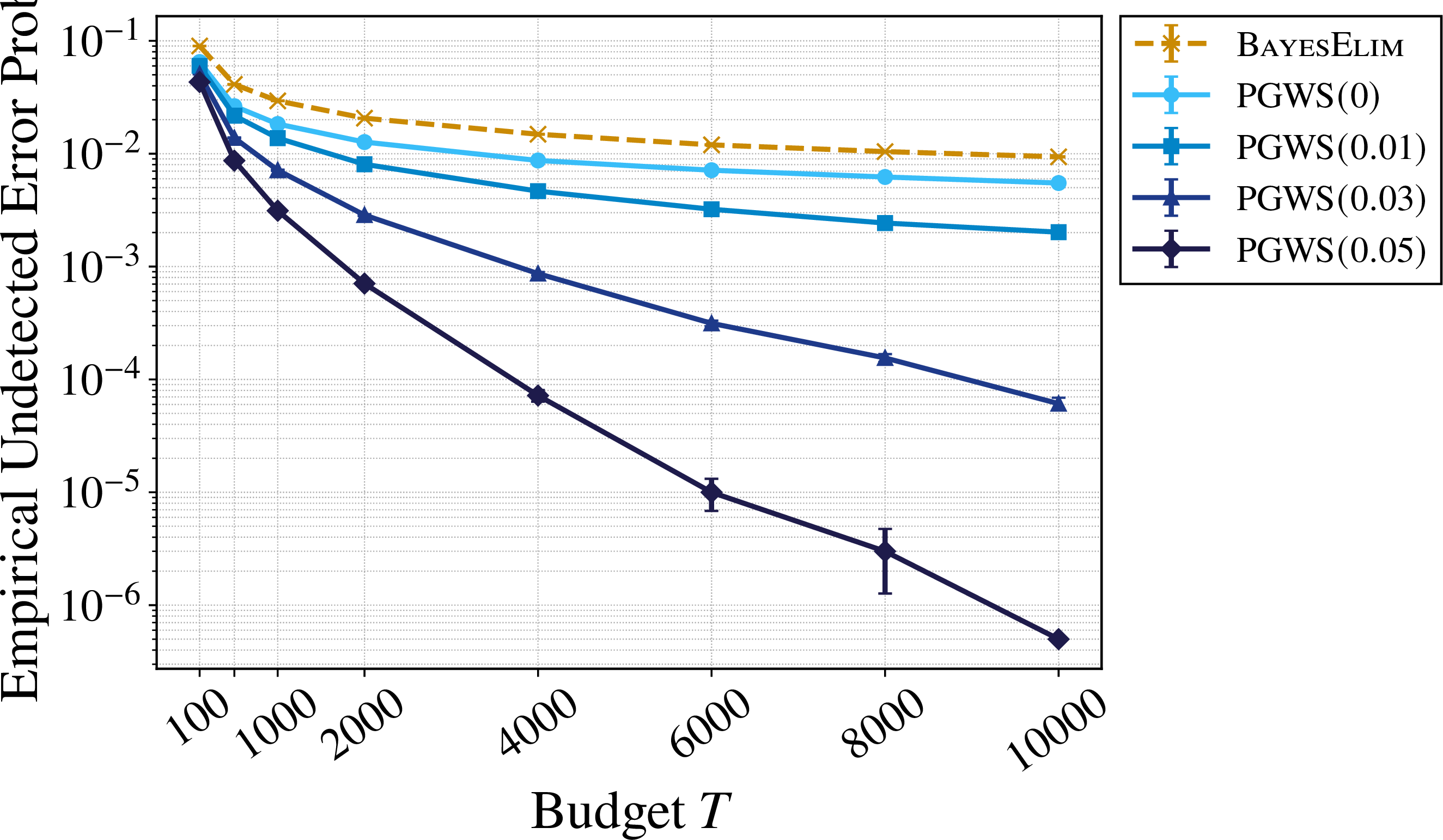
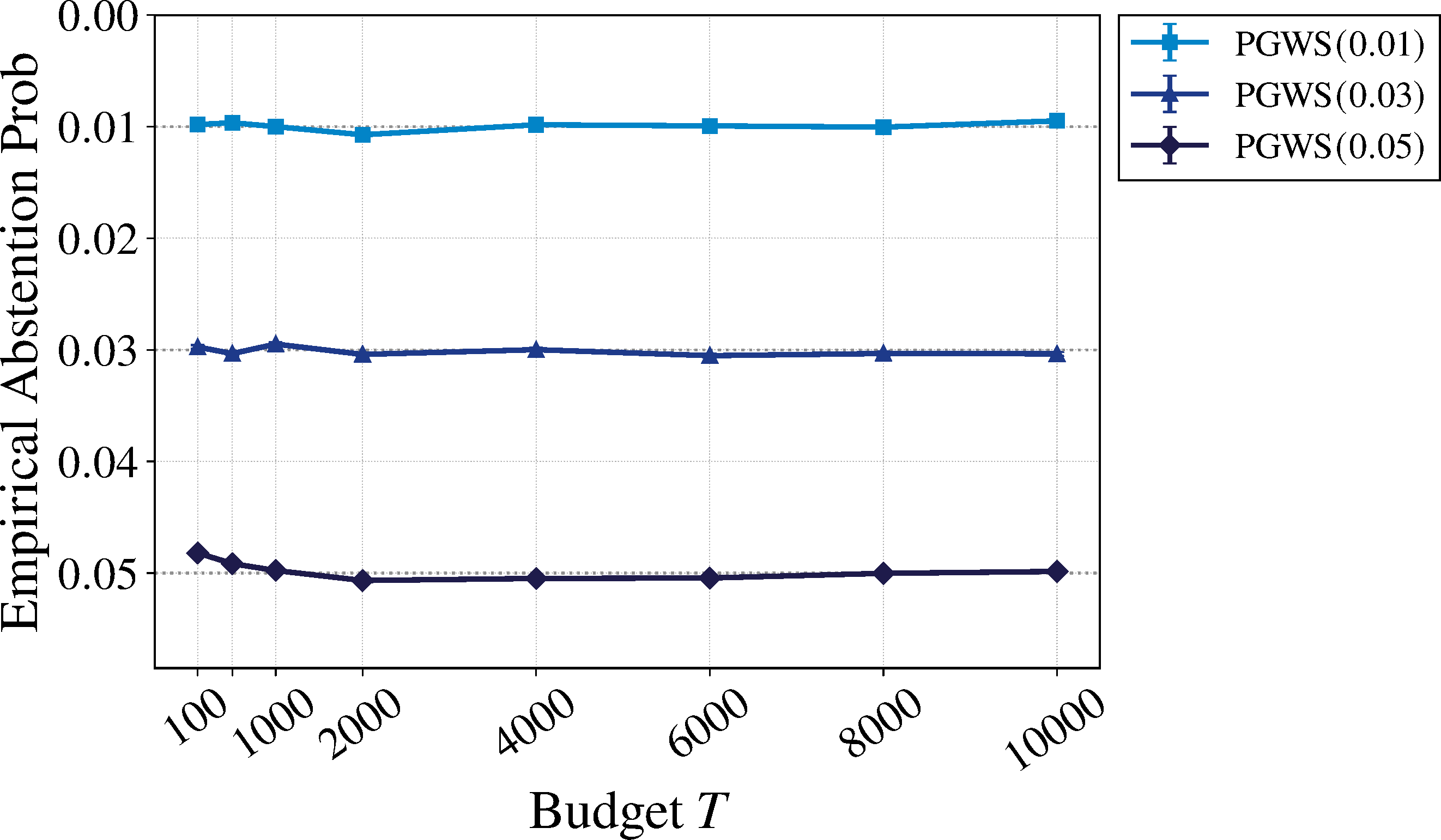
Figure 2: Plots of the undetected and abstention probabilities as functions of the budget \(T\). a — \(\widehat{\mathcal{E}}_T\) against \(T\), b — \(\widehat{\mathcal{A}}_T\) against \(T\)
5.3 Effect of Adaptive Sampling in PGWS↩︎
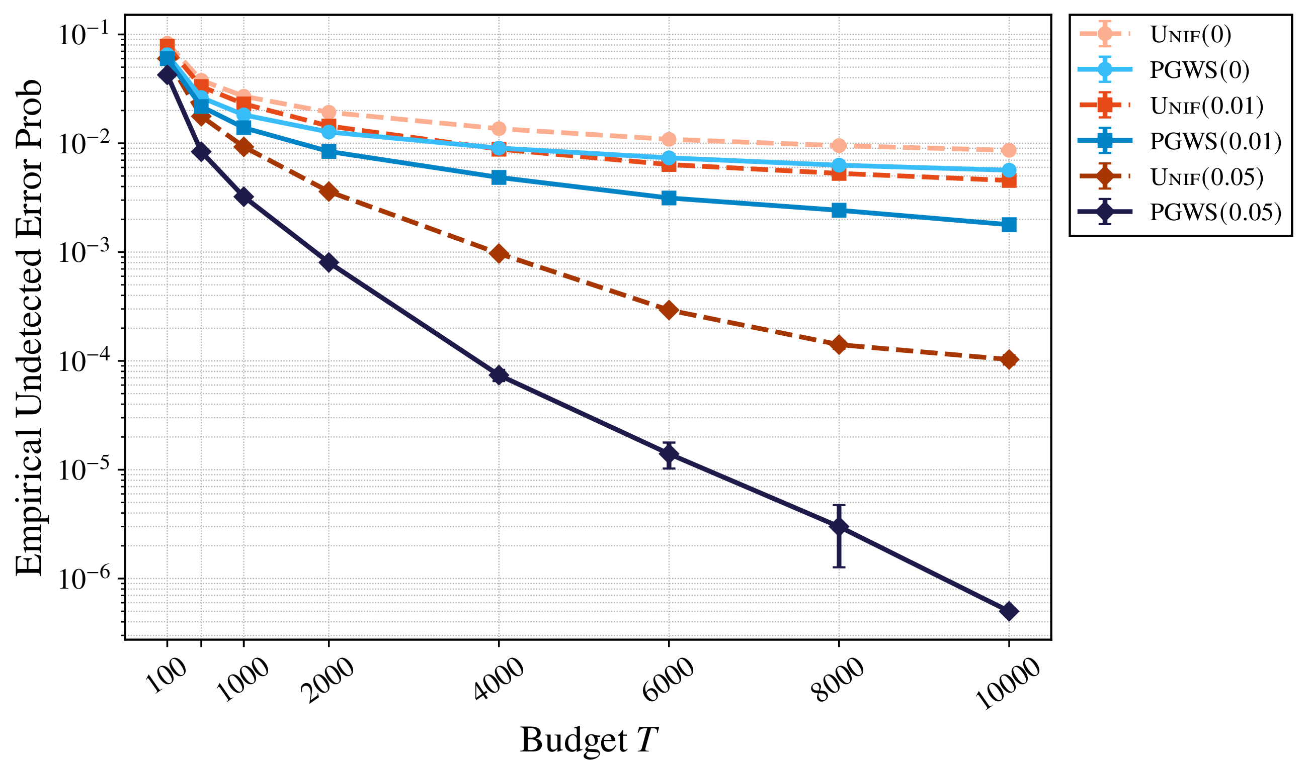
The second experiment illustrates the effectiveness of the sampling strategy of PGWS as in 5 , which adapts to the instance. We compare PGWS\((\alpha)\) with uniform allocation Unif\((\alpha)\) for the abstention levels \(\alpha\in\{0,0.01,0.05\}\), and the results are shown in Figure 3. We observe that for every abstention level, PGWS\((\alpha)\) achieves a significantly lower undetected error probability than Unif\((\alpha)\) across all budgets. The performance gap highlights the practical superiority of our algorithm’s adaptive sampling design. By dynamically concentrating the sampling budget on the posterior mean leader and its most relevant challengers, rather than wasting pulls uniformly across all arms, the algorithm more efficiently resolves the ambiguous near-tie instances that dominate the Bayes error probability.
6 Conclusion↩︎
In this paper, we studied Bayesian FB-BAI with an abstention option. We characterized the sharp small-abstention, large-budget exponent: \[\mathfrak E_{T}(\alpha) = \exp\!\left\{ -\frac{\alpha^2T}{8\kappa_\nu^2} +o(\alpha^2T) \right\}.\] The exponent is governed by the density \(\kappa_\nu\) of the prior top-two gap at zero.
We proposed PGWS, an adaptive algorithm that allocates samples to the posterior mean leader and its challengers. PGWS samples arms according to the empirical allocation distribution which is proportional to the reciprocal of the squared posterior mean gaps. It achieves the same exponent as the information-theoretic lower bound. Hence it is asymptotically optimal on the \(\alpha^2T\) logarithmic scale. Numerical experiments support the practicality of our theoretical findings.
Our results clarify the benefits of abstention. Without abstention, Bayesian BAI has only a polynomial error decay, driven by prior probability on instances with top-two gap of order \(T^{-1/2}\). With abstention, the learner can spend its abstention budget on these near-tie instances, leading to exponentially decaying undetected error. In contrast, in the frequentist fixed-gap setting, ordinary BAI is already exponentially accurate, and abstention improves only lower-order terms in the exponent.
Finally, we showed that the same mechanism extends beyond the Gaussian model under continuous prior, one parameter exponential family reward, and quadratic KL growth conditions, with the Gaussian top-two gap density replaced by an information-scaled top-two gap density.
Appendix
7 Prior Density of the Top-Two Gap at Zero↩︎
Lemma 3 (Prior Density of the Top-Two Gap at Zero). The hardness parameter \(\kappa_\nu\) and the top-two gap \(\Gamma\) are related as follows: \[\kappa_\nu = \lim_{\varepsilon\downarrow0} \frac{\mathbb{P}_\nu(\Gamma\le \varepsilon)}{\varepsilon}.\]
Proof. For each arm \(i \in [K]\), the event that arm \(i\) is the best and the top-two gap is at most \(\varepsilon\) is \(\left\{ \mu_i=\mu_{(1)},\; \mu_{(1)}-\mu_{(2)}\le \varepsilon \right\}.\) Conditional on \(\{\mu_i=x\}\), this event says that the means of all the other arms are at most \(x\) and at least one other arm is in \([x-\varepsilon,x]\). Hence \[\begin{align} \mathbb{P}(\Gamma\le \varepsilon) &= \sum_{i=1}^K \mathbb{P}(\mu_i=\mu_{(1)},\; \mu_{(1)}-\mu_{(2)}\le \varepsilon) =\sum_{i=1}^K \int_{\mathbb{R}} f_i(x) \left[ \prod_{k\neq i}F_k(x) - \prod_{k\neq i}F_k(x-\varepsilon) \right]\mathrm{d}x \end{align}\] Let \(G_i(x):=\prod_{k\neq i}F_k(x)\), then \(G_i'(x) = \sum_{j\neq i} \big( f_j(x)\prod_{k\neq i,j}F_k(x) \big)\). By the fundamental theorem of calculus, \(G_i(x)-G_i(x-\varepsilon) = \int_{x-\varepsilon}^x G_i'(u)\,\mathrm{d}u.\) Additionally, by the dominated convergence theorem, as \(\varepsilon \to 0\), \[\begin{align} \frac{\mathbb{P}(\Gamma\le \varepsilon)}{\varepsilon} &= \sum_{i=1}^K \int_{\mathbb{R}} f_i(x) \left[ \frac{G_i(x) - G_i(x-\varepsilon)}{\varepsilon} \right] \, \mathrm{d}x\to \sum^K_{i=1} \sum_{j\neq i} \int_{\mathbb{R}} f_i(x)f_j(x)\prod_{k\neq i,j}F_k(x)\,\mathrm{d}x. \end{align}\] It remains to simplify the product of the Gaussian densities. For \(i<j\), \[\begin{align} f_i(x)f_j(x) &= \frac{1}{2\pi\sigma_0^2} \exp\!\left( -\frac{(x-\nu_i)^2 + (x-\nu_j)^2}{2\sigma_0^2} \right) = \frac{1}{2\sqrt\pi\,\sigma_0} \exp\left( -\frac{(\nu_i-\nu_j)^2}{4\sigma_0^2} \right) g_{ij}(x), \end{align}\] where \(g_{ij}\) is the density of \(\mathcal{N}\!\left( \frac{\nu_i+\nu_j}{2}, \frac{\sigma_0^2}{2} \right)\). Therefore \[\begin{align} 2\int_{\mathbb{R}} f_i(x)f_j(x)\prod_{k\neq i,j}F_k(x)\,\mathrm{d}x &= \frac{1}{\sigma_0\sqrt\pi} \exp\!\left( -\frac{(\nu_i-\nu_j)^2}{4\sigma_0^2} \right) \int_{\mathbb{R}} g_{ij}(x)\prod_{k\neq i,j}F_k(x)\,\mathrm{d}x \\ &= \frac{1}{\sigma_0\sqrt\pi} \exp\!\left( -\frac{(\nu_i-\nu_j)^2}{4\sigma_0^2} \right) w_{ij}. \end{align}\] Summing over \(i<j\) proves the claim. ◻
8 Proof of Theorem 1↩︎
8.1 Error Guarantee↩︎
Proof of Lemma 1. If the algorithm recommends \(\widehat b_T\), then conditional on \(\mathcal{F}_T\), \[\mathbb{P}(a^\star\neq \widehat b_T\mid \mathcal{F}_T) \le \sum_{j\neq \widehat b_T} \mathbb{P}(\mu_j\ge \mu_{\widehat b_T}\mid \mathcal{F}_T).\]
As usual, let \(\mu=(\mu_1,\dots,\mu_K)\). By the independent Gaussian prior and the arm-wise reward model, the posterior factorizes across arms even under adaptive sampling: \[p(\mu\mid\mathcal{F}_T) \propto \prod_{i=1}^K \left[ p(\mu_i) \prod_{s=1}^{N_i(T)} p(Y_{i,s}\mid \mu_i) \right].\] Consequently, the law of the means is \[\mathcal{L}(\mu_1,\dots,\mu_K\mid\mathcal{F}_T) = \bigotimes_{i=1}^K \mathcal{N}(M_i(T),V_i(T)),\] thus the arm means \(\mu_1,\dots,\mu_K\) are mutually independent conditional on \(\mathcal{F}_T\).
Furthermore, \(M_i(T)\) and \(V_i(T)\) are \(\mathcal{F}_T\)-measurable, and therefore \(\widehat b_T=\arg\max_i M_i(T)\) is also \(\mathcal{F}_T\)-measurable. Hence, conditional on \(\mathcal{F}_T\), the random index \(\widehat b_T\) is fixed. Thus, for each \(j\neq \widehat b_T\), \[\mu_{\widehat b_T}-\mu_j\mid\mathcal{F}_T \sim \mathcal{N}\!\left( M_{\widehat b_T}(T)-M_j(T), V_{\widehat b_T}(T)+V_j(T) \right).\] Therefore, using \(\Phi(-x)\le e^{-x^2/2}\) for \(x\ge0\), \[\mathbb{P}(\mu_j\ge\mu_{\widehat b_T}\mid\mathcal{F}_T) = \Phi\left( -\frac{M_{\widehat b_T}(T)-M_j(T)}{\sqrt{V_{\widehat b_T}(T)+V_j(T)}} \right) \le \exp\left( -\frac{ \bigl(M_{\widehat b_T}(T)-M_j(T)\bigr)^2 }{ 2\bigl(V_{\widehat b_T}(T)+V_j(T)\bigr) } \right).\] By definition of \(R_T\), on the event that the algorithm does not abstain we have \(R_T\ge r_{T,\alpha}\). Hence, on this event, \(\mathbb{P}(a^\star\neq \widehat b_T\mid\mathcal{F}_T) \le (K-1)e^{-R_T} \le (K-1)e^{-r_{T,\alpha}}.\)
Taking expectation gives \[\mathcal{E}_T = \mathbb{E}\!\left[ \mathbb{1}\{\hat{a}_T\neq ?\} \mathbb{P}(a^\star\neq \widehat b_T\mid\mathcal{F}_T) \right] \le (K-1)e^{-r_{T,\alpha}}.\] ◻
8.2 Asymptotic Behavior of the Statistic \(R_T\)↩︎
To analyze the (asymptotic) behavior of \(r_{T,\alpha}\), we first analyze \(R_T\).
For ease of notation, we introduce auxiliary unnormalized weights. At time \(t\), define \(\widehat b_t\) and \(\widehat\Delta_i(t)\) from the posterior means as in Algorithm 1. We also define \(\widehat{\Gamma}_t = \widehat\Delta_{\widehat b_t}(t)\). Set \(w_{\widehat b_t}(t)=1\), \(w_{j}(t)=\big(\frac{\widehat{\Gamma}_t}{\widehat\Delta_j(t)}\big)^2\) for \(j \neq \widehat b_t\), and \(W(t):=\sum_{\ell=1}^K w_\ell(t)\). Then, on every non-forced round, the sampling rule in 5 in Algorithm 1 can be written equivalently as \(p_i(t)=\frac{w_i(t)}{W(t)}\) for \(i\in[K]\).
Let \(b^\star:=\arg\max_{i\in[K]}\mu_i\) be the true best arm which is unique almost surely. For \(j\neq b^\star\), define the true gap \(\Delta_j:=\mu_{b^\star}-\mu_j>0\). Recall that the true top-two gap is \(\Gamma:=\min_{j\neq b^\star}\Delta_j = \mu_{(1)}-\mu_{(2)}\).
Define the (deterministic) unnormalized limiting sampling weights \[w_{b^\star}^\dagger(\mu):=1, \quadand\quad w_j^\dagger(\mu) := \left( \frac{\Gamma}{\Delta_j} \right)^2, \qquad j\neq b^\star,\] Also define their sum, which is the normalization constant for the sampling distribution \[W^\dagger(\mu) := \sum_{\ell=1}^K w_\ell^\dagger(\mu) = 1+\sum_{j\neq b^\star} \left( \frac{\Gamma}{\Delta_j} \right)^2. \label{eqn:W95dagger}\tag{12}\] Finally, define the limiting sampling proportions \[p_i^\dagger(\mu) := \frac{w_i^\dagger(\mu)}{W^\dagger(\mu)} = \frac{w_i^\dagger(\mu)}{\sum_{\ell=1}^K w_\ell^\dagger(\mu)},\] as well as the worst-case pairwise error exponent \[C^\dagger(\mu) := \min_{j\neq b^\star} \frac{ \Delta_j^2 }{ 2\left( 1/p_{b^\star}^\dagger(\mu)+1/p_j^\dagger(\mu) \right) }.\]
Next we simplify \(C^\dagger(\mu)\).
Lemma 4 (Explicit Form of the Limiting Exponent). Almost surely, \[C^\dagger(\mu) = \frac{\Gamma^2}{4W^\dagger(\mu)}.\] In particular, \[\frac{\Gamma^2}{4K} \le C^\dagger(\mu) \le \frac{\Gamma^2}{8}.\]
Proof. By definition, the normalized sampling proportions are: \[p_{b^\star}^\dagger=\frac{1}{W^\dagger(\mu)}, \quadand\quad p_j^\dagger = \frac{\Gamma^2/\Delta_j^2}{W^\dagger(\mu)}.\] We substitute these proportions into the pairwise error exponent for a specific challenger \(j\): \[\frac{ \Delta_j^2 }{ 2\left( 1/p_{b^\star}^\dagger+1/p_j^\dagger \right) } = \frac{ \Delta_j^2 }{ 2W^\dagger(\mu)\left(1+\Delta_j^2/\Gamma^2\right) }.\] To isolate the effect of the gap, we factor out \(\frac{\Gamma^2}{2W^\dagger(\mu)}\) and express the remainder as a function of the relative gap \(r_j := \Delta_j/\Gamma\): \[\frac{ \Delta_j^2 }{ 2\left( 1/p_{b^\star}^\dagger+1/p_j^\dagger \right) } = \frac{\Gamma^2}{2W^\dagger(\mu)} \left[ \frac{(\Delta_j/\Gamma)^2}{1+(\Delta_j/\Gamma)^2} \right] = \frac{\Gamma^2}{2W^\dagger(\mu)} \left( \frac{r_j^2}{1+r_j^2} \right).\]
Now, recall the limiting exponent \(C^\dagger(\mu)\) is defined as the minimum of this expression over all challengers \(j \neq b^\star\). Observe that the function \(f(r) = \frac{r^2}{1+r^2}\) is increasing on \([1,\infty)\). Since \(\Delta_j/\Gamma\ge1\) for all \(j\neq b^\star\), the minimum is attained by a second-best arm, for which \(\Delta_j=\Gamma\): \[C^\dagger(\mu) = \frac{\Gamma^2}{2W^\dagger(\mu)} \left( \frac{1^2}{1+1^2} \right) = \frac{\Gamma^2}{4W^\dagger(\mu)}.\] Also, because \(w_{b^\star}^\dagger=1\), the second-best arm has weight \(1\), and all other weights are at most \(1\), we have \(2\le W^\dagger(\mu)\le K\). Substituting back gives \[\frac{\Gamma^2}{4K} \le C^\dagger(\mu) \le \frac{\Gamma^2}{8}.\] ◻
Next, we prove that the forced-exploration safeguard collects enough data to guarantee the posterior mean of every arm converges to its true mean.
Lemma 5 (Posterior Consistency). For every arm \(i\), \[M_i(t)\to \mu_i \qquad\text{almost surely}. \label{eqn:Mit95as}\qquad{(3)}\]
Proof. First, recall that the algorithm’s forced-exploration samples arm \(i\) whenever \(N_i(t) < \sqrt{t+1}\), this guarantees that as \(t \to \infty\), \(N_i(t)\to\infty\) for every \(i\).
Second, conditional on a specific realization of the true mean \(\mu_i\), the reward sequence \((Y_{i,s})_{s\ge1}\) consists of mutually independent draws from \(\mathcal{N}(\mu_i,1)\). Therefore, by the Strong Law of Large Numbers, the conditional probability of the empirical average converging to \(\mu_i\) is \(1\). Integrating this over the prior of \(\mu_i\), we have \[\frac{1}{N_i(t)} \sum_{s=1}^{N_i(t)}Y_{i,s} \to \mu_i \qquad\text{almost surely}.\]
Finally, recall our algorithm’s update for the posterior mean: \[M_i(t) = \frac{ \sigma_0^{-2}\nu_i+\sum_{s=1}^{N_i(t)}Y_{i,s} }{ \sigma_0^{-2}+N_i(t) }.\] Combining the previous two displayed equations yields ?? . ◻
Next, we show that the empirical allocation of arm pulls converges to the sampling proportions.
Lemma 6 (Convergence of Empirical Sampling Proportions). For every arm \(i\), \[\frac{N_i(T)}{T} \to p_i^\dagger(\mu) \qquad\text{almost surely}. \label{eqn:allocations}\qquad{(4)}\]
Proof. Fix an arm \(i\). We proceed in four steps:
Step 1: Forced exploration is negligible. Let \(F_i(T)\) be the number of forced-exploration pulls of arm \(i\) up to time \(T\). If the \(m\)-th forced pull of arm \(i\) occurs before time \(T\), then immediately before that pull, \(N_i(t)\ge m-1\). But a forced pull of arm \(i\) can occur only if \(N_i(t)<\sqrt{t+1}\le \sqrt{T+1}\). Hence \(m-1<\sqrt{T+1}\), and therefore \(F_i(T)\le \lceil \sqrt{T+1}\rceil+1\). Consequently, \[\frac{F_i(T)}{T}\to0.\] Let \(F(T)\) be the total number of forced-exploration rounds up to time \(T\). Since \(F(T)=\sum_{\ell=1}^K F_\ell(T)\), we also have \[\frac{F(T)}{T}\le \frac{K(\lceil\sqrt{T+1}\rceil+1)}{T} \to0.\]
Step 2: Martingale concentration on non-forced rounds. Let \(\mathcal{F}_t\) be the history before round \(t+1\), and define \(B_t := \mathbb{1}\{\text{round }t+1\text{ is non-forced}\}\). The event \(\{B_t=1\}\) is \(\mathcal{F}_t\)-measurable. On non-forced rounds, the algorithm samples arm \(i\) with conditional probability \(p_i(t)\).
Define \(D_{i,t+1} := B_t\bigl(\mathbb{1}\{A_{t+1}=i\}-p_i(t)\bigr)\). Then \(\mathbb{E}[D_{i,t+1}\mid \mathcal{F}_t]=0\), so \((D_{i,t+1})_{t\ge0}\) is a martingale difference sequence. Also, \(|D_{i,t+1}|\le1\).
Therefore, by Azuma’s inequality, for every \(\varepsilon>0\), \[\mathbb{P}\left( \bigg| \frac{1}{T}\sum_{t=0}^{T-1}D_{i,t+1} \bigg| \ge \varepsilon \right) \le 2\exp\left(-\frac{\varepsilon^2T}{2}\right).\] The right-hand side is summable in \(T\). Hence, by the Borel–Cantelli lemma, \[\frac{1}{T}\sum_{t=0}^{T-1}D_{i,t+1}\to0 \qquad\text{almost surely}.\]
Step 3: Decomposition of the empirical pull count. The total number of pulls of arm \(i\) can be decomposed as \[N_i(T) = F_i(T) + \sum_{t=0}^{T-1} B_t\mathbb{1}\{A_{t+1}=i\}.\] Using the definition of \(D_{i,t+1}\), we have \(B_t\mathbb{1}\{A_{t+1}=i\} = D_{i,t+1}+B_t p_i(t)\). Thus \[\frac{N_i(T)}{T} = \frac{F_i(T)}{T} + \frac{1}{T}\sum_{t=0}^{T-1}D_{i,t+1} + \frac{1}{T}\sum_{t=0}^{T-1}B_t p_i(t).\] By Steps 1 and 2, \[\frac{N_i(T)}{T} - \frac{1}{T}\sum_{t=0}^{T-1}B_t p_i(t) \to0 \qquad\text{almost surely}.\]
Step 4: Cesàro convergence of the target probabilities. By Lemma 5, \(M(t)\to \mu\) almost surely. Since the prior is continuous, the true best arm and true second-best arm are unique almost surely. On this probability-one event, the map \(m\mapsto p(m)\) is continuous at \(m=\mu\). Therefore, as \(t \to \infty\), \[p_i(t)\to p_i^\dagger(\mu) \qquad\text{almost surely}.\] Hence, the sequence \(\{p_i(t)\}\) is also Cesàro convergent, i.e., \[\frac{1}{T}\sum_{t=0}^{T-1}p_i(t) \to p_i^\dagger(\mu) \qquad\text{almost surely}.\]
Now write \[\frac{1}{T}\sum_{t=0}^{T-1}B_t p_i(t) = \frac{1}{T}\sum_{t=0}^{T-1}p_i(t) - \frac{1}{T}\sum_{t=0}^{T-1}(1-B_t)p_i(t).\] Since \(0\le p_i(t)\le1\), \[0\le \frac{1}{T}\sum_{t=0}^{T-1}(1-B_t)p_i(t) \le \frac{1}{T}\sum_{t=0}^{T-1}(1-B_t) = \frac{F(T)}{T} \to0.\] Hence \[\frac{1}{T}\sum_{t=0}^{T-1}B_t p_i(t) \to p_i^\dagger(\mu) \qquad\text{almost surely}.\] Combining this with Step 3 gives ?? . ◻
Finally, we show that the statistic \(R_T/T\) converges to \(C^\dagger(\mu)\).
Lemma 7 (Convergence of the Terminal Statistic). Under the joint Bayesian law, \[\frac{R_T}{T} \to C^\dagger(\mu) \qquad\text{almost surely}. \label{eqn:terminal95stat}\qquad{(5)}\]
Proof. By Lemma 5, \(M_i(T)\to \mu_i\) for every \(i\). Since the true best arm is unique almost surely, \(\widehat b_T=b^\star\) for \(T\) large enough. So for every \(j\neq b^\star\), \(M_{b^\star}(T)-M_j(T)\to \Delta_j\).
Recall \(V_i(T)=\frac{1}{\sigma_0^{-2}+N_i(T)}\). Furthermore, by Lemma 6, \(\frac{N_i(T)}{T}\to p_i^\dagger(\mu)\).
Hence \[T\;V_i(T) = \frac{T}{\sigma_0^{-2}+N_i(T)} \to \frac{1}{p_i^\dagger(\mu)}.\] Therefore, for every \(j\neq b^\star\), \[\frac{1}{T} \frac{ \bigl(M_{b^\star}(T)-M_j(T)\bigr)^2 }{ 2\bigl(V_{b^\star}(T)+V_j(T)\bigr) } \to \frac{ \Delta_j^2 }{ 2\left( 1/p_{b^\star}^\dagger(\mu)+1/p_j^\dagger(\mu) \right) }.\] Taking the minimum over \(j\neq b^\star\) proves ?? as desired. ◻
8.3 Lower Tail of the Exponent↩︎
We now analyze the lower tail of \(C^\dagger(\mu)\). We first bound the event that the means of three or more arms are \(\varepsilon\)-close.
Lemma 8 (Triple Near-Tie Probability). Let \(\Gamma_3:=\mu_{(1)}-\mu_{(3)}\) when \(K\ge3\). If \(K=2\), set \(\Gamma_3:=+\infty\). We have that as \(\varepsilon\downarrow0\), \[\mathbb{P}(\Gamma_3\le \varepsilon)=O(\varepsilon^2).\]
Proof. For \(K=2\) the statement is trivial. Assume \(K\ge3\). If \(\Gamma_3\le \varepsilon\), then there exist three distinct arms \(i,j,k\) such that all three means lie within an interval of length \(\varepsilon\) around the largest of the three. By a union bound over ordered triples, \[\mathbb{P}(\Gamma_3\le \varepsilon) \le \sum_{i\neq j\neq k} \int_{\mathbb{R}} f_i(x) \left[ \int_{x-\varepsilon}^x f_j(y)\,\mathrm{d}y \right] \left[ \int_{x-\varepsilon}^x f_k(z)\,\mathrm{d}z \right]\mathrm{d}x.\] Gaussian densities are bounded uniformly by \((\sigma_0\sqrt{2\pi})^{-1}\), so each inner integral is \(O(\varepsilon)\) uniformly in \(x\). Since \(\int f_i(x)\,\mathrm{d}x=1\), the whole expression is \(O(\varepsilon^2)\). ◻
This lemma reveals why asymptotically the leading-order complexity of the abstention problem depends only on pairwise gaps. While a two-arm near-tie forms the primary statistical bottleneck (occurring with probability \(O(\varepsilon)\)), the event that three or more arms are simultaneously tied is one order rarer (namely, \(O(\varepsilon^2)\)). Consequently, in the small-abstention regime, the asymptotic error exponent is perfectly captured by the closest challenger alone; the statistical cost of separating third-best (and worse) arms vanishes.
Next, we show that \(W^\dagger(\mu)\), defined in 12 , is approximately \(2\) when \(C^\dagger(\mu)\) is small, because it is unlikely (by Lemma 8) that many other arms are close to the optimal. Consequently, \(\Gamma^2/8\) and \(C^\dagger(\mu)\) behave similarly.
Lemma 9 (Lower Tail of \(C^\dagger(\mu)\)). As \(x\downarrow0\), \[\mathbb{P}(C^\dagger(\mu)\le x) = \kappa_\nu\sqrt{8x} + o(\sqrt x). \label{eqn:Cdagger}\qquad{(6)}\]
Proof. By Lemma 4, \(C^\dagger(\mu) = \frac{\Gamma^2}{4W^\dagger(\mu)} \le \frac{\Gamma^2}{8}\). Therefore \(\{\Gamma\le \sqrt{8x}\} \subseteq \{C^\dagger(\mu)\le x\}\).
Using Lemma 3, \[\mathbb{P}(C^\dagger(\mu)\le x) \ge \mathbb{P}(\Gamma\le \sqrt{8x}) = \kappa_\nu\sqrt{8x}+o(\sqrt x).\]
On the other hand, to derive an upper bound, set \(\delta_x:=x^{3/8}\). On the event \(\{C^\dagger(\mu)\le x\}\), Lemma 4 yields \(\Gamma^2\le 4Kx\), because \(W^\dagger(\mu)\le K\). On the additional event \(\{\Gamma_3>\delta_x\}\), every arm other than the top two has gap at least \(\delta_x\) from the best arm. Hence, for every such arm \(k\), \[\left(\frac{\Gamma}{\Delta_k}\right)^2 \le \frac{4Kx}{\delta_x^2} = 4Kx^{1/4} =o(1)\quad \text{ as } x \downarrow 0.\] Thus, on \(\{C^\dagger(\mu)\le x,\;\Gamma_3>\delta_x\}\), we have \[W^\dagger(\mu) =\sum_{\ell=1}^K w_\ell^\dagger(\mu) = 1+\sum_{j\neq b^\star} \left( \frac{\Gamma}{\Delta_j} \right)^2= 2+o(1),\] uniformly as \(x\downarrow0\). Therefore, for every fixed \(\eta>0\) and all sufficiently small \(x\), \[C^\dagger(\mu)\le x,\;\Gamma_3>\delta_x \quad\Longrightarrow\quad \Gamma = 2 \sqrt{C^\dagger(\mu) W^\dagger(\mu)} \le (1+\eta)\sqrt{8x}.\] Consequently, \[\mathbb{P}(C^\dagger(\mu)\le x) \le \mathbb{P}\bigl(\Gamma\le(1+\eta)\sqrt{8x}\bigr) + \mathbb{P}(\Gamma_3\le\delta_x).\] By Lemma 3, \[\mathbb{P}\bigl(\Gamma\le(1+\eta)\sqrt{8x}\bigr) = (1+\eta)\kappa_\nu\sqrt{8x}+o(\sqrt x).\] By Lemma 8, \[\mathbb{P}(\Gamma_3\le\delta_x) = O(\delta_x^2) = O(x^{3/4}) = o(\sqrt x).\] Thus \[\limsup_{x\downarrow0} \frac{\mathbb{P}(C^\dagger(\mu)\le x)}{\sqrt x} \le (1+\eta)\kappa_\nu\sqrt8.\] Letting \(\eta\downarrow0\) gives the matching upper bound, and hence we obtain ?? . ◻
8.4 Lower Bound on the Calibration Threshold \(r_{T,\alpha}\)↩︎
Proof of Lemma 2. Fix \(\varepsilon\in(0,1)\) and set \(x_{\alpha,\varepsilon} := (1-\varepsilon) \frac{1}{8\kappa_\nu^2} \alpha^2\). By Lemma 9, \[\mathbb{P}(C^\dagger(\mu)\le x_{\alpha,\varepsilon}) = \kappa_\nu \sqrt{8(1-\varepsilon) \frac{1}{8\kappa_\nu^2} }\,\alpha + o(\alpha) = \sqrt{1-\varepsilon}\,\alpha + o(\alpha).\] Hence, for sufficiently small \(\alpha\), \(\mathbb{P}(C^\dagger(\mu)\le x_{\alpha,\varepsilon}) < \alpha\).
Additionally, by Lemma 7, \(\frac{R_T}{T}\to C^\dagger(\mu)\) almost surely. Therefore we also have convergence in distribution. By the Portmanteau theorem applied to the closed set \((-\infty,x_{\alpha,\varepsilon}]\), \[\limsup_{T\to\infty} \mathbb{P}\left(\frac{R_T}{T}\le x_{\alpha,\varepsilon}\right) \le \mathbb{P}(C^\dagger(\mu)\le x_{\alpha,\varepsilon}) < \alpha.\] Hence for all sufficiently large \(T\), \[\mathbb{P}(R_T\le x_{\alpha,\varepsilon}T)<\alpha.\] By the definition of \(r_{T,\alpha}\) as the lower \(\alpha\)-quantile of \(R_T\), this implies \[r_{T,\alpha} \ge x_{\alpha,\varepsilon}T = (1-\varepsilon) \frac{1}{8\kappa_\nu^2} \alpha^2T.\] ◻
9 Proof of Theorem 2↩︎
We aim to lower bound the Bayes undetected error probability subject to an upper bound on the Bayes abstention probability. We begin by expressing these global probabilities over the full parameter (mean of the arms) space \(\mathbb{R}^K\), i.e., \[\mathcal{A}_T(\pi) = \int_{\mathbb{R}^K} \mathbb{P}_\mu^\pi(\hat{a}=?)\,P_\nu(\mathrm{d}\mu),\quad and\quad \mathcal{E}_T(\pi) = \int_{\mathbb{R}^K} \mathbb{P}_\mu^\pi\bigl(\hat{a}_T \notin \{a^\star(\mu), ?\}\bigr)\,P_\nu(\mathrm{d}\mu).\]
Inspired by the form of the prior complexity \(\kappa_\nu\), it is natural to partition the parameter space \(\mathbb{R}^K\) according to the top pair of arms. For any pair \(i < j\), define the region \(\Omega_{ij}\) where arms \(i\) and \(j\) strictly dominate all the other arms, i.e., \[\Omega_{ij} := \left\{ \mu \in \mathbb{R}^K : \min\{\mu_i, \mu_j\}> \max_{k \neq i,j} \mu_k \right\}.\]
Because the boundaries between these regions correspond to tie events and hence have \(P_\nu\)-measure zero, the sets \(\Omega_{ij}\) form a partition of the parameter space up to \(P_\nu\)-null sets. Thus, we can decompose the abstention and undetected error probability as: \[\mathcal{A}_T(\pi) = \sum_{i<j} \int_{\Omega_{ij}} \mathbb{P}_\mu^\pi(\hat{a}=?)\,P_\nu(\mathrm{d}\mu),\quad and\quad \mathcal{E}_T(\pi) = \sum_{i<j} \int_{\Omega_{ij}} \mathbb{P}_\mu^\pi\bigl(\hat{a}_T \notin \{a^\star(\mu), ?\}\bigr)\,P_\nu(\mathrm{d}\mu).\]
Ultimately, we want to lower bound the undetected error \(\mathcal{E}_T(\pi)\) using a Neyman–Pearson lemma (cf. [29]) style rearrangement. However, working directly with the restricted true prior \(\mathbb{1}_{\Omega_{ij}}(\mu)P_\nu(\mathrm{d}\mu)\) presents significant technical hurdles. This is overcome by the introduction of a submeasure, which we call a flat local subprior.
9.1 A Submeasure: Flat Local Subprior↩︎
To resolve the difficulties of integrating over \(\Omega_{ij}\), we construct a mathematically cleaner measure \(Q_\rho\) that is a submeasure of the true Gaussian prior \(P_\nu\), where \(\rho \in (0,1)\) is a fixed slack parameter.
Definition 1 (Local Change of Variable). For a fixed pair of arms \(i < j\), we reparameterize the mean vector \(\mu \in \mathbb{R}^K\) into \((i,j,x,\delta,h,\zeta_{-ij})\), a “local” coordinate system defined by the top two arms, their gap, and the other arms. Specifically,
\(x \in \mathbb{R}\): the midpoint of the top two arms’ means.
\(\delta \ge 0\): the absolute gap between the top two arms.
\(h \in \{+1, -1\}\): the sign indicating which arm is better (\(h=+1\) for arm \(i\), \(h=-1\) for arm \(j\)).
\(\zeta_{-ij} = (\zeta_k)_{k \neq i,j}\): the means of the remaining \(K-2\) arms.
We consolidate the background variables, \(i, j, x, \zeta_{-ij}\), into one tuple \(\xi = (i, j, x, \zeta_{-ij})\). Given \(\xi\), \(\delta\), and \(h\), the inverse mapping \(\mu(\xi, \delta, h) \in \mathbb{R}^K\) is defined as: \[\mu_i = x + h\frac{\delta}{2}, \quad \mu_j = x - h\frac{\delta}{2}, \quad and\quad\mu_k = \zeta_k \text{ for } k \neq i,j.\label{eqn:local95coord}\qquad{(7)}\] Note the absolute value of the determinant of the Jacobian of the map \((x, \delta) \mapsto (\mu_i, \mu_j)\) is \(1\).
To see why the restricted true prior is difficult to work with, let \(\psi: \mathbb{R}^K \to \mathbb{R}_{\ge 0}\) be any non-negative measurable function. Applying the local coordinate transformation in ?? to the true prior over the partitioned space yields: \[\begin{align} &\int_{\mathbb{R}^K} \psi(\mu) P_\nu(\mathrm{d}\mu) = \sum_{i<j} \int_{\Omega_{ij}} \psi(\mu) p_\nu(\mu) \,\mathrm{d}\mu \\ &= \sum_{i<j} \sum_{h \in \{+1, -1\}} \int_0^\infty \int_{\mathcal{D}_{ij}(\delta)} \psi\bigl(\mu(\xi, \delta, h)\bigr) \bigg[ f_i\Big(x + h\frac{\delta}{2}\Big) f_j\Big(x - h\frac{\delta}{2}\Big) \prod_{k \neq i,j} f_k(\zeta_k) \bigg] \mathrm{d}\xi \, \mathrm{d}\delta, \end{align}\] where \(\mathrm{d}\xi = \mathrm{d}x \, \mathrm{d}\zeta_{-ij}\), and the domain of integration \[\mathcal{D}_{ij}(\delta) := \left\{ (x, \zeta_{-ij}) \in \mathbb{R}^{K-1} : \max_{k \neq i,j} \zeta_k < x - \frac{\delta}{2} \right\}\] depends on the gap \(\delta\). The expansion of \(\int_{\mathbb{R}^K} \psi(\mu) P_\nu(\mathrm{d}\mu)\) above reveals the technical hurdles: the domain of integration \(\mathcal{D}_{ij}(\delta)\) shrinks as the gap \(\delta\) grows, and the densities \(f_i\) and \(f_j\) fluctuate with both the gap \(\delta\) and the sign \(h\). To overcome these hurdles, we construct \(Q_\rho\) to eliminate these dependencies by restricting \((x,\zeta_{-ij})\) to a smaller set, and by lower bounding \(f_i\left(x + h\frac{\delta}{2}\right) f_j \left(x - h\frac{\delta}{2}\right)\) with \((1-\rho)f_i(x)f_j(x)\), which depends on neither \(\delta\) nor \(h\).
For \(\ell > 0\) and \(M > 0\), and for each pair \(1\leq i < j \leq K\), define the \((\ell,M)\)-restricted set \[\mathcal{C}_{ij}(\ell, M) := \left\{ (x, \zeta_{-ij}) : |x| \le M,\;|\zeta_k| \le M,\;\zeta_k \le x - \ell \text{ for all } k \neq i,j \right\}.\] Let \(\mathcal{C}_\rho = \cup_{i<j}\mathcal{C}_{ij}(\ell, M)\) denote the disjoint union of \(\mathcal{C}_{ij}(\ell, M)\) over all arm pairs \(i < j\). Recall that we defined \[\kappa_\nu = \sum_{i\neq j}\int_{\mathbb{R}}f_i(x)f_j(x)\prod_{k\neq i,j}F_k(x) \;\mathrm{d}x =2\sum_{i<j}\int_{-\infty}^{\infty}\left[\int_{-\infty}^{x}\cdots\int_{-\infty}^{x}f_i(x)f_j(x)\prod_{k\neq i,j}f_k(\zeta_k) \;\mathrm{d}\zeta_{-ij}\right] \;\mathrm{d}x.\] By the monotone convergence theorem, for any \(\rho >0\), we can choose \(\ell > 0\) sufficiently small and \(M > 0\) sufficiently large such that: \[2\sum_{i<j} \int_{\mathcal{C}_{ij}(\ell,M)} f_i(x)f_j(x)\prod_{k \neq i,j} f_k(\zeta_k) \,\mathrm{d}\zeta_{-ij}\,\mathrm{d}x \ge (1-\rho)\kappa_\nu.\] We now define a measure \(\Lambda_\rho\) whose support is the set \(\mathcal{C}_\rho\). Since \(\mathcal{C}_\rho\) is the disjoint union of \(\mathcal{C}_{ij}(\ell,M)\), we only need to specify \(\Lambda_\rho\) for each pair \(i<j\). For the pair \(i < j\), \(\Lambda_\rho\) takes the form \[\label{eq:Lambda-rho} \Lambda_\rho(\mathrm{d}\xi) := (1-\rho) f_i(x)f_j(x) \prod_{k \neq i,j} f_k(\zeta_k) \,\mathrm{d}x\,\mathrm{d}\zeta_{-ij}\tag{13}\] Let \(c_\rho := 2\Lambda_\rho(\mathcal{C}_\rho) \ge (1-\rho)^2\kappa_\nu\).
Lemma 10 (Uniform Lower Bound). There exists a gap \(\delta_\rho \in (0, 2\ell)\) such that, for all \(\delta \in [0, \delta_\rho]\), \(\xi \in \mathcal{C}_{ij}(\ell, M)\), and \(h \in \{+1, -1\}\), the original densities satisfy the multiplicative bound: \[(1-\rho)f_i(x)f_j(x) \le f_i\!\left(x + h\frac{\delta}{2}\right) f_j\!\left(x - h\frac{\delta}{2}\right).\] Furthermore, for any \(\delta \in [0, \delta_\rho]\), arms \(i\) and \(j\) are the top two arms because \(x-\frac{\delta}{2}>x-\ell\ge \zeta_k\).
Proof. For each \((i,j)\), because \(\mathcal{C}_{ij}(\ell, M)\) is compact, the Gaussian densities defined on \(\mathcal{C}_{ij}(\ell, M)\) are (strictly) positive and uniformly continuous. Because \(\ell > 0\) separates the top pair of arms \(i,j\) from the other arms \(k \ne i,j\), we can choose a sufficiently small \(\delta_\rho < 2\ell\) such that the continuity of \(f_i\) and \(f_j\) guarantees the multiplicative bound over the interval \([0,\delta_\rho]\). Since there are finitely many pairs, taking minimum of the pair-specific values of \(\delta_\rho\) yields the desired result. ◻
We now define a convenient submeasure to work with later.
Definition 2 (Flat Local Subprior). Define the flat local subprior* \(Q_\rho\) as \[\label{eq:Q-rho-definition} Q_\rho(E) := \sum_{i<j}\sum_{h\in\{+1,-1\}} \int_{\mathcal{C}_{ij}(\ell,M)} \int_0^{\delta_\rho} \mathbb{1}_E\!\bigl(\mu(\xi,\delta,h)\bigr) \,\mathrm{d}\delta\,\Lambda_\rho(\mathrm{d}\xi)\qquad\forall\, E\in\mathcal{B}(\mathbb{R}^K).\tag{14}\] *
Lemma 11 (Domination). The constructed measure \(Q_\rho\) in 14 is a submeasure of the true Gaussian prior \(P_\nu\), i.e., \(Q_\rho \le P_\nu\) everywhere.
Proof. For each \(i<j\), let \(\mathcal{S}_{ij} := \left\{ \mu(\xi,\delta,h): \xi\in\mathcal{C}_{ij}(\ell,M),\; \delta\in[0,\delta_\rho],\; h\in\{+1,-1\} \right\},\) and let \(\mathcal{S}:=\bigcup_{i<j}\mathcal{S}_{ij}\). For any Borel set \(E\subseteq\mathbb{R}^K\), substituting the definition of \(\Lambda_\rho\) in 13 into 14 gives \[Q_\rho(E) = \sum_{i<j}\sum_{h\in\{+1,-1\}} \int_{\mathcal{C}_{ij}(\ell,M)} \int_0^{\delta_\rho} \mathbb{1}_E\!\bigl(\mu(\xi,\delta,h)\bigr) (1-\rho)f_i(x)f_j(x) \prod_{k\neq i,j}f_k(\zeta_k) \,\mathrm{d}\delta\,\mathrm{d}x\,\mathrm{d}\zeta_{-ij}.\] For each fixed \(i<j\) and \(h\), the Jacobian determinant of the coordinate transformation in ?? has absolute value \(1\). Moreover, except on the null set \(\{\delta=0\}\), the sign \(h\) is uniquely determined by \(\mu_i-\mu_j\), and the top-two pair \(\{i,j\}\) is uniquely determined on \(\mathcal{S}\). Hence \(Q_\rho\) has Lebesgue density \[q_\rho\bigl(\mu(\xi,\delta,h)\bigr) = (1-\rho)f_i(x)f_j(x) \prod_{k\neq i,j}f_k(\zeta_k)\] for Lebesgue-almost every \(\mu(\xi,\delta,h)\in\mathcal{S}_{ij}\). Per the definition in 14 , \(Q_\rho\) is supported on \(\mathcal{S}\), hence we also have \(q_\rho(\mu)=0\) for Lebesgue-almost every \(\mu\notin\mathcal{S}\).
For \(\mu=\mu(\xi,\delta,h)\in\mathcal{S}_{ij}\), the true prior density is \[p_\nu(\mu) = f_i\left(x+h\frac{\delta}{2}\right) f_j\left(x-h\frac{\delta}{2}\right) \prod_{k\neq i,j}f_k(\zeta_k).\] Lemma 10 therefore gives \(q_\rho(\mu)\le p_\nu(\mu)\) for Lebesgue-almost every \(\mu\in\mathcal{S}\). The same inequality holds outside \(\mathcal{S}\) because \(q_\rho=0\) there. Consequently, for every Borel set \(E\subseteq\mathbb{R}^K\), \[Q_\rho(E) = \int_E q_\rho(\mu)\,\mathrm{d}\mu \le \int_E p_\nu(\mu)\,\mathrm{d}\mu = P_\nu(E).\] Hence \(Q_\rho\le P_\nu\). ◻
Figure 4 provides a visual intuition for this result, illustrating how the constructed flat subprior bounds the true Gaussian prior from below over the compact gap interval.
![Figure 4: The true Gaussian prior P_\nu is bounded from below by the flat subprior Q_\rho on the interval [0, \delta_\rho]. In the above, for brevity, we write the density as p_\nu(\delta):=p_\nu(\mu(\xi,\delta,h)) and similarly for q_\rho.](/article/2606.29203/_pdflatex/lytajqnx.png "fig:")
Lemma 12 (Properties of \(Q_\rho\)). Let \(\Xi\) (background oracle), \(\Delta\) (gap), and \(H\) (sign) denote random quantities under \(Q_\rho\). The construction of \(Q_\rho\) results in the following joint distribution: \[Q_\rho(\mathrm{d}\mu) =Q_\rho(\Xi\in \mathrm{d}\xi,\Delta\in \mathrm{d}\delta,H=h) = \Lambda_\rho(\mathrm{d}\xi)\,\mathrm{d}\delta , \qquad h\in\{+1,-1\}.\label{eqn:Q95rho95dist}\qquad{(8)}\] Because \(Q_\rho\) is not a probability measure in general, we refer to the \(Q_\rho\) measure of a set as its \(Q_\rho\)-mass* in the following. This measure has two important properties:*
Fair Sign: Conditional on any realization \((\Xi=\xi, \Delta=\delta)\), the two signs have equal \(Q_\rho\)-mass, i.e., \(Q_\rho(H=+1 \mid \xi, \delta) = Q_\rho(H=-1 \mid \xi, \delta)\).
Flat Gap: The marginal unnormalized density of the gap is uniform, i.e., \(Q_\rho(\Delta \in \mathrm{d}\delta) = c_\rho\,\mathrm{d}\delta\) for \(\delta \in [0, \delta_\rho]\).
Proof. By the definition of \(Q_\rho\), the measure on the product space \(\mathcal{C}_\rho \times [0, \delta_\rho] \times \{+1, -1\}\) factors as \(\Lambda_\rho(\mathrm{d}\xi) \otimes \mathrm{d}\delta \otimes \mathbb{1}_{\{h\}}\). Because this is a product measure that does not depend on \(h\), the sign \(H\) occurs with equal probability \(1/2\) regardless of \(\Xi\) or \(\Delta\). Furthermore, integrating out \(\Xi\) and \(H\) leaves the measure of the gap \(\Delta\) as \(2\Lambda_\rho(\mathcal{C}_\rho)\, \mathrm{d}\delta = c_\rho \,\mathrm{d}\delta\), proving the flat gap property. ◻
Lemma 13 (Probability Domination Under \(Q_\rho\)).
For any policy \(\pi\), the Bayes probability evaluated under the subprior \(Q_\rho\) is a lower bound of the probability under the original prior \(P_\nu\). Specifically, if a strategy \(\pi\) satisfies the abstention condition \(\mathcal{A}_T(\pi) \le \alpha\) under \(P_\nu\), it also satisfies: \[\mathcal{A}_T^{Q_\rho}(\pi) := \int_{\mathbb{R}^K} \mathbb{P}_\mu^\pi(\hat{a}_T=? )\,Q_\rho(\mathrm{d}\mu) \le \mathcal{A}_T(\pi) \le \alpha.\] In addition, the true undetected error is lower bounded by the error evaluated under the subprior: \[\mathcal{E}_T(\pi) \ge \mathcal{E}_T^{Q_\rho}(\pi) := \int_{\mathbb{R}^K} \mathbb{P}_\mu^\pi(\hat{a}_T\notin\{a^\star,?\})\,Q_\rho(\mathrm{d}\mu).\]
Proof. This follows directly from Lemma 11. ◻
This lemma explains how to use \(Q_\rho\). Any strategy satisfying \(\mathcal{A}_T(\pi)\le\alpha\) under the original prior also has \(Q_\rho\)-abstention mass at most \(\alpha\). Consequently, to lower bound the original Bayes undetected error probability, it suffices to lower bound the error contributed by the flat subprior \(Q_\rho\).
9.2 Oracle Reduction: Lower Bounding via a 2-Arm Hypothesis Testing Problem↩︎
Next, we evaluate the probabilities under the local subprior \(Q_\rho\). To isolate the fundamental difficulty of the problem, we reduce the \(K\)-arm task to a \(2\)-arm hypothesis testing problem by giving the learner additional side (oracle) information.
9.2.0.1 Revealing Oracle Information.
Before sampling begins, we reveal the background oracle \(\Xi = (I, J, X, \zeta_{-IJ})\), which depends on the random means \(\mu\), to the learner. For a specific realization \(\Xi = \xi = (i, j, x, \zeta_{-ij})\), this means the learner knows the identities of the top two arms, their midpoint \(x\), and the means \(\zeta_{-ij}\) of all remaining background arms.
Conditional on any realization of the background oracle \(\Xi = \xi\), the only remaining random variables relevant to the decision under \(Q_\rho\) are the gap magnitude and the sign, i.e., \[\Delta \in [0, \delta_\rho], \quadand\quad H \in \{+1, -1\}.\] For ease of notation, we define the unknown signed gap \(\Theta := H\Delta\). Let \(\mathbb{P}_\theta^\xi\) denote the probability law of the experiment conditional on the background oracle \(\Xi = \xi\) and the signed gap \(\Theta = \theta\).
Since any policy in the original experiment can be implemented in the oracle-revealed setting by simply ignoring the side information \(\Xi\), any lower bound derived for this oracle-revealed experiment provides a lower bound for the original problem. Furthermore, since the background means are known, querying any arm other than \(i\) or \(j\) provides no information about the unknown gap \(\Theta\). We show that we can restrict our analysis to strategies that only sample the top two arms and output the decision of the sign; we call these local pair strategies.
Lemma 14 (Sufficiency of Local Pair Strategies). Fix a realization of the background oracle \(\Xi=\xi=(i,j,x,\zeta_{-ij})\). For any adaptive strategy \(\pi\), there exists a modified strategy \(\pi'\) that samples only arms \(i\) and \(j\), restricts its terminal recommendation to \(\hat{a}'_T \in \{+,-,?\}\), and satisfies for every signed-gap realization \(\theta \in [-\delta_\rho, \delta_\rho] \setminus \{0\}\) with true sign \(h = \text{sgn}(\theta) \in \{+,-\}\), i.e., \[\mathbb{P}_\theta^\xi(\hat{a}'_T = ?) = \mathbb{P}_\theta^\xi(\hat{a}_T = ?) , \quadand\quad \mathbb{P}_\theta^\xi(\hat{a}'_T = -h) \le \mathbb{P}_\theta^\xi(\hat{a}_T \notin \{a^\star(h), ?\}), \label{eqn:simulate}\qquad{(9)}\] where \(a^\star(+) = i\) and \(a^\star(-) = j\). This says that the abstention probability of \(\pi'\) is unchanged from that of \(\pi\) and the undetected error probability of \(\pi'\) is less than or equal to that of \(\pi\).
Proof. Fix \(\xi = (i, j, x, \zeta_{-ij})\). We construct a modified strategy \(\pi'\) from \(\pi\) that possesses the desired properties in ?? .
When \(\pi\) samples from an arm \(k \in \{i, j\}\), \(\pi'\) queries that same arm and feeds the observed reward back to \(\pi\). Whenever \(\pi\) chooses to sample from an arm \(k \notin \{i,j\}\), \(\pi'\) instead queries arm \(i\), discards the true reward, and feeds \(\pi\) an independent simulated reward drawn from \(\mathcal{N}(\zeta_k, 1)\).
Because \(\Xi = \xi\) is known, \(\zeta_k\) is the true mean of arm \(k\). Furthermore, for \(k\ne i,j\), the reward distributions of arm \(k\) are independent of the unknown signed gap \(\Theta\). Therefore, the simulated reward from \(\pi'\) matches that from the true distribution of arm \(k\). By induction, the internal history observed by \(\pi\) under \(\pi'\) is identically distributed to the true history in the original experiment. Consequently, the terminal distribution of \(\pi\) is preserved for every \(\theta\).
When \(\pi\) stops and outputs a recommendation \(\hat{a}_T\), \(\pi'\) maps this to a sign decision \(\hat{a}'_T \in \{+,-,?\}\) as follows: \(i \mapsto +\), \(j \mapsto -\), \(? \mapsto ?\), and any \(k \notin \{i, j, ?\}\) is mapped arbitrarily to \(+\). This map preserves the abstention probability. For the undetected error, recall that on the support of \(Q_\rho\), arms \(i\) and \(j\) are strictly the top two arms. Thus, any original output \(k \notin \{i, j, ?\}\) is an error. If \(h = -\), mapping \(k\) to \(+\) yields \(\hat{a}'_T = +\), which is an incorrect sign, thereby preserving the error probability. If \(h = +\), mapping \(k\) to \(+\) converts an original error into a correct guess, reducing the error probability. Thus, across all cases, the probability of an incorrect sign under \(\pi'\) is less than or equal to the probability of an undetected error under \(\pi\), showing ?? . ◻
9.3 Transformed Observations and Sufficient Statistics:↩︎
To establish clean analytical expressions for the abstention and undetected error probabilities, we now demonstrate that any decision rule acting on the full history of this restricted two-arm game can be reduced to a randomized decision rule acting on a scalar sufficient statistic, without altering any terminal-output probability.
Fix the revealed background oracle realization \(\Xi=\xi=(i,j,x,\zeta_{-ij})\), and consider strategies that sample only from arms \(i\) and \(j\). Define the sign indicator for the arms: \(\mathrm{sgn}(i):=+1\) and \(\mathrm{sgn}(j):=-1\). At time \(t\), if the learner samples \(A_t\in\{i,j\}\) and observes the reward \(X_t\), we define the transformed observation: \(Z_t:=\mathrm{sgn}(A_t)(X_t-x).\)
For any realization of the signed gap \(\Theta=H\Delta=\theta\), the means of the top two arms are: \[\mu_i=x+\frac{\theta}{2}, \quadand\quad \mu_j=x-\frac{\theta}{2}.\]
Let \(\mathbb{P}_\theta^\xi\) denote the probability law of the experiment conditional on \(\Xi=\xi\) and \(\Theta=\theta\). Furthermore, let: \(\mathcal{H}_t^\xi:=(\xi,A_1,Z_1,\dots,A_t,Z_t)\) denote the transformed oracle history up to time \(t\).
Lemma 15 (Transformed Observations are i.i.d.). Fix an oracle realization \(\Xi=\xi\) and a signed-gap realization \(\theta\in[-\delta_{\rho},\delta_{\rho}]\). Under \(\mathbb{P}_\theta^\xi\), conditionally on \(\mathcal{H}_{t-1}^\xi\) and the chosen arm \(A_t\in\{i,j\}\), the transformed observation satisfies: \(Z_t \sim \mathcal{N}\!\left(\frac{\theta}{2},1\right).\) i.e., under the full joint Bayesian law, \[Z_t \mid \mathcal{H}_{t-1}^{\xi},A_t=i,\Theta=\theta,\Xi=\xi \sim \mathcal{N}\!\left(\frac{\theta}{2},1\right). \label{eqn:Z95t}\qquad{(10)}\] Because this conditional law does not depend on the chosen arm \(A_t\), the sequence \(Z_1,\dots,Z_T\) is identically and independently distributed as \(\mathcal{N}(\theta/2,1)\) under \(\mathbb{P}_\theta^\xi\).
Proof. If \(A_t=i\), the true observation follows \(X_t \mid \mathcal{H}_{t-1}^{\xi},A_t=i,\Theta=\theta,\Xi=\xi \sim \mathcal{N}\!\left(x+\frac{\theta}{2},1\right).\) Applying the transformation \(Z_t=X_t-x\) yields ?? . While if \(A_t=j\), the true observation follows \(X_t \mid \mathcal{H}_{t-1}^{\xi},A_t=j,\Theta=\theta,\Xi=\xi \sim \mathcal{N}\!\left(x-\frac{\theta}{2},1\right)\). Similarly, applying the transformation yields ?? . Thus, the conditional law of \(Z_t\) is \(\mathcal{N}(\theta/2,1)\) regardless of which of the two arms is chosen.
Next we prove independence. Let \(\gamma_\theta\) denote the measure corresponding to \(\mathcal{N}(\theta/2,1)\). For any Borel set \(B\), we have: \[\mathbb{P}_\theta^{\xi}(Z_t\in B\mid \mathcal{H}_{t-1}^{\xi},A_t)=\gamma_\theta(B).\] Iterating this identity using the tower property shows that for any sequence of Borel sets \(B_1,\dots,B_T\): \[\mathbb{P}_\theta^{\xi}(Z_1\in B_1,\dots,Z_T\in B_T)=\prod_{t=1}^T\gamma_\theta(B_t).\] Hence, given \(\xi\) and \(\theta\), \(Z_1,\dots,Z_T\) are i.i.d.over the transformed history. ◻
We consolidate the sequence of observations into a sum and its time-scaled counterpart. Define: \[W:=\sum_{t=1}^T Z_t, \quadand\quad V:=\frac{W}{\sqrt{T}}.\]
Lemma 16 (Likelihood Ratios Depend Only on \(W\)). For every \(\xi\) and every \(\theta\in[-\delta_{\rho},\delta_{\rho}]\), the measure \(\mathbb{P}_\theta^{\xi}\) is absolutely continuous with respect to \(\mathbb{P}_0^{\xi}\) (i.e., \(\mathbb{P}_\theta^{\xi}\ll \mathbb{P}_0^{\xi}\)), and the likelihood ratio of the transformed oracle history \(\mathcal{H}_T^{\xi}\) is: \[\frac{\mathrm{d}\mathbb{P}_\theta^{\xi}}{\mathrm{d}\mathbb{P}_0^{\xi}}(\mathcal{H}_T^{\xi}) =\exp\!\left(\frac{\theta}{2}W-\frac{T\theta^2}{8}\right) =\exp\!\left(\frac{\theta\sqrt{T}}{2}V-\frac{T\theta^2}{8}\right).\] Consequently, \(W\) (and equivalently \(V\)) is a sufficient statistic for \(\theta\).
Proof. Let \(h_T=(\xi,a_1,z_1,\dots,a_T,z_T)\) be the realized transformed oracle history, and let \(\phi\) be the standard normal density as usual. Under \(\mathbb{P}_\theta^{\xi}\), the density of \(h_T\) factors as: \[p_\theta^{\xi}(h_T)=\left[\prod_{t=1}^T\pi_t(a_t\mid \xi,a_1,z_1,\dots,a_{t-1},z_{t-1})\right]\prod_{t=1}^T\phi\!\left(z_t-\frac{\theta}{2}\right),\] where \(\pi_t\) is the strategy’s sampling kernel at time \(t\). Because the action probabilities are identical functions of the realized history under both \(\mathbb{P}_\theta^{\xi}\) and \(\mathbb{P}_0^{\xi}\), they cancel in the likelihood ratio, i.e., \[\frac{p_\theta^{\xi}(h_T)}{p_0^{\xi}(h_T)}=\prod_{t=1}^T\frac{\phi(z_t-\theta/2)}{\phi(z_t)}=\prod_{t=1}^T\exp\!\left(\frac{\theta}{2}z_t-\frac{\theta^2}{8}\right).\] Aggregating the sum inside the exponential yields: \[\frac{p_\theta^{\xi}(h_T)}{p_0^{\xi}(h_T)}=\exp\!\left(\frac{\theta}{2}\sum_{t=1}^T z_t-\frac{T\theta^2}{8}\right)=\exp\!\left(\frac{\theta}{2}W-\frac{T\theta^2}{8}\right).\] ◻
Lemma 17 (Sufficiency of \(V\) for Terminal Decisions). Fix the revealed background oracle realization \(\Xi=\xi\). Let \(\tilde{\psi}^\xi = (\tilde{\psi}_+^\xi, \tilde{\psi}_-^\xi, \tilde{\psi}_?^\xi)\) be any randomized terminal rule based on the transformed oracle history \(\mathcal{H}_T^{\xi}\), and let \(\hat{a} \in \{+,-,?\}\) be its random output. There exists a modified terminal rule \(\psi^\xi\) depending on the history only through \(V\), with random output \(\hat{a}^V \in \{+,-,?\}\), such that for every \(\theta\in[-\delta_{\rho},\delta_{\rho}]\) and every decision \(d\in\{+,-,?\}\): \[\mathbb{P}_\theta^{\xi}(\hat{a}^V=d) = \mathbb{P}_\theta^{\xi}(\hat{a}=d).\]
Proof. By Lemma 16, the likelihood ratio \(\mathrm{d}\mathbb{P}_\theta^{\xi}/\mathrm{d}\mathbb{P}_0^{\xi}\) is \(\sigma(W)\)-measurable. Since \(\sigma(V)=\sigma(W)\), it is also \(\sigma(V)\)-measurable.
Let \(\tilde{\psi}_d^\xi(h_T)\) denote the probability that the original terminal rule outputs decision \(d\in\{+,-,?\}\) after observing transformed history \(h_T\). Let \(\mathbb{Q}^{\xi}(v,\mathrm{d}h_T)\) be a regular conditional distribution of \(\mathcal{H}_T^{\xi}\) given \(V=v\) under \(\mathbb{P}_0^{\xi}\). i.e., \(\mathbb{Q}^{\xi}(V,B)\) is a version of \(\mathbb{P}_0^{\xi}\left( \mathcal{H}_T^{\xi} \in B \mid V \right)\).
By Lemma 16, \(\mathbb{P}^\xi_{\theta}(V \in dv) =\exp\!\left(\frac{\theta\sqrt{T}}{2}v-\frac{T\theta^2}{8}\right) \mathbb{P}^\xi_{0}(V \in dv)\). Therefore, for every measurable set \(B\) and \(C \in \mathcal{B}(\mathbb{R})\), \[\begin{align} \mathbb{P}_\theta^{\xi}\left(\mathcal{H}_T^{\xi} \in B , V \in C \right) &= \mathbb{E}^\xi_0 \left[ \exp\!\left(\frac{\theta\sqrt{T}}{2}V-\frac{T\theta^2}{8}\right) \mathbb{1}_{\{\mathcal{H}_T^{\xi} \in B\}} \mathbb{1}_{\{V \in C\}} \right] \\ &= \int_C \exp\!\left(\frac{\theta\sqrt{T}}{2}v-\frac{T\theta^2}{8}\right) Q^\xi(v,B) \mathbb{P}^\xi_{0}(V \in \mathrm{d}v) \\ &= \int_C Q^\xi(v,B) \mathbb{P}^\xi_{\theta}(V \in \mathrm{d}v). \end{align}\] This implies that the kernel \(\mathbb{Q}^{\xi}(v,\mathrm{d}h_T)\) is a conditional law under \(\mathbb{P}_\theta^{\xi}\). Hence, for every bounded measurable \(f\), \[\label{RCD95Q95xi} \mathbb{E}^\xi_\theta \big[ f(\mathcal{H}^\xi_T) \mid V \big] = \int f(h_T) Q^\xi(V,\mathrm{d}h_T) \quad \mathbb{P}^\xi_\theta\text{-a.s.,}\tag{15}\]
Define the terminal rule \(\psi^\xi = (\psi_+^\xi, \psi_-^\xi, \psi_?^\xi)\) via the kernel \(\mathbb{Q}^{\xi}(v,\mathrm{d}h_T)\) as follows: \[\psi_d^\xi(v) := \int \tilde{\psi}_d^\xi(h_T)\,\mathbb{Q}^{\xi}(v,\mathrm{d}h_T), \qquad d\in\{+,-,?\}.\] By definition, \(\psi_{(\cdot)}^\xi(v)\) is a probability distribution on \(\{+,-,?\}\). For every signed-gap realization \(\theta\) and every decision \(d \in\{+,-,?\}\), taking \(f=\tilde{\psi}_d^\xi\) in 15 , the tower property guarantees: \[\mathbb{P}_\theta^{\xi}(\hat{a}^V=d) = \mathbb{E}_\theta^{\xi}[\psi_d^\xi(V)] = \mathbb{E}_\theta^{\xi}\big[\mathbb{E}_\theta^{\xi}[\tilde{\psi}_d^\xi(\mathcal{H}_T^{\xi})\mid V]\big] = \mathbb{E}_\theta^{\xi}[\tilde{\psi}_d^\xi(\mathcal{H}_T^{\xi})] = \mathbb{P}_\theta^{\xi}(\hat{a}=d).\] Thus, the \(V\)-based rule preserves all probabilities under every realization of the signed-gap \(\theta\). ◻
9.4 The Resulting Bayesian Flat Sign Experiment↩︎
We are now ready to express the abstention and undetected error probability by integrating over the local subprior \(Q_\rho\).
Recall from Lemma 12 that on the local coordinate space, the subprior measure factors as in ?? . Under the measure \(Q_\rho\), conditional on \((\Xi,\Delta)\), the two signs have equal mass. The unnormalized marginal measure of the gap is \(Q_\rho(\Delta\in \mathrm{d}\delta) = c_\rho\,\mathrm{d}\delta\), where \(c_\rho = 2\Lambda_\rho(\mathcal{C}_\rho)\).
Define the rescaled gaps: \(G := \frac{\Delta\sqrt{T}}{2}\) and \(L_T := \frac{\delta_{\rho}\sqrt{T}}{2}\). Under \(Q_\rho\), the support of the rescaled gap \(G\) is \([0, L_T]\). For any realization \(G=g\) on the interval \([0, L_T]\), the corresponding absolute gap is \(\delta = \frac{2g}{\sqrt{T}}\), yielding the differential change of variables as follows: \(\mathrm{d}\delta = \frac{2}{\sqrt{T}}\,\mathrm{d}g.\)
Applying Lemma 15, the conditional distribution of \(V\) given the rescaled gap and sign is Gaussian and independent of the background oracle \(\Xi\), namely, \[V \mid (G=g, H=h, \Xi=\xi) \sim \mathcal{N}(hg, 1).\]
This reduces the given experiment to one that has the following properties under \(Q_\rho\):
The unnormalized marginal density of \(G\) is constant on \([0, L_T]\) (and zero elsewhere).
\(H \in \{+1, -1\}\) is uniform.
\(V \mid (G=g, H=h) \sim \mathcal{N}(hg, 1)\).
As established in Lemma 17, any terminal decision can be represented by a \(V\)-based rule. Thus it suffices to consider rules that only depend on \(V\). We represent this rule via the tuple of measurable functions \(\psi^\xi = (\psi_+^\xi, \psi_-^\xi, \psi_?^\xi)\), mapping the scalar \(v\) to the probability simplex on \(\{+,-,?\}\). In other words, \(\psi_+^\xi(v) + \psi_-^\xi(v) + \psi_?^\xi(v) = 1.\) The superscript \(\xi\) indicates that the decision rule is allowed to depend on the revealed background oracle \(\xi\). It follows that we can write \[\label{integral95of95abs95prob} \mathbb{P}^\xi_{h\delta}\left( \hat{a}^V=? \right) = \mathbb{E}^\xi_{h\delta}\left[ \psi^\xi_?(V) \right] = \int_{\mathbb{R}} \psi^\xi_?(v) \phi\left( v - h\frac{\delta\sqrt{T}}{2} \right) \mathrm{d}v\tag{16}\]
For ease of notation, we define the unnormalized marginal density of \(V\) corresponding to (\(H=+1\)) and (\(H=-1\)) sign realizations as follows: \[A_T(v) := \int_0^{L_T} \phi(v-g)\,\mathrm{d}g, \quadand\quad B_T(v) := \int_0^{L_T} \phi(v+g)\,\mathrm{d}g.\] Then we can express the total \(Q_\rho\)-abstention mass of any rule \(\psi\) as: \[\begin{align} \mathcal{A}_T^{Q_\rho}(\psi) &= \int_{\mathbb{R}^K} \mathbb{P}_\mu\left(\hat{a}^V=?\right) Q_\rho(\mathrm{d}\mu) \\ &\stackrel{(a)}{=} \int_{\mathcal{C}_\rho} \sum_{h \in \{+1,-1\}} \int^{\delta_\rho}_0 \mathbb{P}^\xi_{h\delta}\left(\hat{a}^V=?\right) \, \mathrm{d}\delta \, \Lambda_\rho(\mathrm{d}\xi) \\ &\stackrel{(b)}{=} \int_{\mathcal{C}_\rho} \sum_{h \in \{+1,-1\}} \int^{\delta_\rho}_0 \int_{\mathbb{R}} \psi^\xi_?(v) \phi\left(v - h\frac{\delta\sqrt{T}}{2}\right) \,\mathrm{d}v\, \mathrm{d}\delta\, \Lambda_\rho(\mathrm{d}\xi) \\ &\stackrel{(c)}{=} \int_{\mathcal{C}_\rho} \Lambda_\rho(\mathrm{d}\xi) \sum_{h \in \{+1,-1\}} \int_0^{L_T} \left( \int_{\mathbb{R}} \psi_?^\xi(v)\phi(v-hg)\,\mathrm{d}v \right) \frac{2}{\sqrt{T}}\,\mathrm{d}g \\ &= \frac{2}{\sqrt{T}} \int_{\mathcal{C}_\rho} \int_{\mathbb{R}} \psi_?^\xi(v) \bigl[A_T(v) + B_T(v)\bigr] \,\mathrm{d}v\,\Lambda_\rho(\mathrm{d}\xi), \end{align}\] where \((a)\) is due to the fair sign property and factorization of Lemma 12, \((b)\) is due to 16 and \((c)\) is due to change of variables with \(\mathrm{d}\delta = \frac{2}{\sqrt{T}}\,\mathrm{d}g.\)
Similarly, an undetected error occurs when the rule outputs \(-\) when \(H=+1\), or outputs \(+\) when \(H=-1\). Hence the \(Q_\rho\)-undetected error mass can be expressed as: \[\mathcal{E}_T^{Q_\rho}(\psi) = \frac{2}{\sqrt{T}} \int_{\mathcal{C}_\rho} \int_{\mathbb{R}} \left[ \psi_-^\xi(v)A_T(v) + \psi_+^\xi(v)B_T(v) \right] \,\mathrm{d}v\,\Lambda_\rho(\mathrm{d}\xi).\]
9.5 Solving the Bayesian Flat Sign Experiment↩︎
We are now ready to solve the core optimization problem: establishing a lower bound on the undetected error probability \(\mathcal{E}_T^{Q_\rho}(\psi)\) for any terminal decision rule \(\psi\) that satisfies the abstention budget \(\mathcal{A}_T^{Q_\rho}(\psi) \le \alpha\).
Lemma 18 (Pointwise Optimal Sign Decision). For every terminal decision rule \(\psi\), the undetected error mass is bounded below as: \[\mathcal{E}_T^{Q_\rho}(\psi) \ge \frac{2}{\sqrt{T}} \int_{\mathcal{C}_\rho} \int_{\mathbb{R}} \bigl(1-\psi_?^\xi(v)\bigr) \min\{A_T(v),B_T(v)\} \,\mathrm{d}v\,\Lambda_\rho(\mathrm{d}\xi).\]
Proof. Fix \((\xi,v)\). Since \(\psi_+^{\xi}(v)+\psi_-^{\xi}(v)=1-\psi_?^{\xi}(v)\), and both \(\psi_+^{\xi}(v)\) and \(\psi_-^{\xi}(v)\) are non-negative, \[\psi_-^{\xi}(v)A_T(v)+\psi_+^{\xi}(v)B_T(v) \ge \bigl(\psi_-^{\xi}(v)+\psi_+^{\xi}(v)\bigr)\min\{A_T(v),B_T(v)\} = \bigl(1-\psi_?^{\xi}(v)\bigr)\min\{A_T(v),B_T(v)\}.\] Integrating over \(v\) and \(\xi\) proves the claim. ◻
Lemma 19 (Uniform Central Bound). Fix \(\eta\in(0,1)\). For all sufficiently large \(T\), the following bounds hold for all \(|v|\le \frac{L_T}{2}\): \[A_T(v)+B_T(v) \ge 1-\eta, \quadand\quad \min\{A_T(v),B_T(v)\} \ge (1-\eta)\Phi(-|v|).\]
Proof. First, evaluating the integrals of the standard normal density \(\phi\) yields: \[A_T(v) = \int_0^{L_T}\phi(v-g)\,\mathrm{d}g = \Phi(v) - \Phi(v-L_T),\;\;and\;\; B_T(v) = \int_0^{L_T}\phi(v+g)\,\mathrm{d}g = \Phi(v+L_T) - \Phi(v).\] Adding these yields: \[A_T(v) + B_T(v) = \Phi(v+L_T) - \Phi(v-L_T).\] For \(|v| \le L_T/2\), this domain restriction implies \(v+L_T \ge L_T/2\) and \(v-L_T \le -L_T/2\). Since \(\Phi\) is strictly increasing, we can lower bound the sum by evaluating it at these extremes: \[A_T(v) + B_T(v) \ge \Phi(L_T/2) - \Phi(-L_T/2) = 1 - 2\Phi(-L_T/2).\] As \(T \to \infty\), \(L_T \to \infty\), so \(1 - 2\Phi(-L_T/2) \to 1\). Thus, for sufficiently large \(T\), the sum is bounded below by \(1-\eta\).
For the second inequality, observe that \(\phi\) is symmetric and strictly decreasing away from zero. Thus, the relationship between \(A_T(v)\) and \(B_T(v)\) depends only on the sign of \(v\). For \(v \ge 0\), the integration interval for \(A_T(v)\) is \([v-L_T, v]\), which is closer to the origin than the interval \([v, v+L_T]\) for \(B_T(v)\). Hence, \(A_T(v) \ge B_T(v)\), yielding: \[\min\{A_T(v), B_T(v)\} = B_T(v) = \Phi(v+L_T) - \Phi(v) = \Phi(-v) - \Phi(-(v+L_T))\] since \(\Phi(x) = 1 - \Phi(-x)\). By identical symmetric reasoning for \(v < 0\), we find \(\min\{A_T(v), B_T(v)\} = A_T(v)\). Consolidating both cases yields a single identity for all \(v\): \[\label{eq:min95AB95with95Phi} \min\{A_T(v), B_T(v)\} = \Phi(-|v|) - \Phi(-(|v|+L_T)).\tag{17}\] We wish to show that \(\Phi(-|v|) - \Phi(-(|v|+L_T)) \ge (1-\eta)\Phi(-|v|)\), which is equivalent to bounding the ratio: \[\frac{\Phi(-(|v|+L_T))}{\Phi(-|v|)} \le \eta.\] Since \(0 \le |v| \le L_T/2\), the numerator is bounded above by \(\Phi(-L_T)\) and the denominator is bounded below by \(\Phi(-L_T/2)\). Therefore: \[\frac{\Phi(-(|v|+L_T))}{\Phi(-|v|)} \le \frac{\Phi(-L_T)}{\Phi(-L_T/2)} \to 0\] uniformly as \(T \to \infty\). Thus, the bound holds for sufficiently large \(T\). ◻
To complete the lower bound, we use the following specialized consequence of the Bathtub Principle (cf. Theorem 1.14 of [30]). The following lemma states the form of this principle needed for our subsequent analysis.
Lemma 20 (Abstention Rearrangement / Bathtub Principle). Let \(B>0\), let \(\Lambda\) be a finite measure on a space \(\mathcal{O}\), and let \(w(v)\geq0\) be an even function that is non-increasing in \(|v|\) on \([-B,B]\). Let \(r:\mathcal{O} \times \mathbb{R} \to [0,1]\) be measurable. If there exists some \(a\in[0,B]\) such that: \[\int_{\mathcal{O}}\int_{-B}^{B}r(\xi,v)\,\mathrm{d}v\,\Lambda(\mathrm{d}\xi) \le 2a\,\Lambda(\mathcal{O}),\] then the complementary integral is bounded below as: \[\int_{\mathcal{O}}\int_{-B}^{B} (1-r(\xi,v))w(v)\,\mathrm{d}v\,\Lambda(\mathrm{d}\xi) \ge 2\,\Lambda(\mathcal{O})\,\int_a^B w(u)\,\mathrm{d}u.\]
Proof. Define the central cylinder set \(C:=\mathcal{O}\times\{v:|v|<a\}\). The measure of \(C\) is \(2a\,\Lambda(\mathcal{O})\). Because \(w(v)\) is non-increasing in \(|v|\), we have \(w(v)\ge w(a)\) on \(C\) and \(w(v)\le w(a)\) on \(C^c\). Thus, the integrand \(\bigl(\mathbb{1}_C(\xi,v)-r(\xi,v)\bigr)\bigl(w(v)-w(a)\bigr)\) is non-negative everywhere. Consequently: \[0 \le \int_{ \mathcal{O}\times (-B,B) } \bigl(\mathbb{1}_C-r\bigr)\bigl(w-w(a)\bigr).\] Expanding this inequality gives: \[\int_{ \mathcal{O}\times (-B,B) } r w \le \int_C w - w(a)\left( \int_C 1 - \int_{ \mathcal{O}\times (-B,B) } r \right) \le \int_C w,\] where the final step follows because the assumption \(\int_{ \mathcal{O}\times (-B,B) } r \le 2a\,\Lambda(\mathcal{O}) = \int_C 1\) forces the bracketed term to be non-negative. Therefore: \[\int_{ \mathcal{O}\times (-B,B) } (1-r)w \ge \int_{ \mathcal{O}\times (-B,B) } w - \int_C w = \int_{C^c} w = 2\;\Lambda(\mathcal{O})\;\int_a^B w(u)\,\mathrm{d}u.\] ◻
Lemma 21 (Flat Bayesian Sign Lower Bound). Fix \(\eta\in(0,1)\) and suppose \(\alpha < \frac{(1-\eta)c_\rho\delta_{\rho}}{4}\). Define the threshold parameter: \[a_{T,\eta} := \frac{\alpha\sqrt{T}}{2(1-\eta)c_\rho}. \label{eqn:aTeta}\qquad{(11)}\] Then, for every terminal rule \(\psi\) satisfying \(\mathcal{A}_T^{Q_\rho}(\psi) \le \alpha\), we have that as \(T\to\infty\): \[\mathcal{E}_T^{Q_\rho}(\psi) \ge (1-o_T(1)) \frac{2(1-\eta)c_\rho}{\sqrt{T}} \int_{a_{T,\eta}}^\infty \Phi(-u)\,\mathrm{d}u.\]
Proof. By Lemma 19, for all sufficiently large \(T\), \(A_T(v)+B_T(v)\ge 1-\eta\) on the interval \(|v|\le L_T/2\). Given the abstention constraint \(\mathcal{A}_T^{Q_\rho}(\psi) \le \alpha\), we can further restrict the integration domain to this interval \([-L_T/2,L_T/2]\) to obtain: \[\frac{2}{\sqrt{T}} \int_{\mathcal{C}_\rho} \int_{|v|\le L_T/2} \psi_?^\xi(v) \bigl[A_T(v)+B_T(v)\bigr] \,\mathrm{d}v\,\Lambda_\rho(\mathrm{d}\xi) \le \alpha.\] Substituting the uniform central bound (first bound in Lemma 19) yields: \[\int_{\mathcal{C}_\rho} \int_{|v|\le L_T/2} \psi_?^\xi(v) \,\mathrm{d}v\,\Lambda_\rho(\mathrm{d}\xi) \le \frac{\alpha\sqrt{T}}{2(1-\eta)}.\] Because \(\Lambda_\rho(\mathcal{C}_\rho) = c_\rho/2\), the right-hand side is \(2a_{T,\eta}\,\Lambda_\rho(\mathcal{C}_\rho)\).
Next, we evaluate the undetected error mass. Discarding the non-negative contribution from \(|v|>L_T/2\) and applying Lemma 18 and the second bound of Lemma 19, we obtain: \[\mathcal{E}_T^{Q_\rho}(\psi) \ge \frac{2(1-\eta)}{\sqrt{T}} \int_{\mathcal{C}_\rho} \int_{|v|\le L_T/2} \bigl(1-\psi_?^\xi(v)\bigr)\Phi(-|v|) \,\mathrm{d}v\,\Lambda_\rho(\mathrm{d}\xi).\] We now apply the abstention rearrangement result from Lemma 20 with \(B=L_T/2\), \(w(v)=\Phi(-|v|)\), and \(r(\xi,v)=\psi_?^{\xi}(v)\). Our assumption on \(\alpha\) ensures that \(a_{T,\eta} < L_T/4 < L_T/2\). This allows the rearrangement to yield: \[\int_{\mathcal{C}_\rho} \int_{|v|\le L_T/2} \bigl(1-\psi_?^\xi(v)\bigr)\Phi(-|v|) \,\mathrm{d}v\,\Lambda_\rho(\mathrm{d}\xi) \ge \Lambda_\rho(\mathcal{C}_\rho) \,2\int_{a_{T,\eta}}^{L_T/2}\Phi(-u)\,\mathrm{d}u.\] Substituting \(\Lambda_\rho(\mathcal{C}_\rho)=c_\rho/2\): \[\mathcal{E}_T^{Q_\rho}(\psi) \ge \frac{2(1-\eta)c_\rho}{\sqrt{T}} \int_{a_{T,\eta}}^{L_T/2}\Phi(-u)\,\mathrm{d}u.\] Finally, because \(a_{T,\eta} < L_T/4\), the omitted tail \(\int_{L_T/2}^\infty \Phi(-u)\,\mathrm{d}u\) decays exponentially faster than \(\int_{a_{T,\eta}}^\infty \Phi(-u)\,\mathrm{d}u\). Thus \[\int_{a_{T,\eta}}^{L_T/2}\Phi(-u)\,\mathrm{d}u = (1-o_T(1)) \int_{a_{T,\eta}}^\infty \Phi(-u)\,\mathrm{d}u,\] which concludes the proof. ◻
9.6 Proof of the Lower Bound Theorem↩︎
Proof of Theorem 2.
Let \(\pi\) be any policy satisfying the global abstention budget \(\mathcal{A}_T(\pi) \le \alpha\). By Lemma 13, the abstention and undetected error mass of this strategy under the local subprior \(Q_\rho\) are bounded above by their true global counterparts, i.e., \[\mathcal{A}_T^{Q_\rho}(\pi) \le \mathcal{A}_T(\pi) \le \alpha, \quad and \quad \mathcal{E}_T^{Q_\rho}(\pi)\le \mathcal{E}_T(\pi).\]
By Lemma 14 and Lemma 17, the original strategy \(\pi\) induces a \(V\)-based terminal rule \(\psi^\xi\) in the experiment with background oracle revealed. This reduction preserves the abstention probability and ensures the induced sign-rule error is no larger than the original undetected error. Therefore \[\mathcal{A}_T^{Q_\rho}(\psi^\xi) \le \alpha.\] Because the abstention constraint is satisfied, we may apply Lemma 21. This yields: \[\mathcal{E}_T(\pi) \ge \mathcal{E}_T^{Q_\rho}(\psi^\xi) \ge (1-o_T(1)) \frac{2(1-\eta)c_\rho}{\sqrt{T}} \int_{a_{T,\eta}}^\infty \Phi(-u)\,\mathrm{d}u,\] where the lower limit of the integral \(a_{T,\eta}\) is defined in ?? .
Fix \(\rho \in (0,1)\) and \(\eta \in (0,1)\). The construction of the local subprior gives constants \(c_\rho > 0\) and \(\delta_{\rho} > 0\). We define the critical abstention threshold \(\alpha_0(\rho,\eta) := \frac{(1-\eta)c_\rho\delta_{\rho}}{4}.\) For every fixed \(\alpha \in (0, \alpha_0(\rho,\eta))\), Lemma 21 applies. Furthermore, as \(T \to \infty\), \(a_{T,\eta} = \frac{\alpha\sqrt{T}}{2(1-\eta)c_\rho} \to \infty.\)
Using \(\int_a^\infty \Phi(-u)\,\mathrm{d}u = \phi(a)-a\Phi(-a)\) and the standard Gaussian tail asymptotics: \[\log\left(\int_a^\infty \Phi(-u)\,\mathrm{d}u\right) = -\frac{a^2}{2} + O(\log a) \qquad \text{as } a \to \infty,\] we extract the exponential decay rate for any feasible strategy \(\pi\): \[\liminf_{T\to\infty} \frac{1}{\alpha^2 T} \log \mathcal{E}_T(\pi) \ge -\frac{1}{8(1-\eta)^2 c_\rho^2}.\] Taking the infimum over all feasible strategies yields the lower bound on the optimal undetected error probability \(\mathfrak{E}_{T}(\alpha)\). Since this bound holds for all \(\alpha \in (0, \alpha_0(\rho,\eta))\), taking the limit as \(\alpha \downarrow 0\): \[\liminf_{\alpha\downarrow 0} \liminf_{T\to\infty} \frac{1}{\alpha^2 T} \log \mathfrak{E}_{T}(\alpha) \ge -\frac{1}{8(1-\eta)^2 c_\rho^2} \ge -\frac{1}{8(1-\eta)^2 (1-\rho)^4 \kappa_\nu^2}, \label{eqn:lowerbd}\tag{18}\] where the second inequality follows because our definition of the restricted set \(\mathcal{C}_{ij}\) ensures that the constant satisfies \(c_\rho \ge (1-\rho)^2 \kappa_\nu\). Because 18 holds for arbitrary \(\eta \in (0,1)\) and \(\rho \in (0,1)\), we may take \(\eta \downarrow 0\) and then \(\rho \downarrow 0\) to obtain the desired lower bound. ◻
10 Proof of Theorem 3↩︎
We prove the no-abstention (forced-decision) lower bound by reusing the local subprior and oracle reduction developed in the proof of Theorem 2. The only difference is that the terminal rule is not allowed to abstain. Thus, in the resulting one-dimensional flat sign experiment, the rule must always choose one of the two signs.
Fix \(\rho\in(0,1)\). Let \(Q_\rho\), \(\mathcal{C}_\rho\), \(\Lambda_\rho\), \(\delta_\rho\), and \(c_\rho\) be the flat local subprior objects constructed in the proof of Theorem 2. We recall the two properties of the construction of \(Q_\rho\). First, by Lemma 11, \(Q_\rho\le P_\nu\). Second, by Lemma 12, under \(Q_\rho\), the local coordinates \((\Xi,\Delta,H)\) satisfy ?? and \(c_\rho:= 2\Lambda_\rho(\mathcal{C}_\rho) \ge (1-\rho)^2\kappa_\nu\). On the support of \(Q_\rho\), the two arms in \(\Xi=(i,j,x,\zeta_{-ij})\) are (strictly) the top two arms.
Let \(\pi\) be any forced-decision policy, so \(\hat{a}_T\in[K]\) almost surely. Since abstention never occurs, misidentification and undetected error coincide: \(\{\hat{a}_T\neq a^\star\} = \{\hat{a}_T\notin\{a^\star,?\}\}\). So by \(Q_\rho\le P_\nu\), \[\label{eq:no-abstention-risk-domination} \mathbb{P}_\nu^\pi(\hat{a}_T \neq a^\star) = \int \mathbb{P}_\mu^\pi(\hat{a}_T \neq a^\star) P_\nu(\mathrm{d}\mu) \ge \int \mathbb{P}_\mu^\pi(\hat{a}_T \notin \{a^\star, ?\}) Q_\rho(\mathrm{d}\mu) := \mathcal{E}_T^{Q_\rho}(\pi) \ge \mathcal{E}_T^{Q_\rho}(\psi^\xi).\tag{19}\]
The lower bound of the error probability in the oracle-revealed experiment provides a lower bound for the original problem. Moreover, by Lemma 14, after revealing \(\Xi=\xi\) it is enough to consider a strategy that samples only the two local top arms and outputs a sign in \(\{+,-\}\). By Lemma 17, the terminal rule can further be taken to depend on the history only through the sufficient statistic \(V=\frac{1}{\sqrt T}\sum_{t=1}^T Z_t\), where \(Z_t\) denotes the transformed observation defined in the local reduction.
Let \(G:=\frac{\Delta\sqrt T}{2}\) and \(L_T:=\frac{\delta_\rho\sqrt T}{2}\). Then \(G\) has support \([0,L_T]\) under \(Q_\rho\), and the flat sign experiment satisfies \[V\mid(G=g,H=h,\Xi=\xi)\sim \mathcal{N}(hg,1), \qquad h\in\{+1,-1\}.\] Any forced-decision terminal rule \(\psi^\xi\) satisfies \[\psi_+^\xi(v)+\psi_-^\xi(v)=1, \quadand\quad \psi_+^\xi(v),\psi_-^\xi(v)\ge0 .\] Define \[A_T(v) := \int_0^{L_T}\phi(v-g)\,\mathrm{d}g, \quadand\quad B_T(v) := \int_0^{L_T}\phi(v+g)\,\mathrm{d}g .\] Using ?? and the change of variables \(\mathrm{d}\delta=2\,\mathrm{d}g/\sqrt T\), \[\mathcal{E}_T^{Q_\rho}(\psi) = \frac{2}{\sqrt T} \int_{\mathcal{C}_\rho}\int_{\mathbb{R}} \left[ \psi_-^\xi(v)A_T(v) + \psi_+^\xi(v)B_T(v) \right]\,\mathrm{d}v\,\Lambda_\rho(\mathrm{d}\xi).\notag\] Since \(\psi_+^\xi(v)+\psi_-^\xi(v)=1\), we have pointwise \[\psi_-^\xi(v)A_T(v) + \psi_+^\xi(v)B_T(v) \ge \min\{A_T(v),B_T(v)\}.\] Therefore, \[\label{eq:no-abstention-min-lower} \mathcal{E}_T^{Q_\rho}(\psi) \ge \frac{2}{\sqrt T} \Lambda_\rho(\mathcal{C}_\rho) \int_{\mathbb{R}}\min\{A_T(v),B_T(v)\}\,\mathrm{d}v = \frac{c_\rho}{\sqrt T} \int_{\mathbb{R}}\min\{A_T(v),B_T(v)\}\,\mathrm{d}v .\tag{20}\]
It remains to evaluate the one-dimensional integral. Recall that 17 gives \(\min\{A_T(v),B_T(v)\} = \Phi(-|v|) - \Phi(-(|v|+L_T))\). Consequently, \[\int_{\mathbb{R}}\min\{A_T(v),B_T(v)\}\,\mathrm{d}v = 2\int_0^\infty \left[ \Phi(-v)-\Phi(-(v+L_T)) \right]\,\mathrm{d}v \notag = 2\int_0^{L_T} \Phi(-u)\,\mathrm{d}u .\] Since \(L_T\to\infty\) as \(T\to\infty\), \[\int_{\mathbb{R}}\min\{A_T(v),B_T(v)\}\,\mathrm{d}v \to 2\int_0^\infty \Phi(-u)\,\mathrm{d}u .\] Finally, \[\int_0^\infty \Phi(-u)\,\mathrm{d}u = \int_0^\infty\int_u^\infty \phi(z)\,\mathrm{d}z\,\mathrm{d}u = \int_0^\infty z\phi(z)\,\mathrm{d}z = \frac{1}{\sqrt{2\pi}}.\] Thus \[\label{eq:no-abstention-integral-limit} \int_{\mathbb{R}}\min\{A_T(v),B_T(v)\}\,\mathrm{d}v \to \sqrt{\frac{2}{\pi}} .\tag{21}\]
Combining 19 , 20 , and 21 , we obtain a policy-independent bound: for any \(\pi\in\Pi_T(0)\), \[\liminf_{T\to\infty} \sqrt T\, \mathbb{P}_\nu^\pi(\hat{a}_T\neq a^\star) \ge c_\rho\sqrt{\frac{2}{\pi}} .\] Minimizing over all policies and using the definition of \(c_\rho\) yields \[\liminf_{T\to\infty} \sqrt T\, \mathfrak E_{T}(0) \ge c_\rho\sqrt{\frac{2}{\pi}} \ge (1-\rho)^2\kappa_\nu\sqrt{\frac{2}{\pi}}.\] Because \(\rho\in(0,1)\) is arbitrary, taking \(\rho\downarrow0\) yields the desired lower bound.
11 Proof of Theorem 4↩︎
Proof. Fix any strategy \(\pi\in\Pi_T^{\rm freq}(\alpha)\). The proof uses the midpoint instance \(\mu^0:=(x,x)\) as a change-of-measure reference. Since the abstention constraint is uniform over all two-arm Gaussian instances, \[\label{eq:freq-abst-midpoint} \mathbb{P}_{\mu^0}^\pi(\hat{a}_T=?)\le \alpha .\tag{22}\] For \(\theta\in\{-1,0,+1\}\), define \[\mu^\theta := \left( x+\theta\frac{\Delta}{2}, x-\theta\frac{\Delta}{2} \right).\] Thus \(\mu^0=(x,x)\). Let \[S_t:=\mathbb{1}\{A_t=1\}-\mathbb{1}\{A_t=2\}\in\{+1,-1\},\] and define the centered signed observation \(Z_t:=S_t(X_t-x)\). Finally, set \(W:=\sum_{t=1}^T Z_t\), \(V:=\frac{W}{\sqrt T}\) and \(m:=\frac{\Delta\sqrt T}{2}\).
We first reduce the adaptive experiment to a one-dimensional Gaussian shift experiment. Under \(\mu^\theta\), conditionally on the past and on the chosen arm \(A_t\), the transformed observation satisfies \(Z_t\sim \mathcal{N}\!\left(\theta\frac{\Delta}{2},1\right)\). The conditional law of \(Z_t\) is therefore independent of both the past and the chosen arm. Hence \(Z_1,\ldots,Z_T \overset{\mathrm{i.i.d.}}{\sim} \mathcal{N}\!\left(\theta\frac{\Delta}{2},1\right)\), and consequently \[V\sim \begin{cases} \mathcal{N}(m,1), & \theta=+1,\\ \mathcal{N}(0,1), & \theta=0,\\ \mathcal{N}(-m,1), & \theta=-1. \end{cases}\]
The same argument as in Lemma 17 applies here, with the background oracle consisting only of the two arms and their midpoint \(x\). Therefore, for the three instances \(\mu^0,\mu^+,\mu^-\), the terminal decision rule may be represented by measurable functions \(\psi = (\psi_+, \psi_-,\psi_?)\), where \(\psi_+(v)\) is the probability of recommending arm \(1\) after observing \(V=v\), \(\psi_-(v)\) is the probability of recommending arm \(2\), and \(\psi_?(v)\) is the probability of abstaining. These functions satisfy, for every \(v\), \[\psi_+(v)+\psi_-(v)+\psi_?(v)=1, \qquad \psi_+(v),\psi_-(v),\psi_?(v)\in[0,1].\]
Let \(\phi\) denote the standard normal density. Under the midpoint instance \(\mu^0\), we have \(V\sim\mathcal{N}(0,1)\), so 22 means \[\label{eq:freq-psi-abstention} \int_{\mathbb{R}}\psi_?(v)\phi(v)\,\mathrm{d}v\le \alpha .\tag{23}\] Under \(\mu^+\), arm \(1\) is uniquely optimal and \(V\sim\mathcal{N}(m,1)\). Therefore \[\label{eq:freq-error-plus-psi} \mathcal{E}_{T,\mu^+}(\pi) = \mathbb{P}_{\mu^+}^\pi(\hat{a}_T=2) = \int_{\mathbb{R}}\psi_-(v)\phi(v-m)\,\mathrm{d}v .\tag{24}\] Similarly, under \(\mu^-\), arm \(2\) is uniquely optimal and \(V\sim\mathcal{N}(-m,1)\), so \[\label{eq:freq-error-minus-psi} \mathcal{E}_{T,\mu^-}(\pi) = \mathbb{P}_{\mu^-}^\pi(\hat{a}_T=1) = \int_{\mathbb{R}}\psi_+(v)\phi(v+m)\,\mathrm{d}v .\tag{25}\] We next lower bound the average of the two mirror-instance errors. Define \[p_+(v):=\phi(v-m), \qquad p_-(v):=\phi(v+m).\] By 24 and 25 , \[\begin{align} \overline{\mathcal{E}} := \frac{1}{2}\mathcal{E}_{T,\mu^+}(\pi) + \frac{1}{2}\mathcal{E}_{T,\mu^-}(\pi) &= \frac{1}{2} \int_{\mathbb{R}} \left[ \psi_-(v)p_+(v) + \psi_+(v)p_-(v) \right]\,\mathrm{d}v \\ &\ge \frac{1}{2} \int_{\mathbb{R}} \bigl(1-\psi_?(v)\bigr) \min\{p_+(v),p_-(v)\}\,\mathrm{d}v . \end{align}\] Note that \(\min\{p_+(v),p_-(v)\} = \phi(|v|+m)\). Hence \[\label{eq:freq-average-error-phi} \overline{\mathcal{E}} \ge \frac{1}{2} \int_{\mathbb{R}} \bigl(1-\psi_?(v)\bigr)\phi(|v|+m)\,\mathrm{d}v .\tag{26}\]
It remains to identify the least possible value of the right-hand side subject to the midpoint abstention constraint 23 . Let \(r(v):=\psi_?(v)\). Then \(0\le r(v)\le1\) and \[\int_{\mathbb{R}}r(v)\phi(v)\,\mathrm{d}v\le\alpha .\] Write \[\phi(|v|+m) = q_m(v)\phi(v), \qquad q_m(v):= \exp\!\left(-m|v|-\frac{m^2}{2}\right).\] The function \(q_m\) is even and nonincreasing in \(|v|\). Let \(C_\alpha:=[-z_\alpha,z_\alpha]\). By the definition of \(z_\alpha\), \[\int_{C_\alpha}\phi(v)\,\mathrm{d}v=\alpha .\] Since \(q_m(v)\ge q_m(z_\alpha)\) on \(C_\alpha\) and \(q_m(v)\le q_m(z_\alpha)\) on \(C_\alpha^c\), we have pointwise \[\bigl(r(v)-\mathbb{1}_{C_\alpha}(v)\bigr) \bigl(q_m(v)-q_m(z_\alpha)\bigr) \le 0 .\] Integrating with respect to \(\phi(v)\,\mathrm{d}v\) gives \[\int_{\mathbb{R}} r(v)q_m(v)\phi(v)\,\mathrm{d}v \le \int_{C_\alpha}q_m(v)\phi(v)\,\mathrm{d}v + q_m(z_\alpha) \left[ \int_{\mathbb{R}}r(v)\phi(v)\,\mathrm{d}v - \int_{C_\alpha}\phi(v)\,\mathrm{d}v \right].\] The bracketed term is nonpositive by 23 , and hence \[\int_{\mathbb{R}} r(v)q_m(v)\phi(v)\,\mathrm{d}v \le \int_{C_\alpha}q_m(v)\phi(v)\,\mathrm{d}v .\] Equivalently, \[\label{eq:freq-rearrangement} \int_{\mathbb{R}} \bigl(1-r(v)\bigr)\phi(|v|+m)\,\mathrm{d}v \ge \int_{\mathbb{R}\setminus C_\alpha}\phi(|v|+m)\,\mathrm{d}v .\tag{27}\] By symmetry, \[\int_{\mathbb{R}\setminus C_\alpha}\phi(|v|+m)\,\mathrm{d}v = 2\int_{z_\alpha}^{\infty}\phi(v+m)\,\mathrm{d}v = 2\Phi(-m-z_\alpha).\] Combining this identity with 26 and 27 yields \(\overline{\mathcal{E}} \ge \Phi(-m-z_\alpha)\). Finally, \[\max\left\{ \mathcal{E}_{T,\mu^+}(\pi), \mathcal{E}_{T,\mu^-}(\pi) \right\} \ge \overline{\mathcal{E}} \ge \Phi(-m-z_\alpha) =\Phi\!\left( -\frac{\Delta\sqrt T}{2}-z_\alpha \right).\] ◻
12 Proof of Theorem 5↩︎
12.1 Assumptions↩︎
We start by recalling the assumptions for Theorem 5 and providing some more explanations. Let \(\mathcal{I}\subseteq \mathbb{R}\) be an open interval, called the quality parameter space. For each arm \(i\in[K]\), let \(\mu_i\in\mathcal{I}\) denote its quality parameter. Define the best arm by \(a^\star := \arg\max_{i\in[K]}\mu_i\). When arm \(i\) is sampled, its reward distribution \(P_{\mu_i}\) belongs to a one-parameter family \(\{P_\mu:\mu\in\mathcal{I}\}\).
Under Assumption [ass:regular-expfam], the Fisher information for the quality parameter \(\mu\) is \[I(\mu) = A''(\theta(\mu))\{\theta'(\mu)\}^2 .\] Thus \(I(\mu)>0\), and \(I\) is bounded away from zero and infinity on every compact subset of \(\mathcal{I}\). Fix \(\mu_\circ\in\mathcal{I}\), and define the Fisher–Rao information coordinate \[s(\mu) := \int_{\mu_\circ}^\mu\sqrt{I(v)}\,\mathrm{d}v,\] where \(\mu_\circ\in\mathcal{I}\) is arbitrary. This is the arc-length coordinate induced by the Fisher–Rao metric [27], [28]. We remark that all our results are independent of the choice of \(\mu_\circ\). Indeed, if another base point \(\widetilde{\mu}_\circ\in\mathcal{I}\) is used, and \(\widetilde{s}(\mu) := \int_{\widetilde{\mu}_\circ}^{\mu}\sqrt{I(v)}\,\mathrm{d}v\), then \(\widetilde{s}(\mu) = s(\mu)-s(\widetilde{\mu}_\circ)\). Thus all transformed arm qualities are shifted by the same constant. Consequently, the ordering of arms, all pairwise information-coordinate gaps, and the event of a near top-two tie are unchanged. The interval \(\mathcal{H}\), the densities \(\bar f_i\), and the distribution functions \(\bar F_i\) are merely translated, so the integral defining \(\kappa\) is invariant under the corresponding change of variables. The quadratic KL condition below is also unchanged because it depends only on differences \(s(\mu)-s(z)\).
Also let \(\eta_i:=s(\mu_i)\) and \(\beta(\eta):=\theta(s^{-1}(\eta))\). Note \(\theta(\mu)=\beta(s(\mu))\). Since \(s\) is strictly increasing, the best arm is unchanged by the transformation \(\mu_i\mapsto \eta_i\).
Define the information-scaled top-two tie density \[\label{eq:kappa-transfer-upper} \kappa := \sum_{i\neq j} \int_{\mathcal{H}} \bar f_i(u)\bar f_j(u) \prod_{k\neq i,j}\bar F_k(u) \,\mathrm{d}u .\tag{28}\] Equivalently, if \(f_i\) and \(F_i\) respectively denote the prior density and distribution function of \(\mu_i\) in the original quality coordinate system, then \[\kappa = \sum_{i \neq j} \int_{\mathcal{I}} \frac{f_i(\mu)f_j(\mu)\prod_{k\neq i,j}{F_k(\mu)}}{\sqrt{I(\mu)}} \mathrm{d}\mu\] Thus \(\kappa\) is the density at zero of the top-two gap after transforming to the Fisher–Rao information coordinate. Note that under Assumption [ass:regular-info-prior], \(0<\kappa<\infty\).
We note that, each arm has 3 (equivalent) descriptions: \[\mu \leftrightarrow \eta :=s(\mu) \leftrightarrow \theta := \theta(\mu) := \beta(\eta),\] where
\(\mu\) is the actual parameter of an arm, the value drawn from the prior. It is the quality (parameter) coordinate in which the decision problem is defined: \(a^*=\argmax_i \mu_i\), and \(\mu\) measures the quality of the arms.
\(\theta(\mu)\) is the natural (parameter) coordinate. It is the coordinate in which the reward distribution has exponential-family form.
\(\eta\) is the Fisher–Rao information (parameter) coordinate. It rescales the quality coordinate so that local Fisher information is equal to one.
Note that in the Gaussian case, with \(\mu_\circ=0\), we have \(\mu=s(\mu)=\theta(\mu)\).
For the achievability result we also assume a global quadratic lower bound on the Kullback–Leibler divergence. For \(u,v\in\mathcal{I}\), let \[D(u,v) := D(P_u\,\|\,P_v) = \{\theta(u)-\theta(v)\}A'(\theta(u)) - A(\theta(u)) + A(\theta(v)).\]
The assumption holds for several common one-parameter families when \(s(\cdot)\) is chosen as the information coordinate. In particular, Gaussian location, Bernoulli, and Poisson satisfy 11 with \(c_{\rm KL}=1/4\). Assumption [ass:quadratic-kl] can be viewed as a global version of the local quadratic approximation \(D(\mu,z)\approx\frac{1}{2}d_{\mathrm{FR}}(\mu,z)^2\) where \(d_{\mathrm{FR}}\) is the Fisher–Rao distance; cf. [28].
12.2 Lower Bound for Theorem 5↩︎
We first prove the lower bound
Theorem 6 (Lower Bound for the General Case). Under Assumptions [ass:regular-expfam] and [ass:regular-info-prior], \[\liminf_{\alpha\downarrow0} \liminf_{T\to\infty} \frac{1}{\alpha^2T} \log \mathfrak E_T(\alpha) \ge -\frac{1}{8\kappa^2}.\]
Throughout this proof, \(o_T(\alpha^2T)\) denotes a quantity \(r_T(\alpha)\alpha^2T\) such that \(r_T(\alpha)\to0\) as \(T\to\infty\) for each fixed \(\alpha>0\). All \(o_T(\alpha^2T)\) terms below are uniform over \(\xi\in\mathcal{C}_\rho\) and over all local pair strategies, for fixed \(\rho\), \(\varepsilon\), and \(D\).
12.2.1 Step 1. A Dominated Flat Local Subprior↩︎
Fix \(\rho\in(0,1)\).
Recall we let \(\beta(\eta):=\theta\bigl(s^{-1}(\eta)\bigr)\) for \(\eta\in\mathcal{H}\). Since both \(\theta(\cdot)\) and \(s(\cdot)\) are strictly increasing, \(\beta:\mathcal{H}\to\Theta\) is strictly increasing. Moreover, as \(\eta=s(\mu)\), \[\beta'(\eta) = \frac{\theta'(\mu)}{s'(\mu)} = \frac{\theta'(\mu)}{\sqrt{A''(\theta(\mu))}\theta'(\mu)} = \frac{1}{\sqrt{A''(\theta(\mu))}}.\]
Definition 3 (Local Change of Variable). Fix a pair \(i<j\), and write \[\xi=(i,j,u,\zeta_{-ij}), \qquad u\in\mathcal{H}, \qquad \zeta_{-ij}\in\mathcal{H}^{K-2}.\] For \(\delta\ge0\) and \(h\in\{+1,-1\}\), define \[\begin{align} \theta_i(u,\delta,h) &:= \beta(u) + h\frac{\delta}{2\sqrt{A''(\beta(u))}},\\ \theta_j(u,\delta,h) &:= \beta(u) - h\frac{\delta}{2\sqrt{A''(\beta(u))}}. \end{align}\] Whenever these two natural parameters belong to \(\Theta\), define \(\eta(\xi,\delta,h)\in\mathcal{H}^K\) by \[\label{eq:local-chart-transfer-lower} \begin{align} \eta_i(\xi,\delta,h) &:= \beta^{-1}\bigl(\theta_i(u,\delta,h)\bigr),\\ \eta_j(\xi,\delta,h) &:= \beta^{-1}\bigl(\theta_j(u,\delta,h)\bigr),\\ \eta_k(\xi,\delta,h) &:= \zeta_k, \qquad k\neq i,j. \end{align}\qquad{(12)}\] The corresponding vector in the original parameter space is defined coordinatewise as \[\mu_k(\xi,\delta,h) := s^{-1}\bigl(\eta_k(\xi,\delta,h)\bigr), \qquad k\in[K].\]
Note that for each fixed pair \(i<j\) and sign \(h\), the map \((u,\delta,\zeta_{-ij}) \longmapsto \eta(\xi,\delta,h)\) is one-to-one. Indeed, writing \(\theta_i=\beta(\eta_i)\) and \(\theta_j=\beta(\eta_j)\), one recovers \[u = \beta^{-1}\left(\frac{\theta_i+\theta_j}{2}\right), \qquad \delta = h\sqrt{A''(\beta(u))}\,(\theta_i-\theta_j), \qquad \zeta_k=\eta_k \quad(k\neq i,j).\] In particular, when \(\delta>0\), the sign is uniquely determined by \(h=\operatorname{sign}(\eta_i-\eta_j)\).
For fixed \(i<j\) and \(h\), let \[J_{ijh}(u,\delta) := \left| \det \frac{\partial(\eta_i,\eta_j)}{\partial(u,\delta)} \right|.\] The remaining coordinates satisfy \(\eta_k=\zeta_k\), so \(J_{ijh}(u,\delta)\) is also the absolute Jacobian determinant of the full transformation \((u,\delta,\zeta_{-ij})\mapsto\eta(\xi,\delta,h)\).
At \(\delta=0\), we have \(\eta_i(\xi,0,h)=\eta_j(\xi,0,h)=u\). Using \(\beta'(u)=1/\sqrt{A''(\beta(u))}\) gives \[\left. \frac{\partial(\eta_i,\eta_j)}{\partial(u,\delta)} \right|_{\delta=0} = \begin{pmatrix} 1 & h/2\\ 1 & -h/2 \end{pmatrix}.\] Consequently, \(J_{ijh}(u,0)=1\). Unlike the Gaussian location model, however, \(J_{ijh}(u,\delta)\) is not generally equal to one when \(\delta>0\).
For each pair \(i<j\), define the top-pair tie domain \[\mathcal{T}_{ij} := \left\{ (i,j,u,\zeta_{-ij}) \in\mathcal{H}\times\mathcal{H}^{K-2}: \zeta_k<u \text{ for every }k\neq i,j \right\},\] and let \(\mathcal{T}:=\biguplus_{i<j}\mathcal{T}_{ij}\) denote the disjoint union over pairs. Define a finite measure \(\lambda\) on \(\mathcal{T}\) componentwise as \[\lambda(\mathrm{d}\xi) := \bar f_i(u)\bar f_j(u) \prod_{k\neq i,j}\bar f_k(\zeta_k) \,\mathrm{d}u\,\mathrm{d}\zeta_{-ij}, \qquad \xi\in\mathcal{T}_{ij}.\] Then \[\begin{align} 2\lambda(\mathcal{T}) &= 2\sum_{i<j} \int_{\mathcal{H}} \bar f_i(u)\bar f_j(u) \prod_{k\neq i,j}\bar F_k(u) \,\mathrm{d}u\\ &= \sum_{i\neq j} \int_{\mathcal{H}} \bar f_i(u)\bar f_j(u) \prod_{k\neq i,j}\bar F_k(u) \,\mathrm{d}u = \kappa. \end{align}\]
Since \(\lambda\) is a finite Borel measure, it is inner regular. Hence there exists a compact set \(\mathcal{C}_\rho\subset\mathcal{T}\) such that \[\label{eq:Xi-rho-mass-transfer-lower} 2\lambda(\mathcal{C}_\rho) \ge (1-\rho)\kappa.\tag{29}\] For each pair \(i<j\), let \(\mathcal{C}_{\rho,ij} := \mathcal{C}_\rho\cap\mathcal{T}_{ij}\), so that \(\mathcal{C}_\rho=\biguplus_{i<j}\mathcal{C}_{\rho,ij}\).
Because \(\mathcal{C}_\rho\) is a compact subset of the open set \(\mathcal{T}\), there exists \(\ell_\rho>0\) such that, for every \(\xi=(i,j,u,\zeta_{-ij})\in\mathcal{C}_{\rho,ij}\), \[\label{eq:compact-context-margin} \zeta_k \le u-2\ell_\rho \quad(k\neq i,j), \qquad [u-2\ell_\rho,u+2\ell_\rho] \subset\mathcal{H}.\tag{30}\] This will ensure that sufficiently small local perturbations remain in \(\mathcal{H}\) and preserve \(\{i,j\}\) as the unique top-two pair.
Define a finite measure \(\Lambda_\rho\) on \(\mathcal{C}_\rho\) as \[\label{eq:Lambda-rho-transfer-lower} \Lambda_\rho(\mathrm{d}\xi) := (1-\rho) \bar f_i(u)\bar f_j(u) \prod_{k\neq i,j}\bar f_k(\zeta_k) \,\mathrm{d}u\,\mathrm{d}\zeta_{-ij}, \qquad \xi\in\mathcal{C}_{\rho,ij}.\tag{31}\] Let \[\label{eq:c-rho-transfer-lower} c_\rho := 2\Lambda_\rho(\mathcal{C}_\rho).\tag{32}\] By 29 , \[\label{eq:c-rho-lower-transfer-lower} c_\rho = 2(1-\rho)\lambda(\mathcal{C}_\rho) \ge (1-\rho)^2\kappa.\tag{33}\]
Lemma 22 (Uniform Density Lower Bound). There exists \(\delta_\rho>0\) such that, for every \(i<j\), every \(\xi=(i,j,u,\zeta_{-ij})\in\mathcal{C}_{\rho,ij}\), every \(h\in\{+1,-1\}\), and every \(\delta\in[0,\delta_\rho]\), the coordinate map in ?? is well-defined, \(J_{ijh}(u,\delta)>0\), and \[\label{eq:local-density-domination-transfer-lower} (1-\rho)\bar f_i(u)\bar f_j(u) \le \bar f_i\bigl(\eta_i(\xi,\delta,h)\bigr) \bar f_j\bigl(\eta_j(\xi,\delta,h)\bigr) J_{ijh}(u,\delta).\qquad{(13)}\] Moreover, arms \(i\) and \(j\) are the unique top-two arms since \(\min\{ \eta_i(\xi,\delta,h), \eta_j(\xi,\delta,h) \} > \eta_k(\xi,\delta,h)\) for \(k\neq i,j\).
Proof. For \(\xi=(i,j,u,\zeta_{-ij})\in\mathcal{C}_{\rho,ij}\), define \[R_{ijh}(\xi,\delta) := \frac{ \bar f_i\bigl(\eta_i(\xi,\delta,h)\bigr) \bar f_j\bigl(\eta_j(\xi,\delta,h)\bigr) J_{ijh}(u,\delta) }{ \bar f_i(u)\bar f_j(u) }.\] Since \(\mathcal{C}_\rho\) is compact and the prior densities are continuous and strictly positive, the denominator is uniformly bounded away from zero on \(\mathcal{C}_\rho\).
At \(\delta=0\), we have \(\eta_i(\xi,0,h)=\eta_j(\xi,0,h)=u\) and \(J_{ijh}(u,0)=1\). Hence \(R_{ijh}(\xi,0)=1\).
The coordinate maps, \(J_{ijh}\), and \(R_{ijh}\) are continuous in a neighborhood of \(\mathcal{C}_\rho\times\{0\}\times\{+1,-1\}\). Since \(\mathcal{C}_\rho\) is compact and there are finitely many pairs and signs, there exists \(\delta_\rho>0\) such that, uniformly over all admissible \(\xi\), \(h\), and \(\delta\in[0,\delta_\rho]\), \[\eta_i(\xi,\delta,h), \eta_j(\xi,\delta,h) \in (u-\ell_\rho,u+\ell_\rho), \qquad J_{ijh}(u,\delta)>0,\] and \(R_{ijh}(\xi,\delta)\ge1-\rho\). The latter inequality is ?? .
Finally, by 30 , \[\begin{align} \min\{ \eta_i(\xi,\delta,h), \eta_j(\xi,\delta,h) \} &> u-\ell_\rho\\ &> u-2\ell_\rho\\ &\ge \zeta_k = \eta_k(\xi,\delta,h), \qquad k\neq i,j. \end{align}\] Thus \(i\) and \(j\) are the unique top-two arms. ◻
Definition 4 (Flat Local Subprior). For every \(0<\bar\delta\le\delta_\rho\), define the finite measure \(Q_{\rho,\bar\delta}\) on \((\mathcal{I})^K\) as \[\label{eq:Q-rho-definition-transfer-lower} Q_{\rho,\bar\delta}(E) := \sum_{i<j}\sum_{h\in\{+1,-1\}} \int_{\mathcal{C}_{\rho,ij}} \int_0^{\bar\delta} \mathbb{1}_E\bigl(\mu(\xi,\delta,h)\bigr) \,\mathrm{d}\delta\,\Lambda_\rho(\mathrm{d}\xi), \qquad E\in\mathcal{B}((\mathcal{I})^K).\qquad{(14)}\]
Lemma 23 (Domination). For every \(0<\bar\delta\le\delta_\rho\), the measure \(Q_{\rho,\bar\delta}\) is a submeasure of the original prior \(P\); that is, \(Q_{\rho,\bar\delta}(E) \le P(E)\) for every \(E\in\mathcal{B}((\mathcal{I})^K)\).
Proof. Let \(s(\mu) := \bigl(s(\mu_1),\ldots,s(\mu_K)\bigr)\). Define the measures in the information coordinate as \[\bar P(B) := P\bigl(s^{-1}(B)\bigr), \qquad \bar Q_{\rho,\bar\delta}(B) := Q_{\rho,\bar\delta}\bigl(s^{-1}(B)\bigr).\] Note \(\bar P\) has Lebesgue density \(\bar p(\eta) = \prod_{k=1}^K\bar f_k(\eta_k)\).
For each pair \(i<j\), define \[\mathcal{S}_{i,j}^{\bar\delta} := \left\{ \eta(\xi,\delta,h): \xi\in\mathcal{C}_{\rho,ij},\; 0\le\delta\le\bar\delta,\; h\in\{+1,-1\} \right\},\] and set \(\mathcal{S}_\rho^{\bar\delta}:= \bigcup_{i<j}\mathcal{S}_{i,j}^{\bar\delta}\).
By Lemma 22, arms \(i\) and \(j\) are the unique strict top-two arms on \(\mathcal{S}_{i,j}^{\bar\delta}\). Consequently, the sets \(\mathcal{S}_{i,j}^{\bar\delta}\) are pairwise disjoint. Moreover, when \(\delta>0\), the sign is uniquely determined by \(h=\operatorname{sign}(\eta_i-\eta_j)\). The two sign representations overlap only when \(\delta=0\), which is a \(Q_{\rho,\bar\delta}\)-null set.
For any Borel set \(B\subseteq\mathcal{H}^K\), substituting the definition of \(\Lambda_\rho\) in 31 into ?? gives \[\begin{align} \bar Q_{\rho,\bar\delta}(B) = \sum_{i<j}\sum_{h\in\{+1,-1\}} \int_{\mathcal{C}_{\rho,ij}} \int_0^{\bar\delta} \mathbb{1}_B\bigl(\eta(\xi,\delta,h)\bigr) (1-\rho)\bar f_i(u)\bar f_j(u) \prod_{k\neq i,j}\bar f_k(\zeta_k) \,\mathrm{d}\delta\,\mathrm{d}u\,\mathrm{d}\zeta_{-ij}. \end{align}\]
For each fixed pair and sign, apply change-of-variables with \((u,\delta,\zeta_{-ij}) \longmapsto \eta(\xi,\delta,h)\). The absolute Jacobian determinant is \(J_{ijh}(u,\delta)\). It follows that \(\bar Q_{\rho,\bar\delta}\) has Lebesgue density \(\bar q_{\rho,\bar\delta}\) satisfying \[\bar q_{\rho,\bar\delta} \bigl(\eta(\xi,\delta,h)\bigr) = \frac{ (1-\rho)\bar f_i(u)\bar f_j(u) \displaystyle\prod_{k\neq i,j}\bar f_k(\zeta_k) }{ J_{ijh}(u,\delta) }\] for Lebesgue-almost every \(\eta(\xi,\delta,h)\in\mathcal{S}_{i,j}^{\bar\delta}\).
Furthermore, the definition ?? implies \(\bar Q_{\rho,\bar\delta} \bigl( \mathcal{H}^K\setminus \mathcal{S}_\rho^{\bar\delta} \bigr) = 0\). Hence \(\bar q_{\rho,\bar\delta}(\eta)=0\) for Lebesgue-almost every \(\eta\notin\mathcal{S}_\rho^{\bar\delta}\).
For \(\eta=\eta(\xi,\delta,h)\in\mathcal{S}_{i,j}^{\bar\delta}\), Lemma 22 gives \[(1-\rho)\bar f_i(u)\bar f_j(u) \le \bar f_i(\eta_i)\bar f_j(\eta_j) J_{ijh}(u,\delta).\] Since \(J_{ijh}(u,\delta)>0\) and \(\eta_k=\zeta_k\) for \(k\neq i,j\), \[\begin{align} \bar q_{\rho,\bar\delta}(\eta) \le \bar f_i(\eta_i)\bar f_j(\eta_j) \prod_{k\neq i,j}\bar f_k(\eta_k) = \bar p(\eta). \end{align}\] The same inequality holds outside \(\mathcal{S}_\rho^{\bar\delta}\) because \(\bar q_{\rho,\bar\delta}=0\) there. Thus \(\bar q_{\rho,\bar\delta}\le\bar p\) Lebesgue-almost everywhere on \(\mathcal{H}^K\).
Consequently, for every Borel set \(B\subseteq\mathcal{H}^K\), \[\bar Q_{\rho,\bar\delta}(B) = \int_B\bar q_{\rho,\bar\delta}(\eta)\,\mathrm{d}\eta \le \int_B\bar p(\eta)\,\mathrm{d}\eta = \bar P(B).\] Finally, for every Borel set \(E\subseteq(\mathcal{I})^K\), \[\begin{align} Q_{\rho,\bar\delta}(E) = \bar Q_{\rho,\bar\delta}\bigl(s(E)\bigr) \le \bar P\bigl(s(E)\bigr) = P(E). \end{align}\] Hence \(Q_{\rho,\bar\delta}\le P\). ◻
Lemma 24 (Properties of \(Q_{\rho,\bar\delta}\)). Except on the \(Q_{\rho,\bar\delta}\)-null tie set \(\{\Delta=0\}\), let \(\Xi\), \(\Delta\), and \(H\) denote the unique background oracle, local gap coordinate, and sign associated with the representation \(\mu=\mu(\Xi,\Delta,H)\). Then \[\label{eq:Q-coordinate-factorization-transfer-lower} Q_{\rho,\bar\delta} \left( \Xi\in\mathrm{d}\xi,\, \Delta\in\mathrm{d}\delta,\, H=h \right) = \Lambda_\rho(\mathrm{d}\xi)\,\mathrm{d}\delta, \qquad h\in\{+1,-1\}.\qquad{(15)}\] Consequently, \[Q_{\rho,\bar\delta} \bigl( H=+1 \mid \Xi=\xi,\Delta=\delta \bigr) = Q_{\rho,\bar\delta} \bigl( H=-1 \mid \Xi=\xi,\Delta=\delta \bigr) = \frac{1}{2},\] and \[Q_{\rho,\bar\delta}(\Delta\in\mathrm{d}\delta) = c_\rho\,\mathrm{d}\delta, \qquad 0\le\delta\le\bar\delta.\] In particular, \(Q_{\rho,\bar\delta}((\mathcal{I})^K)=c_\rho\bar\delta\).
Proof. The uniqueness of the pair follows from the strict top-two property in Lemma 22. When \(\delta>0\), the sign is determined by \(h=\operatorname{sign}(\eta_i-\eta_j)\), and the center and remaining coordinates are recovered from the inverse transformation given above. The two sign representations coincide only when \(\delta=0\), which is a \(Q_{\rho,\bar\delta}\)-null set. Define the coordinates arbitrarily on this null set.
For Borel sets \(C\subseteq\mathcal{C}_\rho\) and \(D\subseteq[0,\bar\delta]\), the definition ?? gives \[\begin{align} Q_{\rho,\bar\delta} \bigl( \Xi\in C,\, \Delta\in D,\, H=h \bigr) = \int_C\int_D \mathrm{d}\delta\,\Lambda_\rho(\mathrm{d}\xi) = \Lambda_\rho(C)\operatorname{Leb}(D). \end{align}\] This proves ?? . Since the two signs have the same mass conditional on \((\Xi,\Delta)\), integrating over \(\xi\) and summing over the two signs gives \[Q_{\rho,\bar\delta}(\Delta\in\mathrm{d}\delta) = 2\Lambda_\rho(\mathcal{C}_\rho)\,\mathrm{d}\delta = c_\rho\,\mathrm{d}\delta.\] ◻
Lemma 25 (Probability Domination Under \(Q_{\rho,\bar\delta}\)). For any policy \(\pi\), define the abstention mass \[\mathcal{A}_T^{Q_{\rho,\bar\delta}}(\pi) := \int \mathbb{P}_\mu^\pi(\widehat a_T=?) \,Q_{\rho,\bar\delta}(\mathrm{d}\mu)\] and the undetected error mass \[\mathcal{E}_T^{Q_{\rho,\bar\delta}}(\pi) := \int \mathbb{P}_\mu^\pi \bigl( \widehat a_T \notin \{a^\star(\mu),?\} \bigr) \,Q_{\rho,\bar\delta}(\mathrm{d}\mu).\] Then \[\label{eq:risk-domination-transfer-lower} \mathcal{A}_T^{Q_{\rho,\bar\delta}}(\pi) \le \mathcal{A}_T(\pi), \qquad \mathcal{E}_T^{Q_{\rho,\bar\delta}}(\pi) \le \mathcal{E}_T(\pi).\qquad{(16)}\] In particular, any policy satisfying \(\mathcal{A}_T(\pi)\le\alpha\) also satisfies \(\mathcal{A}_T^{Q_{\rho,\bar\delta}}(\pi)\le\alpha\).
Proof. Follows directly from \(Q_{\rho,\bar\delta}\le P\). ◻
12.2.2 Step 2. Oracle Reduction↩︎
Before sampling begins, we reveal the background oracle \(\Xi=(I,J,U,Z_{-IJ})\), which depends on the random means \(\mu\), to the learner. Conditional on \(\Xi=\xi=(i,j,u,\zeta_{-ij})\), the learner knows the identities of the local top-two arms, the local center \(u\), and the information-coordinate values \(\zeta_k\) of all background arms. Equivalently, the learner knows that each background arm \(k\neq i,j\) has quality parameter \(s^{-1}(\zeta_k)\) and reward distribution \(P_{s^{-1}(\zeta_k)}\).
The only unknown local coordinates under \(Q_{\rho,\bar\delta}\) are \[\Delta\in[0,\bar\delta], \qquad H\in\{+1,-1\}.\] Here \(H=+1\) means that arm \(i\) is better, whereas \(H=-1\) means that arm \(j\) is better.
For ease of notation, denote the probability law of the experiment conditional on \(\Xi\), \(H\) and \(\Delta\) \[\mathbb{P}_{h,\delta}^{\xi,\pi} := \mathbb{P}_{\mu(\xi,\delta,h)}^\pi, \qquad h\in\{+1,-1\}, \quad \delta\in[0,\bar\delta].\]
Since any policy in the original experiment can be implemented in the oracle-revealed setting by simply ignoring the side information \(\Xi\), any lower bound derived for this oracle-revealed experiment provides a lower bound for the original problem. Furthermore, since the background means are known, querying any arm other than \(i\) or \(j\) provides no information about \(\Delta\) and \(H\). We show that we can restrict our analysis to strategies that only sample the top two arms and output the decision of the sign; we call these local pair strategies.
Lemma 26 (Sufficiency of Local Pair Strategies). Fix a realization of the background oracle \(\Xi=\xi=(i,j,u,\zeta_{-ij}) \in \mathcal{C}_\rho\). For any adaptive strategy \(\pi\), there exists a modified strategy \(\pi'\) that samples only arms \(i\) and \(j\), restricts its terminal recommendation to \(\hat{a}'_T \in \{+,-,?\}\), and satisfies, for every \(\delta\in(0,\bar\delta]\) and \(h\in\{+1,-1\}\), \[\mathbb{P}_{h,\delta}^{\xi,\pi'}(\hat{a}'_T = ?) = \mathbb{P}_{h,\delta}^{\xi,\pi}(\hat{a}_T = ?) , \quadand\quad \mathbb{P}_{h,\delta}^{\xi,\pi'}(\hat{a}'_T = -h) \le \mathbb{P}_{h,\delta}^{\xi,\pi}(\hat{a}_T \notin \{a^\star(h), ?\}), \label{eqn:simulate2}\qquad{(17)}\] where \(a^\star(+) = i\) and \(a^\star(-) = j\). This says that the abstention probability of \(\pi'\) is unchanged from that of \(\pi\) and the undetected error probability of \(\pi'\) is less than or equal to that of \(\pi\).
Proof. Fix \(\xi=(i,j,u,\zeta_{-ij})\in\mathcal{C}_\rho\). We construct the modified strategy \(\pi'\) that satisfies ?? by internally simulating \(\pi\).
Whenever the internal copy of \(\pi\) samples arm \(k\in\{i,j\}\), the strategy \(\pi'\) samples the same arm and feeds the observed reward to the internal copy. Whenever the internal copy samples an arm \(k\notin\{i,j\}\), the strategy \(\pi'\) instead samples arm \(i\), discards the resulting reward, and feeds the internal copy an independent simulated reward drawn from \(P_{s^{-1}(\zeta_k)}\). Conditional on \(\Xi=\xi\), the quality parameter of every background arm \(k\notin\{i,j\}\) is known to be \(s^{-1}(\zeta_k)\), and its reward distribution is independent of \((H,\Delta)\). Therefore, for every fixed \((h,\delta)\), the simulated reward has the same distribution as the reward that \(\pi\) would have observed by sampling arm \(k\) in the original experiment.
It follows inductively over the sampling rounds that the internal history observed by \(\pi\) under \(\pi'\) has the same distribution as the history observed by \(\pi\) under \(\mathbb{P}_{h,\delta}^{\xi,\pi}\). Consequently, the terminal output of the internal copy has the same distribution as \(\hat{a}_T\) under the original strategy.
At time \(T\), the strategy \(\pi'\) maps the terminal output of the internal copy according to \[i\mapsto +,\qquad j\mapsto -,\qquad ?\mapsto ?,\] and maps every recommendation \(k\notin\{i,j\}\) arbitrarily to one of the two signs, say \(+\). This mapping preserves the abstention event, and hence \[\mathbb{P}_{h,\delta}^{\xi,\pi'}(\hat{a}'_T=?) = \mathbb{P}_{h,\delta}^{\xi,\pi}(\hat{a}_T=?).\]
Moreover, on the support of \(Q_{\rho,\bar\delta}\), arms \(i\) and \(j\) are the unique top-two arms, with \(a^\star(+)=i\) and \(a^\star(-)=j\). Therefore, any original recommendation \(k\notin\{i,j\}\) is already an undetected error. Mapping such a recommendation to a sign either preserves that error or converts it into a correct sign decision. Since the recommendations \(i\) and \(j\) are mapped to their corresponding signs, the mapping cannot turn a correct original recommendation into an incorrect sign decision. Thus \(\left\{\hat{a}'_T=-h\right\} \subseteq \left\{ \hat{a}_T\notin\{a^\star(h),?\} \right\}\) under the coupled construction, and consequently \[\mathbb{P}_{h,\delta}^{\xi,\pi'}(\hat{a}'_T=-h) \le \mathbb{P}_{h,\delta}^{\xi,\pi} \bigl(\hat{a}_T\notin\{a^\star(h),?\}\bigr).\] This proves ?? . ◻
12.2.3 Step 3. Log-Likelihood Ratio and MLE↩︎
Fix \(D>0\), to be chosen later, and set \[\bar\delta_\alpha:=D\alpha, \qquad L_T:=\frac{\bar\delta_\alpha\sqrt T}{2} = \frac{D\alpha\sqrt T}{2}.\] For all sufficiently small \(\alpha\), we have \(\bar\delta_\alpha\le\delta_\rho\).
Fix a realization of the background oracle \(\Xi=\xi=(i,j,u,\zeta_{-ij})\in\mathcal{C}_\rho\) and a local-pair strategy \(\pi\). Recall that \[\mathbb{P}_{h,\delta}^{\xi,\pi} := \mathbb{P}_{\mu(\xi,\delta,h)}^\pi, \qquad h\in\{+1,-1\}, \quad \delta\in[0,\bar\delta_\alpha].\] At \(\delta=0\), the two signs induce the same parameter vector. We denote their common law by \(\mathbb{P}_0^{\xi,\pi} := \mathbb{P}_{+1,0}^{\xi,\pi} = \mathbb{P}_{-1,0}^{\xi,\pi}\). When the strategy is clear, we suppress the superscript \(\pi\).
Consider the experiment where only two arms \(i\) or \(j\) can be sampled, let \(H_t^\xi := (\xi,A_1,X_1,\ldots,A_t,X_t)\) denote the oracle history up to time \(t\). Let \((\mathcal{H}_T^\xi,\mathscr H_T^\xi)\) denote the measurable space of oracle histories for this two-arm experiment. We write \[\omega = (\xi,a_1,x_1,\ldots,a_T,x_T) \in\mathcal{H}_T^\xi\] for a realization, and let \(\omega_{t-1} := (\xi,a_1,x_1,\ldots,a_{t-1},x_{t-1})\) denote its restriction to the first \(t-1\) rounds.
Write \[\theta_0:=\beta(u), \qquad a_0:=A''(\theta_0).\] For \(h\in\{+1,-1\}\) and \(\delta\in[0,\bar\delta_\alpha]\), define the signed rescaled local gap \[r:=h\frac{\delta\sqrt T}{2} \in[-L_T,L_T].\] The natural parameters of the two local arms are then \[\theta_i(r) = \theta_0+\frac{r}{\sqrt{Ta_0}}, \qquad \theta_j(r) = \theta_0-\frac{r}{\sqrt{Ta_0}}.\]
For a realized history \(\omega\in\mathcal{H}_T^\xi\), define \[S_t(\omega) := \begin{cases} +1, & a_t=i,\\ -1, & a_t=j. \end{cases}\] Thus, under the signed rescaled gap \(r\), the natural parameter of the arm sampled at time \(t\) is \(\theta_0+\frac{S_t(\omega)r}{\sqrt{Ta_0}}\).
For \(h\in\{+1,-1\}\) and \(\delta\in[0,\bar\delta_\alpha]\), define the log-likelihood ratio of the oracle history relative to the tie law: \[\label{def95loglikelihood} \ell_{T,\xi} \left( r; \omega \right)= \ell_{T,\xi} \left( h\frac{\delta\sqrt T}{2}; \omega \right) := \log \frac{ \mathrm{d}\mathbb{P}_{h,\delta}^{\xi} }{ \mathrm{d}\mathbb{P}_0^\xi }(\omega).\tag{34}\] This definition is unambiguous at \(\delta=0\) because \(\mathbb{P}_{+1,0}^{\xi}=\mathbb{P}_{-1,0}^{\xi}\).
Lemma 27 (Local Likelihood Factorization). For every \(h\in\{+1,-1\}\) and \(\delta\in[0,\bar\delta_\alpha]\), let \(r=h\delta\sqrt T/2\). Then \(\mathbb{P}_{h,\delta}^{\xi}\ll\mathbb{P}_0^\xi\), and for \(\mathbb{P}_0^\xi\)-almost every \(\omega\in\mathcal{H}_T^\xi\), \[\label{eq:exact-local-likelihood-transfer-lower} \begin{align} \ell_{T,\xi}(r;\omega) = \sum_{t=1}^T \left[ \frac{S_t(\omega)r}{\sqrt{Ta_0}}t(x_t) - A\left( \theta_0+ \frac{S_t(\omega)r}{\sqrt{Ta_0}} \right) + A(\theta_0) \right]. \end{align}\qquad{(18)}\]
Proof. Let \(\pi_t(a_t\mid\xi,\omega_{t-1})\) denote the sampling kernel used by the strategy at time \(t\), evaluated at the realized history \(\omega_{t-1}\). This kernel is fixed by the strategy and is the same measurable function of the realized past under every value of \((h,\delta)\).
For a natural parameter \(\theta\in\Theta\), write \[p_\theta(x) := h(x)\exp\{\theta t(x)-A(\theta)\}.\] Under \(\mathbb{P}_{h,\delta}^{\xi}\), where \(r=h\delta\sqrt T/2\), the density of the realized history \(\omega\) is \[\begin{align} p_{h,\delta}^\xi(\omega) = \prod_{t=1}^T \pi_t(a_t\mid\xi,\omega_{t-1}) \prod_{t=1}^T p_{\theta_0+S_t(\omega)r/\sqrt{Ta_0}}(x_t). \end{align}\] Under the tie law (where \(\delta=0\)), \[p_0^\xi(\omega) = \prod_{t=1}^T \pi_t(a_t\mid\xi,\omega_{t-1}) \prod_{t=1}^T p_{\theta_0}(x_t).\] The sampling kernels \(\pi_t\) and carrier densities \(h\) cancel in the likelihood ratio. Therefore, \[\begin{align} \log \frac{ p_{h,\delta}^\xi(\omega) }{ p_0^\xi(\omega) } = \sum_{t=1}^T \left[ \frac{S_t(\omega)r}{\sqrt{Ta_0}}t(x_t) - A\left( \theta_0+ \frac{S_t(\omega)r}{\sqrt{Ta_0}} \right) + A(\theta_0) \right], \end{align}\] which proves ?? . ◻
We use the likelihood function to define a scalar statistic that orders full histories. For \(\omega\in\mathcal{H}_T^\xi\), let \[\label{eq:local-mle-transfer-lower} V_{T,\xi}(\omega) := \argmax_{|r|\le L_T} \ell_{T,\xi}(r;\omega)\tag{35}\] be the bounded local maximum-likelihood estimator of the signed rescaled gap \(r=h\frac{\delta\sqrt T}{2}\). Differentiating ?? gives \[\begin{align} \ell_{T,\xi}'(r;\omega) = \frac{1}{\sqrt{Ta_0}} \sum_{t=1}^T S_t(\omega) \left[ t(x_t) - A'\left( \theta_0+ \frac{S_t(\omega)r}{\sqrt{Ta_0}} \right) \right], \end{align}\] and \[\label{eq:exact-curvature-transfer-lower} -\ell_{T,\xi}''(r;\omega) = \frac{1}{Ta_0} \sum_{t=1}^T A''\left( \theta_0+ \frac{S_t(\omega)r}{\sqrt{Ta_0}} \right) > 0.\tag{36}\] Hence \(\ell_{T,\xi}(\cdot;\omega)\) is strictly concave on \([-L_T,L_T]\), and its maximizer is unique. Since \(\ell_{T,\xi}(r;\omega)\) is measurable in \(\omega\) and continuous in \(r\), the map \(\omega\mapsto V_{T,\xi}(\omega)\) is measurable.
12.2.4 Step 4. The Resulting Bayesian Flat Sign Experiment↩︎
Recall that we defined \[G:=\frac{\Delta\sqrt T}{2}, \qquad L_T:=\frac{\bar\delta_\alpha\sqrt T}{2}.\] By the coordinate factorization of \(Q_{\rho,\bar\delta_\alpha}\) and the change of variables \[g=\frac{\delta\sqrt T}{2}, \qquad \delta=\frac{2g}{\sqrt T}, \qquad \mathrm{d}\delta=\frac{2}{\sqrt T}\,\mathrm{d}g,\] we have \[Q_{\rho,\bar\delta_\alpha} \left( \Xi\in\mathrm{d}\xi,\, G\in\mathrm{d}g,\, H=h \right) = \frac{2}{\sqrt T} \Lambda_\rho(\mathrm{d}\xi)\,\mathrm{d}g, \qquad h\in\{+1,-1\},\] for \(g\in[0,L_T]\).
Fix \(\xi\in\mathcal{C}_\rho\). Recall \((\mathcal{H}_T^\xi,\mathscr H_T^\xi)\) is the oracle history space, and \(\omega\in\mathcal{H}_T^\xi\) denotes a realization. For every \(E\in\mathscr H_T^\xi\), define the unnormalized marginal measures of the history, corresponding to two values of the sign \(h\), \[\label{eq:sign-mixture-measures-transfer-lower} \begin{align} \mathbb{A}_{T,\xi}(E) := \int_0^{L_T} \mathbb{P}_{+1,\,2g/\sqrt T}^{\xi}(E) \,\mathrm{d}g,\quad \mathbb{B}_{T,\xi}(E) := \int_0^{L_T} \mathbb{P}_{-1,\,2g/\sqrt T}^{\xi}(E) \,\mathrm{d}g. \end{align}\tag{37}\] Let \[\mathbb{M}_{T,\xi} := \mathbb{A}_{T,\xi} + \mathbb{B}_{T,\xi}.\] In particular, \[\mathbb{A}_{T,\xi}(\mathcal{H}_T^\xi) = \mathbb{B}_{T,\xi}(\mathcal{H}_T^\xi) = L_T, \qquad \mathbb{M}_{T,\xi}(\mathcal{H}_T^\xi) = 2L_T.\] and define their overlap measure \(\mathbb{N}_{T,\xi} := \mathbb{A}_{T,\xi}\wedge\mathbb{B}_{T,\xi}\) by \[\frac{\mathrm{d}\mathbb{N}_{T,\xi}}{\mathrm{d}\mathbb{M}_{T,\xi}} := \min\left\{ \frac{\mathrm{d}\mathbb{A}_{T,\xi}}{\mathrm{d}\mathbb{M}_{T,\xi}}, \frac{\mathrm{d}\mathbb{B}_{T,\xi}}{\mathrm{d}\mathbb{M}_{T,\xi}} \right\}.\]
Recall that, from 34 , for \(g\in[0,L_T]\), \[\frac{ \mathrm{d}\mathbb{P}_{+1,\,2g/\sqrt T}^{\xi} }{ \mathrm{d}\mathbb{P}_0^\xi }(\omega) = \exp\{\ell_{T,\xi}(g;\omega)\},\] whereas \[\frac{ \mathrm{d}\mathbb{P}_{-1,\,2g/\sqrt T}^{\xi} }{ \mathrm{d}\mathbb{P}_0^\xi }(\omega) = \exp\{\ell_{T,\xi}(-g;\omega)\}.\] Tonelli’s theorem therefore gives \[\label{eq:mixture-likelihood-densities-transfer-lower} \begin{align} \frac{\mathrm{d}\mathbb{A}_{T,\xi}}{\mathrm{d}\mathbb{P}_0^\xi}(\omega) &= \int_0^{L_T} \exp\{\ell_{T,\xi}(g;\omega)\} \,\mathrm{d}g =\int_{0}^{L_T} \exp\{\ell_{T,\xi}(r;\omega)\} \,\mathrm{d}r\\ \frac{\mathrm{d}\mathbb{B}_{T,\xi}}{\mathrm{d}\mathbb{P}_0^\xi}(\omega) &= \int_0^{L_T} \exp\{\ell_{T,\xi}(-g;\omega)\} \,\mathrm{d}g = \int_{-L_T}^{0} \exp\{\ell_{T,\xi}(r;\omega)\} \,\mathrm{d}r. \end{align}\tag{38}\] Consequently, \[\frac{\mathrm{d}\mathbb{M}_{T,\xi}}{\mathrm{d}\mathbb{P}_0^\xi}(\omega) = \int_{-L_T}^{L_T} \exp\{\ell_{T,\xi}(r;\omega)\} \,\mathrm{d}r,\] and \[\frac{\mathrm{d}\mathbb{N}_{T,\xi}}{\mathrm{d}\mathbb{P}_0^\xi}(\omega) = \min\left\{ \int_0^{L_T} e^{\ell_{T,\xi}(r;\omega)} \,\mathrm{d}r,\, \int_{-L_T}^{0} e^{\ell_{T,\xi}(r;\omega)} \,\mathrm{d}r \right\}.\] In particular, wherever the denominator is positive, \[\label{eq:overlap-ratio-likelihood-transfer-lower} \begin{align} \frac{\mathrm{d}\mathbb{N}_{T,\xi}}{\mathrm{d}\mathbb{M}_{T,\xi}}(\omega) = \frac{ \min\left\{ \displaystyle \int_0^{L_T} e^{\ell_{T,\xi}(r;\omega)} \,\mathrm{d}r,\, \displaystyle \int_{-L_T}^{0} e^{\ell_{T,\xi}(r;\omega)} \,\mathrm{d}r \right\} }{ \displaystyle \int_{-L_T}^{L_T} e^{\ell_{T,\xi}(r;\omega)} \,\mathrm{d}r }. \end{align}\tag{39}\]
Let \(\psi^\xi = \bigl( \psi_+^\xi,\psi_-^\xi,\psi_?^\xi \bigr)\) denote the randomized terminal rule of an oracle local-pair strategy. Thus, for every \(\omega\in\mathcal{H}_T^\xi\), \[\psi_+^\xi(\omega) + \psi_-^\xi(\omega) + \psi_?^\xi(\omega) = 1,\] where \(\psi_+^\xi(\omega)\), \(\psi_-^\xi(\omega)\), and \(\psi_?^\xi(\omega)\) are the probabilities of recommending \(+\), recommending \(-\), and abstaining after observing the history \(\omega\).
Lemma 28 (Risk Representation in the Flat Sign Experiment). For every terminal rule \(\psi\), its abstention mass under \(Q_{\rho,\bar\delta_\alpha}\) is \[\label{eq:flat-sign-abstention-transfer-lower} \mathcal{A}_T^{Q_{\rho,\bar\delta_\alpha}}(\psi) = \frac{2}{\sqrt T} \int_{\mathcal{C}_\rho} \int_{\mathcal{H}_T^\xi} \psi_?^\xi(\omega) \,\mathbb{M}_{T,\xi}(\mathrm{d}\omega)\, \Lambda_\rho(\mathrm{d}\xi).\qquad{(19)}\] Its undetected error mass is \[\label{eq:flat-sign-error-transfer-lower} \begin{align} \mathcal{E}_T^{Q_{\rho,\bar\delta_\alpha}}(\psi) = \frac{2}{\sqrt T} \int_{\mathcal{C}_\rho} \bigg[ \int_{\mathcal{H}_T^\xi} \psi_-^\xi(\omega) \,\mathbb{A}_{T,\xi}(\mathrm{d}\omega) + \int_{\mathcal{H}_T^\xi} \psi_+^\xi(\omega) \,\mathbb{B}_{T,\xi}(\mathrm{d}\omega) \bigg] \Lambda_\rho(\mathrm{d}\xi). \end{align}\qquad{(20)}\] Moreover, \[\label{eq:flat-sign-overlap-lower-transfer-lower} \mathcal{E}_T^{Q_{\rho,\bar\delta_\alpha}}(\psi) \ge \frac{2}{\sqrt T} \int_{\mathcal{C}_\rho} \int_{\mathcal{H}_T^\xi} \bigl(1-\psi_?^\xi(\omega)\bigr) \,\mathbb{N}_{T,\xi}(\mathrm{d}\omega)\, \Lambda_\rho(\mathrm{d}\xi).\qquad{(21)}\]
Proof. For fixed \((\xi,\delta,h)\), the conditional abstention probability induced by \(\psi^\xi\) is \[\label{integral95of95abs} \mathbb{P}_{h,\delta}^{\xi}(\hat{a}_T=?) = \int_{\mathcal{H}_T^\xi} \psi_?^\xi(\omega) \,\mathbb{P}_{h,\delta}^{\xi}(\mathrm{d}\omega).\tag{40}\] Hence we can write \[\begin{align} \mathcal{A}_T^{Q_{\rho,\bar\delta_\alpha}}(\psi) &= \int_{(\mathcal{I})^K} \mathbb{P}_\mu(\hat{a}_T =?) Q_{\rho, \bar\delta_\alpha}(\mathrm{d}\mu) \\ &\stackrel{(a)}{=} \sum_{h\in\{+1,-1\}} \int_{\mathcal{C}_\rho} \int_0^{\bar\delta_\alpha} \mathbb{P}_{h,\delta}^{\xi} (\hat{a}_T=?) \,\mathrm{d}\delta\, \Lambda_\rho(\mathrm{d}\xi)\\ &\stackrel{(b)}{=} \sum_{h\in\{+1,-1\}} \int_{\mathcal{C}_\rho} \int_0^{\bar\delta_\alpha} \int_{\mathcal{H}_T^\xi} \psi_?^\xi(\omega) \,\mathbb{P}_{h,\delta}^{\xi}(\mathrm{d}\omega) \,\mathrm{d}\delta\, \Lambda_\rho(\mathrm{d}\xi).\\ &\stackrel{(c)}{=} \frac{2}{\sqrt T} \int_{\mathcal{C}_\rho} \int_0^{L_T} \int_{\mathcal{H}_T^\xi} \psi_?^\xi(\omega) \,\mathbb{P}_{+1,\,2g/\sqrt T}^{\xi}(\mathrm{d}\omega) \,\mathrm{d}g\, \Lambda_\rho(\mathrm{d}\xi)\\ &\quad+ \frac{2}{\sqrt T} \int_{\mathcal{C}_\rho} \int_0^{L_T} \int_{\mathcal{H}_T^\xi} \psi_?^\xi(\omega) \,\mathbb{P}_{-1,\,2g/\sqrt T}^{\xi}(\mathrm{d}\omega) \,\mathrm{d}g\, \Lambda_\rho(\mathrm{d}\xi). \end{align}\] where \((a)\) is due to the coordinate factorization of \(Q_{\rho, \bar\delta_\alpha}\) ?? , \((b)\) is due to 40 and \((c)\) is due to the change of variable with \(g=\delta\sqrt T/2\) separately for the two signs. Hence by the definitions of \(\mathbb{M}_{T,\xi}\), this is ?? .
An undetected sign error occurs when the rule recommends \(-\) under \(H=+1\), or recommends \(+\) under \(H=-1\). Repeating similar arguments as for ?? with the two error events gives ?? . Note the tie case \(\delta=0\) does not affect the calculation because it is null with respect to the \(\delta\)-integration.
To prove the lower bound, write \(a_{T,\xi} := \frac{\mathrm{d}\mathbb{A}_{T,\xi}}{\mathrm{d}\mathbb{M}_{T,\xi}}\), and \(b_{T,\xi} := \frac{\mathrm{d}\mathbb{B}_{T,\xi}}{\mathrm{d}\mathbb{M}_{T,\xi}}\). Since \(\mathbb{M}_{T,\xi}=\mathbb{A}_{T,\xi}+\mathbb{B}_{T,\xi}\), \[a_{T,\xi}(\omega)+b_{T,\xi}(\omega) = 1 \qquad \mathbb{M}_{T,\xi}\text{-a.e.}\] For \(\mathbb{M}_{T,\xi}\)-almost every \(\omega\), \[\begin{align} \psi_-^\xi(\omega)a_{T,\xi}(\omega) + \psi_+^\xi(\omega)b_{T,\xi}(\omega) &\ge \bigl( \psi_-^\xi(\omega) + \psi_+^\xi(\omega) \bigr) \min\{ a_{T,\xi}(\omega), b_{T,\xi}(\omega) \}\\ &= \bigl( 1-\psi_?^\xi(\omega) \bigr) \frac{\mathrm{d}\mathbb{N}_{T,\xi}}{\mathrm{d}\mathbb{M}_{T,\xi}}(\omega). \end{align}\] Integrating with respect to \(\mathbb{M}_{T,\xi}\), and then with respect to \(\Lambda_\rho\), proves ?? . ◻
In particular, if \[\mathcal{A}_T^{Q_{\rho,\bar\delta_\alpha}}(\psi) \le \alpha,\] then ?? implies \[\label{eq:flat-sign-abstention-budget-transfer-lower} \int_{\mathcal{C}_\rho} \int_{\mathcal{H}_T^\xi} \psi_?^\xi(\omega) \,\mathbb{M}_{T,\xi}(\mathrm{d}\omega)\, \Lambda_\rho(\mathrm{d}\xi) \le \frac{\alpha\sqrt T}{2}.\tag{41}\] Thus the remaining problem is to study, as functions of the full history \(\omega\), the total unnormalized marginal measure of the history \(\mathbb{M}_{T,\xi}\) and the overlap ratio \(\frac{\mathrm{d}\mathbb{N}_{T,\xi}}{\mathrm{d}\mathbb{M}_{T,\xi}}(\omega)\). Next, we compare this overlap ratio with \(\Phi(-|V_{T,\xi}(\omega)|)\) and use the local MLE \(V_{T,\xi}(\omega)\) in the bathtub argument.
12.2.5 Step 5. Solving the Bayesian Flat Sign Experiment↩︎
Intuitively, the measures \(\mathbb{M}_{T,\xi}\) and \(\mathbb{N}_{T,\xi}\) determine, respectively, the available abstention mass and the unavoidable undetected error mass. We now compare these measures with their Gaussian analogues through the local MLE \(V_{T,\xi}\). We use the abbreviations \[S_t:=S_t(H_T^\xi), \qquad \ell_{T,\xi}(r) := \ell_{T,\xi}(r;H_T^\xi), \qquad V_{T,\xi} := V_{T,\xi}(H_T^\xi).\]
For \(r\in[-L_T,L_T]\), define \[\mathrm{sgn}(r) := \begin{cases} +1, & r\ge0,\\ -1, & r<0, \end{cases} \qquad \delta_T(r) := \frac{2|r|}{\sqrt T}.\] At \(r=0\), the choice of \(\mathrm{sgn}(r)\) is immaterial because both signs induce the same tie law.
Lemma 29 (Uniform Curvature and Local-MLE Tightness). Fix \(\rho\in(0,1)\) and \(D<\infty\). There exist constants \(\alpha_0>0\) and \(C,C_1<\infty\) such that, for every \(0<\alpha\le\alpha_0\), the following statements hold uniformly over \(\xi\in\mathcal{C}_\rho\) and all local pair strategies.
First, for every history realization \(\omega\), \[\label{eq:curvature-bound-transfer-lower} 1-C\alpha \le -\ell_{T,\xi}''(r;\omega) \le 1+C\alpha, \qquad |r|\le L_T.\qquad{(22)}\] In particular, \(\ell_{T,\xi}(\cdot;\omega)\) is strictly concave on \([-L_T,L_T]\), and the local MLE \(V_{T,\xi}(\omega)\) is unique.
Second, for every \(R>0\) and every \(T\) such that \(R\le L_T/2\), \[\label{eq:local-mle-tightness-transfer-lower} \sup_{\xi\in\mathcal{C}_\rho} \sup_{|r|\le L_T/2} \mathbb{P}_{\mathrm{sgn}(r),\,\delta_T(r)}^\xi \left( |V_{T,\xi}-r|>R \right) \le \frac{C_1}{R^2}.\qquad{(23)}\]
Proof. Fix \(\xi=(i,j,u,\zeta_{-ij})\in\mathcal{C}_\rho\), and recall that \(\theta_0=\beta(u)\) and \(a_0=A''(\theta_0)\). By 36 , \[-\ell_{T,\xi}''(r;\omega) = \frac{1}{Ta_0} \sum_{t=1}^T A''\left( \theta_0+ \frac{S_t(\omega)r}{\sqrt{Ta_0}} \right).\]
Because \(\mathcal{C}_\rho\) is compact, the centers \(\theta_0=\beta(u)\) range over a compact subset of \(\Theta\), and \(\inf_{\xi\in\mathcal{C}_\rho}a_0>0\). Moreover, for \(|r|\le L_T\), \(\left| \frac{r}{\sqrt{Ta_0}} \right| \le C_D\alpha\) uniformly over \(\xi\in\mathcal{C}_\rho\). Thus, for all sufficiently small \(\alpha\), every perturbed natural parameter \(\theta_0+\frac{S_t(\omega)r}{\sqrt{Ta_0}}\) belongs to a common compact subset of \(\Theta\). Since \(A''\) is locally Lipschitz on this compact set, there exists \(C<\infty\) such that \[\left| \frac{ A''\left( \theta_0+ \frac{S_t(\omega)r}{\sqrt{Ta_0}} \right) }{ A''(\theta_0) } -1 \right| \le C\alpha.\] Averaging over \(t\) proves ?? . By decreasing \(\alpha_0\) if necessary, we may assume \(C\alpha_0<1\), so the likelihood is strictly concave.
We next prove ?? . Fix \(r\in[-L_T/2,L_T/2]\) and consider the experiment under \(\mathbb{P}_{\mathrm{sgn}(r),\,\delta_T(r)}^\xi\). Define the score at the true signed parameter by \[U_{T,\xi}(r) := \ell_{T,\xi}'(r) = \sum_{t=1}^T D_t(r),\] where \[D_t(r) := \frac{S_t}{\sqrt{Ta_0}} \left[ t(X_t) - A'\left( \theta_0+ \frac{S_t r}{\sqrt{Ta_0}} \right) \right].\] Let \(\mathcal{G}_t^\xi := \sigma\bigl( \xi,A_1,X_1,\ldots,A_{t-1},X_{t-1},A_t \bigr)\) denote the information available after choosing \(A_t\) but before observing \(X_t\). Conditional on \(\mathcal{G}_t^\xi\), the reward has natural parameter \[\theta_0+\frac{S_t r}{\sqrt{Ta_0}}.\] Therefore, \[\mathbb{E}_{\mathrm{sgn}(r),\,\delta_T(r)}^\xi \left[ D_t(r)\mid\mathcal{G}_t^\xi \right] = 0\] and \[\mathbb{E}_{\mathrm{sgn}(r),\,\delta_T(r)}^\xi \left[ D_t(r)^2\mid\mathcal{G}_t^\xi \right] = \frac{ A''\left( \theta_0+ \frac{S_t r}{\sqrt{Ta_0}} \right) }{ Ta_0 }.\] Moreover, for \(s<t\), the variable \(D_s(r)\) is \(\mathcal{G}_t^\xi\)-measurable. Hence \[\begin{align} \mathbb{E}_{\mathrm{sgn}(r),\,\delta_T(r)}^\xi \left[ D_s(r)D_t(r) \right] &= \mathbb{E}_{\mathrm{sgn}(r),\,\delta_T(r)}^\xi \left[ D_s(r) \mathbb{E}_{\mathrm{sgn}(r),\,\delta_T(r)}^\xi \left[ D_t(r)\mid\mathcal{G}_t^\xi \right] \right]\\ &=0. \end{align}\] Thus the martingale increments are orthogonal in \(L^2\), and therefore \[\begin{align} \mathbb{E}_{\mathrm{sgn}(r),\,\delta_T(r)}^\xi \left[ U_{T,\xi}(r)^2 \right] &= \sum_{t=1}^T \mathbb{E}_{\mathrm{sgn}(r),\,\delta_T(r)}^\xi \left[ D_t(r)^2 \right]\\ &= \mathbb{E}_{\mathrm{sgn}(r),\,\delta_T(r)}^\xi \left[ \sum_{t=1}^T \mathbb{E}_{\mathrm{sgn}(r),\,\delta_T(r)}^\xi \left[ D_t(r)^2\mid\mathcal{G}_t^\xi \right] \right]\\ &= \mathbb{E}_{\mathrm{sgn}(r),\,\delta_T(r)}^\xi \left[ \frac{1}{Ta_0} \sum_{t=1}^T A''\left( \theta_0+ \frac{S_t r}{\sqrt{Ta_0}} \right) \right]\\ &\stackrel{(a)}{=} \mathbb{E}_{\mathrm{sgn}(r),\,\delta_T(r)}^\xi \left[ -\ell_{T,\xi}''(r) \right]\\ &\stackrel{(b)}{\le} 1+C\alpha, \end{align}\] where \((a)\) follows from 36 , and \((b)\) follows from ?? .
Let \(R\le L_T/2\). If \(V_{T,\xi}\ge r+R\), then concavity implies \(\ell_{T,\xi}'(r+R)\ge0\). Hence, \[\begin{align} 0 &\le \ell_{T,\xi}'(r+R)\\ &= \ell_{T,\xi}'(r) + \int_r^{r+R} \ell_{T,\xi}''(v) \,\mathrm{d}v\\ &\le U_{T,\xi}(r) - (1-C\alpha)R, \end{align}\] so that \[U_{T,\xi}(r) \ge (1-C\alpha)R.\] Similarly, \[V_{T,\xi}\le r-R \quad\Longrightarrow\quad U_{T,\xi}(r) \le -(1-C\alpha)R.\] Consequently, \[|V_{T,\xi}-r|>R \quad\Longrightarrow\quad |U_{T,\xi}(r)| \ge (1-C\alpha)R.\] Chebyshev’s inequality gives \[\begin{align} \mathbb{P}_{\mathrm{sgn}(r),\,\delta_T(r)}^\xi \left( |V_{T,\xi}-r|>R \right) &\le \frac{ 1+C\alpha }{ (1-C\alpha)^2R^2 }. \end{align}\] Since \(\alpha\le\alpha_0\), the right-hand side is at most \(C_1/R^2\) for a constant \(C_1<\infty\) independent of \(\xi\), \(T\), \(r\), and the sampling strategy. ◻
Lemma 30 (Uniform Local Likelihood Curve Comparison). Fix \(\rho\in(0,1)\), \(D<\infty\), and \(\varepsilon\in(0,1/10)\). Let \(a_T := \frac{\alpha\sqrt T}{2(1-3\varepsilon)c_\rho}\), and assume \(D> \frac{4}{(1-3\varepsilon)c_\rho}\), so that \(L_T = \frac{D\alpha\sqrt T}{2} > 4a_T\).
For all sufficiently small \(\alpha\), and then all sufficiently large \(T\), the following statements hold uniformly over \(\xi\in\mathcal{C}_\rho\) and all nonanticipating local-pair sampling strategies.
First, \[\label{eq:local-mass-transfer-lower} \mathbb{M}_{T,\xi} \left( |V_{T,\xi}|\le a_T \right) \ge 2(1-\varepsilon)a_T.\qquad{(24)}\] Second, \[\label{eq:local-weight-transfer-lower} \begin{align} \int_{\{a_T<|V_{T,\xi}|\le L_T/2\}} \Phi\bigl(-|V_{T,\xi}(\omega)|\bigr) \,\mathbb{M}_{T,\xi}(\mathrm{d}\omega) \ge \exp\{-o_T(\alpha^2T)\} 2(1-\varepsilon) \int_{a_T}^{L_T/2} \Phi(-u) \,\mathrm{d}u. \end{align}\qquad{(25)}\] Third, on the central history set \(\{\omega : |V_{T,\xi}(\omega)|\le L_T/2\}\), \[\label{eq:local-overlap-transfer-lower} \begin{align} \frac{\mathrm{d}\mathbb{N}_{T,\xi}}{\mathrm{d}\mathbb{M}_{T,\xi}}(\omega) \ge (1-\varepsilon) \exp\{ -\varepsilon\alpha^2T -o_T(\alpha^2T) \} \Phi\bigl(-|V_{T,\xi}(\omega)|\bigr), \qquad \mathbb{M}_{T,\xi}\text{-a.e.} \end{align}\qquad{(26)}\] The \(o_T(\alpha^2T)\) terms are uniform over \(\xi\in\mathcal{C}_\rho\) and all nonanticipating local-pair sampling strategies.
Proof. Recall we have established that, for every measurable (history event) \(E \in \mathscr H^\xi_T\), \[\label{eq:M-signed-mixture-transfer-lower} \begin{align} \mathbb{M}_{T,\xi}(E) &= \int_0^{L_T} \mathbb{P}_{+1,\,2g/\sqrt T}^{\xi}(E) \,\mathrm{d}g + \int_0^{L_T} \mathbb{P}_{-1,\,2g/\sqrt T}^{\xi}(E) \,\mathrm{d}g\\ &= \int_{-L_T}^{L_T} \mathbb{P}_{\mathrm{sgn}(r),\,\delta_T(r)}^\xi(E) \,\mathrm{d}r. \end{align}\tag{42}\]
Choose \(R>0\) sufficiently large that \(\frac{C_1}{R^2} \le \frac{\varepsilon}{4}\), where \(C_1\) is the constant in Lemma 29. For all sufficiently large \(T\), we have \(R<a_T\) and \(R<L_T/2\). Also recall \(L_T>4a_T\), hence \([-a_T+R,a_T-R] \subset [-L_T,L_T]\). And on this interval \(|r|\le a_T-R\), hence \(\{ |V_{T,\xi}-r|\le R \} \subset \{ |V_{T,\xi}|\le a_T \}\). Therefore, \[\begin{align} \mathbb{M}_{T,\xi} \left( |V_{T,\xi}|\le a_T \right) &= \int_{-L_T}^{L_T} \mathbb{P}_{\mathrm{sgn}(r),\,\delta_T(r)}^\xi \left( |V_{T,\xi}|\le a_T \right) \,\mathrm{d}r\\ &\ge \int_{-a_T+R}^{a_T-R} \mathbb{P}_{\mathrm{sgn}(r),\,\delta_T(r)}^\xi \left( |V_{T,\xi}-r|\le R \right) \,\mathrm{d}r\\ &\ge (2a_T-2R) \left( 1-\frac{\varepsilon}{4} \right). \end{align}\] Since \(a_T\to\infty\) for every fixed \(\alpha>0\), the final expression is at least \(2(1-\varepsilon)a_T\) for all sufficiently large \(T\). This proves ?? .
For the second (weighted) bound, suppose first that \(|V_{T,\xi}-r|\le R\) and \(r\in \left[ a_T+2R,\, \frac{L_T}{2}-R \right]\). Then \(a_T<V_{T,\xi}\le\frac{L_T}{2}\), and hence \(\Phi(-|V_{T,\xi}|) \ge \Phi(-(r+R))\). Similarly, if \(|V_{T,\xi}-r|\le R\) and \(r\in \left[ -\frac{L_T}{2}+R,\, -a_T-2R \right]\), then \(a_T<|V_{T,\xi}|\le\frac{L_T}{2}\), and \(\Phi(-|V_{T,\xi}|) \ge \Phi(-(|r|+R))\). Using 42 , we have \[\begin{align} &\int_{\{a_T<|V_{T,\xi}|\le L_T/2\}} \Phi\bigl(-|V_{T,\xi}(\omega)|\bigr) \,\mathbb{M}_{T,\xi}(\mathrm{d}\omega)\\ &= \int_{\mathcal{H}^\xi_T} \mathbb{1} \left\{ a_T<|V_{T,\xi}(\omega)| \le \frac{L_T}{2} \right\} \Phi\bigl(-|V_{T,\xi}(\omega)|\bigr) \int_{-L_T}^{L_T} \mathrm{d}r \,\mathbb{P}_{\mathrm{sgn}(r),\,\delta_T(r)}^\xi(\mathrm{d}\omega) \\ &= \int_{-L_T}^{L_T} \int_{\mathcal{H}^\xi_T} \mathbb{1} \left\{ a_T<|V_{T,\xi}(\omega)| \le \frac{L_T}{2} \right\} \Phi\bigl(-|V_{T,\xi}(\omega)|\bigr) \,\mathbb{P}_{\mathrm{sgn}(r),\,\delta_T(r)}^\xi(\mathrm{d}\omega) \,\mathrm{d}r\\ &\ge \int_{a_T+2R}^{L_T/2-R} \int_{\mathcal{H}^\xi_T} \mathbb{1} \left\{ |V_{T,\xi}(\omega)-r|\le R \right\} \Phi(-(r+R)) \,\mathbb{P}_{\mathrm{sgn}(r),\,\delta_T(r)}^\xi(\mathrm{d}\omega) \,\mathrm{d}r\\ &\quad+ \int_{-L_T/2+R}^{-a_T-2R} \int_{\mathcal{H}^\xi_T} \mathbb{1} \left\{ |V_{T,\xi}(\omega)-r|\le R \right\} \Phi(-(|r|+R)) \,\mathbb{P}_{\mathrm{sgn}(r),\,\delta_T(r)}^\xi(\mathrm{d}\omega) \,\mathrm{d}r\\ &= \int_{a_T+2R}^{L_T/2-R} \Phi(-(r+R)) \mathbb{P}_{\mathrm{sgn}(r),\,\delta_T(r)}^\xi \left( |V_{T,\xi}-r|\le R \right) \,\mathrm{d}r\\ &\quad+ \int_{-L_T/2+R}^{-a_T-2R} \Phi(-(|r|+R)) \mathbb{P}_{\mathrm{sgn}(r),\,\delta_T(r)}^\xi \left( |V_{T,\xi}-r|\le R \right) \,\mathrm{d}r. \end{align}\]
By ?? , \[\mathbb{P}_{\mathrm{sgn}(r),\,\delta_T(r)}^\xi \left( |V_{T,\xi}-r|\le R \right) \ge 1-\frac{\varepsilon}{4}\] throughout both integration intervals. Then, with the change of variables \(u=-r\), we get \[\begin{align} \int_{\{a_T<|V_{T,\xi}|\le L_T/2\}} \Phi\bigl(-|V_{T,\xi}(\omega)|\bigr) \,\mathbb{M}_{T,\xi}(\mathrm{d}\omega) &\ge 2\left(1-\frac{\varepsilon}{4}\right) \int_{a_T+2R}^{L_T/2-R} \Phi(-(r+R)) \,\mathrm{d}r\\ &= 2\left(1-\frac{\varepsilon}{4}\right) \int_{a_T+3R}^{L_T/2} \Phi(-u) \,\mathrm{d}u. \end{align}\]
Since \(R\) is fixed, \(a_T\asymp\alpha\sqrt T\), and \(L_T/2>2a_T\), Gaussian tail asymptotics (\(\Phi(-x)=\frac{\phi(x)}{x}(1+O(x^{-2)})\) and \(\int^\infty_x \Phi(-u) \mathrm{d}u=\phi(x)-x\Phi(-x)\)) imply \[\log \frac{ \displaystyle \int_{a_T+3R}^{L_T/2} \Phi(-u)\,\mathrm{d}u }{ \displaystyle \int_{a_T}^{L_T/2} \Phi(-u)\,\mathrm{d}u } = -3Ra_T+O(1+\log a_T) = -o_T(\alpha^2T)\] for every fixed \(\alpha>0\). Therefore, \[\begin{align} &\int_{\{a_T<|V_{T,\xi}|\le L_T/2\}} \Phi\bigl(-|V_{T,\xi}(\omega)|\bigr) \,\mathbb{M}_{T,\xi}(\mathrm{d}\omega) \ge \exp\{-o_T(\alpha^2T)\} 2(1-\varepsilon) \int_{a_T}^{L_T/2} \Phi(-u) \,\mathrm{d}u, \end{align}\] which proves ?? .
It remains to prove the third overlap bound. Fix a history realization \(\omega\), and for ease of notation define \(v:=V_{T,\xi}(\omega)\). Assume \(|v|\le L_T/2\). Since \(v\) is an interior maximizer, \[\ell_{T,\xi}'(v;\omega)=0.\] By ?? in Lemma 29, for every \(r\in[-L_T,L_T]\), \[\label{eq:quadratic-likelihood-comparison-transfer-lower} \begin{align} \ell_{T,\xi}(v;\omega) - \frac{1+C\alpha}{2}(r-v)^2 &\le \ell_{T,\xi}(r;\omega)\\ &\le \ell_{T,\xi}(v;\omega) - \frac{1-C\alpha}{2}(r-v)^2. \end{align}\tag{43}\] Recall from 39 that \[\begin{align} \frac{\mathrm{d}\mathbb{N}_{T,\xi}}{\mathrm{d}\mathbb{M}_{T,\xi}}(\omega) = \frac{ \min\left\{ \displaystyle \int_0^{L_T} e^{\ell_{T,\xi}(r;\omega)} \,\mathrm{d}r,\, \displaystyle \int_{-L_T}^{0} e^{\ell_{T,\xi}(r;\omega)} \,\mathrm{d}r \right\} }{ \displaystyle \int_{-L_T}^{L_T} e^{\ell_{T,\xi}(r;\omega)} \,\mathrm{d}r }. \end{align}\]
Suppose first that \(v\ge0\). By the lower bound in 43 , \[\begin{align} &\min\left\{ \int_0^{L_T} e^{\ell_{T,\xi}(r;\omega)} \,\mathrm{d}r,\, \int_{-L_T}^{0} e^{\ell_{T,\xi}(r;\omega)} \,\mathrm{d}r \right\} \\ &\quad\ge e^{\ell_{T,\xi}(v;\omega)}\min\left\{ \int_0^{L_T} e^{-(1+C\alpha)(r-v)^2/2} \,\mathrm{d}r,\, \int_{-L_T}^{0} e^{-(1+C\alpha)(r-v)^2/2} \,\mathrm{d}r \right\} \\ &\quad\ge e^{\ell_{T,\xi}(v;\omega)} \int_{-L_T}^{0} \exp\left\{ -\frac{1+C\alpha}{2}(r-v)^2 \right\} \,\mathrm{d}r. \end{align}\] By the upper bound in 43 , \[\begin{align} \int_{-L_T}^{L_T} e^{\ell_{T,\xi}(r;\omega)} \,\mathrm{d}r &\le e^{\ell_{T,\xi}(v;\omega)} \int_{-\infty}^{\infty} \exp\left\{ -\frac{1-C\alpha}{2}(r-v)^2 \right\} \,\mathrm{d}r\\ &= e^{\ell_{T,\xi}(v;\omega)} \sqrt{\frac{2\pi}{1-C\alpha}}. \end{align}\] Thus \[\begin{align} \frac{\mathrm{d}\mathbb{N}_{T,\xi}}{\mathrm{d}\mathbb{M}_{T,\xi}}(\omega) &\ge \sqrt{ \frac{1-C\alpha}{1+C\alpha} } \left[ \Phi\left( -\sqrt{1+C\alpha}\,v \right) - \Phi\left( -\sqrt{1+C\alpha}\,(L_T+v) \right) \right]. \end{align}\] The case \(v\le0\) is symmetric and yields the same bound with \(|v|\) in place of \(v\).
Since \(\Phi(-x)\) is decreasing, uniformly over \(|v|\le L_T/2\), \[\frac{ \Phi\left( -\sqrt{1+C\alpha}(L_T+|v|) \right) }{ \Phi\left( -\sqrt{1+C\alpha}|v| \right) } \leq \frac{\Phi\left(-\sqrt{1+C\alpha} L_T\right)}{ \Phi\left(-\sqrt{1+C\alpha}L_T/2\right)} = o_T(1).\] Moreover, note \(\frac{\mathrm{d}}{\mathrm{d}t} \log \Phi(-t) = -\frac{\phi(t)}{\Phi(-t)}\). By Mills ratio bound \(\Phi(-t)\geq \frac{t}{1+t^2}\phi(t)\), we have \[\begin{align} \log \frac{\Phi\left(-\sqrt{1+C\alpha}\,v\right)}{\Phi\left(-v\right)} &= -\int^{\sqrt{1+C\alpha}\,v}_v \frac{\phi(t)}{\Phi(-t)} \mathrm{d}t \\ &\geq -\int^{\sqrt{1+C\alpha}\,v}_v (t+\frac{1}{t}) \mathrm{d}t \\ &= -\frac{1+C\alpha-1}{2}v^2 - \log\left(\sqrt{1+C\alpha}\right) \end{align}\] And note \((1+C\alpha)^{-1/2}\geq 1-\frac{C}{2}\alpha\). Hence there exists \(C_2=C/2<\infty\) such that, for all sufficiently small \(\alpha\) and all \(v>0\), \[\Phi\left( -\sqrt{1+C\alpha}\,v \right) \ge (1-C_2\alpha) \exp\{-C_2\alpha v^2\} \Phi(-v).\]
Finally, uniformly over \(|v|\le L_T/2\), \[\begin{align} \frac{\mathrm{d}\mathbb{N}_{T,\xi}}{\mathrm{d}\mathbb{M}_{T,\xi}}(\omega) &\ge \sqrt{ \frac{1-C\alpha}{1+C\alpha} } \left[ \Phi\left( -\sqrt{1+C\alpha}\,|v| \right) - \Phi\left( -\sqrt{1+C\alpha}\,(L_T+|v|) \right) \right] \\ &= \sqrt{ \frac{1-C\alpha}{1+C\alpha} } \Phi\left( -\sqrt{1+C\alpha}\,|v| \right) \left[ 1 - \frac{\Phi\left( -\sqrt{1+C\alpha}\,(L_T+|v|) \right)}{\Phi\left( -\sqrt{1+C\alpha}\,|v| \right)}\right] \\ &\geq \left( 1- o_T(1) \right) \sqrt{ \frac{1-C\alpha}{1+C\alpha} } (1-C_2\alpha) \exp\{-C_2\alpha v^2\} \Phi(-|v|). \end{align}\] Moreover, for all sufficiently small \(\alpha\), there exists \(C_3<\infty\) such that \(\sqrt{\frac{1-C\alpha}{1+C\alpha}} \ge 1-C_3\alpha\). Consequently, \[\begin{align} \frac{\mathrm{d}\mathbb{N}_{T,\xi}}{\mathrm{d}\mathbb{M}_{T,\xi}}(\omega) &\ge (1-o_T(1)) (1-C_2\alpha)(1-C_3\alpha) \exp\left\{ -C_2\alpha v^2 \right\} \Phi\left( -|v| \right). \end{align}\] Since \(|v| \le \frac{L_T}{2} = \frac{D\alpha\sqrt T}{4}\), there exists \(C_4<\infty\) such that \(C_2\alpha v^2 \le C_4D^2\alpha^3T\). Choose \(\alpha\) sufficiently small such that \(C_4D^2\alpha \le \varepsilon\). Then \[\exp\{ -C_2\alpha v^2 \} \ge \exp\left\{ -\varepsilon\alpha^2T \right\}.\] Shrinking \(\alpha\) further and then taking \(T\) sufficiently large to obtain \((1-o_T(1)) (1-C_2\alpha)(1-C_3\alpha)>(1-\varepsilon)\). This proves ?? . ◻
Lemma 31 (Bathtub Principle under an Arbitrary Measure). Let \(\mathfrak m\) be a finite measure, let \(V\) be a measurable real-valued statistic, and let \(w:\mathbb{R}\to[0,\infty)\) be even and nonincreasing in \(|v|\). Fix \(0<a<B\), and let \(\varphi\) be measurable with \(0\le\varphi\le1\). If \[\int\varphi\,\mathrm{d}\mathfrak m \le b \qquad\text{and}\qquad \mathfrak m(|V|\le a) \ge b,\] then \[\label{eq:bathtub-general-measure-transfer-lower} \int_{\{|V|\le B\}} (1-\varphi)w(V) \,\mathrm{d}\mathfrak m \ge \int_{\{a<|V|\le B\}} w(V) \,\mathrm{d}\mathfrak m.\qquad{(27)}\]
Proof. Let \[C:=\{|V|\le a\}, \qquad D:=\{|V|\le B\}.\] Since \(w(V)\le w(a)\) on \(D\setminus C\), \[\begin{align} \int_D\varphi w(V)\,\mathrm{d}\mathfrak m &\le \int_C\varphi w(V)\,\mathrm{d}\mathfrak m + w(a) \int_{D\setminus C}\varphi\,\mathrm{d}\mathfrak m. \end{align}\] The budget and central-mass assumptions imply \[\begin{align} \int_{D\setminus C}\varphi\,\mathrm{d}\mathfrak m &\le \int_{C^c}\varphi\,\mathrm{d}\mathfrak m\\ &\le \mathfrak m(C) - \int_C\varphi\,\mathrm{d}\mathfrak m\\ &= \int_C(1-\varphi)\,\mathrm{d}\mathfrak m. \end{align}\] Since \(w(V)\ge w(a)\) on \(C\), \[w(a) \int_C(1-\varphi)\,\mathrm{d}\mathfrak m \le \int_C (1-\varphi)w(V) \,\mathrm{d}\mathfrak m.\] Therefore, \[\begin{align} \int_D\varphi w(V)\,\mathrm{d}\mathfrak m &\le \int_C\varphi w(V)\,\mathrm{d}\mathfrak m + \int_C(1-\varphi)w(V)\,\mathrm{d}\mathfrak m\\ &= \int_Cw(V)\,\mathrm{d}\mathfrak m. \end{align}\] Consequently, \[\begin{align} \int_D(1-\varphi)w(V)\,\mathrm{d}\mathfrak m &= \int_Dw(V)\,\mathrm{d}\mathfrak m - \int_D\varphi w(V)\,\mathrm{d}\mathfrak m\\ &\ge \int_Dw(V)\,\mathrm{d}\mathfrak m - \int_Cw(V)\,\mathrm{d}\mathfrak m\\ &= \int_{D\setminus C} w(V) \,\mathrm{d}\mathfrak m, \end{align}\] which proves ?? . ◻
Lemma 32 (Flat Local Sign Lower Bound). Fix \(\rho\in(0,1)\) and \(\varepsilon\in(0,1/10)\), and choose \(D> \frac{4}{(1-3\varepsilon)c_\rho}\). Set \[\bar\delta_\alpha:=D\alpha, \qquad L_T:=\frac{D\alpha\sqrt T}{2}, \qquad a_T := \frac{\alpha\sqrt T}{2(1-3\varepsilon)c_\rho}.\] For all sufficiently small \(\alpha\), and then all sufficiently large \(T\), every oracle local-pair terminal rule \(\psi\) satisfying \[\mathcal{A}_T^{Q_{\rho,\bar\delta_\alpha}}(\psi) \le \alpha\] must satisfy \[\label{eq:flat-sign-bound-transfer-lower} \begin{align} \mathcal{E}_T^{Q_{\rho,\bar\delta_\alpha}}(\psi) &\ge \exp\{ -\varepsilon\alpha^2T -o_T(\alpha^2T) \} \frac{ 2(1-\varepsilon)^2c_\rho }{ \sqrt T } \int_{a_T}^{\infty} \Phi(-u) \,\mathrm{d}u. \end{align}\qquad{(28)}\]
Proof. Define a finite measure \(\mathfrak m_T\) by \[\begin{align} \int F(\xi,\omega)\, \mathfrak m_T(\mathrm{d}\xi,\mathrm{d}\omega) &:= \int_{\mathcal{C}_\rho} \int_{\mathcal{H}_T^\xi} F(\xi,\omega) \,\mathbb{M}_{T,\xi}(\mathrm{d}\omega)\, \Lambda_\rho(\mathrm{d}\xi) \end{align}\] for every nonnegative measurable function \(F\). Let \[V(\xi,\omega) := V_{T,\xi}(\omega), \qquad \varphi(\xi,\omega) := \psi_?^\xi(\omega).\]
By the abstention representation ?? , the constraint \(\mathcal{A}_T^{Q_{\rho,\bar\delta_\alpha}}(\psi)\le\alpha\) implies \[\int \varphi \,\mathrm{d}\mathfrak m_T \le \frac{\alpha\sqrt T}{2}.\] On the other hand, by ?? and \(\Lambda_\rho(\mathcal{C}_\rho)=c_\rho/2\), \[\begin{align} \mathfrak m_T(|V|\le a_T) &= \int_{\mathcal{C}_\rho} \mathbb{M}_{T,\xi} \left( |V_{T,\xi}|\le a_T \right) \,\Lambda_\rho(\mathrm{d}\xi)\\ &\ge 2(1-\varepsilon)a_T \Lambda_\rho(\mathcal{C}_\rho)\\ &= (1-\varepsilon)c_\rho a_T\\ &= \frac{1-\varepsilon}{1-3\varepsilon} \frac{\alpha\sqrt T}{2}\\ &> \frac{\alpha\sqrt T}{2}. \end{align}\] Intuitively, this means the central set \(\{|V|\le a_T\}\) has enough \(\mathfrak m_T\)-mass to contain the entire abstention budget.
By the overlap lower bound ?? , \[\begin{align} \mathcal{E}_T^{Q_{\rho,\bar\delta_\alpha}}(\psi) &\ge \frac{2}{\sqrt T} \int_{\mathcal{C}_\rho} \int_{\mathcal{H}_T^\xi} \bigl(1-\psi_?^\xi(\omega)\bigr) \,\mathbb{N}_{T,\xi}(\mathrm{d}\omega)\, \Lambda_\rho(\mathrm{d}\xi). \end{align}\] Restricting the integral to \(\{|V_{T,\xi}|\le L_T/2\}\) and applying ?? yields \[\begin{align} \mathcal{E}_T^{Q_{\rho,\bar\delta_\alpha}}(\psi) &\ge \frac{2}{\sqrt T} \int_{\mathcal{C}_\rho} \int_{\{|V_{T,\xi}|\le L_T/2\}} \bigl(1-\psi_?^\xi(\omega)\bigr) \,\mathbb{N}_{T,\xi}(\mathrm{d}\omega)\, \Lambda_\rho(\mathrm{d}\xi) \\ &= \frac{2}{\sqrt T} \int_{\mathcal{C}_\rho} \int_{\{|V_{T,\xi}|\le L_T/2\}} \bigl(1-\psi_?^\xi(\omega)\bigr) \,\frac{\mathrm{d}\mathbb{N}_{T,\xi}}{\mathrm{d}\mathbb{M}_{T,\xi}}\mathbb{M}_{T,\xi}(\mathrm{d}\omega)\, \Lambda_\rho(\mathrm{d}\xi) \\ &\ge \frac{2(1-\varepsilon)}{\sqrt T} \exp\{ -\varepsilon\alpha^2T -o_T(\alpha^2T) \} \int_{\{|V|\le L_T/2\}} (1-\varphi) \Phi(-|V|) \,\mathrm{d}\mathfrak m_T. \end{align}\]
Apply Lemma 31 with \[w(v):=\Phi(-|v|), \qquad a=a_T, \qquad B=L_T/2, \qquad b=\frac{\alpha\sqrt T}{2}.\] The budget and central-mass conditions were verified above. Therefore, \[\begin{align} \int_{\{|V|\le L_T/2\}} (1-\varphi) \Phi(-|V|) \,\mathrm{d}\mathfrak m_T &\ge \int_{\{a_T<|V|\le L_T/2\}} \Phi(-|V|) \,\mathrm{d}\mathfrak m_T\\ &= \int_{\mathcal{C}_\rho} \int_{\{a_T<|V_{T,\xi}|\le L_T/2\}} \Phi\bigl(-|V_{T,\xi}(\omega)|\bigr) \,\mathbb{M}_{T,\xi}(\mathrm{d}\omega)\, \Lambda_\rho(\mathrm{d}\xi) \\ &\stackrel{(a)}{\geq} \exp\{-o_T(\alpha^2T)\} 2(1-\varepsilon) \Lambda_\rho(\mathcal{C}_\rho) \int_{a_T}^{L_T/2} \Phi(-u) \,\mathrm{d}u\\ &= \exp\{-o_T(\alpha^2T)\} (1-\varepsilon)c_\rho \int_{a_T}^{L_T/2} \Phi(-u) \,\mathrm{d}u. \end{align}\] where \((a)\) is by ?? and \(\Lambda_\rho(\mathcal{C}_\rho)=c_\rho/2\). Consequently, \[\begin{align} \mathcal{E}_T^{Q_{\rho,\bar\delta_\alpha}}(\psi) &\ge \exp\{ -\varepsilon\alpha^2T -o_T(\alpha^2T) \} \frac{ 2(1-\varepsilon)^2c_\rho }{ \sqrt T } \int_{a_T}^{L_T/2} \Phi(-u) \,\mathrm{d}u. \end{align}\]
Finally, the choice of \(D\) implies \(\frac{L_T}{2}>2a_T\). Since \(a_T\to\infty\) for every fixed \(\alpha>0\), Gaussian tail asymptotics give \[\int_{a_T}^{L_T/2} \Phi(-u) \,\mathrm{d}u = (1-o_T(1)) \int_{a_T}^{\infty} \Phi(-u) \,\mathrm{d}u.\] Absorbing the factor \(1-o_T(1)\) into \(\exp\{-o_T(\alpha^2T)\}\) proves ?? . ◻
12.2.6 Step 6. Conclusion↩︎
Let \(\pi\) be any original adaptive policy satisfying \[\mathcal{A}_T(\pi)\le\alpha.\] Fix \(\rho\in(0,1)\) and \(\varepsilon\in(0,1/10)\). Choose \(D>\frac{4}{(1-3\varepsilon)c_\rho}\) and set \(\bar\delta_\alpha:=D\alpha\).
For all sufficiently small \(\alpha\), \(\bar\delta_\alpha\le\delta_\rho\), so \(Q_{\rho,\bar\delta_\alpha}\) is well-defined.
By ?? , \[\mathcal{A}_T^{Q_{\rho,\bar\delta_\alpha}}(\pi) \le \mathcal{A}_T(\pi) \le \alpha,\] and \[\mathcal{E}_T(\pi) \ge \mathcal{E}_T^{Q_{\rho,\bar\delta_\alpha}}(\pi).\] After revealing the background oracle and applying Lemma 26, the original policy induces an oracle local-pair sign rule whose abstention probability is at most \(\alpha\), and whose sign-error probability is no larger than the original undetected-error probability. Therefore Lemma 32 implies \[\mathcal{E}_T(\pi) \ge \exp\{-\varepsilon\alpha^2T-o_T(\alpha^2T)\} \frac{2(1-\varepsilon)^2c_\rho}{\sqrt T} \int_{a_T}^{\infty}\Phi(-u)\,\mathrm{d}u,\] where \(a_T = \frac{\alpha\sqrt T}{2(1-3\varepsilon)c_\rho}\).
For fixed \(\alpha>0\), \(a_T\to\infty\). The identity \[\int_a^\infty \Phi(-u)\,\mathrm{d}u = \phi(a)-a\Phi(-a)\] and the standard Gaussian tail expansion imply \[\log \left( \int_a^\infty \Phi(-u)\,\mathrm{d}u \right) = -\frac{a^2}{2}+O(\log a), \qquad a\to\infty.\] Thus, for every feasible policy \(\pi\), \[\liminf_{T\to\infty} \frac{1}{\alpha^2T} \log \mathcal{E}_T(\pi) \ge -\varepsilon - \frac{1}{8(1-3\varepsilon)^2c_\rho^2}.\] The bound is uniform over all policies satisfying \(\mathcal{A}_T(\pi)\le\alpha\). Taking the infimum over feasible policies gives \[\liminf_{T\to\infty} \frac{1}{\alpha^2T} \log \mathfrak E_T(\alpha) \ge -\varepsilon - \frac{1}{8(1-3\varepsilon)^2c_\rho^2}.\] Now take \(\alpha\downarrow0\). Since \(\rho\) and \(\varepsilon\) are fixed, \[\liminf_{\alpha\downarrow0} \liminf_{T\to\infty} \frac{1}{\alpha^2T} \log \mathfrak E_T(\alpha) \ge -\varepsilon - \frac{1}{8(1-3\varepsilon)^2c_\rho^2}.\] Using 33 , \[c_\rho\ge(1-\rho)^2\kappa,\] so \[\liminf_{\alpha\downarrow0} \liminf_{T\to\infty} \frac{1}{\alpha^2T} \log \mathfrak E_T(\alpha) \ge -\varepsilon - \frac{ 1 }{ 8(1-3\varepsilon)^2(1-\rho)^4\kappa^2 }.\] Finally let \(\varepsilon\downarrow0\) and then \(\rho\downarrow0\). This gives \[\liminf_{\alpha\downarrow0} \liminf_{T\to\infty} \frac{1}{\alpha^2T} \log \mathfrak E_T(\alpha) \ge -\frac{1}{8\kappa^2}.\] This proves the lower-bound part of Theorem 5.
12.3 Algorithm and Upper Bound↩︎
Next we prove the matching upper bound.
Recall Assumption [ass:quadratic-kl] assumes that there exists \(c_{\rm KL}>0\) such that, for all \(\mu,z\in\mathcal{I}\), \[D(\mu,z) \ge c_{\rm KL}\{s(\mu)-s(z)\}^2 .\] Take \(\widetilde{c}:=\min\{c_{\rm KL},1/4\}\). Then \[\label{eq:ckl-under-simple-upper} D(\mu,z) \ge \widetilde{c}\,\{s(\mu)-s(z)\}^2, \qquad \mu,z\in\mathcal{I} .\tag{44}\]
12.3.1 The Algorithm↩︎
We now define the information-coordinate version of PGWS, IC-PGWS. As in the Gaussian algorithm in the main paper, the policy has two components. During the sampling phase, it forms empirical centers in the information coordinate and allocates samples according to information-gap weights. At the terminal time, it recommends the empirical information-coordinate leader unless the terminal certificate is below a calibrated abstention threshold.
For each arm \(i\in[K]\), define \[N_i(t) := \sum_{r=1}^{t}\mathbb{1}\{A_r=i\}, \qquad S_i(t) := \sum_{r\le t:A_r=i}t(X_r).\] The sampling rule uses an empirical information-coordinate center. If \(N_i(t)>0\), define \[\widehat{t}_i(t) := \frac{S_i(t)}{N_i(t)} .\] If \(N_i(t)>0\) and \(\widehat{t}_i(t)\in A'(\Theta)\), set \[\label{eq:icpgws-empirical-center} \widehat\theta_i(t) := (A')^{-1}\!\left(\widehat{t}_i(t)\right), \qquad \widehat\eta_i(t) := \beta^{-1}\!\left(\widehat\theta_i(t)\right), \qquad \widehat\mu_i(t) := s^{-1}\!\left(\widehat\eta_i(t)\right).\tag{45}\] If \(N_i(t)=0\), or if \(\widehat{t}_i(t)\notin A'(\Theta)\), use the deterministic fallback \[\label{eq:icpgws-empirical-center-fallback} \widehat\eta_i(t):=\eta_\circ:=s(\mu_\circ), \qquad \widehat\mu_i(t):=\mu_\circ .\tag{46}\] The fallback is only a finite-time safeguard. For example, in Bernoulli rewards, the empirical natural statistic may equal \(0\) or \(1\) after only failures or only successes. Since the true parameter lies in the interior and forced exploration gives \(N_i(t)\to\infty\), the strong law implies \(\widehat{t}_i(t)\to A'(\theta(\mu_i))\in A'(\Theta)\), so the fallback is used only finitely many times almost surely for each arm.
At time \(t\), define the empirical information-coordinate leader \[\label{eq:icpgws-leader} \widehat b_t := \operatorname*{arg\,max}_{i\in[K]}\widehat\eta_i(t),\tag{47}\] with deterministic tie-breaking. For \(j\neq\widehat b_t\), define the empirical information-coordinate gap \[\widehat\Delta_{j,s}(t) := \widehat\eta_{\widehat b_t}(t)-\widehat\eta_j(t),\] and define the empirical top-two information gap \[\widehat\Gamma_{s,t} := \min_{j\neq\widehat b_t}\widehat\Delta_{j,s}(t).\] When \(\widehat\Gamma_{s,t}>0\), set \[\label{eq:icpgws-weights} w_{\widehat b_t}(t):=1, \qquad w_j(t) := \min\left\{ 1,\, \frac{\widehat\Gamma_{s,t}^{\,2}}{4\widetilde{c}\,\widehat\Delta_{j,s}(t)^2} \right\}, \qquad j\neq\widehat b_t .\tag{48}\] The sampling probabilities are \[\label{eq:icpgws-sampling-prob} p_i(t) := \begin{cases} \displaystyle \frac{w_i(t)}{\sum_{\ell=1}^K w_\ell(t)}, & \widehat\Gamma_{s,t}>0,\\[10pt] \displaystyle \frac{1}{K}, & \widehat\Gamma_{s,t}=0 . \end{cases}\tag{49}\] The constant \(\widetilde{c}\le 1/4\) is the one in 44 . The cap at \(1/4\) ensures that the closest empirical challenger receives the same sampling weight (\(1\)) as the leader.
At the terminal time, set \[\label{eq:icpgws-terminal-leader} \widehat b_T := \operatorname*{arg\,max}_{i\in[K]}\widehat\eta_i(T),\tag{50}\] again with deterministic tie-breaking. Given the terminal history, for ease of notation let \[\varPi_T(\cdot):=\mathbb{P}(\cdot\mid\mathcal{F}_T)\] denote the posterior distribution induced by the prior and the observed data. The terminal certificate is \[\label{eq:icpgws-terminal-statistic} R_T := -\log \max_{j\neq\widehat b_T} \varPi_T(\mu_j\ge \mu_{\widehat b_T}) = -\log \max_{j\neq\widehat b_T} \varPi_T(\eta_j\ge \eta_{\widehat b_T}),\tag{51}\] where the equality follows because \(s\) is strictly increasing. Thus \(R_T\) is large when the final leader is well separated from all challengers under the posterior, and small when at least one challenger remains plausible.
To calibrate abstention, let \(r_{T,\alpha}\) be the lower \(\alpha\)-quantile of \(R_T\) under the joint Bayesian law induced by the sampling rule: \[\label{eq:icpgws-terminal-threshold} r_{T,\alpha} := \inf\left\{ r\ge0: \mathbb{P}(R_T\le r)\ge\alpha \right\}.\tag{52}\] All probabilities in 52 are taken before the final terminal randomization. If the distribution of \(R_T\) has an atom at the threshold, define \[\label{eq:icpgws-boundary-randomization} \theta_{T,\alpha} := \begin{cases} \displaystyle \frac{ \alpha-\mathbb{P}(R_T<r_{T,\alpha}) }{ \mathbb{P}(R_T=r_{T,\alpha}) }, & \mathbb{P}(R_T=r_{T,\alpha})>0,\\[12pt] 0, & \mathbb{P}(R_T=r_{T,\alpha})=0 . \end{cases}\tag{53}\] The terminal decision is \[\label{eq:icpgws-terminal-rule-simple-upper} \widehat a_T = \begin{cases} ?, & R_T<r_{T,\alpha},\\[3pt] ?, & R_T=r_{T,\alpha} \text{ with probability } \theta_{T,\alpha},\\[3pt] \widehat b_T, & \text{otherwise}. \end{cases}\tag{54}\]
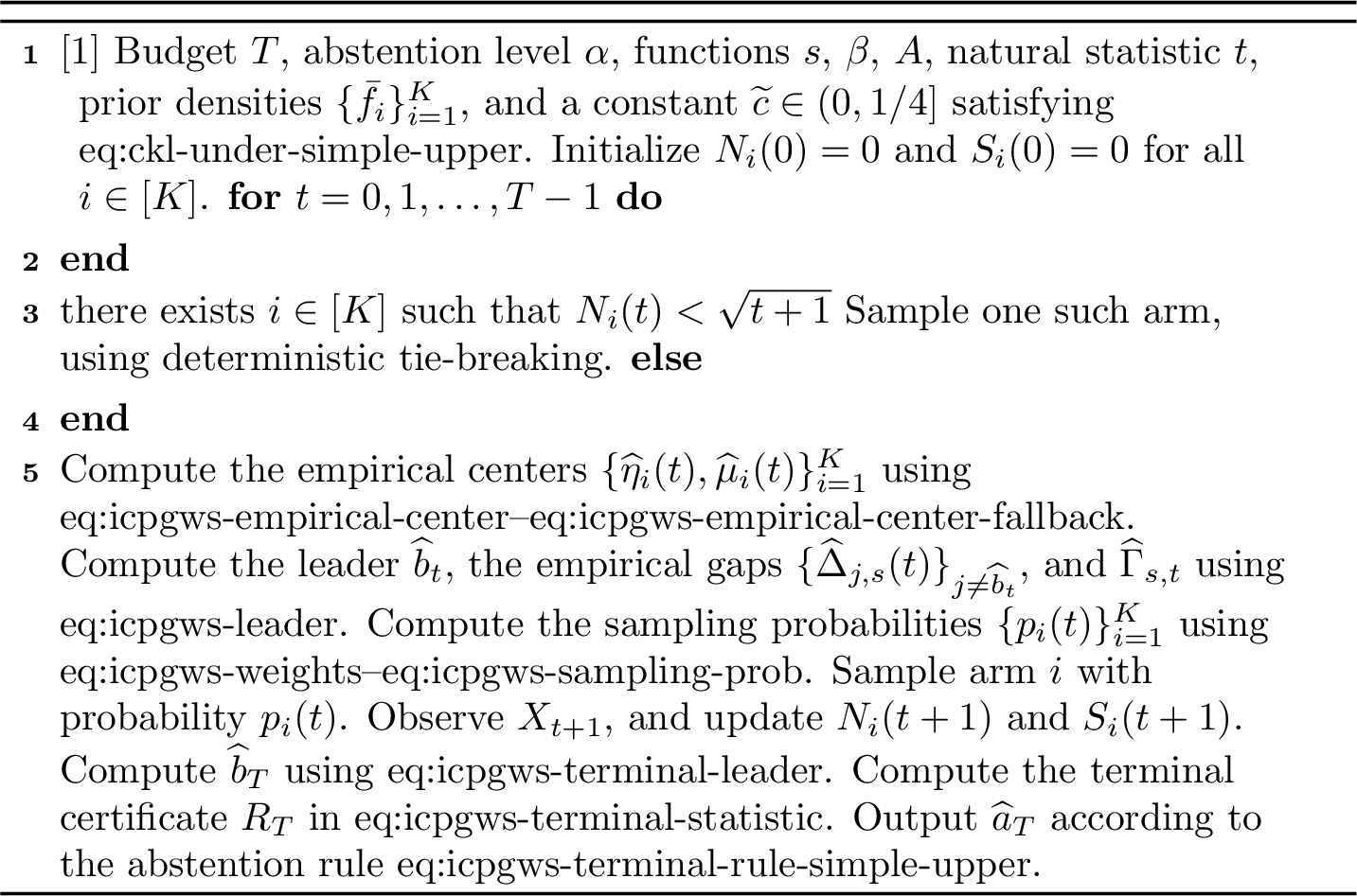
12.3.2 Upper Bound Theorem↩︎
Theorem 7 (Upper Bound for IC-PGWS). Under Assumptions [ass:regular-expfam], [ass:regular-info-prior], and the global quadratic KL assumption [ass:quadratic-kl], \(\mathrm{\small IC-PGWS}(\alpha)\) with terminal rule 54 satisfies, for every \(T\) and every \(\alpha\in(0,1)\), \[\mathcal{A}_T(\mathrm{\small IC-PGWS}(\alpha))=\alpha .\] Moreover, \[\limsup_{\alpha\downarrow0} \limsup_{T\to\infty} \frac{1}{\alpha^2T} \log \mathcal{E}_T(\mathrm{\small IC-PGWS}(\alpha)) \le -\frac{1}{8\kappa^2}.\]
We prove the theorem in several steps. Throughout this proof, all probabilities are under the joint Bayesian law induced by Algorithm 5, unless otherwise stated. Recall that \[\eta_i=s(\mu_i), \qquad \beta(\eta)=\theta(s^{-1}(\eta)), \qquad \mathcal{H}=s(\mathcal{I}).\]
12.3.3 Error Guarantee↩︎
Lemma 33 (Error Guarantee). For every \(T\) and every \(\alpha\in(0,1)\), \[\mathcal{E}_T(\mathrm{\small IC-PGWS}(\alpha)) \le (K-1)e^{-r_{T,\alpha}}.\]
Proof. Condition on the terminal history \(\mathcal{F}_T\). If the algorithm recommends \(\widehat b_T\), then \[\mathbb{P}(a^\star\neq \widehat b_T\mid\mathcal{F}_T) \le \sum_{j\neq \widehat b_T} \varPi_T(\mu_j\ge \mu_{\widehat b_T}).\] By the definition of \(R_T\), \[\max_{j\neq\widehat b_T} \varPi_T(\mu_j\ge \mu_{\widehat b_T}) = e^{-R_T}.\] Therefore \[\mathbb{P}(a^\star\neq \widehat b_T\mid\mathcal{F}_T) \le (K-1)e^{-R_T}.\] On the event that the algorithm does not abstain, the terminal quantile rule implies \(R_T\ge r_{T,\alpha}\). Hence \[\begin{align} \mathcal{E}_T(\mathrm{\small IC-PGWS}(\alpha)) = \mathbb{E}\!\left[ \mathbb{1}\{\widehat a_T\neq ?\} \mathbb{P}(a^\star\neq \widehat b_T\mid\mathcal{F}_T) \right] \le (K-1)e^{-r_{T,\alpha}}. \end{align}\] ◻
12.3.4 Consistency and Allocation Convergence.↩︎
We next identify the almost-sure limit of \(R_T/T\). We first introduce the limiting quantities associated with a realized parameter vector. Let \(b^\star := \operatorname*{arg\,max}_{i\in[K]}\eta_i = \operatorname*{arg\,max}_{i\in[K]}\mu_i\) be the true best arm. For each \(j\neq b^\star\), define the information coordinate gap \(\Delta_{j,s} := \eta_{b^\star}-\eta_j\), and define the true top two information gap \(\Gamma_s := \min_{j\neq b^\star}\Delta_{j,s} = \eta_{(1)}-\eta_{(2)}\), where \(\eta_{(1)}>\eta_{(2)}>\cdots>\eta_{(K)}\) are the ordered information-coordinate qualities.
Define the limiting unnormalized sampling weights by \[\label{eq:simple-limiting-weights} w_{b^\star}^\dagger(\eta):=1, \qquad w_j^\dagger(\eta) := \min\left\{ 1,\, \frac{\Gamma_s^2}{4\widetilde{c}\,\Delta_{j,s}^2} \right\}, \qquad j\neq b^\star.\tag{55}\] Let \[W^\dagger(\eta) := \sum_{\ell=1}^K w_\ell^\dagger(\eta), \qquad p_i^\dagger(\eta) := \frac{w_i^\dagger(\eta)}{W^\dagger(\eta)}.\] Because \(\widetilde{c}\le 1/4\), every second-best arm has limiting weight one. Consequently, \[2\le W^\dagger(\eta)\le K, \qquad p_i^\dagger(\eta)>0 \quad\text{for every }i\in[K].\]
For each challenger \(j\neq b^\star\), define its pairwise error exponent \[C_j^\dagger(\mu) := \inf_{z\in[\mu_j,\mu_{b^\star}]} \left\{ p_{b^\star}^\dagger(\eta)D(\mu_{b^\star},z) + p_j^\dagger(\eta)D(\mu_j,z) \right\}.\] The worst-case pairwise error exponent is \[\label{eq:Cdagger-simple-upper} C^\dagger(\mu) := \min_{j\neq b^\star}C_j^\dagger(\mu).\tag{56}\] Equivalently, \[\label{eq:Cdagger-unnormalized-simple-upper} C^\dagger(\mu) = \frac{1}{W^\dagger(\eta)} \min_{j\neq b^\star} \inf_{z\in[\mu_j,\mu_{b^\star}]} \left\{ D(\mu_{b^\star},z) + w_j^\dagger(\eta)D(\mu_j,z) \right\}.\tag{57}\]
We now show that the empirical centers converge to the true qualities, the empirical sampling proportions converge to \(p^\dagger(\eta)\), and the normalized terminal certificate converges to \(C^\dagger(\mu)\).
Lemma 34 (Information Coordinate Center Consistency). Under Algorithm 5, for every arm \(i\), \[\widehat \eta_i(t)\to \eta_i \qquad\text{and}\qquad \widehat \mu_i(t)\to \mu_i \qquad\text{a.s.}\]
Proof. The forced-exploration rule implies \[N_i(t)\to\infty \qquad\text{a.s. for every }i.\] Conditional on \(\mu_i\), the observations from arm \(i\) are i.i.d. from \(P_{\mu_i}\). Since the log-partition function is finite on an open natural-parameter space, the natural statistic has finite mean under \(P_{\mu_i}\), and \[\mathbb{E}_{\mu_i}[t(X)] = A'(\theta(\mu_i)).\] Therefore, by the strong law of large numbers, \[\widehat{t}_i(t) = \frac{1}{N_i(t)} \sum_{r\le t:A_r=i}t(X_r) \to A'(\theta(\mu_i)) \qquad\text{a.s.}\] Because \(\theta(\mu_i)\in\Theta\) and \(\Theta\) is open, \(A'(\theta(\mu_i))\in A'(\Theta)\). Hence \(\widehat{t}_i(t)\in A'(\Theta)\) eventually almost surely. On this eventual event, \[\widehat\theta_i(t) = (A')^{-1}\!\left(\widehat{t}_i(t)\right) \to \theta(\mu_i),\] since \(A''>0\) implies that \(A'\) is strictly increasing and continuous. Thus \[\widehat \eta_i(t) = \beta^{-1}(\widehat\theta_i(t)) \to \beta^{-1}(\theta(\mu_i)) = s(\mu_i) = \eta_i.\] Continuity of \(s^{-1}\) gives \[\widehat \mu_i(t)=s^{-1}(\widehat \eta_i(t))\to \mu_i.\] ◻
Lemma 35 (Sampling Proportions). Under Algorithm 5, \[\frac{N_i(T)}{T} \to p_i^\dagger(\eta) \qquad\text{a.s. for every }i\in[K].\]
Proof. By Lemma 34, \[\widehat \eta_i(t)\to \eta_i \qquad\text{for every }i.\] Since the prior densities are continuous, ties have probability zero. Thus the best arm and the second-best arm are unique almost surely. On this probability-one event, \(\widehat b_t=b^\star\) eventually, and \[\widehat\Delta_{j,s}(t)\to\Delta_{j,s}, \qquad \widehat\Gamma_{s,t}\to\Gamma_s.\] Therefore \[w_i(t)\to w_i^\dagger(\eta), \qquad p_i(t)\to p_i^\dagger(\eta) \qquad\text{a.s. for every }i.\]
Now fix an arm \(i\). We take four steps:
Step 1: Forced exploration is negligible. Let \(F_i(T)\) be the number of forced-exploration pulls of arm \(i\) up to time \(T\). If the \(m\)-th forced pull of arm \(i\) occurs before time \(T\), then immediately before that pull, \(N_i(t)\ge m-1\). But a forced pull of arm \(i\) can occur only if \(N_i(t)<\sqrt{t+1}\le \sqrt{T+1}\). Hence \(m-1<\sqrt{T+1}\), and therefore \(F_i(T)\le \lceil \sqrt{T+1}\rceil+1\). Consequently, \[\frac{F_i(T)}{T}\to0.\] Let \(F(T)\) be the total number of forced-exploration rounds up to time \(T\). Since \(F(T)=\sum_{\ell=1}^K F_\ell(T)\), we also have \[\frac{F(T)}{T}\le \frac{K(\lceil\sqrt{T+1}\rceil+1)}{T} \to0.\]
Step 2: Martingale concentration on non-forced rounds. Let \(\mathcal{F}_t\) be the history before round \(t+1\), and define \(B_t := \mathbb{1}\{\text{round }t+1\text{ is non-forced}\}\). The event \(\{B_t=1\}\) is \(\mathcal{F}_t\)-measurable. On non-forced rounds, the algorithm samples arm \(i\) with conditional probability \(p_i(t)\).
Define \(D_{i,t+1} := B_t\Bigl(\mathbb{1}\{A_{t+1}=i\}-p_i(t)\Bigr)\). Then \(\mathbb{E}[D_{i,t+1}\mid \mathcal{F}_t]=0\), so \((D_{i,t+1})_{t\ge0}\) is a martingale difference sequence. Also, \(|D_{i,t+1}|\le1\).
Therefore, by Azuma’s inequality, for every \(\varepsilon>0\), \[\mathbb{P}\left( \left| \frac{1}{T}\sum_{t=0}^{T-1}D_{i,t+1} \right| \ge \varepsilon \right) \le 2\exp\left(-\frac{\varepsilon^2T}{2}\right).\] The right-hand side is summable in \(T\). Hence, by the Borel–Cantelli lemma, \[\frac{1}{T}\sum_{t=0}^{T-1}D_{i,t+1}\to0 \qquad\text{almost surely}.\]
Step 3: Decomposition of the empirical pull count. The total number of pulls of arm \(i\) can be decomposed as \[N_i(T) = F_i(T) + \sum_{t=0}^{T-1} B_t\mathbb{1}\{A_{t+1}=i\}.\] Using the definition of \(D_{i,t+1}\), we have \(B_t\mathbb{1}\{A_{t+1}=i\} = D_{i,t+1}+B_t p_i(t)\). Thus \[\frac{N_i(T)}{T} = \frac{F_i(T)}{T} + \frac{1}{T}\sum_{t=0}^{T-1}D_{i,t+1} + \frac{1}{T}\sum_{t=0}^{T-1}B_t p_i(t).\] By Steps 1 and 2, \[\frac{N_i(T)}{T} - \frac{1}{T}\sum_{t=0}^{T-1}B_t p_i(t) \to0 \qquad\text{almost surely}.\]
Step 4: Cesàro convergence of the target probabilities. Since \[p_i(t)\to p_i^\dagger(\eta) \qquad\text{almost surely},\] the sequence \(\{p_i(t)\}\) is Cesàro convergent, i.e., \[\frac{1}{T}\sum_{t=0}^{T-1}p_i(t) \to p_i^\dagger(\eta) \qquad\text{almost surely}.\]
Now write \[\frac{1}{T}\sum_{t=0}^{T-1}B_t p_i(t) = \frac{1}{T}\sum_{t=0}^{T-1}p_i(t) - \frac{1}{T}\sum_{t=0}^{T-1}(1-B_t)p_i(t).\] Since \(0\le p_i(t)\le1\), \[0\le \frac{1}{T}\sum_{t=0}^{T-1}(1-B_t)p_i(t) \le \frac{1}{T}\sum_{t=0}^{T-1}(1-B_t) = \frac{F(T)}{T} \to0.\] Hence \[\frac{1}{T}\sum_{t=0}^{T-1}B_t p_i(t) \to p_i^\dagger(\eta) \qquad\text{almost surely}.\] Combining this with Step 3 gives the desired result. ◻
12.3.5 Posterior Ordering Large Deviations↩︎
Let \(X_{i,1},\ldots,X_{i,n}\) denote the first \(n\) rewards observed from arm \(i\), and let \(\mathcal{G}_{i,n}:=\sigma(X_{i,1},\ldots,X_{i,n})\). Define the one-arm posterior \(\varPi_{i,n}\) as the conditional distribution of \(\eta_i=s(\mu_i)\) given \(\mathcal{G}_{i,n}\): \[\varPi_{i,n}(B) := \mathbb{P}(\eta_i\in B\mid\mathcal{G}_{i,n}), \qquad B\in\mathcal{B}(\mathcal{H}).\] Intuitively, the next lemma proves that \[\varPi_{i,n} (\mu_i'\approx z) = \exp\{ -nD(\mu_i,z) + o(n) \}\]
Lemma 36 (One-arm Posterior Estimates for Ordering). Fix an arm \(i\), and work on the event (that happens almost surely) \[\frac{1}{n}\sum_{r=1}^nt(X_{i,r}) \to A'(\theta(\mu_i)).\] Let \(\varPi_{i,n}\) be the one-arm posterior defined above. Define \[I_i(\eta):=D(\mu_i,s^{-1}(\eta)).\] Then the following hold.
First, for every compact interval \(K\Subset\mathcal{H}\), \[\limsup_{n\to\infty} \frac{1}{n}\log\varPi_{i,n}(K) \le -\inf_{\eta\in K} I_i(\eta).\] Second, for every nonempty open interval \(G\subseteq\mathcal{H}\), \[\liminf_{n\to\infty} \frac{1}{n}\log\varPi_{i,n}(G) \ge -\inf_{\eta\in G} I_i(\eta).\] Third, for every \(a,b\in\mathcal{H}\) with \(a<\eta_i<b\), \[\limsup_{n\to\infty} \frac{1}{n}\log\varPi_{i,n}(\eta\le a) \le -I_i(a),\] and \[\limsup_{n\to\infty} \frac{1}{n}\log\varPi_{i,n}(\eta\ge b) \le -I_i(b).\]
Proof. Set \[\eta_i=s(\mu_i), \qquad \theta_i:=\theta(\mu_i)=\beta(\eta_i), \qquad m_i:=A'(\theta_i),\] and write \[\bar m_n:=\frac{1}{n}\sum_{r=1}^nt(X_{i,r}).\]
For \(\eta\in\mathcal{H}\), write \[p_\eta(w) := \frac{\mathrm{d}P_{s^{-1}(\eta)}}{\mathrm{d}\lambda}(w) = \exp\{\beta(\eta)t(w)-A(\beta(\eta))\}h(w).\] Consider a realized full adaptive history \(h_t=(a_1,x_1,\ldots,a_t,x_t)\), For a candidate parameter vector \(\boldsymbol{\eta}=(\eta_1,\ldots,\eta_K)\in\mathcal{H}^K\), the density of this realized history under the policy \(\pi\), with respect to counting measure on actions and \(\lambda^{\otimes t}\) on rewards, is \[L_t^\pi(\boldsymbol{\eta};h_t) = \prod_{r=1}^t \pi_r(a_r\mid h_{r-1}) \prod_{r=1}^t p_{\eta_{a_r}}(x_r).\] Here \(\pi_r(a_r\mid h_{r-1})\) is the sampling probability assigned by the policy to the realized action \(a_r\) after the realized past \(h_{r-1}\).
Using the product prior in information coordinates, the posterior density of \(\boldsymbol{\eta}\) is therefore proportional to \[\prod_{\ell=1}^K \bar f_\ell(\eta_\ell) \prod_{r:a_r=\ell} p_{\eta_\ell}(x_r).\] Thus the posterior factorizes arm by arm. In particular, the marginal posterior of arm \(i\) depends only on the rewards observed from arm \(i\). If these rewards are denoted \(X_{i,1},\ldots,X_{i,n}\), then, for every measurable set \(B\subseteq\mathcal{H}\), \[\varPi_{i,n}(B) = \frac{ \int_B \bar f_i(\eta) \prod_{r=1}^n p_\eta(X_{i,r}) \,\mathrm{d}\eta }{ \int_{\mathcal{H}} \bar f_i(\eta) \prod_{r=1}^n p_\eta(X_{i,r}) \,\mathrm{d}\eta }.\] Substituting the exponential-family density gives \[\prod_{r=1}^n p_\eta(X_{i,r}) = \exp\left\{ \beta(\eta)\sum_{r=1}^nt(X_{i,r}) - nA(\beta(\eta)) \right\} \prod_{r=1}^n h(X_{i,r}).\] \(\prod_{r=1}^n h(X_{i,r})\) does not depend on \(\eta\), so it also cancels between numerator and denominator. Bayes’ rule gives \[\varPi_{i,n}(B) = \frac{ \int_B \bar f_i(\eta) \exp\{n[\beta(\eta)\bar m_n-A(\beta(\eta))]\} \,\mathrm{d}\eta }{ \int_{\mathcal{H}} \bar f_i(\eta) \exp\{n[\beta(\eta)\bar m_n-A(\beta(\eta))]\} \,\mathrm{d}\eta }.\] Multiplying both numerator and denominator by \[\exp\{-n[\beta(\eta_i)\bar m_n-A(\beta(\eta_i))]\}\] allows us to write \[\varPi_{i,n}(B) = \frac{ \int_B \bar f_i(\eta)e^{nL_n(\eta)}\,\mathrm{d}\eta }{ Z_n },\] where \[L_n(\eta) := (\beta(\eta)-\beta(\eta_i))\bar m_n - A(\beta(\eta)) + A(\beta(\eta_i))\] and \[Z_n := \int_{\mathcal{H}}\bar f_i(\eta)e^{nL_n(\eta)}\,\mathrm{d}\eta.\] Note \(L_n(\eta_i)=0\) and \[L_n(\eta)\to (\beta(\eta)-\beta(\eta_i))A'(\beta(\eta_i)) - A(\beta(\eta))+A(\beta(\eta_i)) = -D(\mu_i,s^{-1}(\eta))=-I_i(\eta)\] on compact subsets of \(\mathcal{H}\).
We first prove that \[\label{eq:one-arm-denominator-rate-simple-upper} \frac{1}{n}\log Z_n\to0.\tag{58}\]
For the lower bound on \(Z_n\), fix \(\tau>0\). Since \(\bar m_n\to m_i\), \(L_n(\eta)\to -I_i(\eta)\) uniformly on compact neighborhoods of \(\eta_i\).
Since \(I_i(\eta_i)=0\), choose a compact interval \(J_\tau\Subset\mathcal{H}\) containing \(\eta_i\) such that, for all sufficiently large \(n\), \(\inf_{\eta\in J_\tau}L_n(\eta)\ge -\tau\).
By continuity and strict positivity of \(\bar f_i\), \[\int_{J_\tau}\bar f_i(\eta)\,\mathrm{d}\eta>0.\] Therefore \[Z_n \ge \int_{J_\tau}\bar f_i(\eta)e^{nL_n(\eta)}\,\mathrm{d}\eta \ge e^{-n\tau}\int_{J_\tau}\bar f_i(\eta)\,\mathrm{d}\eta.\] Thus \[\liminf_{n\to\infty}\frac{1}{n}\log Z_n\ge -\tau.\] Letting \(\tau\downarrow0\) gives \[\liminf_{n\to\infty}\frac{1}{n}\log Z_n\ge0.\]
For the upper bound on \(Z_n\), for all large \(n\) we have \(\bar m_n\in A'(\Theta)\). Define the pseudo-MLE \[\theta_n:=(A')^{-1}(\bar m_n), \qquad \eta_n:=\beta^{-1}(\theta_n).\] Then \(\theta_n\to\theta_i\) and \(\eta_n\to \eta_i\). Moreover, using \(\bar m_n=A'(\theta_n)\), \[\begin{align} L_n(\eta_n)-L_n(\eta) &= (\theta_n-\beta(\eta))A'(\theta_n) - A(\theta_n) + A(\beta(\eta)) \\ &= D(s^{-1}(\eta_n),s^{-1}(\eta)). \end{align}\] Therefore, by assumption 44 , \[L_n(\eta) \le L_n(\eta_n)-\widetilde{c}\,(\eta-\eta_n)^2.\] Since \[L_n(\eta_n) = D(s^{-1}(\eta_n),\mu_i) \to0,\] boundedness of \(\bar f_i\) gives \[\begin{align} Z_n &\le \|\bar f_i\|_\infty e^{nL_n(\eta_n)} \int_{\mathcal{H}}e^{-n\widetilde{c} (\eta-\eta_n)^2}\,\mathrm{d}\eta \\ &\le \|\bar f_i\|_\infty e^{nL_n(\eta_n)} \sqrt{\frac{\pi}{n\widetilde{c}}}. \end{align}\] Hence \[\limsup_{n\to\infty}\frac{1}{n}\log Z_n\le0.\] This proves 58 .
Now fix a compact interval \(K\Subset\mathcal{H}\). Since \(\bar m_n\to m_i\), \[L_n(\eta)\to -D(\mu_i,s^{-1}(\eta))=-I_i(\eta)\] uniformly on \(K\). Hence \[\begin{align} \limsup_{n\to\infty} \frac{1}{n}\log \int_K \bar f_i(\eta)e^{nL_n(\eta)}\,\mathrm{d}\eta &\le -\inf_{\eta\in K}I_i(\eta). \end{align}\] Combining this numerator bound with 58 gives the compact-interval upper bound.
Next let \(G\subseteq\mathcal{H}\) be a nonempty open interval. Choose \(\eta_0\in G\) such that \[I_i(\eta_0)\le \inf_{\eta\in G}I_i(\eta)+\tau.\] Choose a compact interval \(J\Subset G\) containing \(\eta_0\) and small enough that \[\sup_{\eta\in J}I_i(\eta)\le I_i(\eta_0)+\tau.\] By uniform convergence of \(L_n\) on \(J\) and strict positivity of \(\bar f_i\) on \(J\), \[\begin{align} \liminf_{n\to\infty} \frac{1}{n}\log \int_G \bar f_i(\eta)e^{nL_n(\eta)}\,\mathrm{d}\eta &\ge \liminf_{n\to\infty} \frac{1}{n}\log \int_J \bar f_i(\eta)e^{nL_n(\eta)}\,\mathrm{d}\eta \\ &\ge -\sup_{\eta\in J}I_i(\eta) \ge -\inf_{\eta\in G}I_i(\eta)-2\tau. \end{align}\] Using again the denominator rate 58 , and then letting \(\tau\downarrow0\), gives the open-interval lower bound.
It remains to prove the one-sided estimates. Consider \(a<\eta_i\). Since \(\eta_n\to \eta_i\), eventually \(a<\eta_n\). The function \(\theta\mapsto \theta\bar m_n-A(\theta)\) is strictly concave and maximized at \(\theta_n\). Since \(\beta\) is strictly increasing, \(L_n(\eta)\) is increasing on \(\{\eta<\eta_n\}\). Therefore, for all large \(n\), \[\sup_{\eta\le a}L_n(\eta)=L_n(a).\] Thus \[\varPi_{i,n}(\eta\le a) \le \frac{e^{nL_n(a)}}{Z_n},\] because \(\int_{\{\eta\le a\}}\bar f_i(\eta)\,\mathrm{d}\eta\le1\). Since \(L_n(a)\to -I_i(a)\) and \(n^{-1}\log Z_n\to0\), we obtain \[\limsup_{n\to\infty} \frac{1}{n}\log\varPi_{i,n}(\eta\le a) \le -I_i(a).\] The proof for \(b>\eta_i\) is identical: eventually \(b>\eta_n\), \(L_n\) is decreasing on \(\{\eta>\eta_n\}\), and hence \[\sup_{\eta\ge b}L_n(\eta)=L_n(b).\] This gives the upper-tail estimate. ◻
The following lemma shows that, if arms \(i\) and \(j\) receive asymptotic sampling proportions \(q_i\) and \(q_j\), then the posterior probability of incorrectly ordering them decays with exponent \[\inf_{z\in[\mu_j,\mu_i]} \{q_iD(\mu_i,z)+q_jD(\mu_j,z)\}.\]
Lemma 37 (Posterior Ordering Large Deviations). Fix two arms \(i\) and \(j\) with \(\mu_i>\mu_j\). Suppose that \[\frac{N_i(T)}{T}\to q_i>0, \qquad \frac{N_j(T)}{T}\to q_j>0.\] Then almost surely \[\label{eq:behavior95of95Pi} -\frac{1}{T} \log \varPi_T(\mu_j\ge \mu_i) \to \inf_{z\in[\mu_j,\mu_i]} \{q_iD(\mu_i,z)+q_jD(\mu_j,z)\}.\qquad{(29)}\]
Proof. Write \[\eta_i=s(\mu_i), \qquad \eta_j=s(\mu_j), \qquad \eta_i>\eta_j.\] Recall from the proof of Lemma 36 that, conditional on the realized history, the arm-wise posterior of \(\eta_i=s(\mu_i)\) is \[\varPi_{i,T}(\mathrm{d}\eta) = \frac{ \bar f_i(\eta) \exp\{\beta(\eta)S_i(T)-N_i(T)A(\beta(\eta))\} }{ Z_{i,T} }\,\mathrm{d}\eta,\] where \[Z_{i,T} := \int_{\mathcal{H}} \bar f_i(u) \exp\{\beta(u)S_i(T)-N_i(T)A(\beta(u))\} \,\mathrm{d}u .\] Because the prior is a product prior and the likelihood factors arm by arm, the full posterior factorizes: \[\varPi_T(\mathrm{d}\eta_1,\ldots,\mathrm{d}\eta_K) = \bigotimes_{\ell=1}^K \varPi_{\ell,T}(\mathrm{d}\eta_\ell).\] Consequently, let \(U\sim\varPi_{i,T}\) and \(V\sim\varPi_{j,T}\) denote the posterior information coordinate qualities (arm parameter) of arms \(i\) and \(j\), then \(U\) and \(V\) are independent under the posterior, and for Borel sets \(B,C\subseteq\mathcal{H}\), \[\varPi_T(U\in B,\;V\in C) = \varPi_{i,T}(B)\varPi_{j,T}(C).\] In particular, \[\varPi_T(\mu_j\ge \mu_i) = \varPi_T(\eta_j\ge \eta_i) = \varPi_T(V\ge U).\] Define \[I_i(u):=D(\mu_i,s^{-1}(u)), \qquad I_j(v):=D(\mu_j,s^{-1}(v)),\] and \[C_{ij} := \inf_{w\in[\eta_j,\eta_i]} \{q_iI_i(w)+q_jI_j(w)\}.\] The one-arm bounds on \(\log \varPi_{i,n}\) of Lemma 36 hold along every subsequence \(n\to\infty\) on the arm-wise strong-law event. Therefore they also hold along the random subsequences \(N_i(T)\) and \(N_j(T)\). Multiplying the one-arm exponents by \(N_i(T)/T\to q_i\) and \(N_j(T)/T\to q_j\) gives the corresponding \(T\)-speed bounds: For intervals \(B,C\), \[\limsup_{T\to\infty} \frac{1}{T}\log\{\varPi_{i,T}(B)\varPi_{j,T}(C)\} \le -q_i\inf_{u\in B}I_i(u)-q_j\inf_{v\in C}I_j(v)\] when \(B,C\) are compact, and the corresponding lower bound when \(B,C\) are open.
We first prove the lower bound for ?? . Let \(w^\star\in[\eta_j,\eta_i]\) be a minimizer of \[w\mapsto q_iI_i(w)+q_jI_j(w).\] If \(w^\star\in(\eta_j,\eta_i)\), choose \(\delta>0\) so small that \[(w^\star-\delta,w^\star) \times (w^\star,w^\star+\delta) \subseteq \{(u,v):v\ge u\}.\] Then, by posterior product decomposition and the open-interval lower bounds in Lemma 36, \[\begin{align} \liminf_{T\to\infty} \frac{1}{T}\log \varPi_T(V\ge U) &\ge -q_i\inf_{u\in(w^\star-\delta,w^\star)}I_i(u) -q_j\inf_{v\in(w^\star,w^\star+\delta)}I_j(v). \end{align}\] Letting \(\delta\downarrow0\) gives \[\liminf_{T\to\infty} \frac{1}{T}\log \varPi_T(V\ge U) \ge -C_{ij}.\] If \(w^\star=\eta_j\), use instead the rectangle \(U\in(\eta_j-\delta,\eta_j)\) and \(V\in(\eta_j,\eta_j+\delta)\). Since \[\inf_{u\in(\eta_j-\delta,\eta_j)} I_i(u)\to I_i(\eta_j), \qquad \inf_{v\in(\eta_j,\eta_j+\delta)} I_j(v)\to I_j(\eta_j)=0,\] the same lower bound follows.
Similarly if \(w^\star=\eta_i\), use \(U\in(\eta_i-\delta,\eta_i)\) and \(V\in(\eta_i,\eta_i+\delta)\). Then \[\inf_{u\in(\eta_i-\delta,\eta_i)} I_i(u)\to I_i(\eta_i)=0, \qquad \inf_{v\in(\eta_i,\eta_i+\delta)} I_j(v)\to I_j(\eta_i),\] and the same lower bound again follows. Thus \[\liminf_{T\to\infty} \frac{1}{T}\log \varPi_T(V\ge U) \ge -C_{ij}.\]
For the upper bound, decompose \[\{V\ge U\} \subseteq E_-\cup E_0\cup E_+,\] where \(E_-:=\{U\le \eta_j\}\), \(E_+:=\{V\ge \eta_i\}\) and \(E_0:=\{\eta_j\le U\le V\le \eta_i\}\).
The one-sided estimates in Lemma 36 give \[\limsup_{T\to\infty} \frac{1}{T}\log\varPi_T(E_-) \le -q_i I_i(\eta_j) = -q_iD(\mu_i,\mu_j),\] and \[\limsup_{T\to\infty} \frac{1}{T}\log\varPi_T(E_+) \le -q_j I_j(\eta_i) = -q_jD(\mu_j,\mu_i).\] Since \(C_{ij}\le q_iD(\mu_i,\mu_j)\), by taking \(w=\eta_j\), and \(C_{ij}\le q_jD(\mu_j,\mu_i)\), by taking \(w=\eta_i\), both endpoint events have exponent at least \(C_{ij}\).
It remains to control \(E_0\). The set \(K_0:=\{(u,v):\eta_j\le u\le v\le \eta_i\}\) is compact. Fix \(\tau>0\). By continuity of \((u,v)\mapsto q_iI_i(u)+q_jI_j(v)\) on the compact square \([\eta_j,\eta_i]^2\), there exist finitely many compact rectangles \[R_m=I_m\times J_m,\qquad m=1,\ldots,M,\] whose union covers \(K_0\), such that each \(R_m\subseteq[\eta_j,\eta_i]^2\) and \[\inf_{(u,v)\in R_m} \{q_iI_i(u)+q_jI_j(v)\} \ge \inf_{(u,v)\in K_0} \{q_iI_i(u)+q_jI_j(v)\} -\tau .\] By posterior product decomposition, \[\varPi_T(E_0) \le \sum_{m=1}^M \varPi_{i,T}(I_m)\varPi_{j,T}(J_m),\] where \(\varPi_{i,T}\) and \(\varPi_{j,T}\) are the corresponding arm-wise posterior marginals. Applying the compact-interval upper bound from Lemma 36 along the subsequences \(N_i(T)\) and \(N_j(T)\), we get, for each \(m\), \[\begin{align} \limsup_{T\to\infty} \frac{1}{T}\log\{\varPi_{i,T}(I_m)\varPi_{j,T}(J_m)\} &\le -q_i\inf_{u\in I_m}I_i(u) -q_j\inf_{v\in J_m}I_j(v) \\ &= -\inf_{(u,v)\in R_m} \{q_iI_i(u)+q_jI_j(v)\}. \end{align}\] Since the cover is finite, the union bound yields \[\begin{align} \limsup_{T\to\infty} \frac{1}{T}\log\varPi_T(E_0) &\le - \inf_{(u,v)\in K_0} \{q_iI_i(u)+q_jI_j(v)\} +\tau . \end{align}\] Letting \(\tau\downarrow0\), we obtain \[\limsup_{T\to\infty} \frac{1}{T}\log\varPi_T(E_0) \le - \inf_{\eta_j\le u\le v\le \eta_i} \{q_iI_i(u)+q_jI_j(v)\}.\]
We now reduce this infimum to the diagonal (\(u=v\)). Note the derivative \[\frac{\partial }{\partial z} D(\mu,z) = \theta'(z)\left[ A'(\theta(z))-A'(\theta(\mu)) \right],\] is negative for \(z<\mu\) and positive for \(z>\mu\). Hence, on the interval \([\eta_j,\eta_i]\), the map \(u\mapsto I_i(u)\) is non-increasing whereas \(v\mapsto I_j(v)\) is non-decreasing. Therefore, if \(u\le v\), then for every \(w\in[u,v]\), \(I_i(w)\le I_i(u)\) and \(I_j(w)\le I_j(v)\).
Thus every feasible off-diagonal point can be moved to a diagonal point with no larger objective. Hence \[\inf_{\eta_j\le u\le v\le \eta_i} \{q_iI_i(u)+q_jI_j(v)\} = \inf_{w\in[\eta_j,\eta_i]} \{q_iI_i(w)+q_jI_j(w)\} = C_{ij}.\] Combining the bounds for \(E_-\), \(E_0\), and \(E_+\) by a union bound gives \[\limsup_{T\to\infty} \frac{1}{T}\log \varPi_T(V\ge U) \le -C_{ij}.\] Together with the lower bound, \[-\frac{1}{T}\log\varPi_T(V\ge U)\to C_{ij}.\] Returning to \(z=s^{-1}(w)\) proves the claimed formula. ◻
12.3.6 Asymptotic Behavior of the Certificate \(R_T\)↩︎
Recall we defined \[C^\dagger(\mu) := \min_{j\neq b^\star} \inf_{z\in[\mu_j,\mu_{b^\star}]} \left\{ p_{b^\star}^\dagger(\eta) D(\mu_{b^\star},z) + p_j^\dagger(\eta) D(\mu_j,z) \right\}.\]
Lemma 38 (Terminal Certificate Limit). Under Algorithm 5, \[\frac{R_T}{T} \to C^\dagger(\mu) \qquad\text{a.s.}\]
Proof. By Lemma 34, \(\widehat b_T=b^\star\) eventually almost surely. By Lemma 35, \[\frac{N_i(T)}{T}\to p_i^\dagger(\eta) \qquad\text{for every }i.\] Since \(p_i^\dagger(\eta)>0\) for every arm, applying Lemma 37 with \(i=b^\star\) and each \(j\neq b^\star\) gives \[-\frac{1}{T} \log \varPi_T(\mu_j\ge \mu_{b^\star}) \to \inf_{z\in[\mu_j,\mu_{b^\star}]} \left\{ p_{b^\star}^\dagger(\eta) D(\mu_{b^\star},z) + p_j^\dagger(\eta) D(\mu_j,z) \right\}.\] Taking the minimum over the finite set \(j\neq b^\star\) yields \[\frac{R_T}{T} = \min_{j\neq b^\star} \left\{ -\frac{1}{T}\log \varPi_T(\mu_j\ge \mu_{b^\star}) \right\} \to C^\dagger(\mu).\] ◻
12.3.7 Lower Tail of the Limiting Certificate.↩︎
We now prove that \(C^\dagger(\mu)\) has the same small lower tail as \(\Gamma_s^2/8\).
Lemma 39 (Top-Two Gap and Triple-Gap Expansions). Under Assumption [ass:regular-info-prior], \[\mathbb{P}(\Gamma_s\le\varepsilon) = \kappa\varepsilon+o(\varepsilon), \qquad \varepsilon\downarrow0.\] Moreover, define \(\Gamma_{3,s}:=\eta_{(1)}-\eta_{(3)}\) for \(K\ge3\), and \(\Gamma_{3,s}:=+\infty\) for \(K=2\), then \[\mathbb{P}(\Gamma_{3,s}\le\varepsilon) = O(\varepsilon^2).\]
Proof. For the top-two gap expansion, condition on arm \(i\) having information coordinate value \(u\). The event that arm \(i\) is best and that the top-two gap is at most \(\varepsilon\) has conditional probability \[\prod_{k\neq i}\bar F_k(u) - \prod_{k\neq i}\bar F_k(u-\varepsilon),\] where \(\bar F_k(t)\) is understood to be \(0\) below the left endpoint of \(\mathcal{H}\) and \(1\) above the right endpoint. Hence \[\mathbb{P}(\Gamma_s\le\varepsilon) = \sum_{i=1}^K \int_{\mathcal{H}} \bar f_i(u) \left[ \prod_{k\neq i}\bar F_k(u) - \prod_{k\neq i}\bar F_k(u-\varepsilon) \right]\mathrm{d}u.\] Let \[G_i(u):=\prod_{k\neq i}\bar F_k(u).\] Then \[G_i'(u) = \sum_{j\neq i} \bar f_j(u)\prod_{k\neq i,j}\bar F_k(u)\] where the derivative exists, and \(G_i\) is Lipschitz because the densities are bounded. Therefore \[\frac{G_i(u)-G_i(u-\varepsilon)}{\varepsilon} \to G_i'(u)\] for almost every \(u\), and the quotient is uniformly bounded. Dominated convergence gives \[\begin{align} \frac{\mathbb{P}(\Gamma_s\le\varepsilon)}{\varepsilon} \to \sum_{i=1}^K \sum_{j\neq i} \int_{\mathcal{H}} \bar f_i(u)\bar f_j(u) \prod_{k\neq i,j}\bar F_k(u)\,\mathrm{d}u =\kappa . \end{align}\]
For the triple-gap bound, the case \(K=2\) is trivial. Assume \(K\ge3\), and let \[M_{\bar{f}}:=\max_{i\in[K]}\|\bar f_i\|_\infty<\infty.\] If \(\Gamma_{3,s}\le\varepsilon\), then there exist three distinct arms \(i,j,k\) whose information coordinate values all lie in an interval of length \(\varepsilon\) below the largest of the three. Hence, by a union bound over ordered triples, \[\begin{align} \mathbb{P}(\Gamma_{3,s}\le\varepsilon) &\le \sum_{i,j,k\;{\rm distinct}} \int_{\mathcal{H}} \bar f_i(u) \left[ \int_{u-\varepsilon}^{u}\bar f_j(v)\,\mathrm{d}v \right] \left[ \int_{u-\varepsilon}^{u}\bar f_k(w)\,\mathrm{d}w \right]\mathrm{d}u \\ &\le K(K-1)(K-2)M_{\bar{f}}^2\varepsilon^2. \end{align}\] ◻
Define the ordered top-pair tie manifold \[\mathcal{T}^\uparrow := \biguplus_{i\neq j} \left\{ (i,j,u,\zeta_{-ij}): u\in\mathcal{H},\;\zeta_k\in\mathcal{H},\;\zeta_k<u\;\forall k\neq i,j \right\}.\] Here \(i\) denotes the best arm and \(j\) denotes the second-best arm. For a parameter vector \(\eta\) with unique best and second-best arms, define \[\xi^\uparrow(\eta) := \bigl(b^\star,b^\star_2,\eta_{b^\star},(\eta_k)_{k\neq b^\star,b^\star_2}\bigr),\] where \(b^\star\) is the best arm index, and \(b^\star_2\) is the second-best arm index. Note that it does not include \(\eta_{b^\star_2}\), which is meant to be recovered by \(\Gamma_s\).
On the component \((i,j)\), define the finite measure \[\lambda(\mathrm{d}\xi) := \bar f_i(u)\bar f_j(u) \prod_{k\neq i,j}\bar f_k(\zeta_k)\,\mathrm{d}u\,\mathrm{d}\zeta_{-ij}.\] Then \(\lambda(\mathcal{T}^\uparrow)=\kappa\).
Lemma 40 (Compact Localization of Top-Two Gap Density). For every \(\rho>0\), there exists a compact set \[\mathcal{K}_\rho\subset\mathcal{T}^\uparrow\] such that, for every fixed \(R<\infty\), \[\mathbb{P}\{\Gamma_s\le R\varepsilon,\, \xi^\uparrow(\eta)\in\mathcal{K}_\rho\} \ge (\kappa-\rho)R\varepsilon+o(\varepsilon),\] and \[\mathbb{P}\{\Gamma_s\le R\varepsilon,\, \xi^\uparrow(\eta)\notin\mathcal{K}_\rho\} \le \rho R\varepsilon+o(\varepsilon),\] as \(\varepsilon\downarrow0\).
Proof. Since \(\mathcal{T}^\uparrow\) is a finite disjoint union of open subsets of Euclidean spaces and \(\lambda\) is a finite Borel measure with density with respect to Lebesgue measure on each component, \(\lambda\) is a finite Radon measure. In particular, it is inner regular. Choose a compact set \(\mathcal{K}_\rho\subset\mathcal{T}^\uparrow\) such that \(\lambda(\mathcal{K}_\rho)\ge \kappa-\rho\).
Because \(\mathcal{K}_\rho\) is compact and lies inside the open ordered tie manifold, there exists \(\ell_\rho>0\) such that, for every \((i,j,u,\zeta_{-ij})\in\mathcal{K}_\rho\), \(\zeta_k\le u-\ell_\rho\) for all \(k\neq i,j\).
For all sufficiently small \(\varepsilon\), uniformly over \(0\le r\le R\varepsilon\), the second-arm value \(u-r\) remains above all background values on \(\mathcal{K}_\rho\). Hence, restricted to \(\mathcal{K}_\rho\), \[\begin{align} &\mathbb{P}\{\Gamma_s\le R\varepsilon,\, \xi^\uparrow(\eta)\in\mathcal{K}_\rho\} \\ &\quad= \sum_{i\neq j} \int \mathbb{1}_{\{(i,j,u,\zeta_{-ij})\in\mathcal{K}_\rho\}} \bar f_i(u) \prod_{k\neq i,j}\bar f_k(\zeta_k) \left[ \int_{u-R\varepsilon}^{u}\bar f_j(v)\,\mathrm{d}v \right] \mathrm{d}u\,\mathrm{d}\zeta_{-ij}. \end{align}\] By continuity of \(\bar f_j\) on the compact projection of \(\mathcal{K}_\rho\), \[\int_{u-R\varepsilon}^{u}\bar f_j(v)\,\mathrm{d}v = R\varepsilon\,\bar f_j(u)+o(\varepsilon)\] uniformly over \(\mathcal{K}_\rho\). Therefore \[\mathbb{P}\{\Gamma_s\le R\varepsilon,\, \xi^\uparrow(\eta)\in\mathcal{K}_\rho\} = R\varepsilon\,\lambda(\mathcal{K}_\rho)+o(\varepsilon) \ge (\kappa-\rho)R\varepsilon+o(\varepsilon).\] The complement bound follows by subtracting this lower bound from the total top-two gap expansion: \[\mathbb{P}(\Gamma_s\le R\varepsilon) = \kappa R\varepsilon+o(\varepsilon).\] ◻
Lemma 41 (Small Certificate Implies Small Information Gap). There exists a constant \(R^\star<\infty\), depending only on \(K\) and \(\widetilde{c}\), such that \[C^\dagger(\mu)\le u \quad\Longrightarrow\quad \Gamma_s\le R^\star\sqrt u.\]
Proof. Fix \(j\neq b^\star\), write \(\Delta:=\Delta_{j,s}=\eta_{b^\star}-\eta_j\), and \(a:=w_j^\dagger(\eta)\). For \(z\in[\mu_j,\mu_{b^\star}]\), write \(r:=s(z)-\eta_j\in[0,\Delta]\). By 44 , \[\begin{align} D(\mu_{b^\star},z)+aD(\mu_j,z) &\ge \widetilde{c}\{(\Delta-r)^2+a r^2\}. \end{align}\] If \(a=1\), then \[\inf_{0\le r\le\Delta} \widetilde{c}\{(\Delta-r)^2+r^2\} = \frac{\widetilde{c}}{2}\Delta^2 \ge \frac{\widetilde{c}}{2}\Gamma_s^2.\] If \(a<1\), then by 55 , \(a=\frac{\Gamma_s^2}{4\widetilde{c}\,\Delta^2}\). Thus \[\begin{align} \inf_{0\le r\le\Delta} \widetilde{c}\{(\Delta-r)^2+a r^2\} = \widetilde{c}\frac{a}{1+a}\Delta^2 \ge \frac{\widetilde{c} a}{2}\Delta^2 = \frac{\Gamma_s^2}{8}, \end{align}\] where we used \(a<1\). Therefore, for every challenger \(j\), \[\inf_{z\in[\mu_j,\mu_{b^\star}]} \{D(\mu_{b^\star},z)+w_j^\dagger(\eta) D(\mu_j,z)\} \ge c_{\rm gap}\Gamma_s^2,\] where \(c_{\rm gap}:= \min\left\{\frac{\widetilde{c}}{2},\frac{1}{8}\right\}>0\).
Since \(W^\dagger(\eta)\le K\), 57 gives \(C^\dagger(\mu) \ge \frac{c_{\rm gap}}{K}\Gamma_s^2\). Hence \(C^\dagger(\mu)\le u\) implies \[\Gamma_s\le \sqrt{\frac{K}{c_{\rm gap}}}\sqrt u.\] Taking \(R^\star:=\sqrt{K/c_{\rm gap}}\) gives the desired result. ◻
Lemma 42 (Local Expansion of the Limiting Certificate). Fix a compact set \(\mathcal{K}\subset\mathcal{T}^\uparrow\). Uniformly over parameter vectors satisfying \(\xi^\uparrow(\eta)\in\mathcal{K}\) and \(\Gamma_s\downarrow0\), we have \[C^\dagger(\mu) = \frac{\Gamma_s^2}{8}\{1+o(1)\}.\]
Proof. Let \(b^\star_2\) denote the second-best arm and put \(\gamma:=\Gamma_s\).
Because \(\mathcal{K}\) is compactly contained in \(\mathcal{T}^\uparrow\), there exists \(\ell>0\) such that, whenever \(\xi^\uparrow(\eta)\in\mathcal{K}\), \[\eta_{b^\star}-\eta_k\ge \ell, \qquad k\notin\{b^\star,b^\star_2\},\] for all sufficiently small \(\gamma\). Also, all relevant information coordinate values remain in a compact subset of \(\mathcal{H}\).
The KL divergence has the uniform local Fisher coordinate expansion \[\label{eq:local-kl-simple-upper} D(s^{-1}(\eta),s^{-1}(v)) = \frac{1}{2}(\eta-v)^2+O(|\eta-v|^3),\tag{59}\] for \(\eta,v\) in any compact subset of \(\mathcal{H}\). This follows from a Taylor expansion of the KL divergence and the definition of \(s\).
For the top two arms, \(w_{b^\star}^\dagger(\eta)=1\) and \(w_{b^\star_2}^\dagger(\eta) = \min\left\{ 1,\frac{\gamma^2}{4\widetilde{c}\,\gamma^2} \right\} = 1,\) Hence using 59 , \[\begin{align} &\inf_{z\in[\mu_{b^\star_2},\mu_{b^\star}]} \{D(\mu_{b^\star},z)+D(\mu_{b^\star_2},z)\} \\ &\qquad= \inf_{w\in[\eta_{b^\star}-\gamma,\eta_{b^\star}]} \left\{ \frac{1}{2}(\eta_{b^\star}-w)^2 + \frac{1}{2}(w-\eta_{b^\star}+\gamma)^2 \right\} + o(\gamma^2) \\ &\qquad= \frac{\gamma^2}{4}+o(\gamma^2). \end{align}\]
For any other challenger \(k\notin\{b^\star,b^\star_2\}\), its information gap \(\Delta_{k,s}:=\eta_{b^\star}-\eta_k\) is bounded below by \(\ell\). Therefore \(w_k^\dagger(\eta) = \frac{\gamma^2}{4\widetilde{c}\,\Delta_{k,s}^2} = O(\gamma^2)\), for all sufficiently small \(\gamma\). Hence \[W^\dagger(\eta) = 1+w_{b^\star_2}^\dagger(\eta)+\sum_{k\notin\{b^\star,b^\star_2\}}w_k^\dagger(\eta) = 2+O(\gamma^2).\] Furthermore, by the same coercivity calculation as in Lemma 41, \[\begin{align} \inf_{z\in[\mu_k,\mu_{b^\star}]} \{D(\mu_{b^\star},z)+w_k^\dagger(\eta) D(\mu_k,z)\} \ge \widetilde{c} \frac{w_k^\dagger(\eta)}{1+w_k^\dagger(\eta)} \Delta_{k,s}^2 = \frac{\gamma^2}{4}\{1+o(1)\}. \end{align}\] Thus \[\min_{j\neq b^\star} \inf_{z\in[\mu_j,\mu_{b^\star}]} \{D(\mu_{b^\star},z)+w_j^\dagger(\eta) D(\mu_j,z)\} = \frac{\gamma^2}{4}\{1+o(1)\}.\] Combining this with \(W^\dagger(\eta)=2+o(1)\) in 57 gives \[C^\dagger(\mu) = \frac{\gamma^2}{8}\{1+o(1)\}.\] The preceding estimates are uniform on \(\mathcal{K}\), so the proof is complete. ◻
Lemma 43 (Small Lower Tail of the Limiting Certificate). As \(u\downarrow0\), \[\mathbb{P}(C^\dagger(\mu)\le u) = \kappa\sqrt{8u}+o(\sqrt u).\]
Proof. We prove matching lower and upper bounds.
For the lower bound, fix \(\rho>0\) and \(\tau\in(0,1)\). Choose \(\mathcal{K}_\rho\) as in Lemma 40. By the uniform local expansion in Lemma 42, for all sufficiently small \(u\), \[\left\{ \Gamma_s\le (1-\tau)\sqrt{8u}, \;\xi^\uparrow(\eta)\in\mathcal{K}_\rho \right\} \subseteq \{C^\dagger(\mu)\le u\}.\] Indeed, on \(\mathcal{K}_\rho\), \[C^\dagger(\mu) = \frac{\Gamma_s^2}{8}\{1+o(1)\},\] uniformly as \(\Gamma_s\downarrow0\), and the factor \((1-\tau)^2\) leaves enough slack. Therefore, using Lemma 40 with \(\varepsilon=\sqrt u\) and \(R=(1-\tau)\sqrt8\), \[\begin{align} \mathbb{P}(C^\dagger(\mu)\le u) &\ge \mathbb{P}\left( \Gamma_s\le (1-\tau)\sqrt{8u}, \;\xi^\uparrow(\eta)\in\mathcal{K}_\rho \right) \\ &\ge (\kappa-\rho)(1-\tau)\sqrt{8u} + o(\sqrt u). \end{align}\] Letting \(\rho\downarrow0\) and then \(\tau\downarrow0\) yields \[\liminf_{u\downarrow0} \frac{\mathbb{P}(C^\dagger(\mu)\le u)}{\sqrt u} \ge \kappa\sqrt8.\]
For the upper bound, Lemma 41 gives \[\{C^\dagger(\mu)\le u\} \subseteq \{\Gamma_s\le R^\star\sqrt u\}.\] Fix \(\rho>0\), and again use the compact set \(\mathcal{K}_\rho\). On \[\{C^\dagger(\mu)\le u,\;\xi^\uparrow(\eta)\in\mathcal{K}_\rho\},\] Lemma 41 implies \(\Gamma_s\to0\) uniformly as \(u\downarrow0\). Hence the uniform local expansion gives, for all sufficiently small \(u\), \[C^\dagger(\mu) \ge (1-\tau)\frac{\Gamma_s^2}{8}.\] Consequently, on the same event, \[\Gamma_s \le \sqrt{\frac{8u}{1-\tau}} \le (1+\tau)\sqrt{8u},\] after decreasing \(u\) if necessary and replacing \(\tau\) by a smaller slack constant. Therefore \[\begin{align} \mathbb{P}(C^\dagger(\mu)\le u) \le \mathbb{P}\{\Gamma_s\le (1+\tau)\sqrt{8u}\} + \mathbb{P}\{\Gamma_s\le R^\star\sqrt u,\, \xi^\uparrow(\eta)\notin\mathcal{K}_\rho\}. \end{align}\] By Lemmas 39 and 40, \[\mathbb{P}(C^\dagger(\mu)\le u) \le \kappa(1+\tau)\sqrt{8u} + \rho R^\star\sqrt u + o(\sqrt u).\] Letting \(u\downarrow0\), then \(\rho\downarrow0\), and finally \(\tau\downarrow0\), gives \[\limsup_{u\downarrow0} \frac{\mathbb{P}(C^\dagger(\mu)\le u)}{\sqrt u} \le \kappa\sqrt8.\] Combining the two bounds proves the claim. ◻
12.3.8 Lower Bound on the Calibration Threshold↩︎
Lemma 44 (Lower Bound on the Calibration Threshold). For every \(\varepsilon\in(0,1)\), there exists \(\alpha_0>0\) such that, for every \(0<\alpha\le\alpha_0\), there exists \(T_0(\alpha,\varepsilon)<\infty\) such that, for all \(T\ge T_0(\alpha,\varepsilon)\), \[r_{T,\alpha} \ge (1-\varepsilon)\frac{\alpha^2T}{8\kappa^2}.\]
Proof. Set \(c:=\frac{1}{8\kappa^2}\) and \(u_{\alpha,\varepsilon}:=(1-\varepsilon)c\alpha^2\). By Lemma 43, \[\begin{align} \mathbb{P}(C^\dagger(\mu)\le u_{\alpha,\varepsilon}) &= \kappa\sqrt{8(1-\varepsilon)c}\,\alpha+o(\alpha) \\ &= \sqrt{1-\varepsilon}\,\alpha+o(\alpha). \end{align}\] Therefore, for all sufficiently small \(\alpha\), \(\mathbb{P}(C^\dagger(\mu)\le u_{\alpha,\varepsilon})<\alpha\). By Lemma 38, \[\frac{R_T}{T}\to C^\dagger(\mu) \qquad\text{a.s.}\] Thus \(R_T/T\) converges to \(C^\dagger(\mu)\) in distribution. Applying the Portmanteau theorem to the closed set \((-\infty,u_{\alpha,\varepsilon}]\) gives \[\limsup_{T\to\infty} \mathbb{P}\left( \frac{R_T}{T}\le u_{\alpha,\varepsilon} \right) \le \mathbb{P}(C^\dagger(\mu)\le u_{\alpha,\varepsilon}) < \alpha.\] Hence, for all sufficiently large \(T\), \(\mathbb{P}(R_T\le u_{\alpha,\varepsilon}T)<\alpha\). By the definition of \(r_{T,\alpha}\) as the lower \(\alpha\)-quantile of \(R_T\), \[r_{T,\alpha} \ge u_{\alpha,\varepsilon}T = (1-\varepsilon)\frac{\alpha^2T}{8\kappa^2}.\] ◻
12.3.9 Proof of Theorem 7.↩︎
Proof. We first prove abstention calibration. By the definition of the lower \(\alpha\)-quantile, \[\mathbb{P}(R_T<r_{T,\alpha}) \le \alpha \le \mathbb{P}(R_T\le r_{T,\alpha}).\] If \(\mathbb{P}(R_T=r_{T,\alpha})>0\), the boundary randomization in 54 gives \[\begin{align} \mathbb{P}(\widehat a_T=?) = \mathbb{P}(R_T<r_{T,\alpha}) + \theta_{T,\alpha} \mathbb{P}(R_T=r_{T,\alpha}) = \alpha. \end{align}\] If \(\mathbb{P}(R_T=r_{T,\alpha})=0\), then \[\mathbb{P}(R_T<r_{T,\alpha}) = \mathbb{P}(R_T\le r_{T,\alpha}) = \alpha,\] by the defining property of the lower quantile and the absence of an atom at the quantile. Since \(\theta_{T,\alpha}=0\) in this case, the same conclusion holds. Therefore \[\mathcal{A}_T (\mathrm{\small IC-PGWS}(\alpha))=\alpha.\]
For the undetected error probability, Lemma 33 gives \[\mathcal{E}_T (\mathrm{\small IC-PGWS}(\alpha)) \le (K-1)e^{-r_{T,\alpha}}.\] By Lemma 44, for every \(\varepsilon\in(0,1)\), all sufficiently small \(\alpha\), and all sufficiently large \(T\), \[r_{T,\alpha} \ge (1-\varepsilon)\frac{\alpha^2T}{8\kappa^2}.\] Hence \[\mathcal{E}_T(\mathrm{\small IC-PGWS}(\alpha)) \le (K-1) \exp\left\{ -(1-\varepsilon)\frac{\alpha^2T}{8\kappa^2} \right\}.\] Taking logarithms, dividing by \(\alpha^2T\), taking \(T\to\infty\), then \(\alpha\downarrow0\), and finally \(\varepsilon\downarrow0\), yields \[\limsup_{\alpha\downarrow0} \limsup_{T\to\infty} \frac{1}{\alpha^2T} \log \mathcal{E}_T(\mathrm{\small IC-PGWS}(\alpha)) \le -\frac{1}{8\kappa^2}.\] ◻
Acknowledgments↩︎
The authors thank Junwen Yang (National University of Singapore) for helpful discussions during the initial phase of this work.