focusing nonlinear Schrödinger equation; nonzero boundary conditions; nonlinear steepest descent; inhomogeneous Painlevé-II equation; tritronquée solution.

35Q55, 35Q15, 35B40, 37K40.

1 Introduction↩︎

The nonlinear Schrödinger (NLS) equation \[\mathrm{i}q_t+q_{xx}+2\kappa |q|^2q=0, \qquad x\in\mathbb{R},\quad t>0,\] where \(\kappa=1\) and \(\kappa=-1\) correspond to the focusing and defocusing cases, respectively, is one of the central model equations in nonlinear wave theory and in the theory of integrable systems. It arises in a wide range of physical contexts and has been studied extensively for more than half a century; see, for example, the monographs [1]–[4] and the references therein. The NLS equation is one of the prototypical infinite-dimensional, completely integrable systems. A Lax pair for the equation was derived in [5]. In the focusing regime, the equation exhibits a particularly rich range of nonlinear wave phenomena. In this case, a constant-amplitude background is subject to modulational instability, also known as the Benjamin–Feir instability in the context of water waves [6], [7]. Moreover, the focusing NLS equation has long served as a model equation in the study of rogue waves [8].

In this paper we consider the focusing NLS equation on the line with symmetric nonzero boundary conditions (NZBCs). After the standard gauge transformation which removes the trivial oscillation of the boundary values, the initial value problem (IVP) takes the form \[\tag{1} \begin{align} &\mathrm{i}q_t+q_{xx}+2\left(|q|^2-q_o^2\right)q=0, \qquad && x\in\mathbb{R},\quad t>0, \tag{2} \\ &q(x,0)=f(x), && x\in\mathbb{R}, \\ &\lim_{x\to\pm\infty}q(x,t)=q_\pm, && t\geqslant 0, \tag{3} \end{align}\] where \(q_\pm\) are constants satisfying \(q_\pm=q_o\mathrm{e}^{\mathrm{i}\theta_\pm}\), with \(q_o>0\) and \(\theta_\pm\in[0,2\pi)\). Throughout this work we assume that \[\label{ds-fnls-ic-space} \mathrm{e}^{\pm q_o x}\bigl(f-q_\pm\bigr)\in L^1(\mathbb{R}_\pm),\tag{4}\] where \(L^1(\mathbb{R}_\pm)\) denotes the space of Lebesgue integrable functions on \(\mathbb{R}_\pm\). This type of exponential convergence to the background is standard in the inverse-scattering approach to long-time asymptotics. We also recall that well-posedness results for the IVP 1 with rough initial data are available by harmonic analysis methods; for instance, Muñoz [9] established local well-posedness in Sobolev spaces \(H^s\) with \(s>1/2\).

The scaled focusing NLS equation 2 also admits a Lax-pair representation. Hence the IVP 1 can be studied by means of the inverse scattering transform (IST), which may be viewed as a nonlinear analogue of the Fourier transform. The IST for the focusing NLS equation 2 with NZBCs 3 was developed by Biondini and Kovačič [10]. The main result of this work is to establish a Riemann–Hilbert (RH) characterization of the solution of the IVP 1 . More precisely, they showed that the solution of 1 can be represented in terms of the solution of a \(2\times2\) matrix RH problem. As an application, they derived explicit soliton solutions of the focusing NLS equation. Their work also laid the foundation for analyzing the long-time behavior of the solution of 1 by combining the RH formulation with the Deift–Zhou steepest descent method [11].

The Deift–Zhou steepest descent method, introduced in [11], is a powerful tool for analyzing the large-parameter behavior of oscillatory RH problems. It has been widely applied in integrable systems, random matrix theory, and the theory of orthogonal polynomials. In [12], Biondini and Mantzavinos extended the Deift–Zhou steepest descent method, together with the so-called \(g\)-function mechanism, to study the long-time asymptotic behavior of the solution of problem 1 . Their result gave the first rigorous description of the asymptotic stage of modulational instability for generic localized perturbations of a constant background in the absence of discrete spectrum. In terms of the self-similar variable \[\xi=\frac{x}{t},\] they showed that the \((x,t)\)-plane separates, at leading order, into two qualitatively different types of regions. For \(|\xi|>4\sqrt{2}\,q_o\), the solution is asymptotically a plane wave, with the same amplitude as the boundary data and with a phase shift determined by the reflection coefficient. Inside the cone \(|x|<4\sqrt{2}\,q_o t\), the leading term is no longer a constant-amplitude wave. Instead, it is a slowly modulated elliptic wave. The modulation parameters are determined by a system of Whitham-type equations and are independent of the fine details of the initial perturbation, while the initial data enter only through phase and position-type shifts. In this sense, the leading spatial structure of the nonlinear stage of modulational instability is universal.

This asymptotic picture was later extended by Biondini, Li, and Mantzavinos [13] to the case in which the scattering data contain a conjugate pair of discrete eigenvalues. Their analysis describes how a soliton interacts with the oscillatory wedge generated by the continuous spectrum, including transmission, trapping, and wake formation on a modulationally unstable background.

The present paper is concerned with a different, but equally natural, question. The formulae in [12] describe the plane-wave and modulated elliptic-wave regions away from the separating curves \(x=\pm 4\sqrt{2}\,q_ot\). However, these formulae are not uniform as one approaches the boundaries between the two regions. Therefore, can one derive a precise long-time asymptotic formula near the boundary? The main purpose of this work is to resolve this transition problem. More precisely, we derive transition asymptotics in the double-scaling regions \[\left|\xi\pm 4\sqrt{2}\,q_o\right|\leq C t^{-2/3},\] where \(C>0\) is fixed. In this scaling, the leading term of the solution remains a plane wave. The first nontrivial correction, however, is not the ordinary \(t^{-1/2}\) correction from the plane-wave region. Instead, it is of order \(t^{-1/3}\), and its coefficient is expressed in terms of a distinguished tritronquée solution \(\mathcal{Q}(y)\) of an inhomogeneous Painlevé-II equation \[\label{E:NPII} \frac{\mathrm d^2 \mathcal{Q}}{\mathrm d y^2} +\frac{2}{3}y \mathcal{Q} -2 \mathcal{Q}^3 +\frac{2}{3}\mathrm{i}\nu -\frac{1}{3} =0,\tag{5}\] characterized by \[\label{E:CQ} \mathcal{Q}(y) = \mathrm{i}\left(-\frac{y}{3}\right)^{1/2} - \left(\frac{1}{4}-\frac{\mathrm{i}\nu}{2}\right)\frac{1}{y} + \mathcal{O}\bigl(|y|^{-5/2}\bigr), \qquad y\to\infty,\quad |\arg(-y)|<\frac{2\pi}{3}.\tag{6}\] Here, \(\nu< 0\) denotes a constant depending only on the reflection coefficient \(r(k)\) and the critical point \(k_c=-q_o/\sqrt{2}\).

A systematic study of the relevant increasing tritronquée solutions of the inhomogeneous Painlevé-II equation was carried out by Miller [14]. In particular, Miller analyzed the RH representation of these solutions, their large-argument connection formulae, and the global behavior of the special solutions needed in applications. One important motivation for that work came from the asymptotic analysis of rogue waves of infinite order. Bilman, Ling, and Miller [15] showed that high-order fundamental rogue waves of the focusing NLS equation have a nontrivial near-field limit, called the rogue wave of infinite order, which is itself a special solution of the focusing NLS equation and is related to the Painlevé-III hierarchy. In a transitional far-field regime of that limiting rogue wave, the asymptotics are described by a special Painlevé-II tritronquée solution. Our result shows that the same class of Painlevé-II tritronquée structures also appears in the long-time asymptotic analysis on a modulationally unstable background.

Since the left and right transition regions can be treated in a similar way, we focus on the left transition region \[\label{E:PL} \mathcal{P}= \left\{(x,t)\in\mathbb{R}\times\mathbb{R}_+:\;|\xi+ 4\sqrt{2}\,q_o |\le Ct^{-2/3}\right\}.\tag{7}\] It is convenient to divide this region into two subregions and treat them separately. We write \[\mathcal{P}=\mathcal{P}_+\cup\mathcal{P}_-,\] where \[\label{E:Ppm} \mathcal{P}_+ := \mathcal{P}\cap\{\xi\ge -4\sqrt{2}\,q_o\}, \qquad \mathcal{P}_- := \mathcal{P}\cap\{\xi\le -4\sqrt{2}\,q_o\}.\tag{8}\] For simplicity, we assume that \((x,t)\in\mathcal{P}_-\).

The main theorem of this paper is stated as follows.

Section 2 recalls the inverse scattering and RH formulation for the IVP 1 . In Section 3, we perform the nonlinear steepest descent analysis. The proof of Theorem 1 is completed in Section 3. Finally, in the appendix 5, we collect the relevant facts about the Painlevé II parametrix and the Painlevé-II tritronquée solution needed in the present paper.

Throughout this paper, the following notation will be used.

• The symbols \(C>0\) and \(c>0\) denote generic constants whose values may change from line to line.

• Unless otherwise stated, \(\log (z)\) always denotes the principal branch of the logarithm.

• The asterisk denotes complex conjugation. For a complex-valued function \(f(k)\), we use \[\bar{f}:=f^*(k^*), \qquad k\in\mathbb{C}.\]

• As usual, the classical Pauli matrices \(\{\sigma_j\}_{j=1,2,3}\) are defined by \[\label{def:PauliM} \sigma_1:=\begin{pmatrix}0 & 1 \\ 1 & 0\end{pmatrix}, \quad \sigma_2:=\begin{pmatrix}0 & -\mathrm{i}\\ \mathrm{i}& 0\end{pmatrix}, \quad \sigma_3:=\begin{pmatrix}1 & 0 \\ 0 & -1\end{pmatrix}.\tag{10}\] For a scalar function \(f(z)\), we set \(f^{\sigma_3}:=\mathop{\mathrm{diag}}(f,f^{-1}).\)

• For a matrix-valued function on a contour, all \(L^p\)-norms are understood entrywise. For any smooth oriented curve \(\Sigma\), the Cauchy operator \(\mathcal{C}\) on \(\Sigma\) is defined by \[\begin{align} \mathcal{C}f(k)=\frac{1}{2\pi \mathrm{i}}\int_{\Sigma}\frac{f(\zeta)}{\zeta-k}\, d\zeta, \qquad k\in\mathbb{C}\setminus \Sigma. \end{align}\] Given a matrix-valued function \(f \in L^p(\Sigma)\), \(1\leq p<\infty\), \[\begin{align} \label{def:opCpm} \mathcal{C}_\pm f(k):=\lim_{z'\to k\in\Sigma}\frac{1}{2\pi \mathrm{i}}\int_{\Sigma}\frac{f(\zeta)}{\zeta-z'}\, d\zeta \end{align}\tag{11}\] stands for the positive/negative (according to the orientation of \(\Sigma\)) non-tangential boundary value of \(\mathcal{C}f\).

2 A Riemann-Hilbert formulation↩︎

In this section, we review the IST of 1 . Since these results have been well established in Ref. [12], we will omit the proof.

The focusing NLS equation 2 is a completely integrable system. It can be written as the compatibility condition \[X_t-T_x+[X,T]=0\] of the Lax pair [1], [5] \[\label{ds-fnls-lp} \Psi_x=X\Psi, \qquad \Psi_t=T\Psi,\tag{12}\] where \(\Psi=\Psi(x,t,k)\) is a \(2\times2\) matrix-valued function, and \[\label{ds-fnls-lp-XT} X=\mathrm{i}k\sigma_3+ Q, \qquad T=-2\mathrm{i}k^2\sigma_3 +\mathrm{i}\sigma_3\left(Q_x-Q^2-q_o^2I\right) -2k Q.\tag{13}\] Here \(k\in\mathbb{C}\), \[\label{ds-fnls-lp-Q} Q= \begin{pmatrix} 0&q\\ -\bar q&0 \end{pmatrix}, \qquad I= \begin{pmatrix} 1&0\\ 0&1 \end{pmatrix}.\tag{14}\]

Let \[X_\pm=\lim_{x\to\pm\infty}X(x,t,k), \qquad T_\pm=\lim_{x\to\pm\infty}T(x,t,k).\] The eigenvector matrix of \(X_\pm\) can be chosen as \[\label{eq:Epm} \mathcal{E}_\pm(k)= \begin{pmatrix} 1& \dfrac{\mathrm{i}(\lambda-k)}{\overline{q}_\pm} \\[1.2ex] \dfrac{\mathrm{i}(\lambda-k)}{q_\pm} & 1 \end{pmatrix},\tag{15}\] where \[\label{eq:lambda-def} \lambda(k)=\left(k^2+q_o^2\right)^{1/2}.\tag{16}\] The corresponding eigenvalues are \(\pm\mathrm{i}\lambda(k)\), and we take the branch cut to be \[\label{eq:branch-cut} B=\mathrm{i}[-q_o,q_o].\tag{17}\] The function \(\lambda(k)\) is chosen to be single-valued in \(\mathbb{C}\setminus B\), with boundary values on \(B\) taken from the right. Equivalently, \[\label{eq:lambda-branch} \lambda(k)= \begin{cases} \sqrt{k^2+q_o^2}, & k\in\mathbb{R}_+\cup B,\\[0.6ex] -\sqrt{k^2+q_o^2}, & k\in\mathbb{R}_-, \end{cases}\tag{18}\] where the square root denotes the principal branch of the real square root. The Jost matrices are defined as simultaneous solutions of the Lax pair 12 satisfying the boundary conditions \[\Psi_\pm(x,t,k) = \mathcal{E}(k) e^{\mathrm{i}\theta(\xi,k)t\sigma_3} \bigl[I+o(1)\bigr], \qquad x\to\pm\infty, \label{eq:Jost}\tag{19}\] where \[\xi=\frac{x}{t}, \qquad \theta(\xi,k)=\lambda(k)(\xi-2k).\] Then we define the spectral coefficient \(a(k)\), together with its Schwarz conjugate \(\bar a(k)\), by \[\label{ds-a-ab-def} a(k) = \frac{\operatorname{Wr}\left[\Psi_{-1}(x,t,k),\Psi_{+2}(x,t,k)\right]}{d(k)}, \qquad \bar a(k) = \frac{\operatorname{Wr}\left[\Psi_{+1}(x,t,k),\Psi_{-2}(x,t,k)\right]}{d(k)}.\tag{20}\] Here \(\operatorname{Wr}\) denotes the Wronskian determinant, and \[\label{ds-d-def} d(k):=\frac{2\lambda(k)}{\lambda(k)+k}.\tag{21}\] The Wronskian determinants appearing in 20 are independent of \(x\) and \(t\). Consequently, both \(a\) and \(\bar a\) are functions of the spectral parameter \(k\) only.

Following the idea of [12], we introduce the following sectionally meromorphic matrix-valued function \(M\): \[\label{ds-mrh} M(x,t,k) = \begin{cases} \left( \dfrac{\Psi_{+1}(x,t,k)}{\bar{a}(k)\,d(k)}, \;\Psi_{-2}(x,t,k) \right) e^{-\mathrm{i}\theta(\xi,k)t\sigma_3}, & k\in\mathbb{C}_+\setminus B^+, \\[2.2ex] \left( \Psi_{-1}(x,t,k), \;\dfrac{\Psi_{+2}(x,t,k)}{a(k)d(k)} \right) e^{-\mathrm{i}\theta(\xi,k)t\sigma_3}, & k\in\mathbb{C}_-\setminus B^-, \end{cases}\tag{22}\] where \[B=B^+ \cup B^-,\qquad B^+:= \mathrm{i}\left[0, q_o\right], \quad B^- := \mathrm{i}\left[-q_o, 0\right].\]

Following [12], we impose the following spectral assumption.

Under Assumption 3, it was shown in [12] that \(M(x,t,k)\) is analytic for \(k\in\mathbb{C}\setminus\Sigma\) and has jumps across \(\Sigma\). More precisely, \(M\) satisfies the following Riemann–Hilbert problem: \[\label{ds-rhp-cpam} \begin{align} M_+(x,t,k)&=M_-(x,t,k)V_1(x,t,k), && k\in\mathbb{R}, \\ M_+(x,t,k)&=M_-(x,t,k)V_2(x,t,k), && k\in B^+, \\ M_+(x,t,k)&=M_-(x,t,k)V_3(x,t,k), && k\in B^-, \\ M(x,t,k)&=I+\mathcal{O}\left(\frac{1}{k}\right), && k\to\infty. \end{align}\tag{23}\] The jump matrices on the three components \(\mathbb{R}\), \(B^+\), and \(B^-\) of the continuous spectrum \(\Sigma\) are given by \[\tag{24} \begin{align} V_1(x,t,k) &= \begin{pmatrix} \dfrac{1+r(k)\bar r(k)}{d(k)} & \bar r(k)e^{2\mathrm{i}\theta(\xi,k)t} \\[1.2ex] r(k)e^{-2\mathrm{i}\theta(\xi,k)t} & d(k) \end{pmatrix}, \tag{25} \\[2ex] V_2(x,t,k) &= \begin{pmatrix} -\tfrac{\lambda(k)-k}{\mathrm{i}q_-}\, \bar r(k)e^{2\mathrm{i}\theta(\xi,k)t} & \tfrac{2\lambda(k)}{\mathrm{i}\bar q_-} \\[2ex] \dfrac{\bar q_-}{2\mathrm{i}\lambda(k)} \left[1+r(k)\bar r(k)\right] & -\tfrac{\lambda(k)+k}{\mathrm{i}\bar q_-}\, r(k)e^{-2\mathrm{i}\theta(\xi,k)t} \end{pmatrix}, \tag{26} \\[2ex] V_3(x,t,k) &= \begin{pmatrix} \tfrac{\lambda(k)+k}{\mathrm{i}q_-}\, \bar r(k)e^{2\mathrm{i}\theta(\xi,k)t} & \tfrac{q_-}{2\mathrm{i}\lambda(k)} \left[1+r(k)\bar r(k)\right] \\[2ex] \tfrac{2\lambda(k)}{\mathrm{i}q_-} & \tfrac{\lambda(k)-k}{\mathrm{i}\bar q_-}\, r(k)e^{-2\mathrm{i}\theta(\xi,k)t} \end{pmatrix}. \tag{27} \end{align}\]

See Figure 1 for the orientation of these contours. The reflection coefficient \(r\) is defined by \[\label{ds-r-coef-def} r(k) = -\frac{b(k)}{\bar a(k)}, \qquad b(k) := \frac{ \operatorname{Wr}\left[\Psi_{+1}(x,t,k),\Psi_{-1}(x,t,k)\right] }{d(k)}.\tag{28}\] By [12], for the exponentially decaying initial data under consideration, the reflection coefficient can be analytically continued to a small neighborhood of the continuous spectrum \(\Sigma\). This property provides the analytic foundation for the contour deformations carried out in the following sections.

The \(x\)-part of the Lax pair 12 , together with the definition of \(M\) in 22 and the normalization condition, yields the solution of the IVP 1 through the reconstruction formula \[\label{ds-q-recon-n} q(x,t) = -2\mathrm{i}\lim_{k\to\infty}kM_{12}(x,t,k).\tag{29}\] Therefore, the long-time asymptotic behavior of the solution \(q\) of the focusing NLS IVP 1 can be obtained equivalently by analyzing the corresponding long-time behavior of the solution \(M\) of the RH problem 23 .

3 Long time asymptotics↩︎

In this section, we analyze the long-time behavior of the RH problem 23 in the Painlevé region \(\mathcal{P}_-\) by means of the Deift–Zhou nonlinear steepest descent method. Recall that \(\mathcal{P}_-\) is defined by \[\label{E:depan} \mathcal{P}_- = \left\{ (x,t)\in\mathbb{R}\times\mathbb{R}_+: |\xi-\xi_c|\le C t^{-2/3} \right\} \cap\{\xi\le \xi_c\} ,\tag{30}\] where \(\xi_c=-4\sqrt{2}\,q_o\) and \(C>0\) is fixed. The main idea of the Deift–Zhou steepest descent analysis is to transform the original RH problem, through a sequence of exact and invertible transformations, into a solvable model RH problem together with an error-estimate problem. To construct these transformations, we first need to analyze the phase function \(\theta(\xi,k)\).

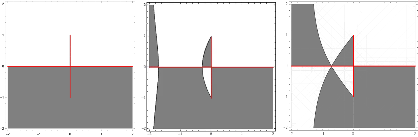
For \(\xi<0\), the two stationary points of the phase function \(\theta(\xi,k)\) are given by \[k_1(\xi) = \frac{1}{8}\left(\xi-\sqrt{\xi^2-\xi_c^2}\right), \qquad k_2(\xi) = \frac{1}{8}\left(\xi+\sqrt{\xi^2-\xi_c^2}\right). \label{eq:stationary}\tag{31}\] When \(\xi\le \xi_c\), both stationary points lie on the real axis. At the critical value \(\xi=\xi_c\), they coalesce at \[k_c=-\frac{q_o}{\sqrt{2}}.\] For \(\xi_c<\xi<0\), the two stationary points move off the real axis and form a complex conjugate pair. Since we restrict our analysis to \((x,t)\in\mathcal{P}_-\), it is enough to describe the sign distribution of \(\Re(\mathrm{i}\theta)\) for \(\xi\le \xi_c\); see Figure 2.

3.1 Opening of lenses↩︎

The purpose of this subsection is to perform a sequence of preliminary deformations of the original RH problem. These deformations consist mainly of opening lenses along the real axis. After these transformations, the resulting RH problem has the desired sign distribution: apart from the jumps on the branch cut and the jumps in small neighborhoods of the critical point \(k_c\), all jump matrices converge exponentially fast to the identity matrix as \(t\to\infty\).

First deformation. For \(\xi<\xi_c\), we first use the following factorizations of the jump matrix on the real axis. More precisely, \[V_1 = \begin{cases} V_2^{(1)}V_0^{(1)}V_1^{(1)}, & \operatorname{Re} k<k_1,\\[0.6ex] V_4^{(1)}V_3^{(1)}, & \operatorname{Re} k>k_c, \end{cases}\] where \[V_0^{(1)} = \begin{pmatrix} 1+r\bar r & 0\\[0.6ex] 0 & \dfrac{1}{1+r\bar r} \end{pmatrix},\] \[V_1^{(1)} = \begin{pmatrix} d^{-1/2} & \dfrac{d^{1/2}\bar r\,e^{2\mathrm{i}\theta t}}{1+r\bar r} \\[1.2ex] 0 & d^{1/2} \end{pmatrix}, \qquad V_2^{(1)} = \begin{pmatrix} d^{-1/2} & 0 \\[1.2ex] \dfrac{d^{1/2}r\,e^{-2\mathrm{i}\theta t}}{1+r\bar r} & d^{1/2} \end{pmatrix},\] \[V_3^{(1)} = \begin{pmatrix} d^{-1/2} & 0 \\[1.2ex] d^{-1/2}r\,e^{-2\mathrm{i}\theta t} & d^{1/2} \end{pmatrix}, \qquad V_4^{(1)} = \begin{pmatrix} d^{-1/2} & d^{-1/2}\bar r\,e^{2\mathrm{i}\theta t} \\[1.2ex] 0 & d^{1/2} \end{pmatrix}.\] We then introduce the first transformation as follows: \[M^{(1)}(x,t,k) = M(x,t,k) \begin{cases} \bigl(V_3^{(1)}\bigr)^{-1}, & k\in \mathcal{R}_1^{(1)},\\[0.6ex] \bigl(V_1^{(1)}\bigr)^{-1}, & k\in \mathcal{R}_2^{(1)},\\[0.6ex] V_2^{(1)}, & k\in \mathcal{R}_3^{(1)},\\[0.6ex] V_4^{(1)}, & k\in \mathcal{R}_4^{(1)}, \end{cases}\] were the regions \(\{\mathcal{R}_j^{(1)}\}_{j=1}^4\) are those shown in Figure 3.

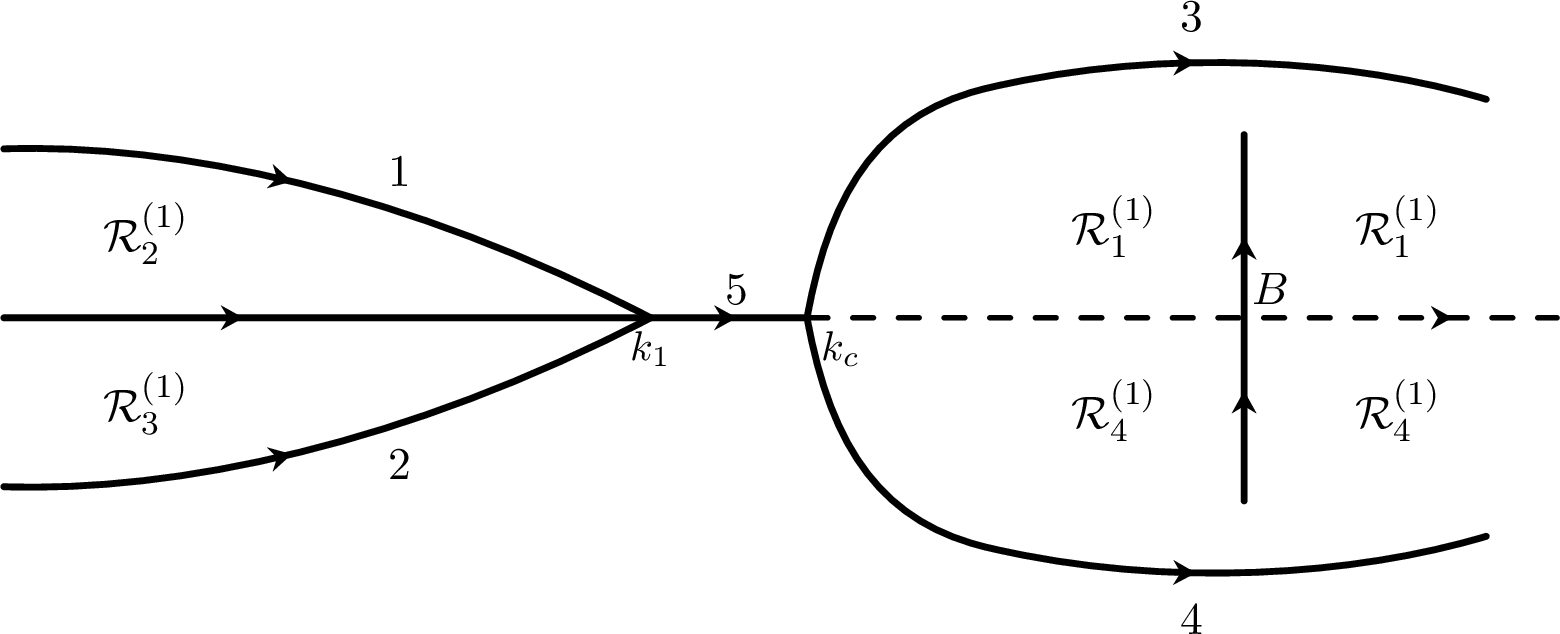
We denote the new jump contour by \(\Sigma^{(1)}\), and write the corresponding jump matrices as \(V^{(1)}\). On each component \(\Sigma_j^{(1)}\), the jump matrix is denoted by \(V_j^{(1)}\). The explicit expressions for \(V_j^{(1)}\), \(j=1,2,3,4\), are given above. On the branch cut \(B\), the jump matrix is \[\label{E:defVB} V_B^{(1)}=V_B = \begin{pmatrix} 0 & \dfrac{q_-}{\mathrm{i}q_o}\\[1.2ex] \dfrac{\bar q_-}{\mathrm{i}q_o} & 0 \end{pmatrix}.\tag{32}\] On \((-\infty,k_1)\), \(V^{(1)}(k)=V^{(1)}_0\). Moreover, on the remaining part of the real axis we have \(V^{(1)}_5(k)=V_1(k).\)

Second deformation. The second transformation is designed to remove the jump on \((-\infty,k_1)\). Define the scalar function \(\delta\) by \[\delta_+(k) = \delta_-(k)\bigl(1+r(k)\bar r(k)\bigr), \qquad k\in(-\infty,k_c),\] together with the normalization \[\delta(k)=1+O(k^{-1}), \qquad k\to\infty.\] Then \(\delta(k)\) can be solved explicitly via the Plemelj formulae \[\label{ds-delta-def} \delta( k) = \exp\left\{\frac{1}{2\mathrm{i}\pi}\int_{-\infty}^{k_c} \frac{\log \left[1+r(s)\bar r(s)\right]}{s-k} \, ds\right\}, \quad k\notin (-\infty, k_c).\tag{33}\] We then set \[M^{(2)}(x,t,k) = M^{(1)}(x,t,k)\delta(k)^{-\sigma_3}, \qquad k\in\mathbb{C}.\]

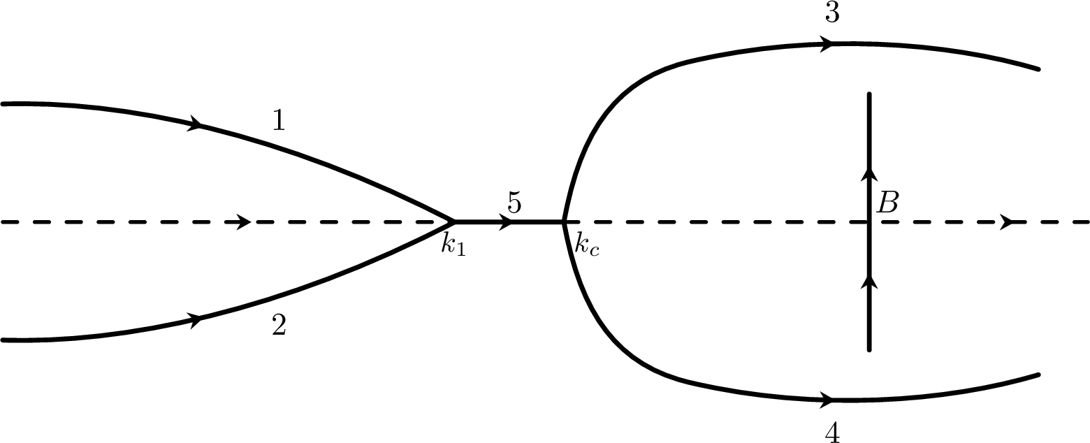
Let \(V^{(2)}\) denote the corresponding jump matrix. With this transformation, the jump on \((-\infty,k_1)\) is removed. The new jump contour is shown in Figure 3. The remaining jump matrices are given by \[\begin{align} V_B^{(2)} &= \begin{pmatrix} 0 & \dfrac{q_-}{\mathrm{i}q_o}\delta^2 \\[1ex] \dfrac{\bar q_-}{\mathrm{i}q_o}\delta^{-2} & 0 \end{pmatrix}, \qquad V_1^{(2)} = \begin{pmatrix} d^{-\frac{1}{2}} & \dfrac{d^{\frac{1}{2}}\bar r e^{2\mathrm{i}\theta t}}{1+r\bar r}\delta^2 \\[1.2ex] 0 & d^{\frac{1}{2}} \end{pmatrix}, \\[2ex] V_2^{(2)} &= \begin{pmatrix} d^{-\frac{1}{2}} & 0 \\[1.2ex] \dfrac{d^{\frac{1}{2}}r e^{-2\mathrm{i}\theta t}}{1+r\bar r}\delta^{-2} & d^{\frac{1}{2}} \end{pmatrix}, \qquad V_3^{(2)} = \begin{pmatrix} d^{-\frac{1}{2}} & 0 \\[1.2ex] d^{-\frac{1}{2}}r e^{-2\mathrm{i}\theta t}\delta^{-2} & d^{\frac{1}{2}} \end{pmatrix}, \\[2ex] V_4^{(2)} &= \begin{pmatrix} d^{-\frac{1}{2}} & d^{-\frac{1}{2}}\bar r e^{2\mathrm{i}\theta t}\delta^2 \\[1.2ex] 0 & d^{\frac{1}{2}} \end{pmatrix}, \qquad V_5^{(2)} = \delta_-^{\sigma_3}V_5^{(1)}\delta_+^{-\sigma_3}. \end{align}\]

Third deformation. The function \(d(k)\) can be eliminated from the jump matrices by introducing a new function \(N^{(3)}\) defined in terms of \(N^{(2)}\). Define \[\mathcal{R}_1^{(3)} := \mathbb{C}^+ \setminus \bigl(\mathcal{R}_1^{(1)}\cup\mathcal{R}_2^{(1)}\bigr), \qquad \mathcal{R}_2^{(3)} := \mathbb{C}^- \setminus \bigl(\mathcal{R}_3^{(1)}\cup\mathcal{R}_4^{(1)}\bigr).\] We set \[M^{(3)}(x,t,k) = M^{(2)}(x,t,k)D(k)=M^{(2)}(x,t,k) \times \begin{cases} d(k)^{\sigma_3/2}, & k\in \mathcal{R}_1^{(3)},\\[0.6ex] d(k)^{-\sigma_3/2}, & k\in \mathcal{R}_2^{(3)}. \end{cases}\] The jump contour \(\Sigma^{(3)}\) remains unchanged. We denote the corresponding jump matrix by \(V^{(3)}\). Its explicit form will be recorded below.

\[\begin{gather} V_1^{(3)}= \begin{pmatrix} 1&\dfrac{\bar r\mathrm{e}^{2\mathrm{i}\theta t}}{1+r\bar r}\,\delta^2\\[3mm] 0&1 \end{pmatrix}, \qquad V_2^{(3)}= \begin{pmatrix} 1&0\\[2mm] \dfrac{r\mathrm{e}^{-2\mathrm{i}\theta t}}{1+r\bar r}\,\delta^{-2}&1 \end{pmatrix},\\[3mm] V_3^{(3)}= \begin{pmatrix} 1&0\\[1mm] r\mathrm{e}^{-2\mathrm{i}\theta t}\delta^{-2}&1 \end{pmatrix}, \qquad V_4^{(3)}= \begin{pmatrix} 1&\bar r\mathrm{e}^{2\mathrm{i}\theta t}\delta^2\\[1mm] 0&1 \end{pmatrix},\\[3mm] V_5^{(3)} = \begin{pmatrix} 1 & \tfrac{\bar r e^{2\mathrm{i}\theta t}}{1+r\bar r} (\delta_+)^2 \\[1.4ex] \tfrac{r e^{-2\mathrm{i}\theta t} }{1+r\bar r} \tfrac{1}{(\delta_-)^2} & 1+r\bar r \end{pmatrix},\qquad V_B^{(3)}= \begin{pmatrix} 0&\dfrac{q_-}{\mathrm{i}q_o}\,\delta^2\\[2mm] \dfrac{\bar q_-}{\mathrm{i}q_o}\,\delta^{-2}&0 \end{pmatrix}. \end{gather} \label{eq:third-jumps}\tag{34}\]

Fourth deformation. Our final goal is to convert the jump along the branch cut \(B\) into the constant matrix \(V_B\) given by 32 . This can be achieved by means of the global transformation \[\label{ds-esc-n4-def-pw1} M^{(4)}(x, t, k) = M^{(3)}(x, t, k) e^{\mathrm{i}g( k)\sigma_3},\tag{35}\] where the function \(g(k)\) is analytic in \(\mathbb{C}\setminus B\) and satisfies the jump condition \[\label{ds-esc-jump-g-pw1} e^{\mathrm{i}(g^+ + g^-)} = \delta^2,\quad k\in B,\tag{36}\] and the normalization condition \[\label{ds-esc-g-rhp-pw1} \frac{g}{\lambda} = \mathcal{O}\left(\frac{1}{k}\right), \quad k \to\infty.\tag{37}\] Indeed, the jump condition 36 implies that the jump of \(M^{(4)}\) along \(B\) is precisely \(V_B\). Equations 36 and 37 formulate a RH problem for \(g\), which can be solved explicitly to yield \[\label{ds-esc-g-def-pw1} g( k) = \frac{\lambda(k)}{2 \mathrm{i}\pi^2} \int_{\zeta\in B} \frac{1}{\lambda(\zeta)\left(\zeta-k\right)} \int_{-\infty}^{k_c} \frac{\log \left[1+r(s)\bar r(s)\right]}{s-\zeta}\, ds d\zeta, \quad k\notin B.\tag{38}\] Notice that, after the above transformations, \(M^{(4)}\) is no longer normalized to the identity as \(k\to\infty\). Instead, we have \[M^{(4)}(x,t,k) = \left[I+O\left(k^{-1}\right)\right]e^{\mathrm{i}g_\infty\sigma_3}, \qquad k\to\infty,\] where \[\label{E:defginfty} g_\infty := \lim_{k\to\infty}g(k) = -\frac{1}{2\mathrm{i}\pi^2} \int_B \frac{1}{\lambda(\zeta)} \int_{-\infty}^{k_c} \frac{\log\left(1+|r(s)|^2\right)}{s-\zeta} \,ds\,d\zeta .\tag{39}\] It is important to note that one can directly verify that \(g_\infty\in\mathbb{R}.\)

The jump contour for \(M^{(4)}\) remains unchanged. The jump matrix \(V^{(4)}\) is as follows: \[\begin{align} V_1^{(4)}&= \begin{pmatrix} 1&\dfrac{\bar r\mathrm{e}^{2 \mathrm{i}(\theta t-g)}}{1+r\bar r}\,\delta^2\\[3mm] 0&1 \end{pmatrix}, \qquad V_2^{(4)}= \begin{pmatrix} 1&0\\[2mm] \dfrac{r\mathrm{e}^{-2 \mathrm{i}(\theta t-g)}}{1+r\bar r}\,\delta^{-2}&1 \end{pmatrix}, \\[3mm] V_3^{(4)}&= \begin{pmatrix} 1&0\\[1mm] r\mathrm{e}^{-2 \mathrm{i}(\theta t-g)}\delta^{-2}&1 \end{pmatrix}, \qquad V_4^{(4)}= \begin{pmatrix} 1&\bar r\mathrm{e}^{2 \mathrm{i}(\theta t-g)}\delta^2\\[1mm] 0&1 \end{pmatrix},\\[3mm] V_5^{(4)}& = \begin{pmatrix} 1 & \tfrac{\bar r e^{2\mathrm{i}(\theta t-g)}}{1+r\bar r} (\delta_+)^2 \\[1.4ex] \tfrac{r e^{-2\mathrm{i}(\theta t -g) } }{1+r\bar r} \tfrac{1}{(\delta_-)^2} & 1+r\bar r \end{pmatrix},\qquad V_B^{(4)}= \begin{pmatrix} 0 & \dfrac{q_-}{\mathrm{i}q_o}\\[1.2ex] \dfrac{\bar q_-}{\mathrm{i}q_o} & 0 \end{pmatrix}. \end{align}\]

3.2 The local parametrix and outer parametrix↩︎

In the previous subsection, after a sequence of contour deformations, all jump matrices were made exponentially close to the identity as \(t\to\infty\), except for the jumps on the branch cut and the jumps in a small neighborhood of the critical point \(k_c\). Therefore, two model constructions are needed. First, we construct a local parametrix in a neighborhood of \(k_c\). Second, we construct an outer parametrix which absorbs the nontrivial jump on the branch cut.

Local parametrix. We first record the Taylor expansion of the phase function near the critical point. Recall that \[\xi_c=-4\sqrt{2}\,q_o,\qquad k_c=-\frac{q_o}{\sqrt{2}}.\] Then, as \(k\to k_c\), \[\begin{align} \theta(\xi,k) ={}& \theta(\xi,k_c) +\frac{\xi+4\sqrt{2}\,q_o}{\sqrt{3}}(k-k_c) +\frac{4\sqrt{6}}{9q_o}(k-k_c)^3 \\ &\quad -\frac{\sqrt{6}}{9q_o}(\xi+4\sqrt{2}\,q_o)(k-k_c)^2 -\frac{2\sqrt{3}}{27q_o^2}(\xi+4\sqrt{2}\,q_o)(k-k_c)^3 +\mathcal{O}\bigl((k-k_c)^4\bigr), \end{align}\] where \[\label{E:thetaxikc} \theta(\xi,k_c) = 3\sqrt{3}\,q_o^2 -q_o\sqrt{\frac{3}{2}}\,(\xi-\xi_c).\tag{40}\] Equivalently, \[\theta(\xi,k) = \theta(\xi,k_c) +\frac{\xi-\xi_c}{\sqrt{3}}(k-k_c) +\frac{4\sqrt{6}}{9q_o}(k-k_c)^3 +S(\xi,k),\] where \[\label{E:Sdef} S(\xi,k) = -\frac{\sqrt{6}}{9q_o}(\xi-\xi_c)(k-k_c)^2 -\frac{2\sqrt{3}}{27q_o^2}(\xi-\xi_c)(k-k_c)^3 +\mathcal{O}\bigl((k-k_c)^4\bigr).\tag{41}\] We introduce the scaled variable \(z\) and \(y\) by \[\begin{align} z&= \left(\frac{8\sqrt{6}}{9q_o}\right)^{1/3} t^{1/3}(k-k_c),\\ y &= \frac{2}{\sqrt{3}} \left(\frac{8\sqrt{6}}{9q_o}\right)^{-1/3} t^{2/3}(\xi-\xi_c). \end{align}\] Let \(\mathcal{D}_{\epsilon}\) denote the open disk of radius \(\epsilon\) centered at the point \(k_c\). Then \(k \to z\) is a biholomorphism from \(\mathcal{D}_{\epsilon}\) onto the open disk of radius \(\left(\frac{8\sqrt{6}}{9q_o}\right)^{1/3} t^{1/3} \epsilon\) centered at the origin. With these definitions, we obtain \[\begin{align} 2t\bigl[\theta(\xi,k)-\theta(\xi,k_c)\bigr] &= yz+z^3+2tS(\xi,k), \qquad k \in \mathcal{D}_{\epsilon}. \end{align}\] Next we derive a local logarithmic representation of the scalar function \(\delta(z)\). Near \(k=k_c\), the local logarithmic representation is \[\delta(k) = (k-k_c)^{\mathrm{i}\nu} e^{\chi(k)}, \qquad k \in \mathcal{D}_{\epsilon},\] where \[\label{E:nu} \nu = -\frac{1}{2\pi} \log \left(1+|r(k_c)|^2\right),\tag{42}\] and \[\chi(k) = -\frac{1}{2\pi\mathrm{i}} \int_{-\infty}^{k_c} \log(k-\nu)\, \mathrm{d} \log\left(1+|r(\nu)|^2\right).\] Using \[k-k_c = \left(\frac{8\sqrt{6}}{9q_o}\right)^{-1/3} t^{-1/3}z,\] we have \[\begin{align} \delta(k)= \exp\left\{ -\frac{\mathrm{i}\nu}{3} \log\left(\frac{8\sqrt{6}}{9q_o}\right) -\frac{\mathrm{i}\nu}{3}\log t \right\} e^{\chi(k)} e^{\mathrm{i}\nu \log z}. \end{align}\]

We then decompose the factor \(\delta^2 e^{-2\mathrm{i}g}\) near the critical point \(k=k_c\). Using the local logarithmic representation of \(\delta\), for \(k \in \mathcal{D}_{\epsilon}\) we obtain \[\begin{align} \delta^2 e^{-2\mathrm{i}g} &= e^{2\mathrm{i}\nu\log z} \left( \frac{8\sqrt{6}}{9q_o}t \right)^{-\frac{2\mathrm{i}\nu}{3}} e^{2\chi(k_c)} e^{-2\mathrm{i}g(k_c)} \left[ e^{2(\chi(k)-\chi(k_c))} e^{-2\mathrm{i}g(k)+2\mathrm{i}g(k_c)} \right] = z^{2\mathrm{i}\nu}d_0d_1, \end{align}\] where \[d_0 = \left( \frac{8\sqrt{6}}{9q_o}t \right)^{-\frac{2\mathrm{i}\nu}{3}} \exp\left\{ 2\chi(k_c)-2\mathrm{i}g(k_c) \right\},\] and \[d_1 = \exp\bigl\{ 2\bigl(\chi(k)-\chi(k_c)\bigr) -2\mathrm{i}\bigl(g(k)-g(k_c)\bigr) \bigr\}.\]

We now introduce the local conjugating matrix \(Y\). Let \[\label{E:r0} r_0=|r(k_c)|, \qquad r(k_c)=r_0e^{\mathrm{i}\arg r(k_c)}.\tag{43}\] Define \[\label{E:Ydef} Y= \begin{pmatrix} e^{\mathrm{i}t\theta(\xi,k_c)} d_0^{1/2} e^{-\frac{\mathrm{i}}{2}\arg r(k_c)} & 0 \\[1ex] 0 & e^{\frac{\mathrm{i}}{2}\arg r(k_c)} e^{-\mathrm{i}t\theta(\xi,k_c)} d_0^{-1/2} \end{pmatrix}=:\begin{pmatrix} Y_1 & 0 \\[1ex] 0 & Y_1^{-1} \end{pmatrix}.\tag{44}\]

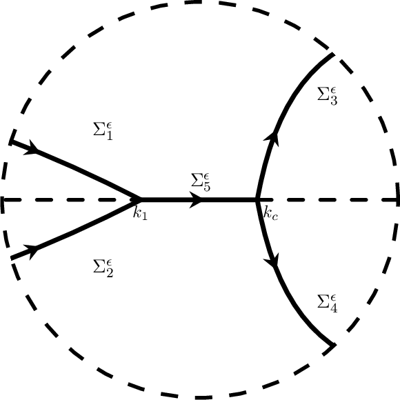
Set \[\widetilde{M}=M^{(4)}Y, \qquad k \in \mathcal{D}_{\epsilon}.\] Then the jump matrix of \(\widetilde{M}\) is \[\widetilde{V} = Y^{-1}V^{(4)}Y.\] The purpose of this conjugation is to remove the constant phase and amplitude factors in the local jumps. Define \(\Sigma^{\epsilon}=\cup_{j=1}^5 \Sigma^{\epsilon}_j\), where \(\Sigma^{\epsilon}_j=\Sigma^{(4)}_j \cap \mathcal{D}_{\epsilon}\); see Fig 5. Let \(\widetilde{V}^{\epsilon}_j\) denotes the restriction of \(\widetilde{V}\) to \(\Sigma^{\epsilon}_j\). For a fixed \(z\), as \(t \to \infty\) (this leads to \(k \to k_c\)), we know that \(\widetilde{V}^{\epsilon}_j(x,t,k)\) tends to the jump matrix \(V^{X}_j(x,t,z)\) defined in 56 for large \(t\).

Therefore, the local parametrix in the \(k\)-plane is defined by \[\label{E:Mloc} M^{\mathrm{loc}}(k) = Y M^X(z(k))Y^{-1}, \qquad k\in \mathcal{D}_\epsilon.\tag{45}\] We now show that \(M^{(4)}\) can be approximated by \(M^{\rm loc}\) in \(\mathcal{D}_\epsilon\).

Outer parametrix. In the present setting, the outer parametrix is the solution of the following Riemann–Hilbert problem: \[\begin{cases} M^{\mathrm{out}}_+(k) = M^{\mathrm{out}}_-(k)V_B(k), & k\in B, \\[0.8ex] M^{\mathrm{out}}(k) = \left(I+O(k^{-1})\right)e^{\mathrm{i}g_\infty\sigma_3}, & k\to\infty. \end{cases}\] This model problem has been explicitly solved in [12], [13]. More precisely, its solution is given by \[M^{\mathrm{out}}(k) = \frac{1}{2} e^{\mathrm{i}g_\infty\sigma_3} \begin{pmatrix} \Lambda(k)+\Lambda^{-1}(k) & -\dfrac{q_-}{q_o}\left(\Lambda(k)-\Lambda^{-1}(k)\right) \\[1.2ex] -\dfrac{q_o}{q_-}\left(\Lambda(k)-\Lambda^{-1}(k)\right) & \Lambda(k)+\Lambda^{-1}(k) \end{pmatrix},\] where \[\Lambda(k) = \left( \frac{k-\mathrm{i}q_o}{k+\mathrm{i}q_o} \right)^{1/4}.\] Here the fourth root is chosen so that \[\Lambda(k)\to 1, \qquad k\to\infty.\] Notice that \[\lim_{k\to\infty} k\left(\Lambda(k)-\Lambda^{-1}(k)\right) = -\mathrm{i}q_o.\] Therefore, \[\label{E:gjjx} \begin{align} -2\mathrm{i} \lim_{k\to\infty} \left[ k\left(M^{\mathrm{out}}(x,t,k)\right)_{12} \right] e^{\mathrm{i}g_\infty} &= -2\mathrm{i} \lim_{k\to\infty} \left[ -\frac{q_-}{2q_o} k\left(\Lambda(k)-\Lambda^{-1}(k)\right) e^{\mathrm{i}g_\infty} \right] e^{\mathrm{i}g_\infty} \\ &= q_-e^{2\mathrm{i}g_\infty}. \end{align}\tag{49}\] This limiting relation will be used later in the reconstruction formula.

3.3 The small norm RH problem↩︎

We define the final transformation to obtain a small-norm RH problem as follows: \[E(x,t,k) = \begin{cases} M^{(4)}(x,t,k)\bigl(M^{\mathrm{out}}(x,t,k)\bigr)^{-1}, & k\in \mathbb{C}\setminus \overline{\mathcal{D}_\epsilon}, \\[1.2ex] M^{(4)}(x,t,k) \bigl(M^{\mathrm{loc}}(x,t,k)\bigr)^{-1} \bigl(M^{\mathrm{out}}(x,t,k)\bigr)^{-1}, & k\in \mathcal{D}_\epsilon. \end{cases}\] The jump contour of \(E\) is \[\Sigma^E=\Sigma^{(4)}\cup \partial \mathcal{D}_\epsilon,\] where \(\partial \mathcal{D}_\epsilon\) is oriented counterclockwise. The corresponding jump matrix \(V^E\) is given by \[V^E(k) = \begin{cases} M^{\mathrm{out}}(k) \bigl(M^{\mathrm{loc}}(k)\bigr)^{-1} \bigl(M^{\mathrm{out}}(k)\bigr)^{-1}, & k\in \partial \mathcal{D}_\epsilon, \\[1.4ex] M^{\mathrm{out}}(k) V^{(4)}(k) \bigl(M^{\mathrm{out}}(k)\bigr)^{-1}, & k\in \Sigma^{(4)} \setminus\bigl(\overline{ \mathcal{D}_\epsilon}\cup B\bigr), \\[1.4ex] I, & k\in B, \\[1.4ex] M^{\mathrm{out}}(k) \left[ M_-^{\mathrm{loc}}(k) V^{(4)}(k) \bigl(M_+^{\mathrm{loc}}(k)\bigr)^{-1} \right] \bigl(M^{\mathrm{out}}(k)\bigr)^{-1}, & k\in \Sigma^{\epsilon}. \end{cases}\] Let \[w^E(k):=V^E(k)-I.\] The following estimates show that the error problem is a small-norm RH problem.

Consequently, \[\left\|w^E\right\|_{L^1(\Sigma^E)} \le C t^{-1/3}, \qquad \left\|w^E\right\|_{L^\infty(\Sigma^E)} \le C t^{-1/3}\log t.\] In particular, by interpolation, \(\left\|w^E\right\|_{L^2(\Sigma^E)} \le C t^{-1/3}(\log t)^{1/2}.\)

Define the Cauchy operator \[\mathcal{C}_{w^E}(h):=\mathcal{C}_-\bigl(hw^E\bigr).\] Since \(\|\mathcal{C}_{w^E}\|_{B(L^2(\Sigma^E))}\to 0\), \(t\to\infty\), the operator \(I-\mathcal{C}_{w^E}\) is invertible for sufficiently large \(t\). Thus we may define \[\mu^E = I+(I-\mathcal{C}_{w^E})^{-1} \mathcal{C}_{w^E}I \in I+L^2(\Sigma^E).\] We shall estimate \(\mu^E-I\). Indeed, \[\label{E:mujh} \begin{align} \|\mu^E-I\|_{L^2(\Sigma^E)} &\le \sum_{j=0}^{\infty} \| \mathcal{C}_{w^E}\|_{B(L^2(\Sigma^E))}^j \|\mathcal{C}_{w^E}I\|_{L^2(\Sigma^E)} \\ &\le \frac{ \|\mathcal{C}_-\|_{B(L^2(\Sigma^E))} \|w^E\|_{L^2(\Sigma^E)} }{ 1- \|\mathcal{C}_-\|_{B(L^2(\Sigma^E))} \|w^E\|_{L^\infty(\Sigma^E)} } \le C t^{-1/3}(\log t)^{1/2}. \end{align}\tag{50}\]

By the standard theory for small-norm RH problems, the error function \(E(x,t,k)\) can be represented as \[E(x,t,k) = I+\frac{1}{2\pi\mathrm{i}} \int_{\Sigma^E} \frac{\mu^E(x,t,s)w^E(x,t,s)}{s-k}\,ds, \qquad k\in\mathbb{C}\setminus\Sigma^E.\] Therefore, the coefficient of \(k^{-1}\) in the expansion of \(E\) at infinity is \[E^{(1)}(x,t) := \lim_{k\to\infty}k\bigl(E(x,t,k)-I\bigr)=-\frac{1}{2\pi\mathrm{i}} \int_{\Sigma^E} \mu^E(x,t,s)w^E(x,t,s)\,ds.\]

We next compute the contribution from \(\partial \mathcal{D}_\epsilon\). Recall that for \(k\in\partial \mathcal{D}_\epsilon\), \[w^E(x,t,k) = M^{\mathrm{out}}(x,t,k) \left[ \bigl(M^{\mathrm{loc}}(x,t,k)\bigr)^{-1}-I \right] \bigl(M^{\mathrm{out}}(x,t,k)\bigr)^{-1}.\] Therefore, by 48 and the residue theorem, \[\label{E:wedgj} \begin{align} -\frac{1}{2\pi\mathrm{i}} \int_{\partial \mathcal{D}_\epsilon} w^E(x,t,s)\,ds &= \frac{ M^{\mathrm{out}}(x,t,k_c) Y M_1^X(y) Y^{-1} \bigl(M^{\mathrm{out}}(x,t,k_c)\bigr)^{-1} }{ \left(\tfrac{8\sqrt{6}}{9q_o}\right)^{1/3} t^{1/3} } \\ &\quad + \mathcal{O}\left(t^{-2/3}\right), \qquad t\to\infty. \end{align}\tag{52}\] For convenience, write \[\label{E:defbetaj} M^{\mathrm{out}}(x,t,k_c) =: \begin{pmatrix} \beta_{11} & \beta_{12} \\ \beta_{21} & \beta_{22} \end{pmatrix}.\tag{53}\] Using formula 44 , 51 , 52 , 62  53 , a long but direct calculation gives \[\label{E:E12asyp} E^{(1)}_{12}(x,t) = - \frac{ \alpha_1\mathcal{V}(y) + \alpha_2\mathcal{V}^*(y) + \alpha_3\widehat{\mathcal{V}} (y) }{ \left(\tfrac{8\sqrt{6}}{9q_o}\right)^{1/3}t^{1/3} } + \mathcal{O}\left(t^{-2/3} \log t\right), \qquad t \to \infty,\tag{54}\] where \[\label{E:defalpha} \alpha_1=\beta_{12}^2 Y_1^{-2}, \qquad \alpha_2=\beta_{11}^2 Y_1^{2}, \qquad \alpha_3=2\beta_{11}\beta_{12}.\tag{55}\] Moreover, it is easy to see that \(\alpha_1(x,t)\), \(\alpha_2(x,t)\), and \(\alpha_3(x,t)\) are uniformly bounded quantities.

3.4 Proof of Theorem 1↩︎

We now use the reconstruction formula \[q(x,t) = -2\mathrm{i}\lim_{k\to\infty} kM_{12}(x,t,k)\] to compute the long-time asymptotics of \(q(x,t)\). Recalling all the invertible transformations introduced above, we have \[E(x,t,k) = M(x,t,k)\delta(k)^{-\sigma_3}D(k) e^{\mathrm{i}g(k)\sigma_3} \bigl(M^{\mathrm{out}}(x,t,k)\bigr)^{-1}.\] Therefore, \[M(x,t,k) = E(x,t,k)M^{\mathrm{out}}(x,t,k) e^{-\mathrm{i}g(k)\sigma_3} D^{-1}(k)\delta(k)^{\sigma_3}.\] Let \[M_{12}^{(1)}(x,t) := \lim_{k\to\infty}kM_{12}(x,t,k), \qquad \bigl(M^{\mathrm{out}}\bigr)_{12}^{(1)}(x,t) := \lim_{k\to\infty}kM_{12}^{\mathrm{out}}(x,t,k).\] Then the reconstruction formula gives \[q(x,t) = -2\mathrm{i}M_{12}^{(1)}(x,t)=-2\mathrm{i}E^{(1)}_{12}(x,t)-2\mathrm{i}\bigl(M^{\mathrm{out}}\bigr)_{12}^{(1)}(x,t)e^{\mathrm{i}g_{\infty}}.\] Using 54 and 49 , we arrive at \[q(x,t) = q_-e^{2\mathrm{i}g_\infty} + \frac{ 2\mathrm{i}\left[ \alpha_1\mathcal{V}(y) + \alpha_2\mathcal{V}^*(y) + \alpha_3\widehat {\mathcal{V}}(y) \right] }{ \left(\tfrac{8\sqrt{6}}{9q_o}\right)^{1/3}t^{1/3} } + \mathcal{O}\left(t^{-2/3}\log t\right).\] This is precisely the asymptotic formula 9 .

4 Concluding remarks↩︎

In this paper, we have studied the long-time asymptotics of the focusing NLS equation with symmetric NZBCs by using the Deift–Zhou nonlinear steepest descent method. The main contribution of the paper is twofold. First, we complete the Biondini–Mantzavinos long-time asymptotic picture by deriving the missing boundary-layer formula at the interface between the plane-wave and modulated elliptic-wave regions. Second, we show that this transition regime is governed by a distinguished tritronquée solution of an inhomogeneous Painlevé-II equation. Thus, the edge asymptotics of modulational instability are connected with the same type of Painlevé-II structure that is known to appear in the asymptotic analysis of rogue waves of infinite order. We hope that the present work will stimulate further research in this direction.

5 Painlevé II parametrix↩︎

Let \(\Sigma^X=\bigcup_{j=1}^5\Sigma_j^X\) be shown in Fig 6. Define \[\Phi(z;y):=yz+z^3.\] Let \(r_0>0\) and \(\nu<0\) be defined by 43 and 42 ,respectively. Define the jump matrix \(V^X(z)=V^X(y,z)\) by

\[V^X(z)=V_j^X(z), \qquad z\in \Sigma_j^X,\quad j=1,\ldots,5,\] where \[\label{E:Vjexp} \begin{align} V_1^X(z) &= \begin{pmatrix} 1 & \dfrac{r_0}{1+r_0^2} e^{\mathrm{i}\Phi(z;y)} z^{2\mathrm{i}\nu} \\[1.2ex] 0 & 1 \end{pmatrix},\qquad V_2^X(z) = \begin{pmatrix} 1 & 0 \\[1.2ex] \dfrac{r_0}{1+r_0^2} e^{-\mathrm{i}\Phi(z;y)} z^{-2\mathrm{i}\nu} & 1 \end{pmatrix},\\ V_3^X(z) &= \begin{pmatrix} 1 & 0 \\[1.2ex] r_0 e^{-\mathrm{i}\Phi(z;y)} z^{-2\mathrm{i}\nu} & 1 \end{pmatrix},\qquad V_4^X(z) = \begin{pmatrix} 1 & r_0 e^{\mathrm{i}\Phi(z;y)} z^{2\mathrm{i}\nu} \\[1.2ex] 0 & 1 \end{pmatrix}, \\ V_5^X(z) &= \begin{pmatrix} 1 & \dfrac{r_0}{1+r_0^2} e^{\mathrm{i}\Phi(z;y)} z_+^{2\mathrm{i}\nu} \\[1.2ex] \dfrac{r_0}{1+r_0^2} e^{-\mathrm{i}\Phi(z;y)} z_-^{-2\mathrm{i}\nu} & 1+r_0^2 \end{pmatrix}. \end{align}\tag{56}\] Then the local model RH problem is defined as follows:

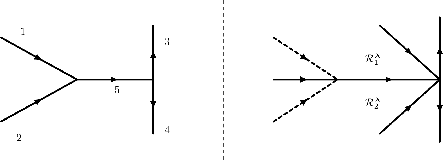
We introduce the following transformation: \[\label{E:widehatM} \widehat M^X(z) := M^X(z) z^{\mathrm{i}\nu\sigma_3} G(z),\tag{57}\] where \[G(z)= \begin{cases} \begin{pmatrix} 1 & -\dfrac{r_0}{1+r_0^2} \mathrm{e}^{\mathrm{i}\Phi (z,y)} \\[1.5ex] 0 & 1 \end{pmatrix}, & z\in \mathcal{R}_1^X, \\[4ex] \begin{pmatrix} 1 & 0 \\[1.5ex] \dfrac{r_0}{1+r_0^2} \mathrm{e}^{-\mathrm{i}\Phi(z,y)} & 1 \end{pmatrix}, & z\in \mathcal{R}_2^X, \\[4ex] I, & z\notin \mathcal{R}_1^X\cup \mathcal{R}_2^X. \end{cases}\] The regions \(\{\mathcal{R}_j^X\}_{j=1}^2\) are shown inb Fig. 6. Then \(\widehat M^X(z)\) can be expressed in terms of the solution of the following RH problem:

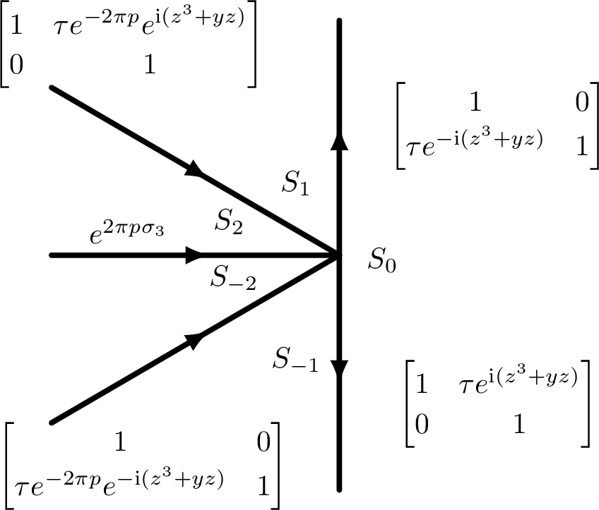
The RH problem above was studied systematically in Ref. [14]. In particular, it was shown there that, for all \(y,\tau, p \in\mathbb{R}\), the problem admits a unique solution. Moreover, the product \(W(z;y)z^{\mathrm{i}p\sigma_3}\) admits a complete asymptotic expansion \[\label{E:Wasy} W(z;y)z^{\mathrm{i}p\sigma_3} \sim I+\sum_{j=1}^{\infty} W_j(y) z^{-j}, \qquad z\to\infty,\tag{58}\] uniformly in all directions of the \(z\)-plane. In addition, define \[\mathcal{V}(y) := \lim_{z\to\infty} z \,W_{21}(z;y)z^{\mathrm{i}p} = ( W_1(y))_{21}.\] This function can be described in terms of a special solution of an inhomogeneous Painlevé-II equation. More precisely, there exists a unique tritronquée solution \(\mathcal{Q}(y)\) of \[\frac{d^2 \mathcal{Q}}{dy^2} + \frac{2}{3}y \mathcal{Q} - 2 \mathcal{Q}^3 - \frac{2}{3}\mathrm{i}p - \frac{1}{3} =0,\] which satisfies the asymptotic condition \[\mathcal{Q}(y) = \mathrm{i}\left(-\frac{y}{3}\right)^{1/2} - \left(\frac{1}{4}+\frac{\mathrm{i}p}{2}\right)\frac{1}{y} + O\left(|y|^{-5/2}\right), \qquad y\to-\infty.\] This solution is globally analytic for \(y\in\mathbb{R}\), and has trigonometric/algebraic asymptotic behavior as \(y\to+\infty\).

According to Ref. [14], the logarithmic derivative of \(\mathcal{V}(y)\) satisfies the above inhomogeneous Painlevé-II equation. More precisely, \[\mathcal{Q}(y)=\frac{\mathcal{V}'(y)}{\mathcal{V}(y)}.\] For \(y\to-\infty\), one has \[\begin{align} \mathcal{V}(y) &= \frac{\tau p\Gamma(\mathrm{i}p)}{2\sqrt{\pi}}\, e^{-\frac{\pi\mathrm{i}}{4}} e^{-\frac{\pi p}{2}} 2^{-\mathrm{i}p} e^{-2\mathrm{i}\left(-\frac{y}{3}\right)^{3/2}} (-y)^{-\frac{1}{4}-\frac{\mathrm{i}p}{2}} \left[1+O\left(|y|^{-5/4}\right)\right], \\ & y\to-\infty. \end{align}\] Thus, for \(y<0\), \(\mathcal{V}(y)\) can be written in the integral form \[\label{E:defmathcalV} \mathcal{V}(y) = C_{p,\tau} e^{-\frac{2}{9} \sqrt{3}\mathrm{i}\left(-y\right)^{3/2}} (-y)^{-\frac{1}{4}-\frac{\mathrm{i}p}{2}} \exp\left\{ \int_{-\infty}^{y} \left[ \mathcal{Q}(s) - \mathrm{i}\left(-\frac{s}{3}\right)^{1/2} + \left(\frac{1}{4}+\frac{\mathrm{i}p}{2}\right)\frac{1}{s} \right]\,ds \right\},\tag{59}\] where \[\label{E:MX1esp} C_{p,\tau} = \frac{\tau p\Gamma(\mathrm{i}p)}{2\sqrt{\pi}}\, e^{-\frac{\pi\mathrm{i}}{4}} e^{-\frac{\pi p}{2}} 2^{-\mathrm{i}p}.\tag{60}\] After the specialization \(p=-\nu\) and \(\tau=r_0\), we may write \[C_{p,\tau}=\alpha_0e^{\mathrm{i}\phi_0},\] with \[\alpha_0=|C_{p,\tau}|=\sqrt{-\frac{\nu}{2}}, \qquad \phi_0 = -\frac{\pi}{4} +\nu\log 2 +\arg\Gamma(-\mathrm{i}\nu).\]

We now apply these facts to the local model \(M^X\).

Acknowledgments↩︎

This work is supported by National Natural Science Foundation of China (Grant Nos. 12471234, 12471240, 12571268) and Science Foundation of Henan Academy of Sciences (Grant No. 20252319002).
Data sharing not applicable to this article as no datasets were generated or analyzed during the current study.

Declarations↩︎

Conflict of interest statement We declare that there is no conflict of interests.

References↩︎