Modeling and Analysis of Sensing Assisted UAV Networks for Urban Vehicular Communications
June 27, 2026
Abstract
Urban vehicular networks (VNs) demand seamless connectivity and situational awareness within road-constrained environments, motivating the deployment of unmanned aerial vehicles (UAVs) platforms capable of simultaneously sensing vehicles and establishing communication with them. In this paper, we present a sensing-assisted UAV network that provides connectivity to the vehicles in an urban area. The road network of the urban area is modeled as Manhattan Poisson line process (MPLP), and the random location of vehicles on each road is modeled as one dimensional Poisson point processes (PPPs). UAVs are distributed in the urban area at a fixed altitude and provide connectivity after sensing the vehicles. Their locations are modeled as a two-dimensional homogeneous PPP. Combined with the fixed altitude, this results in a three-dimensional spatial configuration. We incorporate an elevation dependent blockage model and define the sensing radius based on detection probability (DP), showing that it is jointly limited by signal strength and blockage effects. We derive the DP and characterize the typical UAV’s sensing region within the reliability requirements. We also derive the Laplace transform (LT) of aggregate interference accounting for directional patterns and sensing-driven activity, and analyze the resulting coverage probability (CP). Finally, we obtain the rate coverage (RC) of sensed vehicles falling within the UAV’s sensing zone. Numerical results shows that increasing altitude degrades sensing and coverage performance, whereas RC exhibits a non-monotonic trend, first decreasing and then increasing with altitude.
1 Introduction↩︎
Emerging urban 6G vehicular networks (VNs) supporting applications such as 3D map navigation, real-time traffic situational awareness, and cooperative driving, essentially demands reliable connectivity. The current infrastructure network is inadequate to reliably support these services, as high vehicular mobility and severe urban blockage conditions significantly degrade link reliability. To address these connectivity challenges low-altitude UAVs flying below 500 feet have gained significant attention as a key architectural component of future 6G-enabled VNs [1]–[4]. In particular, UAV-assisted VNs support high vehicular mobility by establishing reliable line-of-sight (LoS) links due to their flexible deployment, aerial mobility, and directional connectivity [5]–[9]. Moreover, beyond serving as aerial base stations or relays, next-generation UAVs are expected to support integrated sensing and communication (ISAC), enabling simultaneous detection, localization, and communication with vehicles [10], [11]. Recent advances in ISAC have highlighted the potential benefits of waveform co-design, beamforming, and spectrum sharing between sensing and communication tasks (see, e.g., [11]–[13]). In particular, sensing-assisted communication frameworks, in which sensing information is leveraged to adapt link design, are especially suitable for blockage-dominant THz 6G vehicular networks, where high mobility and severe propagation losses pose significant challenges [14]. These coupled effects are absent in conventional aerial base station models and remain insufficiently characterized in existing studies, thereby motivating a systematic analytical treatment tailored to urban vehicular low altitude wireless network (LAWN) deployments.
1.1 Related work↩︎
UAV-assisted vehicular networks (VNs) build on the broader foundation of UAV-enabled wireless communications. Comprehensive surveys have examined UAVs functioning as aerial base stations, relay nodes, and cellular users, characterizing their coverage, reliability, and latency performance [15]–[18]. These studies consistently highlight that downlink connectivity from aerial platforms is challenged by altitude-dependent channel characteristics, interference, and resource constraints. Unlike terrestrial base stations, UAVs offer flexible on-demand deployment and altitude-adaptive positioning, which are particularly valuable for serving vehicular users whose high mobility and unpredictable spatial distribution strain fixed ground infrastructure [19]. Within this context, recent work has addressed specific aspects of UAV deployment for vehicular connectivity. In [20], the coverage radius of UAV base stations was maximized by optimizing the UAV altitude, while [21] analyzed a UAV-assisted VN supporting both UAV-to-vehicle and vehicle-to-vehicle links, determining near-optimal UAV altitude to maximize the number of served users. An air-ground integrated VN was studied in [22], with emphasis on how UAV positioning affects task offloading performance. However, these works treat UAVs purely as communication nodes and do not exploit sensing information to improve link establishment or beam alignment.
| Reference | UAV | ISAC/ | Road | Stochastic | Blockage | Detection | Coverage/Rate | Beamwidth |
| Platform | Sensing | Topology | Geometry | Model | Prob. | Analysis | Trade-off | |
| [20] | ✔ | |||||||
| [21] | ✔ | ✔ | ||||||
| [2] | ✔ | 1D PPP | ✔ | ✔ | ||||
| [23] | PLP-PPP | ✔ | ✔ | |||||
| [24] | ✔ | ✔ | ✔ | |||||
| [25] | ✔ | ✔ | ✔ | ✔ | ||||
| [26] | ✔ | ✔ | ✔ | |||||
| [11] | ✔ | ✔ | Straight | ✔ | ✔ | |||
| This work | ✔ | ✔ | MPLP | ✔ | ✔ | ✔ | ✔ | ✔ |
In vehicular environments, especially at millimeter-wave and higher frequencies, establishing and maintaining directional links with fast-moving vehicles is extremely challenging. Sensing-assisted communication addresses this by using radar-derived
information such as vehicle location, speed, and direction to align beams proactively, eliminating the overhead of conventional beam training. This paradigm is central to ISAC, where the same hardware and spectrum resources are shared between radar sensing
and data transmission. Several studies have explored sensing integration into UAV platforms. In [24], a UAV-enabled ISAC framework jointly optimized trajectory and
target state estimation to balance sensing accuracy with communication throughput. The work in [25] optimized transmit beamforming for both quasi-stationary and mobile
UAV scenarios under sensing constraints, while [26] introduced a periodic sensing-and-communication protocol for adaptive power and frequency allocation. For vehicular
settings, [11] developed dynamic beamforming and trajectory optimization for UAV-vehicle tracking. While these contributions advance
UAV-ISAC design, they rely on optimization-based approaches for specific configurations and lack the scalable analytical characterization needed for system-level performance evaluation across diverse urban deployments. To enable such scalable analysis,
stochastic geometry (SG) has emerged as the primary mathematical framework for wireless network modeling. Line processes such as the Poisson line process and the Manhattan Poisson line process (MPLP) provide tractable models for random and grid-structured
urban road networks [27], [28]. Building on this
foundation, [23] modeled vehicular nodes as one-dimensional Poisson point processes distributed along roads generated by a Poisson
line process, forming a Cox process, and derived coverage probability (CP) expressions. In [2], UAV-assisted VNs were investigated using a simplified
one-dimensional PPP model that does not capture urban road structure.
1.2 Contributions:↩︎
This paper develops an analytical framework for sensing-assisted LAWN serving urban VNs. We quantify fundamental trade-offs between sensing reliability, CP, and interference. The main contributions are as follows.
An analytical framework is employed where roads are modeled as a MPLP, vehicles as \(1\)D Poisson point processes along roads, and UAVs as a \(2\)D Poisson point process. This captures the structured geometry of urban VNs and represents the analytical framework combining road-constrained vehicular distributions with aerial ISAC nodes.
The detection probability under directional radar sensing with altitude-dependent path-loss is derived. The sensing radius is shown to be limited by either SNR or LoS blockage, identifying two distinct operating regimes. The distribution of the nearest detected vehicle distance and the UAV activation probability are characterized, with an asymptotic analysis showing that in high-traffic environments the activation probability saturates, revealing that UAV-assisted connectivity is ultimately limited by sensing geometry rather than vehicular density.
The LT of aggregate interference is derived while accounting for stochastic UAV deployment, directional antenna patterns, and sensing-driven transmitter activity. This enables interference characterization under realistic sensing-assisted communication operation where UAV activity is coupled to sensing success. The CP is analyzed by conditioning on successful detection of the nearest vehicle, and the RC is derived accounting for multi-user load distribution. The framework quantifies the coupled impact of altitude, beamwidth, vehicular density, and UAV deployment density on communication performance.
Numerical results validate the analytical expressions and reveal fundamental trade-offs. The results provide system-level insights for the design of antenna patterns, deployment density, and altitude selection in sensing-assisted LAWN for urban VNs.
Notation: Notations used in this paper are summarized in notation Table 2. Here, we introduce only those notational definitions and transformations that cannot be concisely presented in the notation table. Each line \(\ell\) parallel to the \(\mathsf{x}\)- or \(\mathsf{y}\)-axis is uniquely identified by its perpendicular distance \(\rho\) from the origin. The base of a line \(\ell\) is defined as the point on \(\ell\) closest to the origin. For a fixed \(\rho \in \mathbb{R}\) and a one-dimensional coordinate \(\boldsymbol{x}\in \mathbb{R}\), the transformations \[\begin{align} \mathcal{T}_\mathsf{x}(\boldsymbol{x}) &= (\boldsymbol{x},\rho), \quad \mathcal{T}_\mathsf{y}(\boldsymbol{x}) = (\rho,\boldsymbol{x}), \end{align}\] map a one-dimensional location onto horizontal and vertical lines in \(\mathbb{R}^{2}\), respectively. These mappings are used to embed one-dimensional point processes into the two-dimensional plane. For a non-negative integer-valued random variable \(X\) with probability generating function (PGF) \(\mathcal{P}_{X}(s)\), we denote its first and second derivatives with respect to \(s\) as \(\mathcal{P}^{(1)}_{X}(s)\) and \(\mathcal{P}^{(2)}_{X}(s)\), respectively. The summation notation \(\sum_{\mathrm{N}_{k}}\) denotes summation over all \(k\)-tuples \((b_1,b_2,\ldots,b_m)\) of non-negative integers satisfying \(\sum_{i=1}^{m} i\,b_i = m\). This notation arises in higher-order derivative expansions of generating functions. For example, \(k=0\), \({\rm N}_{0}=\{(0)\}\), \(k=1\), \({\rm N}_1=\{(1)\}\), and \(k=2\), \({\rm N}_2=\{(2,0),(0,1)\}.\)
| Symbol | Description |
|---|---|
| \(\Phi_\ell\) | Road network modeled as MPLP with density \(\lambda_\ell\) |
| \(\Psi\) | Vehicle locations modeled as MPLP–PPP |
| \(\Phi_u\) | UAV locations as PPP with density \(\lambda_u\) |
| \(H\) | UAV altitude |
| \(\gamma\) | Antenna beamwidth |
| \(\mathbf{x}=(r,\theta)\) | Vehicle location \(\mathbf{x}\in\mathbb{R}^2\) in polar coordinates |
| \(d(r)\) | 3D UAV–vehicle distance \(\sqrt{r^2 + H^2}\) |
| \(r_{\mathrm{s}}, d_{\mathrm{s}}\) | Horizontal and 3D sensing radii |
| \(r_{\rm L}\) | Blockage-limited horizontal radius |
| \(r_{\rm s}^{\rm snr}\) | SNR-limited horizontal sensing radius |
| \(\alpha, \kappa_f\) | Path-loss exponent and absorption coefficient |
| \(G_\rms(\gamma)=G_\crm(\gamma)\) | Sensing/communication main-lobe gain |
| \(\sigma, \bar{\sigma}\) | Radar cross section and mean value |
| \(\tau_{\mathrm{s}}, \delta\) | Sensing SNR and reliability thresholds |
| \({\rm P_d}(r)\) | DP at distance \(r\) |
| \(N_0, \tau_c\) | Noise power and SINR threshold |
| \({\rm p_a}\) | UAV activation probability |
| \(N(r_{\mathrm{s}})\) | Number of vehicles in sensing zone |
| \(R_k\) | Distance to the \(k\)-th nearest vehicle |
| \({\rm P}_c^k(\tau_c)\) | CP of the \(k\)-th vehicle |
| \(r_c(\tau)\) | Rate CP |
| \(p_{\sf L}(r,H)\) | LoS probability at distance \(r\) and altitude \(H\) |
| \(\Lambda_{\rm h}(\rho), \Lambda_{\rm v}(\rho)\) | LoS-thinned vehicle counts on chord |
Definition 1 (MPLP). Let there be two independent \(1\)D PPPs, each with density \(\lambda_{\ell}\), defined on the representation space \(\mathbb{C}\equiv\mathbb{R}\times\{0,\pi/2\}\). The points with orientation \(0\) generate horizontal lines forming \(\Phi_{\rm h}\), while the points with orientation \(\pi/2\) generate vertical lines forming \(\Phi_{\rm v}\) in \(\mathbb{R}^{2}\). Taking the union of these two-line processes, \[\begin{align} \Phi_{\ell}=\Phi_{\rm h}\cup \Phi_{\rm v}, \end{align}\] constitutes a MPLP.
In MPLP, the number of horizontal (respectively, vertical) lines intersecting a convex region \(K\) is Poisson distributed with mean \(\lambda_{\ell}\,{\sf P}(K)\), where \({\sf P}(K)\) denotes the projection length of region \(K\) onto the \(\mathsf{y}\)-axis (respectively, the \(\mathsf{x}\)-axis).
Definition 2 (MPLP-PPP). Let \(\{\psi^{\rm h}_i,\; i\in\mathbb{N}\}\) and \(\{\psi^{\rm v}_j,\; j\in\mathbb{N}\}\) be two independent collections of i.i.d.\(1\)D PPPs on \(\mathbb{R}\), each with density \(\lambda\). The \(i\)th PPP \(\psi^{\rm h}_i\) is independently assigned to the \(i\)th horizontal line \(\ell_{i}\in\Phi_{\rm h}\), and the \(j\)th PPP \(\psi^{\rm v}_j\) is independently assigned to the \(j\)th vertical line \(\ell_{j}\in\Phi_{\rm v}\). Precisely, the mapped point processes are defined as \[\begin{align} &\Psi_{\rm h,\ell_{i}} = \bigcup\nolimits_{\boldsymbol{x}\in\psi^{\rm h}_{i}} \bigl\{ \mathbf{x}=\mathcal{T}_{\mathsf{x}}(\boldsymbol{x}) \bigr\}, \,\, \Psi_{{ \rm v},\ell_{j}} = \bigcup\nolimits_{\boldsymbol{x}\in\psi^{\rm v}_{j}} \bigl\{ \mathbf{x}=\mathcal{T}_{\mathsf{y}}(\boldsymbol{x}) \bigr\}. \end{align}\] The superposition of the transformed point processes on all horizontal and vertical lines yields \[\begin{align} \Psi_{\rm h}=\bigcup\nolimits_{\ell_{i}\in\Phi_{\rm h}}\Psi_{\rm h,\ell_{i}},\quad \Psi_{\rm v}=\bigcup\nolimits_{\ell_{j}\in\Phi_{\rm v}}\Psi_{{ \rm v},\ell_{j}}, \end{align}\] and the resulting point process \(\Psi=\Psi_{\rm h}\cup\Psi_{\rm v}\) is called the MPLP-PPP.
The remainder of this paper is organized as follows. Section II presents the system model, including road network modeling, UAV deployment, directional sensing, and communication models. Section III analyzes the sensing performance, deriving the DP, sensing radius, and UAV activation probability. Section IV presents the communication performance analysis, including interference characterization and coverage probability. Section V provides numerical results and insights. Section VI concludes the paper with future directions.
2 System Model↩︎
We consider an urban scenario where a fleet of UAVs is deployed at a common altitude \(H\) to provide downlink connectivity to ground vehicles. Each UAV operates sector-by-sector, it steers its directional beam to a sector, performs radar sensing to detect vehicles, and immediately communicates with any detected vehicles in that sector before advancing to the next. This sense-then-communicate cycle repeats across all \(2\pi/\gamma\) sectors spanning the full \(360^{\circ}\) azimuth. UAVs that detect no vehicle in any sector during the entire cycle remain idle and do not transmit, thereby reducing network interference. The key analytical objective is to characterize how the interplay among UAV altitude, antenna beamwidth, urban blockage, and road geometry governs the sensing reliability, UAV activation probability, and the resulting communication coverage and rate. In what follows, we present the spatial models for roads, vehicles, and UAVs, followed by the sensing model, the communication model, and the performance metrics.
2.1 Road network and vehicle model↩︎
The urban road network is modeled as an MPLP \(\Phi_\ell\) with line density \(\lambda_\ell\). MPLP accurately captures the Manhattan road structure, where roads run in two perpendicular directions forming the rectangular layout typical of urban cities. The MPLP model has been validated against real urban road networks [28]. This captures the road-constrained mobility of vehicles while preserving spatial randomness.
Vehicles on the roads of \(\Phi_\ell\) are modeled as an MPLP-PPP \(\Psi\), where vehicles on each road follow an independent \(1\)D PPP with density \(\lambda\). Each vehicle acts as a potential radar target for the UAVs. During the sensing phase, the UAV illuminates the ground with a directional radar beam to detect the presence and estimate the angular location of vehicles on the roads below. Upon detection, the UAV immediately reuses the beam alignment to establish a communication link, naturally coupling sensing and communication.
2.2 UAV deployment↩︎
The ground-projected locations of UAVs are modeled as a homogeneous \(2\)D PPP \(\Phi_u = \{\mathbf{y}_i,\, i \in \mathbb{N}\}\) with density \(\lambda_u\). The PPP model captures the spatial randomness inherent in on-demand UAV dispatches, where no predetermined positions are available. Assuming a fixed altitude \(H\), consistent with low-altitude airspace regulations, allows \(H\) to serve as a single tunable design parameter, consequently, the \(3\)D UAV–vehicle geometry is fully determined by the ground projection and altitude. Each UAV \(\mathbf{y}_i\) is assigned an independent mark \(\Theta_i\sim\mathrm{Unif}[0,2\pi)\) representing its starting scan angle, so that \(\tilde{\Phi}_u=\{(\mathbf{y}_i,\Theta_i)\}\) is an independently marked PPP [29] Once \(\Theta_i\) is drawn, the UAV’s sector grid is fixed and it scans sectors \(\Theta_i,\,\Theta_i+\gamma,\,\Theta_i+2\gamma,\,\ldots\) deterministically. Thus \(\Theta_i\) is the random rotational offset of the sector grid, and different UAVs have independently oriented grids. Without loss of generality the typical UAV at the origin we write \(\Theta_{\mathrm{o}}\), for an interfering UAV at \(\mathbf{y}\) we write \(\Theta_{\mathbf{y}}\).
2.3 Sensing model↩︎
Each UAV is equipped with a monostatic radar operating at carrier frequency \(f_c\) that uses a directional beam of angular width \(\gamma\) to detect ground vehicles. Because the beam illuminates only a fraction of the azimuth at any instant, the UAV performs a sequential angular scan in \(2\pi/\gamma\) discrete steps covering the full \(360^{\circ}\). Starting from \(\Theta_{\mathrm{o}}\), the typical UAV visits \(\Theta_{\mathrm{o},j} = \Theta_{\mathrm{o}}+j\gamma\) for \(j = 0, 1, \ldots, 2\pi/\gamma - 1\). In each step the boresight points in a fixed direction \({\Theta_{\mathrm{o},j}}\), and vehicles within the angular sector \([{\Theta_{\mathrm{o},j}}-\gamma/2,\,{\Theta_{\mathrm{o},j}}+\gamma/2]\) and within the maximum sensing range \(r_{\rm s}\) are potential detection targets. We refer to the region covered by a single step, the intersection of the disk of radius \(r_{\rm s}\) and the angular sector, as the instantaneous sensing zone. Since the full scan covers \(2\pi\), the sensing analysis (DP, sensing radius, activation probability) does not depend on the particular value of \(\Theta_{\mathrm{o}}\). We now describe the target fluctuation model, the path-loss model, the blockage model, and the antenna gain model that together determine the detection performance.
2.4 Swerling I target model↩︎
Each ground vehicle acts as a radar target whose echo signal fluctuates due to the vehicle’s complex shape and varying aspect angle relative to the UAV. We model these fluctuations using the Swerling I model [30], in which the radar cross section (RCS) \(\sigma\) follows an exponential distribution with mean \(\bar{\sigma}\), i.e., \(f_{\sigma}(\sigma)=\frac{1}{\bar{\sigma}}e^{-\sigma/\bar{\sigma}}\) for \(\sigma\geq 0\). The exponential distribution arises from
modeling the vehicle as a collection of many small, independently phased scatterers–a standard assumption in radar theory [31], [32]. Under Swerling I, the RCS remains constant during single scan but varies independently across scans. Importantly, the RCS distribution captures
the fluctuation statistics of the target reflectivity and is independent of the target’s distance from the UAV, the distance-dependent signal decay is captured separately by the path-loss model described next. A unified transmit power \(P_{\rm t}\) is used for both sensing and communication. The large-scale signal attenuation between a UAV and a ground vehicle is modeled as a combination of geometric spreading and frequency-dependent molecular absorption. At
the millimeter-wave carrier frequency considered here (\(f_c = 60\) GHz), oxygen molecules along the propagation path introduce absorption losses of approximately \(15\) dB/km [33], at lower carrier frequencies this term is negligible. Accordingly, the path-loss model is expressed as \[\begin{align} g(r)=
r^{-\alpha}\exp\!\left(-\kappa_f r\right),
\end{align}\]where \(\alpha\) denotes the path-loss exponent and \(\kappa_f\) represents the molecular absorption coefficient at the operating carrier frequency.
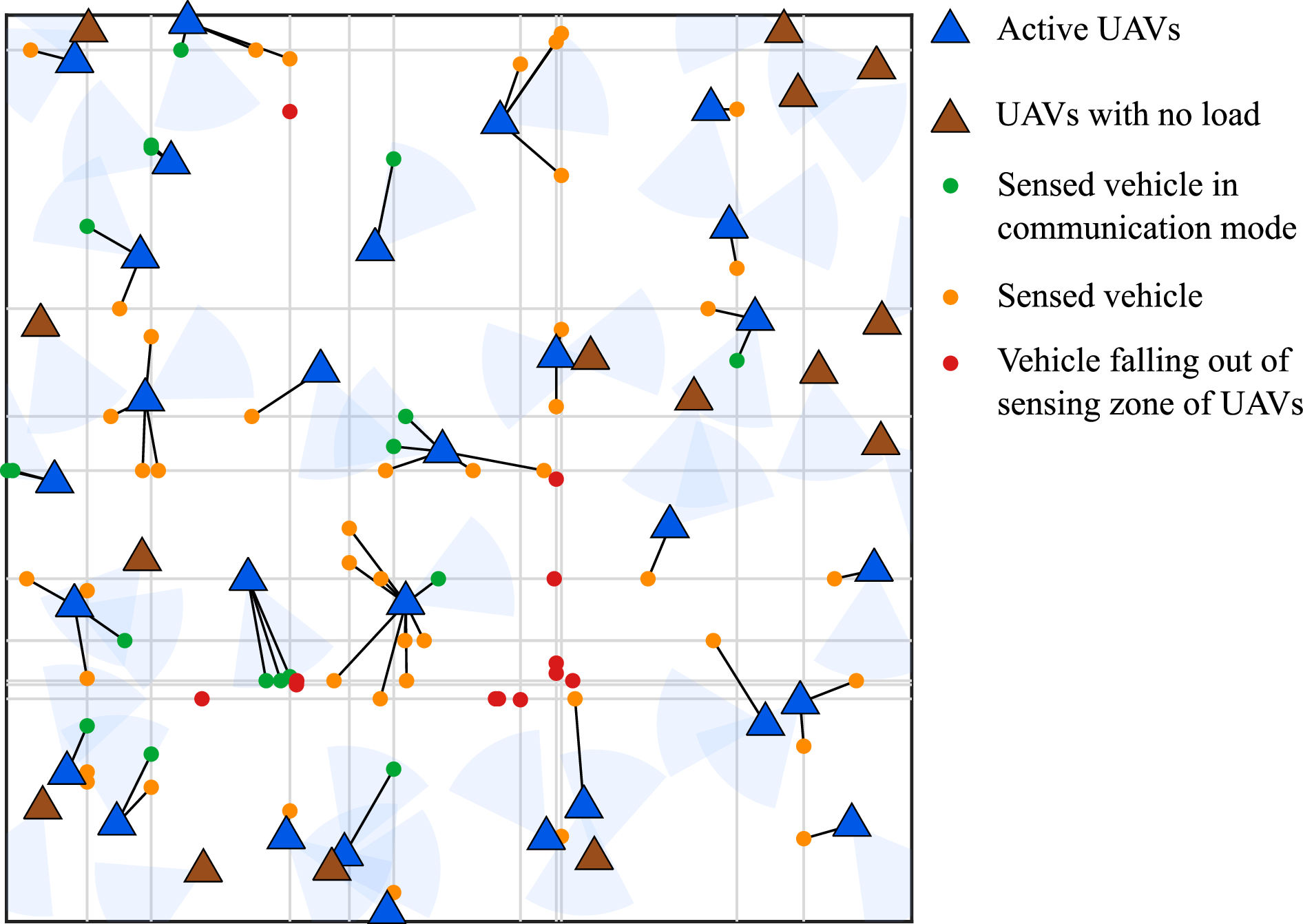
Fig. 1 illustrates the network layout. UAVs hover above a grid of urban roads on which vehicles are distributed. An active UAV is one that has detected at least one vehicle within its
sensing zone of radius \(r_{\rm s}\) during a full angular scan and is engaged in directional downlink communication. An inactive UAV has completed a full scan without detecting any vehicle and therefore does not transmit.
2.5 Blockage model↩︎
In UAV-to-vehicle communication, the probability of LoS depends on the elevation angle \(\theta_\mathrm{e}=\arctan(H/r)\), where \(H\) is the altitude of the UAV and \(r\) is the horizontal distance of the vehicle from the UAV. Unlike terrestrial blockage, which is primarily distance-dependent, UAV links experience a different blockage regime: the region directly below the UAV is almost certainly LoS, while at shallow elevation angles buildings increasingly obstruct the path. We adopt the widely used sigmoid LoS model [34] \[\label{eq:PLoS} { p}_{\sf L}(r,H) = \frac{1}{1 + a \exp\!\left(-b\!\left[\frac{180}{\pi}\arctan\!\left(\frac{H}{r}\right) - a\right]\right)},\tag{1}\] where \(a\) and \(b\) are environment-dependent parameters. The NLoS probability is simply \[p_{\sf N}(r,H) = 1 - p_{\rm L}(r, H).\]
Step-like nature of the blockage probability: A key property of the sigmoid LoS model in 1 is its step-like transition behavior as a function of the horizontal distance \(r\) for a fixed altitude \(H\). For small \(r\) (i.e., large elevation angles), the LoS probability \(p_{\sf L}(r,H) \approx 1\), implying near-certain LoS. As \(r\) increases beyond a critical distance, \(p_{\sf L}(r,H)\) drops sharply toward zero, exhibiting an approximate step-function transition. The steepness of this transition is governed by the parameter \(b\): larger values of \(b\) produce a sharper drop, making the LoS probability resemble a unit step function. Formally, in the limit \(b \to \infty\), the LoS probability reduces to a step function: \[\label{eq:PLoS95step} \lim_{b\to\infty} p_{\sf L}(r,H) = \begin{cases} 1, & \text{if } \arctan(H/r) > \frac{\pi a}{180},\\ 0, & \text{if } \arctan(H/r) < \frac{\pi a}{180}, \end{cases}\tag{2}\] which defines a blockage-limited radius \(r_{\rm L} = H/\tan(\pi a/180)\) beyond which LoS is effectively lost. This step-like behavior implies that beyond a certain horizontal range, the LoS path is almost entirely blocked by urban structures, regardless of the transmit power or antenna gain. Consequently, the effective sensing and communication range of the UAV is fundamentally limited by the urban blockage environment, not merely by signal attenuation.
Use of the blockage model: We employ the LoS model at two levels of approximation. For defining the blockage-limited sensing radius, we adopt the step-function limit in 2 , yielding the closed-form cutoff \(r_{\rm L}=H/\tan(\pi a/180)\). This is appropriate because the sensing radius is a hard design boundary, a vehicle is either within the reliable sensing range or not. For the communication analysis (interference characterization and CP), we retain the full sigmoid model 1 because interference is a statistical aggregate over all UAVs, and the smooth LoS transition accurately weights each interferer’s contribution.
2.6 Directional antenna gain model↩︎
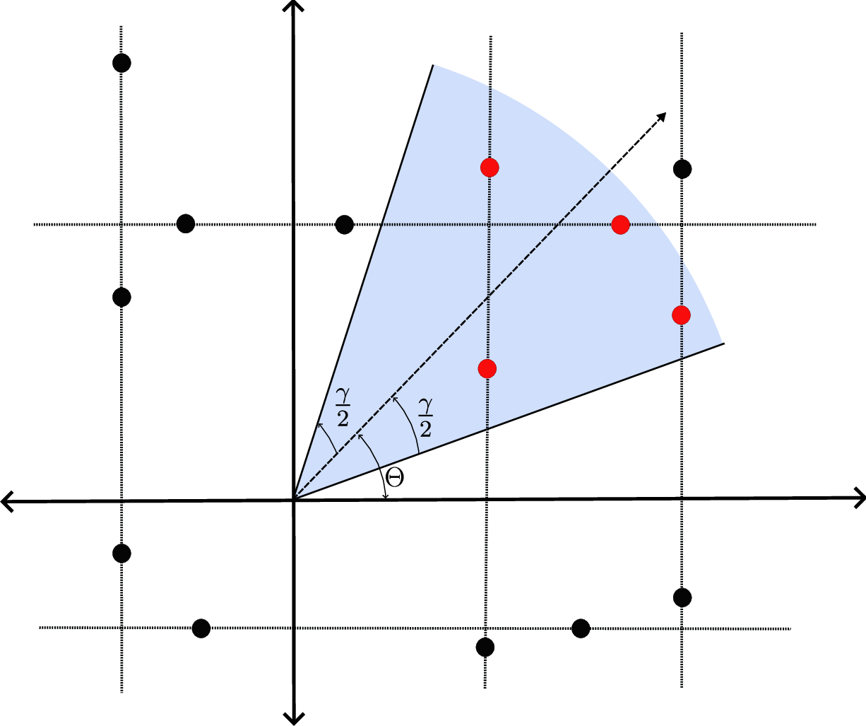
The sensing antenna is modeled using a sectored beam approximation with beamwidth \(\gamma\), which is widely adopted in ISAC enable LAWN analysis to capture main-lobe characteristics while maintaining analytical tractability [24]–[26]. As shown in Fig. 2, for the typical UAV at the origin and a vehicle at \(\mathbf{x}=(r,\theta)\), the effective sensing gain is \[\begin{align} \label{eq:Geff} G_{\mathrm{eff}}({\Theta_{\mathrm{o}}}) = \begin{cases} G_{{ \rm s}}(\gamma)={2\pi}/{(3\gamma)}, & \text{if }\;|\theta-{\Theta_{\mathrm{o}}}|\le \gamma/2, \\[1.2ex] 0, & \text{otherwise}, \end{cases} \end{align}\tag{3}\] where \({\Theta_{\mathrm{o}}}\) denotes the current boresight direction of the typical UAV. The main-lobe gain satisfies \(G\approx k/\gamma\), where the constant \(k=120^{\circ}= 2\pi/3\) corresponds to the standard approximation for a linear aperture [35], [36]. This sectored gain model is consistent with recent stochastic-geometry analysis of ISAC networks [37], [38]. Since \(G_{{ \rm s}}(\gamma)\) is a deterministic function of \(\gamma\), it scales the SNR by a fixed constant without affecting the independence structure, preserving analytical tractability.
For simplicity, we assume that the sidelobe gain is negligible, consistent with directional beamforming systems where the main-to-side lobe ratio exceeds 20 dB [39]. We note that the antenna model captures only the azimuthal beamwidth \(\gamma\), the elevation beampattern is assumed to be sufficiently broad to illuminate the ground at all relevant horizontal distances.
Without loss of generality, we place the typical UAV at the origin, i.e., \(\mathrm{o}\in \Phi_u\), and analyze the sensing and communication performance from its perspective. For a vehicle located at \({\boldsymbol{x}}=(r,\theta)\in\mathbb{R}^2\) relative to the UAV’s ground projection, the radar echo-based sensing signal-to-noise ratio (SNR) at the UAV is given by \[{\rm SNR}_{{ \rm s}}(d,\theta) = \frac{ P_{\rm t}\, G_{\mathrm{eff}}^2({\Theta_{\mathrm{o}}})\, \lambda_c^2 \, \sigma }{ (4\pi)^3 \, d^{2\alpha} \, N_0 } \exp\!\left(-2\kappa_f d\right),\]The factor \(\lambda_c^2/(4\pi)^3\) is the two-way radar path-loss constant, where \(d \triangleq d(r) = \sqrt{r^2+H^2}\) is the three-dimensional (slant) distance between the UAV at altitude \(H\) and a vehicle at horizontal distance \(r\), \(\lambda_c={c}/{f_c}\) is the carrier wavelength (\(c\) denotes speed of light, \(f_c\) denotes the carrier frequency), \(N_{0}\) is the additive white Gaussian noise (AWGN) power, and \(G_{\mathrm{eff}}({\Theta_{\mathrm{o}}})\) is the effective monostatic sensing gain defined in 3 .
Definition 3 (Detection probability). A vehicle at \(\mathbf{x}=(r,\theta)\) is successfully detected if \(\mathrm{SNR}_{{ \rm s}}(d(r),\theta)\ge \tau_{ \rm s}\), where \(\tau_{ \rm s}\) is the sensing threshold. The DP of a vehicle at distance \(r\) is \[\begin{align} {\rm P_d}(r)=\mathbb{P}[\mathrm{SNR}_{ \rm s}(d(r),\theta)\ge \tau_{ \rm s}]. \label{Pdr} \end{align}\qquad{(1)}\]
The SNR-threshold detection model is standard in radar theory where a target is declared present when the received echo exceeds the noise floor by a factor \(\tau_{{ \rm s}}\). When multiple vehicles fall within the same beam sector simultaneously, each vehicle generates an independent echo that can be resolved in range (time-delay) by the radar waveform. Cross-target interference from nearby vehicles is negligible at millimeter-wave frequencies due to the narrow beamwidth. We therefore model detections as independent across vehicles, conditioned on their respective distances. Since the UAV performs a full \(2\pi\) angular scan, every vehicle within horizontal distance \(r_{{ \rm s}}\) is guaranteed to be illuminated by the beam during the scan cycle. Consequently, the angular alignment factor \(\gamma/(2\pi)\) in the DP ?? is immaterial for determining the sensing range, the only relevant question is whether the SNR and LoS conditions are sufficient when the beam points at the vehicle. Therefore to define the maximum reliable sensing distance, we define the conditional DP as \[\begin{align} {\rm P_d^{cond}}(r)\triangleq p_{\sf L}(r,H)\,\exp\!\left(-\frac{\tau_s(4\pi)^3 d^{2\alpha} N_0\, e^{2\kappa_f d}}{P_t G_s^2(\gamma) \lambda_c^2 \bar\sigma}\right),\label{eq:Pd95cond} \end{align}\tag{4}\] where \(d\triangleq d(r)=\sqrt{r^2+H^2}\). To guarantee a minimum sensing reliability, we impose a conditional DP constraint and define the maximum reliable sensing radius as follows.
Definition 4 (Maximum reliable sensing distance). The maximum reliable horizontal sensing distance \(r_{ \rm s}\) is the largest horizontal distance at which a ground vehicle can be reliably detected, \[\begin{align} r_{\rm s} = \sup\!\big\{r \geq 0 : {\rm P_d^{cond}}(r) \geq \delta\big\},\label{eq:rs95def} \end{align}\qquad{(2)}\] where \(\delta\in(0,1)\) is the reliability threshold. Since \({\rm P_d^{cond}}(r)\) decreases monotonically in \(r\), the sensing radius is jointly constrained by the SNR and blockage limits, \[\begin{align} r_{\rm s} = \min\!\left(r_{\rm s}^{\rm snr},\; r_{\rm L}\right),\label{eq:rs95min} \end{align}\qquad{(3)}\] where \(r_{\rm s}^{\rm snr} = \sqrt{d_{\rm s}^2 - H^2}\) and \(r_{\rm L}=H/\tan(\pi a/180)\).
Definition 5 (UAV sensing zone). For the typical UAV during a single scan step with boresight direction \({\Theta_{\mathrm{o}}}\), the instantaneous sensing zone is defined as the set \[\mathcal{S}({\Theta_{\mathrm{o}}}) \triangleq \left\{ \mathbf{x}\in\Psi : r \le r_{ \rm s}, \; \left|\theta-{\Theta_{\mathrm{o}}}\right| \le {\gamma}/{2} \right\}, \label{eq:sensing95zone}\qquad{(4)}\] where \(\mathbf{x}=(r,\theta)\) denotes the location of a ground vehicle, \(r_{ \rm s}\) is the maximum reliable sensing distance, \({\Theta_{\mathrm{o}}}\) is the typical UAV’s antenna boresight direction, and \(\gamma\) is the antenna beamwidth. For an arbitrary UAV \(\mathbf{y}_i\) the sensing zone is \(\mathcal{S}(\Theta_i)\), with \(\Theta_i\) being its independent mark.
Since each UAV \(\mathbf{y}_i\) has an independent mark \(\Theta_i\), the overall sensing region is modeled as a Boolean process given by \[\mathcal{B} \triangleq \bigcup\nolimits_{\mathbf{y}_i\in\Phi_u} \left( \mathbf{y}_i + \mathcal{S}_i({\Theta_i}) \right),\]which represents the spatial region sensed by all the UAVs during the sensing phase. Note that the sensing set \(\mathcal{S}\) is convex, being the intersection of a disk and an angular sector. Hence, each translated set \(\mathbf{y}_i+\mathcal{S}\) is also convex.
2.7 Communication model↩︎
Within each sector, immediately after sensing, the UAV communicates with the detected vehicles using the beam alignment just obtained. If \(L\) vehicles were detected in that sector, the UAV allocates \(B/L\) of its bandwidth to each. Sectors with no detection are skipped. Because the beam illuminates one sector at a time, vehicles in different sectors do not compete for bandwidth simultaneously. We now characterize the
communication link model and the performance metrics.
3 Sensing Analysis↩︎
We first derive the DP and the maximum reliable sensing distance. Without loss of generality, we assume that the typical UAV is located at the origin.
Theorem 1. For a vehicle located at distance \(r\) from the typical UAV, the blockage-aware detection probability under directional sensing is given by (for proof see Appendix 7) \[\begin{align} {\rm P_{d}}(r) =\frac{\gamma}{2\pi}\; p_{\sf L}(r,H) \;\exp\!\left(-\frac{\tau_s(4\pi)^3 d^{2\alpha} N_0\, e^{2\kappa_f d}}{P_t G_s^2(\gamma) \lambda_c^2 \bar\sigma}\right),\label{detectionprobability} \end{align}\qquad{(5)}\] where \(d=\sqrt{r^2+H^2}\) and \(p_{\sf L}(r,H)\) is the LoS probability given in 1 . The factor \(p_{\sf L}(r,H)\) reflects the requirement that the radar round-trip must traverse a LoS path, vehicles in NLoS experience round-trip attenuation that renders negligible detection .
Remark 1 (Role of blockage in DP). The DP in ?? is the product of three terms: (i) the angular alignment probability \(\gamma/(2\pi)\), (ii) the LoS probability \(p_{\sf L}(r,H)\), and (iii) the exponential SNR decay. Among these, the LoS probability introduces a distance-dependent ceiling on the DP that is independent of the transmit power. Due to the step-like behavior of \(p_{\sf L}(r,H)\) described in 2 , the DP exhibits a sharp cutoff at the blockage-limited distance \(r_{\rm L}\), beyond which detection becomes negligible regardless of the radar power budget.
Theorem 2. The maximum horizontal sensing radius \(r_{\rm s}\) for a UAV at altitude \(H\) is \[\begin{align} r_{\rm s} = \min\!\left(\sup\!\big\{r \geq 0 : {\rm P_d^{cond}}(r) \geq \delta\big\},\; r_{\rm L}\right), \end{align}\] where \({\rm P_d^{cond}}(r)\) is defined in 4 and \(r_{\rm L}=H/\tan(\pi a/180)\) is the blockage-limited radius from 2 . The SNR-limited radius \(r_{\rm s}^{\rm snr}=\sqrt{d_{\rm s}^2-H^2}\) is the power-limited radius with \(d_{\rm s}\) satisfying \[\begin{align} d_{{ \rm s}} = \frac{\alpha}{\kappa_f} \,{\rm W}\!\left( \frac{\kappa_f}{\alpha} \left( \frac{-\ln(\delta)\, P_{\rm t}G_s^2(\gamma) \lambda_c^2}{\tau_{{ \rm s}} (4\pi)^3 N_0} \right)^{\frac{1}{2\alpha}} \right), \end{align}\]and consequently \(r_{\rm s}=\min(r_{\rm s}^{\rm snr},\, r_{\rm L})\). (For proof see Appendix 8.)
Remark 2. The sensing radius \(r_{\rm s} = \min(r_{\rm s}^{\rm snr}, r_{\rm L})\) identifies two regimes. In the blockage-dominant regime (\(r_{\rm L} < r_{\rm s}^{\rm snr}\)), urban obstructions limit sensing range before SNR becomes insufficient, which is common at low altitudes in dense areas where increasing transmit power yields no gain. In the SNR-dominant regime* (\(r_{\rm s}^{\rm snr} < r_{\rm L}\)), path loss and molecular absorption are the bottleneck, occurring at higher altitudes with large elevation angles. The transition is governed by altitude \(H\) and environment parameters \((a,b)\). In the blockage-dominant regime altitude should be increased to widen the LoS cone whereas in the SNR-dominant regime altitude should be minimized to reduce path loss.*
We first present the result for beamwidth \(0<\gamma<\pi\), we then present a generalize result when \(\gamma=2\pi\) that is the UAV equipped with an omnidirectional antenna.
Theorem 3. The probability generating function (PGF) of the number of detectable vehicles \(N(r_{{ \rm s}})\) falling within the sector sensing region of radius \(r_{{ \rm s}}\) around the typical UAV is given by (for proof sec Appendix 9) \[\begin{align} \mathcal{P}_{N(r_{{ \rm s}})}(s) &= \exp\!\big( g_\gamma(s,r_{{ \rm s}}) \big), \end{align}\] where \[\begin{align} &g_\gamma(s,r_{{ \rm s}})= \lambda_{\ell} \left[2 \int_{0}^{r_{\rm s}\sin(\gamma/2)} \left( \exp\!\left(\Lambda_{\rm h}(\rho)(s-1)\right)-1\right)\, \mathrm{d}\rho\right. \nonumber\\ &\left.\qquad + \int_{0}^{r_{\rm s}} \left( \exp\!\left(\Lambda_{ \rm v}(\rho)(s-1)\right)-1\right)\,\mathrm{d}\rho \right], \end{align}\]and the average number of vehicle on each chord are \[\begin{align} &\Lambda_{\rm h}(\rho) = \int_{\ell_{\rm h}(\rho,\gamma)} \lambda\; p_{\sf L}\!\big(\!\sqrt{x^2+\rho^2},\,H\big)\;\mathrm{d}x, \label{Lambdah} \\ &\Lambda_{ \rm v}(\rho) = \int_{\ell_{ \rm v}(\rho,\gamma)} \lambda\; p_{\sf L}\!\big(\!\sqrt{\rho^2+y^2},\,H\big)\;\mathrm{d}y.\label{Lambdav} \end{align}\] {#eq: sublabel=eq:Lambdah,eq:Lambdav} The chord limits \(\ell_{\rm h}(\rho,\gamma)\) and \(\ell_{ \rm v}(\rho,\gamma)\) have lengths \[\begin{align} &|\ell_{ \rm v}(\rho,\gamma)| = 2\,\min\!\left( \sqrt{r_s^{2}-\rho^{2}}, \; \rho\,\tan\!\left({\gamma}/{2}\right) \right), \label{vchord} \\ &|\ell_{\rm h}(\rho,\gamma)| = \sqrt{r_{\rm s}^{2}-\rho^{2}} - \rho\,\cot \!\left({\gamma}/{2}\right).\label{hcord} \end{align}\] {#eq: sublabel=eq:vchord,eq:hcord} When \(p_{\sf L}\equiv 1\) (no blockage), \(\Lambda_{\rm h}(\rho)\) reduces to \(\lambda|\ell_{\rm h}(\rho,\gamma)|\), recovering the original expressions.
Using the PGF, we can derive the PMF and perform the statistical analysis of the sensing load \(N({r_{ \rm s}})\)
Corollary 1. The PMF \(\mathbb{P}\left({N}(r_{{ \rm s}})=k\right)\) of the sensing load \({N}(r_{\rm s})\) on the typical UAV \[\begin{align} &p_{k}(r_{{ \rm s}})=\mathbb{P}\left({N(r_{{ \rm s}})}=k\right)\notag\\ &=e^{f_{0}(r_{{ \rm s}})}\sum\nolimits_{\mathrm{N}_{k}}\frac{\left(f_{1}(r_{{ \rm s}})\right)^{n_{1}}\cdots\left(f_{m}(r_{{ \rm s}})\right)^{n_{m}}}{n_{1}!\cdots n_{m}!},\label{PMF}\\ &\text{where }f_{0}(r_{{ \rm s}})={g(0,r_{{ \rm s}})}, \quad f_{m}(r_{{ \rm s}})={g^{(m)}(0,r_{{ \rm s}})}/{m!},\text{ with}\notag\\ & g^{(m)}(0,r_{{ \rm s}})= \lambda_{\ell}\left[ 2\int_{0}^{r_{\rm s}\sin(\gamma/2)} \big(\Lambda_{\rm h}(\rho)\big)^m e^{-\Lambda_{\rm h}(\rho)}\,\mathrm{d}\rho\right. \nonumber\\ &\left.+\int_{0}^{r_{\rm s}} \big(\Lambda_{\rm v}(\rho)\big)^m e^{-\Lambda_{\rm v}(\rho)}\,\mathrm{d}\rho \right], \end{align}\qquad{(6)}\] where \(\Lambda_{\rm h}(\rho)\) and \(\Lambda_{\rm v}(\rho)\) are the LoS-thinned chord counts from ?? –?? .
Corollary 2. The CDF of the distance of the \(n\)th nearest vehicle from the UAV is \(F_{R_{n}}(r)=\)
\[\begin{align} 1-\sum\nolimits_{k=0}^{k-1}e^{f_{0}(r)}\sum\nolimits_{\mathrm{N}_{k}}\frac{\left(f_{1}(r)\right)^{n_{1}}\cdots\left(f_{m}(r)\right)^{n_{m}}}{n_{1}!\cdots n_{m}!}\label{CDFRn} \end{align}\qquad{(7)}\] The PDF of the distance \(R_n\) of the \(n\)th nearest vehicle from the UAV is given by \[\begin{align} f_{R_n}(r) = -\sum\nolimits_{k=0}^{n-1}\frac{\mathrm{d}}{\mathrm{d}r}p_k(r). \label{PDFRn} \end{align}\qquad{(8)}\]
Using the CDF of the \(n\)th nearest vehicle, we now present the CDF and PDF for the nearest vehicle from the UAV in the following corollary.
Corollary 3. For the nearest detectable vehicle \(R_1\), the CDF and PDF are given by \[\begin{align} F_{R_{1}}(r) = 1 - e^{f_{0}(r)},\,\, f_{R_{1}}(r) = -f^{(1)}_{0}(r)e^{f_{0}(r)},\\ \text{where }f_{0}(r) = \lambda_{\ell} \Bigg[ 2 \int_{0}^{r\sin(\gamma/2)} \left( e^{-\Lambda_{\rm h}(\rho)} -1 \right) \mathrm{d}\rho \nonumber\\ \qquad + \int_{0}^{r} \left( e^{-\Lambda_{\rm v}(\rho)} -1 \right) \mathrm{d}\rho \Bigg], \end{align}\] and \(f^{(1)}_{0}(r) = \frac{\mathrm{d}}{\mathrm{d}r}f_0(r)\), where \(\Lambda_{\rm h}(\rho)\) and \(\Lambda_{\rm v}(\rho)\) are the LoS-thinned chord counts from ?? –?? evaluated with the sensing sector of radius \(r\).
The following corollaries translate the distance distributions derived above into operationally relevant sensing metrics for the typical UAV. Let the distance of the nearest and \(n\)th nearest vehicle from the typical UAV is denoted as \(R_{1}\) and \(R_{n}\). This can be directly obtained using the CDF of \(R_{n}\) presented in ?? .
Corollary 4. The probability that the nearest and \(k\)th nearest vehicle falls under the sensing zone of the typical UAV is \[\begin{align} \mathbb{P}\left(R_{1}\leq r_{\rm s}\right)=F_{R_{1}}(r_{\rm s}),\,\, \mathbb{P}\left(R_{n}\leq r_{\rm s}\right)=F_{R_{n}}(r_{\rm s}) \end{align}\]
Corollary 5. The PGF of the number of detectable vehicles located within the UAV sensing region \(\mathbf{b}_{2}(\mathbf{o}, r_{\rm s})\) for \(\gamma = 2\pi\), corresponding to an omnidirectional antenna. \[\begin{align} &\mathcal{P}_{{N}(r_{{ \rm s}})}(s)=\exp{\left(g_{2\pi}(s,r_{{ \rm s}})\right)},\\ &\text{where}\quad g_{2\pi}(s,r_{{ \rm s}})= 4\lambda_{\ell}\left(\int_{0}^{r_{{ \rm s}}}e^{\Lambda(\rho)(s-1)}\mathrm{d}\rho-r_{{ \rm s}}\right),\nonumber\\ &\text{with}\quad \Lambda(\rho)= 2\int_{0}^{\sqrt{r_{{ \rm s}}^{2}-\rho^{2}}}\lambda\, p_{\sf L}\!\big(\!\sqrt{x^2+\rho^2},H\big)\mathrm{d}x.\nonumber \end{align}\]
Corollary 6. The probability that no vehicle is present within the sensing region \[\begin{align} &{\rm p}_{\rm idle}=\mathbb{P}\left[{N}(r_{{ \rm s}})=0\right]=\exp{\left(4\lambda_{\ell}\left(\int_{0}^{r_{{ \rm s}}}e^{-\Lambda(\rho)}\mathrm{d}\rho-r_{{ \rm s}}\right)\right)}, \end{align}\]where \(\Lambda(\rho)= 2\int_{0}^{\sqrt{r_{{ \rm s}}^{2}-\rho^{2}}}\lambda\, p_{\sf L}(\sqrt{x^2+\rho^2},H)\mathrm{d}x\).
| Parameter | Value |
|---|---|
| Vehicle intensity, \(\lambda\) | \(30~\si{vehicles/km}\) |
| Road density, \(\lambda_l\) | \(2~\si{roads/km}\) |
| UAV altitude, \(H\) | \(100~\si{m}\) |
| UAV density, \(\lambda_u\) | \(5~\si{UAV/km^2}\) |
| Transmit power, \(P_t\) | \(1\) (normalized) |
| Sensing/comm.gain, \(G_s(\gamma){=}G_c(\gamma)\) | \(2\pi/(3\gamma)\) |
| Carrier wavelength, \(\lambda_{\rm c}\) | \(0.005~\si{m}\) |
| Noise power, \(N_0\) | \(10^{-9}\) |
| Sensing SNR threshold, \(\tau_{\rm s}\) | \(1\) |
| Mean fading power, \(\bar{\sigma}\) | \(1\) |
| Absorption coefficient, \(\kappa_f\) | \(3.45~\text{Np/km}\) [33] |
| Path-loss exponent, \(\alpha\) | \(2.2\) |
| LoS parameters (\(a\), \(b\)): | |
| Suburban | \(4.88,\;0.43\) |
| Urban | \(12.08,\;0.11\) |
| Dense Urban | \(9.61,\;0.16\) |
| High-rise Urban | \(27.23,\;0.08\) |
Hence the UAV activation probability is \({\rm p_{a}}=1-{\rm p}_{\rm idle}\). Observe that \({\rm p}_{\rm idle}\) is governed primarily by whether any road from the MPLP intersects the UAV’s sensing disk of radius \(r_{\rm s}\): if no road passes through the disk, no vehicle can be present regardless of the vehicular density \(\lambda\). Consequently, the activation probability depends on the UAV’s position relative to the road layout, captured through the line density \(\lambda_{\ell}\) and the sensing radius \(r_{\rm s}\).
Remark 3. As \(\lambda \to \infty\), the integral term vanishes and the idle probability converges to \(\exp(-4\lambda_{\ell} r_s)\). Consequently, the UAV activation probability saturates at \[\begin{align} \lim\nolimits_{\lambda \to \infty} {\rm p_{a}} = 1 - \exp\!\left(-4\lambda_{\ell} r_s\right).\label{asym} \end{align}\qquad{(9)}\] This limit equals the probability that at least one road from the MPLP intersects the UAV’s sensing disk of radius \(r_{\rm s}\). When vehicles are abundant, every road that crosses the disk contains at least one vehicle, hence the bottleneck is whether any road is present at all.
Having characterized the sensing metrics—DP, sensing radius, vehicle count distribution, and activation probability—we now analyze the communication performance of the detected vehicles.
4 Communication Analysis↩︎
In the communication phase of each sector, the active UAV steers its directional beam using the angular location obtained from the immediately preceding sensing step. A detected vehicle is served by its nearest active UAV, all other active UAVs whose beams happen to illuminate the vehicle contribute to interference. Hence we now present the CP for the nearest and \(k\)th nearest vehicle from the typical UAV. Let the nearest and the \(k\)th nearest vehicle is located at the \(\mathbf{x}_{1}\) and \(\mathbf{x}_{k}\). Not that the nearest and the \(k\)th nearest vehicle may be located on the same or the different road. For the \(k\)-th nearest vehicle located at \(\mathbf{x}_{k}\), the aggregate LoS-only interference is given by \[\begin{align} I_k&=\sum_{\mathbf{y}\in \Phi_u^{\rm a}\setminus \mathbf{b}_{2}(\mathbf{x}_k,r_k)} P_\mathrm{t}\, G_{\mathbf{y}}\, h_{\mathbf{y}}\, d(\|\mathbf{y}-\mathbf{x}_{k}\|)^{-\alpha}\notag\\ &\exp{\left(-\kappa_f d(\|\mathbf{y}-\mathbf{x}_{k}\|)\right)}\,\mathbb{1}(\text{LoS}), \end{align}\]where \(\mathbb{1} (\text{LoS})\) is a Bernoulli indicator with probability \(p_{\sf L}(\|\mathbf{y}-\mathbf{x}_k\|,H)\), reflecting that only LoS interferers contribute meaningfully.
Theorem 4. The LT \(\mathcal{L}_{I_k}(s)\) of \(I_k\) under the LoS-only interference model is (for proof see Appendix 10) \[\begin{align} &=\exp\!\left( - {\gamma \lambda_u {\rm p_a}} \int_{r_k}^{\infty}\frac{{ s P_{\mathrm{t}} G_{\mathbf{y}} (d(x))^{-\alpha} e^{-\kappa_f d(x)} } \,p_{\sf L}(x,H)\, x \,\mathrm{d}x}{ 1+ s P_{\mathrm{t}} G_{\mathbf{y}} (d(x))^{-\alpha} e^{-\kappa_f d(x)} } \right).\notag \end{align}\]The factor \(p_{\sf L}(x,H)\) inside the integral captures the fact that only LoS interferers are considered.
Remark 4. The effective density of interfering UAVs is \(\lambda_u\,{\rm p_a}\,\gamma/(2\pi)\), arising from two successive independent thinnings of the marked PPP \(\tilde{\Phi}_u=\{(\mathbf{y}_i,\Theta_i)\}\). First, a UAV is active if it detected at least one vehicle, yielding an independent \({\rm p_a}\)-thinning that produces the active sub-process \(\Phi_u^{\rm a}\sim\mathrm{PPP}(\lambda_u\,{\rm p_a})\). Second, by the independent marking theorem [40], the beam orientation \(\Theta_i\) is uniform on \([0,2\pi)\) and independent across UAVs due to MPLP isotropy, so the probability that a UAV’s beam covers the typical vehicle is \(\gamma/(2\pi)\). The product \({\rm p_a}\cdot\gamma/(2\pi)\) gives the effective interferer density in the LT.
Equipped with the LT of interference and the distance distribution, we now present the CP for the \(k\)th nearest vehicle from the UAV.
Theorem 5. Conditioned on \(R_k \le r_{{ \rm s}}\), the CP of the \(k\)-th nearest vehicle is given by (for proof see Appendix 11) \[\begin{align} &\mathrm{p}^{k}_{\mathrm{c}}(\tau_{\mathrm{c}})=\frac{1}{\mathbb{P}(R_k \le r_{{ \rm s}})}\int_{0}^{r_{{ \rm s}}} \exp\!\left( -\frac{\tau_{\mathrm{c}} N_{0} (d(r))^{\alpha} e^{\kappa_f d(r)}}{P_\mathrm{t}G_\mathrm{c}} \right)\notag\\ &\mathcal{L}_{I_k}\left(\tau_{\mathrm{c}} d^{\alpha}e^{\kappa_f d} \right) f_{R_k}(r)\mathrm{d}r.\label{CP} \end{align}\qquad{(10)}\]
Now using the sensing load distribution, we present the rate CP in the following theorem.
Theorem 6. The rate CP of the nearest vehicle served by the typical UAV, conditioned on the event that at least one vehicle is present in the sensing region, is given by (for proof see Appendix 12) \[\begin{align} r_{\mathrm{c}}(\tau)&= \frac{1}{1-p_0(r_{\mathrm{s}})} \sum\nolimits_{k=1}^{\infty} p_k(r_{\mathrm{s}}) \, {\rm p}_\mathrm{c}^{k}\!\left(2^{\frac{\tau k}{B}}-1\right). \end{align}\]
Corollary 7. The RC of the \(k\)th nearest vehicle, conditioned on \(R_k\le r_{{ \rm s}}\) (i.e., at least \(k\) vehicles are detected in the sector), is \[\begin{align} r_{\mathrm{c}}^{k}(\tau) &= \frac{1}{\displaystyle\sum\nolimits_{j=k}^{\infty}p_j(r_{\mathrm{s}})} \sum\nolimits_{j=k}^{\infty} p_j(r_{\mathrm{s}}) \,{\rm p}_\mathrm{c}^{j}\!\left(2^{\frac{\tau j}{B}}-1\right). \end{align}\] For \(k=1\) this reduces to the nearest-vehicle RC in Theorem 5, since \(\sum_{j=1}^{\infty}p_j(r_{\mathrm{s}})=1-p_0(r_{\mathrm{s}})\).
Corollary 8. The typical RC is \[\begin{align} &\tilde{r}_{\mathrm{c}}^{k}(\tau) = \mathbb{P}(R_k\le r_{{ \rm s}})\cdot r_{\mathrm{c}}^{k}(\tau) = \sum\nolimits_{j=k}^{\infty} p_j(r_{\mathrm{s}}) \,{\rm p}_\mathrm{c}^{j}\!\left(2^{\frac{\tau j}{B}}-1\right).\label{eq:eff95rc95k}\notag \end{align}\qquad{(11)}\] For the nearest vehicle (\(k=1\)), \(\tilde{r}_{\mathrm{c}}^{1}(\tau)={\rm p_a}\cdot r_{\mathrm{c}}(\tau)\).
The typical RC reveals the sensing–rate trade-off: increasing \(r_{{ \rm s}}\) raises the sensing probability \(\mathbb{P}(R_k\le r_{{ \rm s}})\) but also increases the per-sector load \(L\), reducing the per-vehicle rate \(B/L\). Consequently, the typical RC can be non-monotonic in the sensing radius.
5 Numerical Results↩︎
We now present the analysis of the key analytical results, together with their Monte Carlo simulations. Unless stated otherwise, all parameter values are taken from Table 3.
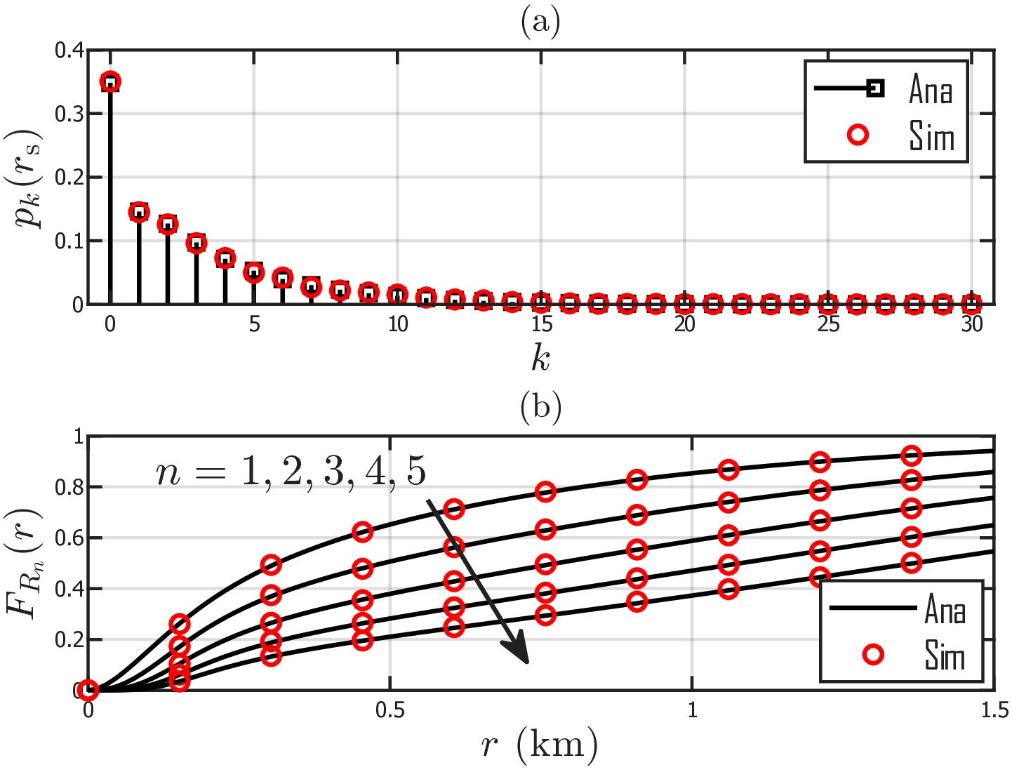
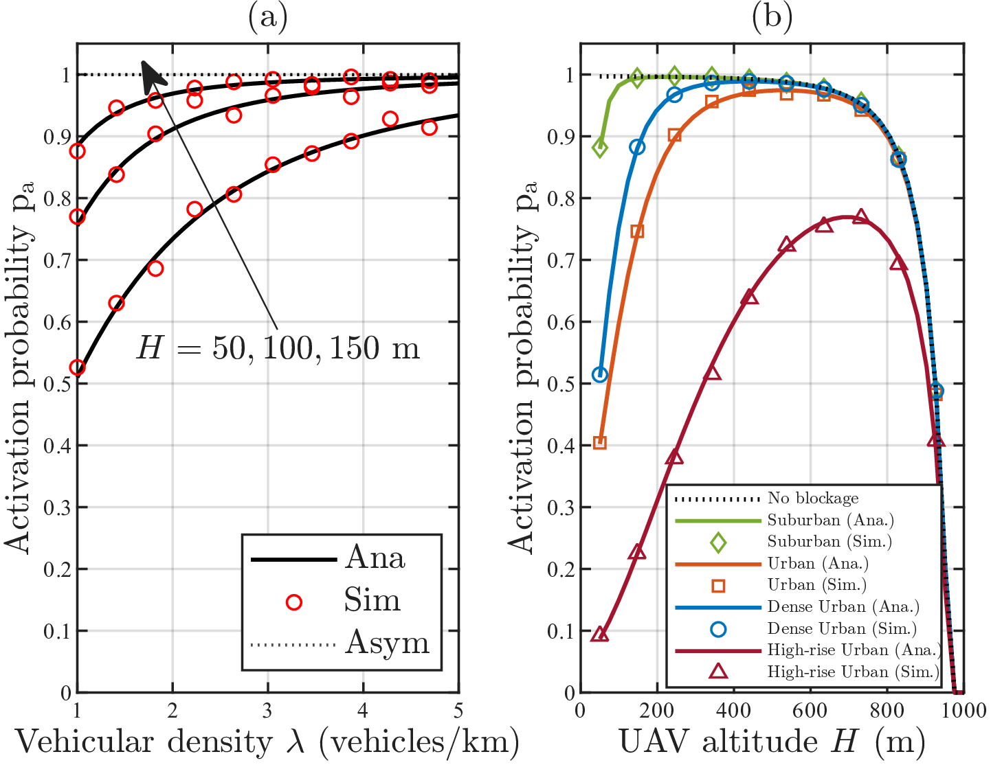
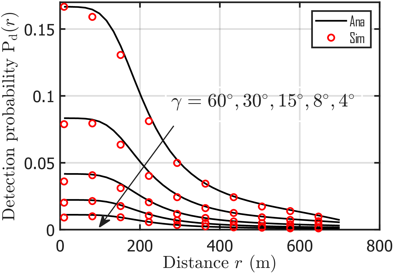
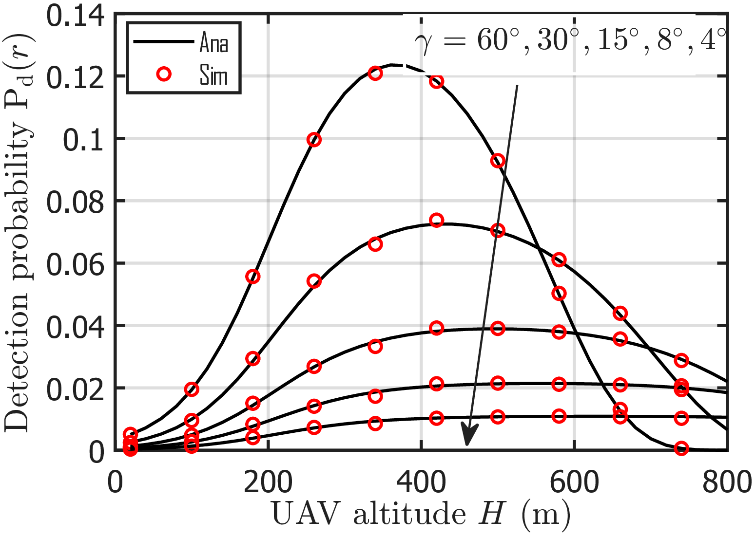
Figure 5: (a) DP \({\rm P_d}(r)\) under dense urban blockage (\(a = 9.61\), \(b = 0.16\)) versus ground distance \(r\) at fixed altitude \(H = 100\) m; (b)\({\rm P_d}(r)\) versus UAV altitude \(H\) at fixed ground distance \(r = 500\) m..
5.1 Verification of analytical results↩︎
To verify the blockage-aware distributions of the sensing load and the nearest vehicle distance, we plot the analytical and simulation results in Fig. 3. Fig. 3 (a) shows the PMF of the sensing load given in ?? . Fig. 3 (b) shows the CDF of the distance to the \(n\)th nearest LoS-detectable vehicle from the typical UAV for \(n = 1,\ldots,5\). The analytical and simulation results are in close agreement, validating the analytical framework in the presence of blockage. The high value of \(p_{\rm idle} = p_0(r_{{ \rm s}})\) in the PMF, despite the high vehicle density \(\lambda = 30~\text{vehicles/km}\), is due to both the narrow beamwidth \(\gamma = \pi/6\) and the LoS blockage at \(H = 100~\si{m}\).
5.2 Impact of altitude on activation probability↩︎
Fig. 4 (a) illustrates \({\rm p_a}\) versus the vehicular density \(\lambda\) for three UAV altitudes in a dense urban environment. As expected, \({\rm p_a}\) increases monotonically with \(\lambda\), since denser traffic raises the probability of at least one LoS-visible vehicle lying within the sensing region. For each altitude, \({\rm p_a}\) saturates toward the asymptotic limit \(1 - \exp(-4\lambda_\ell r_{ \rm s})\) as \(\lambda \to \infty\), which depends only on the road density and effective sensing radius. At a fixed \(\lambda\), \({\rm p_a}\) increases with altitude because a higher altitude steepens the elevation angle, improving \(p_{\sf L}(r, H)\) and thereby increasing the number of sensed vehicles within the sensing region. Fig. 4 (b) plots \({\rm p_a}\) as a function of UAV altitude \(H\) at \(\lambda = 1\) vehicle/km. In the absence of blockage, \({\rm p_a}\) decreases monotonically with \(H\), the growing slant distance amplifies path loss and molecular absorption, shrinking \(r_{ \rm s}^{\text{snr}}\). All four environment curves first rise, peak, and then decline. The initial rise occurs because a steeper elevation angle improves \(p_{\sf L}(r, H)\), increasing the effective density of sensed vehicle. Beyond a certain altitude, path loss and absorption dominate, and \({\rm p_{a}}\) falls. This non-monotonic behavior reveals a key design trade-off, the UAV altitude must balance LoS visibility gains against sensing range losses, yielding an environment-dependent optimal altitude that maximizes \({\rm p_a}\).
5.3 Analysis of the DP↩︎
Fig. 5 (a) plots the analytical and simulation values of DP \({\rm P_d}(r)\) with horizontal distance \(r\) for different beamwidths at a fixed altitude \(H = 100\) m. For every beamwidth, \({\rm P_d}(r)\) decays with \(r\) due to increasing path loss, molecular absorption, and diminishing LoS probability. At a given distance, a wider beam yields a higher DP. This ordering arises because the angular alignment factor \(\gamma/2\pi\) dominates the SNR gain. Fig. 5 (b) shows \({\rm P_d}(r)\) with the UAV altitude \(H\) at a fixed ground distance \(r = 500\) m. The initial rise is driven by improving LoS visibility as the elevation angle steepens with altitude, which increases the fraction of vehicles that are not blocked. Beyond a certain altitude, the growing slant distance amplifies path loss and molecular absorption, eventually dominating the LoS gain and causing \({\rm P_d}(r)\) to fall. The optimal altitude that maximises \({\rm P_d}(r)\) depends on the beamwidth. The widest beam (\(\gamma = 60^\circ\)) peaks earliest, because its moderate gain cannot sustain the SNR at large slant ranges. In contrast, the narrowest beam peaks much later, since its higher gain extends the range over which sensing remains viable, allowing it to continue benefiting from improved LoS at greater altitudes. This confirms that directionality simultaneously governs both the sensing radius, through the gain-dependent SNR, and the angular coverage, through the beam-alignment probability, establishing a fundamental trade-off whose resolution depends jointly on the target range and deployment altitude.
5.4 Sensing radius under gain–beamwidth coupling↩︎
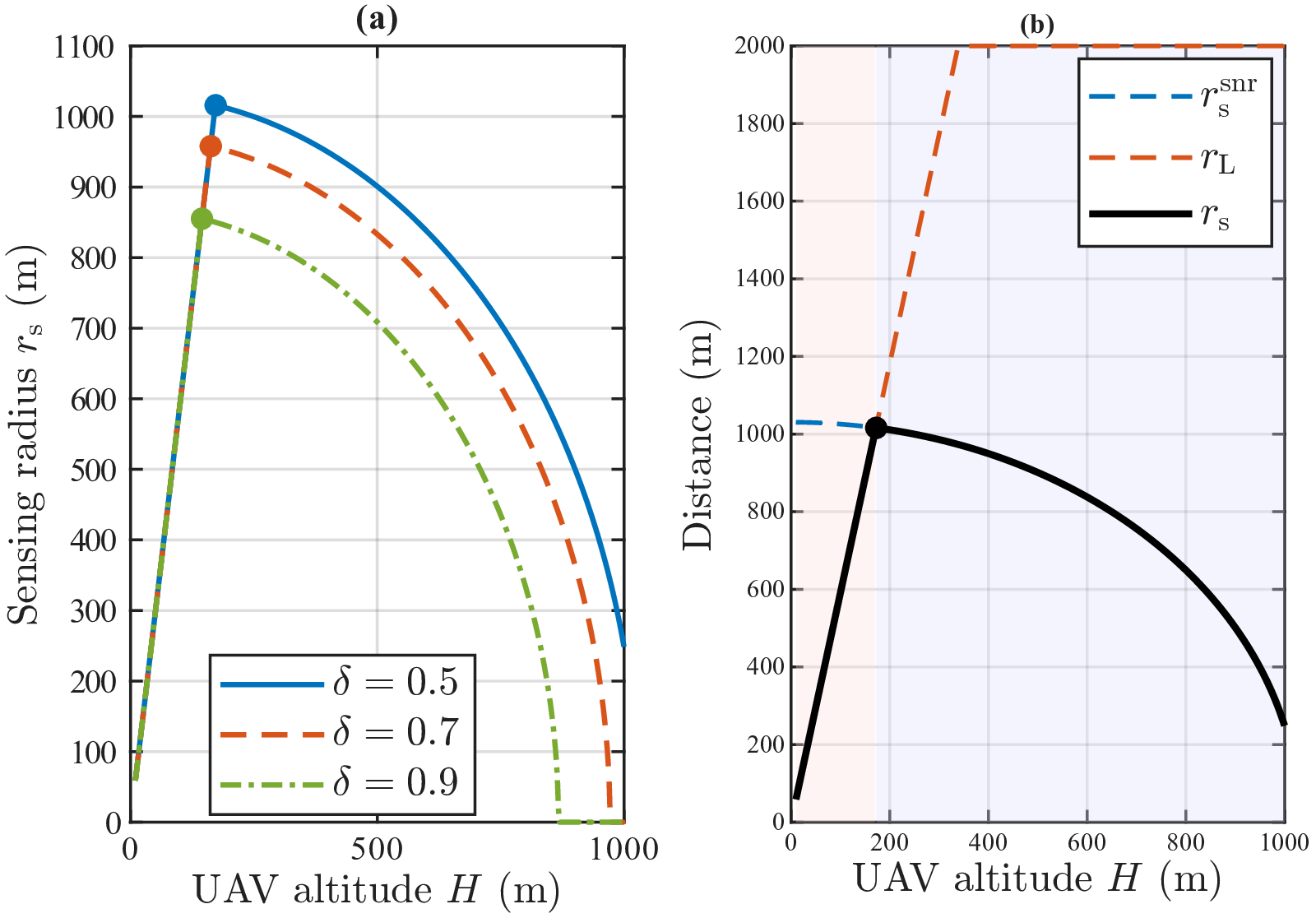
Fig. 6 (a) plots the maximum sensing radius \(r_{{ \rm s}}\) as a function of the UAV altitude \(H\) for three detection thresholds with a fixed beamwidth \(\gamma=\pi/6\). For each altitude, \(r_{{ \rm s}}\) is computed as \(\min(r_{\rm s}^{\rm snr},\,r_{\rm L})\), where \(r_{\rm s}^{\rm snr}=\sqrt{d_{{ \rm s}}^2-H^2}\) is the power-limited horizontal radius obtained from Theorem 2 and \(r_{\rm L}=H/\tan(\pi a/180)\) is the blockage-limited radius from the step-function approximation in 2 . The initial rise is driven by the improving LoS probability as the elevation angle steepens with altitude. At low altitudes, the blockage-limited radius \(r_{\rm L}\) is small because the shallow elevation angle results in frequent LoS obstruction by buildings, as \(H\) increases, \(r_{\rm L}\) grows linearly, widening the effective sensing footprint. Beyond a certain \(H\), the growing slant distance \(d=\sqrt{r^2+H^2}\) amplifies both path loss (\(d^{2\alpha}\)) and molecular absorption (\(e^{2\kappa_f d}\)), causing \(r_{\rm s}^{\rm snr}\) to shrink faster than \(r_{\rm L}\) grows, and \(r_{{ \rm s}}\) decreases. Fig. 6 (b) decomposes the sensing radius into its two limits for \(\delta=0.5\), the SNR-limited radius \(r_{\rm s}^{\rm snr}\) decreases monotonically with \(H\) as the slant distance grows, while the blockage-limited radius \(r_{\rm L}\) increases linearly with \(H\) since a higher altitude widens the LoS cone. Their minimum reveals two distinct operating regimes. At low altitudes, \(r_{\rm L}<r_{\rm s}^{\rm snr}\), placing the system in the blockage-dominant regime where the urban environment limits the sensing range regardless of the available transmit power. At higher altitudes, \(r_{\rm s}^{\rm snr}<r_{\rm L}\), and the system enters the SNR-dominant regime where signal attenuation becomes the binding constraint. The crossover between these two regimes occurs at the altitude where \(r_{\rm s}^{\rm snr}=r_{\rm L}\). This decomposition confirms that the optimal deployment altitude precisely balances LoS visibility gains against sensing range losses, and demonstrates that in the blockage-dominant regime, increasing transmit power or antenna gain yields no improvement in sensing coverage.
5.5 Interference and CP analysis:↩︎
Fig. 7 (a) presents the LT of interference at the \(k\)th nearest vehicle located at \(R_k=100\) m. As UAV altitude increases, the LoS probability improves over a wider area, raising the activation probability \({\rm p_a}\) and consequently the density of active interferers, resulting in higher resultant interference and a lower LT. Fig. 7 (b) shows that narrowing the beamwidth from \(\gamma = \pi/3\) to \(\gamma = \pi/12\) improves CP across the entire SINR threshold range. This is driven by two mechanisms: the antenna gain \(G_{ \rm s}= 2\pi/(3\gamma)\) scales inversely with \(\gamma\), strengthening the desired signal, while the angular fraction of interferers illuminating the typical UAV shrinks proportionally, reducing aggregate interference by a factor of \(\gamma/(2\pi)\). Although a narrower beam extends the sensing radius \(r_s\) via higher \(G_{\rm s}\), thereby increasing \({\rm p_a}\), this effect is outweighed by the interference reduction, yielding a net improvement in CP.
Fig. 8 (a) shows the coverage probability (CP) of the nearest sensed vehicle versus UAV altitude \(H\) for different UAV densities \(\lambda_u\). The CP decreases monotonically with altitude as signal strength decreases with increasing path loss. At low altitudes, CP across different densities remains nearly identical, but the gap widens as \(H\) increases. Although higher altitude reduces the activation probability and hence aggregate interference, the signal power degrades more severely, resulting in a net reduction in coverage. Higher UAV density further compounds this degradation through increased aggregate interference. Overall, altitude has a more dominant effect on coverage than UAV density, particularly at large \(H\).
In Fig. 8 (b), CP is compared across different propagation environments. At low altitudes, all environments achieve near-identical coverage. However, as altitude increases, suburban environments suffer the most severe degradation due to the rapid decay of signal strength with distance in open areas. In contrast, high-rise urban environments benefit from building-induced blockage of interfering links, which preserves the signal-to-interference ratio and results in a significantly slower degradation of coverage with altitude.
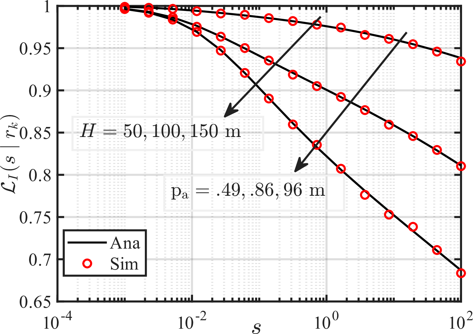

Figure 7: (a) LT of aggregate interference \(\mathcal{L}_I(s \mid r_k)\) versus \(s\) for UAV altitudes \(H \in \{50, 100, 150\}\) m, with guard distance \(r_k = 100\) m, beamwidth \(\gamma = \pi/6\), and dense urban blockage parameters (\(a = 9.61\), \(b = 0.16\)). (b) CP \({\rm p_c}^1(\tau_{\mathrm{c}})\) versus SINR threshold \(\tau_{\mathrm{c}}\) (dB) for the nearest vehicle at \(H=250\) m, with beamwidth \(\gamma\in\{\pi/12,\,\pi/6,\,\pi/3\}\). The sensing radius \(r_{ \rm s}\) follows from the reliability constraint \(\delta=0.5\), and interfering UAVs are thinned by \({\rm p_a}\)..

5.6 Analysis of the RC↩︎
Fig. 9 (a) illustrates the RC \(r_c(\tau)\) of the nearest sensed vehicle versus UAV altitude \(H\). At low altitudes, strong LoS interference dominates, while at large altitudes the signal strength deteriorates due to increased path loss. Higher UAV density consistently degrades RC through increased aggregate interference. Fig. 9 (b) shows that unlike RC, the typical RC peaks at a moderate altitude (\(H \approx 75\)–\(100\) m) and decays monotonically beyond it. At low altitudes, few vehicles fall within the sensing region (reliability threshold \(\delta = 0.2\)), limiting \({\rm p_a}\). At large altitudes, both \({\rm p_a}\) and \(r_c(\tau)\) decline simultaneously, compounding the degradation. In both panels, analytical results closely match Monte Carlo simulations, validating the derived framework. An optimal UAV altitude exists that maximizes typical rate coverage, and increasing UAV density reduces this peak.

6 Conclusion↩︎
This paper developed a tractable SG framework for sensing-assisted UAV networks serving urban vehicular communications. Roads were modeled as an MPLP, vehicles as MPLP-PPPs, and UAVs as a homogeneous 2D PPP at a fixed altitude operating under a sense-then-communicate protocol. Closed-form expressions were derived for the DP, sensing radius, sensing load distribution, UAV activation probability, CP, and RC, all validated by Monte Carlo simulations.
We observe that, at low altitude, the blockage-limited radius \(r_{\rm L}\) dominates, creating a blockage-dominant regime in which increasing transmit power or antenna gain yields no improvement in sensing coverage. At higher altitudes, the SNR-limited radius \(r_{\rm s}^{\rm snr}\) becomes the binding constraint as path loss and molecular absorption grow with the slant distance. The crossover between these two regimes is governed jointly by the UAV altitude and the urban environment parameters, establishing an environment-dependent optimal altitude that maximizes the sensing radius. The UAV activation probability exhibits a non-monotonic dependence on altitude when blockage is present, first rising as the elevation angle improves LoS visibility and then falling as path loss dominates. In high-traffic conditions, the activation probability saturates, indicating that connectivity is ultimately limited by sensing geometry, particularly road density and sensing radius, rather than vehicular density. From the communication perspective, narrower beams improve both coverage and RC by simultaneously increasing directional gain and suppressing interference through the \(\gamma/(2\pi)\) thinning factor. RC exhibits a non-monotonic behavior with altitude, while the typical RC reveals a clearly optimal deployment altitude. High-rise urban environments maintain better coverage at large altitudes due to blockage-assisted interference suppression as compare to other environment.
These results collectively establish that UAV altitude and antenna beamwidth are tightly coupled design variables that cannot be optimized independently. Efficient sensing-assisted UAV networks for urban vehicular communications require their joint design. As future extensions of this work, joint optimization of UAV altitude, beamwidth, and deployment density to maximize a unified sensing-communication utility under practical constraints is a natural next step. Incorporating UAV and vehicle mobility to study the temporal evolution of the sensing-communication trade-off and extending the framework to heterogeneous multi-tier aerial networks are further directions of interest.
7 ↩︎
Let a vehicle be located \(\mathbf{x}\equiv(r,\theta)\) with respect to the typical UAVs located at the origin. A vehicle is detected if the sensing SNR exceeds the threshold \(\tau_{ \rm s}\). Since detection requires both angular alignment and a LoS path for the radar round-trip, we condition on \(\{|\theta-{\Theta_{\mathrm{o}}}|\le \gamma/2\}\) and the LoS event, yielding \[\begin{align} {\rm P_d}(r) &= \mathbb{P}\!\left( |\theta-{\Theta_{\mathrm{o}}}|\le \gamma/2 \right)\;p_{\sf L}(r,H)\\ &\quad\times\mathbb{P}\!\left( \mathrm{SNR}_{ \rm s}(d)\ge \tau_{ \rm s} \,\big|\, |\theta-{\Theta_{\mathrm{o}}}|\le \gamma/2,\,\text{LoS} \right). \end{align}\]Because \(\theta\) is uniformly distributed over \([0,2\pi)\), the angular alignment probability is \(\mathbb{P}\!\left( |\theta-{\Theta_{\mathrm{o}}}|\le \gamma/2 \right) = \frac{\gamma}{2\pi}.\) The LoS probability \(p_{\sf L}(r,H)\) is given by 1 . Conditioned on angular alignment and LoS, the DP is \[\begin{align} \mathbb{P}\!\left( \mathrm{SNR}_{ \rm s}(r)\ge \tau_{{ \rm s}} \right) &= \mathbb{P}\!\left( \sigma \ge \frac{ \tau_{{ \rm s}} (4\pi)^3 d^{2\alpha} N_0 \exp\!\left(2\kappa_f d\right) }{ P_\mathrm{t}G_s^2(\gamma) \lambda_c^2 } \right). \end{align}\]Simplifying further completes the proof.
8 ↩︎
The sensing radius satisfies \(r_{\rm s}=\min(r_{\rm s}^{\rm snr},\,r_{\rm L})\), where \(r_{\rm L}=H/\tan(\pi a/180)\) is the blockage-limited radius from the step-function approximation 2 . Under this approximation, \(p_{\sf L}(r,H)=1\) for \(r\le r_{\rm L}\), so the conditional DP reduces to the SNR term alone \[\begin{align} {{\rm P_d^{cond}}(r)} =\exp\!\left( -\frac{ \tau_{{ \rm s}} (4\pi)^3 (d(r))^{2\alpha} N_0 \exp\!\left(2\kappa_f d(r)\right) }{ P_{\rm t}G_s^2(\gamma) \lambda_c^2 } \right). \end{align}\]The constraint \({\rm P_d^{cond}}(r)\ge\delta\) requires both the exponential SNR term and \(p_{\sf L}(r,H)\) to be sufficiently large. Considering the SNR constraint alone and imposing \({\rm P_d^{cond}}(r)\ge \delta\) yields \[\begin{align} \frac{ \tau_{ \rm s}(4\pi)^3 (d(r))^{2\alpha} N_0 \exp\!\left(2\kappa_f d(r)\right) }{ P_{\rm t}G_s^2(\gamma) \lambda_c^2 } &\le -\ln(\delta)\\ (d(r))^{2\alpha} \exp\!\left(2\kappa_f d(r)\right) &\le \frac{ -\ln(\delta)\, P_{\rm t}G_{ \rm s}^2(\gamma) \lambda_c^2 }{ \tau_{ \rm s}(4\pi)^3 N_0 }. \end{align}\]Simplifying further and applying the definition of the Lambert–\({\rm W}\) function, the power-limited maximum sensing distance \(d_{\rm s}\) is obtained as \[\begin{align} d_{\rm s}=d(r^{\rm SNR}_{\rm s}) = \frac{\alpha}{\kappa_f} \,{\rm W}\!\left( \frac{\kappa_f}{\alpha} \left( \frac{ -\ln(\delta)\, P_{\rm t}G_s^2(\gamma) \lambda_c^2 }{ \tau_{ \rm s}(4\pi)^3 N_0 } \right)^{\frac{1}{2\alpha}} \right). \end{align}\]Hence, the power-limited horizontal radius is \(r_{\rm s}^{\rm snr} = \sqrt{ d_{\rm s}^2 - H^2 }\). Combining both constraints yields \(r_{\rm s}=\min(r_{\rm s}^{\rm snr},\, r_{\rm L})\).
9 ↩︎
The typical UAV is located at the origin with its directional antenna oriented along the \(+\mathsf{x}\) direction (\(\Theta_{\mathrm{o}}=0\)). The number of detectable vehicles \(N(r)\) falling in the sensing zone of the UAV is \(N(r_{\rm s}) = N_{\rm h}(r_{\rm s}) + N_{\rm v}(r_{\rm s}),\) where \(N_{\rm h}(r_{{ \rm s}})\) and \(N_{{ \rm v}}{(r_{{ \rm s}})}\) denotes the numbers of detectable vehicles located on roads parallel and perpendicular to \(\mathsf{x}\) axis, respectively. Due to independence, the PGF of \(N(r_{{ \rm s}})\) is the product of the PGFs of \(N_{\rm h}(r_{{ \rm s}})\) and \(N_{\rm v}(r_{{ \rm s}})\). As illustrated in Fig. 10 (A), the length of the projection of the arc on the \(\mathsf{y}\) axis is \(2 r_{{ \rm s}}\sin(\gamma/2)\). Hence, the number of roads parallel to \(\mathsf{x}\) axis intersecting the sensing region is Poisson distributed with mean \(2\lambda_{\ell} r_{{ \rm s}}\sin(\gamma/2)\). On each road at distance \(\rho\), vehicles form a 1D PPP with density \(\lambda\). Since only LoS vehicles are detectable, we thin each vehicle independently with retention probability \(p_{\sf L}(\sqrt{x^2+\rho^2},H)\). The retained process is an inhomogeneous PPP with mean count \(\Lambda_{\rm h}(\rho)=\int_{\ell_{\rm h}(\rho,\gamma)}\lambda\,p_{\sf L}(\sqrt{x^2+\rho^2},H)\,\mathrm{d}x\). The PGF for the number of detectable vehicles conditioned on a road at distance \(\rho\) is \(f_{\rm h}(\rho,s) = \exp\!\big( \Lambda_{\rm h}(\rho)\,(s-1) \big)\). Conditioned on the event that exactly \(n\) roads parallel to \(\mathsf{x}\) axis intersect the sensing sector, and using the independence of different roads, the conditional PGF is \[\mathcal{P}_{N_{{\rm h}}(r_{{ \rm s}})\mid n}(s) = \left( \frac{1}{r_{{ \rm s}}\sin(\gamma/2)} \int_{0}^{r_{{ \rm s}}\sin(\gamma/2)} f_{\rm h}(\rho,s)\, \mathrm{d}\rho \right)^{n}.\]Deconditioning with respect to the Poisson-distributed number of intersecting horizontal roads yields \[\begin{align} &\mathcal{P}_{N_{\rm h}}(s) \stackrel{(a)}= \sum\nolimits_{n=0}^{\infty} \frac{e^{-2\lambda_\ell r_{{ \rm s}}\sin(\gamma/2)} \left(2\lambda_\ell r_{{ \rm s}}\sin(\gamma/2)\right)^n}{n!} \mathcal{P}_{N_{\rm h}\mid n}(s) \\ &\stackrel{(b)}= \exp\left( 2\lambda_\ell\int_{0}^{r_{{ \rm s}}\sin(\gamma/2)}\left(e^{\Lambda_{\rm h}(\rho)(s-1)} -1\right)\mathrm{d}\rho\right), \end{align}\]where \((a)\) is after deconditioning using the Poisson distribution and step \((b)\) obtained by simplifying the step \((a)\).
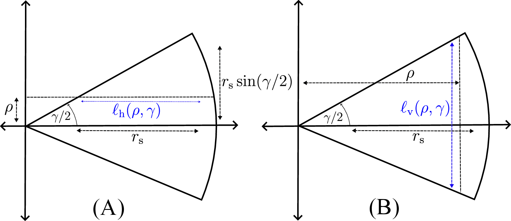
Similarly, using the Fig. 10 (B) we can determine the length of the \(\ell_{ \rm v}(\rho,\gamma)\). Then using the similar steps we can find the PGF for \(N_{{ \rm v}}(r_{{ \rm s}})\).
10 ↩︎
Using the definition LT \(\mathcal{L}_{I_k}(s)\) of \(I_{k}\) is \[\begin{align} &\stackrel{(a)}{=} \mathbb{E}_{\Phi_u^{\rm a}} \!\left[ \prod\nolimits_{\mathbf{y}\in \Phi_u^{\rm a}\setminus \mathbf{b}_{2}(\mathbf{x}_k,r_k)}\right.\notag\\ &\quad\quad\left. \mathbb{E}_{h} \!\left( \exp{\left(- s P_{\mathrm{t}} G_{\mathbf{y}} h (d(x))^{-\alpha} e^{-\kappa_f d(x)}\mathbb{1}(\text{LoS})\right)} \right) \right] \notag\\ &\stackrel{(b)}{=} \mathbb{E}_{\Phi_u^{\rm a}} \!\left[ \prod\nolimits_{\mathbf{y}\in \Phi_u^{\rm a}\setminus \mathbf{b}_{2}(\mathbf{x}_k,r_k)}\right.\nonumber\\ &\quad\left. \left(1-p_{\sf L}(x,H)\frac{ s P_{\mathrm{t}} G_{\mathbf{y}} (d(x))^{-\alpha} e^{-\kappa_f d(x)} }{ 1+ s P_{\mathrm{t}} G_{\mathbf{y}} (d(x))^{-\alpha} e^{-\kappa_f d(x)} }\right) \right] \notag\\ &\stackrel{(c)}{=} \exp\!\left( - ({\gamma\lambda_u {\rm p_a}}/{(2\pi)}) \int_{\mathbb{R}^2\setminus \mathbf{b}_{2}(\mathrm{o},r_k)} p_{\sf L}(x,H)\right.\notag\\ &\quad\quad\quad\quad\left.\times\frac{ s P_{\mathrm{t}} G_{\mathbf{y}} (d(y))^{-\alpha} e^{-\kappa_f d(y)} }{ 1+ s P_{\mathrm{t}} G_{\mathbf{y}} (d(y))^{-\alpha} e^{-\kappa_f d(y)} }\mathrm{d}\mathbf{y} \right) \notag\\ &\stackrel{(d)}{=} \exp\!\left( - \gamma \lambda_u {\rm p_{a}} \int_{r_k}^{\infty} \frac{ s P_\mathrm{t}G_{\mathbf{y}} (d(x))^{-\alpha} e^{-\kappa_f d(x)}p_{\sf L}(x,H) }{ 1+ s P_\mathrm{t}G_{\mathbf{y}} (d(x))^{-\alpha} e^{-\kappa_f d(x)} }\,x \mathrm{d}x\right)\notag \end{align}\]where step \((a)\) follows from the independence of Rayleigh fading coefficients \(\{h_{\mathbf{y}}\}\) across different UAV–vehicle links, conditioned on \(\Phi_u^{\rm a}\). Step \((b)\) is obtained by averaging the exponential fading MGF over the LoS/NLoS states. Step \((c)\) follows from the substitution \(\mathbf{y}\mapsto \mathbf{y}-\mathbf{x}_k\) and an application of the PGFL of a homogeneous PPP. Step \((d)\) is obtained by converting the resulting two-dimensional integral into polar coordinates. Simplifying further completes the proof.
11 ↩︎
The conditional CP \(\mathbb{P}(\mathrm{SINR}_k>\tau \mid R_k=r)\) is \[\begin{align} &= \mathbb{P}\!\left( h_{\mathrm{o}} > \frac{\tau (I_k+N_{0}) \left(d(r)\right)^{\alpha} e^{\kappa_f d(r)}}{P_\mathrm{t}G_\mathrm{c}} \right) \notag\\ &\stackrel{(a)}{=} \mathbb{E}_{I_k} \!\left[ \exp\!\left( -\frac{\tau (I_k+N_{0}) \left(d(r)\right)^{\alpha} e^{\kappa_f d(r)}}{P_\mathrm{t}G_\mathrm{c}} \right) \right] \notag\\ &\stackrel{(b)}{=} e^{ -\frac{\tau N_{0} \left(d(r)\right)^{\alpha} e^{\kappa_f d(r)}}{P_\mathrm{t}G_\mathrm{c}}} \mathbb{E}_{I_k} \!\left[ \exp\!\left( -\frac{\tau \left(d(r)\right)^{\alpha} e^{\kappa_f d(r)}I_k}{P_\mathrm{t}G_\mathrm{c}} \right) \right] \notag\\ &\stackrel{(c)}{=} e^{ -\frac{\tau N_{0} \left(d(r)\right)^{\alpha} e^{\kappa_f d(r)}}{P_\mathrm{t}G_\mathrm{c}}} \mathcal{L}_{I_k}\!\left( \frac{\tau \left(d(r)\right)^{\alpha} e^{\kappa_f d(r)}}{P_\mathrm{t}G_\mathrm{c}} \right), \end{align}\]where step \((a)\) is obtained using the CDF of the RV \(h_{\mathrm{o}}\), \((b)\) is obtained by separating the noise and the interference and finally \((c)\) is obtained using the LT of the interference \(I_{k}\). Deconditioning over \(R_k\) and normalizing by \(\mathbb{P}(R_k \le r_{{ \rm s}})\) yields the desired result.
12 ↩︎
The per-sector load \(L\) determines the bandwidth share \(B/L\) allocated to each vehicle. The RC must be conditioned on the event \(N(r_{\mathrm{s}})\ge 1\). Using the law of total probability over the per-sector sensing load, we write \[\begin{align} &{r}_\mathrm{c}(\tau)= \mathbb{P}\!\left( ({B}/{L})\log_2\!\left(1+\mathrm{SINR}\right) > \tau \;\middle|\; N(r_{\mathrm{s}})\ge 1 \right) \nonumber\\ &\stackrel{(a)}= \sum\nolimits_{k=1}^{\infty} \mathbb{P}\!\left(\mathcal{R}_k>\tau \mid N(r_{\mathrm{s}})=k\right)\mathbb{P}\!\left(N(r_{\mathrm{s}})=k \mid N(r_{\mathrm{s}})\ge 1\right)\notag\\ &\stackrel{(b)}=\sum\nolimits_{k=1}^{\infty}\mathbb{P}\!\left( \mathrm{SINR}_k > 2^{\frac{\tau k}{B}}-1 \right)\times ({p_k(r_{\mathrm{s}})}/{(1-p_0(r_{\mathrm{s}}))})\notag, \end{align}\]where \((a)\) is obtained by deconditioning the conditional RC and \((b)\) is obtained by simplifying the step \((a)\) and replacing the conditional load distribution as \(\mathbb{P}\!\left(N(r_{\mathrm{s}})=k \mid N(r_{\mathrm{s}})\ge 1\right) = {p_k(r_{\mathrm{s}})}/{(1-p_0(r_{\mathrm{s}}))}.\) Finally, using ?? completes the proof. Using similar steps and conditioning we can derive the RC \(r_{\mathrm{c}}^{k}(\tau)\) for the \(k\)th-nearest vehicle.
References↩︎
Kaushlendra Pandey is with the Department of Electronics and Communication Engineering, Central Institute of Technology Kokrajhar, India e-mail: (kk.pandey@cit.ac.in).↩︎
Nithin V Sabu is with the National Institute of Technology Calicut, Kozhikode, Kerala 673601, India (Email:nithinvs@nitc.ac.in).↩︎
A. K. Gupta is with Indian Institute of Technology Kanpur, Kanpur UP 208016, India (Email:gkrabhi@iitk.ac.in).↩︎