Surrogate-Gated Generation and Foundation-Model Embeddings for Bayesian Materials Design
June 26, 2026
1 Introduction↩︎
Generative models are poised to dramatically alter the way crystals with tailored properties are designed. Diffusion and flow-based models now sample crystal structures directly from a learned distribution over (near-)stable materials manifold, often conditioned on specific target properties [1], as demonstrated with CDVAE [2], DiffCSP [3], MatterGen [4], FlowMM [5], CrystalFlow [6], and the all-atom diffusion transformer ADiT [7]. Reinforcement learning sharpens these priors online by reformulating denoising as a Markov decision process. DDPO [8] and DPOK [9] first proposed to fine-tune image diffusion against a reward, and MatInvent [10] and CrystalFormer-RL [11] carry the idea to crystals. The result is a closed loop: the prior proposes, an oracle scores, and the policy updates toward higher-scoring regions of chemical space.
Whether it is density functional theory (DFT) or a machine-learning surrogate of it, scoring every proposed structure dominates the cost of the loop. A generator that emits tens of candidates per cycle quickly makes oracle calls the binding constraint. An obvious remedy is to triage: place a cheap surrogate between the generator and the oracle, and spend oracle budget only on candidates most likely to be high performing. Yet, this gating step is largely absent from closed-loop crystal generation. Surveys of generative models for materials [1] and of reinforcement-learning fine-tuning of diffusion [12] map the design space without an online, uncertainty-aware acquisition gate. The closest precedent, LCOM [13], applies a variational-autoencoder gate to crystal structure prediction, not generative design. Self-driving laboratories [14] show that surrogate-guided selection sharply reduces the number of expensive evaluations.
Such a gate can be cheap because a Bayesian-optimization surrogate [15], [16] does not need to predict property values accurately; it needs to rank candidates, as acquisition functions such as Expected Improvement are driven chiefly by how candidates are ordered relative to the incumbent best. A surrogate that puts the right structures at the top therefore remains useful even when its point predictions are poor. This relaxes the requirements on the surrogate. Foundation models for atomistic simulation, such as MACE [17], [18], ORB [19], and UMA/eSEN [20], are pretrained on millions of DFT calculations and produce transferable structural embeddings. Integration of these embeddings into a Gaussian process [21] may give exactly such a ranking surrogate with no task-specific training.
To test this end to end, we insert a Gaussian-process gate into the published MatInvent loop. The gate scores stable, novel candidates by Expected Improvement with a diversity term and sends only the top few to the oracle. We run the gated loop across three architecturally distinct pretrained priors (MatterGen, CrystalFlow, ADiT) and two property targets (room-temperature heat capacity and bulk modulus), comparing gated and ungated policies over five seeds each. The gate matches or exceeds ungated fine-tuning while capping oracle calls at a fixed per-cycle budget. A first ablation isolates the mechanism: at an identical four-call budget, ranking-based selection outperforms arbitrary selection, so the gain comes from the gate’s choice of candidates, not from spending less. A second ablation maps the efficiency frontier: in the most competitive case, the gate comes within \(\sim\)9% of exhaustive oracle spending at roughly one-fifth of the calls.
To test the same requirement outside the loop, we run a cross-factorial study over four embeddings, three Gaussian-process surrogate families, three dimensionalities, and three training-set sizes across mechanical, electronic, and vibrational property datasets (8,640 cross-validated fits). Existing benchmarks either evaluate one featurizer with one model [18] or many models on fixed descriptors [22]. In both cases they report point-prediction accuracy rather than ranking. Among the embeddings we tested, pretrained ORB with a Gaussian process was the most reliable across all three domains, and we adopt it as the default in the loop.
Section 2 formalizes the gate and the benchmark setup; Section 3 reports the closed-loop and static studies; Section 4 and Section 5 interpret the results and outline next steps.
2 Methods↩︎
2.1 Pipeline Overview↩︎
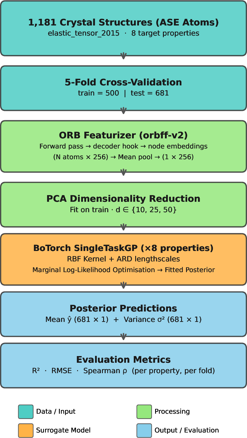
Our benchmark uses a modular pipeline with three swappable stages (Figure 1). Given a crystal structure, the pipeline proceeds as follows: (i) a featurizer converts the atomic arrangement into a fixed-length numerical vector; (ii) principal component analysis (PCA) projects this high-dimensional embedding into a reduced subspace; (iii) a probabilistic surrogate model maps the reduced features to a predictive distribution over the target property, yielding a mean prediction \(\mu(\mathbf{x})\) and uncertainty \(\sigma(\mathbf{x})\).
We evaluate three reduced dimensionalities \(d \in \{10, 25, 50\}\) via PCA [23]. PCA serves two purposes: it reduces kernel hyperparameter count (one ARD lengthscale per input dimension) and mitigates collinearity among embedding features. The PCA basis is fit on the training set only, then applied to the test set to prevent data leakage.
Any component can be swapped independently, enabling systematic cross-factorial evaluation. We tested 4 featurizers \(\times\) 3 PCA settings \(\times\) 3 surrogates \(\times\) 3 training sizes, yielding 108 configurations per dataset.
2.2 Datasets↩︎
We evaluate our pipeline on three benchmark datasets spanning material property domains: mechanical (elastic) and electronic (dielectric) datasets from the matminer library [24], and a vibrational (phonon) dataset from the Materials Project DFPT phonon database [25]. Table 1 summarizes the key characteristics of each dataset.
| Dataset | Property Type | Structures | Targets |
|---|---|---|---|
| elastic_tensor_2015 | Mechanical | \(\sim\)1,181 | 8 |
| dielectric_constant | Electronic | \(\sim\)1,056 | 4 |
| mp_dfpt_phonon | Phonon/Thermal | \(\sim\)1,253 | 4 |
Elastic tensor dataset [27] contains 1,181 inorganic crystalline structures with DFT-computed elastic constants. We predict 8 target properties: the Voigt, Voigt–Reuss–Hill (VRH), and Reuss averages of both bulk modulus (\(K\)) and shear modulus (\(G\)), together with elastic anisotropy and Poisson’s ratio. These properties range from “easy” (bulk modulus variants, depending primarily on bond stiffness and local chemistry) to “hard” (elastic anisotropy, requiring directional bonding and crystal symmetry).
Dielectric constant dataset [28] contains 1,056 structures with 4 target properties: band gap, refractive index (\(n\)), and the electronic and total components of the polycrystalline dielectric constant (poly_electronic and poly_total). These properties are sensitive to electronic structure details that are only
indirectly captured by geometric embeddings.
Phonon thermodynamics dataset is drawn from the Materials Project DFPT phonon database [25]. It contains 1,253
structures with 4 target properties evaluated at 300 K: the per-atom heat capacity (Cv_300K), vibrational entropy (S_300K), Helmholtz free energy (F_300K), and the maximum phonon frequency
(max_phonon_freq).
2.3 Featurizers↩︎
We compare four featurization strategies spanning the spectrum from classical hand-crafted descriptors to foundation model embeddings. Table 2 summarizes their key architectural differences.
| Featurizer | Type | Pretraining Data | Raw Dim. | Key Reference |
|---|---|---|---|---|
| SOAP | Classical descriptor | None (analytical) | \(\sim\)10,000+ | Bartók et al. [29] |
| MACE | Foundation model | MPTrj (\(\sim\)1.6M structs., \(\sim\)146k materials) | \(\sim\)256 | Batatia et al. [17], [18] |
| ORB | Foundation model | OMat24 (\(>\)100M configs.) | \(\sim\)256 | Orbital Materials [19] |
| UMA/eSEN | Foundation model | Multiple sources | \(\sim\)256 | Meta FAIR [20] |
SOAP (Smooth Overlap of Atomic Positions) [29] descriptors encode local atomic environments as the power spectrum of a smooth atomic density expanded in radial basis functions and spherical harmonics. We use the DScribe implementation [30] with \(r_{\text{cut}} = 5\) Å, \(n_{\max} = 4\), \(\ell_{\max} = 3\), and outer averaging. The structure-level descriptor is obtained by averaging over all atomic environments. SOAP serves as the classical baseline: it encodes only local neighborhoods within the cutoff radius.
MACE [17], [18] is an equivariant message-passing neural network that captures many-body interactions through higher-order tensor products. We extract pooled node embeddings from the pretrained MACE-MP-0 foundation model [18], which was trained on the MPTrj dataset of \(\sim\)1.6 million structures (relaxation-trajectory frames drawn from \(\sim\)146,000 Materials Project materials) [31]. We use the model as a frozen feature extractor.
ORB [19] is a graph neural network pretrained by Orbital Materials. We use the orb_v3_conservative_inf_omat checkpoint,
whose omat suffix denotes training on the OMat24 dataset of over 100 million atomic configurations. Its graph attention architecture is tuned for periodic crystal structures. We extract final-layer embeddings and average over atomic sites.
UMA/eSEN (Universal Materials Architecture) [20] is Meta FAIR’s family of interatomic potentials based on the eSCN/eSEN architecture.
Pretrained on heterogeneous materials data, UMA/eSEN is the most recently released of the foundation models we benchmark. For featurization we use the uma-s-1p1 checkpoint with the OMat task head. We extract final-layer embeddings and average
over atomic sites, as for MACE and ORB. The closed-loop probe oracle in Section 2.6 uses a separate eSEN-30M-OAM checkpoint from the same family.
2.4 Surrogate Models↩︎
All surrogate models are implemented in BoTorch [32], built on GPyTorch [33].
Gaussian Process (GP). We use BoTorch’s single-task Gaussian process at its current default: an RBF kernel with automatic relevance determination (ARD) under a dimension-scaled prior. Hyperparameters are optimized by maximizing the marginal log-likelihood. The GP is the standard surrogate for Bayesian optimization: given a set of observations, it provides a closed-form posterior over the target function with calibrated uncertainty estimates [21]. Each target property is modeled independently.
Multi-Task GP (MTGP). We use BoTorch’s multi-task Gaussian process at its current defaults: an RBF data kernel with ARD and an intrinsic coregionalization model (ICM) [34] task structure at full rank (rank = number of tasks). The ICM kernel decomposes the multi-output covariance as a Kronecker product of a task correlation matrix and a shared spatial kernel, allowing information to flow between related properties. The hypothesis is that correlated properties (e.g., \(K_{\text{Voigt}}\), \(K_{\text{VRH}}\), \(K_{\text{Reuss}}\)) should benefit from joint modeling.
Deep GP (DGP). We use a two-layer deep Gaussian process [35] built on GPyTorch’s variational deep-GP layers and wrapped with BoTorch’s multi-task model API (Matérn 5/2 hidden layer, RBF output layer with linear coregionalization), trained via variational inference [36]. The DGP stacks GP layers to capture non-linear input transformations that a single-layer GP cannot represent. However, this additional expressiveness comes at the cost of more parameters, potentially more fragile training, and sensitivity to the input dimensionality.
2.5 Experimental Protocol↩︎
For each dataset, we subsample training sets of size \(n_{\text{train}}\in \{100, 250, 500\}\) from the training fold, while the test fold remains fixed. For each \(n_{\text{train}}\) we draw a fixed training pool of size \(n_{\text{train}}\) from the dataset and route the remaining rows to a per-\(n_{\text{train}}\) held-out test set. The five evaluation runs are independent random 80/20 splits inside that training pool, all scored against the same held-out test set for the corresponding \(n_{\text{train}}\). This controls split variance while preserving a common evaluation set across configurations at a given training budget. This simulates the low-data regime typical of early-stage materials discovery, where DFT calculations are expensive.
The full factorial design yields \(4 \times 3 \times 3 \times 3 = 108\) configurations per dataset, or 324 across the three datasets. With five random splits and per-property evaluation (8 properties for elastic, 4 for dielectric, 4 for phonon), the total number of model fits is 8,640.
We report three complementary metrics:
R\(^{2}\): measures the fraction of variance explained, penalizing both bias and scatter.
RMSE (root mean square error): measures absolute prediction error in the units of the target property.
Spearman rank correlation (\(\rho\)): measures the monotonic relationship between predicted and true values; critical for Bayesian optimization, where candidate ranking matters more than exact predictions.
All metrics are computed on the held-out test set and averaged across the five random splits.
2.6 Closed-Loop Bayesian-Optimization Pipeline↩︎
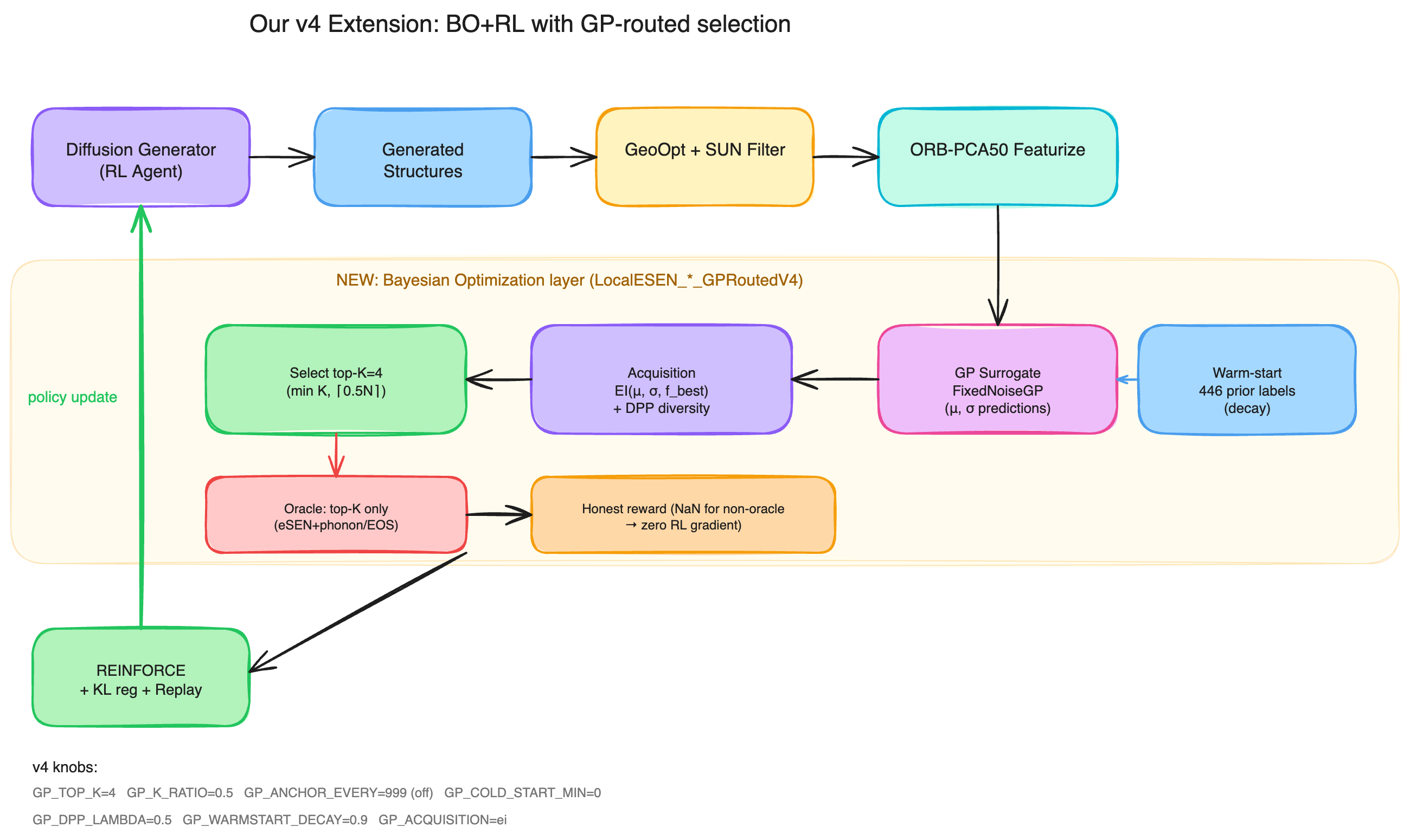
Beyond the static benchmark, we evaluate the same surrogate stack inside a closed-loop discovery pipeline that couples a pretrained generative diffusion prior to online policy-gradient updates and an uncertainty-aware acquisition gate (Section 3.1). The pipeline is a single-component modification of the published MatInvent workflow [10]: between the Stable+Unique+Novel (SUN) filter and the property oracle, we insert a Gaussian process trained on the running long-term memory and route only the top-\(K\) candidates to the oracle each cycle.
Generative backbones. We use three architecturally distinct pretrained generators that span the taxonomy of crystal generative models [1]: MatterGen [4], a joint diffusion model on atom types, fractional coordinates, and lattice parameters, trained on Materials-Project ground states; CrystalFlow [6], a graph-equivariant continuous normalizing flow with conditional flow matching; and ADiT [7], an all-atom latent diffusion transformer. Each backbone enters the loop at its publicly released checkpoint, unmodified.
Reinforcement-learning update. Following MatInvent, we treat each denoising trajectory as a stochastic policy and apply policy-gradient updates with reward-weighted Kullback–Leibler regularization against the pretrained prior: \(\mathcal{L} = \mathbb{E}_{x \sim \pi_\theta}[\,r(x) \cdot \log \pi_\theta(x)\,] + \sigma \cdot \text{KL}(\pi_\theta \,\|\, \pi_{\text{prior}})\), with \(\sigma = 0.025\). The update is supplemented by a 100-sample experience-replay buffer and a Tanimoto diversity filter (tolerance 3, buffer 6). This update rule descends directly from the DDPO [8] and DPOK [9] formulations developed for image-domain diffusion models, and is identical in BASE (ungated) and ACC (gated) except for the property calculator.
GP-gated acquisition (ACC only). Each cycle, the SUN-survivors are featurized with ORB and projected to PCA \(=\) 50 — the recommended stack from the static benchmark (Section 3.5). A single-task GP with BoTorch’s default RBF + ARD kernel is trained on the long-term memory of oracled candidates accumulated so far. We score the SUN-survivors by Expected Improvement and select the top \(K = 4\) subject to a Determinantal Point Process diversity term over the GP’s posterior mean. Only those four reach the oracle; the remaining candidates are assigned a NaN reward so they contribute zero RL gradient. Cycle 0 is
a 16-candidate warm-start: every SUN-survivor goes to the oracle so that the GP has in-loop training data before the gate begins to discriminate. In addition, the GP’s long-term memory is preloaded before cycle 0 with an externally labeled seed pool. For
\(K_{\text{VRH}}\), this is 500 structures sampled from matminer’s elastic_tensor_2015 dataset with their tabulated \(K_{\text{VRH}}\) values. For \(C_p\), it is \({\sim}446\) oracle-labeled structures pooled from earlier runs of the same pipeline. These preloaded points (tagged cycle \(-1\)) are
down-weighted in the GP fit by an age-dependent noise inflation but remain in the training set throughout, so the GP never operates from a 16-point cold start. The per-run oracle budgets reported in Section 3.1 count in-loop oracle calls only. The same seed pool is the reference set for the novelty analysis (Section 3.1.8).
Property oracle. The oracle is itself a learned surrogate of DFT. For heat capacity at room temperature (\(C_p\)), we relax each candidate with the eSEN-30M-OAM machine-learning interatomic
potential [20] and feed the relaxed structure into phonopy [37] for a quasi-harmonic phonon calculation that yields \(C_p(T = 300\,\text{K})\) (distinct from the static-benchmark phonon target Cv_300K of Section 2.2, which is a DFPT per-atom heat capacity). For the Voigt–Reuss–Hill bulk modulus (\(K_{\text{VRH}}\)), we compute energies under seven uniform strains in the range \(\pm 3\%\) with eSEN-30M-OAM and fit a Birch–Murnaghan equation of state [38]. Beyond this learned oracle, we
recompute the bulk modulus of the top candidates with DFT as an oracle-parity check (Section 2.7); the corresponding heat-capacity validation is substantially more costly and is left to future work.
Run protocol. Each closed-loop trajectory runs for 20 RL cycles with a per-cycle design budget of up to 16 candidates after SUN filtering; the realized count varies by backbone (MatterGen approaches the budget; CrystalFlow and ADiT typically deliver \(\sim\)5–10 SUN-survivors per cycle). We run five random seeds for each \(\{\)backbone, target, policy\(\}\) cell, giving 30 trajectories per target (\(C_p\) and \(K_{\text{VRH}}\)); one ADiT/ACC \(C_p\) seed did not complete, leaving 29 on \(C_p\) and 30 on \(K_{\text{VRH}}\). Per-seed running-best property values are forward-filled to the full 20-cycle horizon before averaging across seeds, so the cross-seed mean is itself non-decreasing; this is the cross-seed equivalent of the standard convention used by MatInvent’s own discovery curves. Concurrent benchmark frameworks for closed-loop materials discovery [39] and for cross-model evaluation of crystal generators [40] provide complementary protocols; the present pipeline reports a specific gating method run end-to-end across three pretrained priors.
2.7 DFT Validation of Generated Structures↩︎
To anchor the closed-loop probe’s learned oracle and surrogate to first-principles ground truth, we recompute the bulk modulus of the top generated \(K_{\text{VRH}}\) structures with DFT and replay the GP surrogate causally against those values (Section 3.1.10). We validate the bulk-modulus target only: its oracle is a seven-point equation-of-state fit (seven single-point energies per structure), whereas the heat-capacity oracle requires a phonon supercell with tens to over a hundred displacement calculations on 40–580-atom cells, roughly an order of magnitude more expensive; a DFT check of the heat-capacity target is therefore left to future work.
Oracle-parity equation of state. The DFT bulk moduli are computed to be like-for-like with the eSEN oracle, so that the comparison isolates the oracle’s error rather than a generic DFT-versus-MLIP gap. Each generated cell is first refined to its nearest space group with spglib [41] so that VASP [42] can exploit the symmetry. Cells for which spglib finds no symmetry above the tolerance are computed without symmetry (space group P1). The cell and ions are then relaxed under Materials-Project-compatible settings [43]—the PBE functional [44], projector augmented-wave potentials [45], [46], a 680 eV plane-wave cutoff, and spin polarization, with no Hubbard \(U\) correction, as none of the validated chemistries falls under the Materials Project \(+U\) scheme [26]. From the relaxed cell we apply seven rigid isotropic strains \(\varepsilon \in \{-3\%, \dots, +3\%\}\) with frozen fractional coordinates and a single static calculation at each—mirroring the oracle, which likewise does not relax ions at strained volumes—and fit a third-order Birch–Murnaghan equation of state [38] to obtain \(K_0\). A single \(k\)-point grid, fixed from the relaxed reference (reciprocal spacing \(0.16\) Å\(^{-1}\)), is used for all seven strains, since regenerating the mesh per strained cell perturbs the curvature of the fit; the statics use the tetrahedron method with an energy threshold of \(10^{-7}\) eV. Every validated structure yields an in-window fit with a physical pressure derivative \(B_0' \in [4.1, 5.1]\).
Causal surrogate replay. Because the validated structures are members of the closed-loop long-term memory, training the GP on the full memory and then predicting them would measure memorization rather than generalization. We instead replay each ACC run causally: stepping through cycles in order, at cycle \(s\) we train the GP on all structures gathered before cycle \(s\)—including the preloaded warm-start seed pool (Section 2.6)—and predict the freshly generated cycle-\(s\) candidates, which the surrogate has not yet seen. The analysis is restricted to the ACC runs, the only ones that employ a GP gate.
2.8 Synthesizability Scoring of Generated Structures↩︎
We assess the synthesizability of generated structures with two independent composition-level models and compare them. The first is an ORB-based positive-unlabeled classifier (ORB-PU) trained here; the second is the pretrained composition-graph model of Jang et al. [47] (CGNF).
Training data. We assemble 109,283 Materials Project compositions: 49,283 entries whose Materials Project records carry an ICSD cross-reference (experimentally synthesized) as labeled positives, and 60,000 theoretical entries with no ICSD cross-reference and energy above hull below 0.5 eV/atom as unlabeled, split into train, validation, and test (76,498 / 10,928 / 21,857) stratified by label. Holding out known positives and treating the unlabeled pool as pseudo-negatives matches the evaluation protocol used by CGNF.
Features and classifier. Each composition is represented by its mean-pooled ORB embedding reduced with the benchmark PCA (Section [sec:pca]), concatenated with Magpie descriptors [48]; an ORB-energy stability scalar is an optional third block. The classifier is a Mordelet–Vert positive-unlabeled bagging ensemble [49]: each bag keeps all positives and draws a random subsample of the unlabeled pool as pseudo-negatives, sized by a tuned multiple of the positive count and capped at the pool size, and per-bag positive probabilities are averaged. In the selected configuration (19 bags, negative-sampling ratio 1.29) the cap binds, so every bag trains on the full unlabeled pool and ensemble diversity comes from the base learner’s per-bag random seed and column subsampling rather than from the unlabeled draw. An abstention layer marks a composition as out-of-distribution when its standardized nearest-neighbor distance to the positive training set exceeds the 95th percentile of that distance among positives, or when bag disagreement or prediction confidence fall outside fixed thresholds.
Hyperparameter tuning. Hyperparameters are tuned with Optuna [50] (tree-structured Parzen sampler, median pruner, five-fold stratified cross-validation) to maximize the area under the precision–recall curve on the held-out positive-versus-unlabeled split, over feature sets {Magpie, ORB, ORB+Magpie, ORB+Magpie+stability} and base learners {random forest, gradient-boosted trees}; the bag count and negative-sampling ratio are tuned jointly with each learner’s hyperparameters. The selected model is ORB+Magpie with gradient-boosted trees (Supplementary Table S4).
Evaluation. On the held-out Materials Project test split the selected ORB-PU model and pretrained CGNF are scored on the same compositions (Supplementary Table S5); these numbers favor ORB-PU because it is in-distribution whereas CGNF is applied zero-shot, so we do not read them as a method-superiority comparison. The comparison on equal footing is on the generated structures (Section 3.1.9), where both models are out-of-distribution.
3 Results↩︎
We first consider a closed discovery loop, wrapping three pretrained diffusion priors with an online policy-gradient update and a Gaussian-process acquisition gate, and ask whether the gate improves on ungated fine-tuning (Sections 3.1–3.1.5). We then test the principle behind the gate’s low cost (a Bayesian-optimization surrogate need only rank candidates, not predict their values) in a static cross-factorial benchmark of embeddings and surrogates across mechanical, electronic, and vibrational properties (Section 3.2).
3.1 Closed-Loop Probe with Diffusion Backbones↩︎
The static benchmark indicates that an ORB + GP surrogate should remain useful in closed-loop Bayesian optimization (BO). We tested this with three architecturally distinct pretrained diffusion priors, fine-tuned online via the policy-gradient procedure of MatInvent [10], with a Gaussian Process surrogate inserted between the SUN-filter and the property oracle. The reinforcement-learning side of the procedure follows the lineage of DDPO [8] and DPOK [9] from the image domain, ported to crystals by MatInvent and (concurrently, for an autoregressive transformer prior) by CrystalFormer-RL [11]. Existing tutorials and reviews of RL fine-tuning of diffusion models [12] catalog several policy-gradient and value-based families, none of which include a Bayesian-optimization gate at acquisition time. A recent review of generative AI for crystals [1] likewise surveys the design space without devoting a section to closed-loop, online surrogate-gated refinement, although it notes one offline precedent: Qi et al.’s Latent Conservative Objective Models (LCOM) [13], which trains a conservative surrogate over a CDVAE latent space to minimize formation energy. LCOM differs from the present work in being offline (no online policy update of the generator), single-property (formation energy), and built around a CDVAE rather than a diffusion prior; we view it as a complementary precedent rather than a baseline. The probe in this section sits in that gap.
We ran two property targets (\(C_p\) and \(K_{\text{VRH}}\)), two policies (BASE and ACC, defined below), three backbones, and five seeds, giving 29 completed \(C_p\) runs and 30 \(K_{\text{VRH}}\) runs. The diffusion priors are not retrained from scratch; they are updated only through online REINFORCE-style rollouts. The oracle is itself a learned surrogate (eSEN-30M-OAM [20] fed into phonopy [37] for \(C_p\) and a Birch–Murnaghan fit [38] for \(K_{\text{VRH}}\)); the bulk-modulus candidates are subsequently validated against DFT (Section 3.1.10), while the heat-capacity candidates are not DFT-validated here. With those caveats noted, the runs are large enough to examine cross-backbone behavior, characterize the GP surrogate as the loop progresses, and report the practical effect of inserting the gate into a published RL pipeline.
3.1.1 Pipeline and Setup↩︎
The three backbones are MatterGen [4], CrystalFlow [6], and ADiT [7]. Each runs under two policies. BASE follows the published MatInvent recipe [10] verbatim: policy-gradient updates with reward-weighted KL regularization against the pretrained prior (\(\sigma = 0.025\)), an experience-replay buffer (size 100, sample size 10, reward cutoff 0.1), and a diversity filter on the long-term memory (tolerance 3, buffer 6). ACC differs from BASE only in the property calculator: between the SUN filter and the oracle it inserts a Gaussian Process surrogate over ORB + PCA50 features, scores SUN-survivors by the acquisition rule (Expected Improvement plus a Determinantal Point Process diversity term), and dispatches only the top \(K = 4\) to the oracle each cycle; the remaining candidates receive NaN reward, so they do not contribute to the policy-gradient update. Every other RL hyperparameter (KL coefficient, replay buffer, diversity filter, finetune epochs, batch size \(\sim 16\) candidates per cycle) is identical between BASE and ACC. Each run lasts 20 cycles, and every candidate must pass the Stable+Unique+Novel (SUN) screen before any oracle or surrogate call.
3.1.2 Discovery Curves Across Backbones↩︎
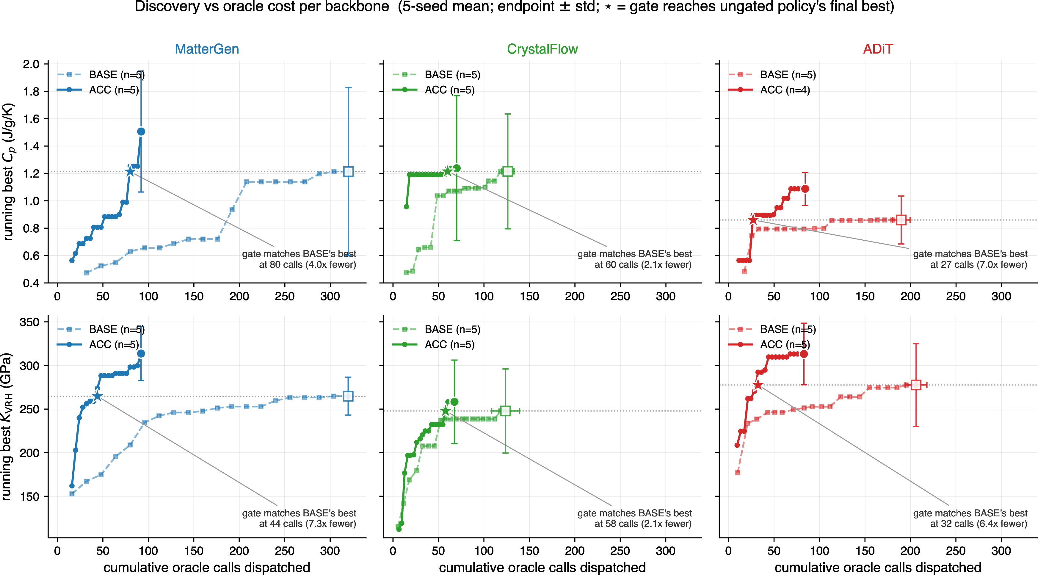
Figure 3 plots the running best oracled property against cumulative oracle calls, one panel per backbone; per-seed running-bests are forward-filled to the full cycle horizon before averaging, so the cross-seed mean is itself non-decreasing. This view pairs discovery with its cost: a curve that rises further up and left finds better materials on a smaller oracle budget. For \(C_p\), the gated policy ends at seed-mean running bests of 1.51 (MatterGen), 1.24 (CrystalFlow), and 1.09 J/g/K (ADiT), above BASE in every backbone. For \(K_{\text{VRH}}\), MatterGen and ADiT plateau near 310 GPa under ACC; the single best structure (375 GPa) is an MoN polymorph in space group \(P\,\bar{6}m2\) (#187) found by ADiT/ACC at seed 7. The starred markers locate where the gate first matches the ungated policy’s end-of-run best: at 2.1–7.3\(\times\) fewer oracle calls in all six (backbone, target) cells. CrystalFlow shows the largest between-seed spread of the three backbones for both targets, so its mean comparison is the noisiest of the panel, but the ACC mean still sits above the BASE mean throughout. The qualitative pattern is consistent with the static benchmark, which is discussed in detail later in the text and supplementary information: the ORB + GP surrogate ranks candidates well enough to drive acquisition without breaking the underlying RL update. Direct numeric comparison with the published MatInvent heat-capacity run (Fig. 2c of [10]) is limited because the two curves plot different quantities: their 10-seed mean tracks the per-loop average \(C_p\) of generated structures, reaching \({\approx}0.6\) J/g/K at loop 20 on its way to the 1.5 J/g/K target near loop 60, whereas our curves track the running best. At a matched 20-loop budget the two setups are nonetheless in a similar regime: their loop-20 batch mean sits below our 5-seed BASE running-best mean of \(1.2 \pm 0.6\) J/g/K, as a batch-mean versus best-so-far statistic must.
3.1.3 Surrogate Quality Across Cycles↩︎
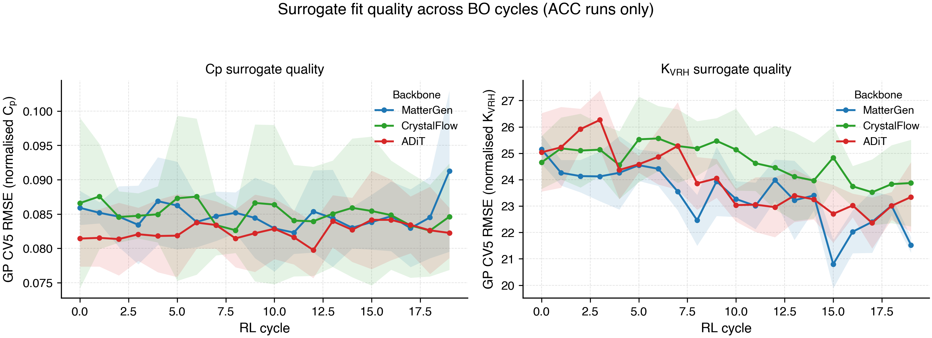
Figure 4 plots the GP CV5 RMSE per cycle, ACC runs only. This metric is 5-fold cross-validation on the GP’s full training set at that cycle: the pre-loaded labeled seed pool described in Methods, plus the oracled warm-start candidates and all top-\(K\) acquisitions up to the current cycle (\({\sim}450\) points at cycle 0 growing to \({\sim}510\) by cycle 19 on \(C_p\); \({\sim}510\) growing to \({\sim}590\) on \(K_{\text{VRH}}\)). It measures how well the GP fits its own oracled labels under leave-one-fold-out resampling; it does not measure error on the next batch of fresh diffusion proposals, the candidates the gate actually scores with the GP posterior mean \(\mu\). On \(C_p\) the CV5 RMSE sits at 0.080–0.091 (normalized property scale) and is statistically flat across cycles: mean RMSE in cycles 0–5 differs from cycles 15–19 by less than one between-seed standard deviation. \(K_{\text{VRH}}\) shows the same pattern at the 21–26 GPa level, with a mild downward trend in MatterGen and CrystalFlow. The GP thus remains well-fitted to training data as the training set grows, a necessary but not sufficient condition for surrogate-gated BO health. A held-out RMSE on the diffusion proposals before they reach the gate is not in our current logs; for the bulk-modulus target, however, the causal surrogate replay of Section 3.1.10 measures generalization directly as a ranking on those fresh proposals (Spearman \(\rho = 0.944\)).
3.1.4 Oracle-Call Savings from the GP Gate↩︎
The GP gate’s practical benefit is that it caps the number of expensive oracle calls per cycle at \(K=4\) regardless of how many candidates pass the SUN filter, replacing the rest with cheap GP-\(\mu\) pseudo-evaluations. Supplementary Fig. S2 compares the per-cycle schedules of cumulative oracle calls between BASE (every SUN-survivor goes to the oracle) and ACC (top-\(K=4\) only) for both targets. ACC’s curve is the same straight line for every backbone: 16 oracle calls for the warm-start at cycle 0, then 4 per cycle, totaling 92 calls per 20-cycle run. BASE’s curve depends on each backbone’s SUN-survival rate.
Total oracle calls per run, 5-seed mean: for \(C_p\), BASE/ACC is 320/92 in MatterGen (\(3.48\times\) saving), 126/70 in CrystalFlow (\(1.80\times\)), and 190/84 in ADiT (\(2.25\times\)); for \(K_{\text{VRH}}\), BASE/ACC is 320/92 in MatterGen (\(3.47\times\)), 124/68 in CrystalFlow (\(1.83\times\)), and 206/83 in ADiT (\(2.49\times\)). The pattern is consistent: SUN survival per cycle exceeds \(K=4\) in every (backbone, target) cell, with roughly 6–16 candidates dispatched per cycle, so the gate reduces the oracle-call count throughout, by the largest factor for MatterGen, where survival is highest. Beyond the call count, the gate also changes which candidates are scored: it forces a top-\(K\) selection by EI + DPP rather than letting whatever survives the SUN filter pass through to the oracle, an effect the budget-matched ablation isolates next. Measured at matched quality rather than matched cycles, the same data give a sharper statement: the gate first reaches BASE’s end-of-run best with \(2.1\)–\(7.3\times\) fewer oracle calls in all six (backbone, target) cells (stars in Figure 3).
3.1.5 Budget-matched ablations: candidate selection versus call count↩︎
The gate changes two things at once relative to vanilla REINFORCE (BASE): it spends fewer oracle calls, and it chooses which candidates to spend them on. To separate these effects we ran two MatterGen controls that hold the generation front-end fixed (64 proposals per cycle, identical SUN filter) and vary only the back-end selection (Figure 5).
The first control, cap-4, matches ACC’s oracle budget exactly (four oracle calls per cycle) but selects the four arbitrarily, taking the first four survivors of the SUN filter rather than ranking them by Expected Improvement. If the gate’s benefit were the reduced call count alone, cap-4 would track ACC. It does not: by cycle 20 cap-4 reaches only \(0.86 \pm 0.58\) J/g/K on \(C_p\) and \(233 \pm 30\) GPa on \(K_{\text{VRH}}\), against ACC’s \(1.51 \pm 0.44\) J/g/K and \(314 \pm 31\) GPa. At an identical budget, it is the surrogate’s choice of which four candidates to evaluate, not the reduced call count, that drives discovery.
The second control, oracle-all, removes the budget cap and sends every SUN survivor to the oracle (roughly 25 per cycle for MatterGen on \(K_{\text{VRH}}\)), giving the brute-force ceiling at \(\sim\)442 oracle calls per run against ACC’s 92. It reaches \(341 \pm 30\) GPa on \(K_{\text{VRH}}\), about 9% above ACC at \(4.8\times\) the oracle cost. The gated policy therefore comes within a tenth of exhaustive spending figure of merit while paying roughly a fifth of the budget. On \(C_p\) the SUN cap never binds for MatterGen, so oracle-all coincides with BASE and is plotted as such.
Two of the five cap-4 \(C_p\) seeds initially terminated early, on cycles where all four oracle calls returned no valid reward and the policy gradient had nothing to update against; both were re-run to completion, and the re-runs enter the five-seed aggregate. An overly tight oracle budget can thus starve the loop, a failure mode the gate avoids by spending its four calls on the most promising survivors rather than on whatever the filter happens to emit first.

3.1.6 Crystal-System Distribution of Generated Top Structures↩︎
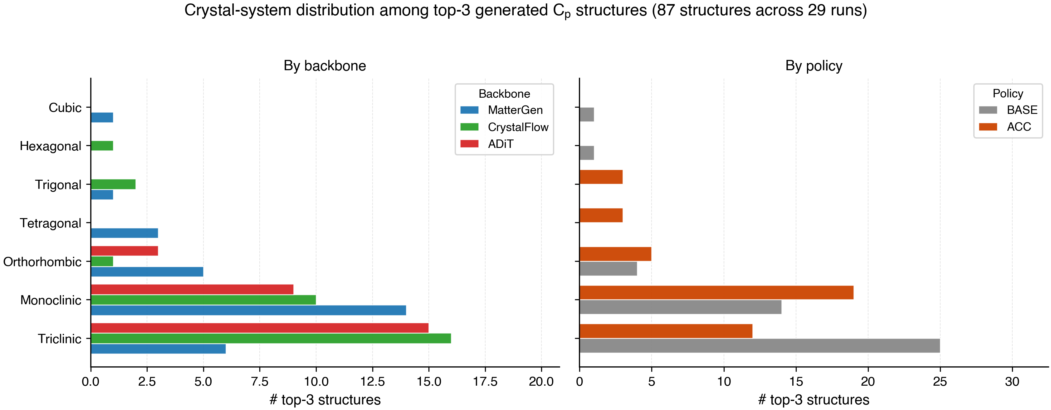
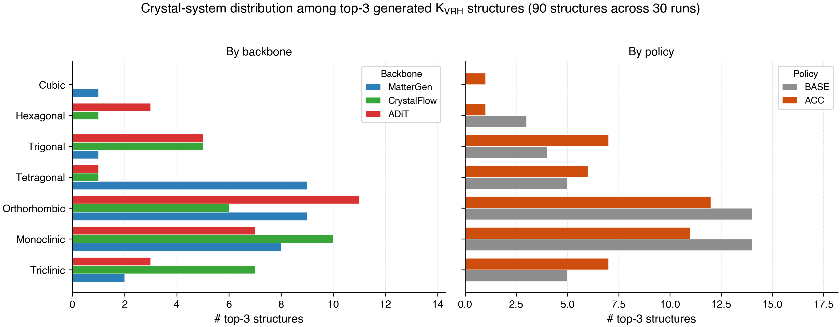
The space groups of the top-3 candidates per run reveal a strong asymmetry across backbones (Figure 6). For \(C_p\), CrystalFlow and ADiT both produce more than half of their top structures in triclinic and monoclinic systems, the lowest-symmetry crystal classes, while MatterGen splits more evenly, contributing the bulk of the orthorhombic and tetragonal hits. All three priors are trained on Materials-Project-derived data (MatterGen on Alex-MP-20; CrystalFlow and ADiT on MP-20), so this spread reflects differences in model architecture and online fine-tuning rather than in training set. We report it as an empirical observation. For \(K_{\text{VRH}}\) (Figure 7) the dominance of low-symmetry systems persists, but cubic and hexagonal structures are over-represented relative to \(C_p\), reflecting the well-known correlation between high bulk modulus and densely packed cubic/hexagonal lattices. Splitting by policy (right panel) shows that the GP gate (ACC) does not bias the loop towards any particular crystal system: both BASE and ACC produce the same broad triclinic/monoclinic dominance, so the GP is screening on the property rather than on geometric proxies.
3.1.7 Per-Backbone Summary↩︎
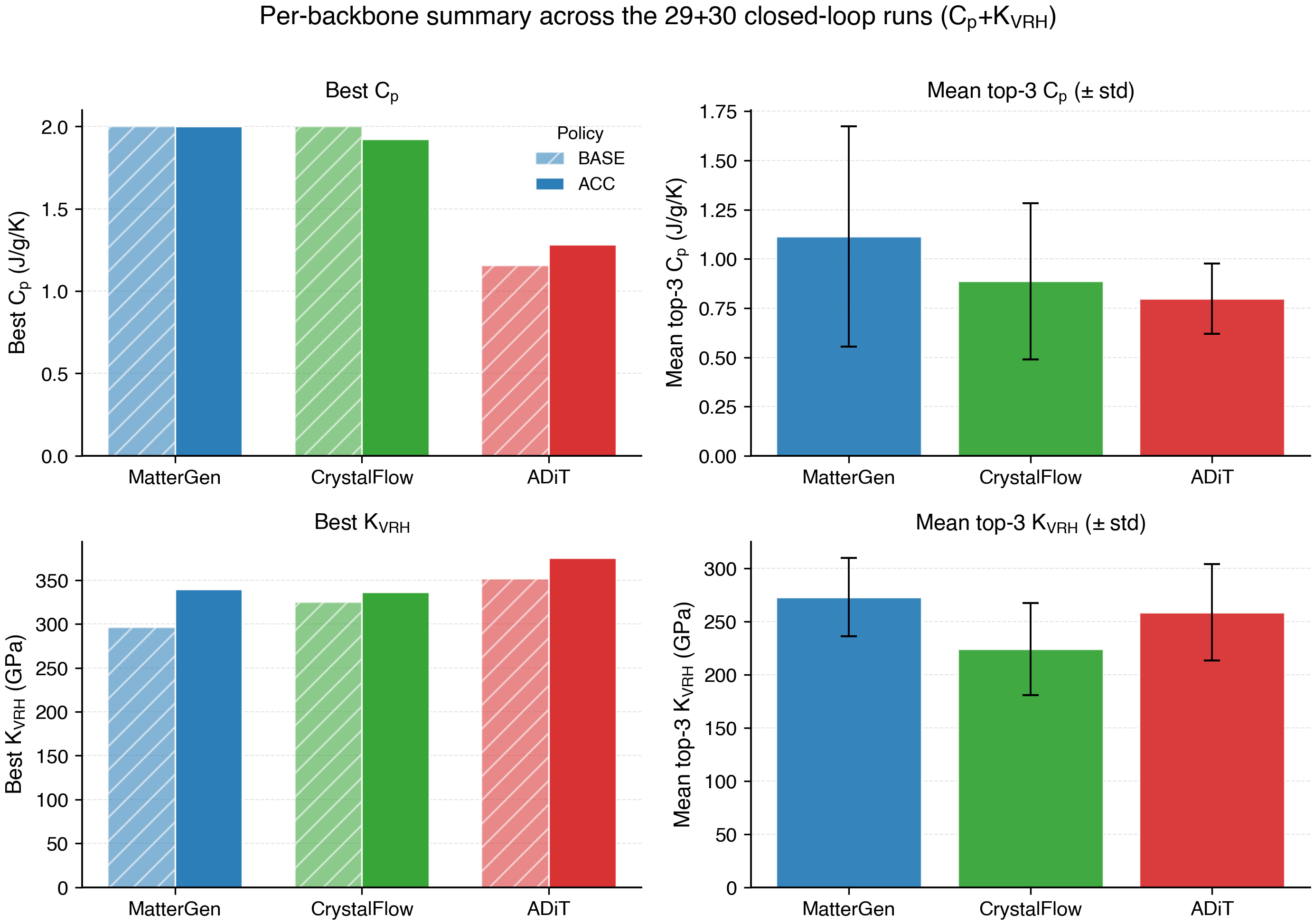
Figure 8 consolidates the summary statistics per backbone across all completed runs (29 \(C_p\), 30 \(K_{\text{VRH}}\)). Best-value bars (left column) split BASE vs.ACC: MatterGen and CrystalFlow both hit the 2.0 J/g/K reward ceiling (oracle-imposed cap, attained on a few seeds) while ADiT plateaus at 1.28 J/g/K; for \(K_{\text{VRH}}\), ADiT’s 375 GPa hit pulls its best-value bar above MatterGen’s 340 and CrystalFlow’s 336 GPa. Mean top-3 (right column) is the more robust comparator, since best-of-run is dominated by favorable seeds: on \(C_p\) the three backbones land at 1.11 \(\pm\) 0.56, 0.89 \(\pm\) 0.40, and 0.80 \(\pm\) 0.18 J/g/K, differences smaller than the within-backbone seed spread. On \(K_{\text{VRH}}\) the corresponding means are 273 \(\pm\) 37, 224 \(\pm\) 43, and 259 \(\pm\) 45 GPa, again with overlapping error bars. Novelty against the warm-start seed pool is uniform across backbones at 100% for \(C_p\) and 96.7% for \(K_{\text{VRH}}\), so we report it verbally rather than as a separate panel; details and the formula-level analysis are in Section 3.1.8. The ACC-vs-BASE lift on best-of-run is consistent in MatterGen and ADiT (Section 3.1.2) but never large enough to outweigh seed variance, so we report it as a trend rather than a measured difference.
3.1.8 Novelty vs.the Warm-Start Seed Pool↩︎
A natural concern is that the loop is retrieving the structures we used to warm-start the GP rather than producing new ones. We checked this with pymatgen’s structure matcher [43] at default tolerances. For \(C_p\), none of the 87 top-3 structures (aggregated across the 29 completed runs) shares a reduced formula with the seed pool, and zero pass strict matching. For \(K_{\text{VRH}}\), 3 of 90 share a reduced formula but again zero pass strict matching. The GP is acting as a property prior, not as memory.
Figure 9 shows the top-20 structures per target, borders coded by backbone. The compositions split along physical lines: light-element binaries and ternaries (Li, Mg, Na, O) for \(C_p\), transition-metal carbides, nitrides, and borides (Mo, W, Os, Re) for \(K_{\text{VRH}}\), roughly what each property’s known physical drivers would predict.
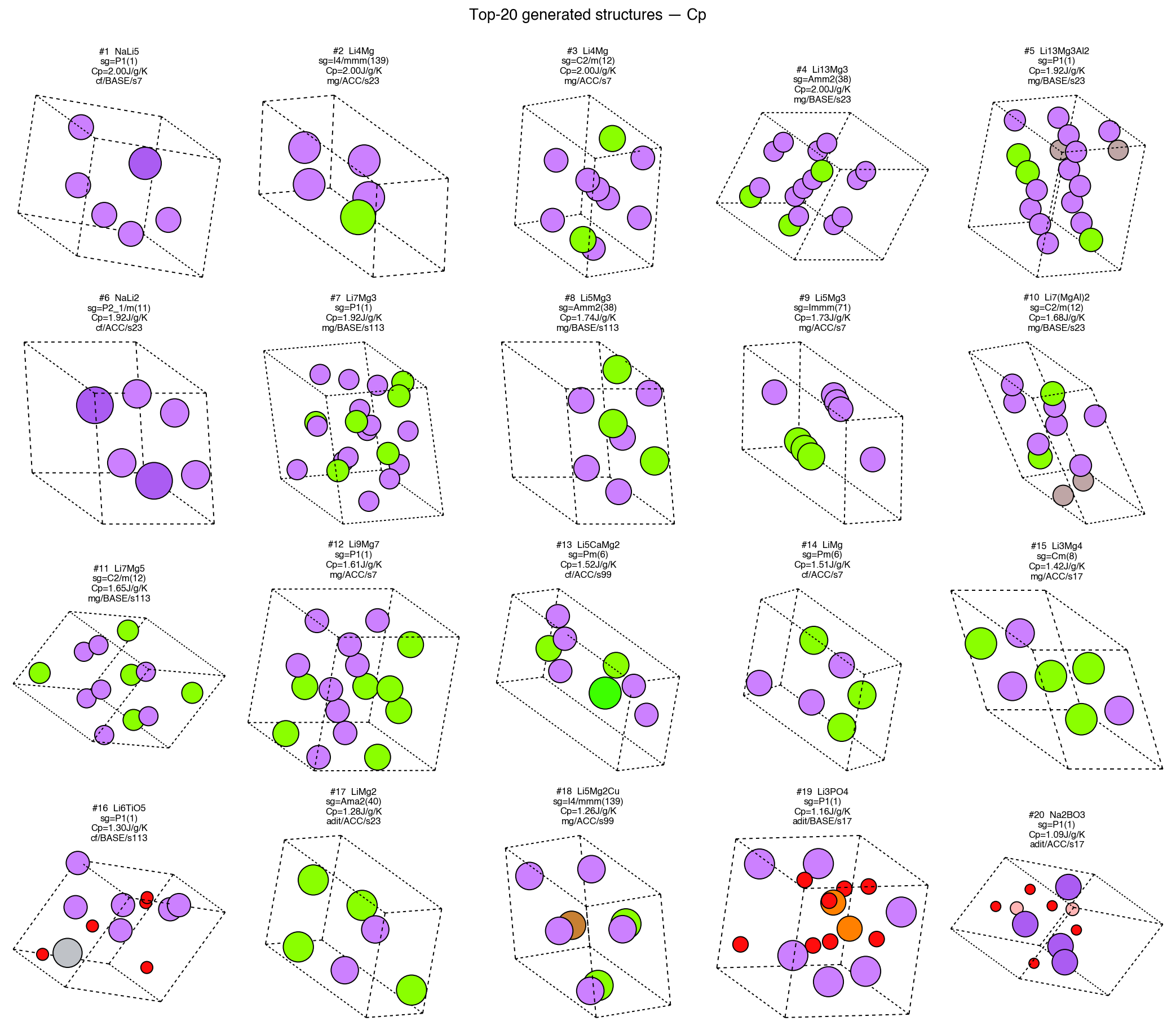
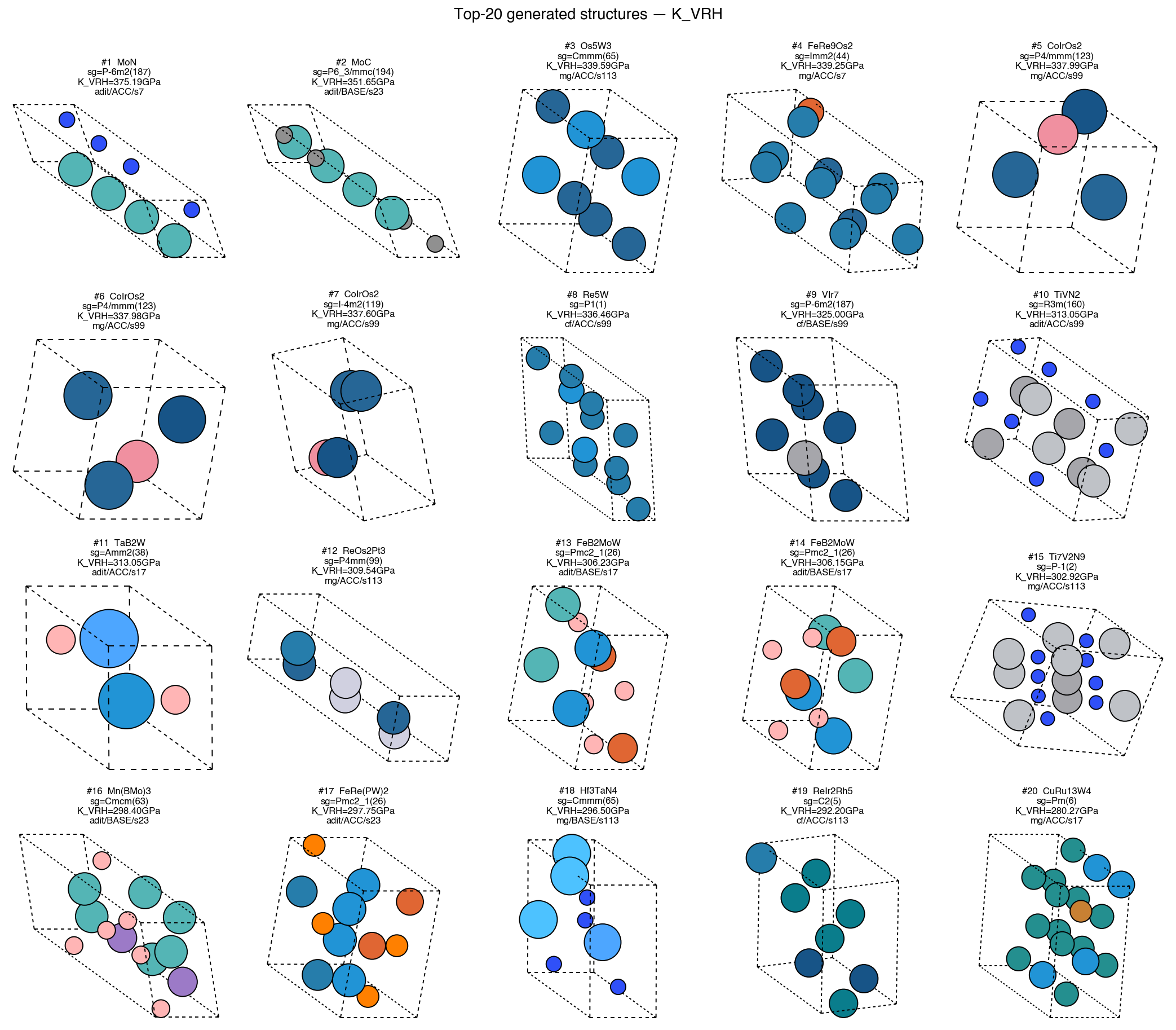
Figure 9: Top-20 generated structures per target (4\(\times\)5 grid), ranked by the oracle. Border color: blue = MatterGen, green = CrystalFlow, red = ADiT. Each panel reports formula, space group, target value, and the originating (cycle, seed). None pass strict structure matching against the warm-start seed pool.. a — Heat capacity (\(C_p\)), b — Bulk modulus (\(K_{\text{VRH}}\))
3.1.9 Synthesizability of Generated Structures↩︎
We score the top generated structures for synthesizability with two independent composition-level models (Section 2.8): an ORB-based positive-unlabeled classifier (ORB-PU) trained here, and the pretrained CGNF model [47]. Neither model saw these structures in training, so this is a comparison of two scorers on equal, out-of-distribution footing, unlike the in-distribution test-split numbers in Supplementary Section S6.
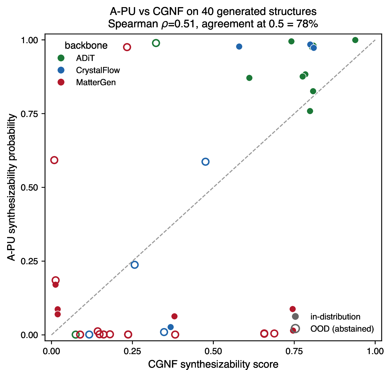
Across the 40 top structures the two scores agree moderately: Spearman \(\rho = 0.51\) and 78% agreement at the conventional 0.5 decision threshold (Figure 10). They concur on conventional main-group chemistries, for example Na\(_2\)BO\(_3\), Li\(_3\)PO\(_4\), and TaB\(_2\)W, and diverge on lithium–magnesium binaries and several heavy intermetallics, where ORB-PU assigns low probabilities and flags out-of-distribution.
The ORB-PU out-of-distribution criterion flags 21 of 40 structures (52.5%), almost all by distance rather than low confidence or bag disagreement. The flagged fraction varies by backbone (Figure 11): it is lowest for the BASE policies of CrystalFlow and ADiT and highest for the ACC runs of CrystalFlow and MatterGen, the latter’s top compositions being predominantly lithium alloys that sit far from the Materials-Project training distribution. Because roughly half the set is out-of-distribution for both models, the absolute scores on generated structures are extrapolative and should be interpreted jointly with the per-backbone OOD rate, which itself measures how far each generator’s outputs sit from known compositions. Synthesizability here is a composition-level, post-hoc check rather than an in-loop gate.

3.1.10 DFT Validation of the Bulk-Modulus Discoveries↩︎
The closed-loop oracle and surrogate are both learned models, so two questions sit underneath every \(K_{\text{VRH}}\) result and neither is answered by the loop’s own logs: is the eSEN oracle a faithful stand-in for DFT on the structures it selects, and does the GP predict the property of freshly generated structures rather than reproducing values it has already seen? We answer both for the bulk-modulus target with an oracle-parity DFT recomputation of the validated top structures and a causal replay of the surrogate (Section 2.7).
The oracle is a faithful DFT proxy. Across the 15 bulk-modulus structures with completed DFT, the eSEN oracle tracks ground-truth DFT closely (Figure 12a): mean absolute error 8.5 GPa, mean absolute percentage error 2.5%, Spearman \(\rho = 0.87\), and a small bias of \(-2.3\) GPa, with every point within or near a \(\pm 10\) GPa band of parity (per-structure values in Supplementary Table S6). The largest single disagreements are MoN (\(+21.6\) GPa) and TiVN\(_2\) (\(+16.8\) GPa); the rest agree to within roughly 10 GPa. Because the validated structures are all hard refractory phases spanning a narrow 293–356 GPa range, the correlation is restricted-range and the small percentage error is the more meaningful statistic. This licenses using eSEN as the loop’s reward and DFT as a post-hoc check rather than an in-loop calculator.
The surrogate generalizes as a ranker. Replaying the GP causally—at each cycle training only on earlier structures plus the warm-start seed and predicting the freshly generated candidates—the surrogate orders the unseen structures well, with a pooled Spearman \(\rho = 0.944\) over 1,209 step-ahead predictions (Figure 12b). This is a direct measurement of the generalization that the in-loop cross-validated diagnostic of Section 3.1.3 could not provide: it is computed on each cycle’s fresh proposals before they reach the gate, not on the accumulated training set. The ranking is already strong in the first cycles and rises only modestly as loop-gathered data accumulate, so most of the surrogate’s discriminative power comes from the warm start rather than from in-loop labels.
The surrogate underpredicts the rare extremes. On the DFT-validated winners the GP modestly underpredicts the absolute bulk modulus of the hardest structures (Table 3), pulling the top extremes toward the training bulk by 42.5 GPa on average, with its posterior standard deviation (\(\sigma \approx 13\)–\(32\) GPa) flagging the shortfall. The effect is real but bounded: the surrogate’s contribution is uncertainty-aware ordering, not absolute prediction at the extremes—the rank-not-regress regime in which the gate operates.

| Structure | DFT \(K_0\) | eSEN \(K_0\) | GP \(K_0\) (\(\pm\sigma\)) |
|---|---|---|---|
| MoN | 354 | 375 | 301 (\(\pm\)26) |
| Os\(_5\)W\(_3\) | 356 | 340 | 323 (\(\pm\)21) |
| CoIrOs\(_2\) | 347 | 338 | 313 (\(\pm\)16) |
| Re\(_5\)W | 352 | 336 | 280 (\(\pm\)32) |
| TiVN\(_2\) | 296 | 313 | 274 (\(\pm\)17) |
| TaB\(_2\)W | 315 | 313 | 271 (\(\pm\)18) |
| FeRe(PW)\(_2\) | 293 | 298 | 212 (\(\pm\)13) |
| ReIr\(_2\)Rh\(_5\) | 299 | 292 | 280 (\(\pm\)13) |
3.2 Static benchmark: foundation-model embeddings as surrogate features↩︎
The static benchmark evaluates four featurizers (SOAP, MACE, ORB, UMA/eSEN) \(\times\) three probabilistic surrogates (GP, MTGP, DGP) \(\times\) three PCA dimensionalities \(\times\) three training-set sizes across three property datasets, 8,640 cross-validated fits in total. It identifies the default stack used in the loop (ORB + GP + PCA = 50) and reports both regression accuracy (R\(^{2}\), RMSE) and ranking quality (Spearman \(\rho\)), the latter because acquisition in the loop selects candidates by their relative order. Unless stated otherwise, benchmark numbers refer to \(n_{\text{train}}= 500\).
3.3 Featurizer ranking across datasets↩︎
Figure 13 summarizes averaged R\(^{2}\) for every featurizer–surrogate combination at \(n_{\text{train}}= 500\) on the three datasets. Pre-trained ORB ranks first on nearly every (dataset, surrogate) pair, with the ordering ORB \(>\) UMA \(\approx\) MACE \(\gg\) SOAP recurring across surrogates. Tables 4, 5, and 6 report the best configuration per pair on the elastic, dielectric, and phonon datasets. On the elastic dataset the best configuration is ORB + DGP at PCA = 25 (\(\bar{R}^2 = 0.807\)), with ORB + GP at PCA = 50 a close and far more stable second (\(0.803\)). Accuracy drops on the electronic dielectric dataset (\(\bar{R}^2 \leq 0.34\)), where SOAP becomes competitive under GP and MTGP, which suggests its explicit local-environment encoding carries dielectric-relevant information that the energy-trained embeddings emphasize less.
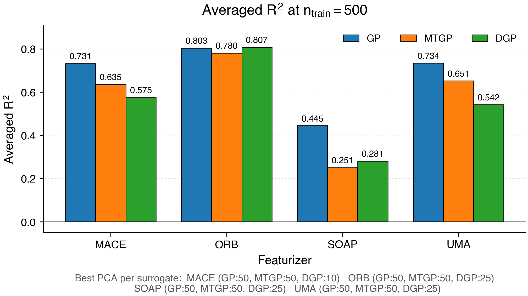
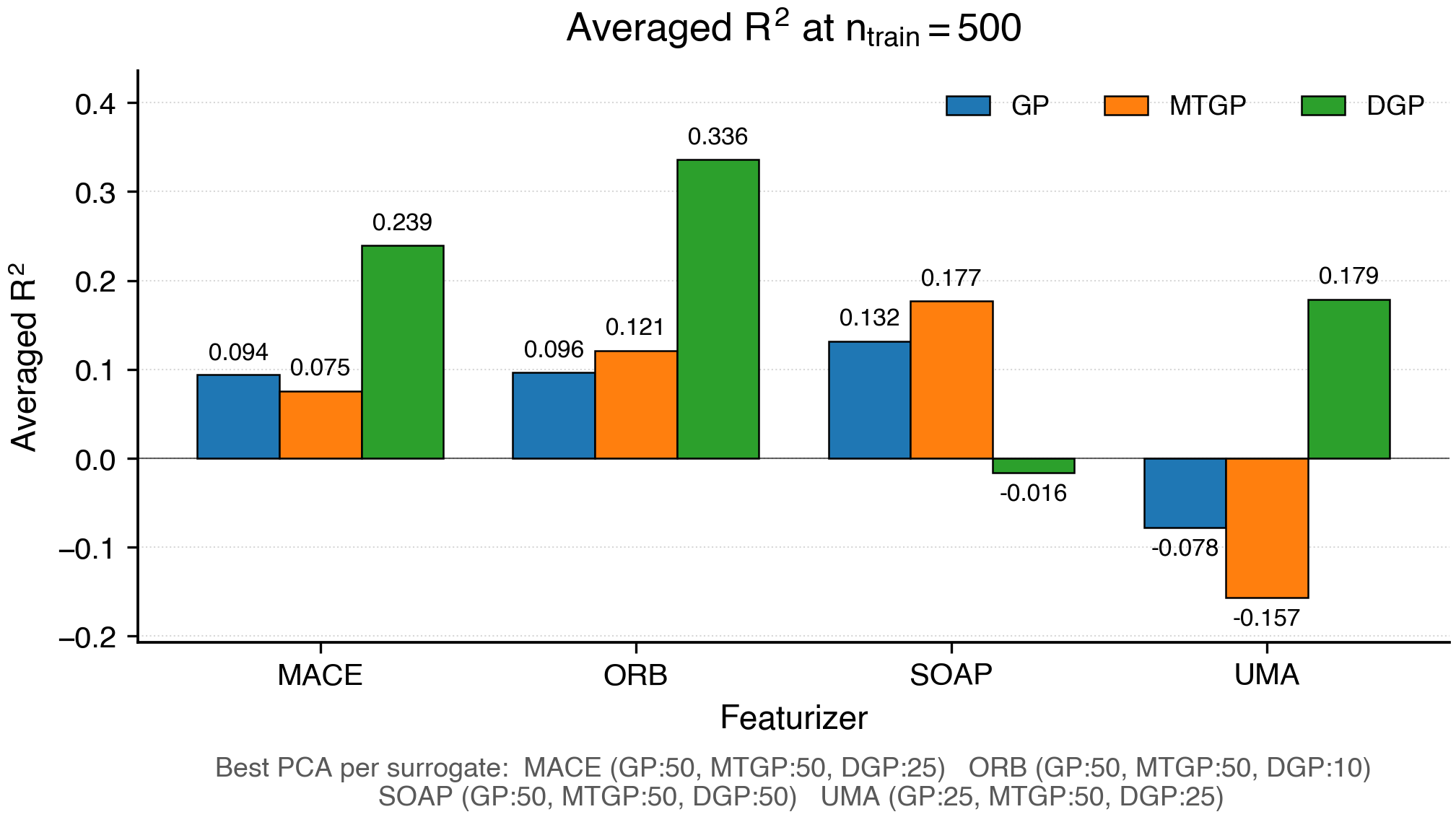
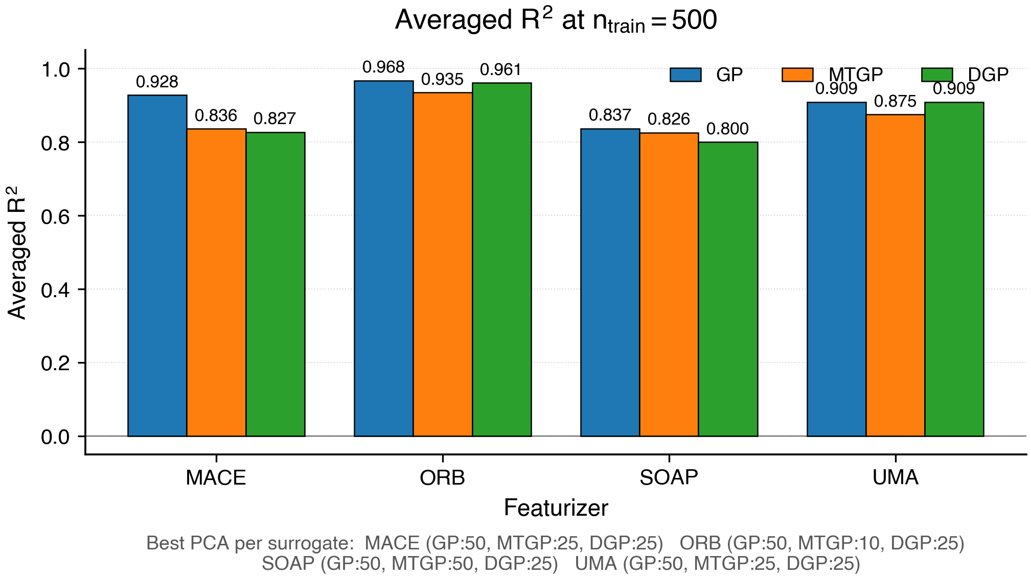
Figure 13: Averaged R\(^{2}\) across all target properties at \(n_{\text{train}}= 500\), grouped by featurizer and surrogate model, for each of the three benchmark datasets. ORB embeddings rank first in most featurizer–surrogate cells; SOAP edges ORB on the dielectric dataset under GP and MTGP. Note the different \(y\)-axis scales, which reflect the different R\(^{2}\) ranges across datasets.. a — Elastic tensor (8 properties), b — Dielectric constant (4 properties), c — Phonon thermodynamics (4 properties)
| Surrogate | Featurizer | Best PCA | Avg. | Avg.RMSE | Avg.Spearman |
|---|---|---|---|---|---|
| GP | ORB | 50 | 0.803 | 17.37 | 0.842 |
| UMA | 50 | 0.734 | 21.42 | 0.811 | |
| MACE | 50 | 0.731 | 20.46 | 0.820 | |
| SOAP | 50 | 0.445 | 33.63 | 0.688 | |
| MTGP | ORB | 50 | 0.780 | 19.30 | 0.843 |
| UMA | 50 | 0.651 | 25.80 | 0.780 | |
| MACE | 50 | 0.635 | 25.76 | 0.758 | |
| SOAP | 50 | 0.251 | 41.34 | 0.529 | |
| DGP | ORB | 25 | 0.807 | 17.84 | 0.826 |
| MACE | 10 | 0.575 | 25.53 | 0.659 | |
| UMA | 25 | 0.542 | 26.80 | 0.696 | |
| SOAP | 25 | 0.281 | 38.78 | 0.521 |
| Surr. | Feat. | PCA | RMSE | \(\rho\) | |
|---|---|---|---|---|---|
| GP | SOAP | 50 | 0.132 | 7.60 | 0.549 |
| ORB | 50 | 0.096 | 7.84 | 0.746 | |
| MACE | 50 | 0.094 | 7.94 | 0.695 | |
| UMA | 25 | \(-\)0.078 | 8.14 | 0.609 | |
| MTGP | SOAP | 50 | 0.177 | 7.27 | 0.583 |
| ORB | 50 | 0.121 | 7.85 | 0.773 | |
| MACE | 50 | 0.075 | 7.90 | 0.715 | |
| UMA | 50 | \(-\)0.157 | 8.49 | 0.656 | |
| DGP | ORB | 10 | 0.336 | 6.88 | 0.778 |
| MACE | 25 | 0.239 | 7.31 | 0.754 | |
| UMA | 25 | 0.179 | 7.35 | 0.742 | |
| SOAP | 50 | \(-\)0.016 | 7.46 | 0.019 |
| Surr. | Feat. | PCA | RMSE | \(\rho\) | |
|---|---|---|---|---|---|
| GP | ORB | 50 | 0.968 | 159.0 | 0.986 |
| MACE | 50 | 0.928 | 257.6 | 0.969 | |
| UMA | 50 | 0.909 | 348.9 | 0.952 | |
| SOAP | 50 | 0.837 | 405.0 | 0.954 | |
| MTGP | ORB | 10 | 0.935 | 238.7 | 0.967 |
| UMA | 25 | 0.875 | 375.2 | 0.938 | |
| MACE | 25 | 0.836 | 411.6 | 0.932 | |
| SOAP | 50 | 0.826 | 439.3 | 0.948 | |
| DGP | ORB | 25 | 0.961 | 197.3 | 0.982 |
| UMA | 25 | 0.909 | 337.5 | 0.949 | |
| MACE | 25 | 0.827 | 397.6 | 0.934 | |
| SOAP | 25 | 0.800 | 473.4 | 0.921 |
Per-configuration heatmaps and PCA-sensitivity curves for all three datasets are in the Supplementary Information (Supplementary Figs. S6 and S7). Two patterns from those panels matter for the loop: the GP is the most stable surrogate at PCA = 50, and the DGP, although it reaches the best R\(^{2}\) at PCA \(\leq\) 25, collapses at PCA = 50 on all three datasets, which is why we do not adopt it as a default. The collapse of DGP at high-dimensional PCA regime can be attributed to the fact that, the learnable parameter count for DGP explodes with higher feature dimension. Hence, DGP performs poorly in small training data regime.
3.4 Data efficiency and property difficulty↩︎
ORB embeddings are data-efficient. On the elastic dataset, ORB + GP at \(n_{\text{train}}= 100\) already reaches \(\bar{R}^2 \approx 0.59\), above SOAP + GP at \(n_{\text{train}}= 500\) (\(0.445\)), so the pre-trained representation is worth roughly 400 additional training samples (Figure 14, Table 7). The DGP shows the largest relative gain with added data but starts lowest and needs about 500 samples to match the GP, so in the low-data regime at the start of a campaign the GP is the safer choice.
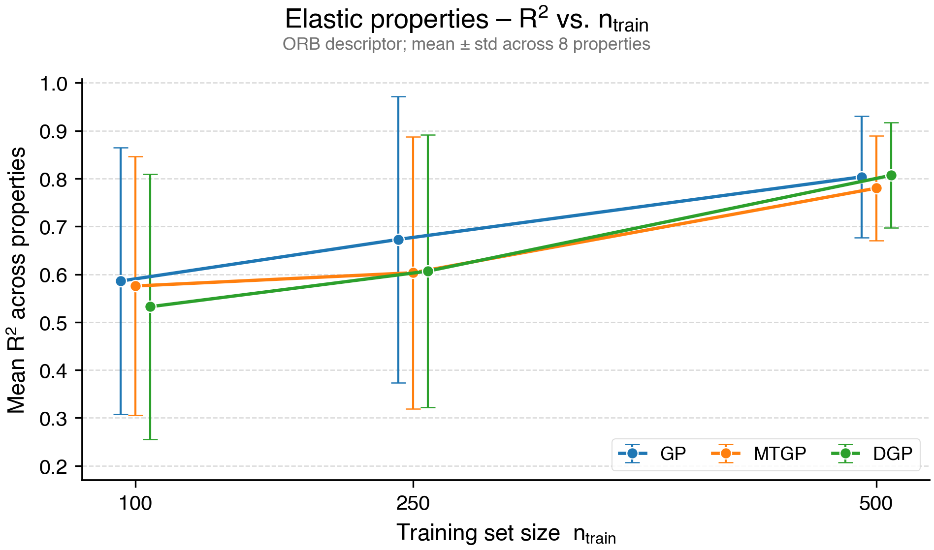
| Surrogate | \(\ntrain{=}100\) | \(\ntrain{=}250\) | \(\ntrain{=}500\) | Gain |
|---|---|---|---|---|
| GP | 0.586 | 0.673 | 0.803 | +37% |
| MTGP | 0.576 | 0.603 | 0.780 | +36% |
| DGP | 0.532 | 0.607 | 0.807 | +52% |
The three datasets form a difficulty gradient (Figure 15). Elastic moduli are the easiest: the three bulk-modulus variants reach \(R^2 > 0.91\), the shear moduli \(0.78\)–\(0.83\), with elastic anisotropy and Poisson’s ratio hardest. On the dielectric dataset only band gap is predicted well (\(R^2 = 0.852\)); the polycrystalline constants fall below zero. On the phonon-thermodynamics dataset all four targets (heat capacity \(C_v\), entropy \(S\), free energy \(F\), and the maximum phonon frequency at 300 K) are well predicted (\(R^2 = 0.93\)–\(0.98\) at the best configuration), with ORB the strongest featurizer. Per-property difficulty rankings for each dataset, the per-dataset radar profiles, and the dielectric and phonon learning curves are in the Supplementary Information (Supplementary Tables S1–S3, Supplementary Figs. S8–S10).
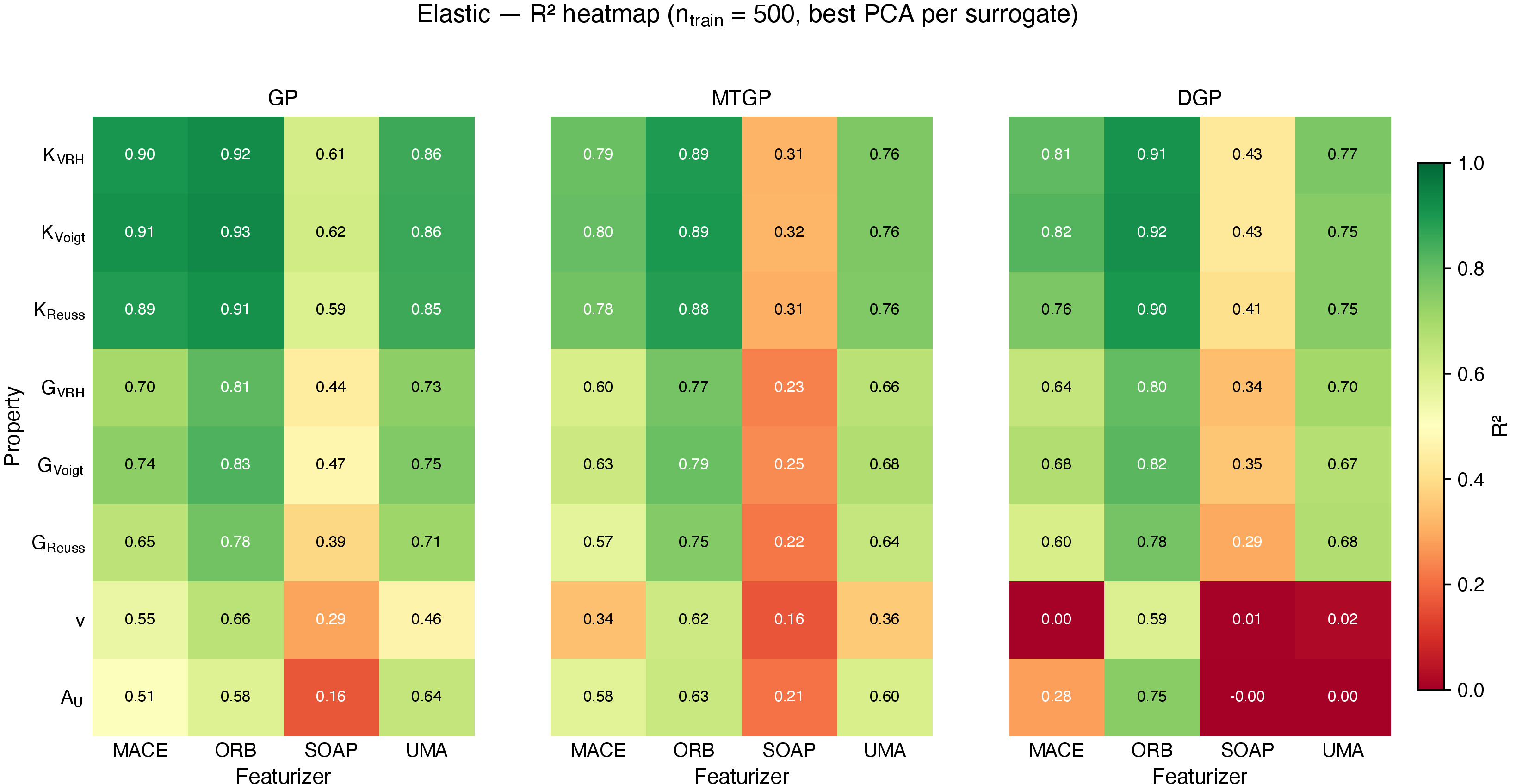
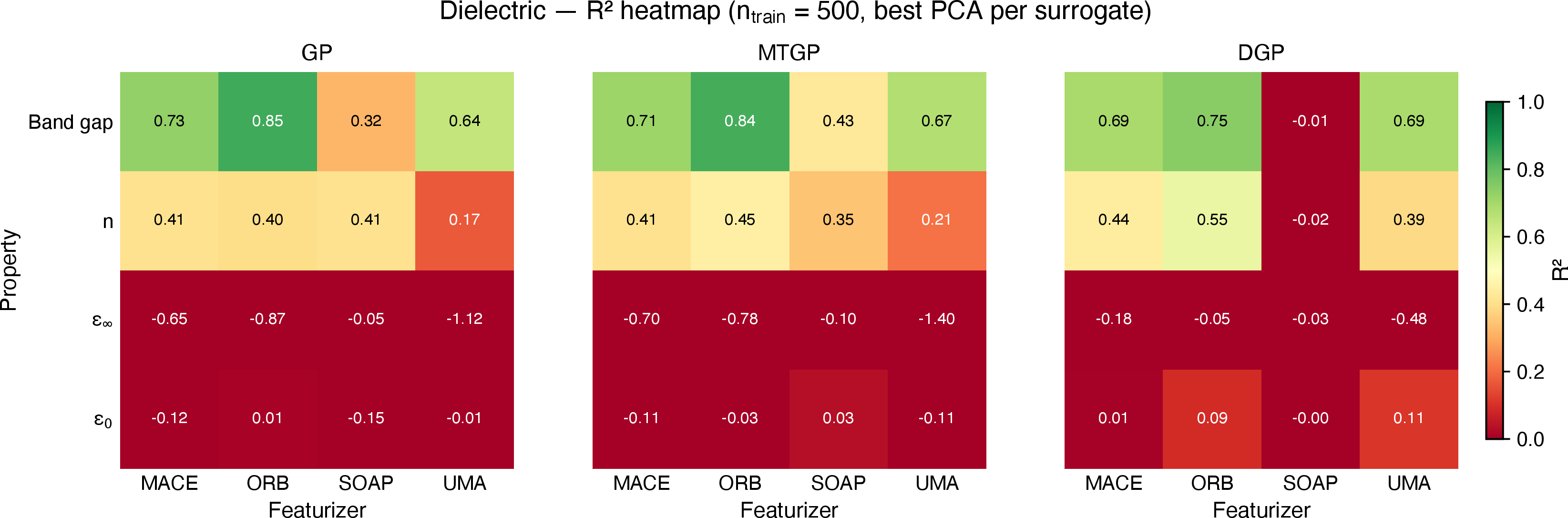
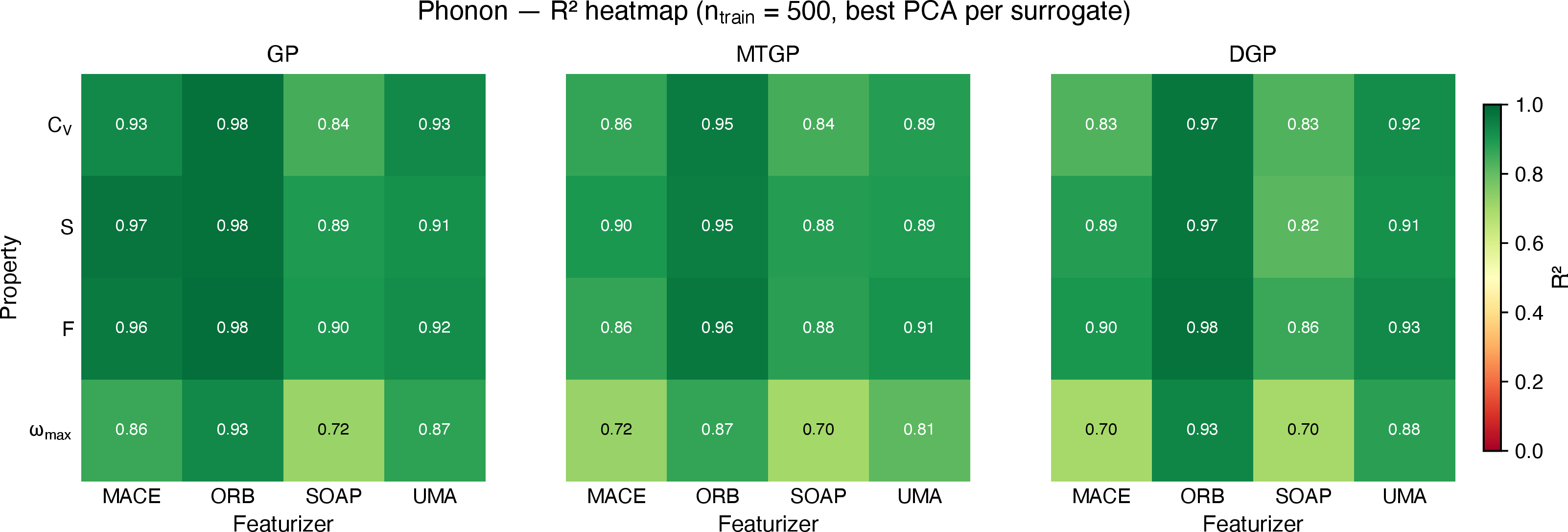
Figure 15: Property difficulty matrices showing the best-achievable R\(^{2}\) per property across all featurizer–PCA combinations at \(n_{\text{train}}= 500\), broken down by surrogate model. (a) Elastic: bulk modulus variants are easiest; anisotropy and Poisson’s ratio are hardest. (b) Dielectric: band gap is easiest; polycrystalline dielectric constants are hardest. (c) Phonon thermodynamics: heat capacity, entropy, free energy, and the maximum phonon frequency at 300 K are all well predicted.. a — Elastic tensor, b — Dielectric constant, c — Phonon thermodynamics
3.5 Cross-dataset synthesis↩︎
Table 8 collects the best configuration and the easiest and hardest property for each dataset. Three patterns recur. ORB gives the best Spearman correlation in every dataset–surrogate cell, and the best R\(^{2}\) in all but the GP and MTGP rows of the dielectric dataset, where SOAP is higher (Table 5); its R\(^{2}\) margin is largest on the elastic data (\(\Delta R^2 \approx 0.07\) over UMA and MACE) and smallest on the phonon data (\(\approx 0.04\)). The DGP collapses at PCA = 50 on all three datasets, a consequence of its two-layer variational parameters outnumbering the data at \(n_{\text{train}}= 500\), so it is accurate but fragile. The stack the closed-loop probe uses, ORB + GP + PCA = 50, follows from these patterns: ORB for accuracy and the GP for stability.
| Dataset | Best Config | Avg. | Avg.\(\rho\) | Easiest Property | Hardest Property |
|---|---|---|---|---|---|
| Elastic tensor | ORB+DGP+PCA25 | 0.807 | 0.826 | \(K_{\text{Voigt}}\) (0.931) | Poisson (0.658) |
| Dielectric | DGP+ORB+PCA10 | 0.336 | 0.778 | band_gap (0.852) | poly_elec (\(-\)0.033) |
| Phonon thermo. | GP+ORB+PCA50 | 0.968 | 0.986 | F_300K (0.984) | max_phonon_freq (0.934) |
Representative parity plots and a per-descriptor cross-dataset comparison are in the Supplementary Information (Supplementary Figs. S11–S12).
4 Discussion↩︎
4.1 Reading the closed-loop probe↩︎
The closed-loop runs in Section 3.1 insert a Gaussian-process surrogate into the published MatInvent [10] workflow without otherwise changing it. This follows two directions: adding uncertainty-aware property predictors to provide informative gradients, and moving the workflow toward closed-loop discovery. A Gaussian process is one such predictor, and the Expected-Improvement-plus-diversity gate is one minimal closed-loop step. Reviews of reinforcement-learning based fine-tuning for diffusion models [12] catalog policy-gradient and value-based families but, to our reading, do not include a Bayesian-optimization acquisition step. Recent surveys of generative models for crystals [1] cover the design space without a section on online surrogate gating, while noting the offline latent-space surrogate of Qi et al. [13] as a related precedent. Concurrent benchmarks of closed-loop discovery [39] and cross-model evaluation of crystal generators [40] are complementary. They supply environments and metrics, whereas we report one gating method run end to end across three pretrained priors.
The runs support several observations. The static-benchmark prediction carries into the loop. Both targets are well-ranked by the ORB + GP surrogate the benchmark recommends, and the gated policy (ACC) matches or exceeds ungated fine-tuning (BASE) on MatterGen and ADiT for both \(C_p\) and \(K_{\text{VRH}}\). The surrogate’s five-fold cross-validated RMSE on its accumulated training set stays flat across cycles (Figure 4), so the loop does not collapse the surrogate’s self-consistency. We do not log a per-cycle held-out regression error on each cycle’s fresh proposals; for the bulk-modulus target, however, a causal replay of the surrogate (Section 3.1.10) measures its generalization directly as a ranking on unseen proposals (\(\rho = 0.944\)), and the gain is in any case consistent with the static-benchmark prediction and is not accompanied by surrogate breakdown on the training points.
Seed distributions are more informative than best-of-run values. Best-value summaries in Figure 8 make MatterGen and CrystalFlow look interchangeable on \(C_p\), and place ADiT far ahead on \(K_{\text{VRH}}\) on the strength of a single 375 GPa polymorph. The mean of the top three candidates narrows these gaps to within overlapping error bars on both targets (\(C_p\): \(1.11 \pm 0.56\), \(0.89 \pm 0.40\), \(0.80 \pm 0.18\) J/g/K; \(K_{\text{VRH}}\): \(273 \pm 37\), \(224 \pm 43\), \(259 \pm 45\) GPa). At a limited compute budget, reporting maxima per backbone overstates the difference between priors, and seed distributions are the safer comparator.
The priors differ more in the geometry of their top structures than in the property values those structures reach. The crystal-system histograms in Figure 6 show CrystalFlow and ADiT drawing most top hits from triclinic and monoclinic systems, while MatterGen produces the only tetragonal hits and a flatter distribution. This tracks each prior’s training: MatterGen learns Materials Project ground states, which are symmetry-rich, whereas the learned manifolds of CrystalFlow and ADiT contain many more low-symmetry than high-symmetry states. When the target property favors high symmetry, a symmetric prior helps; when it does not, the bias is neutral.
Across backbones, the gain from the gate is consistent but modest, with its size set by the prior. The discovery curves separate ACC from BASE by 0.05–0.23 J/g/K on \(C_p\) and 10–50 GPa on \(K_{\text{VRH}}\), largest where the prior already concentrates in the target region (MatterGen, ADiT) and smallest where seed-to-seed variance is high (CrystalFlow). The gate cannot rescue runs whose diffusion samples never enter the relevant region.
The gate also saves oracle calls, by a margin that depends on the backbone. The gate caps oracle calls at \(K = 4\) per cycle, so it saves calls whenever the rate of structures surviving the stability filter exceeds four per cycle. Every (backbone, target) cell clears that rate, with roughly 6–16 SUN-survivors dispatched per cycle, so the gated policy reduces oracle calls in all of them, by \(1.8\)–\(3.5\times\) (Section 3.1.4; Supplementary Fig. S2). The gate therefore lowers oracle cost in every cell we ran, while in general bounding it to the fixed per-cycle budget.
Pretrained priors alone do not break through their own ceilings. The \(\sim\)1.2 J/g/K plateau in \(C_p\) and the \(\sim\)310 GPa plateau in mean \(K_{\text{VRH}}\) reflect what each backbone can reach under policy-gradient rollouts without property-conditional updates. Moving past these ceilings will require fine-tuning the priors toward the target property, or a more exploratory acquisition rule than Expected Improvement with diversity. The probe supports the surrogate-gated diffusion loop as a working unit; it does not single out any one backbone or oracle as the recommended choice for a discovery campaign.
4.2 Contribution of the static benchmark↩︎
The benchmark explains why the loop’s stack (ORB + GP + PCA = 50) is a reasonable default rather than the only choice. Among the four embeddings, pre-trained ORB was the most reliable across the three datasets and most surrogates, which we attribute to the scale and diversity of its pre-training (OMat24, over \(10^{8}\) configurations) and to a compact embedding whose leading principal components already carry property-relevant variation: ORB at 10 components matches or exceeds SOAP at 50 on the elastic and phonon datasets. The exception is the electronic dielectric dataset under GP and MTGP, where SOAP’s explicit local-environment encoding gives a higher R\(^{2}\) than ORB; ORB recovers under the DGP. UMA/eSEN and MACE track each other closely, suggesting they sit at a similar representational level that only larger pre-training corpora would surpass.
Surrogate choice follows a simple rule. The GP at PCA = 50 is a safe default that trains in seconds and needs no tuning beyond marginal-likelihood optimization. The DGP gives the best R\(^{2}\) on the elastic and dielectric datasets when its input is kept to PCA \(\leq\) 25, but at PCA = 50 with \(n_{\text{train}}= 500\) its variational parameters outnumber the data and the fit degrades, so PCA dimension should be treated as a tuned hyperparameter when using it (Supplementary Fig. S13). The multi-task GP helps only when a few (\(T \leq 4\)) physically related properties are predicted together, especially with a weaker featurizer; with eight largely independent elastic targets it shows negative transfer [51], and the independent GP is preferable. The dielectric learning curves (Supplementary Fig. S9) show Spearman correlations holding with training size even where R\(^{2}\) falls.
The datasets span a gradient of difficulty set by the distance between crystal geometry and the target property. Elastic and phonon-thermodynamic targets, governed by bond stiffness, atomic mass, and lattice vibrations, are predicted well; the electronic dielectric responses, which depend on many-body polarization and electronic structure, are not (\(\bar{R}^2 \lesssim 0.34\)). For geometry-dominated targets the pipeline applies directly; for the electronic dielectric targets it can still guide a ranked search (\(\bar{\rho}\) up to \(\approx 0.78\) even where \(\bar{R}^2 \lesssim 0.34\)), though absolute prediction would need electronic-structure-aware embeddings. A practical consequence for Bayesian optimization is data efficiency: ORB embeddings reach SOAP + GP’s \(n_{\text{train}}= 500\) accuracy at \(n_{\text{train}}= 100\), which shortens the warm-up phase of a campaign where each evaluation is an expensive calculation. Surrogate accuracy is necessary but not sufficient, however, since acquisition also depends on uncertainty calibration, which we do not assess here.
5 Conclusion↩︎
A surrogate gate turns a generative diffusion loop from an oracle-bound search into a budgeted one. Placing a Gaussian process with an Expected Improvement along with diversity rule between the structure filter and the property oracle of RL-steered generative workflow, we found that the gate matches or exceeds ungated fine-tuning on MatterGen and ADiT for both heat capacity and bulk modulus while holding oracle calls to a fixed per-cycle budget. Budget-matched ablations attribute the gain to the surrogate’s ranking-based selection rather than the reduced number of oracle calls: at four oracle calls per cycle the gate outperforms arbitrary selection, and it comes within roughly nine percent of exhaustive oracle search at about a fifth of the cost in the most competitive instance. None of the top structures it retrieves match the warm-start pool, so the gate steers the generator rather than replaying it. In our benchmark of 8,640 surrogate fits, among the embeddings we tested, pre-trained ORB with a Gaussian process was the most reliable choice across mechanical, electronic, and vibrational properties, and we adopt it as the default in the loop.
There are some limitations that can be addressed in future works. The oracle is a learned surrogate, DFT-validated here for the bulk-modulus target but not for heat capacity, the in-loop ablations probe one backbone in depth, and we report seed distributions rather than best-of-run maxima. We close part of this gap here, validating the bulk-modulus discoveries against DFT and measuring the surrogate’s generalization as a causal held-out ranking; the heat-capacity DFT validation, property-conditional fine-tuning of the priors, and a per-cycle held-out regression signal for the gate remain the natural next steps. The complete pipeline, aggregated results, and analysis scripts are released as open-source software.
Code and Data Availability↩︎
The elastic and dielectric datasets are publicly available through the matminer library [24]; the phonon dataset is drawn from the Materials Project DFPT phonon database [25]. The complete static-benchmark pipeline (featurization, surrogate training, and evaluation scripts), together with the aggregated holdout CSVs that drive every figure in the paper, is available at https://github.com/sheikhahnaf/matgen-BO/tree/main. The same repository contains the closed-loop probe of Section 3.1, including our modified MatInvent codebase with diffusion adapters for MatterGen, CrystalFlow, and ADiT, the GP-routed acquisition gate (Expected-Improvement plus Determinantal-Point-Process diversity), the heat-capacity and bulk-modulus oracles, all SLURM batches, and the curated per-trajectory results used to make the closed-loop figures, together with the ORB-PU synthesizability classifier of Section 2.8; its eight Optuna-tuned checkpoints along with the checkpoints of the generative models from the RL cycles are archived at https://huggingface.co/SheikhAhnaf/apu-synthesizability-checkpoints.
Conflicts of Interest↩︎
There are no conflicts of interest to declare.
Author Contributions↩︎
Sk Md Ahnaf Akif Alvi: Conceptualization, Methodology, Software, Validation, Investigation, Data curation, Visualization, Writing – original draft. Jan Janssen: Methodology, Resources, Writing – review & editing. Danny Perez: Conceptualization, Methodology, Supervision, Writing – review & editing. Douglas Allaire: Methodology, Supervision, Writing – review & editing. Raymundo Arróyave: Conceptualization, Funding acquisition, Project administration, Supervision, Writing – review & editing.
Acknowledgments↩︎
This material is based on work supported by the Texas A&M University System National Laboratories Office of the Texas A&M University System and Los Alamos National Laboratory as part of the Joint Research Collaboration Program. The authors acknowledge the support from the U.S. Department of Energy (DOE) ARPA-E CHADWICK Program through Project DE-AR0001988. RA acknowledges the support from the WoodNext Foundation for their support of the Aggie AI Foundry. The authors acknowledge computational resources provided by the Texas A&M High Performance Research Computing (HPRC) facility. Sk Md Ahnaf Akif Alvi acknowledges an NSF ACCESS Explore allocation (project MAT250131, “Advanced Surrogates-based Bayesian Optimization for Materials Discovery in High Entropy Alloy Spaces”); this work used the ACES accelerator testbed at Texas A&M University through allocation MAT250131 from the Advanced Cyberinfrastructure Coordination Ecosystem: Services & Support (ACCESS) program, which is supported by U.S.National Science Foundation grants #2138259, #2138286, #2138307, #2137603, and #2138296.