WARP-RM: A Warp-Augmented Relative Progress Reward Model for Data Curation
June 26, 2026
Abstract
Scaling imitation learning requires large datasets, yet human teleoperation inevitably produces mixed-quality demonstrations containing hesitations and recoveries. Prior frame-level progress reward models supervise on absolute temporal progress proxies that suffer from label noise, or require costly human annotations to define subtask boundaries. We present WARP (Warp-Augmented Relative Progress), a novel fully self-supervised algorithm for learning dense, signed relative progress magnitudes directly from successful demonstrations. WARP generates per-frame progress targets via time-warp augmentations of demonstrations (variable playback speeds and reversals) and we train WARP-RM to predict the normalized elapsed time between input frames. Aggregating these predictions across overlapping windows yields a dense frame-level progress signal. We then introduce WARP-BC, which leverages these scalar reward estimates to upweight high-advantage action chunks during behavior cloning, where chunk-level advantage is obtained by aggregating per-frame rewards. We evaluate our approach on a physical bimanual robot system performing a long-horizon deformable object manipulation task: folding T-shirts from a random crumpled start. To evaluate policy robustness against suboptimal data, we construct training datasets of varying quality using episode length as a proxy for teleoperation sub-optimality. As the dataset is widened to admit more inefficiencies, WARP-BC maintains a 19/20 success rate compared to vanilla BC’s collapse to 2/20, improving throughput by up to \(\sim\!\boldsymbol{18}\times\).
Project page: https://uynitsuj.github.io/warp-rm/.
1 Introduction↩︎
Imitation learning has emerged as a powerful framework for long-horizon robot manipulation, enabling complex visuomotor behaviors from human teleoperated demonstrations. Recent advances in policy modeling and large-scale pretraining [1]–[9] have significantly improved expressivity and generalization. However, these methods remain highly sensitive to demonstration quality, particularly in long-horizon manipulation settings, as policies learn to mimic suboptimal pauses and fumbles present in human teleoperation [10]–[12]. If trained on, these behaviors can derail policy performance. However, suboptimal sequences often contain valuable recovery behaviors, akin to DAgger data [13]–[17]. Some approaches to data curation operate at the trajectory level, discarding entire episodes that fall below a quality threshold [18]–[20]. However, this coarse filtering may suffer from two limitations: it discards valuable, high-advantage segments embedded within otherwise suboptimal executions, while simultaneously failing to prune localized hesitations or fumbles within retained demonstrations.
To address the limitations of episode-level filtering, recent methods instead learn frame-level progress signals for localized data curation. Most existing progress reward models operate in an absolute progress regime. Methods like ReWiND [21] use normalized episode duration as a supervision target, while representation learning techniques like VIP [22] and LIV [23] rely on temporal contrastive alignment to globally map visual observations. However, equating elapsed timesteps or global temporal alignment with task progress introduces considerable label noise. Because temporal progression does not guarantee task progression, two demonstrations at the same normalized frame index may reflect entirely different stages of the task due to pauses, failed grasps, or varying operator strategies [24]. More recent frame-level dense reward models address this noise with human annotations [25], [26], but this is costly to scale and often inconsistent.
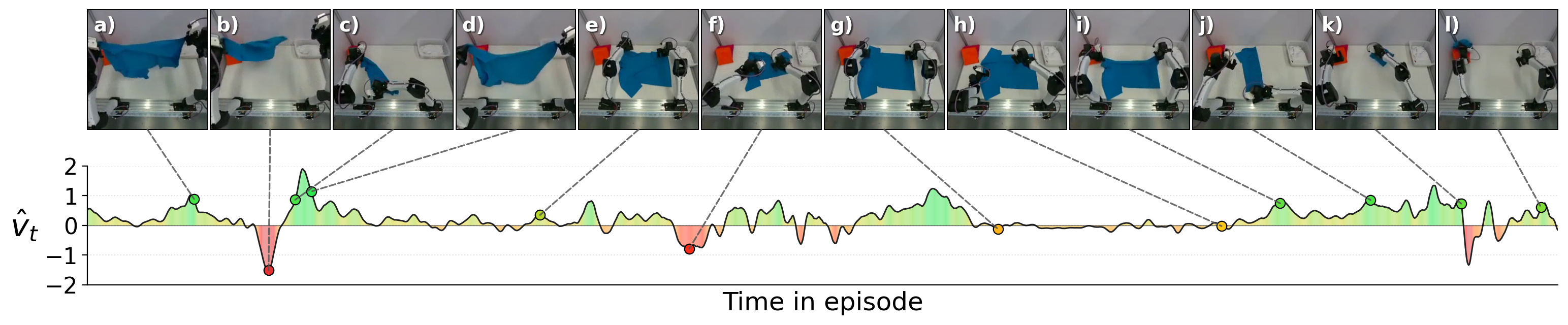
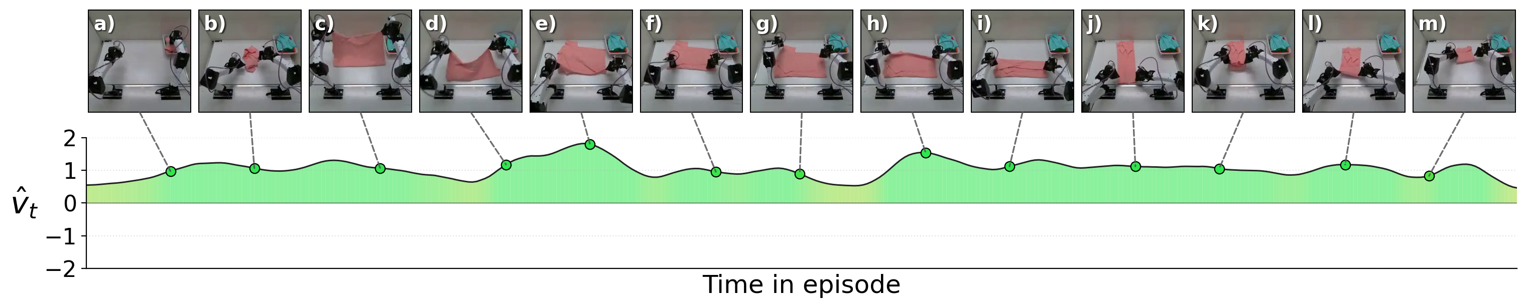
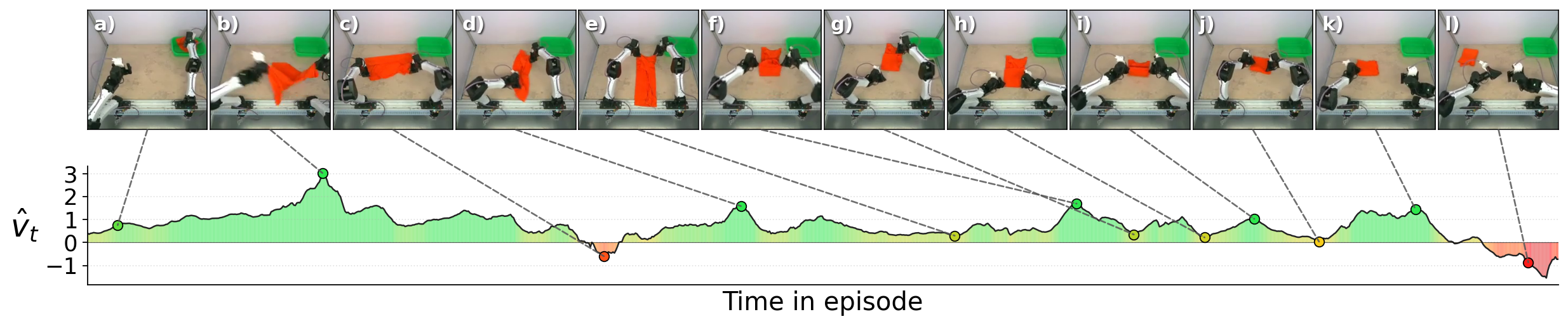
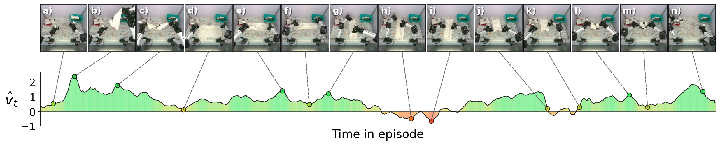
We propose WARP, a fully self-supervised method that learns a local relative progress signal. We construct per-frame cumulative progress labels by replaying successful demonstrations at non-uniform velocities including in reverse. A model trained to predict these velocities from a sequence of images yields a frame-level progress-velocity signal of how fast and in which direction the task is advancing: large positive values during decisive forward progress, near zero during pauses or fumbles, and negative during state regression. Aggregating these predictions yields a dense progress signal that identifies decisive progress, stagnation, and regression. We then introduce WARP-BC, which uses these scores to filter and reweight action chunks during behavior cloning.
This paper makes three contributions:
WARP, a fully self-supervised algorithm that learns a dense relative task progress signal via a novel time-warping augmentation. We apply this method to train WARP-RM, a relative progress model that generates a signal indicating local task progress, given a demonstration.
WARP-BC, which uses WARP-RM’s frame-level estimates to gate and reweight action chunks in the behavior cloning objective. We show (Sec. 4) that gating and reweighting by the terminal-frame progress velocity outperforms chunk-mean aggregation.
We evaluate WARP-BC across 420 real-world trials on a physical bimanual robot spanning two manipulation tasks. On T-shirt folding from a crumpled start, as the policy training dataset admits more inefficient demonstrations, vanilla BC collapses to a 2/20 success rate, while WARP-BC remains robust at 19/20 and yields up to an \(\sim\!18\times\) improvement in successful folding throughput.
2 Related Work↩︎
Time Warping for Video Representation Learning. Predicting temporal transformations has been explored as a self-supervised objective for video representation learning. Many methods apply a uniform speed transformation and use speed classification as a self-supervised objective [27]–[30]. A smaller body of work employs discrete, per-frame-independent warping, sampling the number of frames to skip at each timestep from a discrete set and training a classifier to predict the skip count per frame [31], [32]. In contrast, WARP models time warping as a structured stochastic process that produces smoothly correlated, non-uniform speed variations spanning slow-motion to fast-forward playback. Rather than serving as a pretext task for representation learning, WARP uses time warping as an augmentation directly for its end task: progress estimation.
Data Curation for Robot Imitation Learning. Offline policy learning performance degrades substantially when training on mixed-quality human data containing variations in operator proficiency, trajectory length, and solution strategy [10]. Prior work has explored demonstration data curation at varying levels of granularity to address sensitivity to suboptimal demonstrations. At the dataset level, Re-Mix [33] optimizes over data sources to create large multi-dataset mixtures. At the episode level, DemInf [19] uses a mutual information approach to curate episodes, while other works use influence function based approaches [18], [20].
Progress Reward Models. Rather than operating at the episode level, reward and progress models learn a dense frame-level quality signal within a demonstration, enabling finer-grained data curation. Most prior progress models operate in an absolute progress regime: each frame is assigned a target value on a globally normalized \([0,1]\) completion axis, either from its position within the demonstration or from human-annotated subtask boundaries. ReWiND [21] supervises on normalized frame indices, while VIP [22] and LIV [23] use temporal contrastive learning to align representations with absolute task progression. We argue that this becomes a limitation for long-horizon teleoperation. Operators may pause, retry, or recover at different points, thus the same normalized timestamp can correspond to substantially different task states across demonstrations, injecting noise into any model that supervises against the absolute axis. In contrast, WARP models relative progress velocity: whether a short temporal segment moves the task forward or backward, and by how much. This formulation avoids requiring cross-demonstration temporal alignment while still producing a dense scalar signal suitable for action-chunk reweighting.
Closest to our work, SARM [25] and ARM [26] leverage human annotated data to train progress reward models and use the learned models to reweigh action chunks, performing Reward-Aligned Behavior Cloning (RA-BC). SCIZOR [34] trains a self-supervised progress estimator which predicts the time between two frames to curate large multi-task datasets for behavior cloning. WARP-BC additionally weights retained chunks in proportion to their magnitude. Other works [35]–[38] explore multi-task reward modeling using large vision-language models (VLMs). While these methods demonstrate impressive semantic generalization, they often trade high-frequency temporal resolution for this breadth. For instance, methods relying on token-probability extraction [36] or trajectory-level preference comparisons [35] require VLM queries that necessitate coarser frame subsampling, limiting sensitivity to higher frequency temporal variations critical for dynamic control. Furthermore, because these models frequently anchor on absolute progress [35] or discretized semantic milestones [37], they remain susceptible to cross-demonstration temporal alignment noise.
3 Method↩︎
3.1 Overview and Notation↩︎
We introduce the Warp-Augmented Relative Progress Reward Model (WARP-RM), a vision-based model that estimates the dense, per-frame progress velocity of a task directly from visual observations. To train WARP-RM without human annotations, we propose the WARP algorithm, a fully self-supervised method that trains the model to predict the normalized time delta for each frame relative to a starting frame, using a dataset of successful human teleoperated demonstrations. We hypothesize that time-warping video playback speed—and its corresponding progress label—provides a strong self-supervised signal: subsampling frames at wider intervals simulates faster execution, while sampling at narrower intervals simulates slower execution. By varying this time-warping augmentation non-uniformly, a single demonstration provides dense supervision over a continuous range of progress velocities.
A demonstration consists of a sequence of \(T\) RGB frames \(o_0, \dots, o_{T-1}\) recorded at a fixed frequency, from which a frozen visual encoder \(\phi\) produces a per-frame feature vector. From each demonstration we sample a window of \(N\) frame indices \(i_0, \dots, i_{N-1}\) via a time-warping procedure that replays the demonstration at varying speeds and directions, so the indices may be non-monotonic and non-linear. Each index has a corresponding pseudo-label \(y_k\): the normalized time delta from \(o_{i_0}\) to \(o_{i_k}\), representing the cumulative temporal displacement from the start of the window.
WARP-RM is trained to predict \(y_1,...y_{N-1}\) given the set of visual features \(\phi(o_{i_0}), ..., \phi(o_{i_{N-1}})\). At inference the model is given a sequence of frames spaced linearly with a canonical inter-frame stride of \(S\) seconds covering a window of \(L = (N-1)S\) seconds, and predictions are aggregated following the procedure in Sec. 3.5. This assigns each frame a scalar signed progress velocity \(v_t\) measuring how fast and in which direction the task is progressing, calibrated so that: \(\hat{v}_t \approx 1\) matches the pace of the average reference demonstrations, \(\hat{v}_t \approx 0\) is stalling progress, and \(\hat{v}_t < 0\) is regressing progress.
3.2 Time-Warp Sampler↩︎
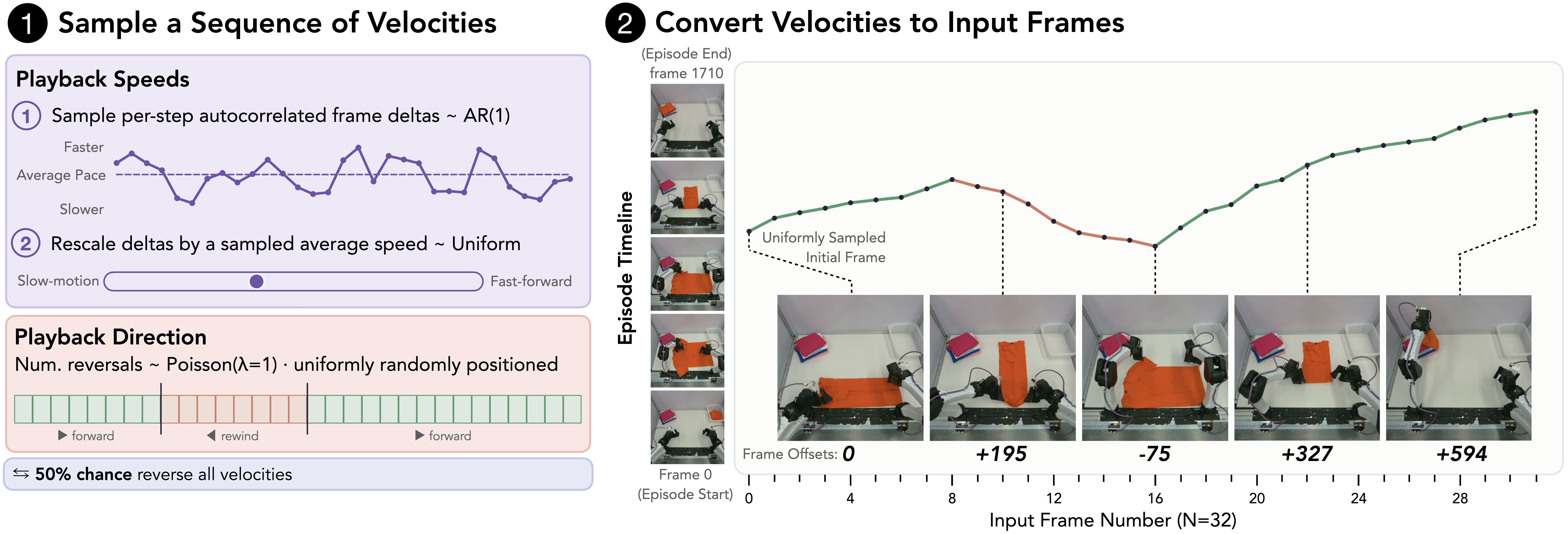
The sampler produces a set of indices \(i_0,...i_{N-1}\) through the following procedure. First, \(N-1\) relative log-velocities are drawn from a stationary AR(1) process with autocorrelation \(\alpha\) and marginal standard deviation \(\sigma_\infty\): \[z_0 \sim \mathcal{N}(0,\,\sigma_\infty^2), \qquad z_k = \alpha\, z_{k-1} + \sqrt{1-\alpha^2}\,\sigma_\infty\,\epsilon_k,\quad \epsilon_k \sim \mathcal{N}(0,\,1),\quad k = 0, \dots, N-2 \label{eq:ar1}\tag{1}\]
Operating in log-space ensures that a 2x speedup and a 0.5x slowdown are equally likely, while keeping all velocities strictly positive; reversals are sampled separately. Initializing \(z_0\) from the marginal distribution makes the process stationary, so the log-velocity variance is constant across all \(N-1\) steps. The autocorrelation parameter \(\alpha\) controls the smoothness of velocity changes between consecutive frames. These log-velocities are exponentiated to get \(\tilde{v}_t = e^{z_t}\), an unnormalized set of velocities.
Next, the total path length \(\ell\) that the indices will span is sampled from Uniform\(([\frac{1}{3}L, \frac{5}{3}L])\), ensuring the model sees both slow-motion and fast-forwarded views during training. The sampled velocities are rescaled so they sum to \(\ell\):
\[\tilde{u}_{k} = \ell \cdot \tilde{v}_{k} \big / {\textstyle \sum_{j=0}^{N-2}\tilde{v}_{j}} \quad k=0,...,N-2 \label{eq:rescale}\tag{2}\]
The resulting \(\tilde{u}_k\) are all non-negative, meaning they correspond to forward progress. However, as suggested by ReWiND, reversing playback can mimic failed policy rollouts providing supervision of negative progress [21]. The time-warp sampler extends this idea by adding a variable number of reversals in each playback.
To simulate non-monotonic progress, the sampler draws \(R \sim \mathrm{Poisson}(\lambda_{\text{rev}})\) reversal points and selects their locations uniformly randomly without replacement from \(\{1,..., N-1\}\). At each reversal point, the sign of all subsequent velocities is flipped causing the trajectory to alternate between forward and backward playback. Finally, the entire trajectory is reversed with probability \(0.5\), ensuring the reward model sees a roughly equal amount of increasing and decreasing progress samples. This results in a set of signed, normalized playback velocities \(u_0, ..., u_{N-1}\).
Let \(c_j = \sum_{k=0}^{j-1} u_k\) denote the cumulative signed displacement at step \(j\), with \(c_0 = 0\). The first index \(i_0\) is drawn uniformly from the integer range \([\lceil -\min_j c_j \rceil,\; \lfloor T - 1 - \max_j c_j \rfloor]\), the set of starting positions for which all subsequent indices fall within \([0, T-1]\). The remaining indices follow as \(i_j = \mathrm{round}(i_0 + c_j)\).
3.3 Progress Model Training↩︎
Relative Cumulative Progress Targets. From the sampled indices, the per-frame cumulative progress pseudo-labels are computed as the signed displacement from the window start normalized by a constant \(C_{\text{norm}}\): \[y_j \;=\; (i_j - i_0) / C_{\text{norm}}, \qquad j = 0, \dots, N{-}1 \label{eq:rel95label}\tag{3}\]
Categorical Objective. Given the visual features \(\phi(o_{i_0}), ..., \phi(o_{i_{N-1})}\) the progress model is trained to predict \(y_0, ..., y_{N-1}\). Rather than regressing directly on \(y_j\), WARP-RM predicts \(N\) separate probability distributions over evenly spaced categorical bins. The model is trained with a cross-entropy loss against a two-hot target encoding that encodes a continuous value by finding the coefficients for linear interpolation from the two nearest bin centers. This categorical classification approach mitigates optimization instabilities and capacity underutilization typically found in direct regression [39].
3.4 Model Architecture↩︎

Similar to SARM [25], the model architecture uses a frozen visual backbone and transformer temporal aggregator, but it replaces the stage classifier and subtask-progress regressor with a single progress velocity head (Figure 3). WARP-RM uses a frozen DINOv3 ViT-B/16 [40] as \(\phi\), yielding a \(768\)-dimensional feature vector per frame. Each input token is formed by concatenating the frame embedding with its temporal difference: \([\phi(o_{i_j}),\, \phi(o_{i_j}) - \phi(o_{i_{j-1}})] \in \mathbb{R}^{1536}\), with the difference set to zero for \(j=0\). Tokens are projected to the transformer dimension, augmented with fixed sinusoidal positional embeddings, and processed by a bidirectional Transformer encoder. Finally, a linear layer maps each output token to separate probability distributions. At inference, the predicted \(\hat{y}_j\) is computed as the expectation of the predicted distribution.
3.5 Warp-Augmented Relative Progress Behavior Cloning↩︎
WARP-BC aggregates predictions from WARP-RM into dense, per-frame progress velocities and uses them for action-chunk-level reweighting of the imitation-learning loss.
Velocity Aggregation. We apply WARP-RM in overlapping windows, each containing \(N\) frames separated by the canonical stride of \(S\) seconds, with consecutive windows shifted by a single source-frame. Within each window, consecutive expected cumulative progress predictions are differenced and scaled to produce a sequence of intra-window velocities: \(v_j = (N-1)(\hat{y}_j - \hat{y}_{j-1})\). Each interior source-frame \(t\) in the episode is covered by multiple overlapping windows. The final per-frame progress velocity, \(\hat{v}_t\), is computed as the mean of all intra-window velocity predictions \(v_j\).
Action Chunk Weighting. The behavior cloning policy is trained to predict one second action chunks. The velocity at the final frame of the action chunk, \(\hat{v}_{\text{end}}\), is used to compute the reward-aligned behavior cloning (RA-BC) weight \(w(s, a)\) for each state-action pair: \[w(s, a) \;=\; \hat{v}_{\text{end}} \, \cdot \, \mathbb{1}_{\, \hat{v}_{\text{end}} \,>\, \tau \,} \label{eq:warpbc95weight}\tag{4}\] Chunks with \(w(s, a) = 0\) are filtered out prior to training to avoid reducing effective batch size, following advantage-filtered behavior cloning [41]. Here \(\hat{v}_{\text{end}}\) acts as an empirical progress velocity-based proxy for advantage rather than an explicitly estimated RL advantage with a value baseline.
Behavior Cloning Objective. The final policy loss is the standard flow-matching loss weighted per-sample by \(w(s, a)\): \[\mathcal{L}_\text{BC} \;=\; \mathbb{E}_{(s, a) \sim \mathcal{D}}\, [w{(s,a)} \cdot \mathcal{L}_\text{flow}(\pi_\theta; s, a)]. \label{eq:bc95loss}\tag{5}\]


4 Experiments↩︎
Each policy is evaluated on a bimanual I2RT YAM robot arm setup over \(20\) trials1 of T-shirt folding using a variety of differently colored medium-sized T-shirts not seen during training. In each trial, the robot must retrieve a crumpled shirt from a bin containing a variable number of shirts, flatten it on the workspace, fold both sleeves inward, fold the shirt in half twice, and move it towards the top-left corner of the workspace to complete the task. If the policy does not complete the task within 240 seconds, the trial is marked as a failure. This time budget is chosen as 2\(\times\) the longest training demonstration, providing a generous margin for retry behaviors while bounding evaluation time. Time-to-completion (TTC) is reported as the average completion time for successful trials. Throughput is the number of successful folds per hour, with each failed trial contributing its four-minute timeout to the denominator; human reset time between trials is excluded from this calculation.
4.1 Implementation Details↩︎
We use \(N=32\) frames, stride \(S=1.5s\), AR(1) parameters \(\alpha=0.5, \sigma_{\infty}=\ln 2\), reversal rate \(\lambda_{rev}=1\), and filtering threshold \(\tau=1.0\) (reweighting only chunks above the reference expert pace, \(\hat{v}_{\text{end}} > 1\)). See Appendix 8 for additional details.
4.2 Policy Training Datasets and Tiers↩︎
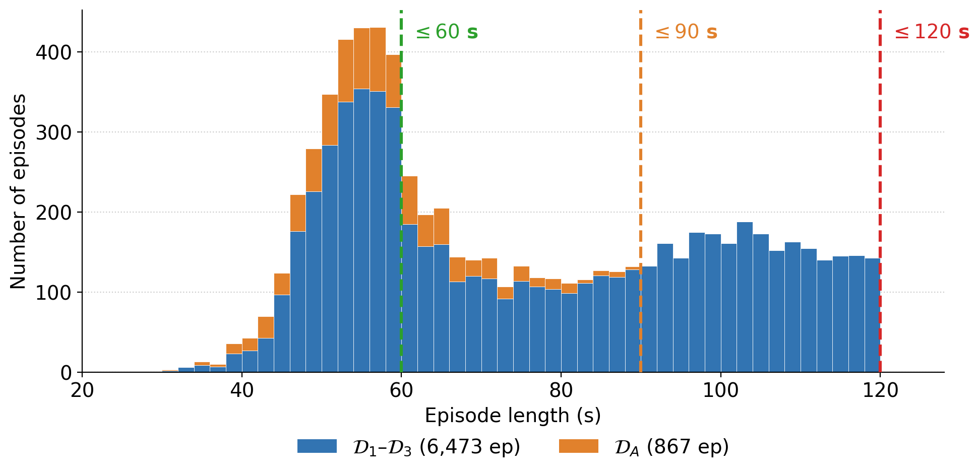
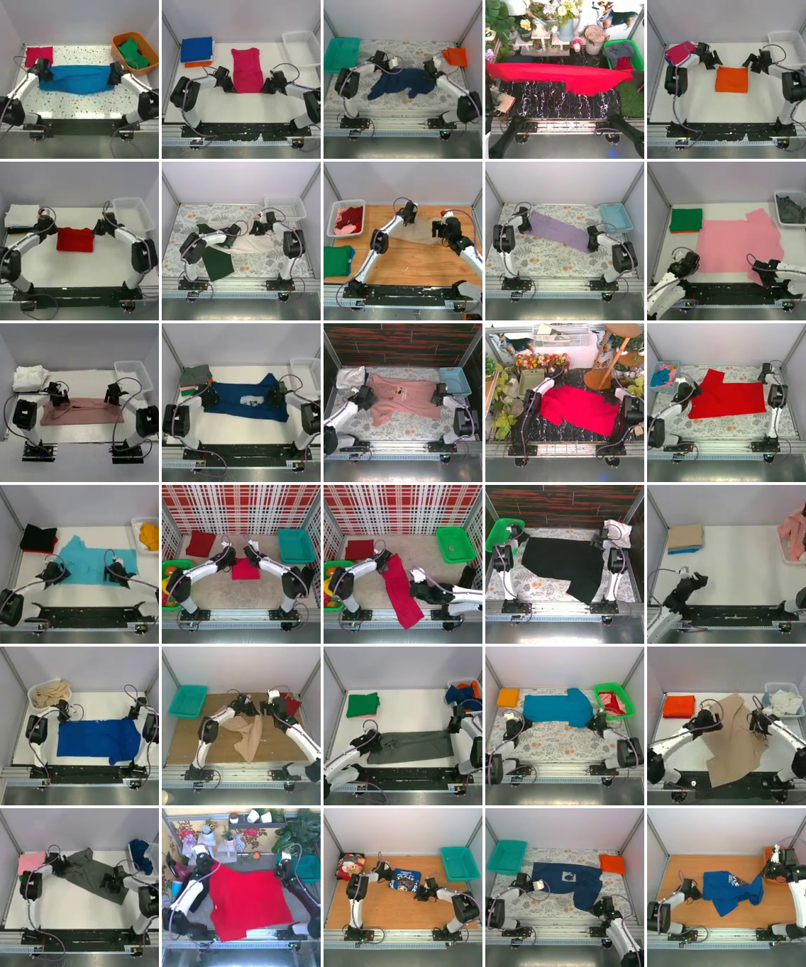
All policy training datasets are length-filtered subsets of a single larger dataset of successful human-teleoperated T-shirt-folding demonstrations. On this task, episode length serves as a coarse proxy for execution efficiency: longer episodes tend to contain more hesitations, retries, and recoveries. The episode-length distribution exhibits a dominant mode near 50–60 seconds with a broader tail beyond 85 seconds (see Appendix 6 for histogram). To systematically evaluate robustness as more inefficient behavior is admitted into training, we define three tiers: \(\mathcal{D}_1\) (\(\le 60\)s): 2,427 episodes (36.1 hours), \(\mathcal{D}_2\) (\(\le 90\)s): 4,124 episodes (71.3 hours), and \(\mathcal{D}_3\) (\(\le 120\)s): 6,473 episodes (139.7 hours). Policies are trained either with uniform weighting (vanilla BC) or WARP-based progress reweighting on the same underlying demonstrations. A single WARP-RM model is applied across all tiers. It is trained once on a fixed reference subset, \(\mathcal{D}_{RM}\), comprising the 1,950 shortest demonstrations (\(\le 59.8\)s), providing a clean reference signal for the canonical execution pace (\(\hat{v}=1\)). Ablations (Table 1) are conducted on \(\mathcal{D}_2\).
4.3 Cross-tier Results↩︎
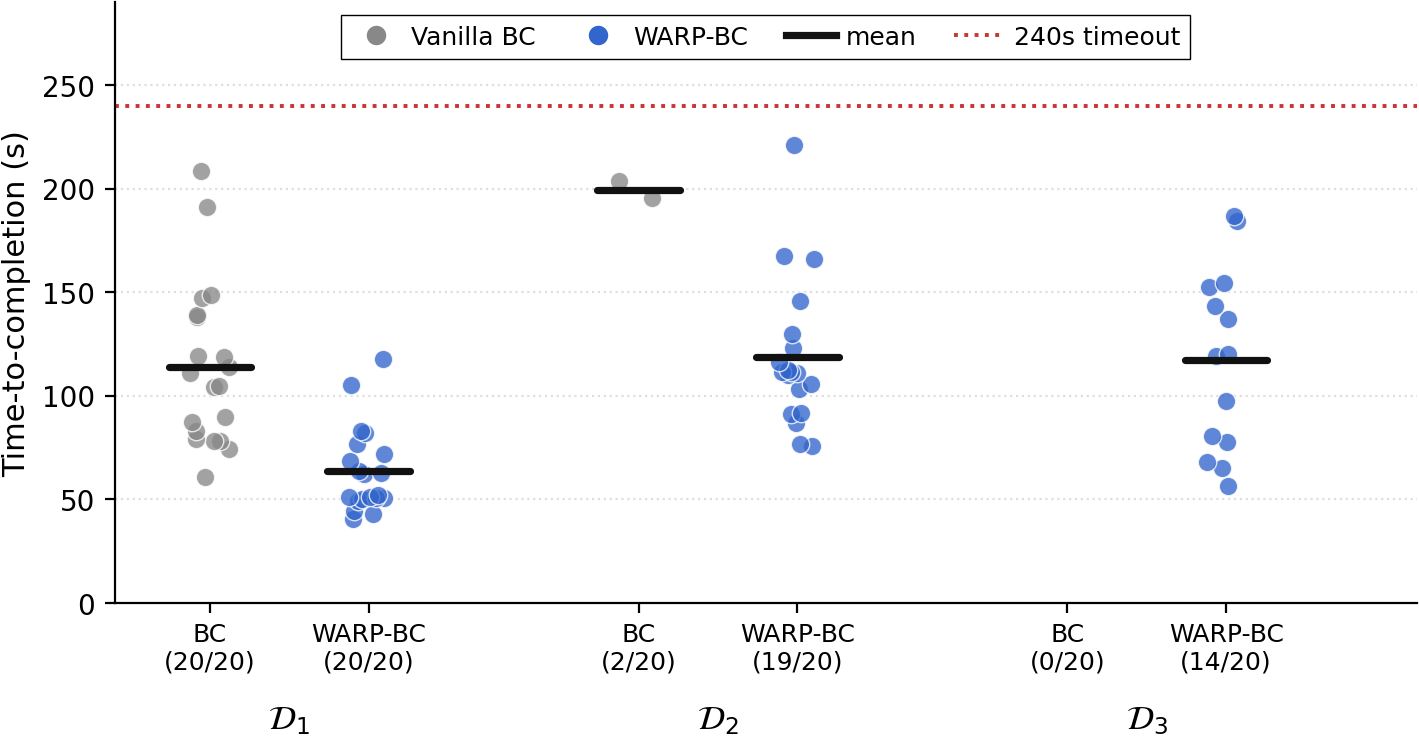
As shown in Table [tab:main95results] and Figure 4, while both methods succeed on \(\mathcal{D}_{1}\), WARP-BC yields a 1.78\(\times\) throughput improvement, with performance divergence increasing on \(\mathcal{D}_{2}\) (\(\sim18\times\) throughput improvement compared to vanilla BC) and \(\mathcal{D}_{3}\). From qualitative observation, vanilla BC on the later tiers often gets caught in repetitive, localized adjustments that fail to progress the task, often cycling through micro-adjustment behavior until the 240-second timeout is reached.
4.4 Baseline Comparisons↩︎
Because SARM requires human-annotated subtask boundaries, we evaluate all methods on augmented datasets \(\mathcal{D}_4 = \mathcal{D}_1 \cup \mathcal{D}_A\) and \(\mathcal{D}_5 = \mathcal{D}_2 \cup \mathcal{D}_A\), where \(\mathcal{D}_A\) provides annotated expert demonstrations (Table [tab:sarm95compare]). All other baselines treat \(\mathcal{D}_A\) as unlabeled data. Across methods, approaches retaining a larger fraction of action chunks degrade more substantially on \(\mathcal{D}_5\), whereas more selective curation strategies remain comparatively robust. SARM achieves 19/20 success on \(\mathcal{D}_4\) but drops to 2/20 on \(\mathcal{D}_5\). Relative to WARP-BC and DemInf, SARM retains a substantially larger fraction of action chunks (78.5% on \(\mathcal{D}_4\), 66.6% on \(\mathcal{D}_5\)), suggesting its filtering strategy may be insufficiently selective under broader training distributions. DemInf remains comparatively robust on \(\mathcal{D}_5\) (18/20 success) under a matched retained-data budget, though WARP-BC consistently achieves higher throughput across both tiers. SCIZOR performs well on \(\mathcal{D}_4\) (19/20 success) but drops to 2/20 on \(\mathcal{D}_5\). Similar to SARM, it retains a comparatively large fraction of action chunks (66.7% on \(\mathcal{D}_5\)), suggesting its temporal-distance proxy may provide weaker discrimination between efficient execution and localized hesitation behaviors in this setting. To see the distribution of time-to-completion times across methods on \(\mathcal{D}_4\) and \(\mathcal{D}_5\), see Appendix 10.
4.5 Ablations↩︎
2pt
| Ablations | Variant | Success | Mean TTC (s) | Thrput (/hr) | Act. Chunks Kept |
|---|---|---|---|---|---|
| Weighting | \(\tau = 0\) | 3/20 | 201.4 | 2.3 | 97.0% |
| \(\tau = 1\), binary | 16/20 | 139.6 | 18.0 | 34.4% | |
| \(\tau = 1\), continuous [WARP-BC] | 19/20 | 118.8 | 27.4 | 34.4% | |
| Aggregation | Mean \(\hat{v}\) over chunk | 15/20 | 127.0 | 17.4 | 34.0% |
| Mean \(\hat{v}\) over chunk, future offset | 14/20 | 124.2 | 15.9 | 34.3% | |
| Terminal \(\hat{v}_\text{end}\) [WARP-BC] | 19/20 | 118.8 | 27.4 | 34.4% | |
| Sampler | IID log-normal | 18/20 | 131.0 | 22.8 | 28.7% |
| AR(1) process [WARP-BC] | 19/20 | 118.8 | 27.4 | 34.4% |
Weighting Function. The binary and continuous \(\tau = 1\) variants utilize the identical threshold, meaning they retain the exact same 34.4% of action chunks. Yet, continuous weighting outperforms binary masking (19/20 vs. 16/20), demonstrating that continuous weighting scales the imitation loss proportionally to emphasize higher-progress execution segments. Aggregation Strategy. When summarizing frame-level velocities for an action chunk, gating by the terminal frame’s velocity \(\hat{v}_{\text{end}}\) (19/20) proves superior to both the aligned chunk mean (15/20) and a future-offset chunk mean (14/20). Mean aggregation—regardless of its temporal alignment—allows transient, high-velocity spikes to mask subsequent regressions within the same window. In contrast, terminal aggregation is designed to better isolate the boundaries of high-advantage segments. It biases retention towards the “leading edges" of task progress while providing a sharper cutoff for”trailing edges" that decelerate into hesitation. Time-Warp Sampler. We compare our smoothly correlated AR(1) sampler against an IID log-normal sampler. While the AR(1) process improves success marginally (19/20 vs. 18/20), it yields clearer gains in throughput. During inference, the model evaluates temporally continuous video streams likely characterized by smoother, natural variations in execution speed. The AR(1) process mimics this continuity during training. In contrast, IID sampling produces a more erratic distribution of frame gaps that may diverge from the downstream inference distribution on unseen demonstrations.
4.6 Bottle-in-Bin Placement Task↩︎
6pt
| Method | |||||
| Placed \(\uparrow\) | |||||
| Bottle (s) \(\downarrow\) | |||||
| (/hr) \(\uparrow\) | |||||
| Kept | |||||
| Vanilla BC | 59/80 | 15.9 | 147.8 | 100% | |
| WARP-BC | 74/80 | 11.3 | 237.8 | 30.6% |
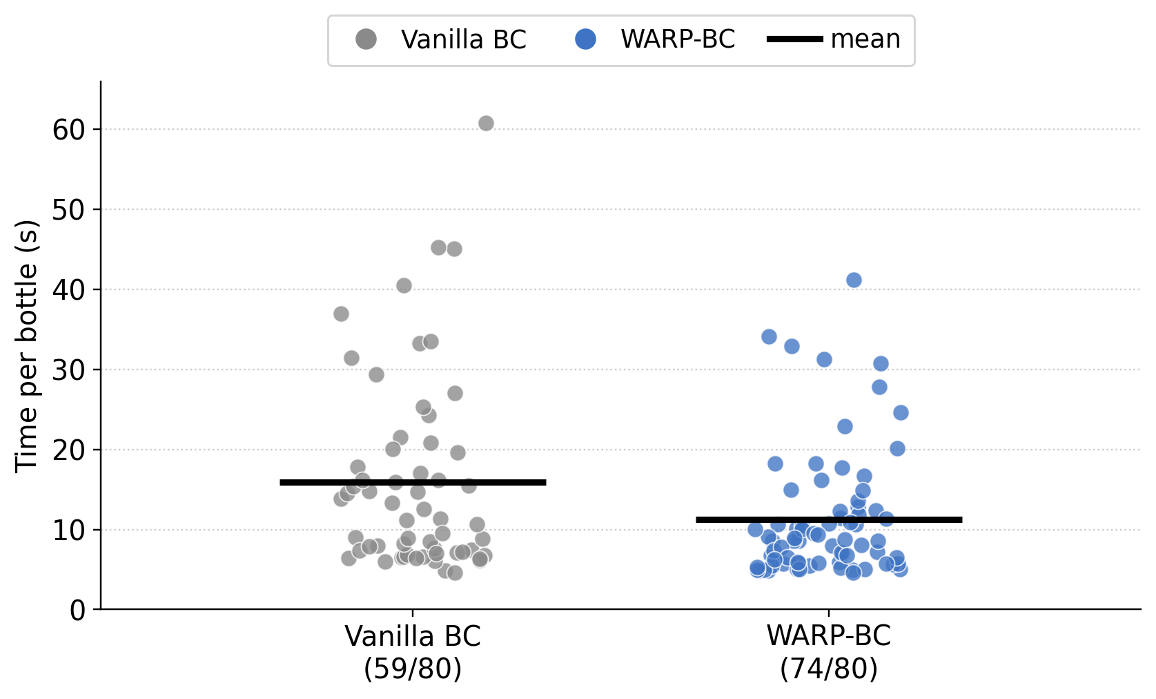
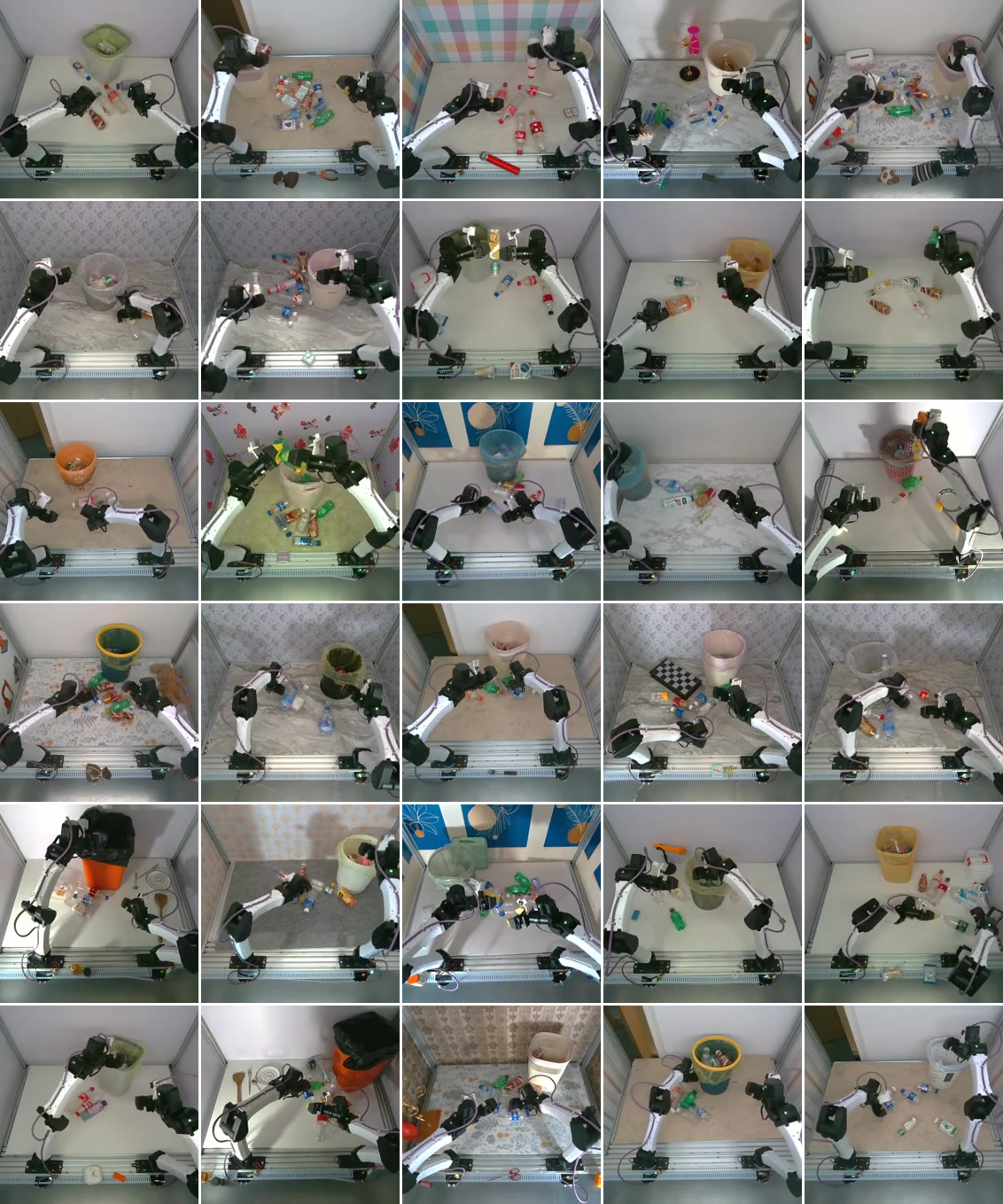
Beyond T-shirt folding, we evaluate WARP-BC on a bottle-in-bin placement task, where the robot places four plastic bottles into a bin (\(90\) s timeout, \(20\) trials per method). Both policies train on the same dataset of bottle demonstrations, and WARP-RM uses hyperparameters identical to the T-shirt setting (App. 7). Table 2 and Figure 5 show WARP-BC places \(74/80\) bottles versus \(59/80\) for vanilla BC, reducing mean per-bottle placement time from \(15.9\) to \(11.3\) s and improving throughput by \(1.6\times\) (\(237.8\) vs.\(147.8\) bottles/hr). Mean per-bottle placement time measures execution speed over successfully placed bottles only and is not penalized by missed bottles, whereas throughput charges each timed-out trial its full 90 s timeout and thus additionally reflects task completion. See App. 9 for evaluation-protocol details.
5 Limitations and Future Work↩︎
While WARP-BC attenuates the impact of suboptimal data, the resulting policy remains restricted to the behaviors present in the training set. Future work will investigate how post-training, e.g. DAgger, offline and online RL, and iterative self-improvement via reward-aligned learning, can generalize performance beyond these initial offline demonstrations. Furthermore, our experiments span two real manipulation tasks on a single bimanual embodiment, and several directions remain open. First, our negative-progress supervision comes entirely from reversed playback—an approximation we adopt from ReWiND [21], which notes that such reversals can be physically implausible. Whether this synthetic signal yields representations useful for downstream filtering and reweighting is not guaranteed, and we encourage practitioners to validate it on their own tasks. Second, the garment’s 2D image-space area may provide a strong implicit proxy for progress. Evaluating WARP-RM on tasks lacking such visual cues remains an important direction for future work.
6 Dataset Statistics↩︎
Table 3 reports per-tier statistics for the three policy training datasets used in Section 4, as well as the fixed reference subset on which WARP is trained. All tiers are length-filtered subsets of a single underlying dataset of human-teleoperated bimanual T-shirt-folding demonstrations. Figure 6 plots the corresponding episode-length distribution.
10pt
| Dataset / Tier | Description | Episodes | Total hours |
|---|---|---|---|
| \(\mathcal{D}_1\) | Policy training, length-filter \(\le 60\) s | \(2{,}427\) | \(36.1\) |
| \(\mathcal{D}_2\) | Policy training, length-filter \(\le 90\) s | \(4{,}124\) | \(71.3\) |
| \(\mathcal{D}_3\) | Policy training, length-filter \(\le 120\) s | \(6{,}473\) | \(139.7\) |
| \(\mathcal{D}_A\) | Annotated dataset, SARM train data | \(867\) | 13.9 |
| \(\mathcal{D}_{RM}\) | WARP-RM train data, \(\le 59.8\) s | \(1{,}950\) | \(28.7\) |
7 Bottle-in-Bin Dataset Statistics↩︎
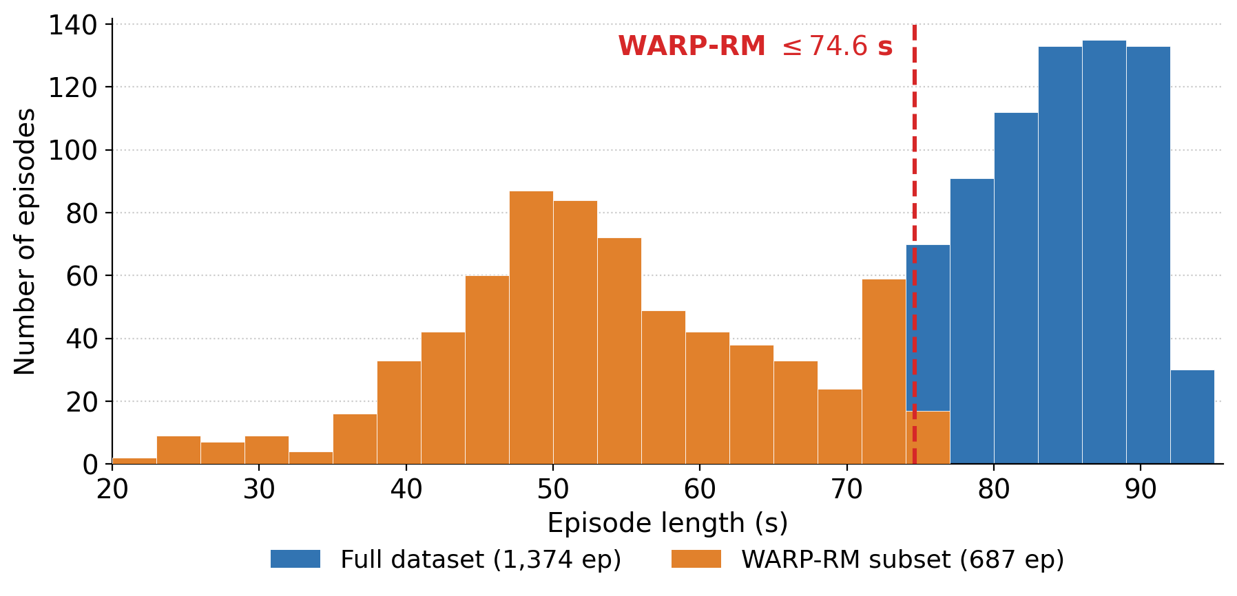
Table 4 and Figure 7 report dataset statistics for the bottle-in-bin placement task (Section 4, Table 2). Both the vanilla BC and WARP-BC policies are trained on the dataset of human-teleoperated “put the plastic bottles in the bin” demonstrations. As with the T-shirt dataset, WARP-RM is trained once on a fixed reference subset of the shortest demonstrations (\(\le 74.6\) s), providing a clean signal for the canonical execution pace (\(\hat{v} = 1\)). All WARP and WARP-RM hyperparameters are kept identical to the T-shirt setup (Tables 5–6); only the training dataset differs.
10pt
| Dataset | Description | Episodes | Total hours |
|---|---|---|---|
| Full dataset | Human-teleoperated demonstrations | \(1{,}374\) | \(26.4\) |
| WARP-RM subset | WARP-RM train data, shortest demos \(\le 74.6\) s | \(687\) | \(10.2\) |
8 Implementation Details↩︎
8.1 WARP Hyperparameters↩︎
6pt
| Group | Symbol / name | Value |
|---|---|---|
| Sampler (Eq. 1 –2 ) | Window length \(N\) | \(32\) frames |
| Canonical inter-token stride \(S\) | \(1.5\) s (45 frames @ \(30\) Hz) | |
| AR(1) autocorrelation \(\alpha\) | \(0.5\) | |
| Marginal log-velocity std \(\sigma_\infty\) | \(\ln 2\) | |
| Path-length mean \(\bar{s}\) | \(\mathrm{Uniform}([0.5,\; 2.5])\) seconds per gap | |
| Reversal rate \(\lambda_{\text{rev}}\) | \(1\) (Poisson) | |
| Global time-reverse prob.\(p_{\text{flip}}\) | \(0.5\) |
8.2 WARP-RM Hyperparameters↩︎
6pt
| Group | Symbol / name | Value |
|---|---|---|
| Targets (Eq. 3 ) | Framerate \(f\) | 30 Hz |
| Normalization \(C_{\text{norm}}\) | \((N{-}1)\cdot S \cdot f = 1395\) source-frames | |
| Output bins | \(30\), centers linearly spaced in \([-3, 3]\) | |
| Target encoding | two-hot | |
| Architecture | Visual backbone \(\phi\) | frozen DINOv3 ViT-B/16, \(768\)-dim |
| Input resolution | \(224 \times 224\) | |
| Temporal-diff projection | \(\mathbb{R}^{1536} \to \mathbb{R}^{768}\) (no bias) | |
| Encoder layers / heads / model dim | \(12\) / \(8\) / \(768\) | |
| Attention | bidirectional self-attention | |
| Dropout | \(0.15\) | |
| Positional embedding | fixed sinusoidal | |
| Optimization | Optimizer | AdamW (\(\beta_1{=}0.9\), \(\beta_2{=}0.999\)) |
| Peak learning rate | \(4 \times 10^{-4}\) (linear-scaled from \(10^{-4}\) at bs \(= 256\)) | |
| Weight decay | \(10^{-3}\) | |
| Batch size | \(1024\) windows | |
| Total steps | \(15\,000\) | |
| Warmup / schedule | \(1000\) linear warmup, cosine anneal to \(0\) | |
| Gradient clip | \(1.0\) |
8.3 WARP-BC Policy Training↩︎
We instantiate the behavior cloning policy with the \(\pi_0\) flow-matching backbone [2]. Action chunks span \(H = 30\) source-frames (\(1.0\) s); per-chunk weights \(w\) are precomputed once per episode using Eq. 4 with threshold \(\tau = 1.0\), and chunks with \(w = 0\) are removed from the dataset at construction time so they consume no compute. All other policy-side hyperparameters (optimizer, schedule, batch size, image augmentation) follow the public \(\pi_0\) recipe unchanged.
8.4 Dense Inference for Reweighting↩︎
To produce a per-frame velocity \(\hat{v}_t\) over a target policy training dataset, we run sliding-window inference at stride-\(1\) source-frame offsets, each window using the canonical \(S = 1.5\)s inter-token spacing. The \((N{-}1) \cdot S \cdot f\) overlapping per-window velocities covering source-frame \(t\) are averaged to give \(\hat{v}_t\). This is done once per episode before policy training begins; the resulting \(\hat{v}_t\) trace is cached alongside the dataset.
9 Evaluation Protocol Details↩︎
Trials in which the bin is knocked over (bottle task) or grasped instead of a garment within the first 10 seconds (folding task) are reset and repeated rather than scored, as the demonstrations contain no bin-recovery behavior. The same rule applies to all methods.
10 Additional Experimental Result Statistics↩︎
![Figure 8: Time-to-completion distribution for success across baseline comparisons. Evaluated on \mathcal{D}_4 = \mathcal{D}_1 \cup \mathcal{D}_A and \mathcal{D}_5 = \mathcal{D}_2 \cup \mathcal{D}_A. Policy rollouts which exceed 240 seconds are considered failures and are not shown. SCIZOR [34] successfully folds a T-shirt right before the 240 second timeout boundary on \mathcal{D}_5](/article/2606.28320/figures/assets/ttc_distribution_d4_d5.png "fig:")
11 WARP-RM Qualitative Results↩︎

12 Training Dataset Visual Diversity↩︎
References↩︎
At \(n=20\), single-trial success differences (e.g., 19/20 vs./20) fall within binomial sampling noise; only larger gaps should be read as meaningful. Where success rates are comparable, throughput and time-to-completion are more informative metrics.↩︎