Bridging Ab Initio Symmetries and Global Nuclear Masses with
Interpretable Neural Networks
June 26, 2026
Abstract
Ab initio modeling has established Wigner’s \(\rm SU(4)\) and Elliott’s \(\rm SU(3)\) as dominant symmetries of the nuclear force in light and intermediate-mass nuclei. We ask
whether they also govern nuclear binding across the entire chart. Our aim is not high-precision prediction but physical insight, through interpretable, symmetry-based models. From the \(\rm SU(3)\) and \(\rm SU(4)\) Casimir operators we construct three neural-network (NN) mass models: Feature-Informed NN (FINN) for point predictions, Gaussian-Informed NN (GINN) adding uncertainty quantification, and Wigner-Informed NN (WINN)—a
mass formula using the Casimirs as an operator basis. All are trained on AME2016 and validated on nuclei new to AME2020. The \(\rm SU(4)\) operators alone cut the root-mean-square error (RMSE) by
nearly half on train and test data, and by about a fifth on extrapolation, relative to the liquid-drop baseline—showing that Wigner’s symmetry carries predictive information beyond bulk properties. Despite its compact form, WINN reaches the lowest
validation RMSE, \(0.430\) MeV—competitive with state-of-the-art mass models—which we read less as a benchmark than as evidence that its symmetry basis captures important physics. WINN further reveals i) an enhancement of
the quadratic \(\rm SU(4)\) Casimir near the neutron dripline, signaling restoration of Wigner’s symmetry, and ii) an unexpected gain of the quartic operator in the superheavy region. We thereby elevate emergent symmetries
from the hidden order within individual nuclei to a governing principle of the whole nuclear chart.
Nuclear mass ,Machine learning ,Interpretable neural network ,Wigner’s SU(4) symmetry ,Elliott’s SU(3) symmetry
1 Introduction↩︎
Advances in computational hardware and data availability have catalyzed the adoption of machine learning (ML) in nuclear physics [1]. In particular, neural networks (NNs) have shown strong performance in modeling nuclear mass—a central quantity for \(r\)-process nucleosynthesis [2] and the composition of neutron star crusts [3]. Architectures explored to this end include light gradient boosting machine [4], mixture density network [5], fully connected NNs [6], decision trees [7], convolutional NN [8], Bayesian models [9]–[12], Gaussian processes and support vector regression [13], [14], as well as a hybrid between NN and density functional theory (DFT) [15].
The advantage of ML lies in its ability to capture recurring patterns that underpin physical systems. Atomic nuclei are particularly intriguing in this regard. Despite the complexity of the nuclear force, low-lying spectra are consistently dominated by two spatial symmetries: Elliott’s \(\rm SU(3)\) [16]–[18] and symplectic \(\rm Sp(3,R)\) [19] symmetries. Over the last two decades, ab initio nuclear theory has unveiled the dominance of these symmetries in light and intermediate-mass nuclei [20]–[23], leveraged them to model clustering phenomena and reactions [24], [25], and probed new physics beyond the Standard Model [26], [27].
Prior to the introduction of the \(\rm SU(3)\) symmetry, Wigner proposed the \(\rm SU(4)\) [or \(\rm U(4)\)] symmetry in 1937 [28], [29], for which he was awarded the Nobel Prize in 1963, alongside the pioneers of the nuclear shell model—Mayer [30], [31] and Jensen, Haxel and Suess [32]. Also known as the supermultiplet symmetry, it unifies the spin and isospin symmetries into a single framework. While the spin-orbit force breaking the symmetry in heavy nuclei casted doubt on the theory in the 1940s-50s, the 1960s saw renewed interest following the first observation of isobaric analog states in medium and heavy nuclei [33] and the formulation of a nuclear mass formula involving the second-order Casimir invariant of the \(\rm SU(4)\) group as a test of this symmetry [34], [35]. This model was later extended with higher-order Casimirs and shell corrections [36]–[38], exceeding the Bethe-Weizsäcker formula [39], which treats nuclei as liquid drops (LDM). Approaching its nine-decade milestone, Wigner’s symmetry has remained at the forefront of nuclear physics. First-principles studies recently establish \(\rm SU(4)\) as a dominant symmetry of the nuclear force, which arises naturally from the strong interaction in effective field theories [40], [41], is strongly manifested in light nuclei [42], [43], and governs the coupling of nuclear structure to the weak force [42]. These insights have been exploited to tame the sign problem of nuclear lattice simulations [44], [45] and to compress no-core shell-model spaces via the ab initio Symmetry Adapted Model (SAM) [43]. As with Elliott’s \(\rm SU(3)\), however, this evidence has been gathered mostly in light and intermediate-mass nuclei, where ab initio calculations are computationally tractable. In this paper, we take a deliberate leap by asking whether the \(\rm SU(3)\) and \(\rm SU(4)\) symmetries also govern binding across the nuclear landscape, well into regions of exotic isotopes, which are being synthesized beyond the dripline at frontier facilities like FRIB, TRIUMF, GSI, GANIL and potentially provide input for NASA’s Compton Spectrometer and Imager (COSI) mission [46], which is planned for launch in 2027. Traditionally, these emergent symmetries have guided the construction of the many-body basis of individual nuclei. Here we broaden their reach by turning the same symmetries, grounded in first principles, into a lens for probing and inferring nuclear systematics across the entire chart. We build a family of NN mass models—FINN, GINN, and WINN—from a compact set of features derived from the \(\rm SU(3)\) and \(\rm SU(4)\) Casimir invariants. The culmination is WINN, an interpretable bilinear formula whose eight symmetry-motivated terms reproduce known masses with a validation root-mean-square error (RMSE) of \(0.430\) MeV. This perspective opens new frontiers—the effectiveness of such a minimal symmetry basis invites broader extensions in both symmetry content and the range of observables for future work. The remainder of this paper is organized as follows. In Sec. 2, we describe how mass data are collected and split into train, test and validation sets, and introduce the symmetry-inspired features used in our models. Section 3 establishes the relevance of these features through two NNs, whose results inspire the interpretable mass formula presented in Sec. 4. Key findings and future directions are summarized in Sec. 5.
2 Data collection↩︎
2.1 Atomic mass datasets↩︎
We collect nuclear masses from two widely used datasets, namely AME2016 [47], [48] and AME2020 [49], [50], excluding those
extrapolated from theory. Following Refs. [4], [6], [13], we randomly split AME2016 into a train set (1908 nuclei) and a test set (478 nuclei) in an 80:20 ratio, and take the nuclei first reported in AME2020 as the
validation set (71 nuclei). Their roles are distinct: the train set fixes the network parameters; the test set, drawn from the same distribution but unseen during training, monitors overfitting (see Sec. S3 in Supplemental Material (SM) and Ref. [51]); and the validation set probes our NNs’ ability to predict completely unseen masses. We also exclude light nuclei (\(Z<8\) and \(N<8\)) from our calculations.
2.2 Symmetry-inspired features↩︎
In this work, we employ nine physics-informed features which are grouped into three categories.
LDM features—To describe bulk properties of nuclear binding, we consider features appearing in the LDM. The most conspicuous choices are the proton number \(Z\), which encodes Coulomb repulsion, and \(A^{2/3}\) for the surface energy. While one could include \(A\) for the volume term, we use the neutron number \(N\) instead, since \(A\) is perfectly colinear with \(N\) and \(Z\); choosing \(N\) and \(Z\) also lets the models somewhat resolve the neutron and proton shell closures. Finally, we include \(T_z = (N-Z)/2\) to capture the asymmetry of the nuclear chart.
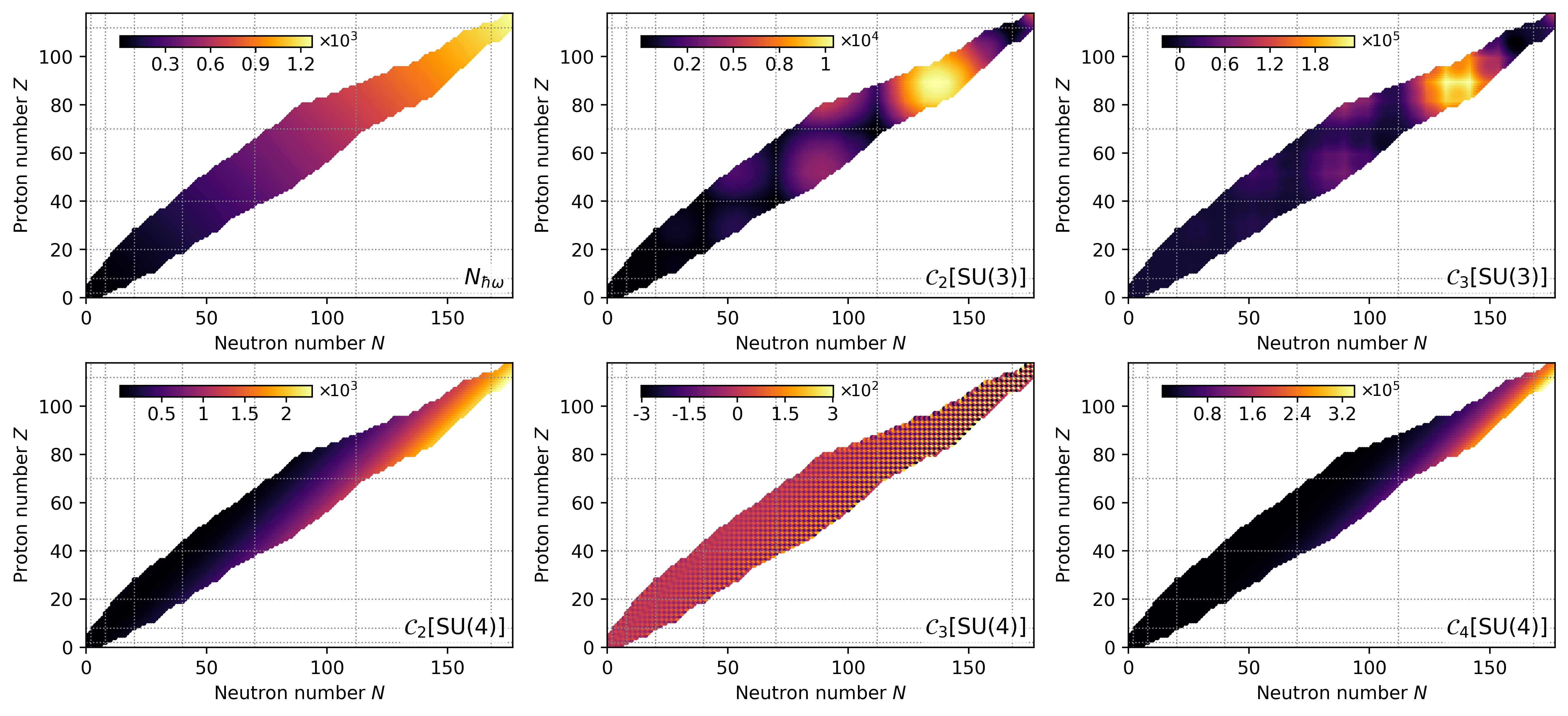
SU(4) features—Inspired by former works [36]–[38], we consider the \(\rm SU(4)\) Casimir operators (see Sec. S1 in SM and Refs. [52]–[56]) to be features. These include the two-, three- and four-body operators, \(\mathcal{C}_2\), \(\mathcal{C}_3\) and \(\mathcal{C}_4\), that describe spin-isospin polarization forces. Since these operators depend on \(\rm SU(4)\) irreducible representations (irreps) and several irreps are allowed for a given nucleus, we hypothesize that the preference toward the lowest-\(\mathcal{C}_2\) irrep revealed by the SAM’s first-principles calculations for light nuclei [43] also extends to the entire nuclear chart. Figure 1 shows evolution of these operators. While the quadratic and quartic operators gradually increase for heavier nuclei, the cubic Casimir exhibits a sign fluctuation between odd-mass nuclei, which becomes increasingly pronounced for very neutron-rich isotopes.
SU(3) features—We select three features stemming from the three-dimensional harmonic oscillator (3DHO) shells. One is the number operator \(N_{\hbar\omega}\) that counts the total number of oscillator quanta of a particular distribution of nucleons across the shells. The others are the second- and third-order invariants of the \(\rm SU(3)\) group (see Sec. S2 in SM and Ref. [57]). The former, \(\mathcal{C}_2\), signifies the magnitude of the mass quadrupole moment, whereas the latter, \(\mathcal{C}_3\), indicates whether the nucleus is spherical (zero), prolate (positive), or oblate (negative) [58], [59]. For each nucleus, an \(\rm SU(3)\) irrep is selected such that it combines antisymmetrically with the \(\rm SU(4)\) irrep and maximizes deformation [21]. Across the chart, these operators peak at mid-shells where nuclei tend to deform and get suppressed at shell closures where nuclei are mostly spherical (Fig. 1).
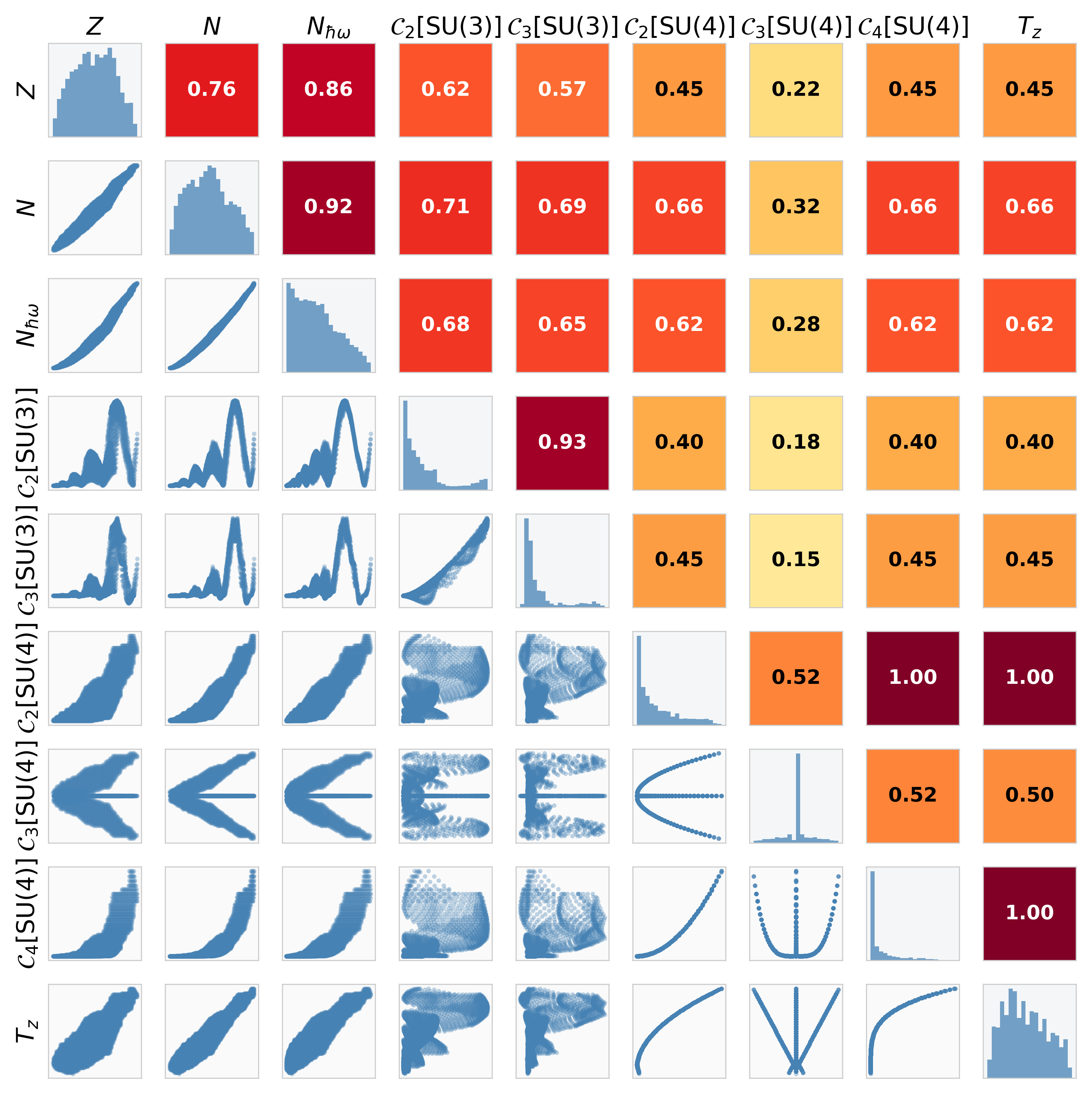
Feature correlations—Before training our models, we examine the pairwise relationships among the features. As the scatter plots in Fig. 2 show, these relationships are predominantly non-monotonic; hence, we quantify them with the maximal information coefficient (MIC) [60], which captures both linear and nonlinear dependence, rather than the Pearson or Spearman coefficients [61]. First, \(N_{\hbar\omega}\) is strongly correlated with \(N\) and \(Z\) (MIC \(\approx 0.9\)), indicating that it largely tracks the mass number \(A\), consistent with its evolution in Fig. 1. Second, the \(\rm SU(3)\) invariants are tightly coupled to each other (MIC \(=0.93\)), as both encode quadrupole collectivity, while sharing only moderate information with the bulk features (MIC \(\approx 0.6\)-\(0.7\)). Third, the even \(\rm SU(4)\) Casimirs (\(\mathcal{C}_2\) and \(\mathcal{C}_4\)) are perfectly correlated with \(T_z\) (MIC \(=1.00\)). That means, for the dominant irrep, their eigenvalues reduce to smooth even functions of \(T_z\) (see Sec. S1 in SM), implying that \(\mathcal{C}_2\) and \(\mathcal{C}_4\) add no statistical information beyond the isospin asymmetry. However, their role is to supply the specific power functions of \(T_z\) that embody the supermultiplet structure as a physically motivated inductive bias. Fourth, \(\mathcal{C}_3[\rm SU(4)]\) is weakly correlated with every other feature (MIC \(\leq 0.32\) with the bulk and \(\rm SU(3)\) sectors1), reflecting the sign fluctuation noted above. Section S6 in SM demonstrates that \(\mathcal{C}_3[\rm SU(4)]\) is an irrelevant feature and is excluded henceforth.
| Feature set | FINN | GINN | WINN | ||||||||
| Train | Test | Validation | Train | Test | Validation | Train | Test | Validation | |||
| LDM | 0.944 | 1.111 | 1.270 | 0.869 | 1.149 | 1.304 | |||||
| LDM+SU(4) | 0.521 | 0.588 | 1.024 | 0.604 | 0.654 | 1.046 | |||||
| LDM+SU(3) | 0.915 | 1.306 | 1.603 | 1.036 | 1.404 | 1.280 | |||||
| LDM+SU(4)+SU(3) | 0.411 | 0.552 | 0.624 | 0.400 | 0.488 | 0.793 | 0.400 | 0.447 | 0.430 | ||
3 Symmetry-informed neural networks↩︎
3.1 Architecture↩︎
We first employ two NN architectures, which learn a direct functional map \(\mathbf{y} = \mathcal{F}(\mathbf{x})\) from features to binding energy, to determine whether the symmetry features are relevant for nuclear binding. This is carried out by testing four combinations of features (Table 1): the LDM baseline, and the LDM augmented with SU(3) and/or SU(4) features. If the symmetry features are indeed important, one must see improvement on RMSE across the train, test and validation datasets.
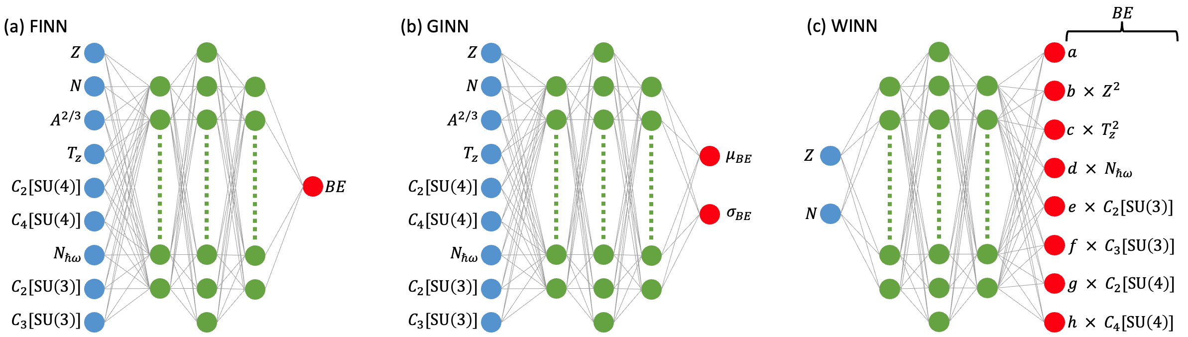
The two NNs are i) a single-output NN (called FINN for Feature-Informed NN) that treats binding energy (\(BE\)) as an absolute output [Fig. 3 (a)], ii) a two-output NN (called GINN for Gaussian-Informed NN) that models \(BE\) as a statistical variable with expectation value (\(\mu_{BE}\)) and uncertainty (\(\sigma_{BE}\)) [Fig. 3 (b)]. The loss function subsumes two terms, \(\mathcal{L} = \mathcal{L}_0 + \lambda \mathcal{L}_1\) with the weight \(\lambda\) chosen to be \(2.0\) for the FINN and \(4.0\) for the GINN. Here, \(\mathcal{L}_0\) is an architecture-based loss, i.e., the mean-squared error (MSE) for the FINN and the negative log-likelihood (NLL) loss [\(\langle (BE - \mu_{BE})^2/2\sigma_{BE}^2 + \log \sigma_{BE} \rangle\)] for the GINN; \(\mathcal{L}_1\) is a physics-informed loss adapted from Refs. [5], [13], [62] and based on the Garvey-Kelson (GK) relations [63].
Both the NNs are trained on mini batches of size 64 for 2000 epochs; at every mini-batch step, \(\mathcal{L}_1\) is evaluated on the whole train set. We also use the SOAP optimizer [64], a second-order method with learning rate of \(10^{-3}\) that we find outperforms the Adam optimizer [65] on the validation benchmark. To facilitate learning, all features and target \(BE\) are standardized to zero mean and unit variance as
described in Sec. S4 of SM.
3.2 Results and interpretation↩︎
Table 1 reports the NN’s performance across four feature sets. For the FINN, the LDM baseline with only the macroscopic inputs \((Z, N, A^{2/3}, T_z)\) achieves a validation RMSE of \(1.270\) MeV, consistent with the inherent limitation of a purely bulk description. Adding the \(\rm SU(4)\) Casimirs reduces the error sharply—by nearly half on the train and test sets and by about a fifth on validation (to \(1.024\) MeV)—demonstrating that Wigner’s symmetry carries substantial predictive information beyond the liquid-drop terms. Expanding the feature set further with the \(\rm SU(3)\) invariants yields the best result, \(0.624\) MeV on the validation set. By contrast, the \(\rm SU(3)\) features alone on top of the LDM do not improve the validation error (\(1.603\) MeV), confirming that \(\rm SU(4)\) is the dominant contributor [66] and that \(\rm SU(3)\) becomes beneficial only in combination with it.
The GINN follows a similar trend with respect to feature richness. The full feature set continues to achieve the lowest validation RMSE (\(0.793\) MeV). Moreover, by examining the uncertainty \(\sigma_{BE}\) across the nuclear chart (Fig. 4), one can infer the confidence of the model. With the LDM features, the model is more confident for heavy nuclei that behave mostly like a fluid and displays a lack of confidence for intermediate-mass nuclei where microscopic effects are important, which are addressed by the \(\rm SU(3)\) features. The \(\rm SU(4)\) features increase confidence broadly across the chart with the most notable improvement for exotic isotopes near the driplines.
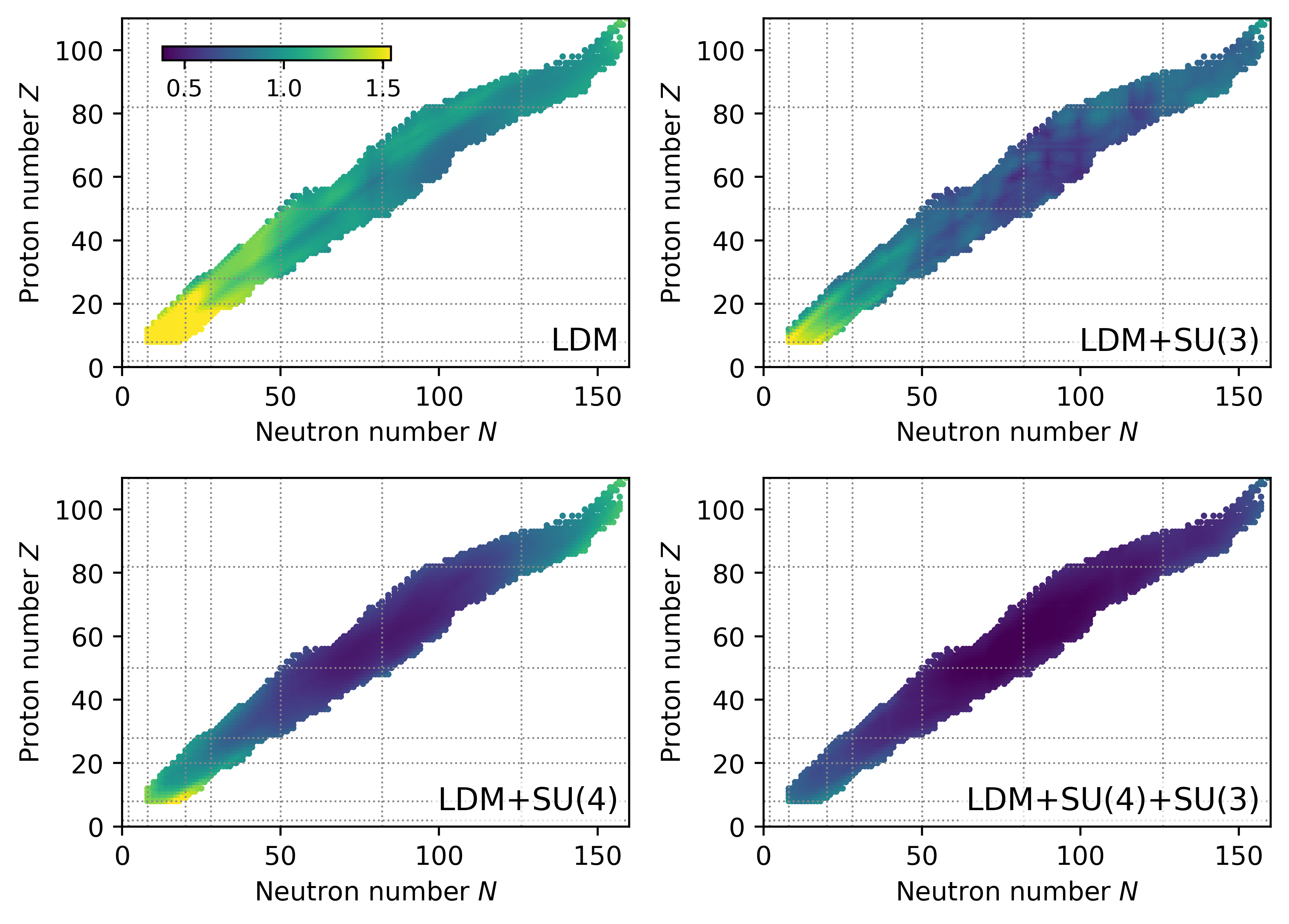
On all datasets, the FINN attains a lower RMSE than the GINN for most cases (Table 1). This systematic offset is structural: in the NLL loss the gradient on \(\mu_{BE}\) is weighted by \(1/\sigma_{BE}^2\), thus the network can lower the loss by inflating \(\sigma_{BE}\), trading point accuracy for wider intervals. To counter this, we enlarge \(\lambda\) to \(4.0\) for a stronger constraint and adopt the \(\beta\)-NLL weighting [67] that rescales each loss by a stop-gradient factor \(\sigma_{BE}^{2\beta}\) with \(\beta = 0.5\) to tighten point accuracy. The FINN, minimizing the MSE directly, is immune to this trade-off and tends to retain an RMSE edge. Nonetheless, the GINN’s value lies not in point accuracy but in the calibrated per-nucleus uncertainty \(\sigma_{BE}\) (Fig. 4), which the FINN cannot supply.
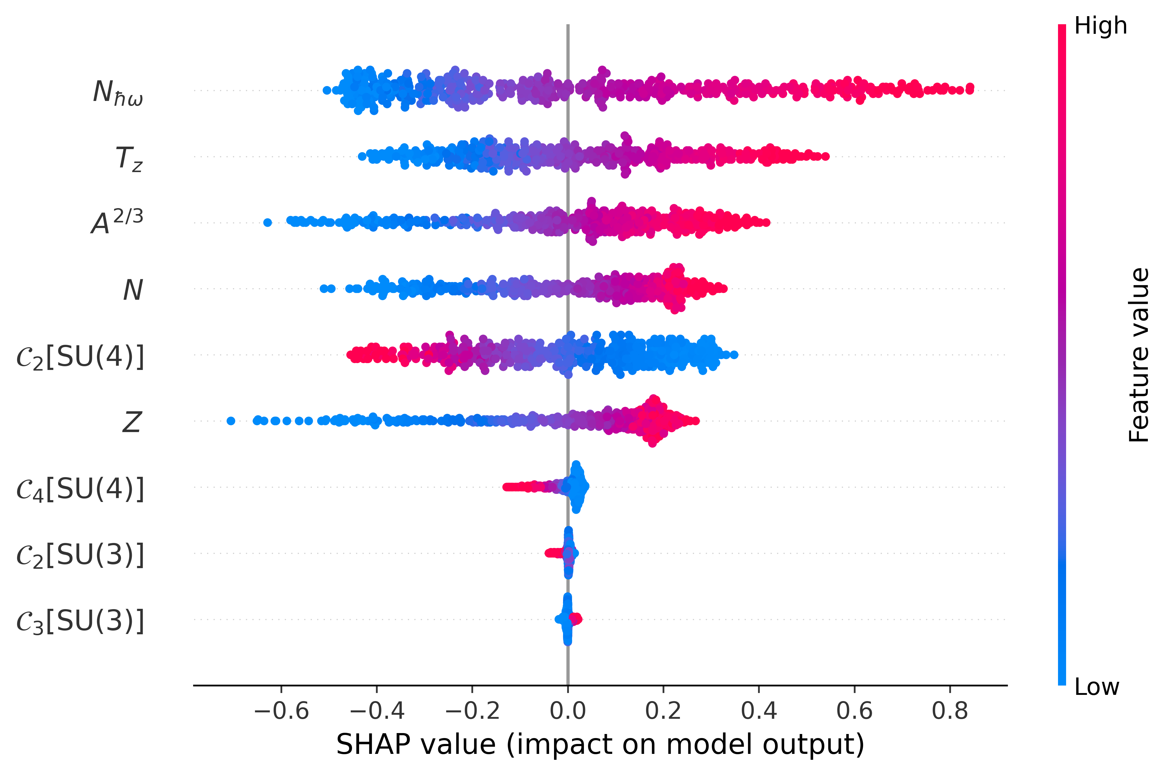
We also probe feature influence using the Shapley additive explanations (SHAP) values [68]. The summary plot for the full-set GINN (Fig. 5) confirms that nuclear masses are primarily driven by the bulk LDM features. Notably, \(N_{\hbar\omega}\) ranks unexpectedly high—comparable to the LDM ones—likely because it grows monotonically across the chart (Fig. 1) and correlates strongly with \(N\) and \(Z\) (Fig. 2), acting as a proxy for the omitted mass number \(A\). In addition, we witness that the \(\rm SU(4)\) features outrank the \(\rm SU(3)\) ones, consistent with the results in Table 1 and Fig. 4.
4 An interpretable symmetry-informed neural network↩︎
4.1 Architecture↩︎
While the NNs of the preceding section establish the relevance of the symmetry features, they obscure how each feature shapes binding across different regions of the nuclear landscape. Motivated by those results and earlier works [36], [38], we propose a four-body bilinear mass formula, \[\begin{align} \label{WINN} BE = a & + b Z^2 + c T_z^2 + d N_{\hbar\omega} + e \mathcal{C}_2 [{\rm SU(3)}] \nonumber\\ & + f \mathcal{C}_3 [{\rm SU(3)}] + g \mathcal{C}_2 [{\rm SU(4)}] + h \mathcal{C}_4 [{\rm SU(4)}], \end{align}\tag{1}\] where the coupling strengths \(\{a,b,c,d,e,f,g,h\}\) are functions of \(N\) and \(Z\). The role of \(a\) is to include the “leftover” of nuclear binding beyond the symmetry descriptors. As mentioned in the correlation analysis (Sec. 2.2), for the leading irrep, the even \(\rm SU(4)\) Casimirs reduce to smooth functions of \(|T_z|\); therefore, adding them on top of \(T_z^2\) allows the model to learn the physics associated with the widely known Wigner energy [69]. We design a NN, termed WINN (Wigner-Informed NN), to learn the evolution of the coupling strengths across the nuclear chart [Fig. 3 (c)]. The WINN is trained with a loss similar to the FINN, but with only 1000 epochs and weight decay of \(0.01\) to prevent overfitting. We also find that the GK weight must be set much smaller for the WINN (\(\lambda = 0.15\)) than for the other two architectures. This weight controls how strongly the model is penalized for violating local nuclear-chart consistency. For the FINN and GINN, which have no built-in knowledge of how \(BE\) scales with \(N\) and \(Z\), a large weight is essential to enforce this locality. For the WINN, the operator basis already encodes this regularity, so the GK term acts as a lightweight refinement rather than a structural constraint, and a small weight suffices.
4.2 Results and interpretation↩︎
The WINN’s performance is summarized in Table 1. This guided approach surpasses the other NNs: it not only achieves the best validation RMSE (\(0.430\) MeV) but also maintains an excellent balance across the train, test, and validation sets. Notably, with only eight operators, the WINN is comparable with other modern mass models, see Table 3 in Ref. [4]. We also find that the pairing effect is captured without an explicit term: the \(BE\) residuals exhibit no systematic sign inversion between even-even and odd-odd nuclei and no staggering for odd-\(A\) isotopes (see Sec. S7 in SM).
To assess WINN’s predictive capability beyond the known isotopes, we compare its \(BE\) predictions against two well-established mass models: the macroscopic-microscopic WS3 model [70] and the fully microscopic Hartree-Fock-Bogoliubov model HFB-26 [71], evaluated on almost 6000 nuclei that each model predicts to be bound beyond those in AME2020. This comparison is asymmetric by construction: both reference models are global fits with dozens of parameters,
whereas WINN relies on a bilinear formula with only eight symmetry operators. Stratifying the comparison by distance from the AME2020 boundary within each isotopic chain, we find good agreement near the known region: for nuclei within 5
neutrons of the last measured isotopes, WINN matches WS3 (HFB-26) within 5 MeV for \(78\%\) (\(71\%\)) of cases, with a mean absolute deviation (MAD) of \(3.6\) (\(4.6\)) MeV. Agreement degrades systematically deeper into unexplored territory, the MAD rising to \(6.0\) (\(6.9\)) MeV
at 5-10 neutrons, \(10.5\) (\(11.1\)) MeV at 10-20 neutrons, and \(26\) (\(24\)) MeV beyond 20 neutrons from the last known
nuclei. The near-identical trends against two independent models confirm that this degradation reflects the genuine limits of extrapolating a compact eight-term model. We regard the near-boundary performance as encouraging evidence that the \(\rm SU(3)\otimes SU(4)\) operator basis captures the dominant physics up to roughly 10 neutrons from the known chart. Reliable WINN predictions deeper into terra incognita will require extending Eq. (1 )
with additional operators or incorporating microscopic inputs beyond the current work.

As noted above, the purpose of the WINN is to expose the role that each feature plays across the chart of nuclides. By analyzing the fractional contribution (Fig. 6) of each term in Eq. (1 ), we observe that \(a\) is the primary driver of nuclear binding, accounting for more than 45% of the mass for all nuclei, followed by \(N_{\hbar\omega}\) at about 25-50% level. The term \(Z^2\) mimics Coulomb energy, lowering \(BE\) on the neutron-deficient side, whereas the term \(T_z^2\) becomes vital toward the neutron dripline and in superheavy elements.
The model also successfully learns the shell structure encoded in the \(\rm SU(3)\) Casimirs. Near shell closures, where deformation is low, \(BE\) is largely unaffected by these two operators; at mid-shell, \(\mathcal{C}_2\) lowers the masses by a few percent while \(\mathcal{C}_3\) contributes less than 1%. Moreover, the signs of these coupling strengths are consistent with those determined from spectra of \(\alpha\)-like nuclei in Refs. [72], [73].
Lastly, the \(\rm SU(4)\) Casimirs exhibit two notable behaviors. The quadratic \(\mathcal{C}_2\) contributes at the few-percent level across most of the nuclear chart; however, a pronounced enhancement—reaching about 10-40% of \(BE\) and competing with the shell-driven \(N_{\hbar\omega}\)—emerges near the neutron dripline in the region \(Z \approx\) 8-60. This behavior points to the long-held expectation that Wigner’s symmetry is restored in neutron-rich isotopes [35], [37] due to the suppression of the spin-orbit splitting [74]–[76]. (The degree of \(\rm SU(4)\) restoration has been assessed for calcium isotopes [77] and more recently for heavy and superheavy nuclei through Gamow-Teller resonances [78].) A similar dripline enhancement is observed for the fourth-order Casimir, though roughly an order of magnitude smaller. Interestingly, \(\mathcal{C}_4\) gains substantial strength in the superheavy region (\(N \gtrsim 126\)), becoming competitive with \(\mathcal{C}_2\). Since \(\mathcal{C}_4\) is a four-body operator sensitive to quartet spin-isospin correlations, it might be worth investigating the microscopic origin of this amplification and its connection to the dominance of \(\alpha\)-systematics in this regime.
5 Summary and future outlooks↩︎
We have presented three symmetry-informed NN mass models built on the Casimir operators of Wigner’s \(\rm SU(4)\) and Elliott’s \(\rm SU(3)\) symmetries, trained on AME2016
and validated on nuclei first reported in AME2020 as a genuine test of extrapolation. The \(\rm SU(4)\) Casimirs alone reduce RMSE by nearly half on the train and test sets and by about a fifth on validation
relative to the LDM baseline; and the SHAP analysis ranks the \(\rm SU(4)\) features above the \(\rm SU(3)\) ones, establishing Wigner’s symmetry as the dominant microscopic contributor
beyond bulk properties [66]. Combining both sectors yields validation RMSEs of \(0.624\) and \(0.793\) MeV for the FINN and GINN, while the eight-term WINN does best at \(0.430\) MeV—evidence that embedding physics directly in the architecture is more effective than supplying it as input
features alone. We emphasize that high-precision mass prediction was never our goal: WINN’s competitive RMSE matters less as a benchmark than as proof that a compact symmetry basis encodes essential physics. The WINN coupling strengths further illuminate
the physics of different mass regions. The \(\rm SU(3)\) Casimirs capture deformation-driven shell effects, peaking at mid-shell and suppressed at shell closures. The quadratic \(\rm SU(4)\)
Casimir is enhanced near the neutron dripline (\(Z \approx\) 8-60), which we associate with the restoration of Wigner’s symmetry under spin-orbit quenching. The significant rise of the quartic Casimir \(\mathcal{C}_4[\rm SU(4)]\) in the neutron-rich superheavy region, where \(\alpha\)-systematics becomes dominant, warrants a dedicated study and will be pursued in follow-up work.
We highlight that, throughout this work, the \(\rm SU(3)\) and \(\rm SU(4)\) symmetries are assumed to hold exactly across the chart, with irrep selection inspired by ab initio results. In reality they are broken, a difficulty that has historically been addressed through pseudo and proxy schemes [79]–[84]. Our results carry a two-fold implication: i) the traditional algebraic solutions may improve the NNs through better choices of irreps, and ii) the NN architecture may itself offer a pathway for resolving the symmetry breaking, owing to its capacity to absorb the associated nonlinearities. Both possibilities will be explored in future work.
Finally, beyond the novel results, this work opens a new door in how we engage the emergent symmetries of the nuclear force. Where they once organized the structure of individual nuclei, ML now lets them speak to the systematics of the global nuclear landscape. In particular, extending the framework to other observables, e.g., \(\beta\)-decay, is a natural step toward a data-driven, symmetry-informed description of nuclear structure.
Declaration of competing interest↩︎
The authors declare that they have no known competing financial interests or personal relationships that could have appeared to influence the work reported in this paper.
Acknowledgements↩︎
We thank the LSU AI journal club for facilitating collaboration. This work was supported by LSU Sponsored Research Rebate Program and LSU Foundation’s Distinguished Research Professorship Program. PD acknowledges support from the Quad Fellowship of the Institute of International Education and the LSU Physics & Astronomy Department. A part of the work of FP was supported by the National Natural Science Foundation of China under Grant No. 12175097.
Data availability↩︎
The code used to construct the features, train the neural-network models, and reproduce results and figures of this work, together with data supporting our findings, is publicly available on this GitHub repository. We invite interested researchers and students to contribute and enrich the project.
Declaration of generative AI usage↩︎
During the preparation of this manuscript the author(s) used Claude by Anthropic and Prism by OpenAI in order to polish sentences and enhance coherence of the article. After using this tool/service, the author(s) reviewed thoroughly and edited the content as needed and take(s) full responsibility for the content of the published article.
Supplemental Material
6 Eigenvalues of SU(4) Casimir invariants↩︎
Explicit formulas for the Casimir invariants (\(\mathcal{C}_2\), \(\mathcal{C}_3\) and \(\mathcal{C}_4\)) of the \(\rm SU(4)\) group were derived for Wigner’s convention of \(\rm SU(4)\) labels by Burdet, Maguin and Partensky [52], and by Danos and Gillet [53]. In this work, we adopt an alternative convention of \(\rm SU(4)\) irreps by Draayer [54], \[P = n_{14}-n_{24} \text{, } P' = n_{24} - n_{34} \text{ and } P'' = n_{34} - n_{44},\] where \([n_{14}, n_{24}, n_{34}, n_{44}]\) is a \(\rm U(4)\) irrep [56] that sums up to the total number of nucleons, i.e., \(A=\sum_{i=1}^4 n_{i4}\).
The eigenvalues of the Casimir operators are derived following a general technique presented in Appendix B of Ref. [55] and applicable to any unitary group. Since the Casimir invariants only depend on the irrep labels, their eigenvalues can be computed in any subgroup chain that is most convenient, which we choose to be the canonical chain \(\rm U(4) \supset U(3) \supset U(2) \supset U(1)\). The \(\rm U(4)\) Casimir operators are defined in terms of the canonical generators \(E_{ij}\) [56] as follows \[\begin{align} \label{eq:U495Casimir} \mathfrak{C}_2 = E_{ij} E_{ji} \text{, } \mathfrak{C}_3 = E_{ij} E_{jk} E_{ki} \text{ and } \mathfrak{C}_4 = E_{ij} E_{jk} E_{kl} E_{li}, \end{align}\tag{2}\] where summations over double indices are implied according to Einstein’s convention. Another property of the Casimirs is their independence from any state used to evaluate the eigenvalue; hence, we choose the highest weight state that enables automatic annihilation of half of the terms in Eqs. (2 ). Once the eigenvalues of the \(\rm U(4)\) invariants are attained, those of the \(\rm SU(4)\) Casimirs are straightforward by a simple conversion from \(\rm U(4)\) to \(\rm SU(4)\) quantum numbers [55]. One last step is to invoke a linear mapping that preserves their algebraic properties \[\mathcal{C}_2 = 2 \mathfrak{C}_2 \text{, } \mathcal{C}_3 = 4(\mathfrak{C}_3 - \mathcal{C}_2) \text{ and } \mathcal{C}_4 = \mathfrak{C}_4 - \mathcal{C}_3,\] so that the following symmetry relations for the Casimirs under irrep conjugation are satisfied \[\begin{align} \mathcal{C}_2(PP'P'') = \mathcal{C}_2(P''P'P) \text{, } \mathcal{C}_3(PP'P'') = -\mathcal{C}_3(P''P'P) \text{ and } \mathcal{C}_4(PP'P'') = \mathcal{C}_4(P''P'P). \end{align}\]
Using the matrix elements given in Ref. [56], we arrive at the following expression for the Casimirs’ eigenvalues \[\begin{align} \langle \mathcal{C}_2 \rangle =& \frac{3}{2}(P^2+P''^2) + 2P'^2 + 2(P+P'') P' + P P'' + 6(P + P'') + 8P', \\ \langle \mathcal{C}_3 \rangle =& \frac{3}{2} (P - P'')[P^2 + P''^2 + 2(P P' + P' P'' + P P'') + 2(3P + 2P' + 3P'' + 4)], \\ \langle \mathcal{C}_4 \rangle =& \frac{1}{64} [21(P^4 + P''^4) + 16 P'^4 + 4P^3 (14 P' + 7 P'' + 42) + 4 P''^3 (14 P' + 7 P + 42) \nonumber \\ & + 32 P'^3 (4 + P + P'') + 72 P'^2 (P^2 + P''^2) + 30 P^2 P''^2 + 24 P P' P'' (3 P + 2 P' + 3 P'') \nonumber \\ & + (288 P'^2 + 896 P' + 960) (P + P'') + 24 P^2 (16 P' + 9 P'') + 24 P''^2 (16 P' + 9 P) \nonumber \\ & + 384 P P' P'' + 576 (P^2 + P''^2) + 512 P'^2 + 640 P P'' + 1024 P' ]. \end{align}\]
For the dominant lowest-\(\mathcal{C}_2\) irrep adopted throughout this work, the labels \((PP'P'')\) according to Draayer’s convention [54] are fixed by proton and neutron numbers, thus the even Casimirs reduce to smooth even functions of the isospin projection \(T_z=(N-Z)/2\), which is consistent with their correlation coefficient (MIC) with \(T_z\) shown in Fig. 2 of the main text. Note that explicit determination of the leading \(\rm SU(4)\) irrep analytically from \(T_z\) is provided in Refs. [37], [38]; however, we did not adopt these formulas since there are different conventions of the \(\rm SU(4)\) labels and it is not clear which convention these references followed. We instead construct a Python code to obtain the \(\rm U(4)\), then \(\rm SU(4)\), irrep for each nucleus that can decompose to \(T_z\) [56] and has the lowest \(\mathcal{C}_2\); in this way, we can conveniently determine the \(\rm U(3)\) irrep and its \(\rm SU(3)\) reduction as well. It is very much possible that subleading irreps would not be constrained by \(N\) and \(Z\) in the same way, i.e., their Casimir eigenvalues are no longer smooth functions of \(T_z\), which we will investigate in future work.
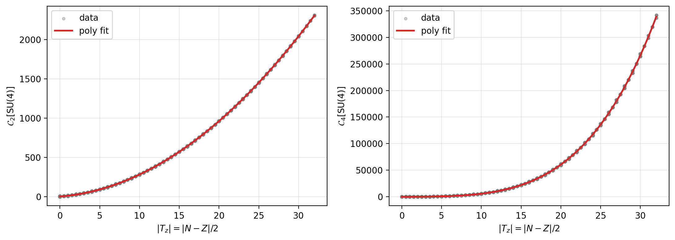
Since \(\mathcal{C}_2\) and \(\mathcal{C}_4\) are quadratic and quartic in their degree and are always non-negative, we fit their values against \(|T_z|\) to detect their dependence exactly (Fig. 7). Our polynomial fit yields the following results \[\begin{align} \langle \mathcal{C}_2 \rangle &\simeq 2.00\,|T_z|^2 + 7.97\,|T_z| + 3.20, & (R^2 = 0.99998), \\ \langle \mathcal{C}_4 \rangle &\simeq 0.25\,|T_z|^4 + 1.90\,|T_z|^3 + 11.9\,|T_z|^2 + 15.5\,|T_z| + 22.9, & (R^2 = 0.99991) \end{align}\] where \(R^2\) is the coefficient of determination. Crucially, the linear \(|T_z| \propto |N-Z|\) term in both \(\mathcal{C}_2\) and \(\mathcal{C}_4\) represents the Wigner energy [69], which is known as the cusp at \(N=Z\). Therefore, the inclusion of \(\mathcal{C}_2\) on top of \(T_z^2\) in the WINN mass formula is equivalent to adding the Wigner energy, whereas \(\mathcal{C}_4\) brings in higher orders of isospin asymmetry.
7 Eigenvalues of SU(3) Casimir invariants↩︎
We follow the convention for the eigenvalues of the quadratic (\(\mathcal{C}_2\)) and cubic (\(\mathcal{C}_3\)) Casimir operators belonging to the \(\rm SU(3)\) group by Draayer and Rosensteel [57], which can be derived similarly to those of the \(\rm SU(4)\) group and are given as \[\begin{align} \langle \mathcal{C}_2 \rangle &= \lambda^2 + \mu^2 + \lambda\mu + 3\lambda + 3\mu, \\ \langle \mathcal{C}_3 \rangle &=\frac{1}{9} (\lambda -\mu)[2\lambda^2 + 2\mu^2 + 5\lambda\mu + 9(\lambda + \mu + 1)]. \end{align}\] These operators satisfy the following property under irrep conjugation \[\begin{align} \mathcal{C}_2(\lambda\mu) = \mathcal{C}_2(\mu\lambda) \text{ and } \mathcal{C}_3(\lambda\mu) = - \mathcal{C}_3(\mu\lambda). \end{align}\]
8 Training dynamics and the absence of overfitting↩︎
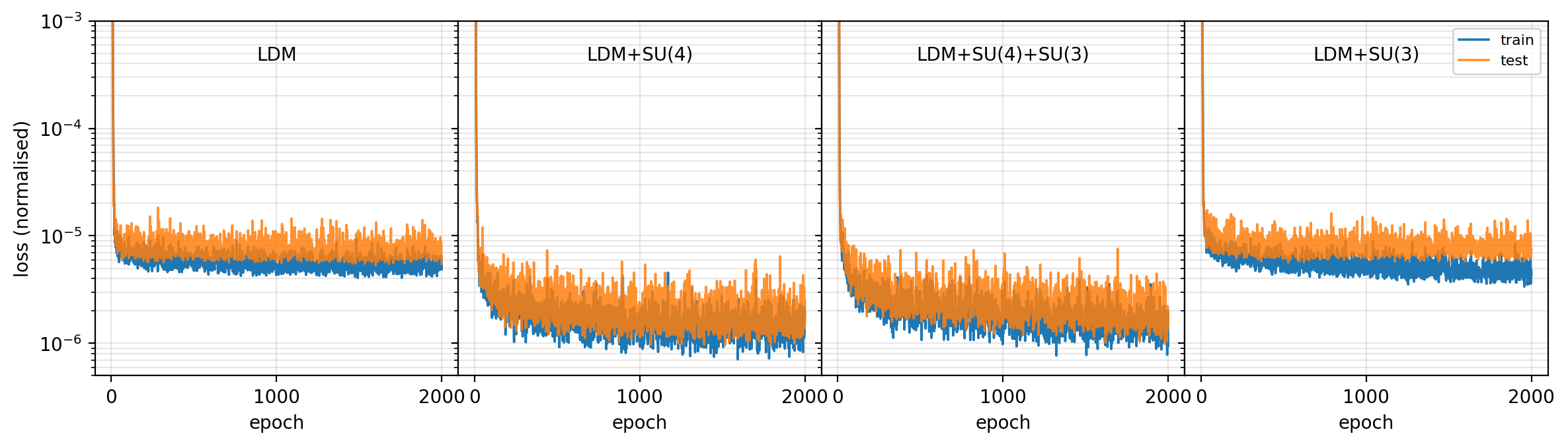
As described in Sec. 2.1 of the main text, the \(20\%\) test set is held out from training but drawn from the same distribution as the train data; it therefore serves as an overfitting monitor, distinct from the
AME2020 validation set that measures extrapolation. Figure 8 shows the per-epoch train and test losses for the FINN across all feature sets. In every case the two curves descend together and plateau at
essentially the same level, with no upturn of the test loss at late epochs. The small train-test gap confirms that the networks are not memorizing the training nuclei [51]. Consequently, the larger error on the AME2020 validation set (Table 1 of the main text) reflects genuine extrapolation to newly measured, often more exotic nuclei rather than overfitting. The flatness of
the test curve also indicates that early stopping offers no benefit here, as the GK loss already regularizes the training effectively.
9 Normalization of the data↩︎
The features used in our models span widely different scales: the bulk inputs \((Z, N, A^{2/3}, T_z)\) range over tens to hundreds, the harmonic oscillator quanta \(N_{\hbar\omega}\) grow into the hundreds, and the \(\rm SU(4)\) and \(\rm SU(3)\) Casimir eigenvalues grow even faster with nucleon number. Feeding such heterogeneous magnitudes directly into a neural network is detrimental: features with large numerical values dominate the gradients irrespective of their physical relevance, the optimization becomes ill-conditioned, and the inputs are pushed into the saturated regions of the activation functions. Hence, we standardize every input feature and the target binding energy to zero mean and unit variance through \(z\)-score normalization, \[\tilde{x}_i = \frac{x_i - \mu_i}{\sigma_i + \epsilon}, \qquad \tilde{y} = \frac{y - \mu_y}{\sigma_y + \epsilon}, \label{eq:zscore}\tag{3}\] where \(\mu_i, \sigma_i\) are the mean and standard deviation of feature \(i\), and \(\mu_y, \sigma_y\) are those of the binding energy. Here, \(\epsilon = 10^{-8}\) is a small constant that guards against division by zero for (near-)constant columns.
Crucially, the statistics \(\{\mu, \sigma\}\) are computed on the train set only and then applied to the test and validation sets. This prevents information from the held-out nuclei from leaking into the preprocessing, so that the test and validation errors remain honest measures of generalization and extrapolation. Since the target is also standardized, the network learns in normalized units; all predictions are mapped back to physical units (MeV) through the inverse transform \(y = \tilde{y}\,\sigma_y + \mu_y\) before RMSE is reported. After standardization the features are of comparable magnitude, which balances the gradients, accelerates and stabilizes convergence, and ensures that the relative importance the models assign to each feature reflects its predictive value.
10 Smooth versus disruptive activation functions↩︎
The choice of activation function is usually regarded as a minor architectural detail, but for nuclear masses it carries physical meaning. The binding energy is not a smooth function of \(N\) and \(Z\), specifically, at every magic number the nuclear surface stiffens and the binding is sharply enhanced, producing a near-discontinuity in the first derivative of \(BE\). Accordingly, the two-neutron separation energy \(S_{2n}(Z,N) = BE(Z,N) - BE(Z,N-2)\) drops abruptly upon crossing a neutron shell closure. A network built from disruptive activation functions [e.g., the rectified linear unit, ReLU\((x) = \max(0,x)\)] is a piecewise function of its inputs and can represent such kinks, whereas a network built from smooth, infinitely differentiable activations [e.g., the hyperbolic tangent, Tanh\((x)\), or the sigmoid linear unit, SiLU\((x) = x/(1+e^{-x})\)] must approximate every kink with a rounded transition.
To test the consequence of this distinction, we conduct an experiment by retraining the FINN four times, identical in every aspect—same architecture, feature set, optimizer, loss, and training schedule—differing only in the hidden activation. In particular, we compare two piecewise-linear activations—ReLU and its parametric variant PReLU [PReLU\((x) = x\) for \(x>0\) and \(\alpha x\) for \(x<0\), with a learnable slope \(\alpha\)]—against two smooth ones, Tanh and SiLU. The random seed is also fixed so the models share an identical weight initialization and mini-batch ordering.
| Activation | Train | Test | Validation |
|---|---|---|---|
| ReLU | 0.444 | 0.555 | 0.894 |
| PReLU | 0.411 | 0.552 | 0.624 |
| Tanh | 0.525 | 0.579 | 0.811 |
| SiLU | 0.611 | 0.677 | 0.826 |
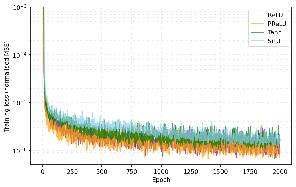
Figure 9 shows the training loss versus epoch. All four converge within a few hundreds of epochs, but the piecewise-linear networks thereafter settle to a consistently lower loss. Moreover, as shown in Table 2, the train and test RMSEs are the lowest with the ReLU and PReLU activations, and the PReLU network achieves the best extrapolation on the validation set. That the ReLU is outperformed by its parametric version can be explained by the fact that one of the FINN’s features is the isospin projection \(T_z\), which is positive (negative) for neutron(proton)-rich nuclei. The ReLU, which only returns positive output, tends to gravitate toward positive inputs and ignore negative ones, whereas the PReLU takes into account both and simultaneously generates the desired discontinuity.
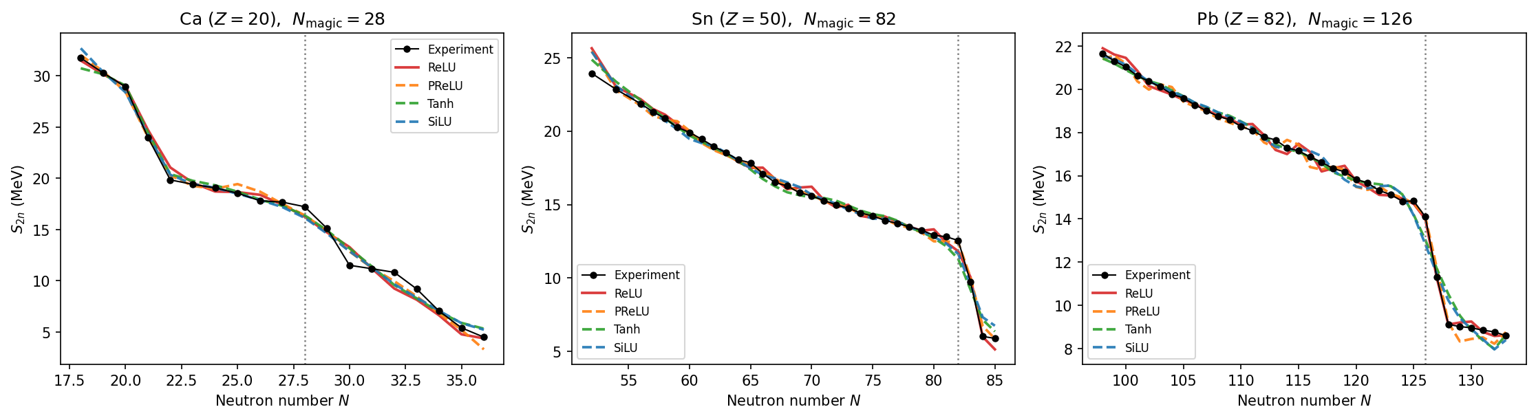
To probe deeper the advantage of each activation function at the shell closures, we compare the predicted \(S_{2n}\) along three isotopic chains that each cross a major neutron magic number, namely \(^{48}\)Ca (\(N=28\)), \(^{132}\)Sn (\(N=82\)), and \(^{208}\)Pb (\(N=126\)). The experimental \(S_{2n}\) falls sharply just past each closure, which is tracked closely by the piecewise-linear ReLU and PReLU networks as demonstrated in Fig. 10, whereas the smooth activations smear it out. Quantitatively, the shell gap \(\Delta S_{2n} = S_{2n}(N_{\rm magic}) - S_{2n}(N_{\rm magic}+2)\) is reproduced best by the piecewise-linear activations at the two heavy, well-developed closures (Table 3); specifically, the PReLU and ReLU respectively recover \(4.89\) MeV and \(4.88\) MeV at \(^{208}\)Pb against the experimental \(4.98\) MeV, and \(5.68\) MeV and \(5.82\) MeV at \(^{132}\)Sn against \(6.53\) MeV, while Tanh and SiLU capture less than two thirds of each gap.
| Chain | Exp. | ReLU | PReLU | Tanh | SiLU |
|---|---|---|---|---|---|
| \(^{48}\)Ca (\(N=28\)) | \(5.72\) | \(2.96\) | \(3.52\) | \(3.23\) | \(3.27\) |
| \(^{132}\)Sn (\(N=82\)) | \(6.53\) | \(5.82\) | \(5.68\) | \(4.13\) | \(4.30\) |
| \(^{208}\)Pb (\(N=126\)) | \(4.98\) | \(4.88\) | \(4.89\) | \(2.51\) | \(2.59\) |
11 Inclusion of the third-order \(\rm SU(4)\) Casimir operator↩︎
In this section, we provide justification for the exclusion of the cubic Casimir \(\mathcal{C}_3 [\rm SU(4)]\) from the feature set. As given in Sec. 6, the expression for \(\langle \mathcal{C}_3 \rangle\) eigenvalue carries the overall prefactor \((P - P'')\), thus \(\langle \mathcal{C}_3 [\rm SU(4)] \rangle = 0\) when \(P = P''\), i.e., whenever the leading irrep of the nucleus is self-conjugate. For the dominant lowest-\(\mathcal{C}_2\) irrep, the labels \((P, P', P'')\) are fixed by the nucleon numbers and fall into four categories:
| Category | \((P, P', P'')\) | \(\langle \mathcal{C}_3 \rangle\) |
|---|---|---|
| even-even | self-conjugate | \(0\) |
| odd-odd | self-conjugate | \(0\) |
| \(Z\) even, \(N\) odd | \((1,\, |N-Z|/2 - 1/2,\, 0)\) | \(> 0\) |
| \(Z\) odd, \(N\) even | \((0,\, |N-Z|/2 - 1/2,\, 1)\) | \(< 0\) |
Both even-mass families (even-even and odd-odd) are self-conjugate (\(P = P''\)), so every even-\(A\) nucleus has \(\langle \mathcal{C}_3 [\rm SU(4)] \rangle \equiv 0\). Only odd-\(A\) nuclei carry a nonzero value, and its sign is set entirely by which nucleon species is unpaired. The two neighbors \((N,Z)\) and \((N-1, Z+1)\) share the same odd mass number but swap these roles, which leads to the sign fluctuation noted in Sec. 2.2 of the main text and is reflected quantitatively via the low maximal information coefficients of \(\mathcal{C}_3 [\rm SU(4)]\) with respect to the bulk and \(\rm SU(3)\) features (see Fig. 2 of the main text).
This structure is borne out by the data: across the \(2457\) nuclei in our dataset, all \(1227\) even-\(A\) nuclei have \(\langle \mathcal{C}_3 [\rm SU(4)] \rangle = 0\) identically, whereas the \(1230\) odd-\(A\) nuclei are nonzero and split by sign into the \(Z\)-even/\(N\)-odd (mean \(\approx +120\)) and \(Z\)-odd/\(N\)-even (mean \(\approx -118\)) classes. This sign assignment holds exactly for \(N \geq Z\); the only exceptions (\(\sim\!4\%\) of odd-\(A\) nuclei) lie deep on the proton-rich side (\(Z > N\)), where the \((P - P'')\) prefactor reverses as protons outnumber neutrons. It is unlikely for a feature that vanishes over half the nuclear chart and alternates in sign over the remainder to encode any smooth systematic trend in the binding energy. In particular, after normalization, this produces a feature that oscillates between approximately \(-1\) and \(+1\), which can make it difficult for the neural network to extract a smooth physical trend. Moreover, when this feature is introduced in the training, the SHAP ranking of feature importance shows a negligible contribution to the learning, as if it were effectively very noisy information.
Nevertheless, the physical information encoded in the third-order SU(4) Casimir could be important for nuclear binding, as there is an overall trend of the intensity of the fluctuations, with sharper ones for heavier species and for lower \(Z\) nuclei along isotonic chains. In order to retain the information carried by this operator, we split it in two feature maps, smotting the oscillation separating the positive and negative values by defining two nonnegative derived features as follows \[\mathcal{C}_3^+[\mathrm{SU}(4)] = \max\left(\mathcal{C}_3[\mathrm{SU}(4)], 0\right),\] \[\mathcal{C}_3^-[\mathrm{SU}(4)] = \max\left(-\mathcal{C}_3[\mathrm{SU}(4)], 0\right).\] This transformation preserves the magnitude and sign information of the original feature, since \(C_3[\mathrm{SU}(4)] = \mathcal{C}_3^+[\mathrm{SU}(4)] - \mathcal{C}_3^-[\mathrm{SU}(4)]\), but represents the positive and negative branches as two separate smooth, nonnegative channels. This is more convenient for training because the model no longer has to learn a single rapidly sign-changing feature. Instead, it can assign independent weights to the positive and negative sectors, making it easier to identify whether each branch carries useful physical information for the \(BE\) prediction. Figure 11 shows the two new features obtained with this procedure.
![Figure 11: \mathcal{C}_3^+ [\rm SU(4)] and \mathcal{C}_3^- [\rm SU(4)] features derived from the cubic \rm SU(4) Casimir operator. All values are non-negative.](/article/2606.28287/C3_pos_neg_2.png "fig:")
| Activation | Train RMSE | Test RMSE | Validation RMSE |
|---|---|---|---|
| PReLU (\(\lambda = 1.0\)) | 0.479 | 0.662 | 1.145 |
| PReLU (\(\lambda = 2.0\)) | 0.714 | 0.841 | 1.311 |
| PReLU (\(\lambda = 4.0\)) | 0.485 | 0.700 | 1.039 |
| ReLU (\(\lambda = 1.0\)) | 0.493 | 0.796 | 1.218 |
| ReLU (\(\lambda = 2.0\)) | 0.466 | 0.721 | 1.218 |
| ReLU (\(\lambda = 4.0\)) | 0.400 | 0.666 | 1.535 |
We train the FINN’s full feature set [i.e., LDM+\(\rm SU(4)\)+\(\rm SU(3)\)] augmented with these two derived features, first without any modification to the network architecture (PReLU activation, \(10^{-3}\) learning rate, GK weight \(\lambda = 2.0\), no weight decay), followed by testing with an alternative activation function and different GK weights. The results are reported in Table 4. Overall, we observe a deterioration to the model’s performance as demonstrated by higher RMSEs. In particular, most errors are above the FINN’s RMSE for the full feature set reported in Table 1 of the main text, especially on the validation set (all exceeding \(1.0\) MeV), which implies that the model generalizes badly on unseen data. These results lead to our conclusion that adding the proxy non-negative features derived from the cubic \(\rm SU(4)\) Casimir does not supply more reliable predictive information to the model. Even though the information carried by this third-order operator may help capture odd-\(A\) structure distinct from that of even-\(A\) nuclei, it is probably either too localized or too discontinuous to improve a global mass model, hence, it should be ultimately excluded from the feature set of nuclear binding.
12 Pairing effect↩︎
To check whether the WINN misses pairing correlations, we examine the WINN mass residuals, \(BE_{\rm pred} - BE_{\rm exp}\), separated into three classes of even-even, odd-\(A\), and odd-odd nuclei (Fig. 12). If the pairing effect were not fully captured, one would observe a systematic underbinding for even-even nuclei, a systematic overbinding for odd-odd nuclei, and a noticeable odd-even oscillation of the residuals. We observe none of these; in fact, the class-averaged residuals are small (within \(\sim\!0.25\) MeV) and of the same negative sign, with no even-even/odd-odd inversion and no odd-even staggering. The pairing systematics are therefore already absorbed by the model through the term \(a\) in Eq. (1) of the main text, as it is trained to learn the \((N,Z)\)-dependent “leftover” of binding from the symmetry descriptors, which could include both the volume energy and pairing effect. Note that we find a degradation on the validation RMSE upon adding an explicit pairing term [\(\delta(N,Z)\)].
One may wonder how it is possible for the NN to learn the pairing contribution that is not a smooth function of \(N\) and \(Z\). We attribute our model’s ability to capture this jagging to the ReLU activation function, which is not a smooth one. In principle, one can use a large and deep NN to approximate any function—with sufficient data, the model should be able to pick up a functional representation of the output in terms of the input features. However, since there are only two and a half thousand nuclei discovered to date, the choice of the activation function helps in approximating the fine detail of the \((N,Z)\) dependence, including the breaking of smoothness of \(BE\).

References↩︎
The Pearson and Spearman coefficients are zero for these relationships, showing that they are unable to detect these complex correlations, depsite the visible trends in the scatter plots.↩︎