Disentangling Continuous-Time Latent Dynamics: Identifiability of Latent SDEs via Diffusion Shifts
June 26, 2026
Abstract
Causal representation learning for time series has developed strong identifiability results in discrete-time latent causal models, but identifiability in continuous-time latent stochastic differential equation (SDE) models remains largely open. We address this gap using environment-induced shifts in diffusion covariance. We study additive-noise latent SDEs observed through an unknown nonlinear diffeomorphism, with shared drift but environment-specific diffusion covariance. We show that two diagonal diffusion regimes with pairwise distinct coordinate-wise variance ratios identify the latent coordinates up to permutation and scaling, without any sparsity assumption on the drift. We first prove this result for linear Ornstein–Uhlenbeck systems and then extend it to general additive-noise latent SDEs. Under mild smoothness, the instantaneous drift-Jacobian causal graph is identifiable up to the same permutation. We propose a two-stage estimator for latent disentanglement and optional graph recovery; experiments on synthetic systems confirm the predicted identifiability boundary, and an application to Hardanger Bridge monitoring data illustrates the approach on real sensor trajectories.
1 Introduction↩︎
Causal representation learning (CRL) seeks to recover latent causal variables and their structural relations from entangled observations [1]. This problem is especially compelling for time series, where causal structure underlies explanation, forecasting, and decision-making in domains such as climate science, biology, healthcare, and economics [2], [3]. In many temporal settings, however, the measured variables are not the causal variables of interest: video frames, sensor streams, and multivariate readouts are often nonlinear mixtures of latent dynamical factors. Without additional structure, those factors are not identifiable from observations alone [4], [5]. Temporal CRL therefore asks how temporal dependence, environmental variation, or interventions can break nonlinear mixing ambiguities and make latent causal variables identifiable.
1.0.0.1 Motivation.
Many scientific and engineered systems evolve in continuous time, are sampled irregularly, and are intrinsically stochastic. Stochastic differential equations (SDEs) provide a standard language for such dynamics [6], [7]. Continuous-time latent and controlled dynamics are also widely used in machine learning through neural ODEs, latent ODEs, neural controlled differential equations, and neural SDEs [8]–[11]. Continuous time also exposes objects that are blurred by a discrete-time view, including drift, diffusion, quadratic variation, and instantaneous dependence. This distinction is important for representation learning: the drift describes the deterministic law of motion, whereas the diffusion describes the scale and orientation of unresolved stochastic fluctuations.
In many latent dynamical systems, it is natural for the deterministic law of motion to remain stable across environments while the stochastic forcing changes. A bridge may have the same structural dynamics while wind and traffic loads change the amplitude and direction of stochastic excitation; a cardiovascular system may retain the same regulatory feedback loops while exercise or stress changes physiological variability; and a power grid may retain the same network dynamics while stochastic load fluctuations vary across demand or weather regimes. Such regime variation is often easier to observe than direct interventions on latent causal mechanisms. Such variation also provides a form of side information specific to continuous time: diffusion leaves a local quadratic-variation signature in the observed path, even though this signature is distorted by the unknown nonlinear mixing. This leads to the central identifiability question of this paper: when can diffusion shifts alone recover the latent coordinate system of a continuous-time SDE model from nonlinear observations?
1.0.0.2 Challenges.
Existing identifiable nonlinear ICA and temporal CRL results show that side information can break nonlinear mixing ambiguities, but their identifiability theory is largely built for discrete-time settings, using finite-lag transitions, autoregressive mechanisms, or temporal context on a grid [12]–[16]. Conversely, work on continuous-time SDE identification and causal discovery typically assumes that the stochastic state itself is observed, rather than seen only through an unknown nonlinear observation map [17]–[21]. The latent continuous-time setting is harder: the state is observed only after an unknown nonlinear mixing, and the target is not merely a predictive state but the latent coordinate system and its instantaneous drift-Jacobian graph. What is missing is a theorem-level CRL account for continuous-time latent SDE state coordinates observed only through such a mixing. The central difficulty is that diffusion covariance is not invariant under nonlinear coordinate changes: in observed coordinates, local quadratic variation is the latent covariance transformed by the Jacobian of the unknown mixing. A single diffusion regime therefore cannot determine which latent axes are the causal coordinates. Our key observation is that two diagonal diffusion regimes with distinct coordinate-wise variance ratios impose simultaneous constraints on the same unknown Jacobian. These constraints reduce the remaining ambiguity to permutation and scaling, which in turn makes instantaneous drift-graph recovery well defined.
1.0.0.3 Contributions.
We study additive-noise latent SDEs observed through an unknown nonlinear diffeomorphism across two environments that share the latent drift but differ in diffusion covariance. Our contributions are: We formulate this continuous-time CRL problem and identify diffusion shifts as the source of side information: two diagonal regimes with coordinate-wise distinct variance ratios are sufficient to anchor the latent coordinate system. We prove identifiability first for linear Ornstein–Uhlenbeck systems and then for general additive-noise latent SDEs: the latent coordinate system is recovered up to permutation and scaling without any sparsity assumption on the drift, and under mild smoothness the instantaneous drift-Jacobian causal graph is identifiable up to the same permutation. We turn the theory into a practical two-stage estimator: diffusion-based disentanglement followed, when graph recovery is desired, by sparse drift regression. Synthetic experiments validate the predicted identifiability boundary, and a Hardanger Bridge monitoring study illustrates the estimator on real sensor trajectories.
2 Problem setup and target↩︎
We consider two environments, indexed by \(e\in\{1,2\}\). In environment \(e\), the latent state \(z_t^{(e)}\in\mathbb{R}^d\) evolves according to the additive-noise SDE \[\label{eq:generic95latent95sde95setup} dz_t^{(e)} = f(z_t^{(e)})\,dt + G_e\,dW_t^{(e)}, \qquad x_t^{(e)} = g(z_t^{(e)}),\tag{1}\] where \(x_t^{(e)}\in\mathbb{R}^d\) is the observed process, \(W_t^{(e)}\) is a standard \(d\)-dimensional Brownian motion, \(f:\mathbb{R}^d\to\mathbb{R}^d\) is the latent drift, \(G_e\in\mathbb{R}^{d\times d}\) is the environment-specific diffusion matrix, and \(g:\mathbb{R}^d\to\mathbb{R}^d\) is an unknown nonlinear observation map. The two environments share the same latent drift \(f\) and differ only through their diffusion covariances. In the linear Ornstein–Uhlenbeck special case studied first in Section 3.1, the drift takes the form \(f(z)=Az\) for some matrix \(A\in\mathbb{R}^{d\times d}\). Throughout, we write \(\Sigma_e := G_e G_e^\top\) for the latent diffusion covariance in environment \(e\).
The latent dynamics are autonomous: \(f\) has no explicit time dependence, so the causal mechanism is not explicitly time varying. In continuous-time causal models for SDEs, a parent relation is typically induced when one variable enters another variable’s drift or diffusion coefficient [18], [20], [22]. In our additive-noise setting, however, the diffusion matrices \(G_e\) are constant in \(z\), so no variable enters another variable’s diffusion coefficient. We therefore represent the latent causal structure by the drift alone. In the linear OU case, this reduces to the support pattern of \(A\), which is constant over time. In the general nonlinear case, we work with the instantaneous drift-Jacobian graph at state \(z\), namely the support pattern of \(Df(z)\); this graph may depend on the current state, but not explicitly on time.
Our goal is to characterize conditions under which the pair of observed path laws from the two environments is sufficient to recover the latent coordinate system up to permutation and coordinate-wise scaling, and to identify the corresponding latent causal structure up to the same permutation. The precise identifiability statements are given in Section 3.
3 Identifiability theory↩︎
3.1 Linear OU systems↩︎
We begin with the linear-drift case, where the identification mechanism can be seen most transparently. This case is a conceptual starting point rather than a restrictive assumption. In the OU setting, the diffusion comparison already contains the core disentanglement mechanism, and the state-space coverage step is automatic from the Gaussian transition law. This lets us isolate the role of the two regimes with minimal additional technical overhead.
3.1.0.1 Assumptions.
We state the shared assumptions for two observationally equivalent latent representations: the reference parametrization and an alternative tilded parametrization. Both the OU theorem below and the general nonlinear theorem in Section 3.2 rely on these four assumptions.
Shared two-regime assumptions
(Regularity) \(g,\tilde{g}:\mathbb{R}^d\to\mathbb{R}^d\) are \(C^2\) diffeomorphisms, and \(\varphi := \tilde{g}^{-1}\circ g\).
(Trajectory-law equivalence in each regime) For each \(e\in\{1,2\}\), \[\{x_t^{(e)}\}_{t\in[0,T]} \overset{d}{=} \{\tilde{x}_t^{(e)}\}_{t\in[0,T]} \quad \text{in } C([0,T];\mathbb{R}^d).\]
(Diagonal positive-definite covariances) For each \(e\in\{1,2\}\), the diffusion covariances \[\Sigma_e := G_e G_e^\top, \qquad \tilde{\Sigma}_e := \tilde{G}_e \tilde{G}_e^\top\] are diagonal and positive definite.
(Two-regime separation; simple spectrum) The diagonal entries of \(\Sigma_1^{-1}\Sigma_2\) are pairwise distinct; equivalently, if \(\Sigma_e=\operatorname{diag}(\sigma_{e,1}^2,\dots,\sigma_{e,d}^2)\), then \[\frac{\sigma_{2,i}^2}{\sigma_{1,i}^2} \neq \frac{\sigma_{2,j}^2}{\sigma_{1,j}^2} \qquad \forall i\neq j.\]
Assumptions (S1) and (S2) are standard in identifiable nonlinear ICA and causal representation learning: one posits an invertible nonlinear mixing and asks whether two latent parametrizations inducing the same observed law must be equivalent, as in [12]–[15], [23], [24]. Assumption (S3) is a nondegeneracy condition on the additive noise. It fixes coordinatewise diffusion geometry and rules out singular directions. Related diagonal or block-diagonal noise restrictions are also common in continuous-time structure learning and path-space causal discovery [18], [20], [22].
Assumption (S4) is the separating condition: each latent coordinate carries a distinct diffusion-ratio fingerprint across environments. This is generically mild: failure occurs only when two ratios coincide exactly, a lower-dimensional subset of the diagonal covariance parameter space. It is also the continuous-time analogue of the variability conditions that drive identifiability in temporal and multi-environment CRL [15], [23], [25]–[27]. In the OU case, no additional support assumption is needed, because every nondegenerate Gaussian transition has full support on \(\mathbb{R}^d\).
Throughout this section, \(\varphi = \tilde{g}^{-1}\circ g\) denotes the change of coordinates between two observationally equivalent latent parametrizations: \(\tilde{z}=\varphi(z)\) describes the same underlying state in the alternative coordinate system. We write \(D\varphi(z)\) for its Jacobian. The main identifiability question is whether \(\varphi\) must reduce to a monomial affine transformation.
Theorem 1 (OU identifiability from two diagonal diffusion regimes). For each \(e\in\{1,2\}\), consider reference and tilded latent OU parametrizations: \[\begin{align} d z_t^{(e)} &= A\,z_t^{(e)}\,dt + G_e\,dW_t^{(e)}, & x_t^{(e)} &= g(z_t^{(e)}), \tag{2}\\ d \tilde{z}_t^{(e)} &= \tilde{A}\,\tilde{z}_t^{(e)}\,dt + \tilde{G}_e\,d\tilde{W}_t^{(e)}, & \tilde{x}_t^{(e)} &= \tilde{g}(\tilde{z}_t^{(e)}). \tag{3} \end{align}\] Assume (S1)–(S4). Then there exist a constant monomial matrix \(L=\Pi\Lambda\) and a constant vector \(c\in\mathbb{R}^d\) such that \[\begin{gather} D\varphi(z)\equiv L,\qquad \varphi(z)=Lz+c \quad (z\in\mathbb{R}^d),\\ \tilde{\Sigma}_e = L\Sigma_eL^\top,\qquad \tilde{A} L = L A,\qquad \tilde{A} c = 0 \quad (e\in\{1,2\}). \end{gather}\] Equivalently, \(\tilde{A} = LAL^{-1}\). Hence the observed path laws identify the latent coordinate system up to permutation and scaling, together with a possible constant shift if \(\varphi(0)\neq 0\). For \(E_A:=\{(j\to i):A_{ij}\neq 0\}\), \(E_{\tilde{A}}:=\{(j\to i):\tilde{A}_{ij}\neq 0\}\), and \(\Pi e_j=e_{\pi(j)}\), \[(j\to i)\in E_A \quad \Longleftrightarrow \quad (\pi(j)\to \pi(i))\in E_{\tilde{A}}.\] Thus the latent causal structure in the OU case is identifiable up to the same permutation.
3.1.0.2 Proof sketch.
The full proof is deferred to Appendix 10. Equality of observed path laws allows a coupling with \(\tilde{z}_t^{(e)}=\varphi(z_t^{(e)})\) almost surely in each regime. Itô’s formula and quadratic variation give \(D\varphi(z_t^{(e)})\Sigma_e D\varphi(z_t^{(e)})^\top=\tilde{\Sigma}_e\) along trajectories. For OU dynamics, the latent state at any positive time has a strictly positive Gaussian density on \(\mathbb{R}^d\), so this identity extends to every state \(z\in\mathbb{R}^d\). Whitening with respect to the first regime reduces the problem to an orthogonal matrix field. The second regime and the simple-spectrum condition in (S4) force that field to be a signed permutation at every \(z\). Continuity then makes the signed permutation constant, so \(D\varphi\) is a constant monomial matrix and \(\varphi\) is affine; substituting into the drift relation gives \(\tilde{A} L=LA\), yielding the coordinate-system and graph statements.
3.2 General latent SDEs↩︎
We now turn to nonlinear drifts. As in the OU case, \(\varphi := \tilde{g}^{-1}\circ g\) denotes the coordinate change between two observationally equivalent latent parametrizations, with Jacobian \(D\varphi(z)\). The diffusion comparison still provides the core algebraic step. Only the support argument changes: an identity first obtained along sample paths must be extended to \(\mathbb{R}^d\) without explicit Gaussian transition densities.
The shared assumptions (S1)–(S4) remain in force, and (S5) ensures well-defined continuous semimartingales and the open-set positivity step. This is a standard additive-noise SDE regularity condition: it requires continuous drifts and weak well-posedness with continuous sample paths, but not strong solutions or closed-form transition densities. Appendix 10.5 gives further discussion.
Theorem 2 (Latent SDE identifiability from two diffusion regimes). For each \(e\in\{1,2\}\), consider reference and tilded latent SDE parametrizations: \[\begin{align} d z_t^{(e)} &= f(z_t^{(e)})\,dt + G_e\,dW_t^{(e)}, & x_t^{(e)} &= g(z_t^{(e)}), \tag{4}\\ d \tilde{z}_t^{(e)} &= \tilde{f}(\tilde{z}_t^{(e)})\,dt + \tilde{G}_e\,d\tilde{W}_t^{(e)}, & \tilde{x}_t^{(e)} &= \tilde{g}(\tilde{z}_t^{(e)}). \tag{5} \end{align}\] Assume the shared two-regime conditions (S1)–(S4), and in addition:
Additional regularity assumption for nonlinear SDEs
Then there exist a constant monomial matrix \(L=\Pi\Lambda\) and a constant vector \(c\in\mathbb{R}^d\) such that \[\begin{gather} D\varphi(z)\equiv L,\qquad \varphi(z)=Lz+c \quad (z\in\mathbb{R}^d),\\ \tilde{\Sigma}_e = L\Sigma_eL^\top \quad (e\in\{1,2\}),\qquad \tilde{f}(Lz+c)=L f(z) \quad (z\in\mathbb{R}^d). \end{gather}\] Consequently, the observed path laws identify the latent coordinate system up to permutation and scaling, together with a possible constant shift \(c\).
Remark 3 (Support coverage is automatic). The proof only needs that, for some \(t_\star>0\), the law of \(z_{t_\star}^{(e)}\) has full support on \(\mathbb{R}^d\). Under (S3) and (S5), this follows from the open-set positivity lemma in Appendix 10.3, which covers arbitrary initial laws.
3.2.0.1 Proof sketch.
The proof, deferred to Appendix 10, reuses the OU argument. The coupling, quadratic-variation comparison, and whitening/simple-spectrum steps are unchanged. The new ingredient is the open-set positivity lemma, which upgrades the along-trajectory covariance identity to a pointwise identity on \(\mathbb{R}^d\) without Gaussian transition densities. The rest follows as in the OU case: \(D\varphi\) is a constant monomial matrix, hence \(\varphi(z)=Lz+c\), and the same semimartingale comparison gives \(\tilde{f}(Lz+c)=Lf(z)\).
Under (S1)–(S5), Theorem 2 shows that any observationally equivalent latent coordinate change must be a monomial affine map. When \(f\) and \(\tilde{f}\) are \(C^1\), differentiating \(\tilde{f}(Lz+c)=Lf(z)\) yields the drift-Jacobian graph statement.
Corollary 1 (Drift-Jacobian graph identifiability up to permutation). Under the assumptions of Theorem 2, assume additionally that \(f,\tilde{f}\) are \(C^1\). Let \(J_f(z):=Df(z)\), \(E_f(z):=\{(j\to i):(J_f(z))_{ij}\neq 0\}\), and define \(J_{\tilde{f}},E_{\tilde{f}}\) analogously. Then \[D\tilde{f}(Lz+c)=L\,Df(z)\,L^{-1} \qquad \forall z\in\mathbb{R}^d,\] so the instantaneous drift-Jacobian causal graphs are identified up to the permutation induced by \(\Pi\). Writing \(\Pi e_j=e_{\pi(j)}\), equivalently, \[(j\to i)\in E_f(z) \quad \Longleftrightarrow \quad (\pi(j)\to \pi(i))\in E_{\tilde{f}}(Lz+c).\]
4 Two-stage estimation↩︎
We translate the identifiability results into a two-stage estimator. Stage 1 learns the latent coordinate system from short-time transition statistics across the two regimes. Stage 2 is optional and estimates a sparse drift graph when explicit graph recovery is desired.
4.1 Model parameterization↩︎
We observe trajectories \(\{x_{t_0}^{(e)},x_{t_1}^{(e)},\dots,x_{t_N}^{(e)}\}\) from two regimes \(e\in\{1,2\}\) at uniform intervals \(\Delta t\). The encoder \(h_\theta\) maps observations into a learned latent coordinate system, playing the estimator-side role of \(\tilde{g}^{-1}\) in Sections 3.1–3.2. We keep the tilde notation \((\tilde{z},\tilde{f},\tilde{\Sigma}_e)\) for learned coordinates, drift, and diffusion parameters, with \(\theta,\psi\) denoting parametric components. Our learnable model consists of three components:
an encoder \(h_\theta:\mathbb{R}^d\to\mathbb{R}^d\), implemented as an MLP in our experiments, with \(\tilde{z}_t=h_\theta(x_t)\);
a differentiable drift model \(\tilde{f}_\psi:\mathbb{R}^d\to\mathbb{R}^d\), shared across regimes and implemented as either a linear map or an MLP;
diagonal per-regime diffusion parameters \(\tilde{\Sigma}_e=\operatorname{diag}(\tilde{\sigma}_{e,1}^2,\ldots,\tilde{\sigma}_{e,d}^2)\), parameterized by \(\log \tilde{\sigma}_{e,i}^2\) to ensure positivity.
We do not enforce \(h_\theta\) to be globally invertible during training, so the Stage 1 likelihood below is interpreted as a pseudo-likelihood in general.
4.2 Stage 1: short-time transition fitting↩︎
Stage 1 uses the short-time behavior of additive-noise SDEs. For small \(\Delta t\), the Euler–Maruyama discretization gives a Gaussian approximation to one-step transitions [6], [7]. In regime \(e\), the encoded-space working model is \[\label{eq:EM95transition} \tilde{z}_{t+\Delta t}\mid \tilde{z}_t,e \sim \mathcal{N}\!\Big(\tilde{z}_t + \tilde{f}_\psi(\tilde{z}_t)\,\Delta t, \tilde{\Sigma}_e\,\Delta t\Big).\tag{6}\] Equivalently, \[\tilde{z}_{t+\Delta t} = \tilde{z}_t + \tilde{f}_\psi(\tilde{z}_t)\,\Delta t + \varepsilon_t^{(e)}, \qquad \varepsilon_t^{(e)}\sim \mathcal{N}(0,\tilde{\Sigma}_e\,\Delta t).\] The diagonal \(\tilde{\Sigma}_e\) makes the one-step residual coordinates conditionally independent under this model.
If the encoded states \(\tilde{z}_t\) were observed, the per-transition negative log-likelihood, up to the additive constant \(\tfrac{d}{2}\log(2\pi\Delta t)\), is \[\label{eq:nll95ztilde} \ell_e(\tilde{z}_t,\tilde{z}_{t+\Delta t}) = \frac{1}{2}\sum_{i=1}^d \log \tilde{\sigma}_{e,i}^2 + \frac{1}{2}\sum_{i=1}^d \frac{\big(\tilde{z}_{t+\Delta t,i}-\tilde{z}_{t,i}-\tilde{f}_{\psi,i}(\tilde{z}_t)\,\Delta t\big)^2}{\tilde{\sigma}_{e,i}^2\,\Delta t}.\tag{7}\] This is the Gaussian transition score for 6 .
4.2.0.1 Observation-space objective.
We observe only \(x_t\) and set \(\tilde{z}_t=h_\theta(x_t)\). If \(h_\theta\) is a \(C^1\) diffeomorphism, the change-of-variables formula gives \[p_\theta(x_{t+\Delta t}\mid x_t,e) = p_{\tilde{z},e}\big(h_\theta(x_{t+\Delta t})\mid h_\theta(x_t)\big) \,\big|\det Dh_\theta(x_{t+\Delta t})\big|,\] where \(p_{\tilde{z},e}\) is the Gaussian density in 6 and \(Dh_\theta\) is the encoder Jacobian. The observed-data per-transition negative log-likelihood, up to the same additive constant, is \[\label{eq:nll95obs} s_e(x_t,x_{t+\Delta t}) = \ell_e\big(h_\theta(x_t),h_\theta(x_{t+\Delta t})\big) - \log\big|\det Dh_\theta(x_{t+\Delta t})\big|.\tag{8}\]
In implementation, \(h_\theta\) is differentiable but need not be globally invertible, so 8 is generally a transition pseudo-likelihood. The first term fits encoded increments to the diagonal Gaussian transition model, while the log-determinant term provides a local volume correction. If \(h_\theta\) is a \(C^1\) diffeomorphism, the same score is the exact Euler–Maruyama one-step negative log-likelihood.
4.2.0.2 Stage 1 objective.
We average the per-transition score over regimes and sampled consecutive pairs: \[\label{eq:stage195loss} \mathcal{L}_{\mathrm{S1}}(\theta,\psi,\{\tilde{\sigma}_{e,i}^2\}) = \frac{1}{2}\sum_{e=1}^{2} \mathbb{E}_{(x_t,x_{t+\Delta t})\sim\mathcal{D}_e} \Big[ s_e(x_t,x_{t+\Delta t}) \Big],\tag{9}\] where \(\mathcal{D}_e\) is the empirical distribution of consecutive pairs in regime \(e\). Stage 1 jointly learns \((\theta,\psi,\{\tilde{\sigma}_{e,i}^2\})\).
4.2.0.3 Why this objective matches the theory.
Over a short interval \(\Delta t\), the drift contributes a mean shift of order \(O(\Delta t)\), whereas the stochastic increment has standard deviation \(O(\sqrt{\Delta t})\) and covariance \(\tilde{\Sigma}_e\,\Delta t\). Diffusion therefore dominates the short-time second-order behavior. Our theory shows that this regime-dependent diagonal diffusion structure anchors the latent coordinate system. Thus 7 –9 trains the encoder to find coordinates in which short-time residual increments \[\tilde{z}_{t+\Delta t}-\tilde{z}_t-\tilde{f}_\psi(\tilde{z}_t)\,\Delta t\] fit a shared-drift, regime-specific diagonal Gaussian model. This is the finite-step analogue of the two-regime identifiability mechanism in Section 3.
4.3 Stage 2: sparse drift regression↩︎
Stage 2 is optional and used only to estimate a sparse causal graph. For latent disentanglement alone, Stage 1 is the relevant part of the pipeline.
4.3.0.1 Velocity targets.
With the encoder \(h_\theta\) frozen, we form velocity targets from encoded transitions: \[\label{eq:velocity95target} \hat{v}_t = \frac{h_\theta(x_{t+\Delta t'})-h_\theta(x_t)}{\Delta t'},\tag{10}\] where \(\Delta t'=s\Delta t\) for an integer stride \(s\ge 1\). Larger strides reduce target variance, \(\operatorname{Var}(\hat{v}_{t,i})\approx \tilde{\sigma}_{e,i}^2/\Delta t'\), at the cost of \(O(\Delta t')\) bias from time-averaging the drift.
4.3.0.2 Sparse drift estimation.
We reinitialize \(\tilde{f}_\psi\) and fit it to the velocity targets with a Jacobian sparsity penalty: \[\label{eq:stage295loss} \mathcal{L}_{\mathrm{S2}}(\psi) = \underbrace{ \frac{1}{2}\sum_{e=1}^{2} \mathbb{E}_{(\tilde{z}_t,\hat{v}_t)\sim\mathcal{D}_e} \Big\|\tilde{f}_\psi(\tilde{z}_t)-\hat{v}_t\Big\|^2 }_{\text{velocity MSE}} + \lambda_{\mathrm{sparse}} \underbrace{ \mathbb{E}_{\tilde{z}\sim\mathcal{D}_1\cup\mathcal{D}_2} \sum_{i=1}^d\sum_{j=1}^d \bigg|\frac{\partial \tilde{f}_{\psi,i}}{\partial \tilde{z}_j}(\tilde{z})\bigg| }_{\ell_1\text{ drift-Jacobian penalty}}.\tag{11}\] This stage is estimator-side only and is used when a stable sparse graph estimate is needed.
4.3.0.3 Graph extraction.
By Corollary 1, the learned drift-Jacobian zero pattern is meaningful only up to the latent permutation induced by \(\Pi\). In practice, the binary adjacency matrix is obtained by thresholding the mean absolute Jacobian at a fixed threshold \(\tau>0\): \[\overline{|D\tilde{f}_\psi|} := \mathbb{E}_{\tilde{z}\sim\mathcal{D}_1\cup\mathcal{D}_2} \big[|D\tilde{f}_\psi(\tilde{z})|\big].\]
4.3.0.4 Summary.
Algorithm 3 in Appendix 11 summarizes the training and graph-extraction procedure.
5 Experiments↩︎
5.1 Synthetic experiments↩︎
We test whether the estimator matches the identifiability boundary predicted by the theory. We use three latent drift families: dense linear OU, sparse linear OU, and nonlinear sparse drift. For each family, we compare three diffusion-regime conditions: Distinct ratios, where two environments have coordinate-wise distinct diffusion-variance ratios and hence satisfy the separation requirement in Assumption (S4); One regime, which removes environment variation; and Proportional diffusions, which keeps two environments but makes all variance ratios equal. The theory predicts coordinate recovery only under Distinct ratios.
Each drift family is tested at \(d\in\{5,7\}\) under two nonlinear mixing functions. The main-text setting uses a three-layer MLP with leaky-\(\tanh\) activation \(\phi(z)=\tanh(z)+0.1z\), yielding a \(C^\infty\) diffeomorphism that satisfies the theory’s smoothness assumptions. We also test LeakyReLU mixing as a robustness check beyond the \(C^2\) setting. To keep the main text focused, we report the \(d=5\) leaky-\(\tanh\) results below; LeakyReLU and \(d=7\) results are in Appendix 13, with the data-generating process, training pipeline, hyperparameters, and metric definitions in Appendix 12 (Table 4). We report mean correlation coefficient (MCC) for one-to-one absolute-correlation alignment between learned and true coordinates; monomial score (Mon.) for how close the mean absolute Jacobian of \(h\circ g\) is to a permutation-scaling matrix; and, for sparse linear and nonlinear drifts, graph match rate (GMR) for entrywise agreement between the thresholded learned drift-Jacobian graph and the ground-truth graph. Higher is better for all metrics.
Table 1 summarizes the quantitative results. Across all three drift families, Distinct ratios gives near-perfect MCC and high monomial scores, whereas both controls show substantially lower coordinate recovery and less monomial encoder Jacobians. In the sparse linear and nonlinear families, Distinct ratios also recovers the drift graph almost exactly. GMR is omitted for the dense linear family because sparse graph recovery is not the target there. The same qualitative pattern holds at \(d=7\) and under LeakyReLU mixing (Appendix 13).
6pt
| Drift family | Regime condition | MCC \(\uparrow\) | Mon.\(\uparrow\) | GMR \(\uparrow\) |
|---|---|---|---|---|
| Dense linear | Distinct ratios | \(\mathbf{0.9976 \pm 0.0001}\) | \(\mathbf{0.8697 \pm 0.0027}\) | – |
| Dense linear | One regime | \(0.7819 \pm 0.0160\) | \(0.4750 \pm 0.0253\) | – |
| Dense linear | Proportional diffusions | \(0.8087 \pm 0.0428\) | \(0.4940 \pm 0.0344\) | – |
| Sparse linear | Distinct ratios | \(\mathbf{0.9976 \pm 0.0002}\) | \(\mathbf{0.8920 \pm 0.0038}\) | \(\mathbf{1.0000 \pm 0.0000}\) |
| Sparse linear | One regime | \(0.7206 \pm 0.0382\) | \(0.4131 \pm 0.0349\) | \(0.5760 \pm 0.0784\) |
| Sparse linear | Proportional diffusions | \(0.7018 \pm 0.0367\) | \(0.4061 \pm 0.0269\) | \(0.6400 \pm 0.0566\) |
| Nonlinear | Distinct ratios | \(\mathbf{0.9977 \pm 0.0001}\) | \(\mathbf{0.8924 \pm 0.0035}\) | \(\mathbf{1.0000 \pm 0.0000}\) |
| Nonlinear | One regime | \(0.7331 \pm 0.0232\) | \(0.4234 \pm 0.0280\) | \(0.6800 \pm 0.0506\) |
| Nonlinear | Proportional diffusions | \(0.7531 \pm 0.0141\) | \(0.4386 \pm 0.0248\) | \(0.7840 \pm 0.0742\) |
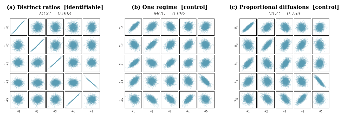
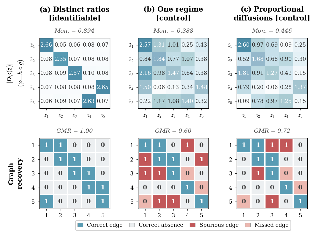
Figures 1 and 2 give qualitative diagnostics for the nonlinear \(d=5\) setting, covering both latent disentanglement and graph recovery. Each column shows one regime condition, using the same randomly selected training seed across conditions. Figure 1 shows that Distinct ratios gives a near-permutation alignment between true and learned coordinates, while the controls do not. Figure 2 shows that the corresponding \(\overline{|D\varphi|}\) matrix is near-monomial and the drift graph is recovered exactly under Distinct ratios; the controls produce denser encoder Jacobians and spurious or missed graph edges. Analogous figures for other drift families, dimensions, and mixing functions are in Appendix 13.
5.2 Real-world case study↩︎
We further test the method on operational accelerometer recordings from the Hardanger Bridge, a long-span suspension bridge instrumented for long-term wind and vibration monitoring [28], [29]. The model is trained only on bridge-deck acceleration channels; wind measurements define regimes but are not used as model inputs. This also probes robustness beyond the square diffeomorphic setting of Assumption (S1): the input has \(16\) sensor channels and the learned latent space has dimension \(d=5\). To obtain a real-world analogue of the diffusion-separation condition in Assumption (S4), we split segments within a matched wind-speed bin by turbulence intensity (TI). This keeps mean wind speed fixed while changing stochastic excitation, so low- and high-TI segments are intended to share structural dynamics while carrying different diffusion fingerprints.
We compare three regime constructions: TI-split regimes (ours), using the low- and high-TI groups as two regimes; One regime, merging the two TI groups and removing regime-specific diffusion variation; and Shuffled TI labels, preserving the two-regime training format but destroying the turbulence-based contrast. Since ground-truth latent coordinates and graphs are unavailable, we evaluate cross-seed reproducibility rather than accuracy, using pairwise mean matched absolute correlation coefficient (MCC) and graph match rate (GMR). Table 2 reports results over \(K=10\) seeds at \(d=5\). The TI-split construction gives the highest MCC and GMR, consistent with the synthetic gap between identifiable diffusion shifts and controls. Appendix 14 gives the dataset construction, training protocol, aggregate diagnostics, Assumption (S4)-style diffusion-fingerprint checks, a representative drift-Jacobian interpretation, and limitations of the real-world diagnostic.
| Condition | MCC \(\uparrow\) | GMR \(\uparrow\) |
|---|---|---|
| TI-split regimes (ours) | \(\mathbf{0.806}\) | \(\mathbf{0.877}\) |
| One regime (control) | \(0.660\) | \(0.813\) |
| Shuffled TI labels (control) | \(0.601\) | \(0.830\) |
6 Related work↩︎
Identifiable nonlinear ICA and temporal CRL show that auxiliary structure, such as nonstationarity, temporal dependence, interventions, grouping, or environment variation, can break nonlinear mixing ambiguities [12]–[16], [30], [31]. Their theorem-level temporal results, however, are largely discrete-time, based on finite-lag transitions, autoregressive mechanisms, or temporal context on a grid. Continuous-time SDE identification and causal discovery usually assume that the stochastic state is directly observed [17]–[21]; the closest latent continuous-time work treats stochastic point processes or system-level parameters rather than latent SDE state coordinates [32]–[34]. We address this gap by identifying the latent coordinate system and drift-Jacobian graph of continuous-time SDE states observed through an unknown nonlinear map, using two environments with shared drift and different diffusion covariances. Appendix 9 gives a fuller comparison.
7 Discussion and limitations↩︎
This paper gives a theorem-level account of identifiable CRL for continuous-time latent SDEs. The main message is that multi-regime diffusion structure can anchor the latent coordinate system: with shared drift and diagonal diffusion covariances whose coordinate-wise variance ratios are distinct, nonlinear observations identify the coordinates up to permutation and scaling, and the instantaneous drift-Jacobian graph follows up to the same permutation, without drift sparsity. This is a step toward CRL for continuous latent dynamics, where most temporal identifiability results are discrete-time and most continuous-time SDE identification assumes observed states. The assumptions are intentionally simple: an invertible observation map, additive state-independent diffusion, a shared drift, and separated diffusion regimes. The diffeomorphism assumption is the strongest idealization, excluding non-invertible or nonsmooth observation maps. Our LeakyReLU experiments and Hardanger study probe robustness beyond the smooth square diffeomorphic setting. Extending the theory to weaker observation maps, state-dependent noise, and imperfect regime labels remains important future work.
8 Notation↩︎
Table 3 summarizes the principal notation used throughout the paper.
6pt
| Symbol | Description |
|---|---|
| Spaces and indices | |
| \(d\) | Dimension of the latent (and observed) state space |
| \(e \in \{1,2\}\) | Environment (regime) index |
| \(t \in[0, T]\) | Continuous time; \(T\) is the time horizon |
| \(\Delta t\) | Discretization step size |
| Processes | |
| \(z_t^{(e)} \in \mathbb{R}^d\) | Latent state in environment \(e\) at time \(t\) |
| \(x_t^{(e)} \in \mathbb{R}^d\) | Observed state: \(x_t^{(e)} = g(z_t^{(e)})\) |
| \(\tilde{z}_t^{(e)} \in \mathbb{R}^d\) | Alternative latent state under the tilded parametrization |
| \(W_t^{(e)}\) | Standard \(d\)-dimensional Brownian motion |
| SDE components | |
| \(f \colon \mathbb{R}^d \to \mathbb{R}^d\) | Latent drift function (shared across environments) |
| \(A \in \mathbb{R}^{d \times d}\) | Drift matrix in the linear (OU) case: \(f(z) = Az\) |
| \(G_e \in \mathbb{R}^{d \times d}\) | Diffusion matrix in environment \(e\) |
| \(\Sigma_e = G_e G_e^\top\) | Diffusion covariance in environment \(e\) |
| \(\sigma_{e,i}^2\) | Diagonal entry of \(\Sigma_e\) (variance of coordinate \(i\) in environment \(e\)) |
| Mixing and coordinate change | |
| \(g \colon \mathbb{R}^d \to \mathbb{R}^d\) | Unknown nonlinear observation map (mixing diffeomorphism) |
| \(\varphi = \tilde{g}^{-1} \circ g\) | Latent coordinate change between two parametrizations |
| \(L = \Pi\Lambda\) | Monomial matrix (permutation and coordinate-wise scaling) |
| \(\Pi\) | Permutation matrix |
| \(\Lambda\) | Diagonal scaling matrix |
| \(c \in \mathbb{R}^d\) | Constant shift: \(\varphi(z) = Lz + c\) |
| Jacobians and causal graph | |
| \(Dg(z)\) | Jacobian of \(g\) at \(z\) |
| \(D\varphi(z)\) | Jacobian of the coordinate change \(\varphi\) at \(z\) |
| \(Df(z)\) | Jacobian of the latent drift \(f\) at \(z\) |
| \(E_f(z)\) | Instantaneous drift-Jacobian graph: \(\{(j \to i) : (Df(z))_{ij} \neq 0\}\) |
| \(\hat{E}_f\) | Estimated drift-Jacobian graph (from Stage 2) |
| \(\overline{|D\tilde{f}_\psi|}\) | Mean absolute Jacobian of the learned drift |
| Estimation | |
| \(h_\theta \colon \mathbb{R}^d \to \mathbb{R}^d\) | Encoder mapping observations to learned coordinates |
| \(\tilde{f}_\psi \colon \mathbb{R}^d \to \mathbb{R}^d\) | Learned drift model |
| \(\tilde{\sigma}_{e,i}^2\) | Learned diffusion variance for coordinate \(i\) in environment \(e\) |
| \(\hat{v}_t\) | Velocity target: \((h_\theta(x_{t+\Delta t'}) - h_\theta(x_t))/\Delta t'\) |
| \(\mathcal{L}_{\mathrm{S1}}\) | Stage 1 objective (transition negative log-likelihood) |
| \(\mathcal{L}_{\mathrm{S2}}\) | Stage 2 objective (velocity MSE \(+\) Jacobian \(L_1\) penalty) |
| \(\lambda_{\mathrm{sparse}}\) | Sparsity penalty weight (Stage 2) |
| \(\tau\) | Threshold for graph extraction from \(\overline{|D\tilde{f}_\psi|}\) |
| Evaluation metrics | |
| MCC | Mean correlation coefficient for learned/true coordinate alignment |
| Mon. | Monomial score for the mean absolute encoder Jacobian |
| GMR | Graph match rate for thresholded drift-Jacobian graphs |
9 Extended related work↩︎
9.0.0.1 Identifiable nonlinear ICA.
General nonlinear mixing is not identifiable without extra structure [4], [5]. Identifiable nonlinear ICA overcomes this via nonstationarity, temporal dependence, or auxiliary variables [12], [13], [35], [36], with structured extensions to hidden Markov and structured dependent sources [37], [38]. This line provides the main conceptual backdrop for CRL: the nonlinear mixing ambiguity can be broken once suitable side information is available.
9.0.0.2 Temporal CRL in discrete time.
A closely related CRL line studies nonlinear mixtures of latent temporal processes in discrete time. LEAP identifies latent temporal causal processes under nonstationary noise [14]; TDRL studies nonparametric time-delayed causal processes [15]; NCTRL addresses unknown nonstationarity [25]; and CtrlNS uses sparse-transition structure to recover nonstationary latent dynamics without known domain variables [16]. A parallel branch uses stronger side information: CITRIS and iCITRIS leverage interventions [30], [39], G-CaRL uses grouping information [40], and CaRiNG allows non-invertible temporal generation processes by using temporal context to recover lost information [31]. More recent extensions study instantaneous dependence via sparse latent dynamics [23], hierarchical temporal latents [41], and continuously evolving mechanisms rather than discrete switches [42]. These papers are close in spirit because they identify latent causal processes from sequential observations, but their identifying arguments are built around discrete observations, transition factorizations, or auxiliary mechanism structure rather than continuous-time SDE diffusion structure. Our object of interest is a continuous-time latent SDE path, and our proof leverages diffusion covariance changes rather than lagged transition sparsity or intervention metadata.
9.0.0.3 Multi-environment identification and partial observability in CRL.
Beyond temporal structure, environment heterogeneity and observation structure have emerged as important sources of identifiability in CRL. Multi-environment results address unknown interventions [26], cross-domain invariance conditions [43], general environment families [27], [44], [45], and the limits of purely observational identification [46]. Multi-view and partial observability settings offer a complementary route by exploiting additional observation structure [24], [47]. Recent work has also sought unifying perspectives connecting invariance-based CRL formulations with exchangeability and causal discovery [48], [49]. Our work shares the multi-environment motivation, but the identifying structure is specifically continuous-time: the drift is invariant across environments while the diffusion covariance changes, and pairwise distinct diffusion-variance ratios pin down the latent coordinates up to permutation and scaling.
9.0.0.4 Continuous-time identification and causal discovery for stochastic processes.
A separate literature studies what can be identified when the stochastic system itself is observed. Wang et al. analyze generator identifiability for linear SDEs [17]. SCOTCH studies observed-space structure learning with neural SDEs under irregular sampling [18]. Guan et al. identify linear drift, diffusion, and causal structure from temporal marginals [19]. Manten et al. derive path-space conditional independence constraints and corresponding tests for SDE models [20], and extend the graphical treatment to asymmetric independence on path spaces [22]. Zweig et al. analyze identifiability of interventional SDEs from stationary distributions [21]. Among continuous-time latent-process CRL papers, Ren et al. [32] study identifiable CRL for continuous-time latent stochastic point processes, not latent SDE state coordinates. Closely related dynamical-systems papers connect CRL with trajectory-specific or system-parameter identification [33], [34]. Our paper differs from all of these in the recovery target: we identify continuously evolving latent state coordinates and their instantaneous Jacobian graph from unknown nonlinear mixtures, using two environments with shared drift and changed diffusion.
10 Deferred technical material↩︎
10.1 Auxiliary lemmas↩︎
Lemma 1 (Orthogonal conjugation of a diagonal matrix with simple spectrum). Let \(K=\mathrm{diag}(k_1,\dots,k_d)\in\mathbb{R}^{d\times d}\) have real pairwise distinct diagonal entries, \(k_i\neq k_j\) for all \(i\neq j\). Let \(Q\in \mathbb{R}^{d\times d}\) be an orthogonal matrix. If \(QKQ^\top\) is diagonal, then \(Q\) is a signed permutation matrix: there exists a permutation \(\pi\) and signs \(s_i\in\{\pm 1\}\) such that \[Q e_i = s_i e_{\pi(i)}\quad\text{for all }i,\] equivalently \(Q = \Pi S\) where \(\Pi\) is a permutation matrix and \(S\) is diagonal with \(\pm 1\) entries. In particular, \(QKQ^\top = \Pi K \Pi^\top\).
Proof. Because \(K\) is diagonal with pairwise distinct diagonal entries, its eigenvalues are exactly \(\{k_1,\dots,k_d\}\) with algebraic (and geometric) multiplicity \(1\) each. Hence the eigenspace associated with \(k_i\) is one-dimensional and equals \(\mathrm{span}\{e_i\}\).
Consider \(\widehat K := QKQ^\top\). Since \(Q\) is orthogonal, \(\widehat K\) is similar to \(K\), so it has the same multiset of eigenvalues and hence also has \(d\) distinct eigenvalues. Because \(\widehat K\) is diagonal by assumption, each eigenvalue appears as a diagonal entry of \(\widehat K\), and its eigenspace is spanned by a standard basis vector. Concretely, there exists a permutation \(\pi\) such that \(\widehat K_{\pi(i)\pi(i)}=k_i\) for all \(i\).
Now note that \[\widehat K(Qe_i) = QK e_i = Q(k_i e_i) = k_i (Qe_i),\] so \(Qe_i\) is an eigenvector of \(\widehat K\) with eigenvalue \(k_i\). But the eigenspace of \(\widehat K\) associated with \(k_i\) is \(\mathrm{span}\{e_{\pi(i)}\}\), therefore \(Qe_i \in \mathrm{span}\{e_{\pi(i)}\}\). Since \(Q\) is orthogonal, \(\|Qe_i\|=\|e_i\|=1\), hence \(Qe_i = s_i e_{\pi(i)}\) with \(s_i\in\{\pm 1\}\). This shows \(Q\) is a signed permutation matrix, and the final statement \(QKQ^\top=\Pi K\Pi^\top\) follows because the sign diagonal cancels in conjugation. ◻
Lemma 2 (Innovation representation in the natural filtration). Let \((z_t)_{t\in[0,T]}\) be a solution (strong or weak) on some filtered probability space \((\Omega,\mathcal{F},(\mathcal{F}_t),\mathbb{P})\) to \[dz_t = f(z_t)\,dt + G\,dW_t,\] where \(f:\mathbb{R}^d\to\mathbb{R}^d\) is continuous, \(G\in\mathbb{R}^{d\times d}\) is constant, and \(\Sigma:=GG^\top\) is positive definite. Let \((\mathcal{F}_t^z)\) denote the usual augmentation (completed and right-continuous) of the natural filtration \(\sigma(z_s:0\le s\le t)\). Then the process \[\hat{W}_t := \Sigma^{-1/2}\!\Big(z_t-z_0-\int_0^t f(z_s)\,ds\Big), \qquad t\in[0,T],\] is a standard \(d\)-dimensional Brownian motion with respect to \((\mathcal{F}_t^z)\), and \(z\) satisfies \[dz_t = f(z_t)\,dt + \Sigma^{1/2}\,d\hat{W}_t\] in the natural filtration \((\mathcal{F}_t^z)\).
Proof. Set \(M_t := z_t-z_0-\int_0^t f(z_s)\,ds = \int_0^t G\,dW_s\). Then \(M\) is a continuous \(\mathcal{F}_t\)-martingale with \(\langle M\rangle_t = \Sigma t\), and \(M_t\) is \(\mathcal{F}_t^z\)-adapted because it is a measurable function of the path of \(z\). Since \(\mathcal{F}_t^z \subset \mathcal{F}_t\), the tower property gives, for \(s\le t\), \[\mathbb{E}[M_t\mid \mathcal{F}_s^z] = \mathbb{E}\!\big[\mathbb{E}[M_t\mid \mathcal{F}_s]\mid \mathcal{F}_s^z\big] = \mathbb{E}[M_s\mid \mathcal{F}_s^z] = M_s,\] so \(M\) is a continuous \(\mathcal{F}_t^z\)-martingale. Setting \(\hat{W}_t := \Sigma^{-1/2}M_t\), we have \(\langle \hat{W}\rangle_t = \Sigma^{-1/2}\Sigma\Sigma^{-1/2} t = It\). By Lévy’s characterization theorem, \(\hat{W}\) is a standard \(\mathcal{F}_t^z\)-Brownian motion. ◻
Remark 4 (Common natural filtration under diffeomorphic reparameterization). If \(\tilde{z}_t = \varphi(z_t)\) where \(\varphi:\mathbb{R}^d\to\mathbb{R}^d\) is a homeomorphism (in particular, a diffeomorphism), then \(\mathcal{F}_t^z = \mathcal{F}_t^{\tilde{z}}\): indeed \(\tilde{z}_s = \varphi(z_s)\) gives \(\mathcal{F}_t^{\tilde{z}}\subset \mathcal{F}_t^z\), and \(z_s = \varphi^{-1}(\tilde{z}_s)\) gives \(\mathcal{F}_t^z\subset \mathcal{F}_t^{\tilde{z}}\). In particular, a process that is a (local) martingale with respect to one filtration is automatically a (local) martingale with respect to the other.
10.2 Proof of Theorem 1↩︎
Proof of Theorem 1. We prove that equality in law of observed OU trajectories across two diffusion regimes forces the latent reparameterization \(\varphi=\tilde{g}^{-1}\circ g\) to be affine with a constant monomial Jacobian.
Step 0: Coupling and a pathwise state relation.
Fix a regime \(e\in\{1,2\}\). By (S2), the observed trajectories \(\{x_t^{(e)}\}_{t\in[0,T]}\) and \(\{\tilde{x}_t^{(e)}\}_{t\in[0,T]}\) have the same law on the Polish path space \(C([0,T];\mathbb{R}^d)\). We may therefore realize both as the canonical coordinate process on \(C([0,T];\mathbb{R}^d)\) equipped with their common law, yielding a single process \(\{X_t^{(e)}\}_{t\in[0,T]}\) satisfying \[X^{(e)} = x^{(e)} = \tilde{x}^{(e)} \quad \text{a.s. as elements of } C([0,T];\mathbb{R}^d).\] Since \(g\) and \(\tilde{g}\) are diffeomorphisms \(\mathbb{R}^d\to\mathbb{R}^d\) by (S1), we can invert \(x_t^{(e)}=g(z_t^{(e)})\) and \(\tilde{x}_t^{(e)}=\tilde{g}(\tilde{z}_t^{(e)})\) pointwise to obtain \[z_t^{(e)} = g^{-1}(X_t^{(e)}), \qquad \tilde{z}_t^{(e)} = \tilde{g}^{-1}(X_t^{(e)}), \qquad t\in[0,T].\] Therefore, with \(\varphi:=\tilde{g}^{-1}\circ g\), \[\label{eq:pathwise95phi95relation95sde} \tilde{z}_t^{(e)} = \varphi(z_t^{(e)}) \qquad \text{a.s. for all } t\in[0,T].\tag{12}\]
Step 1: Quadratic variation identifies an equation for \(D\varphi\).
Fix a regime \(e\). Recall that under regime \(e\) the latent OU satisfies \[dz_t^{(e)} = A z_t^{(e)}\,dt + G_e\,dW_t^{(e)}, \qquad \Sigma_e := G_eG_e^\top.\] Since \(\varphi\in C^2\) by (S1), Itô’s formula applies to \(\tilde{z}_t^{(e)}=\varphi(z_t^{(e)})\) and gives \[\begin{align} d\tilde{z}_t^{(e)} &= D\varphi(z_t^{(e)})\,dz_t^{(e)} + \frac{1}{2}\sum_{k,\ell=1}^d (\Sigma_e)_{k\ell} \,\partial_{k\ell}\varphi(z_t^{(e)})\,dt \\ &= \Big(D\varphi(z_t^{(e)})A z_t^{(e)} +\frac{1}{2}\sum_{k,\ell=1}^d (\Sigma_e)_{k\ell} \,\partial_{k\ell}\varphi(z_t^{(e)})\Big)dt + D\varphi(z_t^{(e)})G_e\,dW_t^{(e)}. \end{align}\]
If a \(d\)-dimensional process \(Y_t\) has the form \(dY_t = b_t\,dt + H_t\,dW_t\), then only the noise term contributes to quadratic variation, and \[d\langle Y\rangle_t = H_tH_t^\top\,dt.\] Applying this with \(Y_t=\tilde{z}_t^{(e)}\) and \(H_t=D\varphi(z_t^{(e)})G_e\), we obtain \[\label{eq:QV95phi1} d\langle \tilde{z}^{(e)}\rangle_t = D\varphi(z_t^{(e)})\,\Sigma_e\,D\varphi(z_t^{(e)})^\top \, dt.\tag{13}\] On the other hand, under the alternative OU model 3 , the diffusion covariance is constant and equals \(\tilde{\Sigma}_e=\tilde{G}_e\tilde{G}_e^\top\), hence \[\label{eq:QV95tilde} d\langle \tilde{z}^{(e)}\rangle_t = \tilde{\Sigma}_e\,dt.\tag{14}\] Equating 13 and 14 yields \[\label{eq:Dphi95congruence95along95path} D\varphi(z_t^{(e)})\,\Sigma_e\,D\varphi(z_t^{(e)})^\top = \tilde{\Sigma}_e,\tag{15}\] holding for Lebesgue-a.e. \(t\in[0,T]\) and almost surely.
Define the matrix-valued function along each sample path \[F(t,\omega):=D\varphi(z_t^{(e)}(\omega))\,\Sigma_e\,D\varphi(z_t^{(e)}(\omega))^\top.\] Because \(t\mapsto z_t^{(e)}\) is continuous a.s. and \(D\varphi\) is continuous, \(t\mapsto F(t,\omega)\) is continuous on \([0,T]\) for almost every \(\omega\). Moreover, 15 holds for a.e. \(t\) and a.s. in \(\omega\); by a standard Fubini-type argument, there exists an event \(\Omega_0\) with \(\mathbb{P}(\Omega_0)=1\) such that for each \(\omega\in\Omega_0\), 15 holds for Lebesgue-a.e. \(t\in[0,T]\). Fix such an \(\omega\). Since \(F(\cdot,\omega)\) is continuous and equals the constant matrix \(\tilde{\Sigma}_e\) for a.e. \(t\), it must equal \(\tilde{\Sigma}_e\) for all \(t\in[0,T]\). Therefore 15 holds for all \(t\in[0,T]\) a.s.
Step 2: Strictly positive density upgrades the pathwise identity to a pointwise identity on \(\mathbb{R}^d\).
Fix \(e\in\{1,2\}\) and any \(t_\star\in(0,T]\). Define the continuous matrix-valued function on \(\mathbb{R}^d\) by \[B_e(z):=D\varphi(z)\,\Sigma_e\,D\varphi(z)^\top-\tilde{\Sigma}_e.\] Evaluating 15 at \(t=t_\star\) gives \(B_e(z_{t_\star}^{(e)})=0\) a.s.
We claim this implies \(B_e(z)\equiv 0\) on \(\mathbb{R}^d\). Suppose not. Then there exists \(z_0\in\mathbb{R}^d\) with \(B_e(z_0)\neq 0\). By continuity of \(B_e\), there exist \(\varepsilon>0\) and an open neighborhood \(V\) of \(z_0\) such that \(\|B_e(z)\|_F>\varepsilon\) for all \(z\in V\). Since \(V\) is open, it has positive Lebesgue measure. Now, the OU solution satisfies \(z_{t_\star}^{(e)}=e^{At_\star}z_0^{(e)}+\xi_{t_\star}^{(e)}\), where \(\xi_{t_\star}^{(e)}:=\int_0^{t_\star} e^{A(t_\star-s)}G_e\,dW_s^{(e)}\) is a zero-mean Gaussian with covariance \[P_{t_\star} = \int_0^{t_\star} e^{A(t_\star-s)}\Sigma_e e^{A^\top(t_\star-s)}\,ds \succ 0.\] Indeed, for any \(v\neq 0\), \[v^\top P_{t_\star}v = \int_0^{t_\star}\|\Sigma_e^{1/2}e^{A^\top(t_\star-s)}v\|^2\,ds > 0,\] since \(\Sigma_e^{1/2}\) is invertible and \(s\mapsto e^{A^\top(t_\star-s)}v\) is continuous and nonvanishing. Hence the conditional density \(p(z_{t_\star}^{(e)}\mid z_0^{(e)})\) is strictly positive on all of \(\mathbb{R}^d\) for every value of \(z_0^{(e)}\), and therefore the marginal density of \(z_{t_\star}^{(e)}\) is also strictly positive on \(\mathbb{R}^d\). Thus \[\mathbb{P}(z_{t_\star}^{(e)}\in V)>0,\] contradicting \(B_e(z_{t_\star}^{(e)})=0\) a.s. Hence \(B_e\equiv 0\) on \(\mathbb{R}^d\), i.e. \[\label{eq:Dphi95congruence95on95U} D\varphi(z)\,\Sigma_e\,D\varphi(z)^\top = \tilde{\Sigma}_e, \qquad \forall z\in \mathbb{R}^d,\;\;e\in\{1,2\}.\tag{16}\]
Step 3: Reduce to an orthogonal conjugation constraint.
Use 16 with \(e=1\). Since \(\Sigma_1\) and \(\tilde{\Sigma}_1\) are diagonal positive definite by (S3), their square roots \(\Sigma_1^{1/2}\) and \(\tilde{\Sigma}_1^{1/2}\) are well-defined diagonal positive definite. Define \[M(z) := \tilde{\Sigma}_1^{-1/2}\,D\varphi(z)\,\Sigma_1^{1/2}.\] Then \(M(z)M(z)^\top=I\), so \(M(z)\in \mathbb{R}^{d\times d}\) is an orthogonal matrix for all \(z\in\mathbb{R}^d\). Using 16 with \(e=2\) yields \[\label{eq:orth95conj95K95to95Ktilde} M(z)\,K\,M(z)^\top = \tilde{K},\tag{17}\] where \[K:=\Sigma_1^{-1/2}\Sigma_2\Sigma_1^{-1/2} = \mathrm{diag}\!\Big(\frac{\sigma_{2,1}^2}{\sigma_{1,1}^2},\dots,\frac{\sigma_{2,d}^2}{\sigma_{1,d}^2}\Big), \qquad \tilde{K}:=\tilde{\Sigma}_1^{-1/2}\tilde{\Sigma}_2\tilde{\Sigma}_1^{-1/2},\] and \(\tilde{K}\) is diagonal positive definite. By (S4), \(K\) has simple spectrum.
Step 4: Conclude \(M(z)\) is a signed permutation, hence \(D\varphi(z)\) is monomial.
Because \(M(z)\in \mathbb{R}^{d\times d}\) is an orthogonal matrix and \(M(z)KM(z)^\top\) is diagonal, Lemma 1 implies that \(M(z)\) is a signed permutation matrix for each \(z\in\mathbb{R}^d\). Hence \[D\varphi(z)=\tilde{\Sigma}_1^{1/2} M(z)\Sigma_1^{-1/2}\] is monomial for each \(z\in\mathbb{R}^d\).
Step 5: Connectedness forces \(D\varphi\) to be constant on \(\mathbb{R}^d\).
The map \(z\mapsto M(z)\) is continuous on \(\mathbb{R}^d\) and takes values in a finite (discrete) set (signed permutations), so it must be constant on connected \(\mathbb{R}^d\). Thus \(M(z)\equiv M_0\) for a fixed signed permutation \(M_0\), and therefore \[D\varphi(z)\equiv L := \tilde{\Sigma}_1^{1/2}M_0\Sigma_1^{-1/2} \qquad \forall z\in\mathbb{R}^d.\] Since \(\Sigma_1^{1/2}\) and \(\tilde{\Sigma}_1^{1/2}\) are diagonal and \(M_0\) is a signed permutation, \(L\) is a constant monomial matrix.
Step 6: Constant Jacobian implies \(\varphi\) is affine; identify \(\tilde{A}\).
Since \(D\varphi\equiv L\) on \(\mathbb{R}^d\), \(\varphi\) is affine: \[\varphi(z)=Lz+c, \qquad z\in\mathbb{R}^d,\] for some constant \(c\in\mathbb{R}^d\).
Fix a regime \(e\). Since \(\varphi\) is a global \(C^2\) diffeomorphism by (S1), Itô’s formula applied to \(\tilde{z}_t^{(e)} = \varphi(z_t^{(e)})\) gives \[\begin{align} d\tilde{z}_t^{(e)} &= D\varphi(z_t^{(e)})\,dz_t^{(e)} + \frac{1}{2} \sum_{k,\ell=1}^d (\Sigma_e)_{k\ell} \partial_{k\ell}\varphi(z_t^{(e)})\,dt \\ &= \Big(D\varphi(z_t^{(e)})A z_t^{(e)} + \tfrac{1}{2}\,\Sigma_e : D^2\varphi(z_t^{(e)})\Big)\,dt + D\varphi(z_t^{(e)})G_e\,dW_t^{(e)}, \end{align}\] where \(\Sigma_e : D^2\varphi\) denotes \(\sum_{k,\ell}(\Sigma_e)_{k\ell}\partial_{k\ell}\varphi\).
On the other hand, the alternative OU model gives \[d\tilde{z}_t^{(e)}=\tilde{A} \tilde{z}_t^{(e)}\,dt + \tilde{G}_e\,d\tilde{W}_t^{(e)}.\]
By Lemma 2, we may replace \(G_e\,dW_t^{(e)}\) in the Itô expansion with \(\Sigma_e^{1/2}\,d\hat{W}_t^{(e)}\), where \(\hat{W}^{(e)}\) is a standard \(\mathcal{F}_t^{z^{(e)}}\)-Brownian motion. The noise term in the expansion thus becomes \(D\varphi(z_t^{(e)})\Sigma_e^{1/2}\,d\hat{W}_t^{(e)}\), a continuous \(\mathcal{F}_t^{z^{(e)}}\)-local martingale. Likewise, Lemma 2 applied to the alternative model gives \(d\tilde{z}_t^{(e)} = \tilde{A}\tilde{z}_t^{(e)}\,dt + \tilde{\Sigma}_e^{1/2} \,d\hat{\tilde{W}}_t^{(e)}\) with \(\hat{\tilde{W}}^{(e)}\) an \(\mathcal{F}_t^{\tilde{z}^{(e)}}\)-Brownian motion. By Remark 4, \(\mathcal{F}_t^{z^{(e)}} = \mathcal{F}_t^{\tilde{z}^{(e)}}\) since \(\tilde{z}^{(e)} = \varphi(z^{(e)})\) with \(\varphi\) a diffeomorphism, so both noise integrals are continuous local martingales in the common natural filtration. Subtracting the two representations of \(d\tilde{z}^{(e)}\), the difference has the form \(\int_0^t H(s)\,ds + M_t\), where \(\int_0^t H(s)\,ds\) is of finite variation and \(M_t\) is a continuous local martingale in the common filtration. A continuous process that is both of finite variation and a local martingale must be constant; since it starts at \(0\), it is identically \(0\). Hence \(H(t)=0\) for Lebesgue-a.e. \(t\in[0,T]\), almost surely. Comparing drift terms yields \[\tilde{A}\,\tilde{z}_t^{(e)} = D\varphi(z_t^{(e)})A z_t^{(e)} + \tfrac{1}{2}\,\Sigma_e : D^2\varphi(z_t^{(e)}) \quad\text{for a.e. } t\;\text{and a.s.}\] Define \[H(t):=\tilde{A}\,\tilde{z}_t^{(e)}- \Big(D\varphi(z_t^{(e)})A z_t^{(e)}+\tfrac12\,\Sigma_e:D^2\varphi(z_t^{(e)})\Big).\] We have shown that \(H(t)=0\) for a.e. \(t\in[0,T]\), a.s. Since \(t\mapsto z_t^{(e)}\) and \(t\mapsto \tilde{z}_t^{(e)}\) are a.s. continuous and \(\varphi\in C^2\), the map \(t\mapsto H(t)\) is a.s. continuous. Hence \(H(t)=0\) for all \(t\in[0,T]\), a.s. In particular, fix any \(t_\star\in(0,T]\); the identity holds at \(t=t_\star\).
Since \(D\varphi \equiv L\) and \(D^2\varphi \equiv 0\) on \(\mathbb{R}^d\) (from Steps 4–5), evaluating at \(t = t_\star\) gives \[\tilde{A}\,\tilde{z}_{t_\star}^{(e)} = L A z_{t_\star}^{(e)} \quad \text{a.s.}\] Since \(\tilde{z}_{t_\star}^{(e)} = \varphi(z_{t_\star}^{(e)}) = Lz_{t_\star}^{(e)}+c\), this becomes \[\tilde{A}(Lz_{t_\star}^{(e)} + c) = L A z_{t_\star}^{(e)} \quad \text{a.s.}\]
We now upgrade this to a pointwise identity on \(\mathbb{R}^d\). Define the continuous function \(F(z):=\tilde{A}(Lz+c)-LAz\) on \(\mathbb{R}^d\). We have shown \(F(z_{t_\star}^{(e)})=0\) a.s. If \(F(z_0)\neq 0\) for some \(z_0\in\mathbb{R}^d\), then by continuity there exists an open set \(V\ni z_0\) with \(\|F(z)\|>0\) for all \(z\in V\), contradicting \(F(z_{t_\star}^{(e)})=0\) a.s. since \(z_{t_\star}^{(e)}\) has a strictly positive density on \(\mathbb{R}^d\) (as shown in Step 2). Therefore, \[\tilde{A}(Lz+c)=LAz \qquad \forall z\in\mathbb{R}^d.\] Expanding the left-hand side gives \(\tilde{A} L z + \tilde{A} c =LAz\) for all \(z\in\mathbb{R}^d\). Matching coefficients of \(z\) and constant terms yields \[\tilde{A} L=LA, \qquad \tilde{A} c=0.\] Finally, \(\tilde{\Sigma}_e=L\Sigma_eL^\top\) follows from 16 with \(D\varphi\equiv L\). Since \(L=\Pi\Lambda\) with \(\Lambda\) invertible diagonal, \[\tilde{A} = LAL^{-1} = \Pi\big(\Lambda A\Lambda^{-1}\big)\Pi^{-1}.\] Left and right multiplication by invertible diagonal matrices preserves the zero pattern of \(A\), while conjugation by \(\Pi\) relabels coordinates by the permutation \(\pi\). Therefore \[(j\to i)\in E_A \quad \Longleftrightarrow \quad (\pi(j)\to \pi(i))\in E_{\tilde{A}},\] which proves the graph-support statement. ◻
10.3 Open-set positivity for additive-noise SDEs↩︎
Lemma 3 (Open-set positivity under nondegenerate additive noise). Let \((z_t)_{t\in[0,T]}\) be a weak solution with continuous sample paths to the SDE \[dz_t = f(z_t)\,dt + \Sigma^{1/2}\,dW_t,\] where \(f:\mathbb{R}^d\to\mathbb{R}^d\) is continuous, \(\Sigma\in\mathbb{R}^{d\times d}\) is positive definite, and the initial condition \(z_0\) has an arbitrary law \(\mu\) on \(\mathbb{R}^d\). Then for every \(t\in(0,T]\) and every nonempty open set \(V\subset\mathbb{R}^d\), \[\mathbb{P}(z_t\in V)>0.\] Equivalently, the law of \(z_t\) charges every nonempty open subset of \(\mathbb{R}^d\).
Proof. Fix \(t\in(0,T]\) and a nonempty open set \(V\subset\mathbb{R}^d\). We first prove the claim for a deterministic initial condition, and then pass to an arbitrary initial law by conditioning on \(z_0\).
Step 1: deterministic initial condition. Fix \(x\in\mathbb{R}^d\) and suppose first that \(z_0=x\) almost surely. Pick \(y\in V\) and choose \(r>0\) such that \(B(y,r)\subset V\).
Let \((\mathcal{F}_s)_{0\le s\le T}\) denote the filtration on the underlying weak-solution probability space. Choose \(R>0\) so large that \(x\in B(0,R)\) and \(B(y,r)\subset B(0,R)\). Define the exit time \[\tau_R := \inf\bigl\{s\in[0,T]: \|z_s\|\ge R\bigr\},\] with the convention \(\inf\varnothing=\infty\). Since \(z\) has continuous adapted paths and starts from \(x\in B(0,R)\), we have \(\tau_R>0\) almost surely.
Because \(f\) is continuous, it is bounded on the compact set \(\overline{B(0,R)}\), hence \[M_R := \sup_{\|u\|\le R}\bigl\|\Sigma^{-1/2}f(u)\bigr\| < \infty.\] Define \[\theta_s := \Sigma^{-1/2}f(z_s)\,\mathbf{1}_{\{s\le \tau_R\}}, \qquad 0\le s\le t.\] Then \(\theta\) is progressively measurable and \[\int_0^t \|\theta_s\|^2\,ds \le M_R^2 t \qquad\text{a.s.}\] Therefore Novikov’s condition holds: \[\mathbb{E}\Big[\exp\Big(\frac{1}{2}\int_0^t \|\theta_s\|^2\,ds\Big)\Big] \le e^{M_R^2 t/2}<\infty.\]
Define \[\Lambda_t := \exp\biggl( -\int_0^t \theta_s^\top\,dW_s -\frac{1}{2}\int_0^t \|\theta_s\|^2\,ds \biggr), \qquad \frac{d\mathbb{Q}}{d\mathbb{P}}\bigg|_{\mathcal{F}_t} := \Lambda_t.\] Then \(\Lambda_t>0\) almost surely and \(\mathbb{E}_{\mathbb{P}}[\Lambda_t]=1\), so \(\mathbb{P}\) and \(\mathbb{Q}\) are equivalent on \(\mathcal{F}_t\).
By Girsanov’s theorem, the process \[\widetilde{W}_s := W_s + \int_0^s \theta_u\,du, \qquad 0\le s\le t,\] is a standard \(d\)-dimensional Brownian motion under \(\mathbb{Q}\). Moreover, for every \(s\in[0,t]\), \[\begin{align} z_{s\wedge \tau_R} &= x + \int_0^{s\wedge \tau_R} f(z_u)\,du + \Sigma^{1/2}W_{s\wedge \tau_R}\\ &= x + \int_0^s f(z_u)\,\mathbf{1}_{\{u\le \tau_R\}}\,du + \Sigma^{1/2}\biggl( \widetilde{W}_{s\wedge \tau_R} - \int_0^{s\wedge \tau_R}\theta_u\,du \biggr)\\ &= x + \Sigma^{1/2}\widetilde{W}_{s\wedge \tau_R}, \end{align}\] since \(\Sigma^{1/2}\theta_u = f(z_u)\,\mathbf{1}_{\{u\le \tau_R\}}\) for Lebesgue-a.e.\(u\).
Now define \[X_s := x + \Sigma^{1/2}\widetilde{W}_s, \qquad 0\le s\le t.\] Under \(\mathbb{Q}\), the law of \(\widetilde{W}\) on \(C_0([0,t];\mathbb{R}^d):=\{\eta\in C([0,t];\mathbb{R}^d):\eta(0)=0\}\) is Wiener measure, which has full support on \(C_0([0,t];\mathbb{R}^d)\). Since \[X=\Psi(\widetilde{W}), \qquad \Psi(\eta)(s):=x+\Sigma^{1/2}\eta(s),\] and \(\Psi\) is a homeomorphism from \(C_0([0,t];\mathbb{R}^d)\) onto \[C_x([0,t];\mathbb{R}^d) := \{\eta\in C([0,t];\mathbb{R}^d):\eta(0)=x\},\] the law of \(X\) under \(\mathbb{Q}\) has full support on \(C_x([0,t];\mathbb{R}^d)\).
Consider the straight-line path \[\gamma(s):= x + \frac{s}{t}(y-x), \qquad s\in[0,t].\] Because \(B(0,R)\) is convex and \(x,y\in B(0,R)\), we have \(\gamma([0,t])\subset B(0,R)\). Since \(\gamma([0,t])\) is compact and \(B(0,R)\) is open, there exists \(\delta>0\) such that \[\delta<r \qquad\text{and}\qquad \sup_{0\le s\le t}\|\gamma(s)\|+\delta<R.\] Define the event \[E := \Bigl\{\sup_{0\le s\le t}\|X_s-\gamma(s)\|<\delta\Bigr\}.\] Then \(E\in\mathcal{F}_t\), and by the support statement above, \[\mathbb{Q}(E)>0.\]
We claim that \[E \subset \{z_t\in B(y,r)\}\subset \{z_t\in V\}.\] Indeed, fix \(\omega\in E\). Then for every \(s\in[0,t]\), \[\|X_s(\omega)\| \le \|\gamma(s)\|+\delta < R.\] If \(\tau_R(\omega)\le t\), then by continuity of \(z\) and the definition of \(\tau_R\), \[\|z_{\tau_R(\omega)}(\omega)\|=R.\] But from the stopped identity above, \[z_{\tau_R(\omega)}(\omega) = z_{\tau_R(\omega)\wedge \tau_R(\omega)}(\omega) = X_{\tau_R(\omega)}(\omega),\] which contradicts \(\|X_{\tau_R(\omega)}(\omega)\|<R\). Hence \(\tau_R(\omega)>t\). Therefore \[z_t(\omega)=z_{t\wedge \tau_R}(\omega)=X_t(\omega),\] and so \[\|z_t(\omega)-y\| = \|X_t(\omega)-\gamma(t)\| <\delta<r.\] Thus \(z_t(\omega)\in B(y,r)\subset V\), proving the claim.
Since \(\mathbb{P}\) and \(\mathbb{Q}\) are equivalent on \(\mathcal{F}_t\), \[\mathbb{P}(z_t\in V)>0\] whenever \(z_0=x\) almost surely. This proves the deterministic-start claim.
Step 2: arbitrary initial law. Now return to the original weak solution with arbitrary initial law \(\mu=\mathcal{L}(z_0)\). Realize the weak solution on the canonical product path space \[\Omega := C([0,T];\mathbb{R}^d)\times C([0,T];\mathbb{R}^d),\] with canonical coordinates \((Z,W)\) and raw canonical filtration \[\mathcal{G}_t := \sigma(Z_s,W_s: 0\le s\le t), \qquad 0\le t\le T.\] Let \(\mathbf{P}\) denote the joint law of \((z,W)\) on \(\Omega\). Since \(\Omega\) and \(\mathbb{R}^d\) are Polish, there exists a regular conditional law \((\mathbf{P}_x)_{x\in\mathbb{R}^d}\) of \((Z,W)\) given \(Z_0=x\).
We first identify a \(\mu\)-full set of initial states on which the canonical pair solves the same SDE with deterministic start. By definition of the conditional law, there exists a Borel set \(E_0\subset\mathbb{R}^d\) with \(\mu(E_0)=1\) such that for every \(x\in E_0\), \[Z_0=x \qquad \mathbf{P}_x\text{-a.s.}\] Since \(W_0=0\) \(\mathbf{P}\)-a.s., after shrinking \(E_0\) if needed we may also assume \[W_0=0 \qquad \mathbf{P}_x\text{-a.s.}\] for every \(x\in E_0\).
Let \(A_{\mathrm{SDE}}\) be the measurable set of path pairs on which \[Z_t = Z_0 + \int_0^t f(Z_s)\,ds + \Sigma^{1/2}W_t\] holds for all rational \(t\in[0,T]\). Since this identity holds \(\mathbf{P}\)-a.s., there exists a Borel set \(E_1\subset\mathbb{R}^d\) with \(\mu(E_1)=1\) such that \(\mathbf{P}_x(A_{\mathrm{SDE}})=1\) for all \(x\in E_1\). By continuity of \(Z\) and \(W\), the integral identity then holds for all \(t\in[0,T]\), \(\mathbf{P}_x\)-a.s., for every \(x\in E_1\).
It remains to verify the Brownian property. For each rational \(0\le s<t\le T\), let \(\mathcal{C}_s\) be a countable \(\pi\)-system generating \(\mathcal{G}_s\) (for example, finite cylinder sets at rational times with rational rectangles), and let \(\mathcal{I}\) be the countable \(\pi\)-system of rectangles with rational endpoints generating \(\mathcal{B}(\mathbb{R}^d)\). Under \(\mathbf{P}\), the canonical second coordinate \(W\) is a Brownian motion with respect to \((\mathcal{G}_t)\): this follows because on the original filtered space the Brownian increment is independent of the underlying filtration, hence in particular independent of the smaller sigma-field generated by the past of \((z,W)\). Therefore, for every rational \(s<t\), every \(A\in\mathcal{C}_s\), every \(B\in\mathcal{I}\), and every bounded Borel function \(\phi:\mathbb{R}^d\to\mathbb{R}\), \[\begin{align} \int_{\mathbb{R}^d} \phi(x)\,\mathbf{P}_x\!\big(A\cap\{W_t-W_s\in B\}\big)\,\mu(dx) &= \mathbb{E}_{\mathbf{P}}\big[\phi(Z_0)\,\mathbf{1}_A\,\mathbf{1}_{\{W_t-W_s\in B\}}\big]\\ &= \mathbb{E}_{\mathbf{P}}\big[\phi(Z_0)\,\mathbf{1}_A\big]\,\gamma_{t-s}(B)\\ &= \int_{\mathbb{R}^d} \phi(x)\,\mathbf{P}_x(A)\,\gamma_{t-s}(B)\,\mu(dx), \end{align}\]
where \(\gamma_{t-s}=N(0,(t-s)I_d)\). Hence, for each fixed rational \(s<t\), \(A\in\mathcal{C}_s\), and \(B\in\mathcal{I}\), there exists a Borel set \(E_{s,t,A,B}\subset\mathbb{R}^d\) with \(\mu(E_{s,t,A,B})=1\) such that \[\mathbf{P}_x\big(A\cap\{W_t-W_s\in B\}\big) = \mathbf{P}_x(A)\,\gamma_{t-s}(B) \qquad \forall x\in E_{s,t,A,B}.\] Intersecting over the countable family of such tuples gives a Borel set \(E_2\subset\mathbb{R}^d\) with \(\mu(E_2)=1\) such that for every \(x\in E_2\) and every rational \(0\le s<t\le T\), the increment \(W_t-W_s\) under \(\mathbf{P}_x\) is independent of \(\mathcal{G}_s\) and has law \(\gamma_{t-s}\). By a monotone-class argument, this extends from \(\mathcal{C}_s\) and \(\mathcal{I}\) to all \(A\in\mathcal{G}_s\) and all Borel \(B\subset\mathbb{R}^d\). Since \(W\) has continuous paths, the Brownian property extends from rational times to all real times. Hence, for every \(x\in E_2\), \(W\) is a Brownian motion with respect to the raw canonical filtration under \(\mathbf{P}_x\), and therefore also with respect to its \(\mathbf{P}_x\)-usual augmentation.
Set \(E:=E_0\cap E_1\cap E_2\). Then \(\mu(E)=1\), and for every \(x\in E\) the pair \((Z,W)\) is a weak solution of the same SDE with deterministic initial condition \(x\). Applying Step 1 under \(\mathbf{P}_x\) gives \[\mathbf{P}_x(Z_t\in V)>0 \qquad \text{for every }x\in E.\] Integrating over the initial law, \[\mathbb{P}(z_t\in V) = \mathbf{P}(Z_t\in V) = \int_{\mathbb{R}^d} \mathbf{P}_x(Z_t\in V)\,\mu(dx) \ge \int_E \mathbf{P}_x(Z_t\in V)\,\mu(dx) >0.\] The last inequality holds because the integrand is measurable and strictly positive on the full-measure set \(E\). This proves the lemma. ◻
10.4 Proof of Theorem 2 and Corollary 1↩︎
Proof of Theorem 2. The proof is arranged to reuse the OU argument as much as possible. More precisely, Steps 0, 1, 3, 4, and 5 of the proof of Theorem 1, together with the implication “constant Jacobian \(\Rightarrow\) affine map” at the start of Step 6 there, depend only on (S1)–(S4) and on having a pointwise version of the quadratic-variation constraint. They do not use the linear form of the drift. We therefore record only the places where the nonlinear setting requires a modified argument.
Step 0: Coupling and the along-path covariance constraint.
By exactly the same coupling construction as in Step 0 of the proof of Theorem 1, now applied to 4 and 5 , we may realize the two observed path laws on a common canonical path space and obtain \[\tilde{z}_t^{(e)} = \varphi(z_t^{(e)}) \qquad \text{a.s. for all } t\in[0,T],\;e\in\{1,2\}.\] By (S5), the latent paths are weak solutions with a.s. continuous sample paths; as SDE solutions, they are continuous semimartingales. Hence Itô’s formula and quadratic variation apply exactly as in the OU proof. Repeating Step 1 of Theorem 1 word for word, we obtain for each regime \(e\): \[\label{eq:QV95phi} d\langle \tilde{z}^{(e)}\rangle_t = D\varphi(z_t^{(e)})\Sigma_e D\varphi(z_t^{(e)})^\top\,dt, \qquad \Sigma_e := G_eG_e^\top,\tag{18}\] while under the alternative model, \[\label{eq:QV95alt} d\langle \tilde{z}^{(e)}\rangle_t = \tilde{\Sigma}_e\,dt, \qquad \tilde{\Sigma}_e := \tilde{G}_e\tilde{G}_e^\top.\tag{19}\] Therefore, with the same continuity-in-time upgrade used in the OU proof, \[\label{eq:matrix95constraint95along95paths} D\varphi(z_t^{(e)})\Sigma_e D\varphi(z_t^{(e)})^\top = \tilde{\Sigma}_e \qquad \text{a.s. for all } t\in[0,T].\tag{20}\]
Step 1: Full support upgrades the along-path identity to a pointwise identity on \(\mathbb{R}^d\).
Fix \(e\in\{1,2\}\) and any \(t_\star\in(0,T]\). Define the continuous matrix-valued function on \(\mathbb{R}^d\) by \[B_e(z) := D\varphi(z)\Sigma_e D\varphi(z)^\top - \tilde{\Sigma}_e.\] Evaluating 20 at \(t=t_\star\) gives \(B_e(z_{t_\star}^{(e)}) = 0\) a.s.
We claim \(B_e\equiv 0\) on \(\mathbb{R}^d\). Suppose not. Then there exists \(z_0\in\mathbb{R}^d\) with \(B_e(z_0)\neq 0\). By continuity, there exist \(\varepsilon>0\) and an open neighborhood \(V\) of \(z_0\) such that \(\|B_e(z)\|_F>\varepsilon\) for all \(z\in V\). By Lemma 3—proved by first establishing positivity conditional on a deterministic initial state and then integrating over the law of \(z_0^{(e)}\)—we have \(\mathbb{P}(z_{t_\star}^{(e)}\in V)>0\), contradicting \(B_e(z_{t_\star}^{(e)}) = 0\) a.s. Hence \[\label{eq:matrix95constraint95pointwise} D\varphi(z)\,\Sigma_e\, D\varphi(z)^\top = \tilde{\Sigma}_e \qquad \forall z\in \mathbb{R}^d,\;\forall e\in\{1,2\}.\tag{21}\]
Step 2: Reuse the OU monomial-identifiability core.
Once 21 is available, Steps 3, 4, and 5 of the proof of Theorem 1 apply verbatim. Define \[\label{eq:M95def} M(z):=\tilde{\Sigma}_1^{-1/2}\, D\varphi(z)\, \Sigma_1^{1/2}.\tag{22}\] Then \(M(z)\) is orthogonal for every \(z\in\mathbb{R}^d\), and using regime \(e=2\) gives \[\label{eq:diag95conjugacy95eq} M(z)\,K\, M(z)^\top = \tilde{K}, \qquad K:=\Sigma_1^{-1/2}\Sigma_2\Sigma_1^{-1/2}, \quad \tilde{K}:=\tilde{\Sigma}_1^{-1/2}\tilde{\Sigma}_2\tilde{\Sigma}_1^{-1/2}.\tag{23}\] By (S3), \(\tilde{K}\) is diagonal, and by (S4), \(K\) has simple spectrum. The same whitening/simple-spectrum argument as in the OU proof therefore shows that \(M(z)\) is a constant signed permutation matrix. Consequently, \[\label{eq:Dphi95constant} D\varphi(z)\equiv L := \tilde{\Sigma}_1^{1/2} M_0 \Sigma_1^{-1/2} \qquad \forall z\in\mathbb{R}^d,\tag{24}\] for a constant monomial matrix \(L=\Pi\Lambda\). Exactly as at the start of Step 6 in the OU proof, \(D\varphi\equiv L\) implies that \(\varphi(z)=Lz+c\) for some constant \(c\in\mathbb{R}^d\). Substituting \(D\varphi\equiv L\) into 21 gives \[\tilde{\Sigma}_e = L\Sigma_e L^\top \qquad \text{for each } e\in\{1,2\}.\]
Step 3: Identify the drift transformation.
This step parallels the latter half of Step 6 in the OU proof, with \(Az\) and \(\tilde{A}\tilde{z}\) replaced by the general drifts \(f(z)\) and \(\tilde{f}(\tilde{z})\). Fix a regime \(e\). Since \(\varphi\) is a global \(C^2\) diffeomorphism by (S1), applying Itô’s formula to \(\tilde{z}_t^{(e)} = \varphi(z_t^{(e)})\) yields \[\begin{align} d\tilde{z}_t^{(e)} &= D\varphi(z_t^{(e)})\,dz_t^{(e)} + \frac{1}{2} \sum_{k,\ell=1}^d (\Sigma_e)_{k\ell} \partial_{k\ell}\varphi(z_t^{(e)})\,dt \\ &= \Big(D\varphi(z_t^{(e)})f(z_t^{(e)}) + \tfrac{1}{2}\,\Sigma_e : D^2\varphi(z_t^{(e)})\Big)\,dt + D\varphi(z_t^{(e)})G_e\,dW_t^{(e)}. \end{align}\] Under the alternative model 5 , \[d\tilde{z}_t^{(e)} = \tilde{f}(\tilde{z}_t^{(e)})\,dt + \tilde{G}_e\,d\tilde{W}_t^{(e)}.\]
To justify comparing drift terms, we use Lemma 2: replacing \(G_e\,dW_t^{(e)}\) with \(\Sigma_e^{1/2}\,d\hat{W}_t^{(e)}\) (where \(\hat{W}^{(e)}\) is a standard \(\mathcal{F}_t^{z^{(e)}}\)-Brownian motion), the noise term in the Itô expansion becomes \(D\varphi(z_t^{(e)})\Sigma_e^{1/2}\,d\hat{W}_t^{(e)}\), a continuous \(\mathcal{F}_t^{z^{(e)}}\)-local martingale. Likewise, the alternative model’s innovation representation yields a noise integral that is an \(\mathcal{F}_t^{\tilde{z}^{(e)}}\)-local martingale. By Remark 4, these filtrations coincide since \(\tilde{z}^{(e)}=\varphi(z^{(e)})\) with \(\varphi\) a diffeomorphism. Subtracting the two representations of \(d\tilde{z}^{(e)}\), the difference has the form \(\int_0^t H(s)\,ds + M_t\), where \(\int_0^t H(s)\,ds\) is of finite variation and \(M_t\) is a continuous local martingale in the common filtration. A continuous process that is both of finite variation and a local martingale must be constant; since it starts at \(0\), it is identically \(0\). Hence \(H(t)=0\) for Lebesgue-a.e. \(t\in[0,T]\), almost surely. Therefore, \[\tilde{f}(\tilde{z}_t^{(e)}) = D\varphi(z_t^{(e)})f(z_t^{(e)}) + \tfrac{1}{2}\,\Sigma_e : D^2\varphi(z_t^{(e)}) \quad\text{for a.e. } t\;\text{and a.s.}\]
Define \[H(t):=\tilde{f}(\tilde{z}_t^{(e)})- \Big(D\varphi(z_t^{(e)})f(z_t^{(e)})+\tfrac12\,\Sigma_e: D^2\varphi(z_t^{(e)})\Big).\] As above, \(H(t)=0\) for a.e. \(t\) a.s., and \(H\) is a.s. continuous in \(t\). Therefore \(H(t)=0\) for all \(t\in[0,T]\) a.s. In particular, fix any \(t_\star\in(0,T]\); the identity holds at \(t=t_\star\).
Since \(D\varphi \equiv L\) and \(D^2\varphi \equiv 0\) on \(\mathbb{R}^d\) (from Step 2), evaluating at \(t = t_\star\) gives \[\tilde{f}(\varphi(z_{t_\star}^{(e)})) = L f(z_{t_\star}^{(e)}) \quad \text{a.s.}\] Since \(\varphi(z) = Lz+c\) for all \(z\in\mathbb{R}^d\), this becomes \[\tilde{f}(Lz_{t_\star}^{(e)} + c) = L f(z_{t_\star}^{(e)}) \quad \text{a.s.}\]
We now upgrade this almost-sure equality to a pointwise identity on \(\mathbb{R}^d\). Define the continuous function \(F(z) := \tilde{f}(Lz+c) - Lf(z)\) on \(\mathbb{R}^d\) (continuous by (S5)). We have shown \(F(z_{t_\star}^{(e)})=0\) a.s. Suppose \(F(z_0)\neq 0\) for some \(z_0\in\mathbb{R}^d\). By continuity of \(F\), there exist \(\varepsilon>0\) and an open neighborhood \(V\) of \(z_0\) such that \(\|F(z)\|>\varepsilon\) for all \(z\in V\). Applying Lemma 3 once more (again via conditioning on the initial state \(z_0^{(e)}\) and integrating over its law) gives \(\mathbb{P}(z_{t_\star}^{(e)}\in V)>0\), contradicting \(F(z_{t_\star}^{(e)})=0\) a.s. Therefore \(F\equiv 0\) on \(\mathbb{R}^d\), i.e. \[\tilde{f}(Lz+c) = Lf(z) \qquad \forall z\in\mathbb{R}^d.\] ◻
Proof of Corollary 1. Assume \(f\) and \(\tilde{f}\) are \(C^1\) on \(\mathbb{R}^d\). From Theorem 2 we have, for all \(z\in\mathbb{R}^d\), \[\tilde{f}(\tilde{z})=L f(z), \qquad \text{where } \tilde{z}:=\varphi(z)=Lz+c.\] Equivalently, using \(z=L^{-1}(\tilde{z}-c)\), we may write \[\tilde{f}(\tilde{z})=L\,f\!\big(L^{-1}(\tilde{z}-c)\big), \qquad \forall\,\tilde{z}\in\mathbb{R}^d.\] Differentiating with respect to \(\tilde{z}\) and applying the chain rule yields, for all \(\tilde{z}\in\mathbb{R}^d\), \[D\tilde{f}(\tilde{z}) = L\,Df\!\big(L^{-1}(\tilde{z}-c)\big)\,L^{-1}.\] Equivalently, writing \(\tilde{z}=Lz+c\), we have \[D\tilde{f}(Lz+c)=L\,Df(z)\,L^{-1}, \qquad \forall z\in\mathbb{R}^d.\] Write \(L=\Pi\Lambda\) with \(\Pi\) a permutation matrix and \(\Lambda\) an invertible diagonal matrix. Then \[L\,Df(z)\,L^{-1} = \Pi\big(\Lambda\,Df(z)\,\Lambda^{-1}\big)\Pi^{-1}.\] Left/right multiplication by an invertible diagonal matrix preserves the zero pattern, hence \(\Lambda Df(z)\Lambda^{-1}\) has the same support as \(Df(z)\). Therefore the Jacobian edge set is permuted by \(\Pi\): \[(\partial_j f_i(z)\neq 0) \quad\Longleftrightarrow\quad \big(\partial_{\pi(j)}\tilde{f}_{\pi(i)}(\tilde{z})\neq 0\big), \qquad \tilde{z}=Lz+c.\] Equivalently, \[(j\to i)\in E_f(z) \quad \Longleftrightarrow \quad (\pi(j)\to \pi(i))\in E_{\tilde{f}}(Lz+c).\] This proves the claimed Jacobian-graph identifiability. ◻
10.5 Why weak well-posedness suffices↩︎
Remark 5 (Why weak well-posedness suffices). (S5) requires only weak well-posedness of the SDE (existence of a weak solution that is unique in law), rather than the stronger notion of a strong (pathwise) solution. This distinction is worth clarifying.
A strong solution is constructed on a given probability space with a given Brownian motion \(W_t\): one seeks a process \(z_t\) that is adapted to the filtration of \(W\) and satisfies the integral equation \[z_t = z_0 + \int_0^t f(z_s)\,ds + \int_0^t G_e\,dW_s.\] Uniqueness is pathwise: for each sample path of \(W\), the solution \(z_t(\omega)\) is uniquely determined. A standard sufficient condition for strong existence and pathwise uniqueness is global Lipschitz continuity, together with a linear-growth condition.
A weak solution allows freedom to choose the probability space and the driving Brownian motion: one seeks some probability space supporting both a Brownian motion \(W_t\) and a process \(z_t\) that together satisfy the SDE. Uniqueness is in law: any two weak solutions induce the same law on path space \(C([0,T];\mathbb{R}^d)\). Weak existence can hold under much milder conditions than strong existence; see, for example, [50]. In this paper we directly assume weak well-posedness in (S5) and do not rely on a specific existence theorem.
The identifiability argument in Theorem 2 depends only on the distributional properties of the observed trajectories:
(S2) compares the laws of \(\{x_t^{(e)}\}\) and \(\{\tilde{x}_t^{(e)}\}\);
the coupling in Step 0 is a distributional construction;
Itô’s formula and quadratic variation apply to any continuous semimartingale, including weak solutions;
the full-support argument in Steps 1 and 3 uses the law of \(z_{t_\star}^{(e)}\), not its pathwise construction.
Requiring strong solutions would unnecessarily restrict the class of admissible drifts without strengthening the identifiability conclusion.
11 Estimation algorithm↩︎
Algorithm 3 summarizes the two-stage estimator used in the experiments. Stage 1 fits the shared-drift, regime-specific diagonal-diffusion transition model in the learned coordinate system. Stage 2 is optional and is used only when a sparse drift-Jacobian graph estimate is needed.

12 Simulation setup↩︎
This section specifies the data-generating process, observation model, training procedure, evaluation metrics, and hyperparameters for all simulation experiments.
12.1 Latent process↩︎
Each experiment generates \(N\) independent trajectories from a \(d\)-dimensional latent stochastic differential equation \[\mathrm{d}z_t^{(e)} = f(z_t^{(e)})\,\mathrm{d}t + \Sigma_e^{1/2}\,\mathrm{d}W_t^{(e)},\] where \(f\colon \mathbb{R}^d \to \mathbb{R}^d\) is the latent drift, \(\Sigma_e = \operatorname{diag}(\sigma_{e,1}^2,\dots,\sigma_{e,d}^2)\) is the environment-specific diagonal diffusion covariance, and \(W_t^{(e)}\) is a standard \(d\)-dimensional Brownian motion. Trajectories are discretized via the Euler–Maruyama scheme with step size \(\Delta t\). In the implementation, we set \(n_{\mathrm{steps}}=\lfloor T/\Delta t\rfloor=20\) and store \(n_{\mathrm{steps}}\) points including the initial condition, yielding \(n_{\mathrm{steps}}-1=19\) adjacent one-step transition pairs. Initial conditions are drawn i.i.d.from \(\mathcal{N}(0,\, 0.25\,I_d)\).
We consider three drift families: dense linear OU, sparse linear OU, and nonlinear sparse drift, whose constructions are detailed in Sections 13.1 to 13.3. Within each drift family and dimension, the drift \(f\) is fixed and shared across all regime conditions and all training seeds.
12.2 Regime conditions and diffusion covariances↩︎
Each drift family is evaluated under three regime conditions. These conditions vary only the number and choice of diagonal diffusion covariances; all other components are held fixed. In all conditions, the first environment uses \[\sigma_{1,j}^2 = 0.5\,j, \qquad j = 1, \dots, d,\] i.e.\(\Sigma_1 = \operatorname{diag}(0.5,\,1.0,\,1.5,\dots,0.5d)\).
12.2.0.1 Distinct ratios (identifiable).
Two environments (\(e \in \{1,2\}\)) with \(\Sigma_2\) chosen so that the variance ratios \(\sigma_{2,j}^2 / \sigma_{1,j}^2\) are pairwise distinct across all coordinates \(j = 1, \dots, d\). The diagonal entries of \(\Sigma_2\) are \[\begin{align} d=5\colon \quad \sigma_{2,j}^2 &= (2.0,\; 1.5,\; 0.8,\; 0.5,\; 0.4), \\ d=7\colon \quad \sigma_{2,j}^2 &= (2.5,\; 0.3,\; 2.1,\; 0.35,\; 1.8,\; 0.43,\; 1.6). \end{align}\]
12.2.0.2 One regime (control).
A single environment with diffusion covariance \(\Sigma_1\) only. Since there is only one environment, the distinct-ratios condition is not applicable.
12.2.0.3 Proportional diffusions (control).
Two environments with \(\sigma_{2,j}^2 = 2\,\sigma_{1,j}^2\) for all \(j\), so that all variance ratios \(\sigma_{2,j}^2/\sigma_{1,j}^2\) equal \(2\). This violates the two-regime separation requirement in Assumption (S4), since all ratios are identical.
For a fixed dimension \(d\), the same diffusion-covariance choices are used across all three drift families.
12.3 Observation model↩︎
The learner observes \(x_t^{(e)} = g(z_t^{(e)})\). We implement \(g\colon \mathbb{R}^d \to \mathbb{R}^d\) as an invertible MLP mixing map with orthogonal linear layers and componentwise activations. We test two choices of activation within the same \(m\)-layer orthogonal MLP architecture: \[y_1=\phi(R_1z+b_1), \qquad y_k=\phi(R_k y_{k-1}+b_k)\;\;(2\le k\le m-1), \qquad g(z)=R_m y_{m-1},\] where each \(R_k \in \mathrm{O}(d)\) is a random orthogonal matrix (drawn via the Haar measure), \(b_k \sim \mathcal{N}(0, I_d)\) for \(k=1,\ldots,m-1\) are bias vectors, and \(\phi\) is a componentwise nonlinearity. The final layer is a pure rotation with no bias or nonlinearity. In all experiments \(m = 3\).
12.3.0.1 Leaky-\(\tanh\) (main text).
\(\phi(z) = \tanh(z) + 0.1\,z\). Since \(\phi'(z) = \operatorname{sech}^2(z) + 0.1 > 0\) everywhere and \(\phi \in C^\infty\), the composition \(g\) is a \(C^\infty\) diffeomorphism, consistent with the smoothness assumptions of our identifiability results.
12.3.0.2 LeakyReLU (appendix).
\(\phi(z) = \max(z,\, 0.2\,z)\). This map is invertible and piecewise linear, but it is not \(C^1\) at zero and hence not \(C^2\), providing a robustness check beyond the smoothness assumptions.
The orthogonal matrices and biases are drawn with a fixed seed, so the same \(g\) is used across all regime conditions and training seeds within each fixed drift family, dimension, and activation choice.
12.4 Training procedure↩︎
We follow the two-stage procedure described in Section 4 and summarized in Algorithm 3.
12.4.0.1 Stage 1: Short-time transition fitting.
The encoder \(h_\theta\colon \mathbb{R}^d \to \mathbb{R}^d\) is a fully connected MLP with hidden dimension 256, four hidden layers, and ELU activations. We minimize the Stage 1 objective \(\mathcal{L}_{\mathrm{S1}}\) (Eq. 9 ), including the change-of-variables log-determinant term from Eq. 8 : \[-\log\big|\det Dh_\theta(x_{t+\Delta t})\big|.\] The log-determinant term is the local volume correction in the observation-space pseudo-likelihood and penalizes collapse of the encoder Jacobian. All parameters \((\theta, \psi, \{\tilde{\sigma}_{e,i}^2\})\) are optimized jointly with Adam (learning rate \(10^{-3}\), batch size \(4{,}096\)) for \(20{,}000\) epochs.
12.4.0.2 Stage 2: Sparse drift-Jacobian graph recovery (sparse linear and nonlinear only).
After Stage 1, the encoder is frozen and we minimize \(\mathcal{L}_{\mathrm{S2}}\) (Eq. 11 ) to fit a drift model to the encoded velocity targets. For the sparse linear family, the drift model is a linear map \(\tilde{f}_\psi(\tilde{z}) = \hat{A}\tilde{z}\), with sparsity penalty \(\sum_{i,j}|\hat{A}_{ij}|\). For the nonlinear family, \(\tilde{f}_\psi\) is a three-layer MLP with ELU activations, with the Jacobian \(L_1\) penalty in Eq. 11 evaluated on encoded samples. We optimize with Adam (learning rate \(5 \times 10^{-4}\)). Dense linear experiments skip Stage 2 because the drift is dense by design, making sparse drift-Jacobian graph recovery inapplicable.
12.4.0.3 Computational resources.
The reported experiments were run as standard Slurm jobs requesting one NVIDIA L40S GPU and 32 GB memory per job. For a fixed setting, the five training seeds used in the synthetic tables typically completed in a few minutes. The implementation does not rely on specialized hardware and can also run on CPU or on other CUDA GPUs, with CPU runs expected to be slower.
12.4.0.4 Graph thresholding.
Following Algorithm 3, the learned drift-Jacobian graph is obtained by thresholding the mean absolute Jacobian \(\overline{|D\tilde{f}_\psi|}\) at a fixed threshold \(\tau = 0.05\) in the encoded space, before any scaling correction. The resulting binary adjacency is then permuted back to the original coordinate ordering for comparison with the ground truth.
12.4.0.5 Evaluation.
Each experiment is repeated over five independent training seeds. We report mean \(\pm\) standard deviation of three metrics defined below. For diagnostic plots (scatter matrices, Jacobian heatmaps, graph comparisons), we use one representative seed, held fixed across the regime conditions shown in each figure.
12.4.0.5.1 Mean correlation coefficient (MCC).
Given \(n\) samples of the true latent coordinates \(z \in \mathbb{R}^{n \times d}\) and the learned coordinates \(\tilde{z} \in \mathbb{R}^{n \times d}\), we compute the \(d \times d\) absolute Pearson correlation matrix \(C\) with entries \(C_{ij} = \bigl|\operatorname{corr}(z_{\cdot,i},\, \tilde{z}_{\cdot,j})\bigr|\). The optimal one-to-one assignment \(\pi^*\) is found by the Hungarian algorithm: \[\pi^* = \arg\max_{\pi \in S_d} \sum_{i=1}^{d} C_{i,\pi(i)}, \qquad \mathrm{MCC} = \frac{1}{d}\sum_{i=1}^{d} C_{i,\pi^*(i)}.\] A value near 1 indicates that each learned coordinate aligns with exactly one true latent.
12.4.0.5.2 Monomial score (Mon.).
Let \(\bar{J} = \overline{|D(h_\theta \circ g)(z)|}\) denote the mean absolute Jacobian of the composition of the encoder and observation map, a \(d \times d\) non-negative matrix. We normalize \(\bar{J}\) along rows and columns separately: \[R_{ij} = \frac{\bar{J}_{ij}}{\sum_{k} \bar{J}_{ik}}, \qquad Q_{ij} = \frac{\bar{J}_{ij}}{\sum_{k} \bar{J}_{kj}},\] and define the row and column concentration as the mean of the row-wise and column-wise maxima: \[\rho_{\mathrm{row}} = \frac{1}{d}\sum_{i=1}^{d} \max_{j}\, R_{ij}, \qquad \rho_{\mathrm{col}} = \frac{1}{d}\sum_{j=1}^{d} \max_{i}\, Q_{ij}.\] The monomial score is \(\mathrm{Mon.} = \tfrac{1}{2}(\rho_{\mathrm{row}} + \rho_{\mathrm{col}})\). For a perfect monomial matrix every row and column has exactly one nonzero entry, giving \(\mathrm{Mon.} = 1\); a uniform matrix yields \(\mathrm{Mon.} = 1/d\).
12.4.0.5.3 Graph match rate (GMR).
The mean absolute Jacobian of the learned drift, \(\overline{|D\tilde{f}_\psi|}\), is binarized at threshold \(\tau\): \(\hat{G}^{\mathrm{enc}}_{ij} = \mathbf{1}\!\bigl[\,\overline{|D\tilde{f}_\psi|}_{ij} > \tau\,\bigr]\). Let \(p\) denote the encoder permutation extracted from the encoder Jacobian, where \(p(k)\) is the true coordinate matched to encoded coordinate \(k\). This learned drift-Jacobian adjacency is then permuted back to the original coordinate ordering: \(\hat{G}_{ij} = \hat{G}^{\mathrm{enc}}_{p^{-1}(i),\,p^{-1}(j)}\). In practice, \(p\) is obtained by applying the Hungarian algorithm to the mean absolute encoder Jacobian \(\bar{J}\). The ground-truth adjacency \(G^*\) includes self-loops (\(G^*_{ii} = 1\) for all \(i\)) because every coordinate has a self-regulating drift term. The graph match rate is the fraction of all \(d^2\) entries that agree: \[\mathrm{GMR} = \frac{1}{d^2}\sum_{i,j=1}^{d} \mathbf{1}\!\bigl[\hat{G}_{ij} = G^*_{ij}\bigr].\]
Table 4 summarizes the key simulation and training hyperparameters. Values that differ across drift families are noted explicitly.
5pt
| \(d=5\) | \(d=7\) | |
|---|---|---|
| Data generation | ||
| Step size \(\Delta t\) | 0.005 | 0.0025 |
| Trajectory length \(T\) | 0.1 | 0.05 |
| Number of trajectories per regime \(N\) | 10,000 | 20,000 |
| Stage 1 (encoder) | ||
| Hidden dim / layers | 256 / 4 | 256 / 4 |
| Learning rate | \(10^{-3}\) | \(10^{-3}\) |
| Epochs | 20,000 | 20,000 |
| Batch size | 4,096 | 4,096 |
| Stage 2 (drift, sparse linear & nonlinear only) | ||
| Drift MLP dim / layers\(^\dagger\) | 128 / 3 | 128 / 3 |
| Learning rate | \(5\!\times\!10^{-4}\) | \(5\!\times\!10^{-4}\) |
| Epochs (sparse linear) | 10,000 | 10,000 |
| Epochs (nonlinear) | 20,000 | 20,000 |
| Velocity stride \(s\) | 1 | 1 |
| Jacobian batch size (nonlinear) | 256 | 512 |
| \(\lambda_{\mathrm{sparse}}\) (sparse linear) | 0.3 | 0.25 |
| \(\lambda_{\mathrm{sparse}}\) (nonlinear)\(^\ddagger\) | 0.4 | 0.4 |
\(^\dagger\)Nonlinear experiments only; sparse linear uses a linear drift model \(\tilde{f}_\psi(\tilde{z}) = \hat{A}\tilde{z}\).
\(^\ddagger\)Leaky-\(\tanh\) mixing; the LeakyReLU experiments use \(\lambda_{\mathrm{sparse}} = 0.9\) for both \(d=5\) and
\(d=7\).
13 Additional simulation results↩︎
Table 5 reports results under the same three drift families and regime conditions as in the main text (Table 1), but with a three-layer MLP using LeakyReLU activations as the mixing function. The same identifiability gap persists: Distinct ratios yields near-perfect disentanglement across all drift families, whereas both controls substantially reduce MCC and monomial score.
6pt
| Drift family | Regime condition | MCC \(\uparrow\) | Mon.\(\uparrow\) | GMR \(\uparrow\) |
|---|---|---|---|---|
| Dense linear | Distinct ratios | \(\mathbf{0.9977 \pm 0.0002}\) | \(\mathbf{0.8429 \pm 0.0068}\) | – |
| Dense linear | One regime | \(0.7363 \pm 0.0516\) | \(0.4178 \pm 0.0304\) | – |
| Dense linear | Proportional diffusions | \(0.6978 \pm 0.0234\) | \(0.3877 \pm 0.0113\) | – |
| Sparse linear | Distinct ratios | \(\mathbf{0.9979 \pm 0.0003}\) | \(\mathbf{0.8667 \pm 0.0088}\) | \(\mathbf{1.0000 \pm 0.0000}\) |
| Sparse linear | One regime | \(0.7364 \pm 0.0491\) | \(0.4129 \pm 0.0273\) | \(0.5840 \pm 0.0543\) |
| Sparse linear | Proportional diffusions | \(0.7153 \pm 0.0600\) | \(0.4081 \pm 0.0375\) | \(0.5680 \pm 0.0588\) |
| Nonlinear | Distinct ratios | \(\mathbf{0.9979 \pm 0.0002}\) | \(\mathbf{0.8660 \pm 0.0068}\) | \(\mathbf{1.0000 \pm 0.0000}\) |
| Nonlinear | One regime | \(0.7387 \pm 0.0647\) | \(0.4269 \pm 0.0332\) | \(0.6160 \pm 0.0650\) |
| Nonlinear | Proportional diffusions | \(0.7336 \pm 0.0495\) | \(0.4142 \pm 0.0328\) | \(0.7200 \pm 0.1043\) |
Tables 6 and 7 extend the analysis to \(d=7\) under leaky-\(\tanh\) and LeakyReLU mixing, respectively. The same qualitative pattern holds: Distinct ratios yields near-perfect disentanglement across all three drift families, whereas both controls substantially reduce coordinate recovery.
6pt
| Drift family | Regime condition | MCC \(\uparrow\) | Mon.\(\uparrow\) | GMR \(\uparrow\) |
|---|---|---|---|---|
| Dense linear | Distinct ratios | \(\mathbf{0.9949 \pm 0.0041}\) | \(\mathbf{0.8283 \pm 0.0196}\) | – |
| Dense linear | One regime | \(0.6745 \pm 0.0555\) | \(0.3520 \pm 0.0406\) | – |
| Dense linear | Proportional diffusions | \(0.6319 \pm 0.0276\) | \(0.3252 \pm 0.0225\) | – |
| Sparse linear | Distinct ratios | \(\mathbf{0.9974 \pm 0.0005}\) | \(\mathbf{0.8616 \pm 0.0090}\) | \(\mathbf{0.9959 \pm 0.0082}\) |
| Sparse linear | One regime | \(0.6441 \pm 0.0535\) | \(0.3424 \pm 0.0279\) | \(0.6327 \pm 0.0428\) |
| Sparse linear | Proportional diffusions | \(0.6350 \pm 0.0575\) | \(0.3270 \pm 0.0351\) | \(0.6776 \pm 0.0523\) |
| Nonlinear | Distinct ratios | \(\mathbf{0.9972 \pm 0.0002}\) | \(\mathbf{0.8564 \pm 0.0053}\) | \(\mathbf{0.9755 \pm 0.0153}\) |
| Nonlinear | One regime | \(0.6256 \pm 0.0468\) | \(0.3264 \pm 0.0239\) | \(0.7061 \pm 0.0277\) |
| Nonlinear | Proportional diffusions | \(0.6387 \pm 0.0484\) | \(0.3230 \pm 0.0311\) | \(0.8204 \pm 0.0327\) |
6pt
| Drift family | Regime condition | MCC \(\uparrow\) | Mon.\(\uparrow\) | GMR \(\uparrow\) |
|---|---|---|---|---|
| Dense linear | Distinct ratios | \(\mathbf{0.9948 \pm 0.0006}\) | \(\mathbf{0.7815 \pm 0.0039}\) | – |
| Dense linear | One regime | \(0.6750 \pm 0.0519\) | \(0.3364 \pm 0.0259\) | – |
| Dense linear | Proportional diffusions | \(0.6452 \pm 0.0550\) | \(0.3123 \pm 0.0324\) | – |
| Sparse linear | Distinct ratios | \(\mathbf{0.9960 \pm 0.0005}\) | \(\mathbf{0.8023 \pm 0.0114}\) | \(\mathbf{1.0000 \pm 0.0000}\) |
| Sparse linear | One regime | \(0.6542 \pm 0.0410\) | \(0.3327 \pm 0.0238\) | \(0.5714 \pm 0.0671\) |
| Sparse linear | Proportional diffusions | \(0.6319 \pm 0.0251\) | \(0.3213 \pm 0.0180\) | \(0.5837 \pm 0.0909\) |
| Nonlinear | Distinct ratios | \(\mathbf{0.9961 \pm 0.0007}\) | \(\mathbf{0.8095 \pm 0.0078}\) | \(\mathbf{0.9388 \pm 0.0316}\) |
| Nonlinear | One regime | \(0.6343 \pm 0.0367\) | \(0.3276 \pm 0.0168\) | \(0.5429 \pm 0.0988\) |
| Nonlinear | Proportional diffusions | \(0.5969 \pm 0.0278\) | \(0.3044 \pm 0.0136\) | \(0.6612 \pm 0.1625\) |
13.1 Dense linear drift↩︎
The dense linear experiments use an Ornstein–Uhlenbeck process \(\mathrm{d}z = Az\,\mathrm{d}t + G\,\mathrm{d}W\) with a symmetric negative-definite drift matrix \(A\). This family evaluates coordinate recovery without using graph sparsity as an evaluation target. We construct \(A\) as \[A = -(MM^\top + \lambda I), \qquad M_{ij} \stackrel{\mathrm{iid}}{\sim} \mathcal{N}(0,1),\] with \(\lambda = 0.5\) to ensure a stability margin. The random matrix \(M\) is drawn with a fixed seed, so the same \(A\) is shared across all training seeds and all three regime conditions. For \(d=5\) the resulting drift matrix, rounded to two decimals, is \[A = \begin{pmatrix} -4.16 & 0.00 & -2.79 & 1.30 & -4.78 \\ 0.00 & -1.74 & -1.56 & 1.26 & 1.57 \\ -2.79 & -1.56 & -5.71 & 2.56 & -0.36 \\ 1.30 & 1.26 & 2.56 & -3.51 & 0.15 \\ -4.78 & 1.57 & -0.36 & 0.15 & -10.27 \end{pmatrix}.\]
Figure 4 shows the pairwise scatter plots of true latent coordinates \(z_j\) versus learned representations \(\tilde{z}_i\) for each regime condition. Under Distinct ratios, each learned coordinate aligns tightly with exactly one true coordinate, producing a near-permutation pattern. Both controls lose this structure.
Figure 5 displays the mean absolute Jacobian \(\overline{|D\varphi|}\) of the composition \(\varphi = h \circ g\). Under Distinct ratios the matrix is near-monomial, confirming that the encoder inverts the mixing up to coordinate permutation and scaling. Both controls yield less monomial, more mixed encoder Jacobians. Graph recovery is not shown because the drift is dense, so sparse graph recovery is not the evaluation target.
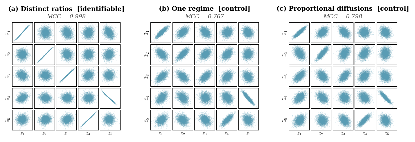
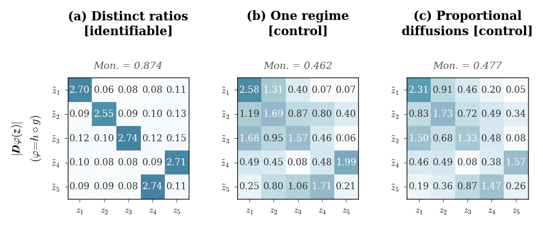
The \(d=7\) case uses the same construction with identical \(\lambda = 0.5\). The resulting drift matrix, rounded to two decimals, is \[A = \begin{pmatrix} -4.89 & 1.11 & -2.12 & -0.13 & 0.98 & -2.94 & 4.09 \\ 1.11 & -5.21 & -2.30 & -0.70 & 4.00 & -1.50 & 0.93 \\ -2.12 & -2.30 & -9.39 & -0.37 & -0.35 & -5.45 & 4.37 \\ -0.13 & -0.70 & -0.37 & -8.22 & 4.36 & -3.82 & -1.67 \\ 0.98 & 4.00 & -0.35 & 4.36 & -8.66 & 3.26 & -1.52 \\ -2.94 & -1.50 & -5.45 & -3.82 & 3.26 & -7.56 & 4.88 \\ 4.09 & 0.93 & 4.37 & -1.67 & -1.52 & 4.88 & -8.83 \end{pmatrix}.\]
Figures 6 and 7 show the \(d=7\) results. The same qualitative pattern holds: Distinct ratios achieves near-perfect disentanglement, while both controls show substantially less coordinate recovery.
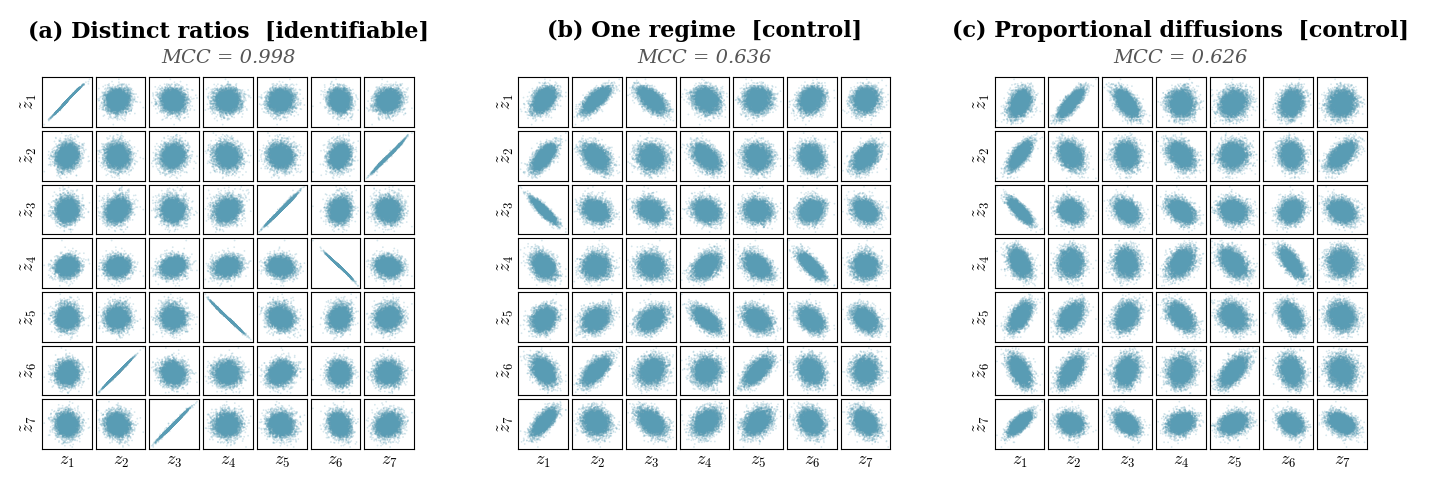
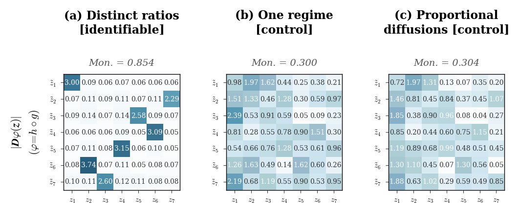
13.2 Sparse linear drift↩︎
The sparse linear experiments use an Ornstein–Uhlenbeck process with a sparse drift matrix \(A\) built from a directed cycle support. The nonzero off-diagonal support entries are placed at \((i,i+1)\) for \(i=1,\ldots,d-1\) and at \((d,1)\), and the drift matrix is constructed as \[A_{ii} = -\alpha, \qquad A_{ij} = \beta \, c_{ij} \;\text{if } \mathrm{adj}(i,j)=1, \qquad A_{ij} = 0 \;\text{otherwise},\] where \(\alpha = 1.0\), \(\beta = 1.5\), and \(c_{ij} \stackrel{\mathrm{iid}}{\sim} \mathrm{Uniform}(0.8, 1.2)\) with a fixed seed. The same \(A\) is shared across all training seeds and all three regime conditions.
For \(d=5\) the drift matrix, rounded to two decimals, is \[A = \begin{pmatrix} -1.00 & 1.77 & 0 & 0 & 0 \\ 0 & -1.00 & 1.72 & 0 & 0 \\ 0 & 0 & -1.00 & 1.33 & 0 \\ 0 & 0 & 0 & -1.00 & 1.37 \\ 1.57 & 0 & 0 & 0 & -1.00 \end{pmatrix}.\]
Figure 8 shows the pairwise scatter plots for the sparse linear \(d=5\) setting. Figure 9 displays the encoder Jacobian and graph recovery. Under Distinct ratios, the encoder inverts the mixing up to permutation and scaling, and the thresholded drift-Jacobian graph is recovered exactly (GMR \(=1\) for the representative seed).

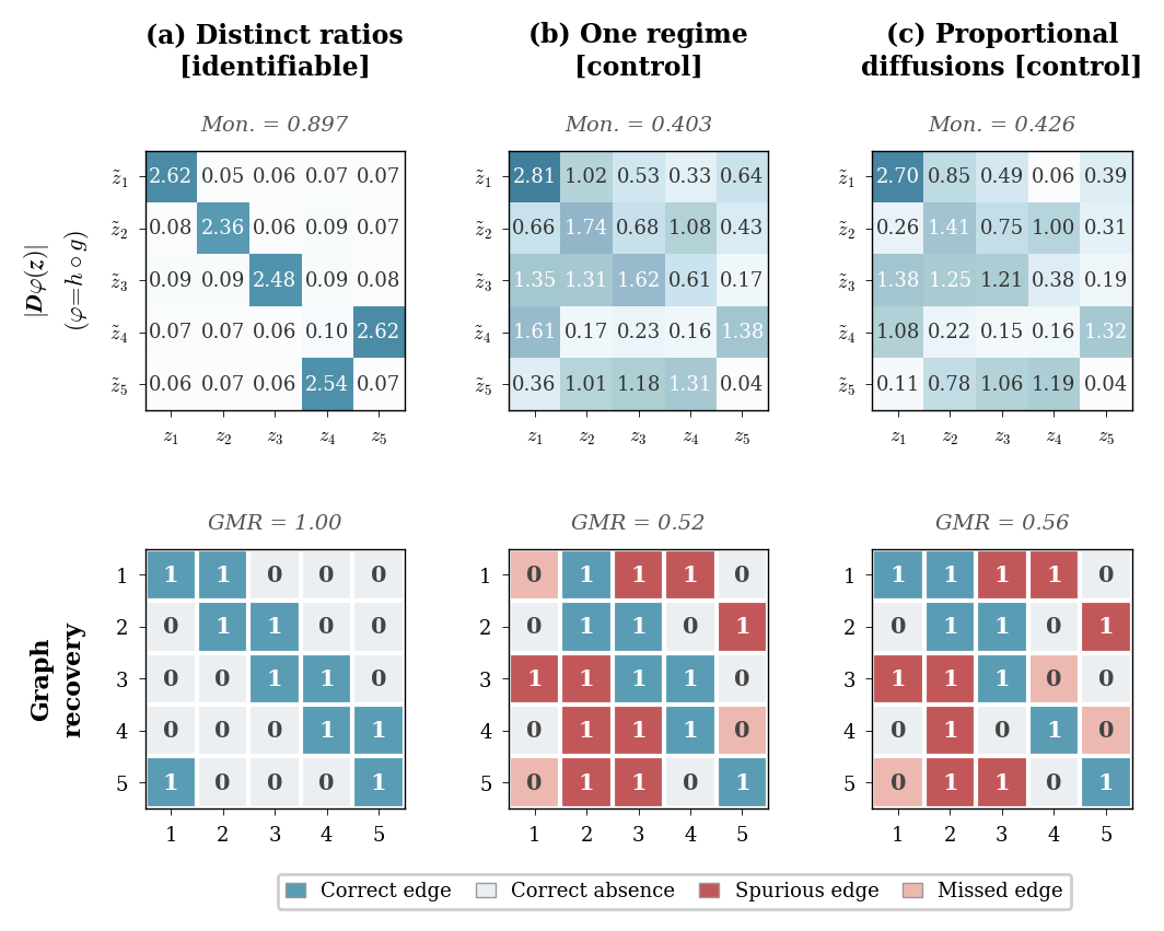
The \(d=7\) case uses the same construction. The drift matrix, rounded to two decimals, is \[A = \begin{pmatrix} -1.00 & 1.77 & 0 & 0 & 0 & 0 & 0 \\ 0 & -1.00 & 1.62 & 0 & 0 & 0 & 0 \\ 0 & 0 & -1.00 & 1.51 & 0 & 0 & 0 \\ 0 & 0 & 0 & -1.00 & 1.67 & 0 & 0 \\ 0 & 0 & 0 & 0 & -1.00 & 1.77 & 0 \\ 0 & 0 & 0 & 0 & 0 & -1.00 & 1.50 \\ 1.22 & 0 & 0 & 0 & 0 & 0 & -1.00 \end{pmatrix}.\]
Figures 10 and 11 show the corresponding results for \(d=7\). The same qualitative pattern holds: Distinct ratios gives near-monomial encoder Jacobians and near-perfect graph recovery, whereas the controls show mixed encoder Jacobians and lower GMR.
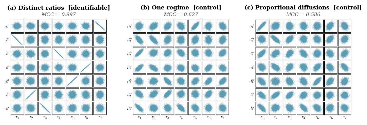
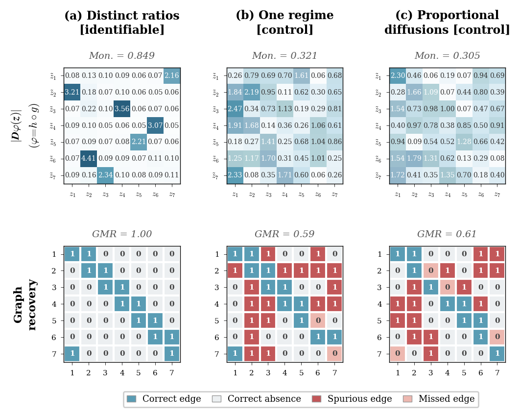
13.3 Nonlinear sparse drift↩︎
The nonlinear experiments use the same directed cycle support as the sparse linear case (Section 13.2), but replace the linear coupling with a \(\tanh\) nonlinearity. Concretely, the drift function is \[f_i(z) \;=\; -\alpha \, z_i \;+\; \beta \sum_{j:\,\mathrm{adj}(i,j)=1} c_{ij}\,\tanh(z_j),\] where \(\alpha = 1.0\) enforces mean-reversion along the diagonal and \(\beta = 1.5\) controls the coupling strength. The coefficients \(c_{ij}\) are drawn independently from \(\mathrm{Uniform}(0.8, 1.2)\) with a fixed seed and are nonzero only where the adjacency is \(1\). For \(d=5\) the nonzero coupling coefficients, rounded to two decimals, are \[c_{12} = 1.18,\quad c_{23} = 1.15,\quad c_{34} = 0.88,\quad c_{45} = 0.92,\quad c_{51} = 1.04.\] Here \(\mathrm{adj}(i,j)=1\) means that coordinate \(z_j\) enters the \(i\)th drift component \(f_i\).
For \(d=7\) the nonzero off-diagonal support entries are again placed at \((i,i+1)\) for \(i=1,\ldots,6\) and at \((7,1)\), and the nonzero coupling coefficients, rounded to two decimals, are \[c_{12} = 1.09,\quad c_{23} = 0.95,\quad c_{34} = 1.13,\quad c_{45} = 1.06,\quad c_{56} = 1.03,\quad c_{67} = 0.97,\quad c_{71} = 1.08.\] The Jacobian of \(f\) evaluated at the origin recovers the same sparse support pattern as in Section 13.2, but away from the origin the \(\tanh\) saturates, making the dynamics genuinely nonlinear.
For each fixed dimension, the same drift function is shared across the leaky-\(\tanh\) and LeakyReLU mixing experiments. The main text (Figures 1 and 2) reports the \(d=5\) results under leaky-\(\tanh\) mixing. Here we show the corresponding results under LeakyReLU mixing for both \(d=5\) and \(d=7\). All three regime conditions in each figure use the same representative training seed for a fair comparison. The identifiability gap is consistent with the leaky-\(\tanh\) results in the main text. Under Distinct ratios, the displayed run recovers clear coordinate alignment and a substantially more accurate thresholded graph; the controls show mixed coordinates and graph errors.
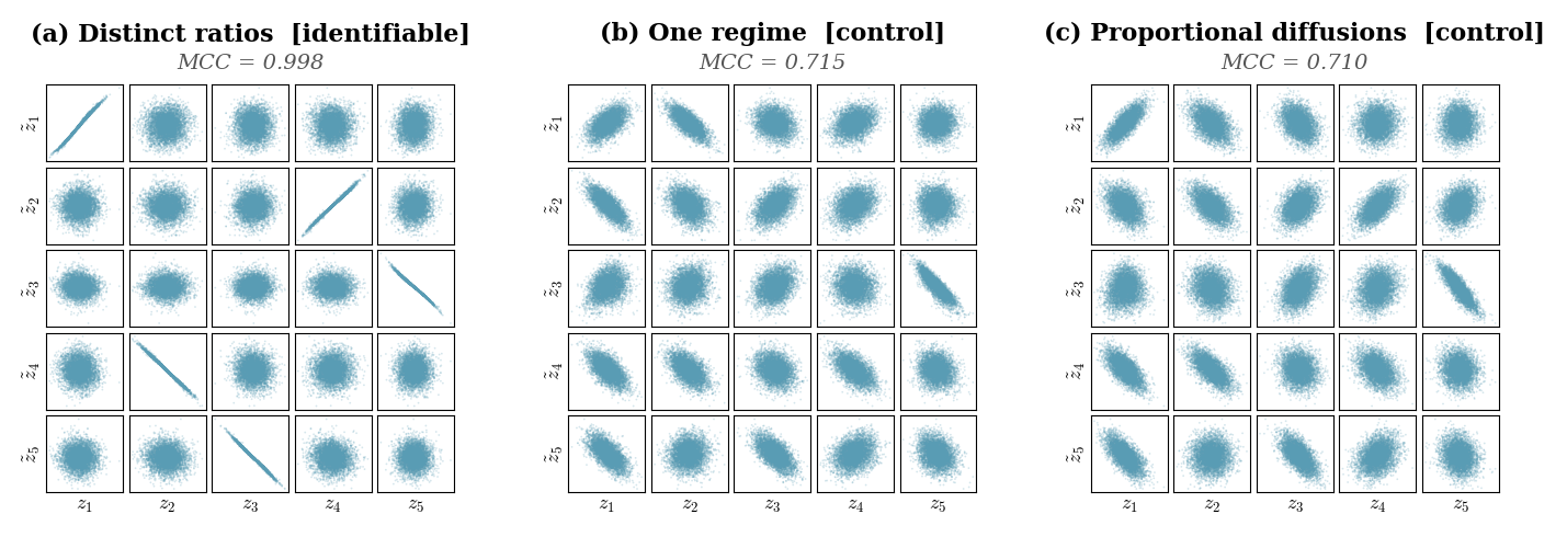
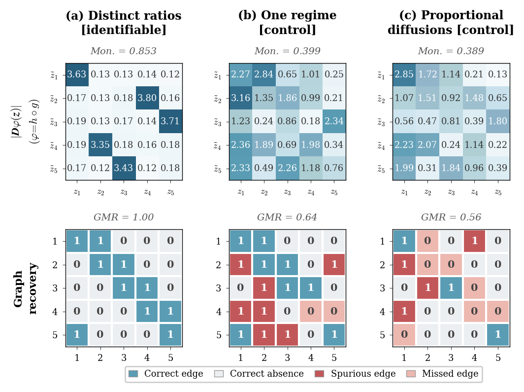
Figures 14 and 15 show the \(d=7\) results under LeakyReLU mixing. The identifiability gap remains clear: Distinct ratios achieves near-perfect disentanglement and high graph match rate, whereas both controls show weaker coordinate recovery and less reliable graph recovery.
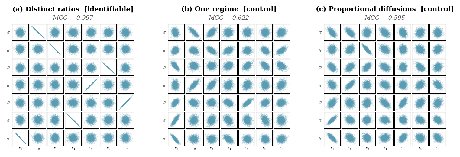
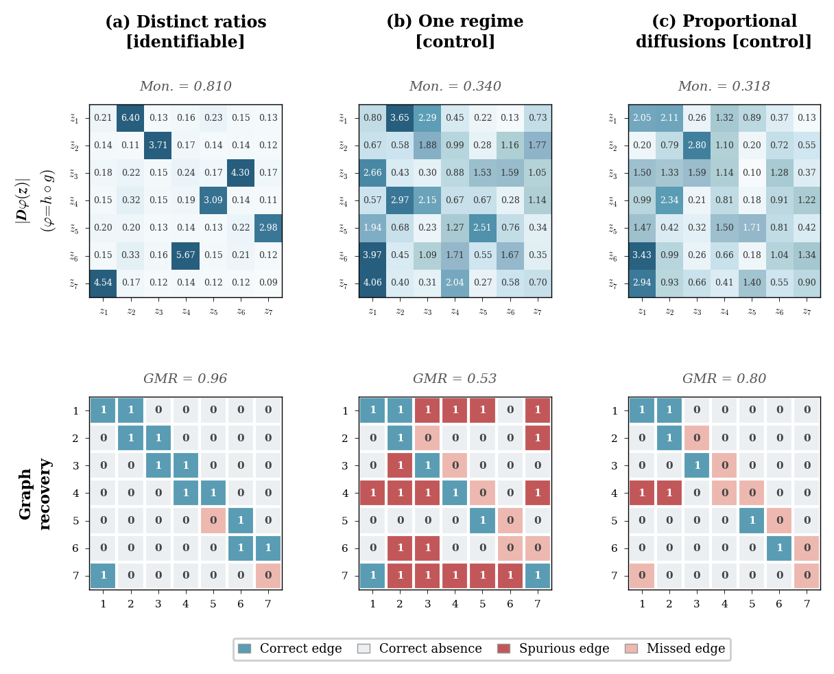
14 Real-world case study: Hardanger Bridge↩︎
This appendix gives the setup and diagnostics behind the Hardanger Bridge experiment reported in Section 5.2. The goal of this experiment is not to evaluate recovery against ground-truth latent coordinates, which are unavailable in the real bridge data. Instead, we test whether the TI-split two-regime construction produces a more reproducible latent representation and drift structure than controls that remove the turbulence-intensity (TI) contrast. The appendix first describes the data and training protocol, then reports cross-seed reproducibility, diffusion-fingerprint diagnostics, and a representative learned drift structure.
14.1 Dataset and regime construction↩︎
We use operational acceleration recordings from the Hardanger Bridge, a long-span suspension bridge monitored with wind and acceleration sensors [28], [29]. The dataset DOI/repository record lists a Creative Commons Attribution 4.0 International (CC BY 4.0) license [28]. The model receives only bridge-deck accelerometer channels as observations. Wind measurements are used only to construct regimes, not as model inputs.
To keep the shared-drift assumption physically meaningful, we restrict the data to a single mean-wind-speed bin, \(4\)–\(6\,\mathrm{m/s}\). Within this bin, each raw recording is divided into non-overlapping \(120\,\mathrm{s}\) sub-windows. For each sub-window we compute the turbulence intensity \[\mathrm{TI} = \frac{\mathrm{std}(\text{wind speed})}{\mathrm{mean}(\text{wind speed})}.\] The two regimes are then defined by a quantile split of TI: the bottom \(20\%\) of sub-windows form the low-TI regime and the top \(20\%\) form the high-TI regime; the middle \(60\%\) is discarded. This construction is the real-world analogue of the distinct-diffusion-regime condition in the synthetic experiments: the bridge dynamics are approximately shared within a matched wind speed bin, while turbulence intensity changes the stochastic excitation.
Table 8 summarizes the resulting dataset. The accelerometer signals are detrended, low-pass filtered at \(2.5\,\mathrm{Hz}\), resampled to \(10\,\mathrm{Hz}\), and standardized with one scaler fitted jointly across both regimes. The selected \(120\,\mathrm{s}\) sub-windows are then converted into overlapping \(12.8\,\mathrm{s}\) trajectory windows with \(6.4\,\mathrm{s}\) stride for training.
6pt
| Quantity | Value |
|---|---|
| Mean-wind-speed bin | \(4\)–\(6\,\mathrm{m/s}\) |
| Accelerometer channels | \(16\) bridge-deck channels |
| Regime statistic window | \(120\,\mathrm{s}\), non-overlapping |
| Low-TI threshold | \(0.0336\) |
| High-TI threshold | \(0.0794\) |
| Selected sub-windows | \(987\) low-TI and \(987\) high-TI |
| Trajectory window | \(12.8\,\mathrm{s}\) (\(128\) steps at \(\Delta t=0.1\)) |
| Trajectory stride | \(6.4\,\mathrm{s}\) |
| Training trajectories | \(16{,}779\) per regime |
| Input dimension / latent dimension | \(d_x=16\), \(d_z=5\) |
14.2 Training protocol and controls↩︎
We use the same two-stage estimator as in Section 4. The encoder is a three-layer MLP with hidden dimension \(64\), and the drift model is linear in the learned \(d_z=5\) coordinates. Both stages are trained for up to \(10{,}000\) epochs with early stopping patience \(100\). Stage 2 uses stride \(s=6\), sparse-Jacobian penalty \(\lambda_{\mathrm{sparse}}=1.0\), and graph threshold \(\tau=0.05\). All three regime constructions use the same list of ten random training seeds. The Hardanger runs use the same single-GPU compute setup as the simulation experiments in Appendix 12.4.
We compare three regime constructions:
TI-split regimes (ours): the bottom and top TI quantiles are used as two regimes.
One regime (control): the two TI groups are merged into a single environment. This preserves the total amount of data but removes regime-specific diffusion parameters.
Shuffled TI labels (control): the two TI groups are pooled and randomly re-split into two equally sized groups. This preserves the two-regime training format but destroys the turbulence-based contrast.
14.3 Evaluation metrics↩︎
Because ground-truth latent states are not available, we evaluate reproducibility across random seeds. For each seed, we encode the same set of \(5{,}000\) evaluation points. For every pair of seeds, we align learned coordinates by Hungarian matching on absolute correlation and compute the mean matched absolute correlation coefficient (MCC). We then use the same alignment to compare the thresholded drift-Jacobian graphs and report the graph match rate (GMR). With ten seeds, this gives \(\binom{10}{2}=45\) seed pairs. These are reproducibility diagnostics rather than accuracy metrics: high values mean that independent trainings recover compatible coordinate systems and drift graphs. As an auxiliary within-seed diagnostic, we also report the mean absolute off-diagonal correlation among learned latent coordinates; lower values indicate less redundant latent coordinates.
We also report diffusion-fingerprint diagnostics for the two-regime conditions. For parametric fingerprints, we use the learned diagonal variances \(\tilde{\sigma}_{e,k}^2\) from Stage 1 and compute \(r_k^{\mathrm{par}}=\tilde{\sigma}_{2,k}^2/\tilde{\sigma}_{1,k}^2\). For empirical fingerprints, we compute residual covariance matrices \(C_e\) after Stage 2 and use \(r_k^{\mathrm{emp}}=C_{2,kk}/C_{1,kk}\). Since the learned coordinates are identified only up to permutation and scaling, and since the sign of the log-ratio follows the internal regime ordering, we summarize contrast magnitude by \(|\log r_k|\) pooled over seeds and latent dimensions.
14.4 Cross-seed consistency↩︎
Table 9 expands the main-text result with descriptive standard deviations across seed pairs. TI-split regimes yield the highest latent reproducibility and the highest drift-graph reproducibility. The MCC gain is substantial relative to both controls: \(+0.146\) over One regime and \(+0.205\) over Shuffled TI labels. The same construction also gives the lowest mean latent off-diagonal correlation, suggesting that the learned coordinates are less redundant within each learned representation. Because the thresholded drift graphs are mostly diagonal with sparse off-diagonal edges, absolute GMR values can be helped by matching many absent edges; we therefore interpret the relative TI-split gain together with MCC and the diffusion fingerprints below.
4pt
| Regime construction | MCC \(\uparrow\) | GMR \(\uparrow\) | |
| offdiag.corr.\(\downarrow\) | |||
| TI-split regimes (ours) | \(\mathbf{0.806 \pm 0.061}\) | \(\mathbf{0.877 \pm 0.081}\) | \(\mathbf{0.182 \pm 0.022}\) |
| One regime (control) | \(0.660 \pm 0.051\) | \(0.813 \pm 0.077\) | \(0.250 \pm 0.040\) |
| Shuffled TI labels (control) | \(0.601 \pm 0.067\) | \(0.830 \pm 0.070\) | \(0.239 \pm 0.052\) |
14.5 Diffusion-fingerprint diagnostics↩︎
Table 10 shows that the TI-split regimes produce a strong learned diffusion contrast, whereas Shuffled TI labels collapse the fingerprint ratios to nearly one. This is the intended behavior of the control: it preserves the existence of two batches in the objective but removes the physical TI-based regime information. Thus the reproducibility gap in Table 9 is accompanied by the expected difference in learned diffusion fingerprints. Since Assumption (S4) requires latent coordinates to carry separating diffusion-ratio fingerprints across regimes, the large TI-split contrasts provide empirical support that the TI-based regime construction supplies the kind of diffusion variation required by the theory; the shuffled-label control does not. This is a diagnostic check rather than a formal verification of S4 in the absence of ground-truth latent coordinates.
The One-regime control is omitted from the fingerprint table because it has only one diffusion covariance and therefore no variance ratio.
4pt
| Regime construction | ||
| contrast \(\uparrow\) | ||
| contrast \(\uparrow\) | ||
| TI-split regimes (ours) | \(\mathbf{1.571 \pm 0.287}\) | \(\mathbf{0.797 \pm 0.150}\) |
| Shuffled TI labels (control) | \(0.009 \pm 0.005\) | \(0.003 \pm 0.002\) |
14.6 Representative learned structure↩︎
Figure 16 shows the learned drift Jacobians for a randomly selected seed, shared across the three regime constructions and ordered as in the main text. In each heatmap, row \(i\) corresponds to drift component \(\tilde{f}_{\psi,i}\) and column \(j\) corresponds to source coordinate \(\tilde{z}_j\); the plotted value is the evaluation mean of \(|\partial \tilde{f}_{\psi,i}/\partial \tilde{z}_j|\). Each panel is diagonal-dominant, but the off-diagonal structure differs across regime constructions. This is the qualitative pattern one would expect if the learned coordinates approximate a modal-like coordinate system for bridge vibrations: self-dynamics should dominate, while cross-coordinate effects should appear as a small number of structured couplings rather than as dense or scattered dependence. In this representative TI-split-regime run, the largest off-diagonal entries form a reciprocal pair between two learned coordinates: one drift component depends on the other coordinate with magnitude about \(0.48\), and the reverse dependence has magnitude about \(0.40\). A reciprocal pair of this kind is consistent with a learned two-dimensional dynamical subspace, as can arise from nearby vibration modes, non-proportional damping, aeroelastic or environmental coupling, or residual mixing in modal-like coordinates. By contrast, the controls under the same representative seed also contain off-diagonal entries, but these appear as more scattered one-way couplings across different coordinate pairs rather than as a single coherent coupled block. The TI-split structure is therefore more naturally aligned with this modal-like physical interpretation, while still serving only as an illustrative structural diagnostic that complements the aggregate reproducibility and fingerprint results above.
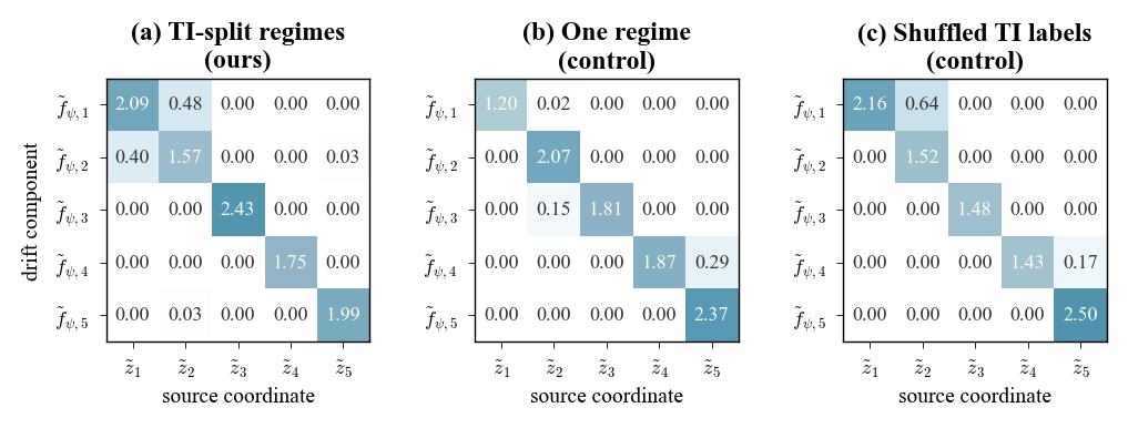
14.7 Limitations of the real-world diagnostic↩︎
This experiment should be read as a real-world diagnostic rather than a ground-truth recovery benchmark. The Hardanger data do not provide true latent coordinates or a true causal graph, so MCC and GMR measure cross-seed reproducibility after alignment, not absolute accuracy; absolute GMR values can also be influenced by matching many absent edges in sparse thresholded graphs. The diffusion-fingerprint ratios support the presence of TI-dependent diffusion variation, but they do not formally verify Assumption (S4) because the true latent coordinates and diffusion covariances are unobserved. Likewise, the modal-like interpretation of the representative drift Jacobian is not a substitute for external validation against finite-element models or modal analysis labels. Finally, the TI quantile split is a proxy for diffusion-regime variation. Its usefulness depends on maintaining enough stochastic-forcing contrast while keeping the deterministic structural dynamics approximately shared, exactly the tradeoff made explicit by the theory.