A fast sum-of-Gaussians algorithm for the high-dimensional fractional Fokker–Planck equation
January 01, 1970
Abstract
We present a fast, high-order algorithm for the free-space fractional Fokker–Planck equation (FFPE) in arbitrary spatial dimension. Its fundamental solution, corresponding to a Dirac-delta initial condition, is obtained from the explicit Fourier representation by applying a sum-of-Gaussians (SOG) approximation to the nonseparable stretched exponential, using its complete monotonicity as the Laplace transform of a one-sided \(\alpha\)-stable density. Each Gaussian term is an ordinary heat kernel and therefore factorizes across spatial coordinates. On a tensor-product grid, the separated form can be assembled in \(O(MdN)\) work and storage, rather than forming all \(O(N^d)\) grid values, where \(M\) is the number of Gaussian terms and \(N\) is the number of points per dimension. We prove an a priori error estimate for the pure-fractional fundamental solution and give a parameter-selection procedure for prescribed accuracy over specified ranges of space and time. In numerical experiments the method achieves more than ten digits of relative accuracy, with \(M\) growing only logarithmically in the inverse tolerance, and maintains this accuracy in dimensions up to \(d=10^{5}\). This exceeds the dimensions reached in comparable radial-quadrature tests, where the integrand becomes increasingly oscillatory as the dimension grows. Because the method represents the fundamental solution as a separated sum of heat kernels, any initial datum given as a finite sum of tensor products can be evolved in closed form using only one-dimensional convolutions. This yields a computable class of high-dimensional solutions that is amenable to error analysis, and tensor neural networks provide one possible way to construct such separated representations for more general data.
high-dimensional problems, sum-of-Gaussians approximation, Fokker–Planck equation, sparse grids, tensor neural networks, fast algorithms
35Q84, 34K37, 65D40, 68W25, 68W40
1 Introduction↩︎
The Fokker–Planck equation (FPE) provides a deterministic description of the time evolution of probability density functions for stochastic systems [1], [2], with applications in statistical mechanics, stochastic processes, mathematical finance, information theory, and machine learning [3]–[7]. In the classical regime, the underlying dynamics are typically driven by Gaussian white noise, leading to the well-known linear growth of mean-squared displacement, i.e., \(\langle |x|^2 \rangle \propto t\) [8]. However, many anomalous-transport models require non-Gaussian jump statistics with algebraic tails and a self-similar length scale that differs from the Brownian scale. In the spatially fractional model considered here, the Fourier symbol \(|\boldsymbol{k}|^{2\alpha}\) with \(0<\alpha<1\) corresponds to a symmetric stable process of index \(2\alpha\): the characteristic length grows like \(t^{1/(2\alpha)}\), while moments of order \(q\ge 2\alpha\) are infinite. Such heavy-tailed anomalous diffusion is modeled by the fractional Fokker–Planck equation (FFPE), where the classical Laplacian is replaced by a fractional Laplacian operator \((-\Delta)^\alpha\) [9], defined for \(\boldsymbol{x}\in \mathbb{R}^{d}\) through the Cauchy principal value \[\label{eq::fractional95operator} (-\Delta)^{\alpha}p(\boldsymbol{x})=\frac{2^{2\alpha}\Gamma(\alpha+d/2)}{\pi^{d/2}|\Gamma(-\alpha)|}\text{P.V.}\int_{\mathbb{R}^{d}}\frac{p(\boldsymbol{x})-p(\boldsymbol{y})}{|\boldsymbol{x}-\boldsymbol{y}|^{d+2\alpha}}\mathrm{d}\boldsymbol{y},\tag{1}\] where \(\Gamma(z)\) denotes the Gamma function.
The fractional Laplacian \((-\Delta)^\alpha\) makes the equation nonlocal and captures long-range jumps associated with Lévy stable processes [10]–[13]. We consider the following initial value problem for the high-dimensional FFPE: \[\label{eq::FFPE95formula} \begin{cases} \frac{\partial }{\partial t}p(\boldsymbol{x},t) = -\boldsymbol{b} \cdot \nabla p(\boldsymbol{x},t) + D_{o}\Delta p(\boldsymbol{x},t) - D_{f}(-\Delta)^{\alpha}p(\boldsymbol{x},t), \\ p(\boldsymbol{x},0) = \delta(\boldsymbol{x}-\boldsymbol{x}_{0}), \quad \boldsymbol{x} \in \mathbb{R}^{d}, \end{cases}\tag{2}\] where \(\boldsymbol{b} \in \mathbb{R}^d\) is the drift vector, and \(D_o \ge 0\) and \(D_f > 0\) are the ordinary and fractional diffusion coefficients. The solution of 2 is the fundamental solution (Green’s function) of the FFPE; by linearity it determines, through convolution, the solution for a general initial datum. We therefore take the Dirac-delta case as the basic building block and use the same representation for separated initial data in high dimension.
Numerical treatment of Eq. 2 in high dimensions poses substantial mathematical and computational challenges. First, traditional grid-based methods, such as finite difference or finite element schemes, suffer from the curse of dimensionality: the degrees of freedom grow exponentially with the dimension \(d\) [14], [15]. Second, the nonlocality of \((-\Delta)^\alpha\) leads to dense discretized operators, which are costly for large-scale problems. Monte Carlo sampling and deep-learning-based solvers [16], [17] avoid full grids, but the Dirac-delta initial condition and slow convergence can still be limiting factors [15]. Recent methods based on functional hierarchical tensors [18] and fundamental-solution integrals [19] improve this situation. In particular, Ye et al. [19] reduce the free-space FFPE with Dirac-delta initial data to a one-dimensional radial integral that is evaluated to high precision in low to moderate dimensions. That approach relies on radial quadrature: as \(d\) increases, the Bessel order \((d-2)/2\) and the power \(r^{d/2}\) in the integrand both grow, making the integrand more oscillatory and increasing its dynamic range; the method is demonstrated up to \(d=29\). This motivates the separable representation developed here, which is aimed at higher dimensions and at separated initial data. The two approaches are complementary: the radial integral remains effective in low to moderate dimension, whereas the present method is designed for high-dimensional separated representations.
To address these challenges, we develop a fast algorithm based on a sum-of-Gaussians (SOG) approximation of the fundamental solution. The fractional operator enters the Fourier-space solution only through the stretched-exponential factor \(\exp(-D_ft|\boldsymbol{k}|^{2\alpha})\), the one piece that does not factorize across coordinates. Because this factor is completely monotone [20], it is the Laplace transform of a one-sided \(\alpha\)-stable density, and a trapezoidal discretization of that representation turns it into a sum of Gaussians – each an ordinary heat kernel that factorizes across dimensions. The FFPE thus reduces to a short separated sum of decoupled heat solutions. On a tensor-product grid, its one-dimensional factors are assembled in \(O(MdN)\) work and storage rather than forming \(O(N^d)\) dense grid values, where \(M\) is the number of Gaussians and \(N\) the number of points per dimension.
This construction is accurate, admits a rigorous error analysis, and extends naturally to low-rank summation of separated initial data. We give a rigorous a priori error analysis for the pure-fractional kernel that fixes the quadrature step and truncation for any prescribed tolerance, with convergence governed by a complex-plane bound on the stable density. For prescribed physical windows, the same scaled formulation gives a domain-adapted parameter choice for all \(\alpha\in(0,1)\) and includes the ordinary-diffusion case \(D_o>0\); when \(\alpha=1/2\), a closed-form identity for the trapezoidal error provides an additional analytic reference. In numerical experiments the method attains more than ten digits of relative accuracy with \(M\) growing only logarithmically in the inverse tolerance, and sustains this accuracy up to \(d=10^{5}\), well beyond the dimensions reachable by radial-quadrature methods. Because the relative error obeys a self-similar scaling, a single approximation sized at the smallest time serves an entire space-time window and avoids the small-time, high-dimensional loss of accuracy observed for direct quadrature [19]. Finally, since the method approximates the fundamental solution by a separated sum of Gaussians, any initial datum written as a sum of tensor products evolves in closed form through one-dimensional convolutions alone – a class of high-dimensional functions that is computable and amenable to error analysis [21]–[23]. Sparse-grid approximation methods [24], [25] and tensor neural networks [26]–[28] provide complementary ways to construct reduced representations for more general data.
Gaussian-sum approximations also arise in other high-dimensional PDE contexts. For example, in time-independent many-electron Schrödinger eigenvalue problems, mixed-derivative regularity [29] provides analytic support for sparse-grid approximations, and sparse-grid methods have been developed for the Schrödinger equation [30]. The pairwise Coulomb kernel \(1/|\boldsymbol{r}_i-\boldsymbol{r}_j|\), which is nonseparable in the electronic coordinates, admits accurate SOG approximations; after expansion into Gaussian factors, it is compatible with tensor-product integration and tensor neural network representations [31], [32]. For high-dimensional evolution problems, the same separability mechanism is relevant whenever a Fourier-space propagator, or a linear subproblem arising from time discretization, admits an accurate Gaussian-sum representation. For many nonlinear evolution equations, an unconditionally energy-stable scalar auxiliary variable (SAV) temporal discretization reduces each time step to a linear problem with known source terms [33]. If the resulting linear subproblem has a constant-coefficient solution operator that admits an accurate and efficient Gaussian-sum representation, the framework developed here extends naturally to such problems. These connections motivate SOG approximations as building blocks for separable representations in high-dimensional PDEs, although the analysis below is restricted to the FFPE fundamental solution.
The remainder of this paper is organized as follows. In 2, we review the mathematical preliminaries, including Fourier transforms, the theory of completely monotone functions, and properties of the stretched exponential function. In 3, we detail the SOG algorithm and provide its rigorous error estimate. Numerical experiments assessing the performance of the proposed solver are presented in 4, followed by concluding remarks in 5.
2 Preliminaries↩︎
2.1 Fourier transform↩︎
For a function \(f\in L^{1}(\mathbb{R}^{d})\cap L^{2}(\mathbb{R}^{d})\) we define its Fourier transform by \[\widehat{f}(\boldsymbol{k})=\mathcal{F}[f](\boldsymbol{k})=\int_{\mathbb{R}^{d}} f(\boldsymbol{x})\,e^{-i\,\boldsymbol{k}\cdot\boldsymbol{x}}\,\mathrm{d}\boldsymbol{x}, \qquad \boldsymbol{k}\in\mathbb{R}^{d},\] and the inverse Fourier transform by \[f(\boldsymbol{x})=\mathcal{F}^{-1}[\widehat{f}](\boldsymbol{x})=\frac{1}{(2\pi)^d}\int_{\mathbb{R}^{d}} \widehat{f}(\boldsymbol{k})\,e^{i\,\boldsymbol{k}\cdot\boldsymbol{x}}\,\mathrm{d}\boldsymbol{k}, \qquad \boldsymbol{x}\in\mathbb{R}^{d}.\] If \(f\) is radial, i.e.\(f(\boldsymbol{x})=f(r)\) with \(r=\sqrt{x_{1}^{2}+\dots+x_{d}^{2}}\), its Fourier transform is again radial. In this case, the radial Fourier transform (i.e., the Hankel transform) pairs are \[\begin{align} \widehat{f}(k)&=\frac{(2\pi)^{d/2}}{k^{(d-2)/2}} \int_{0}^{\infty} f(r)\,r^{\frac{d}{2}} J_{\frac{d-2}{2}}(kr)\,\mathrm{d}r,\\ f(r) &=\frac{1}{(2\pi)^{d/2} r^{(d-2)/2}} \int_{0}^{\infty} \widehat{f}(k)\,k^{\frac{d}{2}} J_{\frac{d-2}{2}}(kr)\,\mathrm{d}k, \end{align}\] where \(J_{\nu}\) is the Bessel function of the first kind of order \(\nu\). Finally, for a sufficiently regular and rapidly decaying \(f\) the Poisson summation formula [34] links sums over the integer lattice to sums over its dual: \[h\sum_{n=-\infty}^{\infty} f(hn + a) = \sum_{m=-\infty}^{\infty} e^{i \frac{2\pi m a}{h}} \widehat{f}\left(\frac{2\pi m}{h}\right), \label{eq:poissonsf}\tag{3}\] providing a powerful bridge between spatial and frequency-domain information.
2.2 Completely monotone functions↩︎
Definition 1 (Completely monotone function). A function \(f: (0, \infty) \to \mathbb{R}\) is completely monotone if \(f\in C^\infty\) and \[(-1)^n f^{(n)}(x)\ge0\] for all nonnegative integers \(n\) and all \(x\in(0,\infty)\).
The following result, Bernstein’s theorem, provides a crucial integral representation that is often used as an alternative definition (see, for example, [35]).
Lemma 1 (Bernstein’s theorem). A function \(f: (0, \infty) \to \mathbb{R}\) is completely monotone if and only if it is the Laplace transform of a nonnegative Borel measure \(\mu\) on \([0,\infty)\): \[f(x)=\int_0^\infty e^{-xt}\,\mathrm{d}\mu(t).\] If the measure has a density \(\rho(t)\ge0\), this representation becomes \[f(x)=\int_0^\infty e^{-xt}\rho(t)\,\mathrm{d}t.\]
2.3 Properties of the stretched exponential and its inverse Laplace transform↩︎
The function \[f(x)=e^{-x^\alpha}, \qquad 0<\alpha<1, \label{eq:kwwfun}\tag{4}\] also known as the stretched exponential or Kohlrausch–Williams–Watts (KWW) function, possesses several important properties.
Lemma 2. The stretched exponential function is completely monotone on \((0,\infty)\) and has the integral representation \[e^{-x^{\alpha}} = \int_0^{\infty} e^{-xt}\rho_\alpha(t)\,\mathrm{d}t, \label{eq:kwwfunrep}\qquad{(1)}\] where \(\rho_\alpha\) is the probability density function (PDF) of a standard one-sided stable distribution (also called the one-sided Lévy \(\alpha\)-stable distribution).
Proof. The fact that the stretched exponential function is completely monotone can be shown via direct calculation of \(f^{(n)}(x)\). The integral representation ?? can be found, say, in [20]. ◻
The following properties of \(\rho_{\alpha}\) can be found in [36].
Lemma 3.
For \(t>0\), \(\rho_\alpha\) admits an integral representation \[\label{eq::Levy} \rho_\alpha(t)=\frac{1}{\pi}\int_{0}^{+\infty}e^{-\cos(\alpha\pi)u^{\alpha}}e^{-ut}\sin(\sin(\alpha\pi)u^{\alpha})\mathrm{d}u.\qquad{(2)}\]
For \(t > 1\), \(\rho_\alpha\) admits the following series expansion \[\rho_\alpha(t) = \frac{1}{\pi} \sum_{n=1}^{\infty} \frac{(-1)^{n-1}}{n!} \sin(\pi n \alpha) \Gamma(n\alpha+1) t^{-(n\alpha+1)}\le C_\alpha t^{-(1+\alpha)}, \label{eq:seriesexpansion}\qquad{(3)}\] where \(C_\alpha\) is a positive constant depending on \(\alpha\) (bounded on compact subintervals of \((0,1)\)).
As \(t \to 0^+\), \(\rho_\alpha\) has the asymptotic expansion: \[\rho_\alpha(t) = C t^{\frac{\alpha-2}{2(1-\alpha)}} \exp\left(-D t^{-\frac{\alpha}{1-\alpha}}\right)\left( \sum_{k=0}^{\infty} a_k t^{\frac{k\alpha}{1-\alpha}} \right) \label{eq:asympexpansion}\qquad{(4)}\] where the constants \(C\) and \(D\) are positive and depend on \(\alpha\): \[C = \frac{1}{\sqrt{2\pi (1-\alpha)}} \alpha^{\frac{1}{2(1-\alpha)}}, \qquad D = (1-\alpha) \alpha^{\frac{\alpha}{1-\alpha}},\] and the first two coefficients \(a_k\), \(k=0,1\) are given by: \[a_0 = 1, \qquad a_1 = \frac{(2-\alpha)(1-2\alpha)}{24\alpha(1-\alpha)} \alpha^{-\frac{\alpha}{1-\alpha}}.\] Moreover, the estimate \[\rho_\alpha(t)\le A_\alpha t^{-\gamma}\exp(-D t^{-\frac{\alpha}{1-\alpha}})\] holds with a constant \(A_\alpha\) that has only an \(O(1/\sqrt{1-\alpha})\) singularity as \(\alpha\rightarrow 1^{-}\), where \(\gamma=(2-\alpha)/(2-2\alpha)\).
3 A fast sum-of-Gaussians FFPE solver↩︎
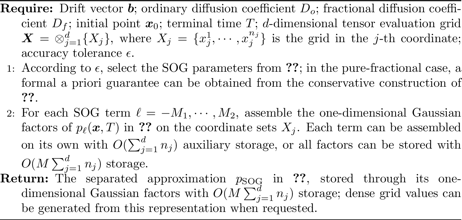
In this section, we present a fast algorithm for solving the FFPE 2 . By combining the radial Fourier-integral representation of the FFPE solution with a sum-of-Gaussians (SOG) approximation of the stretched exponential, the proposed method reduces the anomalous-diffusion solution to a sum of heat-equation solutions with closed-form expressions, thereby achieving a computational cost that grows linearly with the dimension.
3.1 SOE approximation of the stretched exponential function↩︎
We approximate the stretched exponential by a sum of exponentials (SOE), \[e^{-x^{\alpha}} \approx \sum_{\ell=-M_1}^{M_2} w_\ell e^{-s_\ell x}, \qquad x\in [\delta,R]. \label{eq:soeappr}\tag{5}\] Our starting point is the integral representation ?? . Applying the change of variables \(t=e^{u}\) to ?? , we obtain \[e^{-x^{\alpha}} = \int_{-\infty}^{\infty} e^{-x e^u+u}\rho_\alpha(e^u)\mathrm{d}u. \label{eq:kwwfunrep2}\tag{6}\] The integrand decays rapidly to zero as \(u\to\pm\infty\), so the trapezoidal rule converges exponentially fast [37], and the nodes \(s_\ell\) and weights \(w_\ell\) in 5 are given by \[s_\ell = e^{h\ell}, \qquad w_\ell = h s_\ell \rho_\alpha(s_\ell),\] where \(h>0\) is the step size in the trapezoidal rule.
We analyze the approximation error of 5 . We record the asymptotic magnitude of the Gamma function for a complex argument (Lemma 4, used in the parameter selection of 3.4); its proof is given in the appendix of [38].
Lemma 4. For fixed \(x\in \mathbb{R}\), the Gamma function satisfies \[\label{eq::Gamma} \left|\Gamma(x+iy)\right|\simeq (2\pi)^{1/2}(x^2+y^2)^{\frac{2x-1}{4}}e^{-\frac{\pi}{2}|y|}\qquad{(5)}\] as \(|y|\rightarrow \infty\).
We first analyze the discretization error of the (infinite) trapezoidal rule \[\label{eq::SOE} \begin{align} e^{-x^{\alpha}}&\approx \sum_{\ell=-\infty}^{+\infty}w_\ell e^{-s_\ell x}. \end{align}\tag{7}\]
Theorem 1. Let \(\alpha\in(0,1)\) and \(0<\epsilon_{\emph{SOE}}\le 1\), and set \(\theta=-(1-\alpha)\theta_{*}\) with \(\theta_{*}=\arctan(1/9)\). If the step size \(h\) satisfies \[\label{eq::h95select} h\le \frac{2\pi(1-\alpha)\theta_*}{\log(1+2I_\alpha/\epsilon_{\emph{SOE}})}\qquad{(6)}\] where \[I_{\alpha}:=\int_{0}^{\infty}|\rho_\alpha(re^{i\theta})|\mathrm{d}r,\] then \[\label{eq::error} \left|e^{-x^{\alpha}}-\sum_{\ell=-\infty}^{+\infty}w_\ell e^{-s_\ell \cdot x}\right|\le \epsilon_{\emph{SOE}},\qquad{(7)}\] holds for all \(x\in [0,+\infty)\).
Proof. Combining the Poisson summation formula 3 and the fact that \(\widehat{f}(0) = \int_\mathbb{R} f(u)du\), we obtain \[\label{eq::poisson} \left|\int_{\mathbb{R}}f(u)\mathrm{d}u-h\sum_{n\in \mathbb{Z}}f(nh)\right|\le \sum_{m\neq 0}\left|\widehat{f}\left(\frac{2\pi m}{h}\right)\right|,\tag{8}\] We now apply the above inequality to the integral representation 6 of the stretched exponential, i.e., \(f(u)=e^{u}\rho_\alpha(e^{u})e^{-xe^{u}}\). The error bound on the right-hand side of 8 is determined by the decay rate of \(\widehat{f}\). We have \[\label{eq::f95Fourier} \begin{align} \widehat{f}(k)&=\int_{-\infty}^{+\infty}e^{u}\rho_\alpha(e^{u})e^{-xe^{u}}e^{-iku}\mathrm{d}u\\ &=\int_{0}^{+\infty}e^{-xt}\rho_{\alpha}(t)t^{-ik}\mathrm{d}t.\\ \end{align}\tag{9}\] Let us consider the asymptotic approximation of the integral in 9 . We transform the integral path to \(C_\theta=\{re^{i\theta},r\in[0,+\infty)\}\). By Cauchy’s theorem, for a complex function \(g(z)\), if the angular region between \(C_0\) and \(C_\theta\) contains no singularity, then \[\int_{C_0}g(z)\mathrm{d}z=\int_{C_\theta}g(z)\mathrm{d}z.\] Since \(|\theta|\le \pi(1-\alpha)/2\), one then derives that \[\label{eq::Int95trans95calc} \begin{align} \widehat{f}(k) &=\int_{0}^{+\infty}e^{-xt}\rho_{\alpha}(t)t^{-ik}\mathrm{d}t,\\ &=\int_{0}^{+\infty}e^{-xre^{i\theta}}\rho_{\alpha}(re^{i\theta})r^{-ik}e^{\theta k}\mathrm{d}r\\ &=e^{\theta k}\int_{0}^{+\infty}e^{-xre^{i\theta}}\rho_{\alpha}(re^{i\theta})r^{-ik}\mathrm{d}r. \end{align}\tag{10}\] We choose the rotation opposite to the sign of \(k\), i.e. \(\theta=-\operatorname{sign}(k)\,\theta_{*}(1-\alpha)\), which lies in the sector of analyticity since \(\theta_{*}(1-\alpha)<\pi(1-\alpha)/2\). Because \(x\ge 0\) and \(\cos\theta>0\) give \(|e^{-xre^{i\theta}}|=e^{-xr\cos\theta}\le 1\), and \(|r^{-ik}|=1\), the rotated integral in 10 is bounded in modulus by \(\int_{0}^{\infty}|\rho_{\alpha}(re^{i\theta})|\mathrm{d}r\). Moreover, since \(\rho_\alpha\) is real on the positive axis, the reflection \(\rho_\alpha(\bar z)=\overline{\rho_\alpha(z)}\) shows that this integral takes the same value \(I_\alpha\) for \(+\theta\) and \(-\theta\). With \(e^{\theta k}=e^{-(1-\alpha)\theta_{*}|k|}\) for this sign choice, one deduces the convergence rate with respect to mode \(k\) that \[\label{eq::conv95rate95k} |\widehat{f}(k)|\le I_{\alpha} e^{-(1-\alpha)\theta_{*} |k|}.\tag{11}\] Substituting 11 into 8 , one has \[\label{eq::approx95error} \begin{align} \left|\int_{\mathbb{R}}f(u)\mathrm{d}u-h\sum_{n\in \mathbb{Z}}f(nh)\right|&\le \sum_{m\neq 0} I_\alpha e^{-2\pi(1-\alpha)\theta_{*}|m|/h}\\ &\le 2I_\alpha e^{-2\pi(1-\alpha)\theta_{*}/h}\frac{1}{1-e^{-2\pi(1-\alpha)\theta_{*}/h}}\\ &\le \epsilon_{\text{SOE}}. \end{align}\tag{12}\] ◻
Theorem 1 bounds the discretization error of the infinite rule uniformly on \([0,+\infty)\). Truncating the series to \(\ell\in[-M_1,M_2]\), as in 5 , restricts the accurate range to the finite window \([\delta,R]\), whose endpoints are governed by the extreme retained nodes: since a single term \(e^{-s_\ell x}\) acts on the scale \(x\sim s_\ell^{-1}\), the largest node \(s_{M_2}=e^{hM_2}\) sets the lower limit \(\delta\sim s_{M_2}^{-1}\) and the smallest node \(s_{-M_1}=e^{-hM_1}\) the upper limit \(R\sim s_{-M_1}^{-1}\). The truncation indices \(M_1,M_2\) are chosen in 3.3 to meet the target tolerance.
Theorem 2 provides a uniform bound of \(I_\alpha\).
Theorem 2. For \(\alpha\in(0,1)\) and \(\theta=\pm(1-\alpha)\theta_{*}\), there is a universal constant \(C_I\), independent of \(\alpha\), such that \[\label{eq::I95alpha95upper} I_\alpha=\int_0^\infty |\rho_\alpha(re^{i\theta})|\,\mathrm{d}r \le C_I\left(\frac{1}{\alpha}+\frac{1}{1-\alpha}\right).\qquad{(8)}\] More precisely, if \(I_\alpha^1\) and \(I_\alpha^2\) denote the contributions from \(r\in(0,1)\) and \(r\in(1,\infty)\), then \[I_\alpha^1\le \begin{cases} C_I/\alpha, & 0<\alpha\le 1/2,\\[2mm] C_I\log\!\bigl(e/(1-\alpha)\bigr), & 1/2\le \alpha<1, \end{cases} \qquad I_\alpha^2\le C_I\left(\frac{1}{\alpha}+\frac{1}{1-\alpha}\right).\]
The detailed proof is provided in Appendices 6 and 7. The estimate in ?? shows only mild endpoint singularities. The large factor that appears in a direct pointwise bound for \(|\rho_\alpha(z)|\) near \(\alpha=1\) is not intrinsic to \(I_\alpha\); in the proof of 7 the compact part is integrated in the radial variable before the saddle-contour integral is estimated, which preserves the cancellation in the phase. At \(\alpha=1\) the representing measure degenerates to a Dirac mass at \(z=1\), while the limit \(\alpha\to0^+\) is also degenerate and is no longer described by a regular probability density on \((0,\infty)\). Accordingly, endpoint regimes still require care in numerical density evaluation, but the contour constant entering the trapezoidal error does not grow like \(c^{1/(1-\alpha)}\).
3.2 The SOG approximation of the solution↩︎
Taking the Fourier transform of 2 with respect to the space variable \(\boldsymbol{x}\in \mathbb{R}^d\), we obtain \[\label{eq::FFPE95Fourier} \left\{\begin{align} &\frac{\partial}{\partial t}\widehat{p}(\boldsymbol{k}, t) =-i(\boldsymbol{k}\cdot\boldsymbol{b}) \widehat{p}(\boldsymbol{k}, t)-D_{\mathrm{o}}|\boldsymbol{k}|^2 \widehat{p}(\boldsymbol{k}, t)-D_{\mathrm{f}}|\boldsymbol{k}|^{2 \alpha} \widehat{p}(\boldsymbol{k}, t) \\ &\widehat{p}(\boldsymbol{k}, 0) =\exp \left(-i\boldsymbol{k}\cdot\boldsymbol{x}_0\right), \end{align}\right.\tag{13}\] which can be explicitly solved with \[\label{eq::p95hat95explicit} \widehat{p}(\boldsymbol{k}, t)=e^{-i\boldsymbol{k}\cdot\boldsymbol{x}_0^t}e^{-(D_o|\boldsymbol{k}|^2+D_f|\boldsymbol{k}|^{2\alpha})t},\quad \boldsymbol{x}_0^t:=\boldsymbol{x}_0+\boldsymbol{b}t.\tag{14}\] By the inverse Fourier transform, we have \[\label{eq::p95intergral} p(\boldsymbol{x},t)=\frac{1}{(2\pi)^d}\int_{\mathbb{R}^d}e^{i\boldsymbol{k}\cdot(\boldsymbol{x}-\boldsymbol{x}_0^t)}e^{-(D_o|\boldsymbol{k}|^2+D_f|\boldsymbol{k}|^{2\alpha})t}\mathrm{d}\boldsymbol{k}.\tag{15}\] Since the factor \(\exp(-(D_o|\boldsymbol{k}|^2+D_f|\boldsymbol{k}|^{2\alpha})t)\) is radially symmetric and hence invariant under coordinate rotations, we choose a new orthogonal coordinate frame \((\boldsymbol{e}_1,\cdots,\boldsymbol{e}_d)\) such that \(\boldsymbol{x}-\boldsymbol{x}_0^{t}\) lies along the first coordinate axis, that is, \(\boldsymbol{x}-\boldsymbol{x}_0^{t}=y\boldsymbol{e}_1\) with the direction vector \(|\boldsymbol{e}_1|=1\). For \(d\ge2\) and \(y>0\), by performing a \(d\)-dimensional spherical coordinate transformation \((k_1,k_2,\cdots,k_d)\rightarrow (r,\theta_1,\theta_2,\cdots,\theta_{d-1})\), the integral in 15 is equivalent to \[\label{eq::p95int95equiv} p(\boldsymbol{x},t)=\frac{\int_0^\pi \sin ^{d-2}(\theta) \int_0^{\infty} r^{d-1} \cos (\cos (\theta) y r) e^{-(D_or^2+D_f r^{2\alpha})t} \mathrm{d}r \mathrm{d} \theta}{2^{d-1}\pi^{\frac{d+1}{2}}\Gamma(\frac{d-1}{2})}\tag{16}\] where \(\Gamma(\cdot)\) denotes the Gamma function, and \(\theta\) abbreviates the first angular coordinate \(\theta_1\). Performing the angular integration for \(y\neq0\), and evaluating 15 directly for \(y=0\), gives the explicit radial integral expression [19] \[\label{eq::int95expression} p(\boldsymbol{x},t)= \left\{ \begin{align} &\frac{1}{y^{\frac{d-2}{2}}}\int_0^{\infty}\left(\frac{r}{2\pi}\right)^{\frac{d}{2}}J_{\frac{d-2}{2}}(yr)\exp(-(D_or^2+D_fr^{2\alpha})t)\mathrm{d}r,\;y\neq 0\\ &\frac{2^{1-d}}{\pi^{d/2}\Gamma\left(d/2\right)}\int_0^{\infty}r^{d-1}\exp(-(D_or^2+D_fr^{2\alpha})t)\mathrm{d}r,\;y=0, \end{align} \right.\tag{17}\] where \(J_\nu(\cdot)\) represents the \(\nu\)-th Bessel function of the first kind \[\label{eq::Bessel} J_\nu(z)=\frac{(z/2)^{\nu}}{\pi^{1/2}\Gamma(\nu+1/2)}\int_0^{\pi}\sin^{2\nu}(\theta)\cos(\cos(\theta)z)\mathrm{d}\theta.\tag{18}\] For a fixed terminal time \(T > 0\) and \(t\in[0,T]\), we apply the SOE expansion 5 to the fractional factor in \(\widehat{p}(\boldsymbol{k},t)\), namely \(e^{-D_ft|\boldsymbol{k}|^{2\alpha}}=e^{-x^{\alpha}}\) with \(x=(D_ft)^{1/\alpha}|\boldsymbol{k}|^2\), giving the sum-of-Gaussians (SOG) approximation \[\label{eq::SOG95approx} \widehat{p}(\boldsymbol{k}, t)\approx\widehat{p}_{\text{SOG}}(\boldsymbol{k},t)=\sum_{\ell=-M_1}^{M_2}w_\ell e^{-i\boldsymbol{k}\cdot\boldsymbol{x}_0^t}e^{-[D_ot+s_\ell(D_ft)^{1/\alpha}]|\boldsymbol{k}|^2}\tag{19}\] In real space, this procedure is equivalent to approximating the true solution \(p(\boldsymbol{x}, T)\) through a linear superposition of ordinary diffusion kernels. Specifically, this approximation is formulated as \[\label{eq::p95approx} p(\boldsymbol{x},T)\approx p_{\text{SOG}}(\boldsymbol{x},T):=\sum_{\ell=-M_1}^{M_2}w_\ell p_\ell(\boldsymbol{x},T),\tag{20}\] where \(p_\ell(\boldsymbol{x},T)\) is the solution to the following heat equation \[\label{eq::heat} \left\{ \begin{align} \frac{\partial}{\partial t}p_\ell(\boldsymbol{x},t)&=-\boldsymbol{b}\cdot\nabla p_\ell(\boldsymbol{x},t)+\left(D_{o}+\frac{s_\ell D_f}{\alpha} (D_ft)^{\frac{1}{\alpha}-1}\right)\Delta p_\ell(\boldsymbol{x},t)\\ p_\ell(\boldsymbol{x},0)&=\delta_{\boldsymbol{x}_0}(\boldsymbol{x}). \end{align} \right.\tag{21}\] The exact solution of 21 reads \[\label{eq::Heat95explicit} p_\ell(\boldsymbol{x},T)=\frac{1}{(4\pi C_\ell^{T})^{d/2}}\exp\left(-\frac{y^2}{4C_\ell^{T}}\right),\tag{22}\] where \(C_\ell^{T}:=D_oT+s_\ell (D_fT)^{1/\alpha}\) is the \(\ell\)-th ordinary diffusion constant in the SOG approximation.
Therefore, on a tensor-product observation grid \(\boldsymbol{X}=\otimes_{j=1}^d X_j\), each kernel \(p_\ell\) in 22 is represented by its one-dimensional Gaussian factors. Assembling the factors for one term costs \(O(\sum_{j=1}^d n_j)\) work and storage, and assembling all factors costs \(O(M\sum_{j=1}^d n_j)\), or \(O(MdN)\) when \(n_j=N\) for all \(j\). This is the cost of the separated representation; forming and storing all dense values on the full tensor grid would still require \(O(N^d)\) entries.
3.3 Error estimate of the SOG approximation↩︎
We now analyze the SOG approximation error of the FFPE solution given by 20 . Denote \[\mathcal{E}_T=\|p(\boldsymbol{x},T)-p_{\text{SOG}}(\boldsymbol{x},T)\|_{\infty}\] as the \(L_\infty\) error at the fixed terminal time \(T\). By the inverse Fourier transform, \(\mathcal{E}_T\) admits the simple bound \[\label{eq::IFT95error} \mathcal{E}_T\le \frac{1}{(2\pi)^d}\int_{\mathbb{R}^d}|\widehat{e}(\boldsymbol{k},T)|\mathrm{d}\boldsymbol{k},\quad \widehat{e}(\boldsymbol{k},T):=\widehat{p}(\boldsymbol{k},T)-\widehat{p}_{\text{SOG}}(\boldsymbol{k},T).\tag{23}\] Using the explicit expression in 14 and the invariance of Gaussians under the Fourier transform, we obtain \[\label{eq::IFT95error95explicit} \mathcal{E}_T\le \frac{1}{(2\pi)^d}\int_{\mathbb{R}^d}\left|e^{-D_oT|\boldsymbol{k}|^2}\left(e^{-D_fT|\boldsymbol{k}|^{2\alpha}}-\sum_{\ell=-M_1}^{M_2}w_\ell e^{-s_\ell(D_fT)^{1/\alpha}|\boldsymbol{k}|^2}\right)\right|\mathrm{d}\boldsymbol{k}.\tag{24}\] In fact, the error \(\mathcal{E}_T\) stems from the trapezoidal discretization of the kernel integral and the truncation of the infinite series at both ends; hence, we decompose it into three parts \[\label{eq::error95split} \mathcal{E}_T\le \mathcal{E}_\infty+\mathcal{E}_{\text{up}}+\mathcal{E}_{\text{down}},\tag{25}\] where \[\begin{align} \mathcal{E}_\infty&=\frac{1}{(2\pi)^d}\int_{\mathbb{R}^d}\left|e^{-D_oT|\boldsymbol{k}|^2}\left(e^{-D_fT|\boldsymbol{k}|^{2\alpha}}-\sum_{\ell=-\infty}^{\infty}w_\ell e^{-s_\ell(D_fT)^{1/\alpha}|\boldsymbol{k}|^2}\right)\right|\mathrm{d}\boldsymbol{k},\\ \mathcal{E}_{\text{up}}&=\frac{1}{(2\pi)^d}\int_{\mathbb{R}^d}\left|e^{-D_oT|\boldsymbol{k}|^2}\sum_{\ell=M_2+1}^{\infty}w_\ell e^{-s_\ell(D_fT)^{1/\alpha}|\boldsymbol{k}|^2}\right|\mathrm{d}\boldsymbol{k},\\ \mathcal{E}_{\text{down}}&=\frac{1}{(2\pi)^d}\int_{\mathbb{R}^d}\left|e^{-D_oT|\boldsymbol{k}|^2}\sum_{\ell=-\infty}^{-M_1-1}w_\ell e^{-s_\ell(D_fT)^{1/\alpha}|\boldsymbol{k}|^2}\right|\mathrm{d}\boldsymbol{k}.\\ \end{align}\] Clearly, when the ordinary diffusion is absent, i.e., \(D_o=0\), controlling the error is most challenging because there is no additional Gaussian damping. We therefore prove the conservative a priori estimates in this worst case. When \(D_o>0\), the same scaled representation is used, with the extra parameter \(\lambda(t)\) retained over the prescribed time window in 3.4.
For \(\mathcal{E}_\infty\), since the integrand is radially symmetric, we switch to \(d\)-dimensional spherical coordinates and set \(u=(D_fT)^{1/\alpha}|\boldsymbol{k}|^2\). Then the integral in 24 can be reduced to a one-dimensional integral with respect to \(u\), namely, \[\label{IFT951d} \mathcal{E}_{\infty}= \frac{\Omega_d}{2(2\pi)^d}(D_fT)^{-\frac{d}{2\alpha}}\int_{0}^{\infty}|\epsilon_\infty(u)|u^{\frac{d}{2}-1}\mathrm{d}u,\tag{26}\] where \(\Omega_d=2\pi^{d/2}/\Gamma(d/2)\) denotes the surface area of the unit sphere in \(\mathbb{R}^d\), and \[\epsilon_\infty(u):=e^{-u^{\alpha}}-\sum_{\ell=-\infty}^{+\infty}w_\ell e^{-s_\ell u}\] denotes the approximation error of the kernel function for \(u\in [0,+\infty)\), which is bounded pointwise by \(|\epsilon_\infty(u)|\le \epsilon_{\text{SOE}}\) under the parameter choice of Theorem 1. This uniform bound is useful only on a finite interval; it cannot by itself be integrated over \([U,\infty)\) against the growing measure factor \(u^{d/2-1}\). We therefore split the integral in 26 over \([0,U]\) and \([U,+\infty)\), and bound the tail directly. Let \[\label{eq::tail95infty} \begin{align} \mathcal{T}_h(U)={}&\int_U^\infty e^{-u^\alpha}u^{\frac{d}{2}-1}\,\mathrm du\\ &+\sum_{\ell=-\infty}^{\infty}w_\ell \int_U^\infty e^{-s_\ell u}u^{\frac{d}{2}-1}\,\mathrm du \\ ={}&\frac{1}{\alpha}\Gamma\!\left(\frac{d}{2\alpha},U^\alpha\right) +\sum_{\ell=-\infty}^{\infty}w_\ell s_\ell^{-\frac{d}{2}} \Gamma\!\left(\frac{d}{2},s_\ell U\right), \end{align}\tag{27}\] where \(\Gamma(a,z)\) is the upper incomplete Gamma function. Then \[\label{eq::E95infty95estimate} \mathcal{E}_{\infty}\le \frac{1}{2^d\pi^{d/2}\Gamma(d/2)}(D_fT)^{-\frac{d}{2\alpha}}\left[\frac{2\epsilon_{\text{SOE}}}{d}U^{\frac{d}{2}}+\mathcal{T}_h(U)\right].\tag{28}\]
Next, we analyze the error bounds for \(\mathcal{E}_{\text{up}}\) and \(\mathcal{E}_{\text{down}}\). By applying the same change of variables as for \(\mathcal{E}_\infty\), the exponential integrals can be evaluated in closed form. Indeed, let \[\begin{align} I_\ell&:=w_\ell \int_{0}^{\infty}e^{-s_\ell u}u^{\frac{d}{2}-1}\mathrm{d}u=h\Gamma\left(d/2\right)s_\ell^{1-\frac{d}{2}}\rho_\alpha(s_\ell), \end{align}\] and \(\mathcal{E}_{\text{up}}\) is then estimated using property 2 of Lemma 3, which gives \[\label{eq::err95up} \begin{align} \mathcal{E}_{\text{up}}&=\frac{1}{2^d\pi^{d/2}\Gamma(d/2)}(D_fT)^{-\frac{d}{2\alpha}}\sum_{\ell=M_2+1}^{\infty}I_\ell\\ &= \frac{1}{2^d\pi^{d/2}\Gamma(d/2)}(D_fT)^{-\frac{d}{2\alpha}}\sum_{\ell=M_2+1}^{\infty}h\Gamma\left(d/2\right)s_\ell^{1-\frac{d}{2}}\rho_\alpha(s_\ell)\\ &\le \sum_{\ell=M_2+1}^{\infty}\frac{h}{2^d\pi^{d/2}}(D_fT)^{-\frac{d}{2\alpha}}s_\ell^{1-\frac{d}{2}}\cdot C_\alpha s_\ell^{-(1+\alpha)}\\ &=\frac{hC_\alpha (D_fT)^{-\frac{d}{2\alpha}}}{2^d\pi^{d/2}(e^{h(\alpha+d/2)}-1)}e^{-h(\alpha+d/2)M_2}. \end{align}\tag{29}\] For \(\mathcal{E}_{\text{down}}\) we invoke the asymptotic estimate of \(\rho_\alpha(t)\) as \(t\to 0^{+}\) (property 3 of Lemma 3): \[\label{eq::err95down} \begin{align} \mathcal{E}_{\text{down}}&=\frac{1}{2^d\pi^{d/2}\Gamma(d/2)}(D_fT)^{-\frac{d}{2\alpha}}\sum_{\ell=-\infty}^{-M_1-1}I_\ell\\ &=\frac{1}{2^d\pi^{d/2}\Gamma(d/2)}(D_fT)^{-\frac{d}{2\alpha}}\sum_{\ell=-\infty}^{-M_1-1}h\Gamma\left(d/2\right)s_\ell^{1-\frac{d}{2}}\rho_\alpha(s_\ell)\\ &\le \sum_{\ell=M_1+1}^{\infty}\frac{h (D_fT)^{-\frac{d}{2\alpha}}}{2^d\pi^{d/2}}\cdot A_\alpha e^{h\ell(\gamma+\frac{d}{2}-1)}\exp\big(-D e^{h\ell\frac{\alpha}{1-\alpha}}\big)\\ &\le \frac{C_{0}(D_fT)^{-\frac{d}{2\alpha}}}{2^d\pi^{d/2}}\cdot hA_\alpha e^{hM_1(\gamma+\frac{d}{2}-1)}\exp\big(-D e^{hM_1\frac{\alpha}{1-\alpha}}\big),\\ \end{align}\tag{30}\] Here \(C_0\) denotes a tail-majorization constant after \(M_1\) is chosen beyond the maximizer of \(e^{h\ell(\gamma+d/2-1)}\exp\{-D e^{h\ell\alpha/(1-\alpha)}\}\); from that point the summand is decreasing, and the remaining lower tail is bounded by a fixed multiple of the displayed value at \(M_1\).
Next, based on the error bounds in 28 29 30 , we provide a rigorous parameter-selection strategy. Given a prescribed target tolerance \(\epsilon\), split it into budgets \(\epsilon_\infty+\epsilon_{\mathrm{up}}+\epsilon_{\mathrm{down}}\le\epsilon\). For the infinite-rule part, choose \(U\) and \(\epsilon_{\text{SOE}}\) so that \[\label{eq::para95U} \mathcal{T}_h(U)\le 2^{d-1}\pi^{\frac{d}{2}}\Gamma(d/2)(D_fT)^{\frac{d}{2\alpha}}\epsilon_\infty .\tag{31}\] The SOE tolerance \(\epsilon_{\text{SOE}}\) is chosen to satisfy \[\label{eq::para95SOE} \epsilon_{\text{SOE}}\le \frac{d\epsilon_\infty}{4}\cdot(D_fT)^{\frac{d}{2\alpha}}\cdot 2^d\pi^{\frac{d}{2}}\Gamma(d/2)\cdot U^{-\frac{d}{2}},\tag{32}\] which in turn fixes the trapezoidal step size \(h\) via ?? . The tail condition 31 is then checked with this \(h\); if necessary, \(U\) and \(\epsilon_{\text{SOE}}\) are adjusted iteratively. Finally, we determine the SOG truncation parameters \(M_1\) and \(M_2\). For the upper truncation \(M_2\), the selection becomes \[\label{eq::para95M2} M_2\ge \frac{1}{h(\alpha+\frac{d}{2})}\log\left[\frac{hC_\alpha (D_fT)^{-\frac{d}{2\alpha}}}{2^d\pi^{\frac{d}{2}}\epsilon_{\mathrm{up}}(e^{h(\alpha+\frac{d}{2})}-1)}\right].\tag{33}\] For the lower truncation we take \(M_1=\log X/h\), where \(X\) satisfies \[\label{eq::para95M1} X^{\gamma+\frac{d}{2}-1}\exp\left(-DX^{\frac{\alpha}{1-\alpha}}\right)\le \frac{2^d\pi^{\frac{d}{2}}\epsilon_{\mathrm{down}}\cdot (D_fT)^{\frac{d}{2\alpha}}}{C_0 A_\alpha\cdot h},\tag{34}\] which provides the asymptotic bound \[\label{eq::para95M195asymp} M_1\ge \frac{1}{h}\log\left[X_0+\frac{(1-\alpha)(\gamma+\frac{d}{2}-1)}{D\alpha}X_0^{\frac{1-2\alpha}{1-\alpha}}\log X_0\right]\tag{35}\] with \[\label{eq::X950} X_0=\left[\frac{1}{D}\log\left(\frac{C_0A_\alpha h }{2^d\pi^{\frac{d}{2}}\epsilon_{\mathrm{down}}\cdot (D_fT)^{\frac{d}{2\alpha}}}\right)\right]^{\frac{1-\alpha}{\alpha}}.\tag{36}\]
For \(D_o=0\), the Green’s function has the self-similar form \(p(Y,T)=(D_fT)^{-d/2\alpha}Q_{\alpha,d}(\eta)\) with \(\eta=|Y|/(D_fT)^{1/(2\alpha)}\), the \(\lambda=0\) special case of 39 . Thus, if the evaluation set is specified in the scaled coordinate \(\eta\), the relative quadrature problem is independent of the terminal time after the common factor \((D_fT)^{-d/2\alpha}\) is removed. This is the precise sense in which the pure-fractional kernel is time-self-similar.
It does not mean that a fixed physical window is independent of time. If \(0\le |Y|\le R\) and \(T\in[t_{\min},t_{\max}]\), the scaled interval is \(0\le\eta\le\eta_{\max}\) with \(\eta_{\max}=R/(D_ft_{\min})^{1/(2\alpha)}\). Decreasing \(t_{\min}\) or increasing \(R\) enlarges the active range of Gaussian scales and may increase the number of terms. Once the SOG approximation has been constructed for this largest scaled radius, the same nodes and weights are reused for all later times in the interval. When \(D_o>0\), after factoring out the common scale \((D_ft)^{-d/(2\alpha)}\), the remaining dimensionless kernel also depends on \(\lambda(t)=D_ot/(D_ft)^{1/\alpha}\); in 39 , this parameter enters only through the shift \(s\mapsto s+\lambda(t)\). Equivalently, in the Fourier-side error formula 24 , the SOG error is multiplied by \(e^{-D_ot|\boldsymbol{k}|^2}\le1\). Thus, for the absolute-error estimate used here, the pure-fractional case \(D_o=0\) is the worst case; positive ordinary diffusion can only add Gaussian damping.
3.4 Parameter selection for a prescribed tolerance and evaluation window↩︎
The estimates in [sec::SOE_approx] [sec::Error] give an all-\(\alpha\) a priori construction for the scalar multiplier \(e^{-x^\alpha}\) and its induced Green’s-function approximation. This subsection formulates the corresponding parameter choice directly at the level of the scaled Green’s function. The construction applies for every \(\alpha\in(0,1)\); the special value \(\alpha=1/2\) enters only through the closed-form identities recorded at the end of the subsection.
Scaled Green’s-function representation. Let \(y=|\boldsymbol{x}-\boldsymbol{x}_0-\boldsymbol{b}t|\) and define \[\label{eq::scaled95profile} \eta=\frac{y}{(D_ft)^{1/(2\alpha)}},\qquad \lambda(t)=\frac{D_ot}{(D_ft)^{1/\alpha}}.\tag{37}\] The following proposition separates the self-similar scaling from the finite Gaussian quadrature and transfers relative-error estimates from the scaled profile to the physical Green’s function.
Let \(\alpha\in(0,1)\), \(d\ge1\), \(D_f>0\), \(D_o\ge0\), and \(t>0\). For \(Y=\boldsymbol{x}-\boldsymbol{x}_0-\boldsymbol{b}t\), \(y=|Y|\), define \(\eta\) and \(\lambda(t)\) by 37 . Then the Green’s function has the exact scaled representation \[\label{eq::scaled95q} p(y,t)=(D_ft)^{-\frac{d}{2\alpha}}Q_{\alpha,d}(\eta,\lambda(t)),\tag{38}\] where \[\label{eq::scaled95q95integral} Q_{\alpha,d}(\eta,\lambda) =\int_0^\infty \rho_\alpha(s)\,[4\pi(s+\lambda)]^{-d/2} \exp\!\left(-\frac{\eta^2}{4(s+\lambda)}\right)\,\mathrm ds .\tag{39}\] The finite SOG rule with \(s_\ell=e^{\ell h}\) and \(w_\ell=h\,s_\ell\rho_\alpha(s_\ell)\) gives \[\label{eq::scaled95q95sog} Q_{h,L,U}(\eta,\lambda) =\sum_{\ell=L}^{U}w_\ell\,[4\pi(s_\ell+\lambda)]^{-d/2} \exp\!\left(-\frac{\eta^2}{4(s_\ell+\lambda)}\right).\tag{40}\] Consequently, the finite physical-space approximation \[p_{h,L,U}(y,t)=(D_ft)^{-\frac{d}{2\alpha}} Q_{h,L,U}(\eta,\lambda(t))\] is exactly the finite sum of Gaussian heat kernels in 22 . Moreover, for any physical window \(\mathcal{W}\) and its scaled image \[\mathcal{D}_{\mathcal{W}} =\{(\eta,\lambda(t)):\;(y,t)\in\mathcal{W}\},\] the pointwise relative errors are identical: \[\frac{p_{h,L,U}(y,t)}{p(y,t)}-1 = \frac{Q_{h,L,U}(\eta,\lambda(t))}{Q_{\alpha,d}(\eta,\lambda(t))}-1 .\] Thus, if \[\sup_{(\eta,\lambda)\in\mathcal{D}_{\mathcal{W}}} \left|\frac{Q_{h,L,U}(\eta,\lambda)}{Q_{\alpha,d}(\eta,\lambda)}-1\right|\le \epsilon,\] then \[\sup_{(y,t)\in\mathcal{W}} \left|\frac{p_{h,L,U}(y,t)}{p(y,t)}-1\right|\le\epsilon .\]
Proof. By Bernstein’s theorem and ?? , \[e^{-D_ft|\boldsymbol{k}|^{2\alpha}} =\int_0^\infty e^{-s(D_ft)^{1/\alpha}|\boldsymbol{k}|^2}\rho_\alpha(s)\,ds .\] Substituting this identity into 15 and combining the ordinary and fractional Gaussian factors gives \[D_ot+s(D_ft)^{1/\alpha}=(D_ft)^{1/\alpha}(s+\lambda(t)).\] The inverse Fourier transform of \(\exp[-(D_ft)^{1/\alpha}(s+\lambda)|\boldsymbol{k}|^2]\) is the heat kernel with variance parameter \((D_ft)^{1/\alpha}(s+\lambda)\). Therefore \[p(y,t)=\int_0^\infty \rho_\alpha(s) \big(4\pi(D_ft)^{1/\alpha}(s+\lambda)\big)^{-d/2} \exp\!\left(-\frac{y^2}{4(D_ft)^{1/\alpha}(s+\lambda)}\right)\,ds .\] Factoring out \((D_ft)^{-d/(2\alpha)}\) and using \(\eta=y/(D_ft)^{1/(2\alpha)}\) gives . Replacing the integral in \(s\) by the finite trapezoidal rule gives 40 and, after undoing the scaling, the Gaussian sum 22 with \(L=-M_1\) and \(U=M_2\). The relative-error identity follows immediately because the positive scaling factor \((D_ft)^{-d/(2\alpha)}\) is common to the exact and approximate profiles. ◻
The relevant range of the kernel argument. The SOE approximates \(e^{-x^\alpha}\), and in the solution its Fourier-side argument is \(x=(D_ft)^{1/\alpha}|\boldsymbol{k}|^2\). Writing the solution radially and changing variables from \(|\boldsymbol{k}|\) to \(x\) (the substitution used for \(\mathcal{E}_\infty\) in 3.3), \[\label{eq::radial95x} p(Y,t)\;\propto\;(D_ft)^{-\frac{d}{2\alpha}}\int_0^\infty x^{\,d/2-1}\, \Lambda_d\!\big(\eta\sqrt{x}\big)\,e^{-x^\alpha}\,\mathrm{d}x,\qquad \eta=\frac{|Y|}{(D_ft)^{1/(2\alpha)}},\tag{41}\] where \[\Lambda_d(z)=2^{(d-2)/2}\Gamma\!\left(\frac{d}{2}\right) z^{-(d-2)/2}J_{(d-2)/2}(z)\] is the normalized radial kernel (\(\Lambda_d(0)=1\)). The solution therefore samples \(e^{-x^\alpha}\) only through the weight \(x^{d/2-1}\Lambda_d(\eta\sqrt{x})\). For the pure-fractional case \(D_o=0\), a physical window \(|Y|\le R\), \(t\in[t_{\min},t_{\max}]\) enters this scaled description through the largest self-similar displacement \[\eta_{\max}=\frac{R}{(D_ft_{\min})^{1/(2\alpha)}}.\] The active scalar interval \(x\in[x_{\min},x_{\max}]\) is chosen so that this weight is retained on the region where its envelope exceeds an \(\epsilon\)-level threshold. The two endpoints are governed by different data:
the upper end \(x_{\max}\) is independent of \(Y\) and \(t\): for \(d>2\) the radial envelope \(x^{d/2-1}e^{-x^\alpha}\) peaks at \(x_\star=\big(\tfrac{d-2}{2\alpha}\big)^{1/\alpha}\), and \(x_{\max}\) is the largest \(x\) with \((\tfrac d2-1)\log\tfrac{x}{x_\star}-\big(x^\alpha-x_\star^\alpha\big)=\log\epsilon\). For \(d\le2\) the same upper-tail scale is obtained directly from \(e^{-x^\alpha}\lesssim\epsilon\). Thus \(x_{\max}\sim\max\!\big(x_\star,\,(\log\tfrac1\epsilon)^{1/\alpha}\big)\) for \(d>2\), and \(x_{\max}\sim(\log\tfrac1\epsilon)^{1/\alpha}\) for \(d\le2\);
the lower end \(x_{\min}\) is the far-field, low-frequency cutoff set by \(\eta_{\max}\): as \(\Lambda_d(\eta_{\max}\sqrt{x})\) departs from unity only once \(\eta_{\max}\sqrt{x}\gtrsim\sqrt{d}\), the window extends down to \(x_{\min}\sim x_\star/(1+\eta_{\max}^2)\).
Thus \(x_{\max}\) (from \(\alpha,d,\epsilon\)) fixes the smallest node and hence \(M_1\), \(x_{\min}\) (from \(\eta_{\max}\)) the largest node and hence \(M_2\), and the step \(h\) controls the discretization error. When \(D_o>0\), the Fourier-side factor \(e^{-D_ot|\boldsymbol{k}|^2}\) gives additional Gaussian damping; the comparison domain in 1 nevertheless retains the full dependence on \(\lambda(t)\).
A domain-adapted selection procedure. When \(D_o=0\), \(\lambda=0\) and a fixed physical window \(0\le y\le R\), \(t\in[t_{\min},t_{\max}]\) reduces to \[\label{eq::etamax95selector} 0\le\eta\le\eta_{\max},\qquad \eta_{\max}=\frac{R}{(D_ft_{\min})^{1/(2\alpha)}},\tag{42}\] which formalizes Remark [rmk::selfsim]: the selection depends on \(t_{\min}\), through \(\eta_{\max}\), but not on \(t_{\max}\). When \(D_o>0\), \(\lambda(t)\) must be retained over the whole interval in the comparison domain. Except in the closed-form case \(\alpha=1/2\), \(D_o=0\), the profile \(Q_{\alpha,d}\) is computed from 39 ; the finite set \(\mathcal{A}\subset\mathcal{D}_{\mathcal{W}}\) in 1 approximates the supremum in Proposition [prop::Q95sog].

The intermediate tolerances in 1 enter only in the preliminary determination of the step size and truncation interval. The final SOG parameters are required to satisfy \(E_{\mathcal{A}}\le\epsilon\) on the adaptively refined set \(\mathcal{A}\). For \(\alpha=1/2\) and \(D_o=0\), \(Q_{\rm ref}\) is the closed-form Cauchy profile; in the remaining cases, it is computed from the scaled integral representation by high-accuracy quadrature. This finite-set comparison is used for the domain-adapted parameter choice, while the continuum a priori estimate of 3.3 provides the rigorous error bound for the pure-fractional case \(D_o=0\). In high dimensions, both \(Q_{\rm ref}\) and \(Q_{h,L,U}\) are evaluated in logarithmic form, and the largest term is factored out of the finite SOG sum to preserve numerical stability.
Closed form at \(\alpha=1/2\). The preceding construction does not rely on a closed form for \(\rho_\alpha\). When \(\alpha=1/2\) and \(D_o=0\), however, the one-sided stable density is elementary, \(\rho_{1/2}(s)=(2\sqrt{\pi})^{-1}s^{-3/2}e^{-1/(4s)}\), and the discretization error of the infinite trapezoidal rule can be written explicitly. These formulas give a closed-form reference for the general parameter-selection criterion.
For \(\alpha=\tfrac12\), let \(\nu=(d+1)/2\), \(\tau_m=2\pi m/h\), and \(\beta_Y=1+|Y|^2/(D_fT)^2\). For \(D_o=0\) and every evaluation point \(Y=\boldsymbol{x}-\boldsymbol{x}_0^T\) and time \(T\), the pointwise relative discretization error of the infinite trapezoidal-rule approximation \(p_h\) is \[\label{eq::disc95exact} \frac{p_h(Y,T)-p(Y,T)}{p(Y,T)} =\sum_{m\ne0}\left(\frac{4}{\beta_Y}\right)^{i\tau_m} \frac{\Gamma(\nu+i\tau_m)}{\Gamma(\nu)} .\tag{43}\] Consequently, \[\label{eq::disc95bound} \left|\frac{p_h(Y,T)-p(Y,T)}{p(Y,T)}\right| \le 2\sum_{m\ge1}\frac{\big|\Gamma\!\big(\tfrac{d+1}{2}+i\,2\pi m/h\big)\big|}{\Gamma\!\big(\tfrac{d+1}{2}\big)},\tag{44}\] and this upper bound is independent of \(Y\) and of \(T\).
Proof. Using ?? with \(\alpha=1/2\), the fractional heat kernel is the positive mixture \[p(\boldsymbol{x},T)=\int_0^\infty\rho_{1/2}(s)(4\pi C)^{-d/2} e^{-|Y|^2/4C}\,ds,\qquad C=s(D_fT)^2 .\] The approximation \(p_{\mathrm{SOG}}\) is the trapezoidal rule for this integral on the nodes \(s_\ell=e^{h\ell}\). In the variable \(\xi=\log s\) the integrand is \(A\,s^{-(d+1)/2}e^{-\beta_Y/4s}\) with \(\beta_Y=1+|Y|^2/(D_fT)^2\); its Fourier transform is \(A\,(4/\beta_Y)^{(d+1)/2+i\tau}\Gamma(\tfrac{d+1}2+i\tau)\). Poisson summation then gives 43 as the sum over nonzero Fourier modes divided by the \(\tau=0\) value. Since \(|(4/\beta_Y)^{i\tau}|=1\), taking absolute values gives 44 . ◻
In this closed-form case, a sufficient all-space choice of \(h\) is the largest value for which \[\label{eq::h95sharp} 2\sum_{m\ge1}\frac{\big|\Gamma\!\big(\tfrac{d+1}{2}+i\,2\pi m/h\big)\big|}{\Gamma\!\big(\tfrac{d+1}{2}\big)} \le\epsilon\tag{45}\] holds. By Lemma 4, \(|\Gamma(\nu+i\tau)|\sim\sqrt{2\pi}\,(\nu^2+\tau^2)^{(2\nu-1)/4}e^{-\pi|\tau|/2}\) decays exponentially in \(|\tau|\). The leading-mode approximation, combined with the Gaussian approximation of the Gamma ratio for \(2\pi/h\ll (d+1)/2\), gives the large-\(d\) estimate \[\label{eq::h95sharp95asymp} h\approx\frac{2\pi}{\sqrt{(d+1)\ln(2/\epsilon)}}.\tag{46}\] The integrand peaks at \(s_\star=\beta_Y/(2(d+1))\) and decays as \(\exp(-\tfrac{d+1}2\psi(v))\), where \(\psi(v)=v+e^{-v}-1\) and \(v=\log(s/s_\star)\). Equating this decay factor to \(\epsilon\) gives the retained band \[\label{eq::band} s_\ell=e^{h\ell}\in\Big[\frac{e^{v_{\mathrm{lo}}}}{2(d+1)},\; \frac{(1+\eta_{\max}^2)\,e^{v_{\mathrm{hi}}}}{2(d+1)}\Big],\qquad \eta_{\max}=\frac{R}{(D_fT_{\min})^{1/(2\alpha)}},\tag{47}\] where the endpoints \(v_{\mathrm{lo}}<0\) and \(v_{\mathrm{hi}}>0\) solve \[\label{eq::vlo95vhi} \psi(v_{\mathrm{lo}})=\psi(v_{\mathrm{hi}})=q_d:=\frac{2\log(1/\epsilon)}{d+1}.\tag{48}\] The corresponding term count is \[\label{eq::nexp} M=M_1+M_2+1=\frac{\ln(1+\eta_{\max}^2)+(v_{\mathrm{hi}}-v_{\mathrm{lo}})}{h}.\tag{49}\]
Since \(h\propto(d+1)^{-1/2}\) in the large-\(d\) estimate 46 , \(M\) is non-monotonic in \(d\). At small \(d\) the threshold \(q_d\) in 48 is large, providing that the band width dominates with \[\label{eq::n95exp95small95d} \frac{v_{\mathrm{hi}}-v_{\mathrm{lo}}}{h}\approx\frac{q_d+1+\log q_d}{h} \sim O\!\big((d+1)^{-1/2}\big),\tag{50}\] and thus \(M\) decreases. It reaches a minimum near \(d\approx29\); once \(q_d\) is small, the displacement term \(\ln(1+\eta_{\max}^2)/h\propto\sqrt{d}\) becomes dominant and \(M\) grows again.
The complete FFPE solver is summarized in 2.
4 Numerical results↩︎
In this section we assess the fast SOG solver of 2 and study its accuracy, robustness, and computational cost. All experiments are carried out in MATLAB R2025b on a laptop with an Intel Core Ultra 7 255H CPU and 64 GB of memory, with a serial implementation. As an exact reference we use the only nontrivial case for which the fundamental solution is known in closed form in every dimension: the pure fractional case \(D_o=0\), \(\alpha=1/2\), for which 17 evaluates to the \(d\)-dimensional Cauchy distribution [19] \[\label{eq::cauchy95ref} p(\boldsymbol{x},T)=\frac{\Gamma\!\left(\frac{d+1}{2}\right)}{\pi^{\frac{d+1}{2}}} \frac{D_fT}{\big[(D_fT)^2+y^2\big]^{\frac{d+1}{2}}}, \qquad y=|\boldsymbol{x}-\boldsymbol{x}_0^T|.\tag{51}\] This reference is exact to machine precision for arbitrary \(d\), and is therefore well suited to assessing the solver in the high-dimensional and small-time regimes that are otherwise the most difficult to compare against closed-form references.
All reported term counts are the consecutive bands returned by 1. A run is fully specified by \((\alpha,d,D_o,D_f,\epsilon)\), the physical window in \(y\) and \(t\), and the resulting parameters \((h,L,U)\). The SOG weights are then \(w_\ell=h e^{h\ell}\rho_\alpha(e^{h\ell})\), and all high-dimensional sums and references are evaluated through logarithms using 52 and log-Gamma functions. For \(\alpha=1/2\) errors are measured against the exact Cauchy density. For \(\alpha\ne1/2\) the reported errors are the solution-level self-convergence estimates described in 4.2.
4.1 High-order accuracy and convergence↩︎
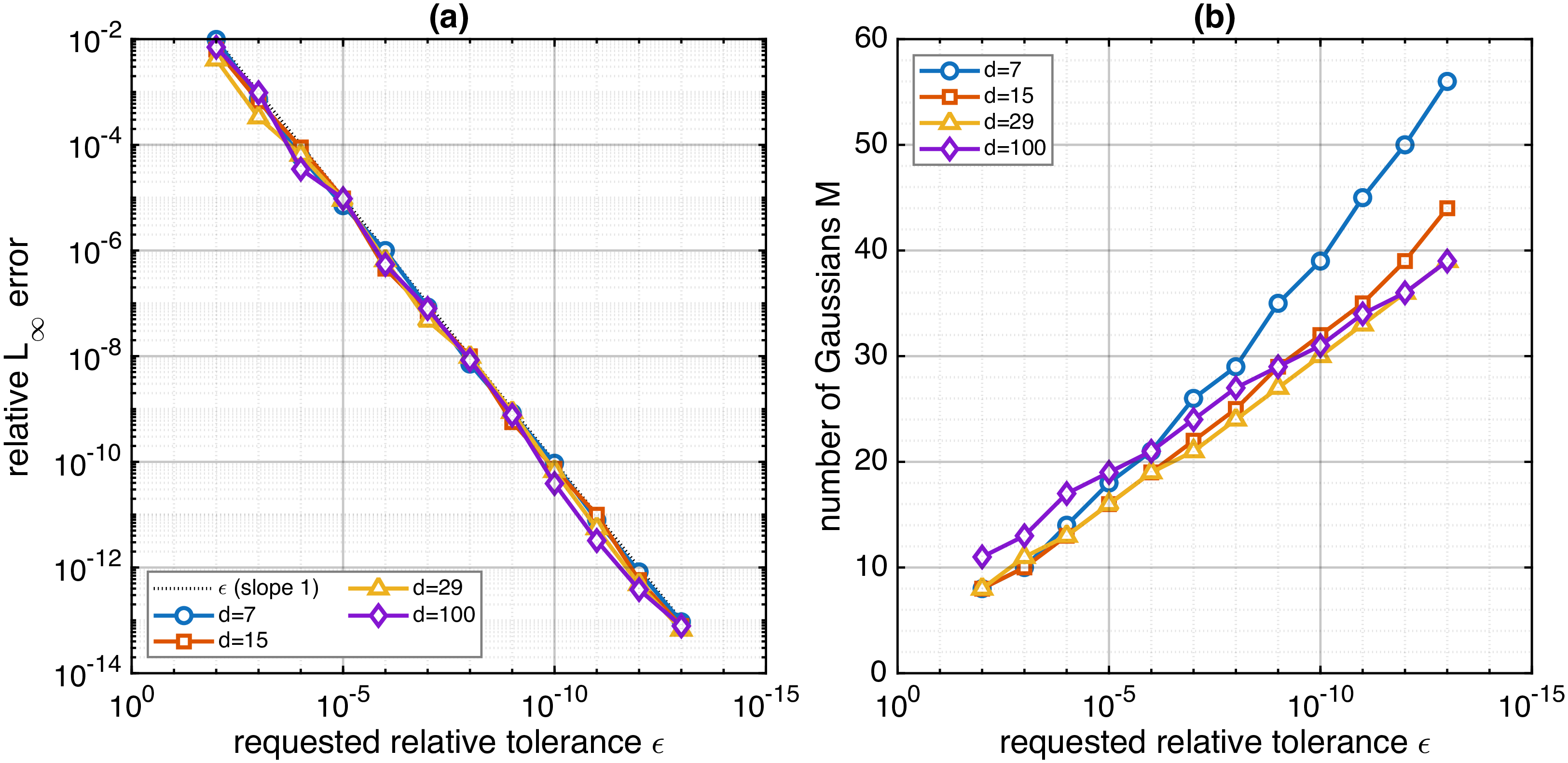
We first verify that the SOG solver attains a prescribed accuracy in moderate and high dimension. Fixing \(D_f=1\), \(D_o=0\), \(\alpha=1/2\), and \(T=1\), we prescribe a relative accuracy \(\epsilon\), select the SOG parameters by 1 (with the step \(h\) initialized by 45 and the band by 47 49 ), and measure the relative \(L_\infty\) error of \(p_{\text{SOG}}\) against the exact Cauchy density 51 over \(y\in[0,2]\). The dimensions in 3 are \(d=7,15,29,100\). Panel (a) shows that the measured error tracks the prescribed tolerance with slope one across eleven orders of magnitude, reaching \(7.8\times10^{-14}\) at \(d=100\) when \(\epsilon=10^{-13}\). The accuracy is therefore limited by the prescribed tolerance and, ultimately, by the arithmetic of the double-precision evaluation. Two further observations confirm the solution-level parameter selection of 3.4:
The number of Gaussians \(M\) grows only logarithmically in \(1/\epsilon\) (3 (b)). Across all dimensions and tolerances shown, \(M\) lies between \(8\) and \(56\); at \(\epsilon=10^{-13}\) the term counts are \(56,44,39,39\) for \(d=7,15,29,100\), respectively. The dimension enters through both the step \(h\propto(d+1)^{-1/2}\) (asymptotically, 46 ) and the truncation band 47 49 . The decrease over this range is the low-to-moderate-dimensional branch of the non-monotonic dependence described in Remark [rmk::nexp95d]; in very high dimension the displacement-band term \(\ln(1+\eta_{\max}^2)/h\propto\sqrt d\) dominates and \(M\) grows again (4.4).
Replacing the evaluation of \(\rho_\alpha\) by the exact closed form of the one-sided stable (Lévy) density \(\rho_{1/2}(s)=\tfrac{1}{2\sqrt{\pi}} s^{-3/2}e^{-1/(4s)}\) reproduces the errors of 3 to every displayed digit. The density evaluation therefore does not limit the accuracy; the residual error is due entirely to the SOE truncation.
For \(\alpha=1/2\), Proposition [prop::disc] controls the relative discretization error independently of the evaluation point and of \(T\), and 1 enforces \(E_{\mathcal{A}}\le\epsilon\) for the finite retained band on the prescribed spatial window; by Proposition [prop::Q95sog], this scaled relative error equals that of the physical Green’s function, so the guarantee transfers directly to \(p_{\text{SOG}}\) and the measured error tracks \(\epsilon\) uniformly in \(d\).
The experiments reported here use \(\alpha\in[0.1,0.9]\). As \(\alpha\to0^+\) or \(\alpha\to1^-\) the bound on \(I_\alpha\) in Theorem 2 diverges, so the trapezoidal step \(h\) shrinks and the term count \(M\) grows rapidly; this is intrinsic, since the representing density becomes singular at both endpoints, degenerating to a Dirac measure at \(z=1\) as \(\alpha\to1^-\) and to a nonregular limiting object as \(\alpha\to0^+\). Independently, direct evaluation of \(\rho_\alpha\) becomes ill-conditioned near the endpoints: in our implementation, the relative error of the Laplace identity \(\int_0^\infty\rho_\alpha(t)e^{-xt}\mathrm{d}t=e^{-x^\alpha}\) exceeds \(10^{-3}\) for \(\alpha\lesssim0.05\) and \(\alpha\gtrsim0.99\), while it is at the level of machine precision throughout \(\alpha\in[0.1,0.95]\). Accurate computation in the immediate vicinity of the endpoints requires a dedicated evaluator for \(\rho_\alpha\) (for instance, numerical steepest descent on the contour of Appendix 6) and is left to future work.
4.2 Self-convergence study↩︎
The exact Cauchy reference 51 is available only for \(\alpha=1/2\). For other fractional orders we assess the assembled solution by self-convergence: the chosen finite Gaussian sum is compared, on the scaled radial interval, with a refined reference at half the step and a wider band. Since the inverse Fourier transform of each Gaussian is exact, this probes the only numerical approximation in the method, the SOE approximation of \(e^{-x^\alpha}\) on the active solution window. These entries should therefore be interpreted as finite-domain self-convergence estimates; the independent exact-reference checks are the \(\alpha=1/2\) row and the Cauchy tests in the other tables.
| \(\alpha\) | \(\eta_{\max}\) | \(M\) | \(h\) | error |
|---|---|---|---|---|
| 0.1 | \(5.96\,\textrm{e}{2}\) | 2492 | \(3.43\,\textrm{e}{-2}\) | \(4.5\,\textrm{e}{-12}\) |
| 0.3 | \(1.34\,\textrm{e}{1}\) | 631 | \(2.67\,\textrm{e}{-2}\) | \(1.5\,\textrm{e}{-11}\) |
| 0.5 | \(6.25\,\textrm{e}{0}\) | 126 | \(3.43\,\textrm{e}{-2}\) | \(9.1\,\textrm{e}{-13}\) |
| 0.7 | \(4.51\,\textrm{e}{0}\) | 25 | \(2.08\,\textrm{e}{-2}\) | \(1.2\,\textrm{e}{-11}\) |
| 0.9 | \(3.77\,\textrm{e}{0}\) | 21 | \(9.89\,\textrm{e}{-3}\) | \(6.5\,\textrm{e}{-12}\) |
1 reports the result at \(d=1000\) for \(\alpha=0.1,0.3,0.5,0.7,0.9\), with \(D_o=0\), \(D_f=8\), \(t=0.04\), and \(y\in[0,2]\), at prescribed tolerance \(\epsilon=10^{-10}\). It also lists the scaled endpoint \(\eta_{\max}=R/(D_ft)^{1/(2\alpha)}\), since this – not \(t\) alone – sets the active range of Gaussian scales. The largest term count occurs at \(\alpha=0.1\), where the fixed window maps to the largest scaled radius; the \(\alpha=0.3\) row, in which a saddle-point approximation of \(\rho_\alpha\) is blended smoothly with the direct evaluation at small \(s\), indicates that the density evaluation is not the limiting factor in this test. The \(\alpha=1/2\) row, where the true error against 51 is available, also meets the tolerance and anchors the self-convergence estimates at the other orders.
4.3 Robustness across time and dimension↩︎
We now fix a relative tolerance \(\epsilon=10^{-12}\) and, for each \((t,d)\), select the SOG parameters from 1 (with the \(\alpha=1/2\) step from 45 and band from 47 49 ). We evaluate \(p_{\text{SOG}}\) for \(D_o=0\), \(D_f=8\), \(\alpha=1/2\) on the higher-dimensional part of the \(t\times d\) grid used in [19], reporting the maximum relative error over \(y\in[0,2]\).
| \(d\) | 5 | 9 | 13 | 17 | 21 | 25 | 29 |
|---|---|---|---|---|---|---|---|
| SOG (tested \(t\) grid) | 1.0 e-12 | 1.0 e-12 | 1.0 e-12 | 1.0 e-12 | 1.0 e-12 | 1.0 e-12 | 1.0 e-12 |
| [19], \(t{=}0.004\) | 2.2 e-9 | 2.2 e-6 | 3.2 e-3 | 1.7 e+0 | 5.4 e+2 | 2.3 e+6 | 3.1 e+9 |
| [19], \(t{=}0.2\) | 7.7 e-16 | 9.6 e-16 | 1.7 e-15 | 1.9 e-15 | 2.8 e-15 | 5.5 e-15 | 7.1 e-15 |
![Figure 4: Maximum relative error versus dimension for the pure-fractional case (D_o=0, D_f=8, \alpha=1/2). The three SOG curves for t=0.004,0.04,0.2 coincide and stay at the prescribed tolerance \epsilon=10^{-12} (dotted), confirming that the approximation determined by \eta_{\max} is reused across the time grid and remains uniform in d. For comparison, the integral-quadrature solver of [19] at t=0.004 (red) loses accuracy rapidly as d grows, reaching \mathcal{O}(10^{9}) at d=29 on this test.](/article/2606.28184/fig_robustness.png "fig:")
Two features stand out. First, the time dependence is handled by self-similar scaling (Proposition [prop::disc] and Remark [rmk::selfsim]): a single approximation sized at \(t_{\min}=0.004\), using \(M=71\)–\(82\) terms over \(d=5\)–\(29\), holds relative error about \(10^{-12}\) across the whole time grid, with no degradation as \(t\to0^+\) (the regime in which the solution concentrates toward the Dirac measure). Second, the error is uniform in dimension, staying at the prescribed \(10^{-12}\) throughout. 2 contrasts this with the integral solver of [19]: at small time (\(t=0.004\)) its relative error grows rapidly over the tested dimensions, exceeding unity for \(d\ge17\) and reaching \(\mathcal{O}(10^{9})\) at \(d=29\), whereas at moderate time (\(t=0.2\)) it attains machine precision. The two approaches are thus complementary: the integral solver of [19] is effective for high-precision evaluation in low to moderate dimension, while the SOG holds the prescribed accuracy uniformly across the tested \((t,d)\) range – including the small-\(t\), high-\(d\) corner where the integral solver loses accuracy, as shown in 4 – and scales to much higher dimensions (4.4).
4.4 Scaling to very high dimension↩︎
Unlike the oscillatory radial integrand \(r^{d/2}J_{(d-2)/2}(yr)\) that limits [19] to moderate \(d\), the SOG solution is a positive sum of separable Gaussians, so its logarithm can be evaluated stably. Setting \(a_\ell(\boldsymbol{x})=\log w_\ell-\tfrac{d}{2}\log(4\pi C_\ell^{T}) -|\boldsymbol{x}-\boldsymbol{x}_0^T|^2/(4C_\ell^{T})\) and \(a_\star=\max_\ell a_\ell(\boldsymbol{x})\), \[\label{eq::logsumexp} \log p_{\text{SOG}}(\boldsymbol{x},T)=a_\star+\log\sum_{\ell} \exp\!\big(a_\ell(\boldsymbol{x})-a_\star\big),\tag{52}\] so that the per-term magnitudes \((4\pi C_\ell^{T})^{-d/2}\), which overflow or underflow for large \(d\), never appear explicitly. Each evaluation requires \(O(M)\) operations for the radial profile.
| \(d\) | \(100\) | \(1{,}000\) | \(10{,}000\) | \(100{,}000\) |
|---|---|---|---|---|
| terms \(M\) | \(36\) | \(63\) | \(156\) | \(451\) |
| relative error | \(9.9\,\textrm{e}{-13}\) | \(1.6\,\textrm{e}{-12}\) | \(7.3\,\textrm{e}{-12}\) | \(5.8\,\textrm{e}{-11}\) |
| time per point (μs) | \(0.33\) | \(0.48\) | \(0.96\) | \(4.2\) |
These dimensions exceed those reached in the radial-quadrature experiments of [19]. We again use the exact Cauchy solution 51 : although its magnitude over- or underflows, its logarithm is computable to full relative precision in any dimension via the log-Gamma function. 3 reports the relative error and evaluation time per point for \(d\) up to \(10^{5}\). The SOG attains ten-digit relative accuracy at \(d=10^{5}\) in about \(4\) μs per point, with the term count \(M\) rising only from \(36\) at \(d=100\) to \(451\) at \(d=10^5\) (the slow large-\(d\) growth is analyzed in Remark [rmk::nexp95d]). These tests give deterministic, high-accuracy evaluations at dimensions beyond the reach of radial-quadrature methods.
4.5 General initial data: tensor-product representations↩︎
A key advantage of the SOG representation is that it provides a reusable building block that maps separated (tensor-product) data to separated data. The SOG approximation \(p_{\text{SOG}}\) is itself a rank-\(M\) separated function: by 22 each term \(p_\ell\) is a tensor product \(\prod_{j=1}^{d} g_\ell(x_j)\) of one-dimensional Gaussians. Consequently, for any initial datum written as a linear combination of tensor products, \[\label{eq::tensor95ic} p(\boldsymbol{x},0)=\sum_{r=1}^{R}\prod_{j=1}^{d}\phi_{r,j}(x_j),\tag{53}\] linearity and the separability of the heat kernel give the solution in closed form as \[\label{eq::tensor95sol} p(\boldsymbol{x},T)=\sum_{r=1}^{R}\sum_{\ell=-M_1}^{M_2}w_\ell\prod_{j=1}^{d} \big(g_\ell * \phi_{r,j}\big)(x_j-b_jT),\tag{54}\] which is again a sum of tensor products. The dimension \(d\) enters only through the one-dimensional convolutions \(g_\ell*\phi_{r,j}\), and the rank grows from \(R\) to \(RM\), recompressible by standard tensor-rank truncation. Such separated, low-rank formats – the canonical, Tucker, and tensor-train decompositions [21]–[23], [39], [40] and the related tensor networks [41]–[43] – provide a natural high-dimensional function class for this solver. Tensor neural networks [26]–[28], [44] can be used to construct separated approximations for more general initial data.
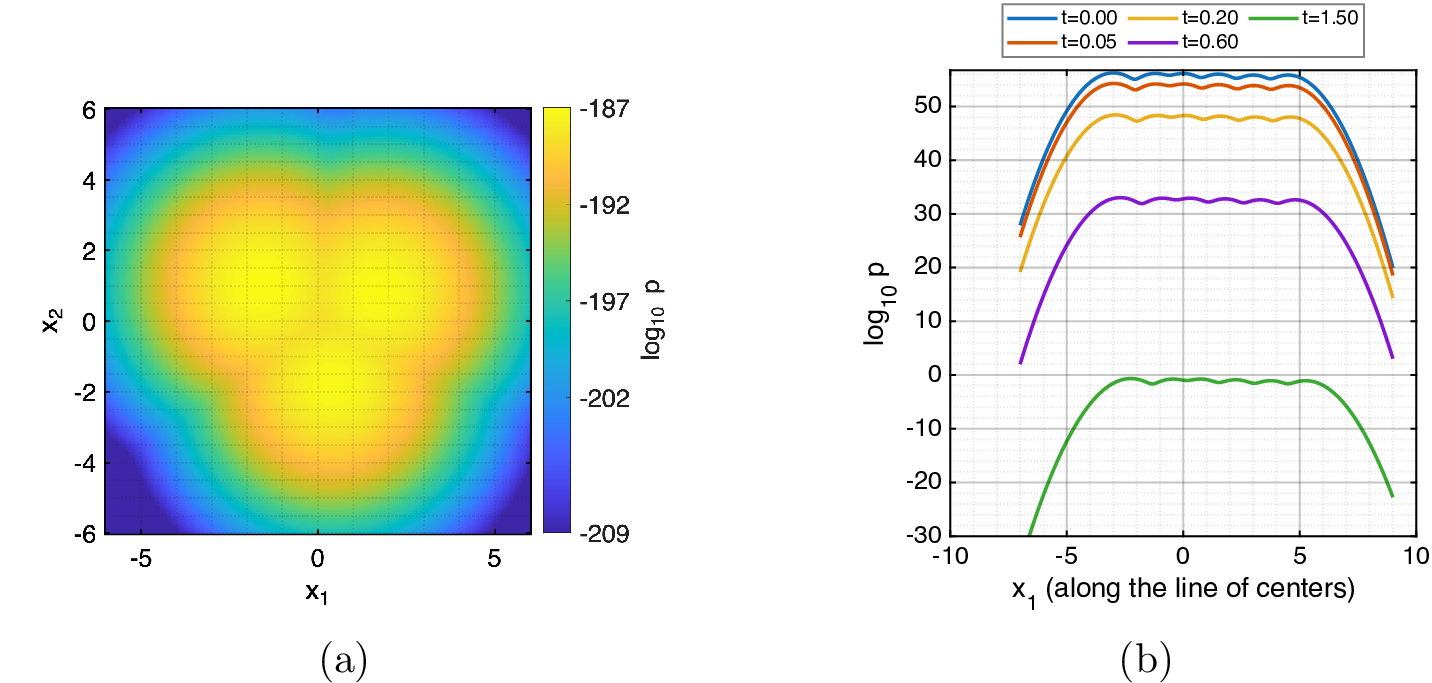
Gaussian initial data are the canonical example: the one-dimensional convolutions remain Gaussian and are available analytically. Since each \(p_\ell\) in 22 has covariance \(2C_\ell^{T}I\), the solution for the initial condition \[p(\boldsymbol{x},0)=\sum_{j=1}^{N_g}a_j\, \mathcal{N}(\boldsymbol{x};\boldsymbol{c}_j,\sigma_j^2 I)\] is \[\label{eq::sog95ic} p(\boldsymbol{x},T)=\sum_{j=1}^{N_g}\sum_{\ell=-M_1}^{M_2}a_j\,w_\ell\, \mathcal{N}\!\big(\boldsymbol{x};\,\boldsymbol{c}_j+\boldsymbol{b}T,\,(\sigma_j^2+2C_\ell^{T})I\big),\tag{55}\] a sum of \(N_gM\) Gaussians, each a tensor product across the \(d\) coordinates, stored and manipulated in the same factored \(O(MdN)\) representation as the fundamental solution.
We test 55 directly in high dimension. For a single Gaussian source, the value at the advected center has the independent non-oscillatory reference \[\frac{\Omega_d}{(2\pi)^d}\int_0^\infty r^{d-1}\exp\!\left(-\frac{\sigma^2r^2}{2}-D_fT r^{2\alpha}\right)\mathrm{d}r,\] which is evaluated after a saddle-point change of variables and does not involve the oscillatory Bessel integral. With \(\alpha=1/2\), \(\sigma=0.5\), \(D_f=1\), and a broad \(M=3251\) term SOE that preserves \(\sum_\ell w_\ell=1\) to the displayed digits, the relative errors at \(T=0.1\) are \(1.1\times10^{-13}\), \(2.7\times10^{-12}\), and \(6.2\times10^{-11}\) for \(d=10^3,10^4,10^5\), respectively; at \(T=1\) they are \(3.4\times10^{-13}\), \(9.1\times10^{-13}\), and \(9.8\times10^{-11}\).
5 (a) shows a two-dimensional slice of the \(d=1000\) solution for a non-radial, three-Gaussian initial condition under drift and pure fractional diffusion, computed from the separated representation directly rather than by reducing the data to a radial profile.
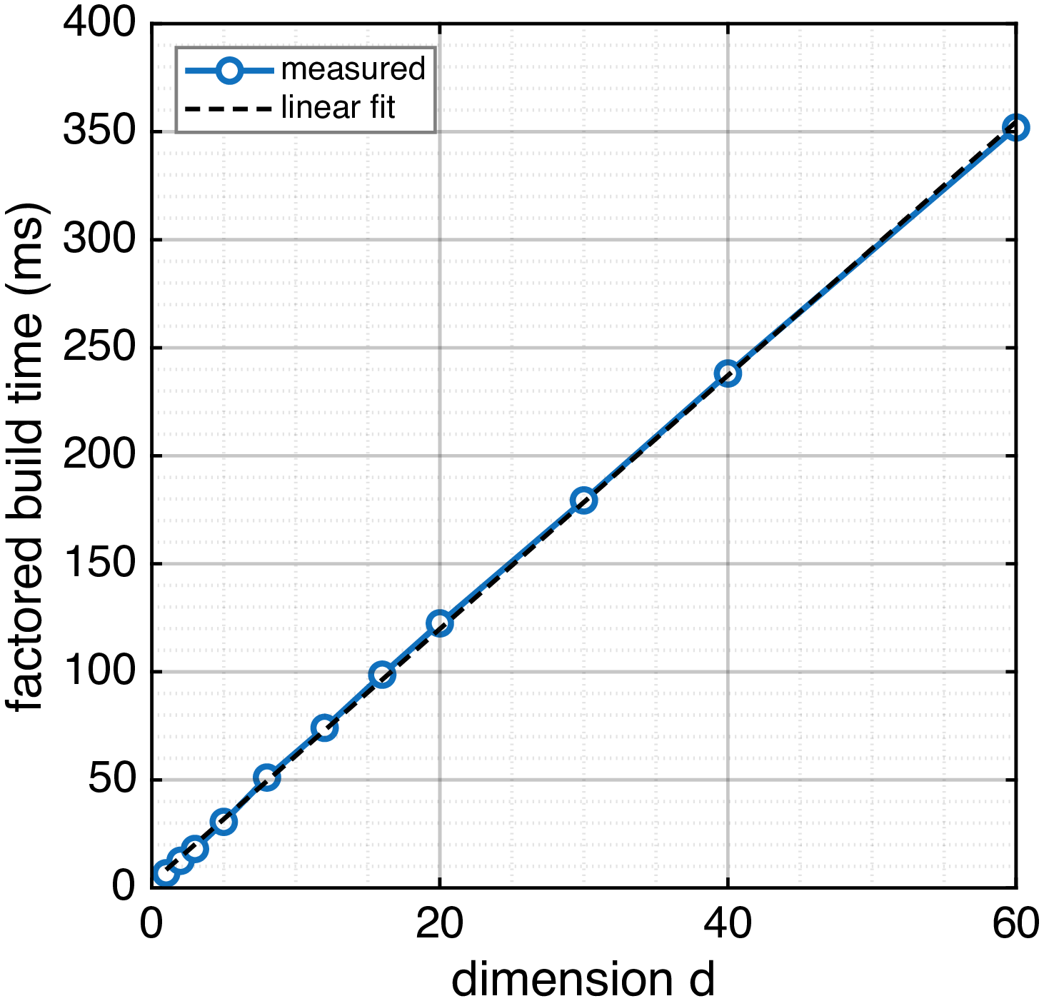
Finally, 6 confirms the linear-in-\(d\) cost. Holding the SOG approximation fixed at \(M=1012\) terms (\(P=N_gM=8096\) Gaussians for \(N_g=8\) sources) and varying only the dimension, the factored assembly time is indistinguishable from a straight line through the origin, reaching \(0.38\) s at \(d=60\). In \(d=10\) the same \(P=8096\) factored Gaussians are assembled in \(0.07\) s, and a factored evaluation agrees with the explicit double sum over \(j\) and \(\ell\) to \(8\times10^{-16}\) – whereas the corresponding dense tensor has \(N^{10}\approx10^{18}\) entries and is not a feasible object to store.
Combining this building block with the logarithmic evaluation of 4.4 lets us evolve sum-of-Gaussians initial data in very high dimension; 5 (b) shows a six-Gaussian initial condition evolved in \(d=1000\) with drift along the line of centers. Spanning more than eighty orders of magnitude, the solution is representable only through its logarithm 52 . The mass \(\int_{\mathbb{R}^d}p\,\mathrm{d}\boldsymbol{x} =\big(\sum_j a_j\big)\big(\sum_\ell w_\ell\big)\) is conserved to \(1.000000\) at every time, in any dimension, and evaluating one 600-point time slice costs about \(0.09\) s at \(d=1000\).
5 Conclusion↩︎
We have developed a sum-of-Gaussians solver for the high-dimensional fractional Fokker–Planck equation with high-order accuracy and error control. The construction uses the complete monotonicity of the fractional symbol \(e^{-D_ft|\boldsymbol{k}|^{2\alpha}}\), which represents it as a continuous superposition of Gaussians. Discretizing that superposition gives a finite sum of ordinary heat flows that act independently in each coordinate, with storage and assembly cost linear in the dimension and quadrature parameters fixed a priori for any target accuracy. In our experiments the solver attains more than ten digits of accuracy, with \(M\) growing only logarithmically as the tolerance tightens and the accuracy uniform across the time windows tested; evaluating the positive Gaussian form through its logarithm carries the computation to dimension \(10^{5}\).
Because the method approximates the fundamental solution by a separated sum of Gaussians, it propagates any tensor-product initial datum in closed form, so the only additional ingredient needed for more general data is a separated, low-rank representation of it. Sparse-grid and tensor neural network approximation frameworks are compatible with this requirement and can be combined directly with the present solver. When a high-dimensional Fourier symbol or interaction kernel admits an accurate Gaussian-sum expansion, the expansion expresses nonseparable terms as sums of separable Gaussian contributions. The FFPE results presented here therefore support the use of SOG approximations as building blocks for separable representations of kernels and solution operators in high-dimensional PDEs.
The approach is also relevant beyond the particular FFPE fundamental solution studied here. For a linear constant-coefficient evolution equation in high dimension, if the Fourier-space propagator admits an accurate Gaussian-sum approximation, the same construction expresses the solution operator as a sum of separable Gaussian evolution operators. For many nonlinear evolution equations, applying an unconditionally energy-stable scalar auxiliary variable (SAV) temporal discretization reduces each time step to a linear problem with known source terms [33]. When this linear problem has a constant-coefficient solution operator that admits an accurate and efficient Gaussian-sum representation, the present solver can serve as a building block for high-dimensional nonlinear evolution PDEs.
Acknowledgments↩︎
The Flatiron Institute is a division of the Simons Foundation. The work of Q. Zhou was supported by the National Natural Science Foundation of China (Grant No. 125B2023).
6 A bound for \(|\rho_\alpha(z)|\) on \(|z|\le 1\)↩︎
In this section, we provide some estimates on \(|\rho_\alpha(z)|\), where \(\rho_\alpha(z)\) is the one-sided stable PDF with \(0<\alpha<1\), analytically continued to the complex plane. Denote \(z=re^{i\theta}\), where the modulus \(r\in [0,1]\) and the angle \(|\theta|<\theta_{*}(1-\alpha)\), with \(0<\theta_{*}<\pi/6\) a critical angle to be determined later. The inverse Laplace transform gives \[\label{eq::ILT} \rho_\alpha(z)=\frac{1}{2\pi i}\int_{C}e^{\Phi_{z}(s)}\mathrm{d}s,\tag{56}\] where \[\label{eq::phase95original} \Phi_{z}(s)=sz-s^{\alpha},\tag{57}\] and \(C\) is an appropriate inversion contour. To estimate \(|\rho_\alpha(z)|\), we proceed in the following steps:
Find the saddle point of \(\Phi_z(s)\). Transform \(C\) into the (approximated) steepest descent contour. Specifically, a parabolic contour derived from the local and global properties of \(\Phi_z(s)\).
Analyze properties of the phase function on the parabolic contour.
Based on the results above, provide an upper bound of \(|\rho_\alpha(z)|\).
We proceed according to these steps in sequence.
6.1 The parabolic contour↩︎
From 57 , we take derivative of \(\Phi_z(s)\), then \[\label{eq::Phi95deri} \Phi_z'(s)=z-\alpha s^{\alpha-1},\tag{58}\] which shows the saddle point is \(s_c=(\alpha/z)^{1/(1-\alpha)}\). The polar representation of \(s_c\) is provided by \(s_c=\sigma e^{i\psi_0}\), where \[\label{eq::sigma95psi} \sigma=\alpha^{1/(1-\alpha)}r^{-1/(1-\alpha)},\quad \psi_0=-\frac{\theta}{1-\alpha}.\tag{59}\] Thus one has \(\Phi_z(s_c)=-(1-\alpha)s_c^{\alpha}\) and \(\Phi_z''(s_c)=\lambda s_c^{\alpha-2}\), \(\lambda=\alpha(1-\alpha)\). Based on these results, one selects the parameterized contour as \(s(u)=s_cw(u)\), where \[\label{eq::sd95quad} w(u)=1+iu-\eta u^2,\quad \eta=\frac{2-\alpha}{6}\in(\frac{1}{6},\frac{1}{3}),\quad u\in\mathbb{R}.\tag{60}\] Correspondingly, the phase and the parameter derivative have the expression as \[\label{eq::phase95para} \Phi_z(s(u))=\sigma^\alpha e^{i\phi} (\alpha w(u) - w(u)^\alpha), \quad s'(u)=\sigma e^{i\psi_0}(i-2\eta u).\tag{61}\] where \(\phi=\alpha\psi_0\). Hence the integral in 56 becomes \[\label{eq::integral95transform} \rho_\alpha(z)=\frac{1}{2\pi i}\int_{-\infty}^{\infty} \exp\Big(\sigma^\alpha e^{i\phi}(\alpha w(u) - w(u)^\alpha)\Big) e^{i\psi_0}\sigma\bigl(i-2\eta u\bigr)\mathrm{d}u.\tag{62}\] Define the main phase function as \[\label{eq::main95phase} F(u):=\operatorname{Re}\{e^{i\phi}(\alpha w(u)-w(u)^{\alpha})\},\tag{63}\] and one readily derives the upper bound \[\label{eq::rho95bound} |\rho_\alpha(z)|\le\frac{1}{2\pi}\int_{-\infty}^{\infty} \exp\Big(\sigma^\alpha F(u)\Big)\cdot \sigma(1+2\eta |u|)\mathrm{d}u.\tag{64}\]
6.2 The global maximum property of \(F(u)\)↩︎
For the main phase function \(F(u)\) defined in 63 , Proposition [prop::global95maximum] characterizes its most essential property.
Under suitable restrictions on the contour angle \(\theta\), the main phase function \(F(u)\) is monotonic on both sides of \(u=0\), and \(F(0)\) is its unique maximum. That is, \(F'(u)>0\) for all \(u<0\), and \(F'(u)<0\) for all \(u>0\).
By the symmetry \(F(-u;\phi)=F(u;-\phi)\), it suffices to prove \(F'(u)<0\) for \(u>0\) and all admissible \(\phi\). The case \(u<0\) then follows by replacing \(\phi\) with \(-\phi\). Before proving the global maximum property, we first consider the behavior of \(F(u)\) as \(|u|\rightarrow0\) and \(|u|\rightarrow \infty\), described in Lemmas 5 and 6.
Lemma 5 (Small-\(|u|\) Gaussian control). \[F(u)=-(1-\alpha)\cos\phi-\frac{\lambda}{2}\cos\phi u^2+O(u^4)\quad (|u|\to 0).\] Hence \(u=0\) is a strict local maximizer of \(F(u)\).
Proof. Let \(G(u):=\alpha w(u)-w(u)^\alpha\). On the principal branch, we have \[G(0)=-(1-\alpha),\quad G'(0)=0,\quad G''(0)=-\lambda,\quad G^{(3)}(0)=0.\] The result follows from the Taylor expansion. ◻
Lemma 6 (Large-\(|u|\) quadratic dominance). For sufficiently large \(|u|\), \[F(u)\le-\frac{\alpha \eta}{2}\cos\phi\cdot u^2.\]
Proof. This simply follows from the facts that \(0<\alpha<1\), \(\alpha w(u)\) dominates \(w(u)^\alpha\) for large \(|u|\), and \(-\eta u^2\) dominates in \(w(u)\) for large \(|u|\). ◻
Now we introduce the polar representation \(w(u):=\varrho(u)e^{i\delta(u)}\), with \(\varrho(u)=|w(u)|\) and \(\delta(u)=\arg w(u)\in (0,\pi)\). Lemma 7 shows that the argument of \(w(u)\) is monotonically increasing for \(u>0\).
Lemma 7 (Argument of \(w(u)\) is increasing). \[\delta'(u)=\frac{1+\eta u^2}{(1-\eta u^2)^2+u^2}>0, \quad\forall u>0,\] and \[\delta\!\left(\frac{1}{\sqrt \eta}\right)=\frac{\pi}{2}.\]
Proof. Choose the continuous branch of \(\log\) along the path \(u\mapsto w(u)\) and note \(\delta(u)=\mathrm{Im}\log w(u)\). Then \[\delta'(u)=\mathrm{Im}\left(\frac{w'(u)}{w(u)}\right) =\mathrm{Im}\left(\frac{i-2\eta u}{1+i u-\eta u^2}\right) =\frac{1+\eta u^2}{(1-\eta u^2)^2+u^2}>0,\] after multiplying numerator and denominator by \(\overline{w(u)}\) and taking imaginary parts.
For the stated value at \(u=1/\sqrt \eta\), \[w\left(\frac{1}{\sqrt \eta}\right)=1+i\frac{1}{\sqrt \eta}-\eta\cdot\frac{1}{\eta} = i\frac{1}{\sqrt \eta},\] which is purely imaginary with positive imaginary part. Hence \[\delta(1/\sqrt \eta)=\arg\big(i/\sqrt \eta\big)=\pi/2.\] ◻
Furthermore, with the polar representation of \(w(u)\), the derivative of \(F(u)\) is then \[\label{eq::F95derivative} F'(u)=\operatorname{Re}\Big\{\alpha e^{i\phi}(1-w(u)^{\alpha})w'(u)\Big\}.\tag{65}\] Hence we denote \[\label{eq::tangent} k(u)=2\eta u>0,\quad \tau(u)=\arctan(k(u))\in[0,\frac{\pi}{2}),\quad S(u)=\phi+\tau(u)\tag{66}\] as the positive tangent slope, tangent angle, and the transport angle of \(w'(u)\), respectively, since \(w'(u)=i-2\eta u\). We also introduce auxiliary exponents of modulus and argument that \[\label{eq::auxiliary} \mu(u)=\varrho(u)^{\alpha-1},\quad \beta(u)=(1-\alpha)\delta(u)\in (0,\pi),\tag{67}\] which indicates that \[\label{eq::F95expression} \frac{F'(u)}{\alpha\sqrt{1+k(u)^2}} =\mu(u)\sin\big(S(u)-\beta(u)\big)-\sin S(u).\tag{68}\] Subsequent proofs concerning monotonicity will rely on the expression provided in 68 , requiring a detailed analysis of the ranges and quantitative relationships of \(\mu(u)\), \(S(u)\), and \(\beta(u)\). Lemma 8 provides the bound of \(\varrho(u)\) and \(\mu(u)\).
Lemma 8 (Basic size bounds for \(\varrho\) and \(\mu\)). With \(\varrho(u)=\sqrt{(1-\eta u^2)^2+u^2}\), one has \[\varrho(u)>1\quad\text{for all }u>0,\quad \mu(u):=\varrho(u)^{\alpha-1}=\varrho(u)^{-(1-\alpha)}\in(0,1).\]
Proof. Since \[\varrho(u)^2=1+(1-2\eta)\,u^2+\eta^2 u^4,\qquad \frac{\mathrm{d}}{\mathrm{d}u}\varrho(u)^2 =2u\bigl(1-2\eta+2\eta^2 u^2\bigr)>0\quad(u>0),\] and \(\varrho(0)=1\), it follows that \(\varrho(u)>1\) for \(u>0\). Hence \(\mu(u)\in(0,1)\). ◻
For the transport angle \(S(u)\), Lemmas 9 and 10 show the geometry of the case when \(S(u)\ge \pi/2\).
Lemma 9 (Geometry at \(S=\pi/2\)). Assume that \[\label{eq::phi95assume} 0<\phi=\alpha\psi_0=-\frac{\alpha\theta}{1-\alpha}\le \alpha\theta_*.\qquad{(9)}\] Then there exists a unique \(u_0>0\) with \(S(u_0)=\pi/2\), characterized by \[2\eta u_0=\cot\phi.\] Furthermore, under the standing constraints \(\eta\in(1/6,1/3)\) and \(|\phi|\le \pi\alpha/6\), one has \[u_0\ge\frac{1}{\sqrt \eta},\quad \delta(u)\ge\frac{\pi}{2},\quad\forall u\ge u_0.\]
Proof. Since \(0<\phi\le \pi/6\), one has \(\tan\phi\le \tan(\pi/6)=1/\sqrt3\). Note that \(\eta\le 1/3\), one has \[\frac{1}{\sqrt3}\;\le\;\frac{1}{2\sqrt \eta}\quad\Longrightarrow\quad \tan\phi\le \frac{1}{2\sqrt \eta}\quad\Longrightarrow\quad \cot\phi\ge 2\sqrt \eta.\] Therefore, \[\label{eq::u095estimate} u_0=\frac{\cot\phi}{2\eta}\ge \frac{2\sqrt \eta}{2\eta}=\frac{1}{\sqrt \eta}.\tag{69}\] By Lemma 7, \(\delta\) is increasing and \(\delta(1/\sqrt \eta)=\pi/2\), so \(\delta(u)\ge \pi/2\) for \(u\ge u_0\). ◻
Lemma 10 (Second quadrant when \(S(u)>\pi/2\)). If \(u>0\) and \(S(u)>\pi/2\), then \(w(u)=1+iu-\eta u^2\) lies in the second quadrant. In particular, \[\delta(u) \in\;\Big(\frac{\pi}{2},\pi\Big),\]
Proof. Since \(S(u)=\phi+\tau(u)\) with \(\tau(u)=\arctan k(u)\) strictly increasing in \(k\), the condition \(S(u)>\pi/2\) is equivalent to \[\tau(u)>\frac{\pi}{2}-\phi \quad\Longleftrightarrow\quad k(u)>\cot\phi.\] Because \(S(u)>\pi/2\) forces \(\phi>0\) with \(0<\phi\le \pi/6\), one has \(\cot\phi\ge\sqrt{3}\). Using \(\eta\le1/3\), one gets \(\sqrt{3}\ge 2\sqrt \eta\), hence \[k(u)>\cot\phi\;\ge\;2\sqrt \eta \quad\Longrightarrow\quad u>1/\sqrt \eta.\] Since \[w(u)=(1-\eta u^2)+iu,\] one has \(1-\eta u^2<0\) while \(u>1/\sqrt \eta\). Thus \(\operatorname{Re}\{w(u)\}<0\) and \(\operatorname{Im}\{w(u)\}>0\), so \(w(u)\) lies in the second quadrant and therefore \(\delta(u)\in(\pi/2,\pi)\). ◻
Based on all the properties discussed above, we refine the angular constraints of Proposition [prop::global95maximum] and provide a proof that \(F(u)\) has a unique global maximum at \(F(0)\). The detailed description is given in Theorem 3.
Theorem 3 (Strict monotonicity of the main phase \(F(u)\)). Let \(c_{\star}=1/9\) and \(\theta_{\star}=\arctan c_{\star}\). Suppose that \(|\theta|\le \theta_{\star}(1-\alpha)\) and thus \(|\phi|\le \alpha\theta_{\star}\). For \(u>0\), \[F'(u)<0.\] Consequently \(F\) is strictly decreasing on \((0,\infty)\), strictly increasing on \((-\infty,0)\), and attains its unique global maximum at \(u=0\).
Proving Theorem 3 requires a detailed discussion of the phase relationship between the two angles \(S(u)\) and \(\beta(u)\). Recall that \(S(u)=\phi+\tau(u)\in[-\theta_{*},\pi/2+\theta_{*})\) and \(\beta(u)=(1-\alpha)\delta(u)\in (0,\pi)\). For convenience, we split the whole phase diagram into four parts, which is clearly shown in 7. Specifically, the four cases are:
Case A. \(S(u)< 0\).
Case B. \(0\le S(u)\le \pi/2\).
Case C. \(S(u)>\pi/2\), and \(\beta(u)\ge\pi/2\).
Case D. \(S(u)>\pi/2\), and \(0<\beta(u)<\pi/2\).
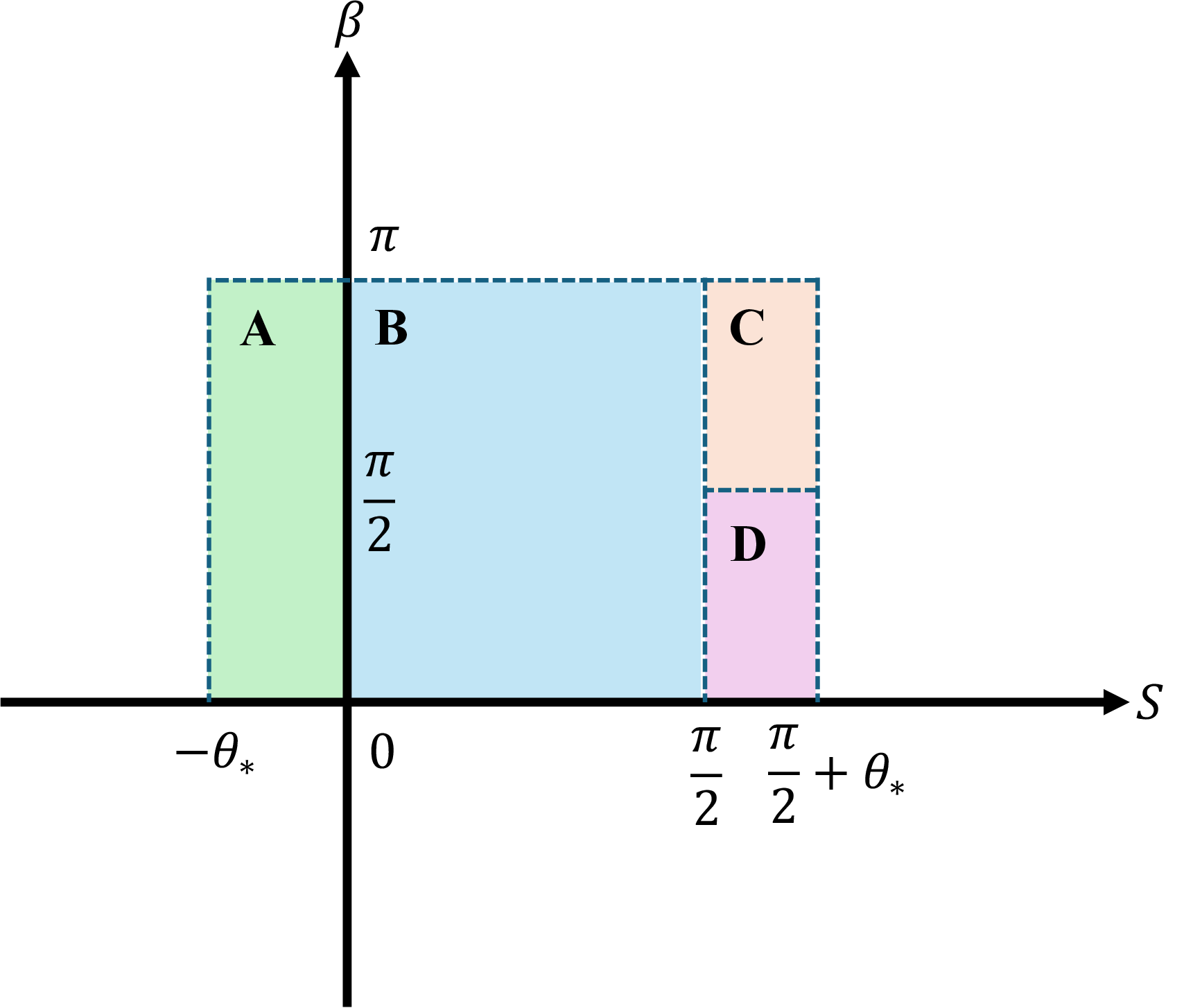
The following Propositions [prop::A]-[prop::D] provide the whole proof process of Theorem 3.
If \(S(u)<0\), then \(F'(u)<0\).
Proof. Since \(S(u)=\phi+\tau(u)<0\) and \(\tau(u)=\arctan(2\eta u)>0\), one must have \(\phi<0\). Since \(\tau(u)\) and \(S(u)\) are strictly increasing, we denote the critical value \[u_{*}=\tan(-\phi)/(2\eta)>0\] such that \(S(u_{*})=0\), so that Case A corresponds to \(u\in [0,u_{*})\). Let \(\zeta(u)=|\tan S(u)|=-\tan S(u)\), then one has the bound that \[\label{eq::bound95tu} 0\le \zeta(u)\le \tan(-\phi)\le \tan(\alpha\theta_{*})\le c_{*}=1/9,\tag{70}\] which also implies that \[\label{eq::bound95u42} 0<u_{*}\le c_{*}/(2\eta)<1/3\tag{71}\] since \(\eta\in (1/6,1/3)\). Rewrite 68 as the form of \[\frac{F'(u)}{\alpha\sqrt{1+k(u)^2}}=-\cos S(u)J(u),\] where \[\label{eq::J} J(u)=\mu(u)\sin\beta(u)-(1-\mu(u)\cos\beta(u))\zeta(u),\tag{72}\] and it suffices to show \(J(u)>0\) for \(u\in(0,1/3)\).
Recall that \(w(u)=(1-\eta u^2)+iu\), so on the negative-\(S(u)\) interval \(u\in(0,1/3)\) one has \(1/2\le \operatorname{Re}\{w(u)\}\le 1\), which gives \[\label{eq::estimate95cos95delta} \cos \delta(u)=\frac{\operatorname{Re}\{w(u)\}}{\sqrt{\operatorname{Re}\{w(u)\}^2+u^2}}\ge \frac{1}{\sqrt{1+4u^2}}\tag{73}\] with \[\label{eq::estimate95rho} \varrho(u)=\frac{\operatorname{Re}\{w(u)\}}{\cos \delta(u)}\le \sqrt{1+4u^2}.\tag{74}\] Hence the exponent \(\mu(u)=\varrho(u)^{-(1-\alpha)}\) has the lower bound that \[\label{eq::estimate95mu} \mu(u)\ge (1+4u^2)^{-(1-\alpha)/2}\ge 1-2(1-\alpha)u^2,\tag{75}\] where the last inequality is Bernoulli’s inequality, valid since the exponent \(-(1-\alpha)/2\) is negative. And for \(\delta(u)\) itself, a simple estimate reads \[\label{eq::estimate95delta} \arctan(u)\le\delta(u)=\arctan\left(\frac{u}{1-\eta u^2}\right)\le \arctan(2u),\tag{76}\] which implies the bound of \(\beta(u)=(1-\alpha)\delta(u)\) that \[\label{eq::estimate95sin95beta} \sin\beta(u)\ge \frac{2(1-\alpha)}{\pi}\arctan u\ge \frac{2(1-\alpha)}{\pi}\frac{u}{1+u^2}.\tag{77}\] and \[\label{eq::estimate95cos95beta} \cos\beta(u)\ge \cos((1-\alpha)\arctan(2u))\ge 1-2(1-\alpha)^2u^2\tag{78}\] with the well-known relation \[\frac{x}{1+x^2}\le \arctan x\le x,\quad x\in\mathbb{R}.\]
Therefore, with the estimate of 75 77 78 , one has that, for \(u\in(0,u_{*})\subset(0,1/3)\), \[\label{eq::estimate95J} \begin{align} J(u) &\ge \big(1-2(1-\alpha)u^2\big)\cdot \frac{2}{\pi}(1-\alpha)\frac{u}{1+u^2} -\big(4(1-\alpha)u^2\big)\cdot c_{*}\\ &=(1-\alpha)u\left[ \frac{2}{\pi(1+u^2)}\big(1-2(1-\alpha)u^2\big)-4u c_{*} \right]\\ &>(1-\alpha)u\left[\frac{2}{\pi}\cdot\frac{9}{10}\cdot\frac{7}{9}-\frac{4}{27}\right]=(1-\alpha)u\left[\frac{7}{5\pi}-\frac{4}{27}\right]>0,\\ \end{align}\tag{79}\] which guarantees \(F'(u)<0\) for all \(u\) for which the \(S\)–\(\beta\) phase diagram lies in Case A. ◻
If \(0\le S(u)\le\pi/2\), then \(F'(u)<0\).
Proof. One rewrites 68 into \[\label{eq::F95caseB} \frac{F'(u)}{\alpha\sqrt{1+k(u)^2}}=(\mu(u)\cos\beta(u)-1)\sin S(u)-\mu(u)\cos S(u)\sin\beta(u).\tag{80}\] Here, at Case B with \(S(u)\in [0,\pi/2]\), one has \(\cos S\ge 0\), \(\sin\beta>0\), \(\cos\beta\le 1\) and \(\mu\in(0,1)\), which imply that \[\label{estimate95caseB} (\mu\cos\beta-1)\sin S\le(1-1)\sin S\le 0,\quad -\mu \cos S\sin \beta< 0.\tag{81}\] Hence \(F'(u)<0\) holds when the \(S\)–\(\beta\) phase diagram lies in Case B. ◻
If \(S(u)>\pi/2\) and \(\beta(u)\ge\pi/2\), then \(F'(u)<0\).
Proof. For this case, one must have \(\phi>0\) by Lemma 10. Note that \(S(u)\le \phi+\pi/2\) with \(\phi\in(0,\pi/6)\), so at Case C, one has \[\label{eq::estimate95difference} -\frac{\pi}{2}<S(u)-\beta(u)\le \frac{\pi}{2}+\phi-\frac{\pi}{2}\le\frac{\pi}{6},\tag{82}\] which indicates \[\label{eq::estimate95sin95diff} \sin(S(u)-\beta(u))\le 1/2\tag{83}\] and also \[\label{eq::estimate95sin95S} \sin S(u)\ge \sin(\frac{\pi}{2}+\phi)=\cos\phi\ge\frac{\sqrt{3}}{2}.\tag{84}\] Substituting 83 84 into 68 , as well as the relation \(\mu\in(0,1)\), one immediately derives \[\label{eq::estimate95caseC} \frac{F'(u)}{\alpha\sqrt{1+k(u)^2}}=\mu\sin(S-\beta)-\sin S\le \frac{1}{2}-\frac{\sqrt{3}}{2}<0.\tag{85}\] ◻
If \(S(u)>\pi/2\) and \(0<\beta(u)< \pi/2\), then \(F'(u)<0\).
Proof. For this case, one must have \(\phi>0\) by Lemma 10. On the strip of \(S(u)\in(\pi/2,\pi/2+\phi]\), one firstly has \[\label{eq::estimate95S95caseD} \sin S\ge\sin\Big(\frac{\pi}{2}+\phi\Big)=\cos\phi, \quad \cos S\ge \cos\Big(\frac{\pi}{2}+\phi\Big)= -\sin\phi.\tag{86}\] For the right-hand-side of 68 , one has \[\label{eq::estimate95F95caseD} \begin{align} \mu\sin(S-\beta)-\sin S&=\sin S(\mu\cos\beta-1)-\mu\cos S\sin \beta\\ &\le \cos \phi(\mu\cos\beta-1)+\mu\sin \phi\sin \beta\\ &= \mu\cos(\beta-\phi)-\cos\phi. \end{align}\tag{87}\] Hence it suffices to show that, for \(u>0\) satisfies \(S(u)\in (\pi/2,\pi/2+\phi]\) and \(\beta\in (0,\pi/2)\), \[\label{eq::relation95caseD} T(u):=\mu(u)\cos(\beta(u)-\phi)<\cos \phi.\tag{88}\] Here we introduce the critical value \(u_0=\cot\phi/(2\eta)\) in Lemma 9 such that \(S(u_0)=\pi/2\), which forces \(u>u_0\). At \(u_0\), one has \[\label{eq::estimate95F95u0} \frac{F'(u_0)}{\alpha\sqrt{1+k(u_0)^2}}=\mu(u_0)\cos(\beta(u_0))-1<0,\tag{89}\] which guarantees the left edge of the valid interval of \(u>u_0\).
If \(\beta(u)\ge 2\phi\), then \[\cos(\beta-\phi)-\cos\phi=2\sin\left(\frac{\beta}{2}\right)\sin\left(\phi-\frac{\beta}{2}\right)\le 0,\] which provides \[T(u)\le \mu(u)\cos\phi<\cos\phi,\] satisfying 88 .
It remains to consider the case \(0<\beta(u)<2\phi\), where \(T(u)>0\) allows taking its logarithm. Since \(\mu=\varrho^{-(1-\alpha)}\) and \(\beta=(1-\alpha)\delta\) by Lemma 7, one has \[\log\frac{T(u)}{\cos\phi} = -(1-\alpha)\log\varrho + \log\frac{\cos(\beta-\phi)}{\cos\phi}.\] Since \(\beta-\phi\in(-\phi,\phi)\), one therefore has the following integral estimate that \[\begin{align} \log\frac{\cos(\beta-\phi)}{\cos\phi} &= \int_0^\beta \frac{\mathrm{d}}{\mathrm{d}s}\log\cos(s-\phi)\,\mathrm{d}s \\ &= \int_0^\beta \tan(\phi-s)\,\mathrm{d}s \\ &\le \beta\tan\phi. \end{align}\] This indicates that \[\log\frac{T(u)}{\cos\phi} \le (1-\alpha)\left(\delta(u)\tan\phi-\log\varrho(u)\right),\] and it suffices to prove \[\log\varrho(u)>\delta(u)\tan\phi.\] Note that \(2\eta u>\cot \phi\) at the case \(S(u)>\pi/2\), then \[u>u_0:=\frac{\cot \phi}{2\eta},\] and thus \(\varrho(u)>\varrho(u_0)\) by the strictly increase property of \(\varrho\). Since \(\phi\le \theta_{*}=\arctan(1/9)\) and \(\eta\le 1/3\), one has \[\varrho(u_0)\ge \eta u_0^2-1=\frac{\cot^2\phi}{4\eta}-1\ge \frac{239}{4}.\] Since \(\delta(u)\in (0,\pi)\), one then has \[\log \varrho(u)\ge \log \varrho(u_0)=\log\frac{239}{4}>\frac{\pi}{9}>\delta(u)\tan\phi,\] which provides \[\log\frac{T(u)}{\cos\phi}<0,\quad \forall u>u_0,\] satisfying 88 . ◻
6.3 An upper bound of \(|\rho_\alpha(z)|\)↩︎
In 6.2, we have shown that \(F(0)\) becomes the strict global maximum of the main phase function \(F(u)\). Here we provide an upper bound of \(|\rho_\alpha(z)|\) based on estimate 64 , described in Theorem 4.
Theorem 4 (Explicit bound on \(|\rho_\alpha(z)|\)). For \(z=re^{i\theta}\) with \(r\in (0,1)\), suppose that \(|\theta|\le \theta_{*}(1-\alpha)\). Then one has, \[\label{eq::estimate95rho95general} |\rho_\alpha(z)|\;\le\;\frac{\sigma}{2\pi}e^{\sigma^\alpha F(0)} \Bigg[ 2R+2\eta R^{2} +\Big(\frac{1}{aR}+\frac{2\eta}{a}\Big)e^{-aR^{2}} \Bigg],\qquad{(10)}\] where \[F(0)=-(1-\alpha)\cos\phi,\quad a:=\sigma^\alpha\frac{\alpha \eta}{5}\cos\phi,\] and \[R=\max\left\{ \frac{20|\tan\phi|}{3\eta},\Big(\frac{20}{3\alpha \eta\cos\phi}\Big)^{\frac{1}{2-\alpha}},\Big(\frac{20\eta^{\alpha-1}}{3\alpha\cos\phi}\Big)^{\frac{1}{2(1-\alpha)}} \right\}.\label{eq::R95def}\qquad{(11)}\]
Proof. Recall the original expression of \(F(u)=\operatorname{Re}\{e^{i\phi}(\alpha w(u)-w(u)^{\alpha})\}\) provided in 63 with \(w(u)=1+iu-\eta u^2\). A straightforward estimate gives \[F(u)\le \alpha\cos\phi-\alpha \eta\cos\phi u^2+\alpha|\sin\phi||u|+|u|^\alpha+\eta^\alpha|u|^{2\alpha}+1 \label{eq::F95bound}\tag{90}\] which is derived via facts that \(|w|\le 1+|u|+\eta u^2\) and \((x+y+z)^\alpha\le x^\alpha+y^\alpha+z^\alpha\), \(\alpha\in (0,1)\). Set \[c=\frac{1}{5}\alpha \eta\cos\phi.\] For \(|u|\ge R\), one requires simultaneously that \[\max\{\alpha|\sin\phi||u|, |u|^\alpha,\eta^\alpha|u|^{2\alpha},1\} \le\frac{3}{20}\alpha \eta\cos\phi\cdot u^2,\] and \[c|u|^2\ge\cos\phi,\] which leads to \[\begin{align} R &\ge \frac{20}{3}\,\frac{|\tan\phi|}{\eta}, \quad R \ge \Big(\frac{20}{3\,\alpha \eta\cos\phi}\Big)^{\!\frac{1}{2-\alpha}},\\ R&\ge \Big(\frac{20\,\eta^{\,\alpha-1}}{3\,\alpha\cos\phi}\Big)^{\!\frac{1}{2(1-\alpha)}}, \quad R\ge \sqrt{\frac{20}{3\,\alpha \eta\cos\phi}},\quad R\ge \sqrt{\frac{5}{\alpha \eta}}. \end{align}\] It is easy to see that \[\Big(\frac{20}{3\alpha \eta\cos\phi}\Big)^{\frac{1}{2-\alpha}} \ge \sqrt{\frac{20}{3\alpha \eta\cos\phi}} \ge \sqrt{\frac{5}{\alpha \eta}},\] which provides the definition of scale \(R\) in ?? . Then from 90 , one has that for \(|u|\ge R\), \[\begin{align} F(u)&\le \alpha\cos\phi-\alpha \eta\cos\phi u^2 +\underbrace{\big(\alpha|\sin\phi|\,|u|+|u|^\alpha+\eta^\alpha|u|^{2\alpha}+1\big)}_{\le\;\frac{3}{5}\alpha \eta\cos\phi u^2}\\ &\le \alpha\cos\phi-\frac{2}{5}\alpha \eta\cos\phi u^2 \le \big(\alpha\cos\phi-\cos\phi\big)-\frac{1}{5}\alpha \eta\cos\phi u^2\\ &= F(0)-cu^2, \end{align}\label{eq::F95estimate}\tag{91}\] where the last inequality follows from \(c u^2\ge \cos\phi\).
One then splits the integral at \(\pm R\) and bounds the Gaussian tails by the asymptotic analysis that \[\label{eq::asymp951} \int_R^\infty e^{-a u^2}\mathrm{d}u\le \frac{e^{-aR^2}}{2aR}\tag{92}\] and \[\label{eq::asymp95u} \int_R^\infty u e^{-a u^2}\mathrm{d}u=\frac{e^{-aR^2}}{2a},\tag{93}\] which yield the stated bound. One sets \[a:=\sigma^\alpha c>0.\] Splitting the integral at \(\pm R\) and using evenness of the bounds, one has \[\begin{align} \int_{\mathbb{R}} e^{\sigma^\alpha F(u)}\bigl(1+2\eta|u|\bigr)\mathrm{d}u \le e^{\sigma^\alpha F(0)}\Bigl[ &\int_{-R}^{R} (1+2\eta|u|)\mathrm{d}u\\ &{}+2\int_{R}^{\infty} e^{-a u^2}(1+2\eta u)\mathrm{d}u \Bigr]. \end{align}\] The compact part is elementary, with \[\label{eq::estimate95mid} \int_{-R}^{R} (1+2\eta|u|)\mathrm{d}u = 2\int_{0}^{R} (1+2\eta u)\mathrm{d}u=2R+2\eta R^2.\tag{94}\] For the tail integrals, the asymptotic estimates in 92 93 give \[\label{eq::estimate95tail} 2\int_{R}^{\infty} e^{-a u^2}(1+2\eta u)\mathrm{d}u\le \left(\frac{1}{aR}+\frac{2\eta}{a}\right)e^{-aR^2}.\tag{95}\]
Therefore, from 94 95 , together with the estimate of \(F(u)\) in 91 , one has \[\int_{\mathbb{R}} e^{\sigma^\alpha F(u)}\bigl(1+2\eta |u|\bigr)\,du \;\le\;e^{\sigma^\alpha F(0)} \left[\,2R+2\eta R^2+\left(\frac{1}{aR}+\frac{2\eta}{a}\right)e^{-aR^2}\right].\] Multiplying by the factor \(\sigma/2\pi\) yields that \[|\rho_\alpha(z)|\le\frac{\sigma}{2\pi}e^{\sigma^\alpha F(0)} \left[2R+2\eta R^2+\left(\frac{1}{aR}+\frac{2\eta}{a}\right)e^{-aR^2}\right],\] which provides an upper bound of \(|\rho_\alpha(z)|\). ◻
Straightforward manipulations lead to Corollary 1, which gives the estimate on the contour selected in 3.1.
Corollary 1. Take \(|\theta|=(1-\alpha)\theta_{*}\). Then the estimate becomes \[|\rho_\alpha(z)| \le e^{-\Lambda(r;\alpha)} \Bigg[ \frac{\sigma}{2\pi}\Big(2\widetilde{R}(\alpha)+\frac{2}{3}\widetilde{R}(\alpha)^2\Big) +\;\frac{15}{\pi\cos \theta_{*}}\cdot\frac{1}{r} \Big(\frac{1}{\widetilde{R}(\alpha)}+\frac{2}{3}\Big) \Bigg], \label{eq:rho-bound}\qquad{(12)}\] where \[\sigma=(\alpha r^{-1})^{1/(1-\alpha)},\] \[\Lambda(r;\alpha) = \sigma^{\alpha}(1-\alpha)\cos\theta_{*},\] \[\widetilde{R}(\alpha)= \max\left\{ \frac{40}{9}, \left(\frac{40}{\alpha\cos\theta_{*}}\right)^{\frac{1}{2-\alpha}}, \sqrt6\left(\frac{20}{3\alpha\cos\theta_{*}}\right)^{\frac{1}{2(1-\alpha)}} \right\}.\]
7 Integral bound of \(I_\alpha\)↩︎
To estimate the error of SOE approximation in Theorem 1, an upper bound of \(I_\alpha\) is required with the expression of \[\label{eq::I95alpha95new} I_\alpha=\int_{0}^{\infty}|\rho_\alpha(re^{i\theta})|\mathrm{d}r,\tag{96}\] where \(\theta=-(1-\alpha)\theta_{*}\). The case \(\theta=(1-\alpha)\theta_{*}\) has the same value by the reflection property \(\rho_\alpha(\bar z)=\overline{\rho_\alpha(z)}\). 6 provides estimates for \(|\rho_\alpha(z)|\) within \(|z|\le 1\). We therefore split the integral into \[\label{eq::I95alpha95split} I_\alpha=\int_{0}^{1}|\rho_\alpha(re^{i\theta})|\mathrm{d}r+\int_{1}^{\infty}|\rho_\alpha(re^{i\theta})|\mathrm{d}r:=I_\alpha^1+I_\alpha^2,\tag{97}\] and we provide the bound for each component.
For the compact part \(I_\alpha^{1}\), the pointwise bound of Corollary 1 is too conservative when \(\alpha\) is close to one. It controls \(|\rho_\alpha(z)|\) for each fixed \(z\) by forcing all lower-order terms in the phase to be dominated by the quadratic term, thereby introducing the spurious factor \(c^{1/(1-\alpha)}\). For the integral defining \(I_\alpha^1\), a sharper route is to integrate first in \(r\) and only then estimate the saddle-contour integral. We use the pointwise estimate only for the complementary range \(0<\alpha\le 1/2\), where its constants grow only algebraically.
Lemma 11 (Coercivity of the saddle phase near \(\alpha=1\)). Let \(1/2\le\alpha<1\), and write the phase in 63 as \[F_\alpha(u)=\operatorname{Re}\{e^{i\phi}(\alpha w(u)-w(u)^\alpha)\},\qquad w(u)=1+iu-\eta u^2,\qquad \eta=\frac{2-\alpha}{6},\] with \(|\phi|\le \alpha\theta_{*}\). There is a universal constant \(c_F>0\) such that \[\label{eq::F95coercive95high95alpha} -F_\alpha(u)\ge c_F(1-\alpha)(1+u^2),\qquad u\in\mathbb{R} .\qquad{(13)}\]
Proof. By Theorem 3, \(F_\alpha\) attains its maximum at \(u=0\), and \[F_\alpha(0)=-(1-\alpha)\cos\phi .\] Hence, for any fixed \(U_0>0\), \[-F_\alpha(u)\ge (1-\alpha)\cos\theta_{*} \ge \frac{\cos\theta_{*}}{1+U_0^2}(1-\alpha)(1+u^2), \qquad |u|\le U_0 .\] It remains to prove a quadratic lower bound for large \(|u|\). We take \(U_0=12\) and first consider \(u\ge U_0\); the case \(u\le -U_0\) follows from the identity \(F_\alpha(-u;\phi)=F_\alpha(u;-\phi)\).
Use the same polar representation as in 6.2, \(w(u)=\varrho(u)e^{i\delta(u)}\), where \(\delta(u)\in(0,\pi)\), and set \(M(u)=\delta(u)+\phi\). Since \(1/2\le\alpha<1\), one has \(1/6<\eta\le1/4\). For \(u\ge U_0\), \[1-\eta u^2\le 1-\frac{u^2}{6}<0,\qquad \delta(u)=\pi-\arctan\frac{u}{\eta u^2-1} \ge \delta_0:=\pi-\arctan\frac{U_0}{U_0^2/6-1}.\] Here the last inequality follows from \(\eta\ge1/6\) and the monotonicity of \(\delta(u)\) for \(u>0\) in Lemma 7. Thus \(M(u)\in[\delta_0-\theta_{*},\pi+\theta_{*}]\) and \[-\cos M(u)\ge c_M:=-\cos(\delta_0-\theta_{*})>0 .\] Indeed, \[\delta_0-\theta_{*} =\pi-\left(\arctan\frac{12}{23}+\arctan\frac{1}{9}\right) \in\left(\frac{\pi}{2},\pi\right),\] because \((12/23)(1/9)<1\). Hence \(c_M>0\). For these fixed constants, a direct calculation gives \(c_M>0.83\) and \(\pi\sin\theta_{*}<0.35\).
Using \(\varrho(u)^{-(1-\alpha)}=e^{-(1-\alpha)\log\varrho(u)}\), we rewrite the phase as \[\label{eq::minus95F95polar} \begin{align} -F_\alpha(u) &=\varrho(u)^\alpha\cos(M(u)-(1-\alpha)\delta(u)) -\alpha\varrho(u)\cos M(u)\\ &=\varrho(u)\Big[ \big(\alpha-\varrho(u)^{-(1-\alpha)} \cos((1-\alpha)\delta(u))\big)(-\cos M(u))\\ & +\varrho(u)^{-(1-\alpha)}\sin((1-\alpha)\delta(u))\sin M(u) \Big]. \end{align}\tag{98}\] Moreover, for \(u\ge U_0\), \[\varrho(u)\ge \eta u^2-1\ge \frac{u^2}{7},\qquad \log\varrho(u)\ge 3 .\] The first coefficient in 98 satisfies \[\alpha-\varrho(u)^{-(1-\alpha)}\cos((1-\alpha)\delta(u)) \ge \alpha-e^{-3(1-\alpha)}\ge \frac{1-\alpha}{2}.\] The last inequality is the scalar bound \(1-s-e^{-3s}\ge s/2\) for \(0\le s\le1/2\), applied with \(s=1-\alpha\).
If \(\sin M(u)\ge0\), the second term in 98 is nonnegative, and therefore \[-F_\alpha(u)\ge \frac{c_M}{2}\,(1-\alpha)\,\varrho(u) .\] If \(\sin M(u)<0\), then necessarily \(M(u)\in(\pi,\pi+\theta_{*}]\), so \(|\sin M(u)|\le\sin\theta_{*}\). Since \(0\le \sin((1-\alpha)\delta(u))\le (1-\alpha)\delta(u)\le (1-\alpha)\pi\), 98 gives \[-F_\alpha(u)\ge (1-\alpha)\varrho(u) \left(\frac{c_M}{2}-\pi\sin\theta_{*}\right).\] The fixed constant in parentheses is positive by the explicit bounds above. Combining the two cases with \(\varrho(u)\ge u^2/7\) gives \(-F_\alpha(u)\ge c(1-\alpha)u^2\) for \(u\ge U_0\). Together with the compact estimate, this proves ?? . ◻
Theorem 5 (Integral bound of \(I_\alpha^{1}\)). There is a universal constant \(C\) such that \[\label{eq:rho-int-bound} I_\alpha^1=\int_0^1|\rho_\alpha(re^{i\theta})|\,\mathrm{d}r \le \begin{cases} C/\alpha, & 0<\alpha\le 1/2,\\[2mm] C\log\!\bigl(e/(1-\alpha)\bigr), & 1/2\le\alpha<1, \end{cases}\qquad{(14)}\] where \(|\theta|=(1-\alpha)\theta_{*}\).
Proof. For \(0<\alpha\le1/2\), Corollary 1 implies the compact pointwise bound ?? . In this range, the factors in \(\widetilde{R}(\alpha)\) are uniformly bounded by \(C\alpha^{-1/2}\), and \(\alpha^{-1/(1-\alpha)}\le C/\alpha\), while \(e^{-B}\le1\). Integrating ?? over \(r\in(0,1)\), using \[t=(1-\alpha)\cos\theta_{*}\, \alpha^{\alpha/(1-\alpha)}r^{-\alpha/(1-\alpha)}\] for the exponentially decaying factor, gives \[I_\alpha^1\le C\left(\widetilde{R}+\widetilde{R}^2+ \alpha^{-1/(1-\alpha)}\Big(\frac{1}{\widetilde{R}}+1\Big)\right) \le \frac{C}{\alpha}.\]
It remains to treat \(1/2\le\alpha<1\). Starting from the saddle-contour bound 64 , let \[\lambda=\sigma^\alpha=\alpha^{\alpha/(1-\alpha)} r^{-\alpha/(1-\alpha)},\qquad \lambda_0=\alpha^{\alpha/(1-\alpha)} .\] Then \(\sigma\,\mathrm{d}r=-(1-\alpha)\,\mathrm{d}\lambda\), and \(\lambda_0\ge e^{-1}\) for \(1/2\le\alpha<1\). Since the integrand is nonnegative, the Fubini–Tonelli theorem and \(F_\alpha(u)<0\) give \[\label{eq::I195direct95integrated} \begin{align} I_\alpha^1 &\le \frac{1-\alpha}{2\pi} \int_{-\infty}^{\infty}(1+2\eta|u|) \int_{\lambda_0}^{\infty}e^{\lambda F_\alpha(u)}\,\mathrm{d}\lambda\,\mathrm{d}u\\ &= \frac{1-\alpha}{2\pi} \int_{-\infty}^{\infty}(1+2\eta|u|) \frac{e^{\lambda_0 F_\alpha(u)}}{-F_\alpha(u)}\,\mathrm{d}u . \end{align}\tag{99}\] Using Lemma 11, \(\eta\le1/3\), and \(\lambda_0\ge e^{-1}\), we obtain \[I_\alpha^1\le C\int_{-\infty}^{\infty} \frac{1+|u|}{1+u^2} \exp\{-c(1-\alpha)(1+u^2)\}\,\mathrm{d}u .\] The contribution from \(|u|\le1\) is bounded by an absolute constant. For \(|u|\ge1\), \[\int_1^\infty \frac{e^{-c(1-\alpha)u^2}}{u}\,\mathrm{d}u =\frac{1}{2} E_1(c(1-\alpha)) \le C\log\!\left(\frac{e}{1-\alpha}\right),\] where \(E_1(x)=\int_x^\infty e^{-t}t^{-1}\,\mathrm{d}t\) and the last inequality is the standard small-\(x\) bound on \(E_1\). This proves ?? . ◻
For the infinite part \(I_\alpha^{2}\), we shall use the asymptotic properties of \(\rho_\alpha(z)\) as \(|z|\ge 1\). Indeed, we have the following estimate on \(|\rho_{\alpha}(z)|\) when \(|z|>1\), as shown in Lemma 12.
Lemma 12. For any complex number \(z\) such that \(|z| \ge 1\) and \(|\arg(z)| < \frac{\pi}{2}(1-\alpha)\), the following inequality holds: \[|\rho_\alpha(z)| \le \frac{C_\alpha}{|z|^{\alpha+1}}, \label{eq:rhozbound1}\qquad{(15)}\] where the constant \(C_\alpha\) is bounded by an explicit function of \(\alpha\) that \[C_\alpha \le \frac{1}{\pi} \left( \Gamma(\alpha+1) + \frac{1}{2^{1-\alpha}-1} \right).\]
Proof. The exact series representation for \(\rho_\alpha(z)\) is given by \[\rho_\alpha(z) = \frac{1}{\pi} \sum_{n=1}^{\infty} \frac{(-1)^{n-1}}{n!} \sin(\pi n \alpha) \Gamma(n\alpha+1) z^{-(n\alpha+1)}.\] By applying the triangle inequality and the fact that \(|\sin(\pi n \alpha)| \le 1\), we obtain a bound on the modulus that \[|\rho_\alpha(z)| \le \frac{1}{\pi} \sum_{n=1}^{\infty} \frac{\Gamma(n\alpha+1)}{n!} |z|^{-(n\alpha+1)}\] To analyze the behavior for \(|z| \ge 1\), we factor out the dominant term \(|z|^{-(\alpha+1)}\), providing that \[|\rho_\alpha(z)| \le \frac{1}{|z|^{\alpha+1}} \left[ \frac{1}{\pi} \sum_{n=1}^{\infty} \frac{\Gamma(n\alpha+1)}{n!} |z|^{-(n-1)\alpha} \right].\] Since \(|z| \ge 1\) and \((n-1)\alpha > 0\) for \(n \ge 2\), we have \(|z|^{-(n-1)\alpha} \le 1\). We can therefore bound the series in the brackets by replacing \(|z|\) with 1, such that \[\frac{1}{\pi} \sum_{n=1}^{\infty} \frac{\Gamma(n\alpha+1)}{n!} |z|^{-(n-1)\alpha} \le \frac{1}{\pi} \sum_{n=1}^{\infty} \frac{\Gamma(n\alpha+1)}{n!}.\] Let the constant on the right be \(C_\alpha\). Our task is now to find an explicit bound for \(C_\alpha\). We split the sum defining \(C_\alpha\) at \(n=1\) and derive \[C_\alpha = \frac{1}{\pi} \left( \Gamma(\alpha+1) + \sum_{n=2}^{\infty} \frac{\Gamma(n\alpha+1)}{n!} \right).\] Using the log-convexity of the Gamma function, we have the inequality \(\Gamma(n\alpha+1) \le (n!)^\alpha\). For the factorial, we use the simple lower bound \(n! \ge 2^{n-1}\) for \(n \ge 2\). Applying these to the remainder sum gives \[\begin{align} \sum_{n=2}^{\infty} \frac{\Gamma(n\alpha+1)}{n!} &\le \sum_{n=2}^{\infty} \frac{(n!)^\alpha}{n!} = \sum_{n=2}^{\infty} \frac{1}{(n!)^{1-\alpha}}\\ &\le \sum_{n=2}^{\infty} \frac{1}{(2^{n-1})^{1-\alpha}} = \sum_{n=2}^{\infty} \left(\frac{1}{2^{1-\alpha}}\right)^{n-1}. \end{align}\] The final series is a geometric series with first term \(a = 1/2^{1-\alpha}\) and ratio \(r=1/2^{1-\alpha}\). Since \(\alpha \in (0,1)\), the ratio is less than 1, and the series converges to \(a/(1-r)\) such that \[\sum_{n=2}^{\infty} \left(\frac{1}{2^{1-\alpha}}\right)^{n-1} = \frac{\frac{1}{2^{1-\alpha}}}{1 - \frac{1}{2^{1-\alpha}}} = \frac{1}{2^{1-\alpha}-1}.\] Substituting this back gives the explicit bound for the constant \[C_\alpha \le \frac{1}{\pi} \left( \Gamma(\alpha+1) + \frac{1}{2^{1-\alpha}-1} \right)\] Combining the results from the previous steps, we arrive at the final inequality for \(|z| \ge 1\), \[|\rho_\alpha(z)| \le \frac{C_\alpha}{|z|^{\alpha+1}} \le \frac{1}{|z|^{\alpha+1}} \left[ \frac{1}{\pi} \left( \Gamma(\alpha+1) + \frac{1}{2^{1-\alpha}-1} \right) \right].\] ◻
The following Corollary 2 follows from integrating both sides of ?? , which provides the error bound of \(I_{\alpha}^2\).
Corollary 2. Suppose that \(|\theta|<\frac{\pi}{2}(1-\alpha)\). Then \[\label{eq::estimate95I95alpha952} I_{\alpha}^2=\int_1^{\infty}|\rho_{\alpha}(r e^{i\theta})|\,\mathrm{d}r \le \frac{1}{\pi \alpha} \left( \Gamma(\alpha+1) + \frac{1}{2^{1-\alpha}-1} \right).\qquad{(16)}\]
Since \(\Gamma(\alpha+1)\) is bounded on \((0,1)\) and \(2^{1-\alpha}-1\ge c(1-\alpha)\) for \(0<\alpha<1\), ?? implies \[I_\alpha^2\le C\left(\frac{1}{\alpha}+\frac{1}{1-\alpha}\right).\] Combining this estimate with Theorem 5 proves ?? .
?? shows singular behavior as \(\alpha\) tends to \(0\) or \(1\). This is consistent with the limiting picture: as \(\alpha\to1^-\) the representing measure tends to a Dirac mass at \(z=1\), while as \(\alpha\to0^+\) the limiting Laplace transform is degenerate and is not represented by a regular probability density on \((0,\infty)\). Such singular limiting behavior is difficult to approximate using numerical methods, and the singularity in the error estimate reflects this phenomenon.
References↩︎
Center for Computational Mathematics, Flatiron Institute, Simons Foundation, New York, NY 10010, USA ().↩︎
School of Science and Engineering, The Chinese University of Hong Kong, Shenzhen, Shenzhen, Guangdong 518172, P. R. China; Shenzhen International Center for Industrial and Applied Mathematics, Shenzhen Research Institute of Big Data, Shenzhen, Guangdong 518172, P. R. China ().↩︎
School of Mathematical Sciences, Shanghai Jiao Tong University, Shanghai 200240, P. R. China ().↩︎