1 Introduction↩︎

Despite its perennial interest, the quantitative study of language has focused on a small number of observables, among them: (1) the distribution of word rarity in a text, characterized by Zipf’s law and Heaps’ law [1], [2]; and (2) the entropy rate of text [3]–[5]. By now these are empirically well characterized: Zipf’s law states that when sorted by decreasing frequency in a text, the \(k^{th}\) word will have relative frequency \(1/k^\alpha\) with \(\alpha \approx 1\); Heaps’ law states that in a text of length \(\ell\) the number of unique words scales as \(n_* \sim \ell^{b}\) with \(b \approx 0.5\); and the entropy rate per character in English is \(\approx 1.3\). The mild language-dependence of these quantities has also been characterized [6]–[10]. They provide a nontrivial but coarse, low-dimensional view of language structure.

The simple universal character of these results stands in contrast to classical linguistic studies, which emphasize the structural diversity of syntax across natural languages, as developed in generative grammar and related traditions [11]–[14]. While these approaches provide highly refined formal descriptions of grammatical structure, they do not, in general, yield predictions for coarse-grained observables such as frequency distributions or entropy rates. Partial bridges exist, for example in dependency and probabilistic grammars [15], [16], but a unified quantitative framework linking syntactic structure to statistical regularities remains underdeveloped.

A conceptual bridge between statistical and generative approaches is obtained by considering an ensemble of languages, where the definition of the ensemble encodes the structural constraints, while the behavior of typical languages can give rise to universal laws. Such an ensemble was proposed in [17] and dubbed the Random Language Model (RLM), taking the context-free structure of natural and computer languages as the basis for the ensemble. A language is created from a stochastic context-free grammar, which is a generative model for sequences with hidden tree structure, called derivations. Each grammar generates an infinite set of possible sequences, and assigns to each sequence a probability \(P\) of occurrence. The dynamic range of probabilities is controlled by two temperature-like parameters, \(\tilde{\epsilon}_d\) and \(\tilde{\epsilon}_s\), which control the variability of grammar rules and symbol emissions, respectively. At large \(\tilde{\epsilon}_d,\tilde{\epsilon}_s\) the output distribution approaches maximal entropy and exhibits little structure, while at small \(\tilde{\epsilon}_d,\tilde{\epsilon}_s\) it becomes highly constrained.

Context-free grammar-based codes are universal [18], in that sequences from any stationary and ergodic source can be compressed by a grammar-based code whose compression rate approaches the entropy rate of the source. This justifies the use of context-free grammars as a parametrization of sequence generators. In particular, they span the entire range from trivial output with maximal entropy to arbitrarily constrained sequences of vanishing entropy.

Ref. [17] showed that typical languages show a strong dependence on \(\tilde{\epsilon}_d\) such that the entropy rate of sequences is nearly maximal above a certain value \(\tilde{\epsilon}_d>\tilde{\epsilon}_d{}_*\) while it drops precipitously below \(\tilde{\epsilon}_d{}_*\). A spin-glass order parameter was found to be consistent with this interpretation, although a controlled theoretical description was not obtained, and a single critical temperature was not identified.

Ref. [19] showed that the RLM has a field-theoretic representation, which was used to build a quantitative description of the high-temperature phase in the replica-symmetric approximation [20]. While this could explain the spin-glass order parameter of [17], it ultimately did not lead to a complete description of the low-temperature phase.

In Ref. [21], the existence of a true thermodynamic phase transition in the RLM was questioned. By analogy with Heisenberg spin glasses, the Binder cumulant was used to diagnose a phase transition; the results suggest that a true thermodynamic phase transition could exist only in the limit where the number of hidden symbols \(N\) diverges. This appears to be in tension with the empirical results of [17], where measured properties at different \(N\) from \(N=10\) to \(N=40\) (and up to \(N=80\) in [22]) showed a quantitative dependence on \(N\) that could be collapsed. These correspond to grammar sizes \(N^3\) from \(1000\) to \(64000\). Such finite-size scaling suggests that these \(N\) are already in a scaling regime not qualitatively different from \(N \to \infty\).

Here, we resolve this apparent paradox by a detailed theoretical and empirical study of the RLM, in a new approximation that is applicable to the low-temperature phase. This semi-annealed approximation considers an annealed average over grammar weights, but over finite grammars and derivations. It respects both the wide dynamic range of the low-temperature phase and the finiteness of \(N\) (and trees) in any putative application of the model. The essential step is to consider a double scaling limit in which \(N \to \infty\) while \(\tilde{\epsilon}_d\to 0\) such that \(x=\tilde{\epsilon}_d\log N\) is finite; this maintains the ability to span the full range of entropy while enabling analytical control in the large \(N\) limit. We will show that the RLM inherits critical behavior from the Random Energy Model (REM) of Derrida [23], [24], but enriched by the tree structure of derivations. There is a critical condensation transition at \(x_c=1/8\), below which the entropy rate is \(\mathcal{O}(1)\) in the large \(N\) limit, while it is \(\mathcal{O}(\log N)\) above. It will follow in the course of the theory that the large \(N\) behavior is primarily controlled by \(\log N\), explaining the slowness of approach to the putative thermodynamic limit observed in numerical studies.

We show that Heaps’ law is predicted by the theory, and that the dependence of entropy (or code length) on context length is also captured by the theory. Overall, we show that universal statistical properties of language emerge from a minimal ensemble of generative grammars governed by a well-defined condensation transition.

A brief report of this theory has been presented in [25].

1.1 Roadmap↩︎

The outline of this paper is as follows. First, we recall the field-theoretic representation of the RLM, originally presented in [19]. Then, we show how a simple ‘paramagnetic’ ansatz for solutions can be consistent if and only if the Law of Large Numbers (LLN) holds for various sums. These sums take the form of partition sums of Random Energy Models, establishing the basic connection between the two models. Like the REM, the breakdown of the LLN depends upon the variance of the corresponding energies, and there is competition between the number of elements in the sum and the variances. It will become transparent that the analog of the thermodynamic limit in the REM is exactly the scaling limit mentioned above, along with its extension to the surface layer.

This discussion motivates the semi-annealed approximation that follows. We rewrite the RLM partition function in terms of excitations called ‘patterns,’ which are analogous to occupation numbers in statistical mechanics. We present the combinatorics of counting derivations, both for small and large corpora, and including both the tree structure and the surface layer. We then derive the most likely pattern and compare this prediction directly with numerics, finding good agreement. The theory shows that the number of unique hidden rules \(p\) used in a corpus is a key observable. We present numerical results of \(p\) versus \(x\), \(N\), and corpus length \(\ell\), finding various scaling laws, which are characterized. Then we analytically find the leading-order behavior of \(p\) in all regimes, showing that all numerical results are accounted for within the approximation.

We then use these results to derive the thermodynamics of the model, in particular the energy and entropy. Theoretical results are in excellent agreement with numerics, and the energy shows a clear change in scaling at a critical \(x\) that tends to \(x_c=1/8\) in the scaling limit. Finally, we apply the theory both to natural language and Large Language Models (LLMs). We show how the theory reproduces Heaps’ law, in quantitative agreement with previous work, and the dependence of entropy on context length observed in LLMs.

1.2 Model definition↩︎

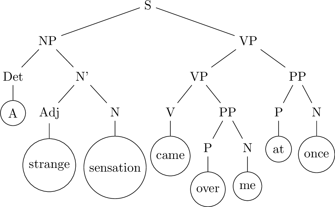
The Random Language Model is defined as follows [17]. A stochastic context-free grammar [11], [26], [27] is a generative model for sequences with a hidden tree structure; a grammar in Chomsky normal form defines a weight over binary trees, called derivations, in which the leaves of the tree represent the observed sequence; Fig. 1 shows an example derivation of English phrase structure. The grammar \(\mathcal{G}\) is defined by two objects \(\mathcal{G}= \{M_{abc}, O_{aB} \}\) over sets of hidden ("nonterminal") symbols indexed by \(a=1,\ldots,N\) and observable ("terminal") symbols indexed by \(B=1,\ldots,T\) such that the rule \(a \to bc\) has the weight \(M_{abc}\) and the rule \(a \to B\) has the weight \(O_{aB}\). Conventionally, each derivation begins with a distinguished symbol, called the start symbol, which is the root. The model of [17] defines weights for tree topologies based on a branching process with emission probability \(p_E\), so that a binary tree \(\mathcal{T}\) with \(\ell\) leaves has a probability \(\mathbb{P}(\mathcal{T}| \mathcal{G}) = W_{tree}(\mathcal{T})/Z_{tree}\) with \(W_{tree}(\mathcal{T}) = p_E^{\ell} (1-p_E)^{2\ell-1}\). The ‘emission probability’ \(p_E\) controls the size of trees ¹. The tree is defined by a set of interior branches \(\Omega_\mathcal{T}\) and surface branches \(\partial\Omega_\mathcal{T}\). The emission probability \(p_E\) needs to be tuned close to \(1/2^+\) to obtain large trees; if we write \(p_E = 1/2 + \varepsilon\) then the distribution of tree lengths is given by \(\mathbb{P}(\ell) \propto e^{-\ell/\xi}/\ell^{3/2}\) with \(\xi = 1/(4\varepsilon^2)\).

Given the topology of a tree, \(\mathcal{G}\) defines a weight for each derivation on it. Writing the hidden symbols of a particular derivation as \(\{\sigma_i\}\) and the observable symbols as \(\{ o_t \}\) the weight is \[\begin{align} \label{w1} W( \{\sigma_i, o_t \} | \mathcal{T}, \mathcal{G}) = \prod_{\alpha \in \Omega_\mathcal{T}} M_{\sigma_{\alpha_1} \sigma_{\alpha_2} \sigma_{\alpha_3} } \prod_{\alpha \in \partial\Omega_\mathcal{T}} O_{\sigma_{\alpha_1} o_{\alpha_2} }, \end{align}\tag{1}\] where each \(\alpha=(\alpha_1,\alpha_2,\alpha_3)\) is a factor in the order \(\sigma_{\alpha_1} \to \sigma_{\alpha_2} \sigma_{\alpha_3}\). We can write the weight in a Boltzmann form \[\begin{align} \label{w2} W( \{\sigma_i, o_t \} | \mathcal{T}, \mathcal{G}) = e^{-E}, \end{align}\tag{2}\] with \[\begin{align} E = - \sum_{\alpha \in \Omega_\mathcal{T}} \log M_{\sigma_{\alpha_1} \sigma_{\alpha_2} \sigma_{\alpha_3} } -\sum_{\alpha \in \partial\Omega_\mathcal{T}} \log O_{\sigma_{\alpha_1} o_{\alpha_2} } \end{align}\] We can write this as \[\begin{align} E & = -\sum_{a,b,c} \pi_{abc}(\sigma; \mathcal{T}) \log M_{abc} - \sum_{a,B} \rho_{aB}(\sigma,o; \mathcal{T}) \log O_{aB} \end{align}\] where the usage frequencies are \[\begin{align} \pi_{abc}(\sigma; \mathcal{T}) & = \sum_{\alpha \in \Omega_{\mathcal{T}}} \delta_{\sigma_{\alpha_1},a} \delta_{\sigma_{\alpha_2},b} \delta_{\sigma_{\alpha_3},c} \\ \rho_{aB}(\sigma,o; \mathcal{T}) & = \sum_{\alpha \in \partial\Omega_{\mathcal{T}}} \delta_{\sigma_{\alpha_1},a} \delta_{o_{\alpha_2},B} \end{align}\] For a given derivation, these quantities count how many times each grammar rule is used. The grammar can be written as \(\log M_{abc} = \log \overline{M} + \log M_{abc}/\overline{M} \equiv \log \overline{M} + X_{abc}\) and similarly \(\log O_{aB} = \log \overline{O} + Y_{aB}\). Using the sum rules \(\sum_{a,b,c} \pi_{abc} = |\Omega| = \ell - 1\) and \(\sum_{a,B} \rho_{aB} = |\partial\Omega| = \ell\) we can extract a mean contribution, independent of the configuration \(\sigma, o\). Thus \[\begin{align} E & = E_0 -\sum_{a,b,c} \pi_{abc}(\sigma; \mathcal{T}) X_{abc} - \sum_{a,B} \rho_{aB}(\sigma,o; \mathcal{T}) Y_{aB} \end{align}\] with \(E_0 = -(\ell-1) \log \overline{M} - \ell \log \overline{O}\). The partition function of derivations on a fixed tree and with a fixed grammar is \[\begin{align} Z(\mathcal{T},\mathcal{G}) = \sum_{\{ \sigma_i, o_t \} } W( \{\sigma_i, o_t \} | \mathcal{T}, \mathcal{G}) . \end{align}\] The above definitions are for a single grammar \(\mathcal{G}\). The Random Language Model is an ensemble of grammars in which the \(X_{abc}\) and \(Y_{aB}\) are drawn from a Gaussian distribution, iid for each rule, with variance \(1/(2\tilde{\epsilon}_d)\) and \(1/(2\tilde{\epsilon}_s)\) for \(X\) and \(Y\), respectively.

2 Field-theory of the Random Language Model↩︎

Here we recall the construction of [19], which builds a field theoretic representation of the RLM. We will use this field theory to show the breakdown of simple ‘paramagnetic’ saddle-point solutions, governed by the Random Energy Model. This discussion parallels that of [25], with the difference that here we use the formalism of [19], which will also be employed in later sections, while in [25] the conventional belief propagation equations [28] on a fixed tree were used ². In a first reading, this section can be skipped.

The main idea of the construction in [19] is to find a field theory whose Feynman diagrams generate exactly the syntax trees of the RLM, with the correct weights. Such a field theory will operate on a fixed grammar \(\mathcal{G}= \{M_{abc}, O_{aB} \}\) and thus be a disordered field theory. Note that the later sections of [19], which solve the model in the replica-symmetric approximation, contain a subtle error corrected in [29]. This does not affect the following discussion.

Fix a stochastic context-free grammar in Chomsky normal form \(\mathcal{G}= \{M_{abc}, O_{aB} \}\). We consider the partition function of \(m\) sentences with total length \(\ell\), which can be written as \[\begin{align} \mathbb{Z}(\mathcal{G}; m, \ell) = \sum_{\{\ell_i\}, \sum_{i=1}^m \ell_i = \ell} \prod_i \mathbb{Z}(\mathcal{G}; \ell_i) , \end{align}\] where the tree-averaged partition function for a single sentence of length \(\ell_i\) is \[\begin{align} \mathbb{Z}(\mathcal{G}; \ell_i) = \sum_{\mathcal{T}, \ell(\mathcal{T})=\ell_i} \mathbb{P}(\mathcal{T}| \mathcal{G}) Z(\mathcal{T},\mathcal{G}) . \end{align}\] We have \(\sum_{i} |\partial\Omega_{\mathcal{T}_i}| = \sum \ell_i = \ell\), and \(\sum_i |\Omega_{\mathcal{T}_i}| = \sum (2\ell_i-1) = 2\ell - m\), so that \(\mathbb{Z}_{tree} \equiv \prod_i \mathbb{P}(\mathcal{T}_i|\mathcal{G})=p_E^{\ell} (1-p_E)^{2\ell-m} Z_{tree}^{-m}\) just gives a trivial factor.

The first result of [19] is that \(\mathbb{Z}(\mathcal{G}; m,\ell)\) has a field-theoretic representation in terms of two complex scalar ‘fields’ \(L_a, R_a, a = 1,\ldots,N\) living on the space of hidden symbols. This takes the form \[\begin{align} \label{W2} \mathbb{Z}(\mathcal{G}; m, \ell) = m! \oint' \frac{d\zeta}{\zeta^{1+m}} \oint' \frac{d\xi}{\xi^{1+\ell}} \oint' \frac{d\eta}{\eta^{1+\ell-m}} \;\mathcal{F}(\mathcal{G}), \end{align}\tag{3}\] where \(\oint' = \oint/(2\pi i)\), where \[\begin{align} \mathcal{F}(\mathcal{G}) = \int DL \int DR \; e^{-\frac{1}{g} \sum_a \left[ L_a L_a^\dagger + R_a R_a^\dagger \right] } e^{I} , \end{align}\] where \({}^\dagger\) denotes complex conjugate and \[\begin{align} \label{I} I & = \zeta h (L_1+R_1) + \xi \sum_a O_a (L_a^\dagger + R_a^\dagger) \notag\\ & \qquad + \eta \sum_{a,b,c} M_{abc} (L_a^\dagger + R_a^\dagger) L_b R_c. \end{align}\tag{4}\] with \(O_a = \sum_B O_{aB}\). The measure \(DL=\prod_a d\text{Re}[L_a] d\text{Im}[L_a]/(\pi g)\) is normalized such that \(\int DL \; e^{-\frac{1}{g} \sum_a L_a L_a^\dagger} = 1\), and similarly for \(R\). The constants \(g\) and \(h\) are chosen to satisfy \((2h)^m g^{2\ell-m} = p_E^\ell (1-p_E)^{2\ell-m} Z_{tree}^{-m}\), i.e. \(g=\sqrt{p}(1-p), h=\sqrt{p}/(2Z_{tree})\).

Eq.@eq:W2 defines a complex-valued \(3+2N-\)component disordered field theory in 0 dimensions. The fact that the \(L_a,R_a\) fields are complex-valued corresponds to the trees being directed: roots are distinguished from leaves, and for example \(M_{abc}\) corresponds specifically to a branch from \(a \to bc\) that is aligned from root towards the leaves. This entails that the propagator of the field theory distinguishes ‘past’ from ‘future’, if we identify time as flowing from the root to the leaves.

It follows by a straightforward rescaling that in this representation, \(\mathbb{Z}(\mathcal{G}; m,\ell)\) is governed by a saddle-point when \(\ell \to \infty\) and \(m \to \infty\) at finite average sentence length \(\ell/m\). This is the limit of a large text. It is convenient to write \(H_a = L_a^\dagger+R_a^\dagger\) for a head. The saddle-point equations are \[\tag{5} \begin{align} L_a & = g \xi O_a + g \eta \sum_{b,c} M_{abc} L_b R_c \tag{6}\\ L_a^\dagger & = g h \zeta \delta_{a1} + g \eta \sum_{a',b,c} M_{a'bc} H_{a'} \delta_{ab} R_c \tag{7} \\ R_a & = g \xi O_a + g \eta \sum_{b,c} M_{abc} L_b R_c \tag{8} \\ R_a^\dagger & = g h \zeta \delta_{a1} + g \eta \sum_{a',b,c} M_{a'bc} H_{a'} L_b \delta_{ac} \tag{9} \\ \ell-m & = \eta \sum_{a,b,c} M_{abc} H_a L_b R_c \tag{10} \\ \ell & = \xi \sum_{a} O_a H_a \tag{11} \\ m & = \zeta h (L_1+R_1) \tag{12} \end{align}\] for all \(a\) ³.

Eqs.@eq:SP bear a formal resemblance to belief propagation equations [28], but they are not identical. The former are defined for one fixed tree, and in terms of quantities with fixed site indices. In contrast, here the fields are defined on the symbols, and the partition function that is generated automatically samples all tree topologies. Nevertheless, this identification allows us to interpret \(L_a\) and \(R_a\) as downward messages, while \(L^\dagger_a\) and \(R^\dagger_a\) are upward messages.

Subtracting the third equation from the first we see that \(R_a=L_a\) although the left-right symmetry does not hold for the conjugates, in general. We can however sum the \(L^\dagger\) and \(R^\dagger\) equations (after swapping \(b\) and \(c\) in the latter) to get \[\begin{align} H_a & = 2 g h \zeta \delta_{a1} + g \eta \sum_{a',c} [M_{a'ac} + M_{a'ca} ] H_{a'} L_c \label{SP8} \end{align}\tag{13}\] which is closed in \(H_a\) rather than \(L^\dagger_a\) and \(R^\dagger_a\) separately. This implies that unless we probe observables that break the left-right symmetry, we can reduce the theory by eliminating the \(R_a\) field.

Evaluating \(\mathbb{Z}(\mathcal{G}; m,\ell)\) on the saddle-point, we obtain to leading exponential order \[\begin{align} \left.\mathbb{Z}(\mathcal{G}; m,\ell)\right|_{SP} & = \frac{m!}{\zeta^m \xi^\ell \eta^{\ell-m}} e^{-\frac{1}{g} \sum L_a [L^\dagger_a+R^\dagger_a] } e^{m + \ell + \ell - m} \notag \\ & = \frac{m!}{\zeta^m \xi^\ell \eta^{\ell-m}} e^{-\frac{1}{g} g (2\ell-m) } e^{2\ell} \notag \\ & = \left( \frac{m \eta}{\zeta} \right)^m \left( \xi \eta \right)^{-\ell} \end{align}\] using \(\sum L_a [L^\dagger_a+R^\dagger_a] = \sum_a g \xi O_a H_a+ g \eta \sum_{b,c} M_{abc} H_a L_b R_c = g \ell + g (\ell-m) = g (2\ell-m)\). This expression for \(\mathbb{Z}\) includes the terms that give a finite limit in \(\lim_{m \to \infty} \log \mathbb{Z}/m\). Further simplification requires solution of the saddle-point equations.

2.1 REM approach↩︎

To establish the connection to the REM, consider the ‘paramagnetic’ ansatz \[\begin{align} L_a & = g \xi O_a + \bar L\\ H_a & = 2 g h \zeta \delta_{a1} + \bar H \end{align}\] so that the main equations above become \[\begin{align} \bar L & = g \eta \sum_{b,c} M_{abc} (g \xi O_b + \bar L) (g \xi O_c + \bar L) \\ \bar H & = g \eta \sum_{a',c} (M_{a'ca}+M_{a'ac}) (2g h \zeta \delta_{a'1} + \bar H ) (g \xi O_c + \bar L) \end{align}\] and we also have normalization equations for \(\eta,\xi,\) and \(\zeta\): \[\begin{align} \ell-m & = \eta \sum_{a,b,c} M_{abc} (2 g h \zeta \delta_{a1} + \bar H ) (g \xi O_b + \bar L)(g \xi O_c + \bar L) \\ \ell & = \xi \sum_{a} O_a (2 g h \zeta \delta_{a1} + \bar H ) \\ m & = 2\zeta h (g \xi O_1 + \bar L) \end{align}\] Let us make the simplifying assumption that \(O_1=0\), i.e. the start symbol never directly becomes an observable. In the general case this is a \(1/N\) correction that is irrelevant in the large \(N\) limit to be considered. Then \(\zeta = m/(2h\bar L)\) and \(\xi = \ell/(\bar H \sum_a O_a)\), and the \(\eta\) equation is trivially solved.

Now return to the main equations. The paramagnetic ansatz will close if the law of large numbers holds for all terms carrying a free index. We have the sums \[\begin{align} S_a^{(1)} &= \sum_{b,c} M_{abc} \\ S_a^{(2)} &= \sum_{b,c} M_{abc} O_b \\ S_a^{(3)} &= \sum_{b,c} M_{abc} O_c \\ S_a^{(4)} &= \sum_{b,c} M_{abc} O_b O_c \\ S_a^{(5)} &= \sum_{c} (M_{1ac}+M_{1ca}) \\ S_a^{(6)} &= \sum_{c} (M_{1ac}+M_{1ca}) O_c \end{align}\] which all take the form of a REM partition function but with different system sizes and variances. Let us write \[\begin{align} Z_{REM}(\mathcal{N},\lambda) = \sum_{j=1}^{\mathcal{N}} e^{-\beta E_j} \end{align}\] where \(\langle E_j \rangle = 0, \langle (\beta E_j)^2 \rangle = \lambda^2/2\). Derrida’s result is that the LLN breaks down when \[\begin{align} \frac{T}{T_c} = \frac{2\sqrt{\log 2}}{\beta J} = \frac{2\sqrt{\log \mathcal{N}}}{\lambda} \end{align}\] is smaller than unity. The corresponding parameters for the above sums are \[\begin{align} \mathcal{N}^{(1)} & = N^2, \lambda^{(1)} = \sqrt{1/\tilde{\epsilon}_d} \\ \mathcal{N}^{(2)} & = N^2 T, \lambda^{(2)} = \sqrt{1/\tilde{\epsilon}_d+ 1/\tilde{\epsilon}_s} \\ \mathcal{N}^{(3)} & = N^2 T, \lambda^{(3)} = \sqrt{1/\tilde{\epsilon}_d+ 1/\tilde{\epsilon}_s} \\ \mathcal{N}^{(4)} & = N^2 T^2, \lambda^{(4)} = \sqrt{1/\tilde{\epsilon}_d+ 2/\tilde{\epsilon}_s} \\ \mathcal{N}^{(5)} & = N, \lambda^{(5)} = \sqrt{1/\tilde{\epsilon}_d} \\ \mathcal{N}^{(6)} & = N T, \lambda^{(6)} = \sqrt{1/\tilde{\epsilon}_d+ 1/\tilde{\epsilon}_s} \end{align}\]

Note that, in the scaling limit, we have that all \(\lambda^{(i)} \sim \sqrt{\log N}\) while \(\sqrt{\log \mathcal{N}^i} \sim \sqrt{\log N}\) as well. Hence \(T/T_c\) is finite. The scaling limit of the RLM corresponds to the thermodynamic limit of the REM.

We see that the first breakdown will occur due to the root terms (i.e. those involving fixed symbol index 1), when \(\tilde{\epsilon}_d\log N < 1/4\) or \(\frac{\tilde{\epsilon}_d\tilde{\epsilon}_s}{\tilde{\epsilon}_d+\tilde{\epsilon}_s} \log NT < 1/4\). However it is not obvious whether the associated terms are actually relevant in the equations. A short calculation shows that, starting from the large \(\tilde{\epsilon}_d\) limit where all terms are self-averaging, the root terms have a relative weight \[\begin{align} \frac{2g h \zeta \delta_{a'1}}{\bar H} \sim \frac{m}{\ell-2m}, \end{align}\] which is finite as \(N \to \infty\) but suppressed for large trees, since \(\ell/m\) is the average length of a sentence.

After this first breakdown, which has a weak effect because it is suppressed by the average sentence length, the LLN will break down when \(S_a^{(1)}\) is not self-averaging; this occurs at \(\tilde{\epsilon}_d\log N = 1/8\). This sum controls the bulk propagation of messages and the breakdown of the LLN for it will destabilize the paramagnetic solution.

The result of the analysis is then the following: starting at large \(\tilde{\epsilon}_d\), for the bulk of the tree (i.e. for observables that do not depend on the terminals, and are therefore independent of \(\tilde{\epsilon}_s\) and \(T\)), a first weak breakdown will occur at \(\tilde{\epsilon}_d\log N = 1/4\), due to the influence of the start symbol. A complete breakdown will occur at \(\tilde{\epsilon}_d\log N = 1/8\).

For observables that depend on the terminals, the result depends on \(T/N\) and \(\tilde{\epsilon}_d/\tilde{\epsilon}_s\) but if \(\tilde{\epsilon}_s\) is fixed to be small (which is usually taken in the numerics, e.g. \(\tilde{\epsilon}_s= 0.01\)) then a weak breakdown will occur at \(\frac{\tilde{\epsilon}_d\tilde{\epsilon}_s}{\tilde{\epsilon}_d+\tilde{\epsilon}_s} \log NT = 1/4\), and a complete breakdown at \(\frac{\tilde{\epsilon}_d\tilde{\epsilon}_s}{\tilde{\epsilon}_d+\tilde{\epsilon}_s} \log (N^2T) = 1/4\).

These breakdowns are all of the LLN. As in the REM there will be corresponding breakdowns in the CLT at larger temperatures [30]. For a sum over \(N^K\) variables, the LLN breaks down at \(x_{LLN}=1/4K\) while the CLT breaks down at \(x_{CLT}=1/K\). Thus each CLT transition occurs at a value of \(x\) that is larger by a factor 4.

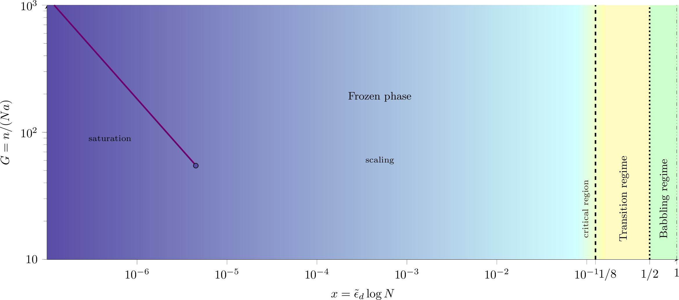
The phase diagram of the RLM is sketched in Fig.2, as a function of \(x\) and a scaling variable \(G=n/(Na)\) where \(a\sim \sqrt{8x}\) that will emerge from the analytical developments that follow as an effective corpus length. The transitions at \(x_c=1/8\) (dashed) and \(x=1/2\) (dotted) are indicated, delineating the frozen regime \(x<1/8\), the transition regime \(1/8 < x < 1/2\), and a ‘babbling’ regime \(x>1/2\). Further arguments (see [25]) indicate that \(x=1\) should also play a role as the initial onset of correlations in derivations, although it is not manifest in the bulk observables to follow here. It is indicated by a dash-dotted line.

The phase diagram has further structure to be elucidated in what follows: a critical regime near \(x_c=1/8\), and a saturation regime at small \(x\).

Although the field-theoretic approach locates the critical transitions, once the paramagnetic solution breaks down it is impractical to directly solve the full saddle-point equations. Fortunately, in the large \(N\) limit we can exploit a subtle self-averaging property of the model, as detailed next.

3 Scaling in the low-temperature regime↩︎

The above results indicate that at low temperature, there is a competition between increasing \(N\), which favours averaging, and lowering \(\tilde{\epsilon}_d\), which increases rule variance. This opens the possibility to take \(N \to \infty\) while also taking \(\tilde{\epsilon}_d\to 0\), such that \(\tilde{\epsilon}_d\log N\) remains finite. In this scaling limit, we can exploit simplifications due to large \(N\) while also retaining the ability to control entropy and other language properties, by tuning \(x = \tilde{\epsilon}_d\log N\). Similar considerations imply that we should fix \(y = \tilde{\epsilon}_s\log T\) to obtain nontrivial scaling in the surface properties.

We will consider this limit both for finite trees and in the limit of a large corpus; in the numerics of [17], trees were chosen by a branching process with \(\langle \ell \rangle \approx 15\). This of course does not preclude considering the limit of an infinite corpus.

Consider the partition sum of the RLM for a fixed forest \(\mathcal{F}\) of trees with lengths \(\{ \ell_i, i = 1 \ldots m \}\) and grammar \(\mathcal{G}\), which is written as a sum over trees \(\mathcal{T}_i\): \[\begin{align} \mathbb{Z}(\mathcal{F}; \mathcal{G}) = \prod_i Z(\mathcal{T}_i,\mathcal{G}) . \end{align}\] with \[\begin{align} Z(\mathcal{T},\mathcal{G}) = \underbrace{\overline{M}^{\ell-1} \overline{O}^\ell }_{Z_0(\ell)} \sum_{\{ \sigma_i, o_t \} } e^{-E'} \end{align}\] and \[\begin{align} E' = -\sum_{a,b,c} \pi_{abc}(\sigma; \mathcal{T}) X_{abc} -\sum_{a,B} \rho_{aB}(\sigma,o; \mathcal{T}) Y_{aB} . \end{align}\]

3.1 Excitations↩︎

Fix a forest \(\mathcal{F}\) and define the rule spectrum \(\{p_k, q_k, k \geq 1\}\) that for each \(k\) indicates how many rules are used \(k\) times, with \(p_k\) counting the number of hidden rules and \(q_k\) the number of terminal rules. For example, the derivation in Fig.1 has 7 branches, of which 2 use the same rule, so that \(p_1 = 5, p_2 = 1,\) and \(p_k=0\) for \(k \geq 3\), and \(q_1=8,q_k= 0\) for \(k \geq 2\). The set of all derivations consistent with a given spectrum is called a pattern, \(P(\{p_k,q_k\}; \mathcal{F})\).

The partition sum \(Z\) can be organized as a sum over patterns, which are the relevant excitations of the model: \[\begin{align} \mathbb{Z}(\mathcal{F}; \mathcal{G}) = \mathbb{Z}_0 \sum_{\{ P \}} \underbrace{\sum_{ (\sigma,o) \in P } e^{- E'(\sigma,o; \mathcal{G})}}_{\mathcal{P}(P; \mathcal{G})} , \end{align}\] where \(\mathbb{Z}_0 = \prod_i Z(\ell_i)\) depends only on the number of trees \(m\) and the total length \(\ell = \sum_i \ell_i\). For any derivation, applying a global permutation to the symbols results in another derivation with the same pattern, but different rules. Since the model is defined by iid rule weights, each pattern thus explores the space of grammars. In other words, even though \(\mathbb{Z}\) is computed for a fixed grammar, sums over symbol values amount to sums over possible grammar weights. This is a form of self-averaging, which we use to justify the semi-annealed approximation that follows. It is however essential to respect the rule spectrum of the pattern, since this controls the Boltzmann weight.

The organization of the partition function as a sum over patterns suggests a natural large-deviation structure. Each pattern \(P\) contributes a weight that combines an energetic term, controlled by the rule multiplicities, and a combinatorial entropy that counts the number of derivations realizing that spectrum. Crucially, both contributions diverge in the scaling limit (in particular both are powers of \(N\), as confirmed below). As a result, the partition function can be written \[\begin{align} \mathbb{Z}(\mathcal{F}; \mathcal{G})/\mathbb{Z}_0 = \sum_{\{ P \}} e^{S(P)} e^{-\hat{E}(P)} \end{align}\] where \(S(P)\) encodes the entropy of patterns and \(\hat{E}(P)\) is an effective energy after averaging over rule weights. In the scaling limit this will be dominated by a saddle point \(P_*\) that minimizes the effective free energy \(\hat{E}-S\). This provides a basis for a semi-annealed approximation: we perform an annealed average over rule weights within each pattern, while retaining the constraint that the pattern itself is selected by a saddle-point condition at fixed \(N\). In this sense, the approximation is not a fully annealed treatment of the original quenched problem, but rather a coarse-grained saddle-point evaluation over patterns, which captures the dominant contributions in the scaling limit.

This perspective also clarifies the role of the rule spectrum \(\{ p_k, q_k \}\) as an order-parameter-like object: different phases of the model correspond to qualitatively different saddle-point spectra, reflecting whether weight is distributed over many rules or concentrated onto a few. As we show below, this structure leads to a condensation transition analogous to that of the Random Energy Model.

There are two important ingredients to the semi-annealed approximation. First, since trees can be sampled sequentially from the root without backtracking, for a given head \(a\) there are \(N^2\) possible rules \(a \to bc\) to consider. This defines an elementary REM partition sum, one for each branch.

Second, although rule distributions are heavy-tailed at small \(\tilde{\epsilon}_d\), at any finite \(N\) we only sample a finite number of values from the distribution. Using extreme-value statistics, a sum over \(N^2\) variables sampled from \(P(M)\) will typically not see a value larger than \(M^*\) where \[\begin{align} \frac{1}{N^2} & = \int_{M^*}^\infty dM P(M) \notag \\ & = \int_{M^*}^\infty \frac{dM}{M\sqrt{\pi/\tilde{\epsilon}_d}} e^{-\tilde{\epsilon}_d\log^2 (M/\overline{M}) } \notag \\ & = \int_{X_*}^\infty \frac{dX}{\sqrt{\pi/\tilde{\epsilon}_d}} e^{-\tilde{\epsilon}_dX^2 } \notag \\ & = \frac{1}{2}\text{erfc}(\sqrt{\tilde{\epsilon}_d} X_*) \end{align}\] with \(X=\log (M/\overline{M})\) and \(X_* = \log (M^*/\overline{M})\). Define an average restricted to the interval \(M<M^*\), or equivalently \(X<X_*\): \[\begin{align} \langle f(X) \rangle_{X<X_*} = \frac{\int_{-\infty}^{X_*} dX P(X) f(X)}{\int_{-\infty}^{X_*} dX P(X)} \end{align}\] Then in the semi-annealed approximation, a pattern contributes \[\begin{align} \label{P} \mathcal{P}(\{p_k, q_k\}) = \underbrace{\left. \Omega N^Q T^{Q'} \right. }_{e^S} \underbrace{\prod_k \langle e^{k X} \rangle_{X<X_*}^{p_k} \prod_{k'} \langle e^{k' Y} \rangle_{Y<Y_*}^{q_{k'}} }_{e^{-\hat{E}}} \end{align}\tag{14}\] where \(Q\) and \(Q'\) count the number of DOF in the average over symbols, and \(\Omega\) accounts for the entropy of the pattern.

3.2 Pattern entropy↩︎

Exact counting of derivations is difficult in large trees, but we can obtain a simple estimate by counting degrees of freedom. We consider a forest of \(m\) trees, of total length \(\ell\). There are \(n= \ell-m\) branches. We have \(n = \sum_k k p_k\) and \(\ell = \sum_k k q_k\). The total number of unique hidden rules used in the pattern is \(p = \sum_j p_j\), while \(q= \sum_j q_k\) is the total number of unique terminal rules. Eventually we will need to decide on the relative size of \(\ell\) and \(N\).

First choose the symbols used by the \(p\) branching rules; this gives \(\binom{N^3}{p} \sim N^{3p}/p!\) if \(N^3 \gg p\). The first correction is a factor \(e^{-p^2/2N^3}\) that will be negligible if \(p \ll N^3\).

Then distribute these according to the rarity distribution; this gives a multinomial coefficient \[\begin{align} \binom{p}{p_1 \; p_2 \; \cdots }. \end{align}\]

Having fixed the identities of the rules, we can then create different derivations by placing them in different configurations. This can be estimated due to two simplifying factors of the model: first, the tree structure allows configurations to be built sequentially, starting from the root, without backtracking. Second, since all rules are iid, if for example we have a rule \(a \to bc\), then the likelihood of having a rule whose head is \(b\) is independent of the value \((a)\) of the head. Thus, suppose we have a pile of \(\ell_c\) rules, of which \(p\) of them are unique. We assume that \(\ell_c/p\) is large, so that a typical rule appears frequently. Then, starting from the root, we will have typically \(p/N\) rules with the start symbol as head. Continuing to its children, we will have \(p/N\) choices for the next branch, and so on. This yields a simple estimate \((p/N)^{\ell_c}\) for the number of unique derivations. It implies that the pile will yield a unique derivation if \(p \approx N\).

This estimate is refined by an exact calculation based on Eqs.@eq:SP (see Appendix 11). It confirms the \((p/N)^{\ell_c}\) result and applies even when \(p<N\), when the above argument is unreliable; indeed an analysis of corrections to the leading order reveals that the estimate works best when \(p/N\) is small and when the total corpus length is small.

However, this estimate does not account for the depletion of rules as we build derivations. We account for this by dividing up the full \(n\) rules (counted with multiplicity) into piles of \(\ell_c\) rules, each of which has \(N\) unique rules. Each pile will then typically have a unique derivation. Since the average repetition rate of a rule is \(n/p\) we take \(\ell_c = n N/p\), and hence \(m_c = p/N\) piles, which play the role of correlation volumes. This requires \(p/N\geq 1\), since \(m_c\) must be integer.

For \(p>N\), counting derivations thus reduces to counting the number of ways to partition the initial \(n\) rules (with given multiplicity spectrum) into \(m_c\) correlation volumes. Label the volumes 1 through \(m_c\) and consider each rule type \(r\), i.e. triple \(r= (a,b,c)\) corresponding to \(a \to bc\). Suppose this rule occurs \(\pi\) times in the complete pile of \(n\) rules. Then there are \(\binom{\pi + m_c - 1}{m_c -1}\) ways to put these \(\pi\) rules into the correlation volumes. Repeating this for all rules and recalling the definitions of \(\{ p_k \}\) we find ⁴ \[\begin{align} \prod_{k \geq 1} \binom{k + m_c - 1}{m_c -1}^{p_k} . \end{align}\] As a result, counting derivations gives a factor \[\begin{align} \label{OmD1} \Omega_D = \begin{cases} (p/N)^{n} &\qquad p/N<1 \\ \prod_{k \geq 1} \binom{k + m_c - 1}{m_c -1}^{p_k} &\qquad p/N>1 \end{cases} \end{align}\tag{15}\]

Now we choose and place the terminal rules. Consider the hidden symbols as given, for any particular realization of the pattern. We first need to know how many unique hidden symbols there are that become leaves; this depends on the topology of the tree. It is easily seen that the number is between \(p\) (if the tree always branches to the right, say) and \(2p\) (if the tree is fully balanced). For the branching process considered in the model, the typical value is \(3p/2\), as can be seen by a generating function argument.

We will assume that \(3p/2 > N\), so that all hidden symbols are represented. Then, the argument is very similar: first we choose the rules, \(\binom{NT}{q} \sim (NT)^q/q!\) if \(q \ll NT\); then we distribute these according to the rarity distribution, giving a multinomial coefficient \(\binom{q}{q_1 q_2 \cdots }\). Then we need to count sequences that are compatible. For each hidden symbol that becomes a leaf, there are typically \(q/N\) terminal rules that are compatible. Thus, as before we estimate \((q/N)^\ell\) sequences if rule depletion is ignored. Taking into account rule depletion, we split the \(\ell\) rules (counted with multiplicity) into \(m_c'\) piles of \(\ell_c'\) rules each. If each pile has \(N\) unique rules, then there will typically be one compatible sequence, which leads to \(\ell_c' = \ell N/q\) and \(m_c' = q/N\). Finally we need to count the number of ways to put the rules into piles. The result from counting sequences is a factor \[\begin{align} \label{OmpD1} \Omega_D' = \begin{cases} (q/N)^{\ell} &\qquad q/N<1 \\ \prod_{k \geq 1} \binom{k + m_c' - 1}{m_c' -1}^{q_k} &\qquad q/N>1 \end{cases} \end{align}\tag{16}\] We then obtain a simple estimate of the number of derivations as \[\begin{align} \label{S1} e^S & = \Omega N^Q T^{Q'} \notag\\ & = \binom{p}{p_1 p_2 \cdots } \frac{1}{p!} \binom{q}{q_1 q_2 \cdots } \frac{1}{q!} \Omega_D \Omega_D' N^{3p} (NT)^q, \end{align}\tag{17}\] with \(m_c=p/N\) and \(m_c'=q/N\), so that \(Q = 3p+q, Q' = q\). Note that \(\Omega\) also depends on \(N\) through \(m_c\).

3.3 Pattern energy↩︎

The effective energies of patterns depend on \(g_k=\langle e^{k X} \rangle_{X<X_*}\) and \(h_k=\langle e^{k Y} \rangle_{Y<Y_*}\). We have \[\begin{align} g_k = \langle e^{k X} \rangle_{X<X_*} & = \frac{\int_{-\infty}^{X_*} dX P(X) e^{kX } }{\int_{-\infty}^{X_*} dX P(X)} \notag\\ & = \frac{\int_{-\infty}^{X_*} dX e^{kX } e^{-\tilde{\epsilon}_dX^2} }{\int_{-\infty}^{X_*} e^{-\tilde{\epsilon}_dX^2} } \notag\\ & = \frac{ e^{k^2/(4\tilde{\epsilon}_d)} \text{erfc}((k-2\tilde{\epsilon}_dX_*)/\sqrt{4\tilde{\epsilon}_d} ) }{ 2 - \text{erfc}(\sqrt{\tilde{\epsilon}_d} X_*) } \end{align}\] We can simplify this expression, and that for \(X_*\), in the scaling limit. We use the continued fraction representation \[\begin{align} \text{erfc}(z) = \frac{z}{\sqrt{\pi} } e^{-z^2} \frac{1}{z^2+h(z)} \end{align}\] where \(h(z) = 1/2 + \ldots\) for \(z \gg 1\). (For \(z \ll -1\) we can use erfc\((z)=2-\text{erfc}(-z)\))

First, at large \(N\) we have that \(\text{erfc}(\sqrt{\tilde{\epsilon}_d} X_*) = 2/N^2 \ll 1\) so that we can use its asymptotics to obtain \(e^{-\tilde{\epsilon}_dX_*^2}/\sqrt{\tilde{\epsilon}_dX_*^2} \approx \sqrt{4\pi}/N^2\), which is solved \[\begin{align} 2 \tilde{\epsilon}_dX_*^2 = W_0(N^4/(2\pi)) \equiv w \sim \log(N^4/(2\pi)) \end{align}\] where \(W_0\) is a branch of the Lambert-\(W\) function satisfying \(W(z)e^{W(z)}=z\). Note then that \[\begin{align} \tilde{\epsilon}_dX_* = \sqrt{\tilde{\epsilon}_d} \sqrt{\tilde{\epsilon}_dX_*^2} \sim \sqrt{2 \tilde{\epsilon}_d\log N}, \end{align}\] which is finite in the scaling limit. As a result, the argument to \(\text{erfc}\) in \(g_k\) is large in magnitude (since \(\tilde{\epsilon}_d\ll 1\)) but may take either sign. We then have \[\begin{align} g_k& \sim \frac{1}{2}e^{k^2/(4\tilde{\epsilon}_d)} \begin{cases} 2 & k < 2 \tilde{\epsilon}_dX_* \\ \frac{ e^{ -(k-2\tilde{\epsilon}_dX_*)^2/(4\tilde{\epsilon}_d) } }{ \sqrt{\pi} (k-2\tilde{\epsilon}_dX_*)/\sqrt{4\tilde{\epsilon}_d}} & k > 2 \tilde{\epsilon}_dX_* \end{cases} \\ & = \begin{cases} e^{k^2/(4\tilde{\epsilon}_d)} & k < 2 \tilde{\epsilon}_dX_* \\ \frac{ e^{ (4k\tilde{\epsilon}_dX_* - 4\tilde{\epsilon}_d^2 X_*^2)/(4\tilde{\epsilon}_d) } }{ (k-2\tilde{\epsilon}_dX_*) \sqrt{\pi/\tilde{\epsilon}_d} } & k > 2 \tilde{\epsilon}_dX_* \end{cases} \end{align}\] The asymptotics depend on \(k\): for any given value of \(x\), rules that are repeated often enough will feel the effect of finite \(N\).

The surface terms are analogous. Define \(Y_*\) as the solution to \(2\tilde{\epsilon}_sY_*^2 = W_0(T^2/(2\pi)) \equiv w'\). We have \[\begin{align} h_k & = \frac{1}{2 - \text{erfc}(\sqrt{\tilde{\epsilon}_s} Y_*)} e^{k^2/(4\tilde{\epsilon}_s)} \text{erfc}\left( \frac{k-2\tilde{\epsilon}_sY_*}{\sqrt{4\tilde{\epsilon}_s}} \right) \\ & \sim \begin{cases} e^{k^2/(4\tilde{\epsilon}_s)} & k < 2 \tilde{\epsilon}_sY_* \\ \frac{ e^{ (4k\tilde{\epsilon}_sY_* - 4\tilde{\epsilon}_s^2 Y_*^2)/(4\tilde{\epsilon}_s) } }{ (k-2\tilde{\epsilon}_sY_*) \sqrt{\pi/\tilde{\epsilon}_s} } & k > 2 \tilde{\epsilon}_sY_* \end{cases} \end{align}\] This structure completely parallels that of the hidden layers, but note that \(w\) depends on \(N^4\) while \(w'\) depends on \(T^2\).

It is useful to note that \(e^{-\tilde{\epsilon}_dX_*^2} = \sqrt{2\pi w}/N^2\) with \(w = W_0(N^4/2\pi)\) and similarly \(e^{-\tilde{\epsilon}_sY_*^2} = \sqrt{2\pi w'}/T\) with \(w' = W_0(T^2/2\pi)\).

The Lambert-\(W\) function appears repeatedly in what follows. Defined by \(W(z) e^{W(z)} = z\), it has two branches: the \(W_0\) branch exists for \(z > -1/e\), behaves as \(W_0(z) \sim z\) as \(z\to 0\) and has large \(z\) behavior \(W_0(z) \sim \log z - \log \log z\). The second branch \(W_{-1}(z)\) exists for \(-1/e < z < 0\) and has asymptotics \(W_{-1}(z) \sim (\log -z) - (\log (-\log -z))\) for \(|z| \ll 1\). For \(z<-1/e\) neither \(W_0(z)\) nor \(W_{-1}(z)\) exist.

Below we will see frequent appearance of the quantities \[\label{aap} \begin{align} a & \equiv \sqrt{2 w \tilde{\epsilon}_d} \sim \sqrt{8 (\log N) \tilde{\epsilon}_d} = \sqrt{8x} \\ a' & \equiv \sqrt{2 w' \tilde{\epsilon}_s} \sim \sqrt{4 (\log T) \tilde{\epsilon}_s} = \sqrt{4y} \end{align}\tag{18}\] Note also that \(2 \tilde{\epsilon}_dX_* = \sqrt{2\tilde{\epsilon}_d} \sqrt{2 \tilde{\epsilon}_dX_*^2} = \sqrt{2\tilde{\epsilon}_dw} = a\) and \(2 \tilde{\epsilon}_sY_* = \sqrt{2\tilde{\epsilon}_sw'} = a'\).

If we define integers \(r,s\) such that \[\begin{align} & r < a < r+1 \\ & s < a' < s+1 \end{align}\] then we can write \[\begin{align} \label{gk1} g_k \sim \begin{cases} N^{\frac{k^2}{4x}} & k \leq r \\ N^{-2 + \frac{k a}{2x} } \frac{ a }{ k-a } & k > r \end{cases} \end{align}\tag{19}\] and \[\begin{align} \label{hk1} h_k \sim \begin{cases} T^{\frac{k^2}{4y}} & k \leq s \\ T^{-1 + \frac{k a'}{2y} } \frac{ a' }{ k-a' } & k > s \end{cases} \end{align}\tag{20}\] which give the energetic contribution \[\begin{align} \label{Ehat1} e^{-\hat{E}(P)} = \prod_k g_k^{p_k} h_k^{q_{k}} \end{align}\tag{21}\] Eqs.@eq:gk1 ,20 show explicitly that in the scaling limit, the energetic contributions have singular behavior at a whole array of temperatures, just as in the REM [24]. In particular, whenever \(a\) or \(a'\) is a positive integer, then one of the above asymptotics changes form.

3.4 Scaling in the large\(-N\) limit↩︎

We have now all the ingredients for the semi-annealed approximation. Eqs.@eq:OmD1 ,16 ,17 give the entropic part while Eqs.@eq:aap ,19 ,20 ,21 give the energetic part.

Consider initially a finite tree so that all \(p_k\) and \(q_k\) are finite. Also, for simplicity, consider \(r=s=0\), that is \(a <1, a' <1\), which corresponds to \(8x<1, 4y<1\) in the scaling limit. Then the leading behavior of the pattern weight is \[\begin{align} \mathcal{P}( \{p_k, q_k \}) &\sim N^{3p+q} T^q \prod_k \left( N^{-2 + \frac{k a}{2x} } \right)^{p_k} \left( T^{-1 + \frac{k a'}{2y} } \right)^{q_k} \\ &= N^{p+q + \frac{n a}{2x}} T^{\ell a'/2y} \\ &\sim N^{p+q+ n \sqrt{2/x}} T^{\ell \sqrt{1/y} } . \end{align}\] As alluded to above, all contributions diverge in the scaling limit. Similar to other defect models, such as the XY model [31]–[34], the weight of excitations depends on the temperature(s). When the multinomial factors of \(e^S\) are included, this implies that rule spectra will have preferred forms in the scaling limit. Hence there is a dominant pattern at each given \(\tilde{\epsilon}_d,\tilde{\epsilon}_s\).

In what follows, we extract the dominant patterns and their properties. First, we do so in finite trees, and then in large corpora; our goal throughout is to extract the leading asymptotic forms of observables in the scaling limit. These will be compared with direct numerical simulations and will be applied to data from real languages in subsequent sections.

3.5 Dominant rule spectrum↩︎

In the scaling limit there will be a preferred spectrum of rule multiplicities. We have \(p = \sum_k p_k,q = \sum_k q_k, n = \ell-m = \sum_k k p_k, \ell = \sum_k k q_k\). First consider the \(\{ p_k \}\); the hidden and surface spectra are decoupled so long as \(p/N>2/3\), which can be verified later. We maximize \(\mathcal{P}\) with a Lagrange multiplier \(\tilde{n}\) that imposes \(n = \sum_k k p_k\). Using the Stirling approximation for \(p_k!\) we obtain \[\begin{align} p_k = N^3 g_k e^{- k \tilde{n}} e^{\partial_{p_k} \log \Omega_D} \end{align}\] where \(\tilde{n}\) is fixed by \[\begin{align} n & = \sum_k k N^3 g_k e^{- k \tilde{n}} e^{\partial_{p_k} \log \Omega_D} \end{align}\] This depends both on the corpus size and on the behavior of the \(g_k\), which in turn depends on \(x\). We find \[\begin{align} \label{pk} p_k = \begin{cases} N^3 g_k e^{- k \tilde{n}} e^{n/p} \qquad\qquad & p<N \\ v \binom{k + m_c - 1}{m_c -1} N^3 g_k e^{- k \tilde{n}} \qquad\qquad & p>N \end{cases} , \end{align}\tag{22}\] with \(m_c=p/N\) and \(v = e^{\sum_{k'} \frac{p_{k'}}{N} \log \left(1+\frac{k'}{m_c-1}\right)}\).

Note that \(p\) is determined self-consistently from the solution, so we do not know in advance which regime we are in. However, if consider a single tree in the scaling limit, then we can expect \(p < N\), while if we consider a corpus of diverging size, then it is possible (and likely) to have \(p>N\).

The surface terms are analogous. The most likely pattern satisfies \[\begin{align} q_k = NT h_k e^{- k \tilde{m}} e^{\partial_{q_k} \log \Omega'_D} \end{align}\] This gives \[\begin{align} \label{qk} q_k = \begin{cases} NT h_k e^{- k \tilde{m}} e^{\ell/q} \qquad\qquad & q<N \\ v' \binom{k + m_c' - 1}{m_c' -1} NT h_k e^{- k \tilde{m}}\qquad\qquad & q>N \end{cases} , \end{align}\tag{23}\] with \(m_c' = q/N\) and \(v' = e^{\sum_k \frac{q_k}{N} \log (1+k/(m_c'-1))}\). \(q=\sum_k q_k\) must be determined self-consistently, and \(\tilde{m}\) is fixed implicitly by the constraint \(\ell = \sum_k k q_k\).

4 Rule use in finite trees↩︎

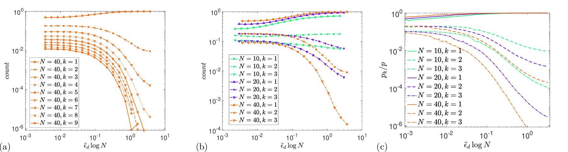
First consider a single finite tree in the scaling limit. Then since \(p\leq\ell\) while \(N\) diverges, we use Eq.@eq:pk with \(p<N\). We need to find \(\tilde{n}\) such that \(n=\sum_k k p_k\), and \(p\) such that \(p =\sum_k p_k\). The result for \(n=20\) is shown in Fig.3c and compared to sampled data from the RLM, where \(n\) is dynamical with \(\langle n \rangle \approx 16\), without fitting parameters. It captures all the features of the data.

We can obtain analytical approximations for the full spectrum in several regimes, as detailed in Appendix 13. In the frozen regime \(x<1/8\) we have \[\begin{align} p_k \approx N a z^k e^{n/p} /(k-a) \end{align}\] with \(z = N^{a/2x} e^{-\tilde{n}}\). In terms of \(G = n/Na\) we find \(z \approx 1 - e^{W_{-1}( -1/\log G )}\). At small \(x\), \(a \ll 1\), \(G \gg 1\) and \(z \to 1^-\), so that \(p_k/p \propto z^k/k\) is asymptotically independent of \(x\). This is observed in the data (Fig.3ab) for \(x \lesssim 10^{-2}\).

For \(x>1/8\) we find \(p \approx n\), that is, all rules are used uniquely. The \(x\) dependence of \(p_k\) does not have a simple form, but analytical approximations are available.

5 Rule use in a large corpus↩︎

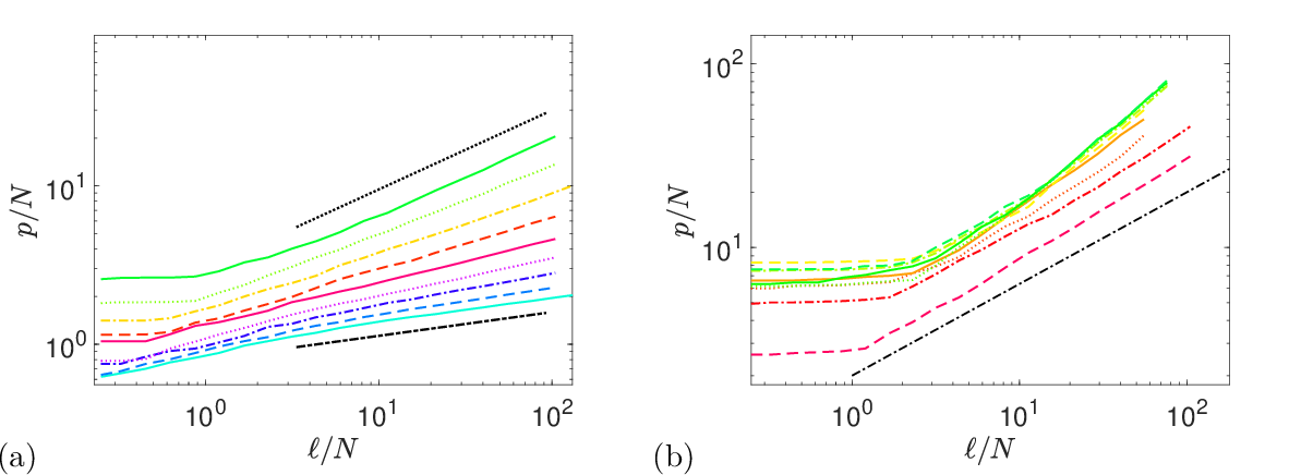
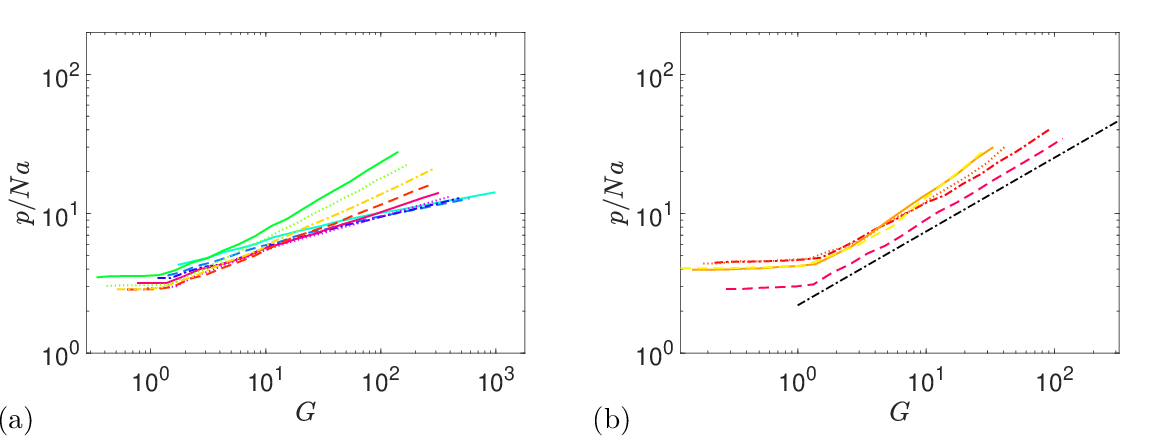
Now consider the opposite regime where \(p/N>1\). First, we present numerical data from the RLM at various \(N\), \(\tilde{\epsilon}_d\), and \(n\). Fig.4a shows the number of unique rules that appear in a corpus of total length \(\ell=n+m\), versus \(n/N\), at various \(x=\tilde{\epsilon}_d\log N\) in the frozen regime. Rules are counted over complete sentences; the plateau at small \(\ell\) corresponds to the typical number of unique rules in one sentence. Beyond this, \(p\) is approximately power-law in \(\ell\), with a ‘novelty’ exponent that changes continuously as \(x\) varies. Heavy dotted and dash-dotted lines indicate powers \(\ell^{0.5}\) and \(\ell^{0.15}\), respectively. This indicates that the language continues to exhibit novelty as corpus length grows, and the novelty rate depends upon the temperature \(\tilde{\epsilon}_d\). At smaller temperatures, the increase of novelty with corpus length is slower. Above \(x>1/8\), shown in Fig.4b, the pattern is similar: the dash-dotted line indicates a power \(\ell^{0.5}\).

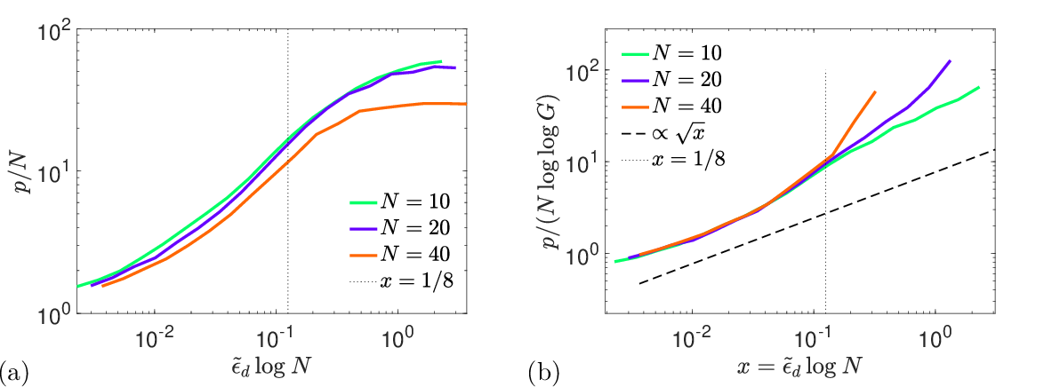
The \(N\) dependence is shown in Fig.5, at \(n \approx 850\) which is the upper limit where we have data across all values of \(x\) and \(N\). The leading dependence is \(p \propto N\) at finite \(x=\tilde{\epsilon}_d\log N\); a remaining weak dependence is collapsed by rescaling with a factor of \(\log \log G\), with \(G = n/(Na)\), as shown in Fig.5b. As a function of \(x\) we have approximately \(p/N \propto \sqrt{x} \log \log G\) in the frozen regime, at small \(x\). Theory should be able to rationalize all these scalings.

From Eqs.@eq:gk1 ,22 we can solve the model in the frozen regime, explained in Appendix 14, and obtain the phase diagram of the RLM, shown in Fig.2 in terms of the scaling variables \(x = \tilde{\epsilon}_d\log N\) and \(G = n/(Na)\). These are rescaled temperature and corpus-size parameters, respectively. \(G\) emerges from the solution of the equations, explained in what follows. Here \(a = \sqrt{2 w \tilde{\epsilon}_d} \sim \sqrt{8x}\).

Note that \(a/\sqrt{8x} = \sqrt{w/4\log N} \approx \sqrt{1 - \frac{\log \log N^4}{\log N^4} } \approx 0.90\) for \(N=40\), so there is a slight but measureable difference between \(a\) and its large-\(N\) asymptotic form \(\sqrt{8x}\).

5.1 Frozen regime↩︎

Within the frozen phase \(x<1/8\), we find three regimes: a saturating regime for \(x<x_{lo}\), a scaling regime for \(x_{lo}<x \ll 1/8\), and a critical regime when \(x \approx 1/8\). The scaling regime is where increasing the corpus size still realizes new rules, and the critical regime is where condensation is just occurring and rule use increases rapidly. In the saturating regime the number of rules used per symbol becomes small, and the semi-annealed theory breaks down.

We find the onset to saturation occurs at \[\begin{align} \label{xlo} x_{lo} = \frac{1}{8} \left( 8 \pi e^2 \right)^{-8/3} (n/N)^{-10/3} \end{align}\tag{24}\] Noting that \(\frac{1}{8} \left( 8 \pi e^2 \right)^{-8/3} \approx 1.1 \times 10^{-7}\), even at finite \(n/N\) this predicts a very small value of \(x_{lo}\), not visible in our numerics.

The number of unique rules per symbol is: \[\begin{align} p/N \approx \begin{cases} \frac{2}{3} a \sqrt{2\pi e^3} \log(3/2k_*) G^{\beta(G)} \qquad & x_{lo}< x \ll 1/8 \\ a \sqrt{2\pi e} e^{4 + \frac{3}{k_*-a} } \frac{ 1 }{k_*-a} \qquad & x \approx 1/8^- \end{cases} , \end{align}\] where \[\begin{align} \beta(G) \approx \frac{2}{1+\log G^{2/3} \log \log G^{2/3}} \end{align}\] is the novelty exponent, and \[\begin{align} k_* \approx \begin{cases} 3 (2\log (\log G^{2/3} \log \log G^{2/3}))^{-1} \qquad & x_{lo} < x \ll 1/8 \\ \frac{3}{4} + \frac{1}{2}a + \frac{1}{2}\sqrt{a^2 + a + \frac{9}{4}} \qquad & x \approx 1/8^- \end{cases} . \end{align}\] All results hold only for \(G\) in an intermediate range where the semi-annealed saddle exists. When \(G\) is too small, or potentially too large, rule use may be affected by the finiteness of the rule-set or the corpora. These implied thresholds are sensitive to corrections to the theory and therefore not well-predicted by the leading order solution that we consider.

For later use we have auxiliary variables \[\begin{align} z \approx k_* e^{3/2k_*} N/p \qquad & x_{lo} < x < 1/8 \end{align}\] and \[\begin{align} v \approx e^{k_*} \qquad & x_{lo} < x < 1/8 \end{align}\] In the scaling regime these can also be written in terms of \(\alpha \approx e^{3/2k_*}\).

Note that the four quantities \(N,\tilde{\epsilon}_d, p, n\) appear only in the three combinations \(p/N, n/N,\) and \(\tilde{\epsilon}_dw \sim \tilde{\epsilon}_d\log N\). This indicates that the scaling limit should be taken with \(n/N\) fixed and that \(p \propto N\) in this limit. This leading \(N\)-dependence of \(p\) is observed in Fig.5a.

The scaling regime is so-called because there, we have a further reduction to only two key combinations of parameters: \(p/Na\), and \(G=n/Na\). These results explain observations of Figs.4,5:

First, the predicted scaling collapse of \(p/Na\) versus \(G\) is tested in Fig.6a, where curves for \(x< 0.012\) collapse over the full range of \(G\), up to a small factor. At larger \(x\), the curves peel off when the critical regime becomes relevant. This lower function is the envelope valid for small enough \(x\). Note moreover that the raw \(p/N\) curves span a vertical range of \(6-10\) in Fig.4a, collapsed down to \(1.3-3\) here, even without accounting for critical regime effects to be understood later.

Second, the term \(G^{\beta(G)}\) explains the behavior \(p \sim n^{\beta(x)}\) with continuously changing exponent \(\beta(x)\), observed in Fig. 4a. Since \(\beta(G)\) decreases as \(G\) increases, the term \(G^{\beta(G)}\) predicts a concave shape of the envelope, as observed in Fig.6a. Third, since \(G^{\beta(G)} \sim e^{\frac{2 }{\log\log(G) }} \to 1\) at large \(G\), in this regime Eq.@eq:mc2 predicts that the \(N\)-dependence of \(p\) is fully captured by \(p \propto N \log\log G\), ignoring the ultra-slow \(\log\log\log G^{2/3}\) factor. This is confirmed in Fig.5b.

Fourth, Eq.@eq:mc2 predicts \(p/N \propto a \sim \sqrt{8x}\) in the scaling regime, confirmed in Fig.5b.

The critical regime is similar to the scaling regime, except that \(\beta(G)\) effectively increases, reaching a value \(\beta_c \approx 2/(1+e) \approx 0.537..\). This explains the scaling seen in Fig.4a as \(x \to 1/8^-\) and more generally the upturn visible in Fig.5b and Fig.6a.

Overall, the theory captures the scaling dependence of \(p\) on \(n\), \(N\), and \(x\) in surprising detail.

5.2 Transition regime↩︎

For \(x>1/8\), the asymptotics of small-\(k\) values of \(g_k\) differ. In Appendix 14 we obtain analytical approximations here, with the result \[\begin{align} p/N \approx \begin{cases} \frac{1}{2}N^{\chi } G^{1/2} \log G \qquad & n/N \gg N^{2\chi} \\ n/N \qquad & n/N \ll N^{2\chi} \end{cases} \end{align}\] where \(\chi(x) = 2 + \frac{1}{4x} - \sqrt{\frac{2}{x}}\). The scaling limit is taken at fixed \(n/N\) while \(N \to \infty\), so asymptotically we predict that \(p \approx n\) for \(x>1/8\) and all rules are used uniquely. In practice however we can see the other regime in numerics; the prediction \(p/N \sim G^{1/2}\) is observed, see Fig.6b.

For later use we will need \[\begin{align} z \approx N^{-\chi} e^{-G/A} \end{align}\] and \(v \approx e^{-G/A}\), for \(N^{2\chi} \gg n/N\).

6 Surface layer↩︎

The surface layer is solved analogously. It is decoupled (provided \(p/N>2/3\) as assumed) due to the hidden feedforward nature of the sequences along the hierarchical dimension. Comparing \(p_k\) in Eq.@eq:pk to \(q_k\) in Eq.@eq:qk and \(g_k\) in Eq.@eq:gk1 to \(h_k\) in Eq.@eq:hk1 , they are mathematically isomorphic. Results from the hidden layer can lifted by mapping \[\begin{align} a & \to a' \\ p_k/N &\to q_k/N \\ m_c &\to m_c' \\ v &\to v' \\ n/N &\to \ell/N \\ N &\to T^{1/2} \\ x &\to \frac{1}{2}y \end{align}\] This implies that we will have a control parameter \[\begin{align} G' = \frac{\ell/N}{a'} . \end{align}\] The existence and qualitative similarity of the RLM transition obtained as a function of \(\tilde{\epsilon}_s\), rather than \(\tilde{\epsilon}_d\), was shown in [22].

7 Thermodynamics↩︎

Now let us evaluate the partition function \(Z\) in the semi-annealed approximation. We work in the limit of a large corpus. Initially we consider only the hidden variables (WLOG). For given \(n\), the most likely pattern gives a weight (including its entropy)

\[\begin{align} & \Omega_D \frac{1}{p!} \binom{p}{p_1 p_2 \cdots } \prod_k \left( N^{3} g_k \right)^{p_k} \notag \\ & \qquad = \frac{1}{p!} \binom{p}{p_1 p_2 \cdots } \prod_k \left( e^{\tilde{n} k} p_k v^{-1} \right)^{p_k} \notag\\ & \qquad \approx e^{\tilde{n} n} \prod_k \frac{p_k^{p_k} }{(p_k/e)^{p_k}} v^{-p_k} \notag\\ & \qquad = e^{\tilde{n} n} e^p v^{-p} \notag\\ & \qquad = e^{\tilde{n} n} e^{p-p \log v} \end{align}\] where we used the Stirling approximation \(p! \approx (p/e)^p\) and only kept leading terms (in keeping with the previous use of Stirling).

The surface terms are completely analogous and give a contribution \(e^{\tilde{m} \ell + q \log e/v'}\). Finally in the semi-annealed approximation we estimate \[\begin{align} \mathbb{Z}(\mathcal{F}; \mathcal{G}) \approx \overline{M}^{\ell-m} \overline{O}^\ell e^{\tilde{n} (\ell-m) + p \log e/v} e^{\tilde{m} \ell + q \log e/v'} \end{align}\] We now apply the scaling symmetry of the model to restore \(\beta\) [22]; this amounts to making replacements \(\overline{M} \to \overline{M}^\beta, \overline{O} \to \overline{O}^\beta, \tilde{\epsilon}_d\to \tilde{\epsilon}_d/\beta^2, \tilde{\epsilon}_s\to \tilde{\epsilon}_s/\beta^2\).

We extract the energy and Boltzmann entropy from \[\begin{align} \langle E \rangle & = -\partial\langle \log \mathbb{Z}\rangle/\partial\beta|_{\beta=1} \\ \langle S_{Bol} \rangle & = \langle \log \mathbb{Z}\rangle + \langle E \rangle \end{align}\] and finally decompose the Boltzmann entropy as [22] \[\begin{align} \langle S_{Bol} \rangle = (2\ell-2m) H_d + \ell H_{s|d} \end{align}\] in terms of the Shannon entropy rates of the interior (\(H_d\)), and surface, conditional on interior (\(H_{s|d}\)). At small \(\tilde{\epsilon}_s\) this conditional entropy can be written [22] \(H_{s|d} \approx H_s - H_d\) in terms of the entropy rate of the surface \(H_s\). In the limit of a deterministic surface layer, \(H_{s|d}=0\) and \(H_s=H_d\).

Note that these quantities will in general depend on the corpus length \(\ell\). The asymptotic entropy rate is obtained from the putative limit \(\ell \to \infty\).

In what follows, we focus on the contributions from the hidden variables. This is motivated by the data-processing inequality [35]: the surface layer can only lose information, and alone it cannot generate long-range correlations, so it is natural to consider a deterministic surface layer. Linguistically, this amounts to the statement that the hidden symbols are so refined as to encode all possible features of each word; then for a given language, each hidden symbol has a unique observable symbol (terminal).

7.1 Entropy:↩︎

The hidden entropy rate in a corpus of length \(\ell\) is \[\begin{align} H_d(\ell) = \frac{1}{2}\left[ 1 - \partial_{\beta} \right]_{\beta=1} \left[ \tilde{n} + \frac{p}{n} \log e/v \right] \end{align}\] Note that \[\begin{align} \tilde{n} = X_* - \log z \end{align}\] and we have \(X_* = \beta\sqrt{ w/2\tilde{\epsilon}_d}\) whose contribution drops from the entropy, \(X_*-\partial_\beta X_*=0\) at \(\beta=1\). So the entropy depends on \(z, v,\) and \(p\).

7.1.1 Entropy in the frozen region:↩︎

In the frozen regime we have \[\begin{align} \log z & = \log k_* + \frac{3}{2k_*} - \log (p/N) \\ & = \log (3/2) - \log \log \alpha + \log \alpha - \log (p/N) \\ & = C - \log a + F_z (\log G^{2/3}) \end{align}\] with \(C = 2 \log (3/2) - \frac{1}{2}\log (2\pi e^3)\) and \[\begin{align} F_z (L) & = -2 \log \log \alpha + \log \alpha - \frac{3 L}{1+ \alpha} \end{align}\] We also have \[\begin{align} \frac{p}{n} \log e/v & = \frac{2}{3} a \sqrt{2\pi e^3} \log(\alpha ) G^{\beta(G)} \frac{N}{n} \left[ 1 - \frac{1}{1+\alpha} \log G \right] \\ & = F_p(\log G^{2/3}) \end{align}\] with \[\begin{align} F_p(L) = \frac{2}{3} \sqrt{2\pi e^3} \log(\alpha ) e^{ \frac{3}{2} L \frac{1-\alpha}{1+\alpha}} \left[ 1 - \frac{3L/2}{1+\alpha} \right] \end{align}\] and we note that \(\alpha(L) = L \log L + \ldots\).

Thus after setting \(a \to a/\beta\) to take the derivatives we get \[\begin{align} \label{Hd} H_d(\ell) = \frac{1}{2}\left[ -C - 1 + \log a - F(L) + \frac{2}{3} F'(L) \right] \end{align}\tag{25}\] with \(F(L) = F_z(L) - F_p(L)\). The \(\ell, m\) and \(N\) dependence has collapsed into \(L=\log G^{2/3}\) with \(G = (\ell-m)/(Na)\).

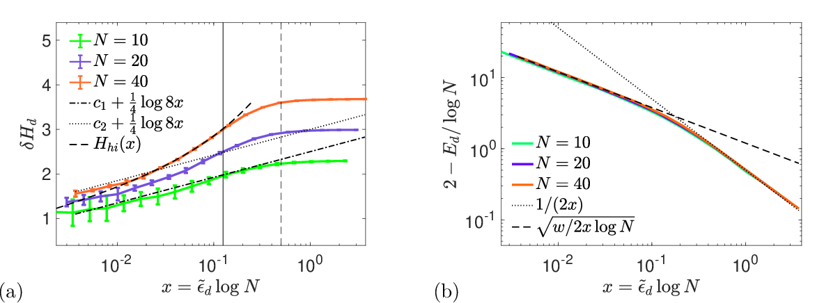
The asymptotic entropy rate would be obtained from \(\lim_{\ell \to \infty} H_d(\ell)\). Note however that \(F(L) \sim \log L \sim \log \log \ell\) as \(\ell \to \infty\), so in fact Eq.@eq:Hd predicts that the entropy rate is never attained. This is an artifact of the semi-annealed approximation, since at large enough \(G\) the semi-annealed saddle becomes unphysical. However this dependence is so slow that it is not a problem in practice. For example at \(G=10^{12}\) we have \(\log \log G - \frac{2}{\log \log G} - \log \log \log G \approx 1.5\). Hence we can consider a convenient renormalization scale \(\ell_\infty\) to define the entropy rate. Ignoring the slow factors we get \[\begin{align} \label{Hd2} H_d(\ell_\infty) \approx \frac{1}{4} \log 8x + \text{const} \qquad x\ll 1/8 \end{align}\tag{26}\] As shown in Fig.7a in the dotted and dash-dotted lines, this correctly predicts the logarithmic behavior in the frozen regime, with the correct prefactor \(1/4\).

Later we will use the finite-\(\ell\) dependence. The leading term gives \[\begin{align} \label{Hd3} H_d(\ell) - H_d(\ell_\infty) \approx \text{const} - \frac{1}{2}\log \alpha \qquad x\ll 1/8 \end{align}\tag{27}\]

Although not accessed in our numerics, theory predicts a crossover to a very low-temperature saturation regime at \(x<x_{lo}\) where \(H_d\) asymptotes.

7.1.2 Entropy in the critical region:↩︎

For \(x<1/8\) but close to \(1/8\) we obtain another contribution from the singularity at \(x=1/8\). We have \[\begin{align} \log z & = - \log a - \frac{3}{k_* - a } + \ldots \end{align}\] with \(k_* \approx \frac{3}{4} + \frac{1}{2}a + \frac{1}{2}\sqrt{a^2 + a + \frac{9}{4}}\). Then we get (with \(a \sim \sqrt{8x}/\beta\)) \[\begin{align} \label{Hc} H_d(\ell_\infty) \approx \frac{1}{4} \log 8x + \frac{3k_*/2}{(k_*-\sqrt{8x})^2} + \text{const} \qquad x \approx 1/8 \end{align}\tag{28}\] Call this prediction \(H_{hi}(x)\). It predicts the observed steepening of \(H_d\) as \(x \to 1/8^-\), as shown in Fig.7a (dashed curve).

7.1.3 Entropy in the transition region:↩︎

In the transition regime we need both \(\log z\) and the \(p/n\) terms. We have, in the scaling limit, \(-\log z + (p/n)\log(e/v) = 1 + \chi \log N + \ldots\) so that \[\begin{align} H_d(\ell_\infty) & \approx \left(1 - \frac{1}{8x} \right) \log N + \frac{1}{2} \qquad 1/8<x<1/2 \end{align}\] independent of \(\ell_\infty\) in this approximation.

This result is very interesting as it implies a change of scaling \(H_d \sim \log N\) for \(x>1/8\) to \(H_d \sim 1\) for \(x<1/8\). This is visible in Fig.7a, and in plots of normalized entropy, e.g. Fig. 2 of [17]. In the scaling limit it implies that \(x\approx 1/2\) is where we will first see the entropy drop from its maximal value, although for large enough \(N\) it will be \(\mathcal{O}(\log N)\) until \(x=1/8\).

7.2 Energy:↩︎

We likewise obtain results for the energy. We restrict to the hidden part of energy, \(E_d\), which is obtained from the part of \(\log Z\) proportional to \(\ell-m\). This leads to \[\begin{align} \langle E_d \rangle & = - \left.\frac{\partial}{\partial\beta}\right|_{\beta=1} \left[ \beta \log \bar M + \tilde{n}(\beta) + \frac{p}{\ell-m} \log e/v \right] \notag\\ & = \log N^2 - \begin{cases} \frac{1}{2\tilde{\epsilon}_d} & x \gtrsim 1/8 \\ \sqrt{\frac{w}{2\tilde{\epsilon}_d}} + \ldots& x < 1/8 \end{cases} , \end{align}\] where we neglect subleading terms. In the frozen regime the leading term is \(2 - \langle E_d \rangle/\log N = \sqrt{w/ 2\tilde{\epsilon}_d\log^2 N} \approx \sqrt{2/x}\). Note that the two regimes match at \(2 w \tilde{\epsilon}_d= 1\) which reduces to \(x = 1/8 + \tilde{\epsilon}_d/4 \log (\pi/\tilde{\epsilon}_d)\); in the scaling limit this becomes \(x=1/8\) as expected. Hence \(\langle E_d \rangle\) is continuous in the semi-annealed approximation, and clearly shows the phase transition at \(x_c=1/8\).

The theoretical predictions are compared with numerics in Fig.7b. They are quantitatively good, only entailing a small error near the transition point.

8 Application to natural language↩︎

The relations \(p \sim (\ell-m)^\beta\) and \(q \sim \ell^{\beta'}\) for the number of unique hidden and lexical rules in a corpus of total length \(\ell\) are related to a known linguistic law called Heaps law [2]. The latter states that the number of unique words in a corpus of length \(\ell\) satisfies \(n_* \sim \ell^b\) where \(b \approx 1/2\). The two laws are not identical, because we can have multiple rules \(a \to B\) for different hidden symbols \(a\) that yield the same word \(B\). However since the rules are iid in the RLM, we can derive the needed law.

Indeed, a word \(B\) appears in a corpus if and only if at least one lexical rule yields \(B\). Since the words are uniform, the probability that \(B\) doesn’t appear is \((1-1/T)^q\). Then the expected number of unique words is \[\begin{align} \label{Heaps} n_* = T \left( 1 - \left(1-\frac{1}{T} \right)^q \right) \approx T (1 - e^{-q/T} ) \end{align}\tag{29}\] where the latter expression holds if \(q \lesssim T\). Thus if \(q \sim \ell^{\beta'}\) then we predict \(n_* \sim \ell^{\beta'}\) for \(q \ll T\), which is exactly Heaps law. Moreover, we predict \(\beta' = 1/2\) near \(y=1/4\), which is exactly the most typically reported value.

A detailed analysis on large texts [6] found values \(b = 0.54, 0.52, 0.60, 0.47,\) and \(0.51\) for English, French, German, Hebrew, and Spanish, respectively. Two languages, Chinese and Russian, showed a two-regime law, with \(b = 0.77\) and \(b=0.65\) when fit to a single power law. The empirical results are in quite remarkable agreement with the theory. Above we found that in the transition region we have approximately \(\beta = 0.5\), while \(\beta = 0.53..\) near the critical point \(x=1/8\), and that \(\beta\) (and likewise for \(\beta'\)) will gradually decrease as \(x\) (\(y\)) decreases. Note that the predictions for \(\beta'\) are identical in the corresponding regime. Thus the data supports that languages are not far from the freezing transition at \(x=1/8, y=1/4\).

The prediction Eq.@eq:Heaps actually implies a saturation of Heaps law as \(q \to T\), i.e. when the corpus exhausts the vocabulary. The approach of saturation is visible in the plots of [6].

Heaps law is related to Zipf’s law [1], [36], the power-law relationship between the frequency of a word \(f_B\) and its rank, \(r_B\), with \(f_B \propto r_B^{-\zeta}\) and \(\zeta \approx 1\). This relationship can be expressed in terms of the probability of a word frequency \(f\), \(\mathbb{P}(f) \sim f^{-\alpha}\). Asymptotically \(\alpha = 1 + 1/\zeta\) [7], but it was noted in [7] that \(\mathbb{P}(f)\) generally shows two regimes with distinct exponents \(\alpha_\pm\), \(\mathbb{P}(f) \sim f^{-\alpha_-}\) for \(f < f_*\) and \(\mathbb{P}(f) \sim f^{-\alpha_+}\) for \(f > f_*\) . In this case \(\alpha_+ = 1+1/\zeta\) but no simple relation holds for \(\alpha_-\). In the absence of two-regime scaling, \(b=1/\zeta\).

In principle it should be possible to extract a \(\mathbb{P}(f)\) from the theory, but it does not appear straightforward. It was shown empirically in [17] that a two-regime Zipf law is reproduced by the RLM.

Heaps’ law can also be rationalized by a sample-space-reducing model in which the number of accessible states decreases as a text is written [37], [38]. Such models, however, fail to match the observed correlation structure between words. This structure is captured implicitly by the dependence of entropy on text length, to which we turn next.

9 Application to Large Language Models↩︎

9.1 Dependence of entropy on context length↩︎

Recently, Ref.[40] measured the code length \(\mathcal{L} = -\langle \log P(x_0 | x_{-K},x_{-K+1},\ldots x_{-1}) \rangle\) of natural language, as a function of context length \(K\). \(\mathcal{L}\) is a proxy for the entropy rate over text blocks of length \(K\), and it has the same behavior over different datasets and models [40]. In all cases it was observed that \(\mathcal{L}\) decreases approximately logarithmically with \(K\); see the red curve in Fig.8 for an example, measured from OLMo 2 [39], a Large Language Model with \(10^9\) parameters.

We model these results as follows: since grammar-based codes are universal [18], we can model any source as a stochastic context-free grammar, and thus place any source in the RLM phase diagram. We obtain a prediction for \(\mathcal{L}\) by assuming that tokens are in one-to-one correspondence with hidden symbols, and that the surface layer is a deterministic map, as discussed above. Since we expect the number of hidden symbols to be very large, and the entropy rate of natural language is finite, we expect the data to be in the frozen regime. Then from Eq.@eq:Hd3 , we obtain \[\begin{align} \mathcal{L}(K) = \text{const} - \frac{1}{2}\log \alpha + \ldots \end{align}\] in nats/token, where \(\alpha(G) = e^{-W_{-1}(-1/\log G^{2/3})} \approx \log G^{2/3} \log \log G^{2/3}\) and we have \(G = K/Na\) since \(K\) plays the role of corpus length. To convert to an entropy rate in bits/character we multiply by \(1/(n_{c/t}\log 2)\) where \(n_{c/t}=4.79\) is the number of characters per token in this dataset [40]. This expression is only expected to hold for large enough \(G\). The theoretical expression has two fitting parameters: the additive constant, and the product \(Na\). With \(Na \approx 2.2\) we obtain a good fit (Fig.8, blue curve) over the entire range that the solution exists, that is \(G \gtrsim 59\).

10 Conclusion↩︎

In this work we have developed a controlled theory of the Random Language Model in a (double) scaling limit where the grammar temperature \(\tilde{\epsilon}_d\to 0\) and the number of hidden symbols \(N\to \infty\) at fixed \(x = \tilde{\epsilon}_d\log N\). In this limit, the model exhibits a condensation transition at \(x_c=1/8\), inherited from the Random Energy Model, and governed by the breakdown of the law of large numbers in sums over grammar weights. This resolves the apparent paradox between finite-\(N\) numerical results, which show smooth crossover behavior, and the existence of a sharp transition in the thermodynamic limit. We focus on the regime of a large corpus, \(G \gg 1\) where \(G \sim n/N\sqrt{8x}\) is a rescaled corpus length that emerges from the theory.

The key technical step is the reorganization of the partition function as a sum over patterns, characterized by their rule multiplicity spectrum \(\{ p_k, q_k \}\). This leads to a semi-annealed description in which the dominant contribution arises from a saddle-point pattern. Within this framework, the number of distinct rules \(p\), or equivalently the ratio \(p/N\), emerges as a natural order parameter. In the high-temperature (“babbling") regime, weight is distributed over many rules and \(p/N \sim G\), corresponding to delocalized grammar usage and high entropy. In contrast, below \(x_c\) the model enters a frozen phase in which weight condenses onto a small subset of rules, \(p/N \sim G^{\beta(G)}\) where \(\beta(G) < 1\) is nontrivial, leading to low entropy and strongly constrained structure. The transition between these regimes is continuous in finite systems but sharp in the scaling limit.

The semi-annealed theory provides explicit predictions for the rule spectrum, entropy, and energy, and explains the scaling of the number of distinct rules with corpus size and temperature. In particular, it rationalizes the emergence of Heaps’ law and its continuously varying exponent as a function of \(x\), and connects these behaviors to the proximity of the system to the condensation transition. More generally, the theory shows how coarse-grained statistical regularities of language can arise from an ensemble of generative grammars through a well-defined statistical-mechanical mechanism.

The framework also provides a natural interpretation of recent observations in large language models. Retaining the corpus-length dependence of entropy (or code length) in the theory, we capture empirical measurements over several orders of magnitude in context length.

Several directions remain open. A more complete treatment of the quenched problem, beyond the semi-annealed approximation, would further clarify the nature of fluctuations around the saddle-point pattern. It would also be of interest to extend the analysis to richer grammatical structures beyond context-free rules [41], [42], and to connect the present static theory to dynamical or learning-based formulations, in which the parameters \(x\) and \(N\) emerge from training processes. Similarly, although the present results suggest that many features of natural language are captured by the purely random ensemble, it would be useful to incorporate grammatical parameters, and their known phylogenetic relations, into the theory [43]–[45].

More broadly, our results suggest that universal statistical properties of language may be understood as consequences of an underlying condensation transition in the space of generative models.

Finally, the semi-annealed construction is not specific to language, but applies more broadly to systems in which macroscopic behavior is controlled by rare configurations selected from a disordered ensemble. Examples include glasses [46], optimization landscapes in machine learning, random Markov systems [47], [48], random growth processes [49], and evolutionary fitness landscapes, where dominant states arise from extreme-value statistics but must be described in terms of coarse-grained, permutation-invariant observables.
Acknowledgments: EDG acknowledges conversations with Alessio Giorlandino, Sebastian Goldt, and Alessandro Treves, and NSERC Discovery Grant RGPIN-2020-04762.

References↩︎

---

1. \(Z_{tree} = 2p_E/(1+|2p_E-1|) = 1\) for \(p_E>1/2\).↩︎

2. The idea to relate belief propagation equations to the Random Energy Model is due to Alessio Giorlandino and Sebastian Goldt.↩︎

3. Here we have fixed a typo in the second and fourth equations, with \(H_{a'}\) rather than \(H_a\) as published in [19].↩︎

4. This procedure does not strictly enforce that each pile has exactly \(\ell_c\) rules, counted with multiplicity. However in the large \(m_c\) limit this is the most likely outcome. The corrections are computable; see Appendix 12 on Contingency Tables.↩︎

5. We have \(g^2 \approx 1/8\) to get large trees↩︎