A Structure-Preserving Neural-Spectral Method for Reconstructing Controls of Wave Equations
January 01, 1970
Abstract
The numerical reconstruction of controls for partial differential equations remains comparatively underdeveloped, despite the extensive analytical literature on controllability. This difficulty is particularly pronounced for wave equations, whose conservative structure, oscillatory dynamics, and high-frequency behavior make direct discretization and optimization challenging. In this work, we introduce a Neural-Spectral method for approximating controls of wave equations. The method represents both the state and the control in a Dirichlet spectral basis and parameterizes the time-dependent modal coefficients using shallow neural networks. In this way, the spatial oscillatory structure of the wave equation is built into the approximation, and the learning task is reduced to reconstructing temporal coefficients. We prove approximation results showing that, under the standing assumption that an exact control exists in the relevant energy framework, the control-state pairs found can approximate exact controlled trajectories uniformly in time in the energy norm, while also approximating the corresponding controls in \(L^2\). We also state a conditional computable error estimate that separates spectral truncation, neural-network approximation, quadrature, and optimization errors. In addition, we discuss structural obstructions faced by standard time-stepping schemes for conservative wave dynamics: explicit Euler amplifies high frequencies, implicit Euler introduces artificial dissipation, and Crank–Nicolson preserves amplitudes but compresses high-frequency phases. Numerical experiments in one, two, and three space dimensions illustrate the method on nonlinear, linear-reference, and high-dimensional control benchmarks. In a strongly nonlinear one-dimensional test, a Galerkin–Schauder HUM fixed-point implementation is observed to lose convergence for the parameter regime considered, while the Neural-Spectral method produces a forward-validated steering control. In two dimensions, we compare the method with a standard soft-constrained PINN on a GCC-compatible boundary-collar actuator, and we also include a linear Gramian reference benchmark in which the exact finite-dimensional minimum-energy control can be computed. This additional test shows that, when a classical Galerkin HUM reference is available, the Neural-Spectral formulation can recover a control close to the Gramian control and achieve small forward-validation terminal error. In three dimensions, the method is compared with a DeepONet-based forward surrogate. In the reported tests, the Neural-Spectral method attains smaller forward-validation terminal errors than these particular baselines. These results suggest that incorporating the spectral structure of the wave equation into the learning architecture can improve control reconstruction accuracy in the tested regimes. The DeepONet comparison also illustrates a complementary trade-off: the Neural-Spectral method is optimized separately for each control instance, whereas DeepONet can provide faster inference once its offline training cost has been amortized.
1 Introduction↩︎
The control theory of partial differential equations has been the subject of sustained and intensive investigation over the last several decades. For wave, heat, and dispersive equations, a large body of work has established exact, null, and approximate controllability via internal and boundary controls under a variety of geometric, analytic, and structural hypotheses; see, for instance, [1]–[4] and the references therein. In the case of wave equations, the Geometric Control Condition (GCC) plays a central role: in multidimensional domains, exact controllability is closely tied to the requirement that every generalized ray of geometric optics enters the control region within the prescribed time interval [5].
By contrast, the numerical reconstruction of controls remains much less developed. Even when controllability is established at the analytical level, it is often difficult to compute a reliable control that steers the system between prescribed states. Nonlinearities may also introduce loss of compactness, nonconvexity, stiffness, and instability in the numerical reconstruction procedure. Thus, while the existence of controls is well understood in many settings, the design of stable, accurate, and computationally tractable methods for approximating such controls remains a challenging and comparatively underdeveloped area.
A number of recent works have begun to address this issue from a constructive and numerical perspective. Least-squares, space-time, and fixed-point approaches have been developed for partial differential equations, including distributed and boundary control problems; see, for example, [6]–[10]. These works show that numerical control reconstruction is a subtle problem even in low dimensions. In higher dimensions, the difficulty is compounded by the cost of mesh-based discretizations and by the need to resolve interactions among the control region, high-frequency modes, and the conservative structure of the equations.
Machine learning provides a natural complementary set of tools for this problem, although most existing scientific machine learning methods were not designed specifically for control reconstruction. Physics-informed neural networks (PINNs), introduced in [11]–[13], approximate solutions of differential equations by training neural networks against PDE residuals, boundary conditions, and available data. PINNs have become a central tool in scientific machine learning for forward and inverse PDE problems, especially in data-sparse settings. However, the direct reconstruction of controls is a fundamentally different task: the control is an unknown input that must be chosen so that the corresponding state satisfies terminal steering constraints. Thus, the control problem imposes constraints not only on the state equation but also on the mechanism by which the unknown input enters the dynamics.
Several PINN variants have been proposed to address optimization difficulties, gradient flow stiffness, spectral bias, and gradient imbalance among different loss components; see, for example, [14]–[21]. These developments substantially improve the performance of PINNs for many forward and inverse problems. Nevertheless, they do not by themselves resolve the particular difficulty of control reconstruction, where one must recover an admissible control that steers the PDE dynamics to a prescribed terminal state and whose effect may be localized, bilinear, or strongly coupled to the state. For connections between Control Theory and Machine Learning, we refer to the discussions in [22].
In the work [23], the authors introduced WeightedPINN, an operator-decomposed PINN framework designed specifically for the numerical reconstruction of controls in nonlinear PDEs. The main idea of WeightedPINN is to assign separate adaptive weights to the different components of the controlled PDE residual, such as the time derivative, spatial differential operators, nonlinear response, and control term, as well as to the boundary, initial, and terminal constraints. This produces a control-aware residual metric that is better adapted to gradient imbalance at the operator level and to the mechanism through which the unknown control enters the equation. In this sense, WeightedPINN represents a viable attempt to adapt the PINN methodology to the control-reconstruction setting.
The present paper develops a different approach. Rather than modifying the space-time PINN loss, we exploit the spectral structure of the wave equation. The wave operator is skew-adjoint in the energy space, and its spectrum is purely imaginary. On rectangular domains, the corresponding Dirichlet eigenfunctions provide an explicit orthonormal modal basis. We use this structure to reduce the control reconstruction problem to the learning of time-dependent spectral coefficients. Both the state and the control are represented as finite sums of spatial eigenfunctions, while the modal coefficients are parameterized by one-dimensional neural networks in time. We call this a Neural-Spectral method.
This spectral viewpoint is especially natural for wave equations. The conservative dynamics are encoded mode by mode, and the projected controlled equation becomes a system of forced oscillators. The unknown control enters through the modal forcing coefficients, or, in the case of a localized actuator, through the corresponding actuator overlap matrix. Thus, the method does not ask a neural network to rediscover the spatial oscillatory structure of the wave equation. Instead, the spatial structure is built into the approximation, and the learning task is reduced to reconstructing the temporal coefficients that steer the retained modes.
The purpose of this paper is to develop and analyze a structure-preserving neural approximation framework for wave equation control reconstruction. The method is designed to exploit the modal structure of the wave equation and to provide a computationally useful control ansatz whose training loss is directly aligned with the projected controlled dynamics.
The main contributions of the paper are as follows.
We formulate a Neural-Spectral framework for approximating controls of wave equations. The method represents the state and the control in the Dirichlet spectral basis and parameterizes the resulting temporal modal coefficients by shallow neural networks.
We prove approximation results for the Neural-Spectral method. Under the standing assumption that an exact control exists in the relevant energy framework, we show that the control can be approximated in \(L^2((0,T);\mathcal{E})\). We then prove residual and solution approximation estimates showing that exact controlled trajectories can be approximated uniformly in time, in the energy norm, by Neural-Spectral control-state pairs.
We state a conditional computable error estimate that separates the principal numerical error sources: spectral truncation, neural-network approximation, quadrature or collocation error, and optimization error. This estimate is not a global convergence theorem for the nonconvex optimizer, but it clarifies how the computable training loss relates to the forward-validation error.
We identify a structural obstruction faced by standard time-stepping schemes for wave equations. Explicit Euler produces spurious amplification, implicit Euler introduces artificial dissipation, and Crank–Nicolson, although energy-preserving, compresses high-frequency phases and fails to converge to the continuous unitary wave group in the operator norm. This motivates a formulation that works directly at the level of spectral coefficients rather than relying on a direct time-stepping discretization of the full PDE.
We provide numerical experiments in one, two, and three space dimensions. In one dimension, we test a strongly nonlinear semilinear wave equation and compare with a Galerkin–Schauder HUM fixed-point implementation. In the reported strongly nonlinear regime, this HUM-S iteration does not converge, while the Neural-Spectral method produces a forward-validated steering control. In two dimensions, we compare against a standard soft-constrained PINN on a GCC-compatible boundary-collar actuator. We also add a linear Gramian reference benchmark, where the finite-dimensional minimum-energy Galerkin control is computed explicitly and used as a classical reference solution. This benchmark verifies that the Neural-Spectral formulation can recover a control close to the Galerkin HUM control in a setting where an exact finite-dimensional reference is available. In three dimensions, we compare against a DeepONet forward surrogate combined with gradient-based control inversion. In all cases, the recovered controls are evaluated by independent forward simulation of the projected dynamics, rather than only by the training loss.
The numerical results illustrate the distinction between the present method and several natural computational baselines. In the one-dimensional strongly nonlinear test, a Galerkin–Schauder HUM fixed-point implementation loses its effective contraction property: the iterates fail to stabilize, and the resulting control does not steer the nonlinear semi-discrete dynamics accurately. By contrast, the Neural-Spectral method directly minimizes the projected residual and endpoint mismatch over a joint state-control parameterization; in the reported test, the training converges, and the recovered control gives a small forward-validation terminal error. This comparison should not be interpreted as a failure of HUM theory itself, but rather as evidence that the fixed-point implementation can become ineffective in strongly nonlinear regimes where a residual-based Neural-Spectral optimization remains useful. In the two-dimensional comparison, the PINN is trained with PDE, boundary, initial, and terminal penalties in the physical variables \((t,x,y)\). For the architecture, weighting, and optimization schedule used in this benchmark, the recovered PINN control has small amplitude and the forward-simulation terminal error remains close to the free-evolution baseline. The Neural-Spectral method, by contrast, optimizes the projected modal dynamics used in the validation step and gives a smaller terminal error on this test. This comparison highlights the potential advantage of aligning the training loss with the finite-dimensional controlled dynamics, while leaving open the possibility that more specialized PINN variants or different penalty strategies could improve the PINN baseline. In the three-dimensional comparison, the DeepONet experiment illustrates a cost–accuracy trade-off between per-instance optimization and amortized operator learning. The Neural-Spectral method is trained separately for each control problem and gives smaller forward-validated terminal errors on the two reported tests. DeepONet, on the other hand, shifts part of the computational cost to an offline training phase and therefore provides faster online inversion once the surrogate has been trained. The comparison should therefore be interpreted as evidence that the proposed method can provide higher per-instance accuracy in the tested setting, whereas operator-learning approaches may be preferable in many-query regimes where rapid online evaluation is more important than solving a single instance as accurately as possible.
The additional two-dimensional linear Gramian benchmark complements these comparisons by providing a classical non-machine-learning reference. In that test, the exact minimum-energy control of the projected Galerkin system is computed from the controllability Gramian, and the Neural-Spectral reconstruction is compared directly against this reference control. The results show close agreement with the Gramian/HUM control and small forward-validation terminal error. This benchmark should be viewed as a consistency check for the spectral control formulation in a setting where the finite-dimensional reference solution is available, rather than as a general superiority claim over all possible control solvers.
The paper is organized as follows. Section 2.1 introduces the controlled wave equation, the energy formulation, the spectral decomposition, and the Neural-Spectral ansatz. We then prove the control, residual, and solution approximation results in Section 2.2. Section 2.3 states the computable conditional error estimate. Section 3 discusses the obstruction created by standard time-stepping schemes for conservative wave dynamics. Finally, Section 4 presents the numerical experiments: a strongly nonlinear one-dimensional test, a two-dimensional comparison with a standard PINN, a two-dimensional linear Gramian reference benchmark, and a three-dimensional comparison with a DeepONet forward surrogate.
2 Controlling Wave Equations↩︎
2.1 The Neural-Spectral framework↩︎
Let \(\Omega=(0,1)^N\), and let \(\omega\subset \Omega\) be a nonempty open subset. For a given final time \(T>0\), we consider the following controlled wave equation with homogeneous Dirichlet boundary conditions: \[\label{Wave1} \begin{cases} \partial_{tt}{u} - \Delta u + g(u) + \alpha u + f\,\mathbf{1}_{\omega} = 0 & \text{in } (0,T)\times \Omega, \\[1mm] u(t,x) = 0 & \text{on } (0,T)\times \partial\Omega, \\[1mm] u(0,\cdot) = u^0,\quad \partial_t{u}(0,\cdot) = u^1 & \text{in } \Omega . \end{cases}\tag{1}\]
Here, \(u=u(t,x)\) denotes the state variable, and \(f=f(t,x)\) is an interior control acting on the subdomain \(\omega\), with \(\mathbf{1}_{\omega}\) denoting the characteristic function of \(\omega\). The constant \(\alpha \ge 0\) is real, and \(g:\mathbb{R}\to\mathbb{R}\) represents a nonlinear term. Subscripts in time denote differentiation with respect to \(t\). The objective is to construct an interior control \(f\), supported in \(\omega\), that steers the solution from the prescribed initial state \((u^0,u^1)\) to the prescribed terminal state \((u_T^0,u_T^1)\).
Remark 1. The function \(g:\mathbb{R}\to\mathbb{R}\) induces a Nemytskii operator on the relevant function spaces, \(u(\cdot,t) \in H_0^1(\Omega) \mapsto g\left(u(\cdot,t)\right) \in L^2(\Omega)\). By a slight abuse of notation, when there is no risk of confusion, we shall not distinguish between the scalar function and its induced operator, denoting both by \(g\).
Control problem. Given initial data \(\left(u^0,u^1\right)\) and target data \(\left(u_T^0,u_T^1\right)\), find a control \(f\) such that \[\label{Wave2} u(T,\cdot) = u_T^0, \qquad \partial_t{u}(T,\cdot) = u_T^1 \quad \text{in } \Omega .\tag{2}\]
According to [24], under the assumption that \(\omega\) satisfies appropriate geometric conditions (e.g., being a neighborhood of a suitable part of the boundary) and \(T\) is sufficiently large, if the nonlinearity \(g\) is globally Lipschitz or satisfies an appropriate growth condition at infinity (e.g., \(\lim\limits_{|s|\to\infty} \dfrac{|g(s)|}{|s|\log^2|s|} = 0\) [25]), the system 1 is exactly controllable. That is, for any initial data \[\left(u^0,u^1\right)\in H_0^1(\Omega)\times L^2(\Omega)\] and any target data \[\left(u_T^0,u_T^1\right)\in H_0^1(\Omega)\times L^2(\Omega),\] there exists a control \(f\) such that 2 holds.
Remark 2. Regarding the existence and regularity of the exact control \(f\), a sharp analytical distinction must be made between one-dimensional and multi-dimensional domains:
For the one-dimensional case (\(N=1\)), it has been rigorously proven that exact internal controllability holds with a control \(f \in L^2((0,T) \times \omega)\), provided the nonlinearity \(g(u)\) satisfies the critical logarithmic growth condition at infinity [25].
However, in multi-dimensional spaces (\(N \ge 2\)), achieving exact controllability for the semi-linear wave equation with strictly \(L^2\)-controls remains an open problem. As explicitly noted in [24], for globally Lipschitz nonlinearities, current fixed-point techniques only guarantee the existence of a control \(f \in H^{-\varepsilon}((0,T); L^2(\omega))\) for arbitrarily small \(\varepsilon > 0\) (specifically \(\varepsilon \in (0, 1/2)\)). The existence of a control strictly belonging to \(L^2((0,T) \times \omega)\) is not yet mathematically established in higher dimensions.
Although this leaves a theoretical gap in higher dimensions, the fact that \(H^{-\varepsilon}((0,T);L^2(\omega))\) is only slightly weaker than \(L^2((0,T)\times\omega)\), together with the constructive \(L^2\)-controllability results available in one dimension (see [25]), motivates the following standing assumption for the numerical part of the paper: \[f\in L^2((0,T)\times\omega).\]
Remark 3 (Geometric Control Condition). It is important to emphasize that the assumption of exact controllability for the multidimensional wave equation is intrinsically tied to the Geometric Control Condition (GCC). In the one-dimensional case (\(N=1\)), the exact controllability holds for any non-empty open subset \(\omega\) provided that \(T\) is sufficiently large. For instance, if \(\Omega = (0,1)\) and \(\omega = (l_1, l_2) \subset (0,1)\), the sharp condition is \(T > 2\max\{l_1, 1 - l_2\}\) [25]. However, the multi-dimensional framework (\(N \ge 2\)) strictly requires the pair \((\omega, T)\) to satisfy the Geometric Control Condition (GCC). Introduced in [5], the GCC states that every optical ray propagating in \(\Omega\) and reflecting on its boundary \(\partial\Omega\) must enter the control region \(\omega\) within the time interval \((0,T)\). As demonstrated by Bardos et al. [5], if there exists a generalized ray that never encounters the control region \(\omega\) within time \(T\) (a so-called "trapped ray"), the exact controllability to all states in the energy space cannot be achieved. Therefore, throughout this paper, we assume that \((\omega,T)\) satisfies the GCC.
Introducing the auxiliary variable \(z = \partial_t{u}\), system 1 can be rewritten as the first-order system \[\label{Wave3} \left\{ \begin{align} &u' = z, \\ &z' = \Delta u - \alpha u -g(u)- f\,\mathbf{1}_{\omega}, \\ &u(0) = u^0,\quad z(0) = u^1 . \end{align} \right.\tag{3}\]
Next, denoting \(\Phi = (u,z)\), \(G(\Phi) = (0,g(u))\), \(\mathbf{F} = (0,f)\), and \(\Phi_0=(u^0,u^1),\) and \(\Phi_T=(u^0_T,u^1_T),\) system 3 can be written in the abstract Cauchy form \[\label{Wave4} \left\{ \begin{align} &\Phi' + A\Phi + \mathbf{F}\,\mathbf{1}_{\omega} +G(\Phi) = 0, \\ &\Phi(0,\cdot) = \Phi_0,\;\;\; \Phi(T,\cdot) = \Phi_T . \end{align} \right.\tag{4}\]
We work in the energy space \[\mathcal{E}:=H_0^1(\Omega)\times L^2(\Omega),\] equipped with the inner product \[\left\langle (u_1,z_1),(u_2,z_2)\right\rangle_{\mathcal{E}} = \int_\Omega \left(\nabla u_1\cdot \overline{\nabla u_2} +\alpha u_1\overline{u_2}\right)\,dx + \int_\Omega z_1\overline{z_2}\,dx .\] Throughout this section, complex Hilbert inner products are taken to be linear in the first argument and conjugate-linear in the second. We define the operator \(A:D(A)\subset \mathcal{E}\to \mathcal{E}\) by \[D(A):=\left(H^2(\Omega)\cap H_0^1(\Omega)\right)\times H_0^1(\Omega),\] and \[A(u,z):= \begin{pmatrix} -z\\ -\Delta u+\alpha u \end{pmatrix}.\] With this realization, \(A\) is skew-adjoint on \(\mathcal{E}\) (see [26]).
Lemma 1 (Spectrum of \(A\)). The operator \(A\) has a purely imaginary point spectrum. For each multi-index \(k = (k_1, \dots, k_N) \in (\mathbb{N}^*)^N\), the eigenvalues of \(A\) and the associated normalized eigenfunctions are given by \[\begin{align} \lambda_k^\pm &= \pm \mathbf{i} \sqrt{\sum_{j=1}^N k_j^2 \pi^2 + \alpha}. \\ \phi_k^\pm(x) &= 2^{\frac{N-1}{2}} \begin{pmatrix} \dfrac{1}{\lambda_k^\pm} \medskip\\ -1 \end{pmatrix}^T \prod_{j=1}^N \sin(k_j \pi x_j), \quad x = (x_1, \dots, x_N) \in \Omega. \end{align}\] Moreover, the family \(\left\{ \phi_k^+, \phi_k^- \right\}_{k \in (\mathbb{N}^*)^N}\) forms an orthonormal basis of \(H_0^1(\Omega) \times L^2(\Omega)\).
Proof. To determine the eigenvalues of \(A\), we need to find \(\lambda \in \mathbb{C}\) such that the equation \(A\phi=\lambda\phi^T\) has at least one non-zero solution \(\phi=(u,z)\in H_0^1(\Omega) \times L^2(\Omega)\). From the definition of \(A\), this equation is equivalent to \[\left\{ \begin{align} &-z = \lambda u, \\ &-\Delta{u}+\alpha u = \lambda z. \end{align} \right.\] It implies that \[\label{Spectrum1} \left\{ \begin{align} &\Delta{u}=\left(\lambda^2+\alpha\right)u, \\ & u(x)=0 \text{ on } \partial\Omega. \end{align} \right.\tag{5}\] Note that \(\Omega=(0,1)^N\). Using the method of separation of variables on the open hypercube \(\Omega = (0,1)^N\), the eigenvalues of the Dirichlet Laplacian \(-\Delta\) are known to be \(\mu_k = \displaystyle\sum_{j=1}^N k_j^2\pi^2\) for \(k=(k_1,k_2,\ldots,k_N) \in (\mathbb{N}^*)^N\), with corresponding \(L^2\)-orthonormal eigenfunctions \(e_k(x) = 2^{\frac{N}{2}}\displaystyle\prod_{j=1}^N \sin(k_j \pi x_j)\). From 5 , we must have \(\lambda^2 + \alpha = - \mu_k\), which implies \(\lambda^2 = -(\mu_k + \alpha)\). Since \(\mu_k > 0\) and \(\alpha \ge 0\), we obtain two purely imaginary eigenvalues for each \(k \in (\mathbb{N}^*)^N\) as follows \[\lambda_k^\pm = \pm \mathbf{i} \sqrt{\mu_k + \alpha} = \pm \mathbf{i} \sqrt{\sum_{j=1}^N k_j^2\pi^2 + \alpha}.\] The corresponding eigenvectors of \(A\) take the form \(\phi_k^\pm(x) = C \begin{pmatrix} \dfrac{1}{\lambda_k^\pm} \medskip\\ -1 \end{pmatrix}^T e_k(x)\), where \(C\) is a complex normalization constant. Let us compute the norm of \(\phi_k^\pm\) in \(H_0^1(\Omega) \times L^2(\Omega)\). \[\left\|\phi_k^\pm\right\|_{H_0^1(\Omega) \times L^2(\Omega)}^2 = |C|^2 \left( \frac{1}{\left|\lambda_k^\pm\right|^2} \|e_k\|_{H_0^1(\Omega)}^2 + \|e_k\|_{L^2(\Omega)}^2 \right).\] By the definition of the norm on \(H_0^1(\Omega)\), using Green’s first identity, and taking into account that \(e_k|_{\partial\Omega} = 0\), we have \[\begin{align} \|e_k\|_{H_0^1(\Omega)}^2 = \int_\Omega |\nabla e_k|^2 dx + \alpha \int_\Omega |e_k|^2 dx = \int_\Omega (-\Delta e_k) e_k dx + \alpha \|e_k\|_{L^2(\Omega)}^2. \end{align}\] Since \(e_k\) is the eigenfunction of the Dirichlet Laplacian \(-\Delta\) associated with the eigenvalue \(\mu_k\), we have \(-\Delta e_k = \mu_k e_k\). Substituting this relation into the integral yields \[\label{H950941-norm-e95k} \|e_k\|_{H_0^1(\Omega)}^2 = \mu_k \int_\Omega |e_k|^2 dx + \alpha \|e_k\|_{L^2(\Omega)}^2 = (\mu_k + \alpha) \|e_k\|_{L^2(\Omega)}^2=\left|\lambda_k^\pm\right|^2\|e_k\|_{L^2(\Omega)}^2=\left|\lambda_k^\pm\right|^2.\tag{6}\] Thus, \(\left\|\phi_k^\pm\right\|_{H_0^1(\Omega) \times L^2(\Omega)}^2 = 2|C|^2\). Setting \(\|\phi_k^\pm\|_{H_0^1(\Omega) \times L^2(\Omega)} = 1\) requires \(|C| = \dfrac{1}{\sqrt{2}}\). Choosing \(C = \dfrac{1}{\sqrt{2}}\) yields the normalized eigenfunctions \(\phi_k^\pm(x)\) as follows \[\phi_k^\pm(x) = \dfrac{1}{\sqrt{2}} \begin{pmatrix} \dfrac{1}{\lambda_k^\pm} \medskip\\ -1 \end{pmatrix}^T e_k(x) = 2^{\frac{N-1}{2}} \begin{pmatrix} \dfrac{1}{\lambda_k^\pm} \medskip\\ -1 \end{pmatrix}^T \prod_{j=1}^N \sin(k_j \pi x_j), \quad x = (x_1, \dots, x_N) \in \Omega.\] Next, we prove that this family is orthonormal. For \(k \neq l \in (\mathbb{N}^*)^N\), the orthogonality \(\langle \phi_k^p, \phi_l^q \rangle_{H_0^1(\Omega) \times L^2(\Omega)} = 0\) (for \(p, q \in \{+, -\}\)) follows immediately from the orthogonality of the trigonometric polynomials \(e_k\) and \(e_l\) in both \(L^2(\Omega)\) and \(H_0^1(\Omega)\). For the same mode \(k\) but opposite branches (\(+\) and \(-\)), we evaluate their inner product \[\begin{align} \langle \phi_k^+, \phi_k^- \rangle_{H_0^1(\Omega) \times L^2(\Omega)} &= \dfrac{1}{2} \left[ \left\langle \frac{1}{\lambda_k^+} e_k, \frac{1}{\lambda_k^-} e_k \right\rangle_{H_0^1(\Omega)} + \langle -e_k, -e_k \rangle_{L^2(\Omega)} \right] \nonumber \\ &= \dfrac{1}{2} \left[ \frac{1}{\lambda_k^+} \overline{\left(\frac{1}{\lambda_k^-}\right)} \|e_k\|_{H_0^1(\Omega)}^2 + \|e_k\|_{L^2(\Omega)}^2 \right]. \end{align}\] Since \(\lambda_k^- = \overline{\lambda_k^+}\), we have \(\overline{(1/\lambda_k^-)} = 1/\lambda_k^+\). Hence, the coefficient in the first term is \(1/\left(\lambda_k^+\right)^2\). Knowing that \(\left(\lambda_k^+\right)^2 = -(\mu_k + \alpha)\) and \(\|e_k\|_{H_0^1(\Omega)}^2 = (\mu_k + \alpha)\|e_k\|_{L^2(\Omega)}^2\), we obtain \[\langle \phi_k^+, \phi_k^- \rangle_{H_0^1(\Omega) \times L^2(\Omega)} = \dfrac{1}{2} \left[ - \|e_k\|_{L^2(\Omega)}^2 + \|e_k\|_{L^2(\Omega)}^2 \right] = 0.\] Thus, the family \(\left\{ \phi_k^+, \phi_k^- \right\}_{k \in (\mathbb{N}^*)^N}\) is orthonormal. Since \(A\) is skew-adjoint on \(\mathcal{E}\), the operator \(B:=iA\) is self-adjoint. Moreover, \(A^{-1}\), and therefore \(B^{-1}\), is compact, as a consequence of the compact embedding \(H_0^1(\Omega)\hookrightarrow L^2(\Omega)\) (see, e.g., [27]). Hence, \(B\) has compact resolvent. The spectral theorem for self-adjoint operators with compact resolvent [27] implies that their eigenfunctions form a complete orthonormal basis of \(\mathcal{E}\). Since the eigenfunctions of \(B\) and \(A\) coincide, the family \[\{\phi_k^+,\phi_k^-\}_{k\in(\mathbb{N}^*)^N}\] forms a complete orthonormal basis of \(H_0^1(\Omega)\times L^2(\Omega)\). ◻
To make the spectral representation compatible with neural operator learning frameworks, it is natural and convenient to represent the states using a one-dimensional sequence rather than a complex multi-index. We establish this rigorous transition in the following lemma. The proof of this lemma is presented in Appendix 5.
Lemma 2 (1D spectral re-indexing). There exists a bijection \(\kappa : \mathbb{N}^* \to (\mathbb{N}^*)^N \times \{+, -\}\) that systematically re-indexes the multi-dimensional eigenvalues \(\lambda_k^\pm\) and eigenfunctions \(\phi_k^\pm(x)\) obtained in Lemma 1 into one-dimensional sequences \((\lambda_n)_{n \in \mathbb{N}^*}\) and \((\phi_n)_{n \in \mathbb{N}^*}\).
Remark 4. The proof of Lemma 1 shows a direct correspondence between the spectrum of the first-order wave operator \(A\) on \(H_0^1(\Omega)\times L^2(\Omega)\) and the spectrum of the Dirichlet Laplacian \(-\Delta\) on \(L^2(\Omega)\). Indeed, each vector-valued eigenfunction \(\phi_k^\pm\in H_0^1(\Omega)\times L^2(\Omega)\) associated with the eigenvalue \(\lambda_k^\pm\) of \(A\) is obtained from the scalar Dirichlet eigenfunction \(e_k\) associated with the eigenvalue \(\mu_k\) through \[\lambda_k^\pm=\pm \mathbf{i}\sqrt{\mu_k+\alpha}, \qquad \phi_k^\pm(x) = \frac{1}{\sqrt2} \begin{pmatrix} \dfrac{1}{\lambda_k^\pm}\\[5mm] -1 \end{pmatrix}^T e_k(x), \qquad k\in(\mathbb{N}^*)^N.\] After re-indexing as in the proof of Lemma 2 (see Appendix 5), this relation becomes \[\begin{align} &\lambda_{2n-1}= \lambda_{q(n)}^+ = \mathbf{i}\sqrt{\mu_n+\alpha}, \qquad \qquad \qquad \qquad\;\;\lambda_{2n}= \lambda_{q(n)}^- = -\mathbf{i}\sqrt{\mu_n+\alpha} \\ &\phi_{2n-1} = \phi_{q(n)}^+= \frac{1}{\sqrt2} \begin{pmatrix} \dfrac{1}{\lambda_{2n-1}}\\[5mm] -1 \end{pmatrix}^T e_{n}(x), \qquad \phi_{2n} = \phi_{q(n)}^-= \frac{1}{\sqrt2} \begin{pmatrix} \dfrac{1}{\lambda_{2n}}\\[5mm] -1 \end{pmatrix}^T e_{n}(x), \qquad n\in\mathbb{N}^*, \end{align}\] where \(q\) is defined by 57 in Appendix 5. Here, to shorten the mathematical expressions, we have identified \[\mu_{n}:=\mu_{q(n)}, \qquad e_{n} := e_{q(n)}.\]
With the one-dimensional re-indexing \((\lambda_n)_{n\in\mathbb{N}^*}\), \((\phi_n)_{n\in\mathbb{N}^*}\) established above, we now formulate the learning problem. The key idea is to represent both the state \(\Phi\) and the control \(\mathbf{F}\,\mathbf{1}_{\omega}\) as finite linear combinations of eigenfunctions of \(A\), with time-dependent coefficients parameterized by neural networks. Specifically, for a truncation order \(P\), we project the problem onto the finite-dimensional subspace \[\label{Wave7} \mathscr{V}_P := \operatorname{span}\left\{\phi^+_{q(j)},\, \phi^-_{q(j)} : j = 1, \ldots, P\right\} = \operatorname{span}\left\{\phi_{2j-1},\, \phi_{2j} : j = 1, \ldots, P\right\} = \{\phi_i\}_{i=1}^{2P} .\tag{7}\] We seek an approximate solution of the form \(\widetilde{\Phi}_{\theta_a} = \left(\widetilde{u}_{\theta_a}, \partial_t\widetilde{u}_{\theta_a}\right)\), where \[\widetilde{u}_{\theta_a}(t,x) = \sum_{j=1}^{P} a_j(t;\theta_a)e_j(x).\] where \[a_j(t;\theta_a)=A_j^a\cdot \sigma\left(W_j^a t+B_j^a\right),\qquad A_j^a,W_j^a,B_j^a\in\mathbb{R}^{m_a}, \qquad j=1,\ldots,P.\] Similarly, we approximate the control \(\mathbf{F}\,\mathbf{1}_{\omega}=\left(0,f\,\mathbf{1}_\omega\right)\) by \(\widetilde{\mathbf{F}}_{\theta_c}\,\mathbf{1}_{\omega}=\left(0,\widetilde{f}_{\theta_c}\mathbf{1}_\omega\right)\), where \[\widetilde{f}_{\theta_c}(t,x) =\sum_{j=1}^{P} c_j(t;\theta_c)e_j(x),\] and \[c_j(t;\theta_c) = A_j^c\cdot \sigma\left(W_j^c t+B_j^c\right), \qquad A_j^c,W_j^c,B_j^c\in\mathbb{R}^{m_c}, \qquad j=1,\ldots,P.\] Here \(\sigma\) acts component-wise and “\(\cdot\)” denotes the Euclidean inner product. Thus \[\theta_a = \left(A_i^{a},W_i^{a},B_i^{a}\right)_{i=1}^{P} \in (\mathbb{R}^{m_a})^{3P}, \qquad \theta_c = \left(A_j^c,W_j^c,B_j^c\right)_{j=1}^{P} \in (\mathbb{R}^{m_c})^{3P}.\] The full parameter vector is then \[\theta=(\theta_a,\theta_c).\] Accordingly, the state and control approximations are written as \[\widetilde{\Phi}_{\theta_a}(t,x) = \sum_{j=1}^{P}{\left(a_j(t;\theta_a), a_j'(t;\theta_a)\right)e_j(x)},\] and \[\widetilde{\mathbf{F}}_{\theta_c}(t,x)\,\mathbf{1}_\omega(x) = \left(0,\,\mathbf{1}_\omega(x)\sum_{j=1}^{P} c_j(t;\theta_c)e_j(x)\right).\] Suppose that \(\widetilde{\Phi}_{\theta}(t,x) =\displaystyle\sum_{j=1}^{P}{\left(a_j(t;\theta_a), a_j'(t;\theta_a)\right)e_j(x)}\) is a solution of 4 projected onto \(\mathscr{V}_P\) and controlled by \(\widetilde{\mathbf{F}}_{\theta_c}\). Restricting the problem 4 to \(\mathscr{V}_P\), taking the \(\mathcal{E}\)-inner product of 4 with \(\phi_i\) and noting that \[\left\langle A\widetilde{\Phi}_{\theta}(t,\cdot), \phi_i \right\rangle = \left\langle \widetilde{\Phi}_{\theta}(t,\cdot), A^*\phi_i \right\rangle = \left\langle \widetilde{\Phi}_{\theta}(t,\cdot), -A\phi_i\right\rangle = \left\langle \widetilde{\Phi}_{\theta}(t,\cdot), -\lambda_i\phi_i\right\rangle = -\overline{\lambda_i}\left\langle \widetilde{\Phi}_{\theta}(t,\cdot), \phi_i \right\rangle,\] we arrive at \[\begin{align} \left\langle \widetilde{\Phi}'_{\theta}(t,\cdot), \phi_i\right\rangle +\lambda_i\left\langle \widetilde{\Phi}_{\theta}(t,\cdot), \phi_i \right\rangle + \left\langle G\left(\widetilde{\Phi}_{\theta}(t,\cdot)\right),\phi_i\right\rangle_{\mathcal{E}} + \left\langle\widetilde{\mathbf{F}}_{\theta_c}(t,\cdot),\phi_i\right\rangle_{\mathcal{E}}=0,\quad t \in (0,T),\quad i=1,\ldots, 2P. \end{align}\] Note that we have used \(\overline{\lambda_i}=-\lambda_i\), which follows from \(\lambda_i \in \mathbf{i}\mathbb{R}\). Moreover, observe that \[\begin{align} \left\langle \widetilde{\Phi}_{\theta}(t,\cdot), \phi_{2j-1} \right\rangle_{\mathcal{E}} = \dfrac{1}{\sqrt{2}}\left(\dfrac{a_j(t;\theta)}{\overline{\lambda_{2j-1}}}\|e_j\|^2_{H_0^1(\Omega)}-a_j'(t;\theta)\|e_j\|^2_{L^2(\Omega)}\right) = \dfrac{-1}{\sqrt{2}}\left(a_j'(t;\theta)-\mathbf{i}\sqrt{\mu_j+\alpha}\,a_j(t;\theta)\right) \tag{8}\\ \left\langle \widetilde{\Phi}_{\theta}(t,\cdot), \phi_{2j} \right\rangle_{\mathcal{E}} = \dfrac{1}{\sqrt{2}}\left(\dfrac{a_j(t;\theta)}{\overline{\lambda_{2j}}}\|e_j\|^2_{H_0^1(\Omega)}-a_j'(t;\theta)\|e_j\|^2_{L^2(\Omega)}\right) = \dfrac{-1}{\sqrt{2}}\left(a_j'(t;\theta)+\mathbf{i}\sqrt{\mu_j+\alpha}\,a_j(t;\theta)\right). \tag{9} \end{align}\] Furthermore, since \(G\left(\widetilde{\Phi}_{\theta}\right)=\left(0,g\left(\widetilde{u}_{\theta}\right)\right)\), \(\widetilde{\mathbf{F}}_{\theta_c}=\left(0,\widetilde{f}_{\theta_c}\right)\), we have
\[\begin{align} \left\langle G\left(\widetilde{\Phi}_{\theta}(t,\cdot)\right),\phi_{2j-1}\right\rangle_{\mathcal{E}} &= \left\langle G\left(\widetilde{\Phi}_{\theta}(t,\cdot)\right),\phi_{2j}\right\rangle_{\mathcal{E}}=\dfrac{-1}{\sqrt{2}}\left\langle g\left(\widetilde{u}_{\theta}(t,\cdot)\right),e_j\right\rangle_{L^2(\Omega)} \\ & = \dfrac{-1}{\sqrt{2}}\left\langle g\left(\sum_{\ell=1}^{P} a_\ell(t;\theta_a)e_\ell\right),e_j\right\rangle_{L^2(\Omega)} \end{align}\] and \[\begin{align} \left\langle\widetilde{\mathbf{F}}_{\theta_c}(t,\cdot)\,\mathbf{1}_\omega,\phi_{2j-1}\right\rangle_{\mathcal{E}}&=\left\langle\widetilde{\mathbf{F}}_{\theta_c}(t,\cdot)\,\mathbf{1}_\omega,\phi_{2j}\right\rangle_{\mathcal{E}}=\dfrac{-1}{\sqrt{2}}\left\langle\widetilde{f}_{\theta_c}(t,\cdot)\,\mathbf{1}_\omega,e_j\right\rangle_{L^2(\Omega)}\\ &=\dfrac{-1}{\sqrt{2}}\left\langle\mathbf{1}_\omega\,\sum_{\ell=1}^{P} c_\ell(t;\theta_c)e_\ell,e_j\right\rangle_{L^2(\Omega)}=\dfrac{-1}{\sqrt{2}}\sum_{\ell=1}^P M_{j\ell}\,c_\ell(t;\theta_c), \end{align}\] where \[M_{j\ell} = \int_\omega e_j(x)e_\ell(x)\,dx.\] Therefore, considering the two cases \(i=2j-1\) and \(i=2j\), we obtain the same system as follows \[\begin{align} \label{Wave8} a_j''(t;\theta)+(\mu_j+\alpha)a_j(t;\theta) +\left\langle g\left(\sum_{\ell=1}^{P} a_\ell(t;\theta)e_\ell\right),e_j\right\rangle_{L^2(\Omega)} +\sum_{\ell=1}^P M_{j\ell}\,c_\ell(t;\theta_c)=0,\notag\\ t \in (0,T),\,j=1,\ldots, P. \end{align}\tag{10}\]
However, since the neural network \(a_j(t;\theta)\) is determined by the parameters \(\theta\) rather than by solving 10 , the left-hand side of 10 does not vanish in general. For each \(t \in (0,T)\) and \(j=1,\ldots, P\), we define the residual \(R_j(t;\theta)\) as this remaining quantity \[\begin{align} \label{Wave9} &R_j(t;\theta)=a_j''(t;\theta)+(\mu_j+\alpha)a_j(t;\theta) +\left\langle g\left(\sum_{\ell=1}^{P} a_\ell(t;\theta)e_\ell\right),e_j\right\rangle_{L^2(\Omega)} +\sum_{\ell=1}^P M_{j\ell}\,c_\ell(t;\theta_c). \end{align}\tag{11}\] The goal is to find \(\theta\) such that \(R_j(t;\theta) \approx 0\) for all \(j=1,\ldots, P\) and the terminal condition \(\widetilde{\Phi}_\theta(T,\cdot) \approx \Phi_T\) is satisfied. This motivates us to minimize \[\label{Wave10} \min_\theta \left[ \sum_{j=1}^P \|R_j(\cdot;\theta)\|_{L^2(0,T)}^2 + \left\| \sum_{j=1}^P \left(a_j(0;\theta), a_j'(0;\theta)\right)e_j-\Phi_0 \right\|_{\mathcal{E}}^2 + \left\| \sum_{j=1}^P \left(a_j(T;\theta),a_j'(T;\theta)\right)e_j-\Phi_T \right\|_{\mathcal{E}}^2 \right].\tag{12}\]
A minimizer \(\theta^*\) of 12 simultaneously yields an approximate control \(\widetilde{\mathbf{F}}_{\theta^*}\) and an approximate solution \(\widetilde{\Phi}_{\theta^*}\).
2.2 Approximation results↩︎
Having established the Neural-Spectral formulation, we now turn to its theoretical guarantees. In this section, we prove that the proposed architecture possesses sufficient representational capacity to approximate exact control-state pairs. We begin by specifying the regularity requirements for the neural network activation function, which are essential for establishing the density of the approximation space.
Assumption 1. (Activation function)We assume that the scalar activation function \(\sigma:\mathbb{R}\to\mathbb{R}\) belongs to \(C^2(\mathbb{R})\) and is not a polynomial. For vector inputs, \(\sigma\) acts component-wise. This property is satisfied by standard smooth non-polynomial activations, such as \(\tanh\), sigmoid, softplus, Swish, and GELU.
Lemma 3. Let Assumption 1 hold. Then the class \[\mathcal{N}_\sigma := \left\{ \sum_{\ell=1}^m A_\ell \sigma(W_\ell t+B_\ell) : m\in\mathbb{N}^*,\; A_\ell,W_\ell,B_\ell\in\mathbb{R} \right\}\] is dense in \(W^{2,2}(0,T)\). Equivalently, for every \(a\in W^{2,2}(0,T)\) and every \(\varepsilon>0\), there exists \(a_\theta\in\mathcal{N}_\sigma\) such that \[\|a-a_\theta\|_{W^{2,2}(0,T)}<\varepsilon .\] Consequently, \(\mathcal{N}_\sigma\) is also dense in \(L^2(0,T)\).
Proof. We employ a two-step density argument as formulated by [28] for Sobolev spaces. Since the interval \((0, T)\) is bounded and possesses the segment property, by [29], the space of infinitely continuously differentiable functions \(C^\infty[0, T]\) is dense in \(W^{2,2}(0, T)\). Thus, there exists an auxiliary function \(v \in C^\infty[0,T]\) such that \[\label{lem8-est4-a} \| v - a \|_{W^{2,2}(0,T)} < \dfrac{\varepsilon}{2},\tag{13}\] Then, since \(v \in C^\infty[0, T] \subset C^2[0, T]\), by invoking [30], there exists a neural network \(a_{\theta} \in \mathcal{N}_\sigma\) that approximates \(v\) uniformly in \(C^2[0,T]\), with a sufficiently large width \(m\) and parameters \(\theta \in \left(\mathbb{R}^{m}\right)^{3P}\). Utilizing the inequality \(\| u \|_{W^{2,2}(0,T)} \le \sqrt{3T} \| u \|_{C^2[0,T]}\), we have \[\label{lem8-est5-a} \left\| a_{\theta} - v \right\|_{W^{2,2}(0,T)} \le \sqrt{3T} \left\| a_{\theta} - v\right\|_{C^2[0,T]} < \dfrac{\varepsilon}{2}.\tag{14}\] From 13 and 14 , we obtain \[\left\| a - a_\theta\right\|_{W^{2,2}(0,T)} \le \| a_{\theta} - v \|_{W^{2,2}(0,T)} + \| v - a\|_{W^{2,2}(0,T)} < \varepsilon,\] which demonstrates that \(\mathcal{N}_\sigma\) is dense in \(W^{2,2}(0,T)\). Consequently, since \(W^{2,2}(0,T) \hookrightarrow L^2(0,T)\) and \(W^{2,2}(0,T)\) is dense in \(L^2(0,T)\), \(\mathcal{N}_\sigma\) is also dense in \(L^2(0,T)\). ◻
Lemma 4 (Projection of the control). Let \(\Pi_P\) denote the orthogonal projection of \(\mathcal{E}:=H_0^1(\Omega)\times L^2(\Omega)\) onto \(\mathscr{V}_P\) (defined in 7 ), and let \(\pi_P\) denote the orthogonal projection of \(L^2(\Omega)\) onto \[E_P:=\operatorname{span}\{e_j\}_{j=1}^{P} \subset L^2(\Omega).\] If \(\mathbf{F}=(0,f)\), with \(f\in L^2((0,T)\times\omega)\), then, for a.e. \(t\in(0,T)\), \[\Pi_P\left(\mathbf{F}(t,\cdot)\right) = \left(0,\pi_P(f(t,\cdot))\right).\]
Proof. Since \(\{\phi_i\}_{i=1}^{2P}\) forms an orthonormal family in \(\mathcal{E}\) (see Lemma 1), \[\begin{align} \label{eq:proj95expand} \Pi_P\left(\mathbf{F}(t,\cdot))\right) &= \sum_{i=1}^{2P}{\left\langle \mathbf{F}(t,\cdot), \phi_i\right\rangle_{\mathcal{E}}\phi_i} \notag\\ &=\sum_{j=1}^{P} \left[ \left\langle \mathbf{F}(t,\cdot), \phi_{2j-1}\right\rangle_{\mathcal{E}}\phi_{2j-1} + \left\langle \mathbf{F}(t,\cdot), \phi_{2j}\right\rangle_{\mathcal{E}}\phi_{2j} \right]. \end{align}\tag{15}\] As \(\mathbf{F}(t,\cdot)\, = (0, f(t,\cdot))\), the inner product on \(\mathcal{E}\) gives \[\begin{align} \left\langle \mathbf{F}(t,\cdot), \phi_{2j-1}\right\rangle_{\mathcal{E}} = \left\langle \mathbf{F}(t,\cdot), \phi_{2j}\right\rangle_{\mathcal{E}} = -\frac{1}{\sqrt{2}}\, \left\langle f(t,\cdot), e_{j}\right\rangle_{L^2(\Omega)}. \end{align}\] Consequently, \[\label{eq:pair95sum} \left\langle \mathbf{F}(t,\cdot), \phi_{2j-1}\right\rangle_{\mathcal{E}}\phi_{2j-1} + \left\langle \mathbf{F}(t,\cdot), \phi_{2j}\right\rangle_{\mathcal{E}}\phi_{2j} = -\dfrac{\left\langle f(t,\cdot), e_{j}\right\rangle_{L^2(\Omega)}}{\sqrt{2}}\left(\phi_{2j-1} + \phi_{2j}\right).\tag{16}\] Moreover, since \(\lambda_{2j} = -\lambda_{2j-1}\), we obtain \[\phi_{2j-1} + \phi_{2j} = \begin{pmatrix} \dfrac{1}{\lambda_{2j-1}} + \dfrac{1}{\lambda_{2j}} \medskip\\ -2 \end{pmatrix}^T\dfrac{e_{j}}{\sqrt{2}}=\begin{pmatrix} 0\\ -2 \end{pmatrix}^T\dfrac{e_{j}}{\sqrt{2}}=\left(0,-\sqrt{2}e_{j}\right).\] Substituting this back into 16 yields \[\left\langle \mathbf{F}(t,\cdot), \phi_{2j-1}\right\rangle_{\mathcal{E}}\phi_{2j-1} + \left\langle \mathbf{F}(t,\cdot), \phi_{2j}\right\rangle_{\mathcal{E}}\phi_{2j}= \left(0,\left\langle f(t,\cdot),e_{j} \right\rangle_{L^2(\Omega)}e_{j}\right).\] Summing over all \(j=1,\ldots,P\) and using 15 , we conclude \[\begin{align} \Pi_P\left(\mathbf{F}(t,\cdot))\right) = \left(0, \displaystyle\sum_{j=1}^{P} \left\langle f(t,\cdot),e_{j}\right\rangle_{L^2(\Omega)} e_{j}\right)= \left(0,\pi_P(f(t,\cdot))\right). \end{align}\] ◻
This structural identity, together with the strong convergence of spectral Galerkin projections [27], allow us to split the total approximation error into a spectral truncation contribution and a neural-network approximation contribution.
Theorem 5 (Control approximation error). Assume that problem 4 possesses a control of the form \[\mathbf{F}\mathbf{1}_\omega=(0,f\mathbf{1}_\omega), \qquad f\in L^2((0,T)\times\omega).\] Let \(\epsilon>0\), and let \(\sigma\) satisfy Assumption 1. Then, there exist a spectral truncation order \(P_c\in\mathbb{N}^*\), a neural-network width \(m_c\in\mathbb{N}^*\), and parameters \[\theta_c=(A_j,W_j,B_j)_{j=1}^{P_c}, \qquad A_j,W_j,B_j\in\mathbb{R}^{m_c},\] such that the Neural-Spectral approximation \[\widetilde{\mathbf{F}}_{\theta_c}\mathbf{1}_\omega = \left(0,\widetilde{f}_{\theta_c}\,\mathbf{1}_\omega\right), \qquad \widetilde{f}_{\theta_c}(t,x) = \sum_{j=1}^{P_c} A_j\cdot\sigma(W_jt+B_j)e_j(x),\] satisfies \[\left\| \widetilde{\mathbf{F}}_{\theta_c}\mathbf{1}_\omega - \mathbf{F}\mathbf{1}_\omega \right\|_{L^2((0,T);\mathcal{E})} < \epsilon.\]
Proof. First, observing that \[\begin{align} \left\| \widetilde{\mathbf{F}}_{\theta_c}\mathbf{1}_\omega - \mathbf{F}\mathbf{1}_\omega \right\|_{L^2((0,T);\mathcal{E})} &= \left(\int_0^T{\left\| \widetilde{\mathbf{F}}_{\theta_c}(t,\cdot)\mathbf{1}_\omega - \mathbf{F}(t,\cdot)\mathbf{1}_\omega \right\|^2_{\mathcal{E}}\,dt}\right)^{1/2} \\ &=\left(\int_0^T{\left\| \widetilde{f}_{\theta_c}(t,\cdot)\mathbf{1}_\omega - f(t,\cdot)\mathbf{1}_\omega \right\|^2_{L^2(\Omega)}\,dt}\right)^{1/2} \\ &\le \left(\int_0^T{\left\| \widetilde{f}_{\theta_c}(t,\cdot) - f(t,\cdot) \right\|^2_{L^2(\Omega)}\,\left\|\mathbf{1}_\omega\right\|^2_{L^{\infty}(\Omega)}\,dt}\right)^{1/2} \\ &=\left(\int_0^T{\left\| \widetilde{f}_{\theta_c}(t,\cdot) - f(t,\cdot)\right\|^2_{L^2(\Omega)}\,dt}\right)^{1/2} = \left\| \widetilde{\mathbf{F}}_{\theta_c} - \mathbf{F} \right\|_{L^2((0,T);\mathcal{E})}, \end{align}\] it suffices to bound \(\left\| \widetilde{\mathbf{F}}_{\theta_c} - \mathbf{F} \right\|_{L^2((0,T);\mathcal{E})}\). By the triangle inequality, we have \[\left\| \widetilde{\mathbf{F}}_{\theta_c} - \mathbf{F} \right\|_{L^2((0,T);\mathcal{E})} \le \left\| \widetilde{\mathbf{F}}_{\theta_c} - \mathbf{F}_{P_c} \right\|_{L^2((0,T);\mathcal{E})} + \left\| \mathbf{F}_{P_c} - \mathbf{F} \right\|_{L^2((0,T);\mathcal{E})},\] where \(P_c \in \mathbb{N}^*\) is the spectral truncation order to be chosen below and \(\mathbf{F}_{P_c}(t,\cdot) := \Pi_{P_c}\left(\mathbf{F}(t,\cdot)\right)\).
We first estimate the spectral truncation error. By Lemma 4, we can write \[\mathbf{F}_{P_c}(t,\cdot) = \left(0,f_{P_c}(t,\cdot)\right), \qquad f_{P_c}(t,\cdot) := \pi_{P_c}\left(f(t,\cdot)\right).\] Therefore, we find \[\begin{align} \left\| \mathbf{F}_{P_c} - \mathbf{F} \right\|_{L^2((0,T);\mathcal{E})} &= \left( \int_0^T \left\| f_{P_c}(t,\cdot)-f(t,\cdot) \right\|_{L^2(\Omega)}^2 \,dt \right)^{1/2} \\ &= \left\| f_{P_c}-f \right\|_{L^2((0,T)\times\Omega)} . \end{align}\] Since \(\pi_{P_c}\) is the orthogonal projection onto the span of the first \(P_c\) Dirichlet modes and \(f\in L^2((0,T)\times\Omega)\), the strong convergence of orthogonal projections [27] implies that \[f_{P_c}\to f \qquad \text{strongly in }L^2((0,T)\times\Omega).\] Thus, for \(P_c\) sufficiently large, we can bound \[\left\| \mathbf{F}_{P_c} - \mathbf{F} \right\|_{L^2((0,T);\mathcal{E})} < \frac{\epsilon}{2}.\]
We now estimate the neural-network approximation error. For each \(j=1,\ldots,P_c\), define \[c_j(t) := \left\langle f(t,\cdot),e_j \right\rangle_{L^2(\Omega)} .\] Then, we obtain \[f_{P_c}(t,x) = \sum_{j=1}^{P_c}c_j(t)e_j(x).\] Moreover, by the Cauchy–Schwarz inequality, we have \[|c_j(t)| \le \|f(t,\cdot)\|_{L^2(\Omega)} \|e_j\|_{L^2(\Omega)} \le \|f(t,\cdot)\|_{L^2(\Omega)}.\] Hence \(c_j\in L^2(0,T)\) for every \(j=1,\ldots,P_c\). By Lemma 3, the neural network class \(\mathcal{N}_\sigma\) is dense in \(L^2(0,T)\). Therefore, for each \(j=1,\ldots,P_c\), there exist a width \(m_c^j\in\mathbb{N}^*\) and parameters \(\left\{A_j^\ell,w_j^\ell,b_j^\ell\right\}_{\ell=1}^{m_c^j}\) such that \[\left\| c_j - c_j(\cdot;\theta_c) \right\|_{L^2(0,T)} < \frac{\epsilon}{2\sqrt{P_c}},\] where \[c_j(t;\theta_c) := \sum_{\ell=1}^{m_c^j} A_j^\ell\sigma\left(w_j^\ell t+b_j^\ell\right) \in \mathcal{N}_\sigma.\] Taking \[m_c:=\max_{1\le j\le P_c}m_c^j\] and padding the shorter networks with zero output weights, we may assume that all coefficient networks have the same width \(m_c\). We define \[\widetilde{f}_{\theta_c}(t,x) := \sum_{j=1}^{P_c}c_j(t;\theta_c)e_j(x), \qquad \widetilde{\mathbf{F}}_{\theta_c} := \left(0,\widetilde{f}_{\theta_c}\right).\] By Parseval’s identity, we can estimate \[\begin{align} \left\| \mathbf{F}_{P_c} - \widetilde{\mathbf{F}}_{\theta_c} \right\|_{L^2((0,T);\mathcal{E})}^2 &= \int_0^T \left\| f_{P_c}(t,\cdot) - \widetilde{f}_{\theta_c}(t,\cdot) \right\|_{L^2(\Omega)}^2 \,dt \\ &= \sum_{j=1}^{P_c} \left\|c_j-c_j(\cdot;\theta_c)\right\|_{L^2(0,T)}^2 \\ &< \sum_{j=1}^{P_c} \frac{\epsilon^2}{4P_c} = \frac{\epsilon^2}{4}. \end{align}\] Thus, we have \[\left\| \mathbf{F}_{P_c} - \widetilde{\mathbf{F}}_{\theta_c} \right\|_{L^2((0,T);\mathcal{E})} < \frac{\epsilon}{2}.\]
Combining the two estimates gives \[\left\| \widetilde{\mathbf{F}}_{\theta_c} - \mathbf{F} \right\|_{L^2((0,T);\mathcal{E})} < \epsilon,\] which implies \[\left\| \widetilde{\mathbf{F}}_{\theta_c}\mathbf{1}_\omega - \mathbf{F}\mathbf{1}_\omega \right\|_{L^2((0,T);\mathcal{E})} < \epsilon.\] ◻
Remark 6. The assumption \(f\in L^2((0,T)\times\omega)\) in Theorem 5 is consistent with the standing control framework adopted in this paper. As discussed in Remark 2, stronger regularity such as \[f\in W^{1,\infty}\left((0,T);L^2(\omega)\right)\] is not generally available from the existing controllability theory. Under the minimal \(L^2\)-assumption, Theorem 5 gives strong approximation in \(L^2((0,T);\mathcal{E})\), but does not provide an explicit approximation rate.
If additional regularity is available, then a quantitative rate can be obtained. For instance, if \[f\in W^{1,\infty}\left((0,T);L^2(\omega)\right),\] then each coefficient \[c_j(t) = \left\langle f(t,\cdot),e_j \right\rangle_{L^2(\Omega)}\] belongs to \(W^{1,\infty}(0,T)\). One may then apply [31], with input dimension \(d=1\) and regularity index \(r=1\), to obtain, for each \(j=1,\ldots,P_c\), \[\inf_\theta \|c_j-c_j(\cdot;\theta)\|_{L^\infty(0,T)} \le C \|c_j\|_{W^{1,\infty}(0,T)} \log(m)^{3/2}m^{-3/5}.\] The present work uses only the weaker \(L^2\)-assumption to remain consistent with the available regularity of the exact control. Quantitative rates under stronger control regularity are left for future investigation.
Theorem 5 guarantees that \(\widetilde{\mathbf{F}}_{\theta_c}\mathbf{1}_\omega\) approximates the exact control \(\mathbf{F}\,\mathbf{1}_\omega\) in \(L^2((0,T);\mathcal{E})\). A natural next question is whether replacing \(\mathbf{F}\,\mathbf{1}_\omega\) by \(\widetilde{\mathbf{F}}_{\theta_c}\mathbf{1}_\omega\) in system 4 produces a solution that remains close to the exact solution \(\Phi\). Thus, we aim to estimate the difference between the exact solution \(\Phi\) and the approximate solution \(\widetilde{\Phi}_{\theta}\) generated by the neural operator. Let the initial data \(\Phi_0 = (u_0, u_1) \in \mathcal{E} = H^1_0(\Omega) \times L^2(\Omega)\) and the internal control \(\mathbf{F}\,\mathbf{1}_\omega = (0, f\,\mathbf{1}_\omega)\) with \(f\in L^2((0,T) \times \omega)\) be given. Under the appropriate asymptotic growth conditions of the nonlinearity \(g\), it is a well-known result from the well-posedness theory of semi-linear wave equations (see, e.g., [25], [32]) that the system 1 admits a unique solution \[u \in C\!\left([0,T]; H^1_0(\Omega)\right) \cap C^1\!\left([0,T]; L^2(\Omega)\right).\] Consequently, the system 4 has a unique solution \[\Phi = \left(u, \partial_t u\right) \in C([0,T]; \mathcal{E}).\]
Let \(\widetilde{\Psi}_{\theta_c}=\left(\widetilde{\psi}_{\theta_c},\partial_t\widetilde{\psi}_{\theta_c}\right) \in C([0,T]; \mathcal{E})\) be the solution of the approximate problem obtained by replacing the control \(\mathbf{F}\,\mathbf{1}_\omega\) of 4 with the neural operator \(\widetilde{\mathbf{F}}_{\theta_c}\mathbf{1}_\omega\) defined as in Theorem 5, i.e., \[\label{Wave495approx} \partial_t{\widetilde{\Psi}_{\theta_c}}+A\widetilde{\Psi}_{\theta_c}+\widetilde{\mathbf{F}}_{\theta_c}\mathbf{1}_\omega+G\left(\widetilde{\Psi}_{\theta_c}\right)=0, \quad \text{with } \widetilde{\Psi}_{\theta_c}(0,\cdot)=\Phi(0,\cdot).\tag{17}\] For each \(j=1,\dots,P\), denoting \(a_j^*(t;\theta_c)=\left\langle \widetilde{\psi}_{\theta_c}(t,\cdot),e_j \right\rangle_{L^2(\Omega)}\), we prove the regularity of \(a_j^*\) in the following lemma.
Lemma 5 (Regularity of projected coefficients). Under the assumptions of Theorem 5, assume that \(g:H_0^1(\Omega)\to L^2(\Omega)\) is Lipschitz continuous with constant \(L_g\). Let \[\widetilde{\Psi}_{\theta_c} =\left(\widetilde{\psi}_{\theta_c},\partial_t\widetilde{\psi}_{\theta_c}\right) \in C([0,T]; \mathcal{E})\] be the solution of 17 . For each \(j=1,\ldots,P\), define \[a_j^*(t;\theta_c) := \left\langle \widetilde{\psi}_{\theta_c}(t, \cdot),e_j \right\rangle_{L^2(\Omega)}, \qquad t \in [0,T].\] Then \[a_j^*(\cdot;\theta_c)\in W^{2,2}(0,T).\]
Proof. As \(\widetilde{\Psi}_{\theta_c} =\left(\widetilde{\psi}_{\theta_c},\partial_t\widetilde{\psi}_{\theta_c}\right) \in C([0,T]; \mathcal{E})\), we have \(\partial_t\widetilde{\psi}_{\theta_c} \in C([0,T]; L^2(\Omega))\). Moreover, since \[\left(a_j^*\right)'(t;\theta_c) = \left\langle \partial_t\widetilde{\psi}_{\theta_c}(t,\cdot),e_j \right\rangle_{L^2(\Omega)}\] and \(\|e_j\|_{L^2(\Omega)}=1\), the Cauchy–Schwarz inequality gives \[\left|\left(a_j^*\right)'(t;\theta_c)-\left(a_j^*\right)'(s;\theta_c)\right| \le \left\|\partial_t\widetilde{\psi}_{\theta_c}(t,\cdot)-\partial_t\widetilde{\psi}_{\theta_c}(s,\cdot)\right\|_{L^2(\Omega)}, \qquad t,s\in[0,T].\] Thus \(\left(a_j^*\right)'(\cdot;\theta_c)\in C([0,T])\subset L^2(0,T)\).
We now prove \(\left(a_j^*\right)''(\cdot;\theta_c)\in L^2(0,T)\). For each \(i=1,\ldots, 2P\), testing 17 against \(\phi_i\) and using \(\left\langle A\widetilde{\Psi}_{\theta_c}(t,\cdot), \phi_i \right\rangle = -\overline{\lambda_i}\left\langle \widetilde{\Psi}_{\theta_c}(t,\cdot), \phi_i \right\rangle\), we obtain, in the sense of distributions on \((0,T)\), \[\begin{align} \left\langle \widetilde{\Psi}'_{\theta_c}(t,\cdot), \phi_i\right\rangle -\overline{\lambda_i}\left\langle \widetilde{\Psi}_{\theta_c}(t,\cdot), \phi_i \right\rangle + \left\langle G\left(\widetilde{\Psi}_{\theta_c}(t,\cdot)\right),\phi_i\right\rangle_{\mathcal{E}} + \left\langle\widetilde{\mathbf{F}}_{\theta_c}(t,\cdot)\,\mathbf{1}_\omega,\phi_i\right\rangle_{\mathcal{E}}=0,\\ \quad t \in (0,T),\quad i=1,\ldots, 2P. \end{align}\] Since \(G\left(\widetilde{\Psi}_{\theta_c}\right)=\left(0,g\left(\widetilde{\psi}_{\theta_c}\right)\right)\), \(\widetilde{\mathbf{F}}_{\theta_c}\mathbf{1}_\omega=\left(0,\widetilde{f}_{\theta_c}\mathbf{1}_\omega\right)\), we have
\[\begin{align} &\left\langle G\left(\widetilde{\Psi}_{\theta_c}(t,\cdot)\right),\phi_{2j-1}\right\rangle_{\mathcal{E}} = \left\langle G\left(\widetilde{\Psi}_{\theta_c}(t,\cdot)\right),\phi_{2j}\right\rangle_{\mathcal{E}}=\dfrac{-1}{\sqrt{2}}\left\langle g\left(\widetilde{\psi}_{\theta_c}(t,\cdot)\right),e_j\right\rangle_{L^2(\Omega)} \\ &\left\langle\widetilde{\mathbf{F}}_{\theta_c}(t,\cdot)\,\mathbf{1}_\omega,\phi_{2j-1}\right\rangle_{\mathcal{E}}=\left\langle\widetilde{\mathbf{F}}_{\theta_c}(t,\cdot)\,\mathbf{1}_\omega,\phi_{2j}\right\rangle_{\mathcal{E}}=\dfrac{-1}{\sqrt{2}}\left\langle\widetilde{f}_{\theta_c}(t,\cdot)\,\mathbf{1}_\omega,e_j\right\rangle_{L^2(\Omega)} \end{align}\] Therefore, computing similar to 8 , 9 and considering two cases \(i=2j-1\) and \(i=2j\), we obtain \[\left(a_j^*\right)''(t;\theta)=-(\mu_j+\alpha)a_j^*(t;\theta) - \left\langle g\left(\widetilde{\psi}_{\theta_c}(t,\cdot)\right),e_j\right\rangle_{L^2(\Omega)} - \left\langle\widetilde{f}_{\theta_c}(t,\cdot)\,\mathbf{1}_\omega,e_j\right\rangle_{L^2(\Omega)} .\] We verify that each term on the right-hand side belongs to \(L^2(0,T)\). The linear term belongs to \(L^2(0,T)\) because \(a_j^*(\cdot;\theta_c)\in C^1[0,T] \subset L^2(0,T)\). For the nonlinear term, the Lipschitz continuity of \(g:H_0^1(\Omega)\to L^2(\Omega)\) gives \[\left\|g\left(\widetilde{\psi}_{\theta_c}(t,\cdot)\right)\right\|_{L^2(\Omega)} \le L_g\left\|\widetilde{\psi}_{\theta_c}(t,\cdot)\right\|_{H_0^1(\Omega)} + \|g(0)\|_{L^2(\Omega)} .\] Since \[\widetilde{\Psi}_{\theta_c}\in C([0,T]; \mathcal{E}),\] the map \[t\mapsto \left\|\widetilde{\psi}_{\theta_c}(t,\cdot)\right\|_{H_0^1(\Omega)}\] is bounded on \([0,T]\). Therefore \[t\mapsto \left\langle g\left(\widetilde{\psi}_{\theta_c}(t,\cdot)\right),e_j\right\rangle_{L^2(\Omega)}\] belongs to \(L^2(0,T)\).
Finally, by construction of \(\widetilde{f}_{\theta_c}\), the control term \[t\mapsto \left\langle \widetilde{f}_{\theta_c}(t,\cdot)\,\mathbf{1}_\omega,e_j \right\rangle_{L^2(\Omega)}\] belongs to \(L^2(0,T)\). Hence \[(a_j^*)''(\cdot;\theta_c)\in L^2(0,T),\] and therefore \[a_j^*(\cdot;\theta_c)\in W^{2,2}(0,T).\] ◻
Having established the \(W^{2,2}\)-regularity of the Galerkin coefficients \(a_j^*(t;\theta_c)\) under the neural control \(\widetilde{f}_{\theta_c}\,\mathbf{1}_\omega\) in Lemma 5, we are now ready to bound the residual generated by the neural approximation.
Theorem 7 (Residual approximation bound). Assume the hypotheses of Theorem 5. Suppose moreover that \(G(\Phi)=(0,g(u))\), where \[g:H_0^1(\Omega)\to L^2(\Omega)\] is Lipschitz continuous with constant \(L_g\). Let \(P\in\mathbb{N}^*\) be fixed, and let \(\theta_c\) be chosen as in Theorem 5. Let \[\left(a_1^*(\cdot;\theta_c),\ldots,a_P^*(\cdot;\theta_c)\right)\] be the Galerkin coefficient solution associated with the projected system 10 driven by the neural control \(\widetilde{\mathbf{F}}_{\theta_c}\mathbf{1}_\omega=\left(0,\widetilde{f}_{\theta_c}\mathbf{1}_\omega\right)\), and assume that \[a_j^*(\cdot;\theta_c)\in W^{2,2}(0,T), \qquad j=1,\ldots,P.\] Then, for every \(\epsilon>0\), there exist a sufficiently large width \(m_a\in\mathbb{N}^*\) and parameters \[\theta_a\in(\mathbb{R}^{m_a})^{3P}\] such that, with \(\theta=(\theta_a,\theta_c)\), \[\sum_{j=1}^P \|R_j(\cdot;\theta)\|_{L^2(0,T)}^2 < \epsilon,\] where \(R_j(\cdot;\theta)\) is defined by 11 for each \(j=1,\ldots,P\).
Proof. Consider \(\theta=(\theta_a,\theta_c)\) with \(\theta_c\) defined in Theorem 5 and \(\theta_a\) will be chosen later. By the definitions of the residual function \(R_j(\cdot,\theta)\) in 11 and the system 10 , for each \(j=1,\dots,P\) and \(t \in (0,T)\), we have \[\begin{align} R_j(t; \theta) &= \left[ a_j''(t; \theta) - \left(a_j^*\right)''(t;\theta_c) \right] + (\mu_j+\alpha) \left[ a_j(t; \theta) - a_j^*(t;\theta_c) \right] +\left\langle g\left(\widetilde{u}_{\theta}(t, \cdot)\right) - g\left(u_{\theta_c}^*(t, \cdot)\right), e_j \right\rangle_{L^2(\Omega)}, \end{align}\] where \(\widetilde{u}_{\theta}(t, \cdot) := \displaystyle\sum_{\ell=1}^P a_\ell(t;\theta)e_\ell\), \(u_{\theta_c}^*(t, \cdot)=\displaystyle\sum_{\ell=1}^P a_\ell^*(t;\theta_c)e_\ell\). Taking the absolute value and using the triangle inequality, we obtain \[\begin{align} |R_j(t; \theta)| &\leq \left|a_j''(t; \theta) - (a_j^*)''(t;\theta_c)\right| + (\mu_j+\alpha) \left|a_j(t; \theta) - a_j^*(t;\theta_c)\right| \\ &\quad + \left|\left\langle g\left(\widetilde{u}_{\theta}(t, \cdot)\right) - g\left(u_{\theta_c}^*(t, \cdot)\right), e_j \right\rangle_{L^2(\Omega)}\right|, \quad t \in (0,T), \quad j=1,\dots,P. \end{align}\] Squaring both sides, integrating over \((0,T)\), and summing over \(j=1,\ldots,P\) yields \[\begin{align} \label{lem8-est1} \sum_{j=1}^P \| R_j(\cdot; \theta) \|_{L^2(0,T)}^2 &\le 3\sum_{j=1}^P\left[\left\|a_j''(\cdot;\theta)-\left(a_j^*\right)''(\cdot;\theta_c)\right\|^2_{L^2(0,T)} + (\mu_j+\alpha)^2\left\|a_j(\cdot;\theta)-a_j^*(\cdot;\theta_c)\right\|^2_{L^2(0,T)}\right] \nonumber\\ &+ 3\int_0^T{\left\| g\left(\widetilde{u}_{\theta}(t, \cdot)\right) - g\left(u_{\theta_c}^*(t, \cdot)\right)\right\|^2_{L^2(\Omega)}\,dt}. \end{align}\tag{18}\] Here, we utilized the basic inequality \(\left(x_1 + x_2 + x_3\right)^2 \leq 3\left(x_1^2 + x_2^2 + x_3^2 \right)\) and Bessel’s inequality (applied to the first \(P\) Dirichlet modes). In light of the Lipschitz continuity of \(g\) with constant \(L_g\) and Parseval’s identity, we obtain the following estimate \[\begin{align} \| g\left(\widetilde{u}_{\theta}(t, \cdot)\right) - g\left(u_{\theta_c}^*(t, \cdot)\right)\!\|_{L^2(\Omega)} \leq L_g \left\| \widetilde{u}_{\theta}(t, \cdot) - u_{\theta_c}^*(t, \cdot) \right\|_{H_0^1(\Omega)} &= L_g \left( \sum_{j=1}^P |a_j(t; \theta) - a_j^*(t;\theta_c)|^2\|e_j\|^2_{H_0^1(\Omega)} \right)^{\frac{1}{2}} \nonumber \\ &= L_g \left( \sum_{j=1}^P{(\mu_j+\alpha)\left|a_j(t; \theta) - a_j^*(t;\theta_c)\right|^2}\right)^{\frac{1}{2}} \end{align}\] Note that we have used the fact that \(\|e_j\|^2_{H_0^1(\Omega)}=\mu_j+\alpha\) for all \(j=1,\dots,P\) (see 6 ). Thus, it follows that \[\label{lem8-est3-g} \int_0^T{\left\| g\left(\widetilde{u}_{\theta}(t, \cdot)\right) - g\left(u_{\theta_c}^*(t, \cdot)\right)\right\|^2_{L^2(\Omega)}\,dt} \le L_g^2\sum_{j=1}^P{(\mu_j+\alpha)\left\|a_j(\cdot;\theta)-a_j^*(\cdot;\theta_c)\right\|^2_{L^2(0,T)}}.\tag{19}\] From the hypothesis, we have \(a_j^*(\cdot;\theta_c) \in W^{2,2}(0,T)\) for all \(j = 1, \dots, P\). By Lemma 3, the neural network class \(\mathcal{N}_\sigma\) is dense in \(W^{2,2}(0,T)\). Thus, for a given tolerance \(\epsilon_0\) (to be defined later), there exist a sufficiently large width \(m_a \in \mathbb{N}^*\) and parameters \(\theta_a \in \left(\mathbb{R}^{m_a}\right)^{3P}\) such that for each \(j=1,\ldots,P\), \[\label{lem8-est5-a42} \left\| a_j(\cdot; \theta) - a_j^*(\cdot;\theta_c)\right\|_{W^{2,2}(0,T)} < \epsilon_0,\tag{20}\] where \(\theta:=(\theta_a,\theta_c)\). This directly implies \[\begin{align} 3\sum_{j=1}^P{(\mu_j+\alpha)^2\left\| a_j(\cdot; \theta) - a_j^*(\cdot;\theta_c)\right\|^2_{L^2(0,T)}} &\le 3\sum_{j=1}^P{(\mu_j+\alpha)^2\left\| a_j(\cdot; \theta) - a_j^*(\cdot;\theta_c) \right\|^2_{W^{2,2}(0,T)}} \notag \\ &< 3P(\mu_{\text{max}}+\alpha)^2\epsilon_0^2, \\ 3\sum_{j=1}^P{\left\| a_j''(\cdot; \theta) - (a_j^*)''(\cdot;\theta_c)\right\|^2_{L^2(0,T)}} &\le 3\sum_{j=1}^P{\left\| a_j(\cdot; \theta) - a_j^*(\cdot;\theta_c) \right\|^2_{W^{2,2}(0,T)}} < 3P\epsilon_0^2, \end{align}\] where \(\mu_{\text{max}}=\max\limits_{1 \le j \le P}{\mu_j}\). Furthermore, substituting this into 19 , we obtain \[3\int_0^T{\left\| g\left(\widetilde{u}_{\theta}(t, \cdot)\right) - g\left(u_{\theta_c}^*(t, \cdot)\right)\right\|^2_{L^2(\Omega)}\,dt} \le 3PL_g^2(\mu_{\text{max}}+\alpha)\epsilon_0^2.\] Now, we choose \(\epsilon_0>0\) so that \[3P(\mu_{\text{max}}+\alpha)^2\epsilon_0^2\le\frac{\epsilon}{3}, \qquad 3P\epsilon_0^2\le\frac{\epsilon}{3}, \qquad 3PL_g^2(\mu_{\text{max}}+\alpha)\epsilon_0^2\le\frac{\epsilon}{3}.\] To this end, we define \[\epsilon_0:=\sqrt{\epsilon}\min\left\{\dfrac{1}{3(\mu_{\text{max}}+\alpha)\sqrt{P}}, \dfrac{1}{3\sqrt{P}},\dfrac{1}{3L_g\sqrt{P}\sqrt{\mu_{\text{max}}+\alpha}}\right\}.\] Substituting this into 18 , we conclude that \[\sum_{j=1}^P \| R_j(\cdot; \theta) \|_{L^2(0,T)}^2 < 3\,\frac{\epsilon}{3} = \epsilon.\] ◻
With the approximation properties for both the control input (Theorem 5) and the PDE residual (Theorem 7) independently established, we now synthesize these results. The forthcoming main theorem demonstrates that by employing a structural unification technique, a single, global neural operator architecture can be rigorously constructed to bound the overall solution error.
Theorem 8 (Solution approximation error). Assume that the controlled wave equation admits an exact solution \(\Phi\in C([0,T];\mathcal{E})\) corresponding to an internal control \(\mathbf{F}\,\mathbf{1}_\omega\in L^2((0,T);\mathcal{E})\). Furthermore, suppose that the nonlinear operator is given by \(G(\Phi)=(0,g(u))\), where \(g:H_0^1(\Omega)\to L^2(\Omega)\) is Lipschitz continuous with constant \(L_g\). Let \(\sigma\) satisfy Assumption 1. Then, for every \(\epsilon>0\), there exist a truncation orders \(P\in\mathbb{N}^*\), a network width \(m\in\mathbb{N}^*\), and parameters \[\theta=(\theta_a,\theta_c)\in(\mathbb{R}^m)^{6P}\] such that the Neural-Spectral state-control pair \(\left(\widetilde{\Phi}_\theta,\widetilde{\mathbf{F}}_{\theta_c}\mathbf{1}_\omega\right)\) given by \[\begin{align} \widetilde{\Phi}_\theta(t,x) &= \sum_{j=1}^P \left(a_j(t;\theta), a_j'(t;\theta)\right)e_j(x), \\ \widetilde{\mathbf{F}}_{\theta_c}(t,x)\mathbf{1}_\omega &= \left(0\,,\mathbf{1}_\omega\,\sum_{j=1}^{P} c_j(t;\theta_c)e_j(x)\right), \end{align}\] simultaneously satisfies the state approximation bound \[\sup_{t\in[0,T]} \left\|\Phi(t,\cdot)-\widetilde{\Phi}_\theta(t,\cdot)\right\|_{\mathcal{E}}<\epsilon\] and the control approximation bound \[\left\|\mathbf{F}\mathbf{1}_\omega-\widetilde{\mathbf{F}}_{\theta_c}\mathbf{1}_\omega\right\|_{L^2((0,T);\mathcal{E})} <\epsilon.\]
Proof. Let \(\widetilde{\Psi}_{\theta_c}=\left(\widetilde{\psi}_{\theta_c},\partial_t\widetilde{\psi}_{\theta_c}\right)\) be the solution of 17 and \(\widetilde{\Phi}_{P}(t,\cdot)=\Pi_{P}\left(\widetilde{\Psi}_{\theta_c}(t,\cdot)\right)\) for each \(t \in (0,T)\) and \(P \in \mathbb{N}^*\). The triangle inequality in \(\mathcal{E}\) yields \[\left\| \Phi(t,\cdot) - \widetilde{\Phi}_{\theta}(t,\cdot)\right\|_{\mathcal{E}} \le \left\| \Phi(t,\cdot) - \widetilde{\Psi}_{\theta_c}(t,\cdot)\right\|_{\mathcal{E}} + \left\| \widetilde{\Psi}_{\theta_c}(t,\cdot) - \widetilde{\Phi}_{P}(t,\cdot)\right\|_{\mathcal{E}} + \left\| \widetilde{\Phi}_{P}(t,\cdot) - \widetilde{\Phi}_{\theta}(t,\cdot)\right\|_{\mathcal{E}}.\] To bound \(\sup\limits_{t \in [0,T]}\left\| \Phi(t,\cdot) - \widetilde{\Psi}_{\theta_c}(t,\cdot)\right\|_{\mathcal{E}}\), subtracting 17 from 4 and setting \(\Xi:=\Phi-\widetilde{\Psi}_{\theta_c}\), we obtain \(\Xi(0,\cdot)=0\) and \[\partial_t{\Xi}+A\Xi+\left(\mathbf{F}\,\mathbf{1}_{\omega}-\widetilde{\mathbf{F}}_{\theta_c}\mathbf{1}_\omega\right)+\left(G(\Phi)-G\left(\widetilde{\Psi}_{\theta_c}\right)\right)=0.\]
To rigorously treat the operator functions, we make use of the standard spectral functional calculus for the operator \(A\). Following the framework detailed in [33], for arbitrary function \(h\) defined on the spectrum \(\sigma(A)=\{\lambda_j\}_{j=1}^{\infty}\) with corresponding orthonormal eigenfunctions \(\{\phi_j\}_{j=1}^{\infty}\), we define the operator \(h(A)\) as (see [33]) \[\label{def-h} h(A)\Psi:=\sum_{j=1}^{\infty}{h(\lambda_j)\left\langle \Psi, \phi_j \right\rangle}\phi_j,\quad\Psi \in \mathcal{E}.\tag{21}\] Consequently, by Parseval’s identity, the operator norm of \(h(A)\) is explicitly given by (see [33]) \[\label{def-norm-h} \|h(A)\|=\sup_{j\in\mathbb{N}^*}|h(\lambda_j)|=\sup_{\lambda\in\sigma(A)}|h(\lambda)|.\tag{22}\] Moreover, an application of [26] yields \(A\) is \(m\)-dissipative with dense domains. Thus, using [26] and recalling that \(\Xi(0,\cdot)=0\), we arrive at \[\begin{align} \Xi(t,\cdot)&=e^{-tA}\Xi(0,\cdot)-\int_{0}^{t}{e^{-(t-s)A}\left[\left(\mathbf{F}(s,\cdot)\,\mathbf{1}_{\omega}-\widetilde{\mathbf{F}}_{\theta_c}(s,\cdot)\,\mathbf{1}_\omega\right)+\left(G\left(\Phi(s,\cdot)\right)-G\left(\widetilde{\Psi}_{\theta_c}(s,\cdot)\right)\right)\right]\,ds} \\ &=-\int_{0}^{t}{e^{-(t-s)A}\left[\left(\mathbf{F}(s,\cdot)\,\mathbf{1}_{\omega}-\widetilde{\mathbf{F}}_{\theta_c}(s,\cdot)\,\mathbf{1}_\omega\right)+\left(G\left(\Phi(s,\cdot)\right)-G\left(\widetilde{\Psi}_{\theta_c}(s,\cdot)\right)\right)\right]\,ds} , \end{align}\] where the semi-group \(e^{-tA}\) is defined by \[\label{def:semi-group} e^{-tA}\Psi=\sum_{j=1}^{\infty}{e^{-\lambda_jt}\left\langle \Psi, \phi_j \right\rangle}\phi_j.\tag{23}\] Since all the eigenvalues \(\lambda_j\) of \(A\) are purely imaginary, it follows that \(\left|e^{-t\lambda_j}\right|=1\) for all \(j \in \mathbb{N}^*\), and thus \[\left\|e^{-tA}\right\|=\sup\limits_{j\in\mathbb{N}^*}\left|e^{-t\lambda_j}\right|=1.\] Therefore, it holds that \[\begin{align} \|\Xi(t,\cdot)\|_{\mathcal{E}}&\le \int_0^t{\left\|e^{-(t-s)A}\right\|\left\|\left(\mathbf{F}(s,\cdot)\,\mathbf{1}_{\omega}-\widetilde{\mathbf{F}}_{\theta_c}(s,\cdot)\,\mathbf{1}_\omega\right)+\left(G\left(\Phi(s,\cdot)\right)-G\left(\widetilde{\Psi}_{\theta_c}(s,\cdot)\right)\right)\right\|_{\mathcal{E}}\,ds} \\ &=\int_0^t{\left\|\left(\mathbf{F}(s,\cdot)\,\mathbf{1}_{\omega}-\widetilde{\mathbf{F}}_{\theta_c}(s,\cdot)\,\mathbf{1}_\omega\right)+\left(G\left(\Phi(s,\cdot)\right)-G\left(\widetilde{\Psi}_{\theta_c}(s,\cdot)\right)\right)\right\|_{\mathcal{E}}\,ds} \\ &\le \int_0^T{\left\|\mathbf{F}(s,\cdot)\,\mathbf{1}_{\omega}-\widetilde{\mathbf{F}}_{\theta_c}(s,\cdot)\,\mathbf{1}_\omega\right\|_{\mathcal{E}}\,ds}+\int_0^t{\left\|G\left(\Phi(s,\cdot)\right)-G\left(\widetilde{\Psi}_{\theta_c}(s,\cdot)\right)\right\|_{\mathcal{E}}\,ds} \end{align}\] For the first term, by Hölder’s inequality, we obtain \[\begin{align} \int_0^T{\left\|\mathbf{F}(s,\cdot)\,\mathbf{1}_{\omega}-\widetilde{\mathbf{F}}_{\theta_c}(s,\cdot)\,\mathbf{1}_\omega\right\|_{\mathcal{E}}\,ds} &\le \left(\int_0^T{\left\|\mathbf{F}(s,\cdot)\,\mathbf{1}_{\omega}-\widetilde{\mathbf{F}}_{\theta_c}(s,\cdot)\,\mathbf{1}_\omega\right\|_{\mathcal{E}}^2\,ds}\right)^{\frac{1}{2}}\left(\int_0^T{1^2\,ds}\right)^{\frac{1}{2}} \\ & = T^{\frac{1}{2}}\left\|\mathbf{F}\,\mathbf{1}_{\omega}-\widetilde{\mathbf{F}}_{\theta_c}\mathbf{1}_\omega\right\|_{L^2((0,T);\mathcal{E})} \end{align}\] For the second term, using \(G=(0,g)\) and the Lipschitz continuity of \(g\), we have \[\begin{align} \left\|G\left(\Phi(s,\cdot)\right)-G\left(\widetilde{\Psi}_{\theta_c}(s,\cdot)\right)\right\|_{\mathcal{E}} &= \left\|g\left(u(s,\cdot)\right)-g\left(\widetilde{\psi}_{\theta_c}(s,\cdot)\right)\right\|_{L^2(\Omega)} \\ &\le L_g\left\|u(s,\cdot)-\widetilde{\psi}_{\theta_c}(s,\cdot)\right\|_{H_0^1(\Omega)} \\ &\le L_g\left\|\Phi(s,\cdot)-\widetilde{\Psi}_{\theta_c}(s,\cdot)\right\|_{\mathcal{E}} \end{align}\] Combining these results, we arrive at \[\|\Xi(t,\cdot)\|_{\mathcal{E}} \le T^{\frac{1}{2}}\left\|\mathbf{F}\,\mathbf{1}_{\omega}-\widetilde{\mathbf{F}}_{\theta_c}\mathbf{1}_\omega\right\|_{L^2((0,T);\mathcal{E})}+\int_0^t{L_g\left\|\Xi(s,\cdot)\right\|_{\mathcal{E}}\,ds}.\] By Grönwall’s inequality, this yields \(\|\Xi(t,\cdot)\| \le T^{\frac{1}{2}}\left\|\mathbf{F}\,\mathbf{1}_{\omega}-\widetilde{\mathbf{F}}_{\theta_c}\mathbf{1}_\omega\right\|_{L^2((0,T);\mathcal{E})}e^{L_gt}\), or equivalently, \[\left\|\Phi(t,\cdot)-\widetilde{\Psi}_{\theta_c}(t,\cdot)\right\|_{\mathcal{E}} \le T^{\frac{1}{2}}\left\|\mathbf{F}\,\mathbf{1}_{\omega}-\widetilde{\mathbf{F}}_{\theta_c}\mathbf{1}_\omega\right\|_{L^2((0,T);\mathcal{E})}e^{L_gt}.\] Hence, taking the supremum over \((0,T)\), we conclude that \[\sup\limits_{t \in [0,T]}\left\|\Phi(t,\cdot)-\widetilde{\Psi}_{\theta_c}(t,\cdot)\right\|_{\mathcal{E}} \le T^{\frac{1}{2}}\left\|\mathbf{F}\,\mathbf{1}_{\omega}-\widetilde{\mathbf{F}}_{\theta_c}\mathbf{1}_\omega\right\|_{L^2((0,T);\mathcal{E})}e^{L_gT}.\] By Theorem 5, one can find \(P_c\), \(m_c\) large enough and \(\theta_c \in \left(\mathbb{R}^{m_c}\right)^{3P_c}\) such that \(\left\|\mathbf{F}\,\mathbf{1}_{\omega}-\widetilde{\mathbf{F}}_{\theta_c}\mathbf{1}_\omega\right\|_{L^2((0,T);\mathcal{E})}<\min\left\{\epsilon,\dfrac{\epsilon}{3T^{\frac{1}{2}}e^{L_gT}}\right\}\), which gives \[\begin{align} \left\|\mathbf{F}\,\mathbf{1}_{\omega}-\widetilde{\mathbf{F}}_{\theta_c}\mathbf{1}_\omega\right\|_{L^2((0,T);\mathcal{E})}&<\epsilon, \tag{24}\\ \sup\limits_{t \in [0,T]}\left\|\Phi(t,\cdot)-\widetilde{\Psi}_{\theta_c}(t,\cdot)\right\|_{\mathcal{E}} &< \dfrac{\epsilon}{3}. \tag{25} \end{align}\] For arbitrary \(P \in \mathbb{N}^*\), note that \(\widetilde{\Phi}_{P}(t,\cdot)=\Pi_{P}\left(\widetilde{\Psi}_{\theta_c}(t,\cdot)\right)\) for all \(t \in (0,T)\). Since \[\widetilde{\Psi}_{\theta_c}\in C([0,T]; \mathcal{E}),\] the set \[K:=\left\{\widetilde{\Psi}_{\theta_c}(t,\cdot):t\in[0,T]\right\}\] is compact in \(\mathcal{E}\). The orthogonal projections \(\Pi_P\) satisfy \[\Pi_P v\to v \quad\text{in }\mathcal{E}\] for every \(v\in H\) (see [27]), and \(\|\Pi_P\|_{\mathcal{L}(\mathcal{E})}\le1\) (see [34]). Therefore, the convergence is uniform on compact subsets of \(H\) (according to [35]). Hence \[\sup_{t\in[0,T]} \left\|\widetilde{\Psi}_{\theta_c}(t,\cdot)-\Pi_P\widetilde{\Psi}_{\theta_c}(t,\cdot)\right\|_{\mathcal{E}} \to0 \qquad\text{as }P\to\infty .\] Consequently, there exists \(P_p\in\mathbb{N}^*\) such that, for all \(P\ge P_p\), \[\label{theo3-est3} \sup_{t\in[0,T]} \left\|\widetilde{\Psi}_{\theta_c}(t,\cdot)-\widetilde{\Phi}_P(t,\cdot)\right\|_{\mathcal{E}} < \frac{\epsilon}{3}.\tag{26}\]
In the next step, we establish the estimate for \(\sup\limits_{t \in [0,T]}\left\| \widetilde{\Phi}_{P}(t,\cdot) - \widetilde{\Phi}_{\theta}(t,\cdot)\right\|_{\mathcal{E}}\). Denoting \(a_j^*(t;\theta_c) := \left\langle\widetilde{\psi}_{\theta_c}(t,\cdot),e_j\right\rangle_{L^2(\Omega)}\) for \(j = 1,\ldots,P\), since \(\widetilde{\Phi}_{P}(t,\cdot) = \Pi_{P}\left(\widetilde{\Psi}_{\theta_c}(t,\cdot)\right)\), we have \[\widetilde{\Phi}_{P}(t,x) = \displaystyle\sum\limits_{j=1}^{P}{\left(a_j^*(t;\theta_c), \left(a_j^*\right)'(t;\theta_c)\right)e_j(x)}.\] Recalling that \(\widetilde{\Phi}_{\theta}(t,x)=\displaystyle\sum_{j=1}^{P}{\left(a_j(t;\theta), a_j'(t;\theta)\right)e_j(x)}\) and \(\|e_j\|^2_{H_0^1(\Omega)}=\mu_j+\alpha\) (see 6 ), by the Parseval’s identity, we have \[\begin{align} \label{theo3-est5} \left\| \widetilde{\Phi}_{P}(t,\cdot) - \widetilde{\Phi}_{\theta}(t,\cdot)\right\|^2_{\mathcal{E}} &=\sum_{j=1}^{P}{\left(\left|a_j^*(t;\theta_c)-a_j(t;\theta)\right|^2\|e_j\|^2_{H_0^1(\Omega)}+\left|\left(a_j^*\right)'(t;\theta_c)-a_j'(t;\theta)\right|^2\|e_j\|^2_{L^2(\Omega)}\right)}\notag\\ &=\sum_{j=1}^{P}{\left((\mu_j+\alpha)\left|a_j^*(t;\theta_c)-a_j(t;\theta)\right|^2+\left|\left(a_j^*\right)'(t;\theta_c)-a_j'(t;\theta)\right|^2\right)}. \end{align}\tag{27}\] By [36], we have the continuous embedding \(W^{2,2}(0,T) \hookrightarrow C^1[0,T]\). Thus, there exists a constant \(C>0\) depending on \(T\), such that \[\sup\limits_{t \in [0,T]}{\left(|v(t)|+\left|v'(t)\right|\right)} \le C\|v\|_{W^{2,2}(0,T)}, \quad \text{for all } v \in W^{2,2}(0,T).\] Consequently, for each \(j=1,\dots,P\), since \(a_j^*(\cdot;\theta_c) - a_j(\cdot;\theta)\in W^{2,2}(0,T)\), note that \(\mu_j+\alpha>1\), we have \[\begin{align} \label{theo3-est6} &(\mu_j+\alpha)\left|a_j^*(t;\theta_c)-a_j(t;\theta)\right|^2+\left|\left(a_j^*\right)'(t;\theta_c)-a_j'(t;\theta)\right|^2 \notag\\ &\le (\mu_j+\alpha)\left(\left|a_j^*(t;\theta_c)-a_j(t;\theta)\right|^2+\left|\left(a_j^*\right)'(t;\theta_c)-a_j'(t;\theta)\right|^2\right)\notag\\ &\le 2C^2(\mu_{\text{max}}+\alpha)\left\|a_j^*(\cdot;\theta_c)-a_j(\cdot;\theta)\right\|^2_{W^{2,2}(0,T)}. \end{align}\tag{28}\] From 27 and 28 , it holds that \[\sup\limits_{t \in [0,T]}{\left\| \widetilde{\Phi}_{P}(t,\cdot) - \widetilde{\Phi}_{\theta}(t,\cdot)\right\|^2_{\mathcal{E}}} \le 2C^2(\mu_{\text{max}}+\alpha)\sum_{j=1}^P{\left\|a_j^*(\cdot;\theta_c)-a_j(\cdot;\theta)\right\|^2_{W^{2,2}(0,T)}}.\] According to equation 20 in the proof of Theorem 7, there exists \(m_a \in \mathbb{N}^*\) and \(\theta_a \in \left(\mathbb{R}^{m_a}\right)^{3P}\) such that \[\left\|a_j^*(\cdot;\theta_c)-a_j(\cdot;\theta)\right\|_{W^{2,2}(0,T)} < \dfrac{\epsilon}{3\sqrt{2}C\sqrt{P}\sqrt{\mu_{\text{max}}+\alpha}}.\] Thus, we conclude that \[\label{theo3-est7} \sup\limits_{t \in [0,T]}\left\| \widetilde{\Phi}_{P}(t,\cdot) - \widetilde{\Phi}_{\theta}(t,\cdot)\right\|_{\mathcal{E}} < \left(2C^2(\mu_{\text{max}}+\alpha)\sum_{j=1}^P{\dfrac{\epsilon^2}{18C^2P\left(\mu_{\text{max}}+\alpha\right)}}\right)^{\frac{1}{2}}=\dfrac{\epsilon}{3}.\tag{29}\]
Set \[P:=\max\{P_c,P_p\}, \qquad m:=\max\{m_c,m_a\}.\] If necessary, we extend the coefficient networks by adding zero output weights so that all networks have width \(m\). For spectral indices beyond the previous truncation level, we set the corresponding coefficients identically equal to zero. This preserves the previously constructed approximations while placing all parameters in the common space \[\theta=(\theta_a,\theta_c)\in(\mathbb{R}^m)^{6P}.\] Then, from 24 , 25 , 26 , and 29 , we deduce that \[\begin{align} \left\|\mathbf{F}\,\mathbf{1}_{\omega}-\widetilde{\mathbf{F}}_{\theta_c}\mathbf{1}_\omega\right\|_{L^2((0,T);\mathcal{E})}&<\epsilon, \\ \sup\limits_{t \in [0,T]}{\left\|\Phi(t,\cdot) - \widetilde{\Phi}_{\theta}(t,\cdot)\right\|_{\mathcal{E}}} &< \dfrac{\epsilon}{3}+\dfrac{\epsilon}{3}+\dfrac{\epsilon}{3}=\epsilon. \end{align}\] ◻
Remark 9 (Connection to the original control problem). Theorem 8 shows that the exact controlled trajectory \(\Phi\) can be approximated uniformly in time, in the energy norm, by neural spectral approximations \(\widetilde{\Phi}_\theta\). Together with Theorem 5, this means that, for every tolerance \(\epsilon>0\), one can choose \(P\), \(m\), and parameters \(\theta=(\theta_a,\theta_c)\) such that \[\left\|\widetilde{\mathbf{F}}_{\theta_c}\mathbf{1}_\omega-\mathbf{F}\mathbf{1}_\omega\right\|_{L^2((0,T);\mathcal{E})} <\epsilon\] and \[\sup_{t\in[0,T]}\left\|\Phi(t,\cdot)-\widetilde{\Phi}_\theta(t,\cdot)\right\|_{\mathcal{E}} <\epsilon.\] In particular, since \(\Phi(T,\cdot)=\Phi_T\), we also obtain \[\left\|\widetilde{\Phi}_\theta(T,\cdot)-\Phi_T\right\|_{\mathcal{E}}<\epsilon .\] Thus, the neural formulation is consistent with the original exact controllability problem in the sense that exact control-state pairs can be approximated arbitrarily well by Neural-Spectral control-state pairs.
2.3 A conditional computable error estimate↩︎
We now record a conditional error estimate that separates the four sources of error in the fully computable Neural-Spectral method: spectral truncation, neural approximation, quadrature/collocation, and optimization error. This result is intended as a numerical analysis interpretation of the training procedure, rather than as a global convergence theorem for the nonconvex optimizer.
Let \(\Pi_P:\mathcal{E}\to\mathscr V_P\) denote the orthogonal projection onto the first \(P\) wave modes, and let \(\Phi=(u,\partial_t{u})\) be the exact controlled trajectory corresponding to an exact control \(\mathbf{F}=(0,f\mathbf{1}_\omega)\). For a trained Neural-Spectral state-control pair \[\widetilde{\Phi}_{\theta}^{P,m,Q}(t,x) = \sum_{j=1}^{P} \left(a_j(t;\theta_a),a_j'(t;\theta_a)\right)e_j(x), \qquad \widetilde{\mathbf{F}}_{\theta}^{P,m,Q}(t,x)\,\mathbf{1}_\omega =\left(0\,,\mathbf{1}_\omega\sum_{j=1}^{P}c_j(t;\theta_c)e_j(x)\right),\] we define the continuous residual \[\label{def-res} R_j(t;\theta) = a_j''(t;\theta_a)+\omega_j^2a_j(t;\theta_a) + Q_j(t;\theta_a) + \sum_{\ell=1}^P M_{j\ell}\,c_\ell(t;\theta_c), \qquad j=1,\ldots,P,\tag{30}\] where \(\omega_j=\sqrt{\mu_j+\alpha}\), \(M_{j\ell} = \displaystyle\int_\omega e_j(x)e_\ell(x)\,dx.\) and \(Q_j(\cdot;\theta)\) denotes the projected nonlinear term as follows \[Q_j(t;\theta):=\left\langle g\left(\sum_{\ell=1}^P{a_\ell(t;\theta)e_\ell}\right),e_j\right\rangle_{L^2(\Omega)}.\] In the linear case, \(Q_j\equiv0\).
The computable discrete loss is \[\label{eq:discrete95loss95PQ} \begin{align} \mathcal{L}_{P,Q}(\theta) :={}& \sum_{q=1}^{Q} w_q \sum_{j=1}^{P} \left|R_j(t_q;\theta)\right|^2 \\ &+ \lambda_{\mathrm{IC}} \left\| \widetilde{\Phi}_{\theta}^{P,m,Q}(0,\cdot)-\Pi_P\Phi_0 \right\|_{\mathcal{E}}^2 + \lambda_{\mathrm{TC}} \left\| \widetilde{\Phi}_{\theta}^{P,m,Q}(T,\cdot)-\Pi_P\Phi_T \right\|_{\mathcal{E}}^2 . \end{align}\tag{31}\] Here \(\{t_q,w_q\}_{q=1}^{Q}\) is the quadrature rule used to approximate the \(L^2(0,T)\)-norm of the residual.
We introduce the following error quantities: \[\begin{align} E_{\mathrm{spec}}(P) &:=\sup_{t\in[0,T]}\left\| \Phi(t,\cdot)-\Pi_P\Phi(t,\cdot) \right\|_{\mathcal{E}}, \tag{32} \\ E_{\mathrm{net}}(m) &:= \inf_{\theta\in\Theta_{P,m}} \left[ \sum_{j=1}^{P} \|R_j(\cdot;\theta)\|_{L^2(0,T)}^2 + \left\| \widetilde{\Phi}_\theta^{P,m,Q}(0,\cdot)-\Pi_P\Phi_0 \right\|_{\mathcal{E}}^2 + \left\| \widetilde{\Phi}_\theta^{P,m,Q}(T,\cdot)-\Pi_P\Phi_T \right\|_{\mathcal{E}}^2 \right]^{1/2}, \tag{33} \\ E_{\mathrm{quad}}(Q) &:= \sup_{\theta\in\Theta_{P,m}} \left| \sum_{j=1}^{P}\|R_j(\cdot;\theta)\|_{L^2(0,T)}^2 - \sum_{q=1}^{Q}w_q\sum_{j=1}^{P}|R_j(t_q;\theta)|^2 \right|^{1/2}, \tag{34} \\ E_{\mathrm{opt}}(\theta) &:= \left[ \mathcal{L}_{P,Q}(\theta) - \inf_{\vartheta\in\Theta_{P,m}}\mathcal{L}_{P,Q}(\vartheta) \right]_+^{1/2}. \tag{35} \end{align}\] Here \(\Theta_{P,m}\) denotes the class of Neural-Spectral ansatz functions with \(P\) modes and width \(m\).
Theorem 10 (Conditional computable error estimate). Assume that \(G(\Phi)=(0,g(u))\), where \(g:H_0^1(\Omega)\to L^2(\Omega)\) is Lipschitz continuous with constant \(L_g\). Let \(\Phi\in C([0,T];\mathcal{E})\) be the exact controlled trajectory, and let \(\widetilde{\Phi}_{\theta}^{P,m,Q}\) be a trained Neural-Spectral trajectory with associated control \(\widetilde{\mathbf{F}}_{\theta}^{P,m,Q}\mathbf{1}_\omega\). Then there exists a constant \(C=C(T,L_g,\lambda_{\mathrm{IC}},\lambda_{\mathrm{TC}})>0\), independent of \(P,m,Q\), such that \[\begin{align} &\sup_{t\in[0,T]} \left\| \Phi(t,\cdot)-\widetilde{\Phi}_{\theta}^{P,m,Q}(t,\cdot) \right\|_{\mathcal{E}} \le C\left( E_{\mathrm{spec}}(P) + E_{\mathrm{net}}(m) + E_{\mathrm{quad}}(Q) + E_{\mathrm{opt}}(\theta)\right) \notag\\ &\qquad\qquad+C\left[\left\|\pi_Pf-\widetilde{f}_{\theta_c}^{P,m,Q}\right\|_{L^2((0,T)\times\Omega)}+\left\|f-\pi_P f\right\|_{L^2((0,T)\times\Omega)}\right]. \end{align}\] In particular, if the trained parameters satisfy \[\mathcal{L}_{P,Q}(\theta)\le \delta^2,\] and the quadrature error satisfies \(E_{\mathrm{quad}}(Q)\le\eta_Q\), then \[\begin{align} \sup_{t\in[0,T]} &\left\| \Phi(t,\cdot)-\widetilde{\Phi}_{\theta}^{P,m,Q}(t,\cdot) \right\|_{\mathcal{E}} \le C\left( E_{\mathrm{spec}}(P) + E_{\mathrm{net}}(m) + \eta_Q + \delta \right) \notag\\ &\qquad\qquad+C\left[\left\|\pi_Pf-\widetilde{f}_{\theta_c}^{P,m,Q}\right\|_{L^2((0,T)\times\Omega)}+\left\|f-\pi_P f\right\|_{L^2((0,T)\times\Omega)}\right]. \end{align}\] Consequently, the terminal error satisfies \[\begin{align} &\left\| \widetilde{\Phi}_{\theta}^{P,m,Q}(T,\cdot)-\Phi_T \right\|_{\mathcal{E}} \le C\left( E_{\mathrm{spec}}(P) + E_{\mathrm{net}}(m) + \eta_Q + \delta\right) \notag\\ &\qquad\qquad+C\left[\left\|\pi_Pf-\widetilde{f}_{\theta_c}^{P,m,Q}\right\|_{L^2((0,T)\times\Omega)} +\left\|f-\pi_P f\right\|_{L^2((0,T)\times\Omega)}\right]. \end{align}\]
Proof. Let \(a_j(t):=\left\langle u(t,\cdot) , e_j\right\rangle_{L^2(\Omega)}\) and \(c_j(t):=\left\langle f(t,\cdot), e_j\right\rangle_{L^2(\Omega)}\), \(j \in \mathbb{N}^*\). For each \(j=1,\dots,P\), taking the \(L^2(\Omega)\)-inner product of the exact equation 1 with \(e_j\) and integrating by parts (using \(-\Delta{e_j}=\mu_je_j\) and \(e_j|_{\partial\Omega}=0\)), it holds that \[\label{Wave195projected} a_j''(t) + \omega_j^2 a_j(t) + \left\langle g\left(\sum_{\ell=1}^{\infty} a_\ell(t)e_\ell\right), e_j\right\rangle_{L^2(\Omega)} + \sum_{\ell=1}^\infty M_{j\ell}\,c_\ell(t) = 0, \quad j=1,\ldots,P.\tag{36}\] By the triangle inequality, we obtain \[\left\|\Phi(t,\cdot) - \widetilde{\Phi}_{\theta}^{P,m,Q}(t,\cdot)\right\|_{\mathcal{E}} \le \left\|\Phi(t,\cdot) - \Pi_P\Phi(t,\cdot)\right\|_{\mathcal{E}} + \left\|\Pi_P\Phi(t,\cdot) - \widetilde{\Phi}_{\theta}^{P,m,Q}(t,\cdot)\right\|_{\mathcal{E}}.\] Because the spectral truncation error is defined in 32 as \[\sup_{t\in[0,T]} \|\Phi(t,\cdot) - \Pi_P\Phi(t,\cdot)\|_{\mathcal{E}} = E_{\mathrm{spec}}(P),\] it suffices to evaluate the second term. Let \(\xi_j(t;\theta) := a_j(t) - a_j(t;\theta)\), \(j=1,\dots,P\). Subtracting 30 from 36 yields \[\begin{align} \xi_j''(t; \theta) + \omega_j^2 \xi_j(t; \theta) &+ \left\langle g\left(u(t, \cdot)\right) - g\left(\widetilde{u}_{\theta}^{P,m,Q}(t, \cdot)\right), e_j \right\rangle_{L^2(\Omega)} \\ &\qquad+ \sum_{\ell=1}^P M_{j\ell}\bigl(c_\ell(t)-c_\ell(t;\theta_c)\bigr)+\sum_{\ell=P+1}^\infty M_{j\ell}\,c_\ell(t) = -R_j(t; \theta), \end{align}\] where \(u(t, \cdot) := \displaystyle\sum_{\ell=1}^{\infty} a_\ell(t)e_\ell\) and \(\widetilde{u}_{\theta}^{P,m,Q}(t, \cdot) := \displaystyle\sum_{\ell=1}^P a_\ell(t;\theta)e_\ell\). Using Parseval’s identity and noting that \(\|e_j\|^2_{H_0^1(\Omega)} = \mu_j+\alpha = \omega_j^2\) (see 6 ), we find that \[\begin{align} \left\| \Pi_P\Phi(t,\cdot) - \widetilde{\Phi}_{\theta}^{P,m,Q}(t,\cdot)\right\|^2_{\mathcal{E}} &= \sum_{j=1}^{P} \left( \left|a_j(t)-a_j(t;\theta)\right|^2 \|e_j\|^2_{H_0^1(\Omega)} + \left|a_j'(t)-a_j'(t;\theta)\right|^2 \|e_j\|^2_{L^2(\Omega)} \right) \\ &= \sum_{j=1}^{P} \left( \omega_j^2 \left|a_j(t)-a_j(t;\theta)\right|^2 + \left|a_j'(t)-a_j'(t;\theta)\right|^2 \right) \\ &= \sum_{j=1}^{P} \left( \omega_j^2 |\xi_j(t;\theta)|^2 + \left|\xi_j'(t;\theta)\right|^2 \right). \end{align}\] Define \[\Upsilon(t;\theta) := \dfrac{1}{2} \sum_{j=1}^{P} \left( \omega_j^2 |\xi_j(t;\theta)|^2 + \left|\xi_j'(t;\theta)\right|^2 \right) = \dfrac{1}{2} \left\| \Pi_P\Phi(t,\cdot) - \widetilde{\Phi}_{\theta}^{P,m,Q}(t,\cdot) \right\|^2_{\mathcal{E}}.\] Differentiating with respect to \(t\) then gives \[\begin{align} \dfrac{d}{dt} \Upsilon(t;\theta) &= \sum_{j=1}^{P} \left( \omega_j^2 \xi_j(t;\theta)\xi_j'(t;\theta) + \xi_j'(t;\theta)\xi_j''(t;\theta) \right) \\ &= \sum_{j=1}^{P} \xi_j'(t;\theta) \left( \omega_j^2 \xi_j(t;\theta) + \xi_j''(t;\theta) \right) \\ &= \sum_{j=1}^{P} \xi_j'(t;\theta) \Biggl( -R_j(t;\theta) - \left\langle g\left(u(t, \cdot)\right) - g\left(\widetilde{u}_{\theta}^{P,m,Q}(t, \cdot)\right), e_j \right\rangle_{L^2(\Omega)} - \sum_{\ell=1}^P M_{j\ell}\bigl(c_\ell(t)-c_\ell(t;\theta_c)\\ &\qquad\qquad\qquad\qquad\qquad\qquad\qquad\qquad\qquad\qquad\qquad\qquad\qquad\qquad-\sum_{\ell=P+1}^\infty M_{j\ell}\,c_\ell(t)\Biggr). \end{align}\] Applying Cauchy-Schwarz inequality, Minkowski inequality, and the bound \(\left(\displaystyle\sum_{j=1}^P |\xi_j'(t;\theta)|^2\right)^{1/2} \le \sqrt{2\Upsilon(t;\theta)}\), it follows that \[\begin{align} \dfrac{d}{dt} \Upsilon(t;\theta) &\le \left(\sum_{j=1}^P |\xi_j'(t;\theta)|^2\right)^{1/2} \Bigg(\sum_{j=1}^P \Big|R_j(t;\theta) + \left\langle g\left(u(t, \cdot)\right) - g\left(\widetilde{u}_{\theta}^{P,m,Q}(t, \cdot)\right), e_j \right\rangle_{L^2(\Omega)}\\ &\qquad \qquad \qquad \qquad \qquad \qquad \qquad +\sum_{\ell=1}^P M_{j\ell}\bigl(c_\ell(t)-c_\ell(t;\theta_c)\bigr) + \sum_{\ell=P+1}^\infty M_{j\ell}\,c_\ell(t)\Big|^2\Bigg)^{1/2} \\ &\le \sqrt{2\Upsilon(t;\theta)} \left[ \left(\sum_{j=1}^P |R_j(t;\theta)|^2\right)^{1/2} + \left(\sum_{j=1}^P \left|\left\langle g\left(u(t, \cdot)\right) - g\left(\widetilde{u}_{\theta}^{P,m,Q}(t, \cdot)\right), e_j \right\rangle_{L^2(\Omega)}\right|^2\right)^{1/2} \right. \\ &\qquad \qquad \qquad \qquad \left.+\left(\sum_{j=1}^P\left|\sum_{\ell=1}^P M_{j\ell}\bigl(c_\ell(t)-c_\ell(t;\theta_c)\bigr)\right|^2\right)^{1/2}+\left(\sum_{j=1}^P\left|\sum_{\ell=P+1}^\infty M_{j\ell}\,c_\ell(t)\right|^2\right)^{1/2}\right] \\ &\le \sqrt{2\Upsilon(t;\theta)} \left[ \left(\sum_{j=1}^P |R_j(t;\theta)|^2\right)^{1/2} + \left\| g\left(u(t, \cdot)\right) - g\left(\widetilde{u}_{\theta}^{P,m,Q}(t, \cdot)\right)\right\|_{L^2(\Omega)} \right. \\ &\qquad \qquad \qquad \qquad \left.+\left(\sum_{j=1}^P\left|\sum_{\ell=1}^P M_{j\ell}\bigl(c_\ell(t)-c_\ell(t;\theta_c)\bigr)\right|^2\right)^{1/2}+\left(\sum_{j=1}^P\left|\sum_{\ell=P+1}^\infty M_{j\ell}\,c_\ell(t)\right|^2\right)^{1/2}\right]. \end{align}\] In addition, applying Bessel’s inequality to the last two terms, we have \[\begin{align} \sum_{j=1}^P\left|\sum_{\ell=1}^P M_{j\ell}\bigl(c_\ell(t)-c_\ell(t;\theta_c)\bigr)\right|^2 &= \sum_{j=1}^P\left| \Biggl\langle\sum_{\ell=1}^P\mathbf{1}_\omega\bigl(c_\ell(t)-c_\ell(t;\theta_c)\bigr)e_{\ell}, e_j\Biggr\rangle\right|^2 \\ &= \sum_{j=1}^P\left| \left\langle\mathbf{1}_\omega\left(\pi_Pf(t,\cdot)-\widetilde{f}_{\theta_c}^{P,m,Q}(t,\cdot)\right), e_j\right\rangle\right|^2 \\ &\le\left\|\mathbf{1}_\omega\left(\pi_Pf(t,\cdot)-\widetilde{f}_{\theta_c}^{P,m,Q}(t,\cdot)\right)\right\|^2_{L^2(\Omega)} \\ &\le\left\|\pi_Pf(t,\cdot)-\widetilde{f}_{\theta_c}^{P,m,Q}(t,\cdot)\right\|^2_{L^2(\Omega)} \\ \sum_{j=1}^P\left|\sum_{\ell=P+1}^\infty M_{j\ell}\,c_\ell(t)\right|^2&= \sum_{j=1}^P\left| \Biggl\langle\sum_{\ell=P+1}^\infty\mathbf{1}_\omega c_\ell(t)e_{\ell}, e_j\Biggr\rangle\right|^2 \\ &= \sum_{j=1}^P\left| \left\langle\mathbf{1}_\omega\left(f(t,\cdot)-\pi_Pf(t,\cdot)\right), e_j\right\rangle\right|^2 \\ &\le\left\|\mathbf{1}_\omega\left(f(t,\cdot)-\pi_Pf(t,\cdot)\right)\right\|^2_{L^2(\Omega)} \\ &\le\left\|f(t,\cdot)-\pi_Pf(t,\cdot)\right\|^2_{L^2(\Omega)} \end{align}\] Using the Lipschitz continuity of \(g\), the equality \(\|e_j\|^2_{H_0^1(\Omega)} = \mu_j+\alpha = \omega_j^2\) (see 6 ), and the bound \(\left(\displaystyle\sum_{j=1}^P \omega_j^2|\xi_j(t;\theta)|^2\right)^{1/2} \le \sqrt{2\Upsilon(t;\theta)}\), we find that \[\begin{align} \left\| g\left(u(t, \cdot)\right) - g\left(\widetilde{u}_{\theta}^{P,m,Q}(t, \cdot)\right)\right\|_{L^2(\Omega)} &\le L_g\left\|u(t, \cdot) - \widetilde{u}_{\theta}^{P,m,Q}(t, \cdot)\right\|_{H_0^1(\Omega)} \\ &\le L_g\left(\left\|u(t, \cdot) - \pi_P u(t,\cdot)\right\|_{H_0^1(\Omega)}+\left\|\pi_P u(t,\cdot) - \widetilde{u}_{\theta}^{P,m,Q}(t, \cdot)\right\|_{H_0^1(\Omega)}\right) \\ &\le L_g\left[\left\|\Phi(t,\cdot) - \Pi_P\Phi(t,\cdot)\right\|_{\mathcal{E}}+\left(\sum_{j=1}^P \left|a_j(t) - a_j(t;\theta)\right|^2 \|e_j\|^2_{H_0^1(\Omega)}\right)^{1/2}\right] \\ &= L_g\left[E_{\mathrm{spec}}(P)+\left(\sum_{j=1}^P \omega_j^2\left|\xi_j(t;\theta)\right|^2\right)^{1/2}\right] \\ &\le L_g\left(E_{\mathrm{spec}}(P)+\sqrt{2\Upsilon(t;\theta)}\right). \end{align}\] Therefore, we obtain \[\begin{align} \dfrac{d}{dt}\Upsilon(t;\theta) \le \sqrt{2\Upsilon(t;\theta)} \left[ \left(\sum_{j=1}^P |R_j(t;\theta)|^2\right)^{1/2} + L_g\left(E_{\mathrm{spec}}(P)+\sqrt{2\Upsilon(t;\theta)}\right)+\left\|\pi_Pf(t,\cdot)-\widetilde{f}_{\theta_c}^{P,m,Q}(t,\cdot)\right\|_{L^2(\Omega)}\right. \\ \qquad\qquad+\left\|f(t,\cdot)-\pi_Pf(t,\cdot)\right\|_{L^2(\Omega)}\Biggr], \end{align}\] which implies \[\begin{align} \dfrac{d}{dt} \sqrt{\Upsilon(t;\theta)} \le L_g\sqrt{\Upsilon(t;\theta)} + \dfrac{1}{\sqrt{2}}\left[\left(\sum_{j=1}^P |R_j(t;\theta)|^2\right)^{1/2}+L_g\,E_{\mathrm{spec}}(P)+\left\|\pi_Pf(t,\cdot)-\widetilde{f}_{\theta_c}^{P,m,Q}(t,\cdot)\right\|_{L^2(\Omega)}\right. \\ \qquad\qquad+\left\|f(t,\cdot)-\pi_Pf(t,\cdot)\right\|_{L^2(\Omega)}\Biggr]. \end{align}\] Applying Grönwall’s inequality yields \[\begin{align} \sqrt{\Upsilon(t;\theta)} &\le e^{L_g t} \sqrt{\Upsilon(0;\theta)} + \dfrac{1}{\sqrt{2}} \int_0^t e^{L_g(t-s)} \left[\left(\sum_{j=1}^P |R_j(s;\theta)|^2\right)^{1/2}+L_g\,E_{\mathrm{spec}}(P)\right.\\ &\qquad\qquad\qquad\qquad\qquad+\left\|\pi_Pf(s,\cdot)-\widetilde{f}_{\theta_c}^{P,m,Q}(s,\cdot)\right\|_{L^2(\Omega)}+\left\|f(s,\cdot)-\pi_Pf(s,\cdot)\right\|_{L^2(\Omega)}\Biggr] \,ds \\ &\le e^{L_g T} \sqrt{\Upsilon(0;\theta)} + \dfrac{e^{L_g T}}{\sqrt{2}} \int_0^T \left[\left(\sum_{j=1}^P |R_j(s;\theta)|^2\right)^{1/2}+L_g\,E_{\mathrm{spec}}(P)\right.\\ &\qquad\qquad\qquad\qquad\qquad+\left\|\pi_Pf(s,\cdot)-\widetilde{f}_{\theta_c}^{P,m,Q}(s,\cdot)\right\|_{L^2(\Omega)}+\left\|f(s,\cdot)-\pi_Pf(s,\cdot)\right\|_{L^2(\Omega)}\Biggr] \,ds. \end{align}\] Applying Hölder’s inequality to the integral terms gives \[\begin{align} \int_0^T \left(\sum_{j=1}^P |R_j(s;\theta)|^2\right)^{1/2} \,ds &\le \left( \int_0^T \sum_{j=1}^P |R_j(s;\theta)|^2 \,ds \right)^{1/2} \left( \int_0^T 1 \,ds \right)^{1/2} \\ &\le \sqrt{T} \left( \sum_{j=1}^P \|R_j(\cdot,\theta)\|^2_{L^2(0,T)} \right)^{1/2}, \\ \int_0^T\left\|\pi_Pf(s,\cdot)-\widetilde{f}_{\theta_c}^{P,m,Q}(s,\cdot)\right\|_{L^2(\Omega)} \,ds &\le \left( \int_0^T \left\|\pi_Pf(s,\cdot)-\widetilde{f}_{\theta_c}^{P,m,Q}(s,\cdot)\right\|_{L^2(\Omega)}^2 \,ds \right)^{1/2} \left( \int_0^T 1 \,ds \right)^{1/2} \\ &\le \sqrt{T} \left\|\pi_Pf-\widetilde{f}_{\theta_c}^{P,m,Q}\right\|_{L^2((0,T)\times\Omega)}, \\ \int_0^T\left\|f(s,\cdot)-\pi_Pf(s,\cdot)\right\|_{L^2(\Omega)} \,ds &\le\left( \int_0^T \left\|f(s,\cdot)-\pi_Pf(s,\cdot)\right\|_{L^2(\Omega)}^2 \,ds \right)^{1/2} \left( \int_0^T 1 \,ds \right)^{1/2} \\ &=\sqrt{T}\left\|f-\pi_P f\right\|_{L^2((0,T)\times\Omega)}. \end{align}\] Moreover, since \(\sqrt{\Upsilon(t;\theta)} = \dfrac{1}{\sqrt{2}} \big\| \Pi_P\Phi(t,\cdot) - \widetilde{\Phi}_{\theta}^{P,m,Q}(t,\cdot) \big\|_{\mathcal{E}}\), we obtain \[\begin{align} \label{theo16-est1} &\left\| \Pi_P\Phi(t,\cdot) - \widetilde{\Phi}_{\theta}^{P,m,Q}(t,\cdot)\right\|_{\mathcal{E}}\le e^{L_gT}\left\| \Pi_P\Phi_0 - \widetilde{\Phi}_{\theta}^{P,m,Q}(0,\cdot)\right\|_{\mathcal{E}} + e^{L_gT}\sqrt{T}\left(\sum_{j=1}^P{\left\|R_j(\cdot,\theta)\right\|^2_{L^2(0,T)}}\right)^{1/2}\notag\\&+e^{L_gT}L_gT\,E_{\mathrm{spec}}(P)+e^{L_gT}\sqrt{T}\left\|\pi_Pf-\widetilde{f}_{\theta_c}^{P,m,Q}\right\|_{L^2((0,T)\times\Omega)}+e^{L_gT}\sqrt{T}\left\|f-\pi_P f\right\|_{L^2((0,T)\times\Omega)}. \end{align}\tag{37}\] From 34 , for each \(\theta \in \theta\in\Theta_{P,m}\), we have \[\sum_{j=1}^{P}\|R_j(\cdot;\theta)\|_{L^2(0,T)}^2 \le \sum_{q=1}^{Q}w_q\sum_{j=1}^{P}|R_j(t_q;\theta)|^2 + E^2_{\mathrm{quad}}(Q).\] Combining with 31 , it follows that \[\begin{align} \label{theo16-est2} &\left\| \Pi_P\Phi_0 - \widetilde{\Phi}_{\theta}^{P,m,Q}(0,\cdot)\right\|^2_{\mathcal{E}} + T\sum_{j=1}^P{\left\|R_j(\cdot,\theta)\right\|^2_{L^2(0,T)}} \notag\\ &\le \left\| \Pi_P\Phi(0,\cdot) - \widetilde{\Phi}_{\theta}^{P,m,Q}(0,\cdot)\right\|^2_{\mathcal{E}} + T\sum_{q=1}^{Q}w_q\sum_{j=1}^{P}|R_j(t_q;\theta)|^2 + TE^2_{\mathrm{quad}}(Q). \notag\\ &\le \max\left\{\dfrac{1}{\lambda_{\mathrm{IC}}},T\right\}\mathcal{L}_{P,Q}(\theta)+ TE^2_{\mathrm{quad}}(Q). \end{align}\tag{38}\] Equation 35 gives \[\mathcal{L}_{P,Q}(\theta) = \inf_{\vartheta\in\Theta_{P,m}}\mathcal{L}_{P,Q}(\vartheta) + E_{\mathrm{opt}}(\theta)^2.\] For each \(\vartheta\in\Theta_{P,m}\), utilizing 31 and 34 , we find that \[\begin{align} \mathcal{L}_{P,Q}(\vartheta) :={}& \sum_{q=1}^{Q} w_q \sum_{j=1}^{P} \left|R_j(t_q;\vartheta)\right|^2 \\&+ \lambda_{\mathrm{IC}} \left\| \widetilde{\Phi}_{\vartheta}^{P,m,Q}(0,\cdot)-\Pi_P\Phi_0 \right\|_{\mathcal{E}}^2 + \lambda_{\mathrm{TC}} \left\| \widetilde{\Phi}_{\vartheta}^{P,m,Q}(T,\cdot)-\Pi_P\Phi_T \right\|_{\mathcal{E}}^2 \\&\le \sum_{j=1}^{P}\|R_j(\cdot;\vartheta)\|_{L^2(0,T)}^2 + E^2_{\mathrm{quad}}(Q) \\&+ \lambda_{\mathrm{IC}} \left\| \widetilde{\Phi}_{\vartheta}^{P,m,Q}(0,\cdot)-\Pi_P\Phi_0 \right\|_{\mathcal{E}}^2 + \lambda_{\mathrm{TC}} \left\| \widetilde{\Phi}_{\vartheta}^{P,m,Q}(T,\cdot)-\Pi_P\Phi_T \right\|_{\mathcal{E}}^2 \\&\le \max\left\{1,\lambda_{\mathrm{IC}},\lambda_{\mathrm{TC}}\right\}\Biggl(\sum_{j=1}^{P}\|R_j(\cdot;\vartheta)\|_{L^2(0,T)}^2 + \left\| \widetilde{\Phi}_{\vartheta}^{P,m,Q}(0,\cdot)-\Pi_P\Phi_0 \right\|_{\mathcal{E}}^2 \\ &\qquad \qquad \qquad \qquad \qquad \qquad + \left\| \widetilde{\Phi}_{\vartheta}^{P,m,Q}(T,\cdot)-\Pi_P\Phi_T \right\|_{\mathcal{E}}^2\Biggr)+E^2_{\mathrm{quad}}(Q). \end{align}\] Taking the infimum over \(\vartheta\in\Theta_{P,m}\) and using 33 , we arrive at \[\begin{align} \inf_{\vartheta\in\Theta_{P,m}}\mathcal{L}_{P,Q}(\vartheta) \le \max\left\{1,\lambda_{\mathrm{IC}},\lambda_{\mathrm{TC}}\right\}E^2_{\mathrm{net}}(m)+E^2_{\mathrm{quad}}(Q), \end{align}\] which implies \[\label{theo16-est3} \mathcal{L}_{P,Q}(\theta) = \inf_{\vartheta\in\Theta_{P,m}}\mathcal{L}_{P,Q}(\vartheta) + E_{\mathrm{opt}}(\theta)^2 \le \max\left\{1,\lambda_{\mathrm{IC}},\lambda_{\mathrm{TC}}\right\}E^2_{\mathrm{net}}(m)+E^2_{\mathrm{quad}}(Q) + E_{\mathrm{opt}}(\theta)^2\tag{39}\] Substituting 39 into 38 , we obtain \[\begin{align} &\left\| \Pi_P\Phi_0 - \widetilde{\Phi}_{\theta}^{P,m,Q}(0,\cdot)\right\|^2_{\mathcal{E}} + T\sum_{j=1}^P{\left\|R_j(\cdot,\theta)\right\|^2_{L^2(0,T)}} \\ &\qquad \qquad \le C_1C_2E^2_{\mathrm{net}}(m)+(C_1+T)E^2_{\mathrm{quad}}(Q) + C_1E_{\mathrm{opt}}(\theta)^2. \end{align}\] where \(C_1=\max\left\{\dfrac{1}{\lambda_{\mathrm{IC}}},T\right\}\) and \(C_2=\max\left\{1,\lambda_{\mathrm{IC}},\lambda_{\mathrm{TC}}\right\}\). This yields \[\begin{align} \label{theo16-est4} &\left\| \Pi_P\Phi_0 - \widetilde{\Phi}_{\theta}^{P,m,Q}(0,\cdot)\right\|_{\mathcal{E}} + \sqrt{T}\left(\sum_{j=1}^P{\left\|R_j(\cdot,\theta)\right\|^2_{L^2(0,T)}}\right)^{1/2} \notag\\ &\le \sqrt{2\left(C_1C_2E^2_{\mathrm{net}}(m)+(C_1+T)E^2_{\mathrm{quad}}(Q) + C_1E_{\mathrm{opt}}(\theta)^2\right)} \notag\\ & \le \sqrt{2C_1C_2}E_{\mathrm{net}}(m) + \sqrt{2(C_1+T)}E_{\mathrm{quad}}(Q) + \sqrt{2C_1}E_{\mathrm{opt}}(\theta) \end{align}\tag{40}\] From 37 and 40 , it holds that \[\begin{align} &\left\| \Pi_P\Phi(t,\cdot) - \widetilde{\Phi}_{\theta}^{P,m,Q}(t,\cdot)\right\|_{\mathcal{E}}\le e^{L_gT}\left(\sqrt{2C_1C_2}E_{\mathrm{net}}(m) + \sqrt{2(C_1+T)}E_{\mathrm{quad}}(Q) + \sqrt{2C_1}E_{\mathrm{opt}}(\theta)\right)\\&+e^{L_gT}L_gT\,E_{\mathrm{spec}}(P)+e^{L_gT}\sqrt{T}\left\|\pi_Pf-\widetilde{f}_{\theta_c}^{P,m,Q}\right\|_{L^2((0,T)\times\Omega)}+e^{L_gT}\sqrt{T}\left\|f-\pi_P f\right\|_{L^2((0,T)\times\Omega)}. \end{align}\] This proves the theorem. ◻
3 Spectral Obstructions for Standard Time Discretizations↩︎
The preceding sections formulate the control reconstruction problem directly in spectral variables. We now explain why this choice is natural for wave equations. The point of this section is not to claim that classical numerical methods for wave equations fail in general. Many structure-preserving, filtered, symplectic, spectral, and discrete-HUM methods are available and can be highly effective when designed appropriately. Rather, the purpose is to isolate a simple obstruction faced by standard unfiltered one-step time-discretization schemes when they are asked to approximate the full conservative wave group uniformly over its unbounded spectrum.
For the homogeneous linear wave equation, the first-order operator \(A\) is skew-adjoint on the energy space \(\mathcal{E}\). Consequently, the exact evolution \(e^{-tA}\) is a unitary group. In spectral variables, every mode has purely imaginary frequency and evolves by a phase factor of modulus one. Thus, the conservative structure of the wave equation is encoded mode by mode.
A standard one-step time discretization replaces the exact multiplier \(e^{-\Delta t\lambda}\) by a rational amplification factor \(r(\Delta t \lambda)\). For low and moderate frequencies, this may give an accurate approximation. However, because the wave spectrum is unbounded, the behavior of \(r(i\Delta t\omega)\) as \(|\omega|\to\infty\) becomes relevant for uniform-in-frequency accuracy and, in particular, for high-frequency controllability mechanisms. The following elementary computations show three possible distortions: spurious amplification, artificial dissipation, and high-frequency phase compression.
This motivates the neural-spectral formulation used in this paper: rather than training through a direct time-stepping discretization of the full wave equation, we work with the modal dynamics themselves and learn the temporal coefficients of the state and control.
3.1 The Fundamental Obstruction: Purely Imaginary Spectrum↩︎
We begin by identifying a fundamental obstruction that affects standard time-stepping schemes when they are applied to the controlled wave system 4 . The difficulty stems from the spectral properties of the operator \(A\) established in Lemma 1: all eigenvalues \(\lambda_k=i\omega_k\) are purely imaginary, with \(|\omega_k|\to\infty\) as \(k\to\infty\). Thus, the spectrum lies on the imaginary axis and has no dissipative component. The purely imaginary nature of the spectrum of \(A\) is a direct consequence of its skew-adjointness. By Stone’s theorem (see, e.g., [37]), the skew-adjointness property of \(A\) is equivalent to \(e^{-tA}\) being a strongly continuous unitary group on \(\mathcal{E}\), which satisfies \[\label{eq:unitary95group} \left\|e^{-tA}\right\| = 1, \qquad \text{for all } t \geq 0.\tag{41}\] The above property reflects the conservative nature of the wave equation: the energy \(\left\|\Phi(t,\cdot)\right\|^2_H = \left\|\Phi(0,\cdot)\right\|^2_H\) is an exact constant of motion for the unforced linear system, for all initial data. This identity holds mode by mode: for each eigenfunction \(\phi_k\), \[|\langle e^{-tA}\Phi(0,\cdot), \phi_k\rangle_{\mathcal{E}}| = |\langle\Phi(0,\cdot),\phi_k\rangle_{\mathcal{E}}|.\] Indeed, applying 23 to \(\Psi=\Phi(0,\cdot)\), we obtain \[e^{-tA}\Phi(0,\cdot) = \sum_{k=1}^{\infty}{e^{-\lambda_kt}\left\langle \Phi(0,\cdot),\phi_k \right\rangle}\phi_k,\] which implies that for each \(k \in \mathbb{N}^*\), \[|\langle e^{-tA}\Phi(0,\cdot), \phi_k\rangle_{\mathcal{E}}| = \left|e^{-\lambda_kt}\left\langle \Phi(0,\cdot),\phi_k \right\rangle_{\mathcal{E}}\right| = \left|e^{-\lambda_kt}\right|\left|\left\langle \Phi(0,\cdot),\phi_k \right\rangle_{\mathcal{E}}\right|=\left|\left\langle \Phi(0,\cdot),\phi_k \right\rangle_{\mathcal{E}}\right|.\] The last equality follows from the fact that \(\left|e^{-\lambda_kt}\right| = \left|e^{-i\omega_kt}\right|=1\). Classical finite-difference time-stepping schemes approximate the action of the semi-group \(e^{-tA}\) over one time step \(\Delta{t} > 0\) by a rational function \(r(z)\) of \(z = \Delta{t} A\) (see, e.g., [33]). Specifically, the numerical solution after \(n\) steps takes the form \(\widetilde{\Phi}^n = r(\Delta{t} A)^n \Phi(0,\cdot)\), and the amplification factor of mode \(\phi_k\) under one step is \[r(\Delta{t}\lambda_k) = r(i\Delta{t}\omega_k) \in \mathbb{C}.\] For the scheme to faithfully reproduce 41 across the entire spectrum, one would need \(|r(i\Delta{t}\omega_k)| = 1\) for all \(k \in \mathbb{N}^*\). If instead \(|r(i\Delta{t}\omega_k)| > 1\), the amplitude of mode \(k\) grows as \(|r(i\Delta{t}\omega_k)|^n \to \infty\) as \(n \to \infty\), causing spurious exponential growth (instability). If \(|r(i\Delta{t}\omega_k)| < 1\), the amplitude decays as \(|r(i\Delta{t}\omega_k)|^n \to 0\) as \(n \to \infty\), introducing artificial dissipation that removes energy from that mode irreversibly. In either case, the scheme fails to replicate the conservative dynamics of the exact semi-group. A direct computation shows that this condition is satisfied only by the Crank–Nicolson scheme among the three classical choices:
Explicit Euler: \(r(z) = 1 - z\), so \(|r(i\Delta{t}\omega_k)| = \sqrt{1 + \Delta{t}^2\omega_k^2} > 1\);
Implicit Euler: \(r(z) = (1+z)^{-1}\), so \(|r(i\Delta{t}\omega_k)| = (1 + \Delta{t}^2\omega_k^2)^{-1/2} < 1\);
Crank–Nicolson: \(r(z) = (1-z/2)(1+z/2)^{-1}\), so \(|r(i\Delta{t}\omega_k)| = 1\).
The explicit and implicit Euler schemes fail this conservative test in opposite ways: the former introduces spurious amplification, whereas the latter introduces artificial dissipation. Crank–Nicolson preserves the modulus of every spectral coefficient, but it replaces the exact phase \(\Delta t\,\omega_k\) by \[2\arctan\left(\frac{\Delta t\,\omega_k}{2}\right).\] Thus, high frequencies experience a large phase distortion, since the numerical phase saturates while the exact phase grows linearly in \(|\omega_k|\). Therefore, it still introduces a frequency-dependent phase error, which may affect high-frequency controllability.
3.2 Spectral Obstructions in Standard Time Discretization Schemes↩︎
We consider the unforced linear homogeneous case \(F=0\), \(G=0\) in system 4 . Any viable numerical method must first correctly capture the continuous evolution of the linear system \(\Phi' + A\Phi = 0\) over its unbounded spectrum before it can accurately resolve the controlled or nonlinear dynamics. Recall that \[\Phi(t,\cdot)=e^{-tA}\Phi(0,\cdot),\] where the semi-group \(e^{-tA}\) is defined by \[e^{-tA}\Psi=\sum_{j=1}^{\infty}{e^{-\lambda_jt}\left\langle \Psi, \phi_j \right\rangle}\phi_j.\] Since all the eigenvalues \(\lambda_j\) of \(A\) are purely imaginary, it follows that \(\left|e^{-t\lambda_j}\right|=1\) for all \(j \in \mathbb{N}^*\), and thus \[\left\|e^{-tA}\right\|=\sup\limits_{j\in\mathbb{N}^*}\left|e^{-t\lambda_j}\right|=1.\] Let \(0:=t_0<t_1<t_2<\ldots<t_N:=T\) be a uniform partition of the interval \([0,T]\) with time step \(\Delta{t}=\dfrac{T}{N}\). We approximate \(\Phi(t_n)\) by a numerical solution \(\widetilde{\Phi}^n\) obtained by a classical finite difference time-stepping scheme.
3.2.1 Unconditional instability of explicit Euler↩︎
Applying an explicit Euler scheme for time discretization to \(\Phi'+A\Phi=0\), we obtain \[\dfrac{\widetilde{\Phi}^n-\widetilde{\Phi}^{n-1}}{\Delta{t}}+A\widetilde{\Phi}^{n-1}=0,\quad\text{with }\widetilde{\Phi}^0=\Phi(0,\cdot),\] or equivalently, \[\widetilde{\Phi}^n=(I-\Delta{t}A)\widetilde{\Phi}^{n-1}.\] Consequently, \[\widetilde{\Phi}^n=(I-\Delta{t}A)^n\widetilde{\Phi}^0=(I-\Delta{t}A)^n\Phi(0,\cdot).\]
Proposition 11 (Explicit Euler produces high-frequency amplification). For each \(n \in \mathbb{N}^*\) and \(\Delta{t} > 0\), the explicit Euler approximation \(\widetilde{\Phi}^n = (I - \Delta{t} A)^n \Phi(0,\cdot)\) satisfies \[\left\|\widetilde{\Phi}^n\right\|_{\mathcal{E}}^2 = \sum\limits_{k=1}^{\infty}{\left(1+\omega_k^2\Delta{t}^2\right)^n \left|\left\langle\Phi(0,\cdot),\phi_k\right\rangle_{\mathcal{E}}\right|^2}.\] In particular, for any \(\Phi(0,\cdot) \neq 0\), the numerical energy grows without bound, i.e., \(\left\|\widetilde{\Phi}^n\right\|_{\mathcal{E}} \to \infty\) as \(n \to \infty\). Moreover, for each \(n\in\mathbb{N}^*\) and \(\Delta t>0\), the formal explicit Euler operator \((I-\Delta t A)^n\) is unbounded on \(\mathcal{E}\).
Proof. For each \(n \in \mathbb{N}^*\) and \(\Delta{t}>0\), applying 21 to \(h:=\left(I-\Delta{t}A\right)^n\) and \(\Psi:=\Phi(0,\cdot)\), we have \[\widetilde{\Phi}^n = (I - \Delta{t} A)^n \Phi(0,\cdot) = \sum\limits_{k=1}^{\infty}{\left(1-\lambda_k\Delta{t}\right)^n\left\langle \Phi(0,\cdot), \phi_k \right\rangle_{\mathcal{E}} \phi_k}=\sum\limits_{k=1}^{\infty}{\left(1-i\omega_k\Delta{t}\right)^n\left\langle \Phi(0,\cdot), \phi_k \right\rangle_{\mathcal{E}} \phi_k}.\] By Parseval’s identity, it implies that \[\left\|\widetilde{\Phi}^n\right\|_{\mathcal{E}}^2 = \sum\limits_{k=1}^{\infty}{|1 - i\omega_k\Delta{t}|^{2n} \left|\left\langle\Phi(0,\cdot),\phi_k\right\rangle_{\mathcal{E}}\right|^2} = \sum\limits_{k=1}^{\infty}{\left(1+\omega_k^2\Delta{t}^2\right)^n \left|\left\langle\Phi(0,\cdot),\phi_k\right\rangle_{\mathcal{E}}\right|^2}.\] Since \(1 + \omega_k^2\Delta{t}^2 > 1\) for every \(k \in \mathbb{N}^*\), each term in the above series grows exponentially in \(n\). If \(\Phi(0,\cdot)\ne 0\), one can find \(k_0 \in \mathbb{N}^*\) such that \(\left\langle\Phi(0,\cdot),\phi_{k_0}\right\rangle_{\mathcal{E}} \neq 0\), which yields \[\left\|\widetilde{\Phi}^n\right\|_{\mathcal{E}} \geq \left(1 + \omega_{k_0}^2\Delta{t}^2\right)^{n/2}\left|\left\langle\Phi(0,\cdot),\phi_{k_0}\right\rangle_{\mathcal{E}}\right| \to \infty \quad \text{as } n \to \infty.\] Furthermore, for every \(n \in \mathbb{N}^*\) and \(\Delta{t}>0\), applying 22 to \(h:=\left(I-\Delta{t}A\right)^n\) and \(\Psi:=\Phi(0,\cdot)\), it holds that \[\label{eq:ex-euler95norm95infty} \left\|\left(I-\Delta{t}A\right)^n\right\|=\sup\limits_{k\in\mathbb{N}^*}{\left|1-\lambda_k\Delta{t}\right|^n}=\sup\limits_{k\in\mathbb{N}^*}{\left|1-i\omega_k\Delta{t}\right|^n}=\sup\limits_{k\in\mathbb{N}^*}{\left(1+\omega_k^2\Delta{t}^2\right)^{n/2}}=+\infty.\tag{42}\] The last equality holds by using the fact that \(|\omega_k| \to \infty\) as \(k \to \infty\). ◻
Remark 12. Identity 42 reveals the failure of explicit Euler: the operator \((I - \Delta t A)^n\) is unbounded on \(\mathcal{E}\) for every \(n \in \mathbb{N}^*\) and every \(\Delta t > 0\). This stands in sharp contrast to the exact semi-group \(e^{-tA}\), which by Stone’s theorem is a strongly continuous unitary group satisfying \(\|e^{-tA}\| = 1\) for all \(t \geq 0\) as mentioned in 41 .
3.2.2 Artificial dissipation of implicit Euler↩︎
Applying an implicit Euler scheme for time discretization to \(\Phi'+A\Phi=0\), we obtain \[\dfrac{\widetilde{\Phi}^n-\widetilde{\Phi}^{n-1}}{\Delta{t}}+A\widetilde{\Phi}^{n}=0,\quad\text{with }\widetilde{\Phi}^0=\Phi(0,\cdot),\] or equivalently, \[\widetilde{\Phi}^n=(I+\Delta{t}A)^{-1}\widetilde{\Phi}^{n-1}.\] Consequently, \[\widetilde{\Phi}^n=(I+\Delta{t}A)^{-n}\widetilde{\Phi}^0=(I+\Delta{t}A)^{-n}\Phi(0,\cdot).\]
Proposition 13 (Artificial dissipation of implicit Euler). For each \(n\in\mathbb{N}^*\) and \(\Delta t>0\), the implicit Euler approximation \[\widetilde{\Phi}^n=(I+\Delta t A)^{-n}\Phi(0,\cdot)\] satisfies \[\left\|\widetilde{\Phi}^n\right\|_{\mathcal{E}}^2 = \sum_{k=1}^{\infty} \frac{|\langle\Phi(0,\cdot),\phi_k\rangle_{\mathcal{E}}|^2}{(1+\omega_k^2\Delta t^2)^n}.\] Moreover, \[\|(I+\Delta t A)^{-n}\|_{\mathcal{L}(\mathcal{E})} = \left(1+\omega_{\min}^2\Delta t^2\right)^{-n/2} <1,\] where \[\omega_{\min}:=\inf_{k\in\mathbb{N}^*}|\omega_k| = \sqrt{N\pi^2+\alpha}>0,\] the infimum being attained at \(k = (1,1,\ldots,1) \in (\mathbb{N}^*)^N\). Consequently:
if \(\Phi(0,\cdot)\ne0\), then \[\left\|\widetilde{\Phi}^n\right\|_{\mathcal{E}}<\left\|\Phi(0,\cdot)\right\|_{\mathcal{E}};\]
for every \(k\in\mathbb{N}^*\), \[\left|\langle\widetilde{\Phi}^n,\phi_k\rangle_{\mathcal{E}}\right| = \dfrac{|\langle\Phi(0,\cdot),\phi_k\rangle_{\mathcal{E}}|} {\left(1+\omega_k^2\Delta t^2\right)^{n/2}} \le \dfrac{|\langle\Phi(0,\cdot),\phi_k\rangle_{\mathcal{E}}|} {(|\omega_k|\Delta t)^n}.\] In particular, for modes with \(|\omega_k|\Delta t\gg1\), the amplitude is suppressed by a factor of order \((|\omega_k|\Delta t)^{-n}\).
Proof. For each \(n \in \mathbb{N}^*\) and \(\Delta{t}>0\), applying 21 to \(h:=\left(I+\Delta{t}A\right)^{-n}\) and
\(\Psi:=\Phi(0,\cdot)\), we have \[\begin{align}
\label{eq:implicit95expansion} \widetilde{\Phi}^n = (I+\Delta t A)^{-n}\widetilde{\Phi}^0 = (I + \Delta{t} A)^{-n} \Phi(0,\cdot) &= \sum\limits_{k=1}^{\infty}{\left(1+\lambda_k\Delta{t}\right)^{-n}\left\langle \Phi(0,\cdot), \phi_k
\right\rangle_{\mathcal{E}} \phi_k} \notag \\ &=\sum\limits_{k=1}^{\infty}{\left(1+i\omega_k\Delta{t}\right)^{-n}\left\langle \Phi(0,\cdot), \phi_k \right\rangle_{\mathcal{E}} \phi_k}.
\end{align}\tag{43}\] By Parseval’s identity, it follows that \[\label{eq:implicit95energy} \left\|\widetilde{\Phi}^n\right\|_{\mathcal{E}}^2 =
\sum\limits_{k=1}^{\infty}{|1 + i\omega_k\Delta{t}|^{-2n} \left|\left\langle\Phi(0,\cdot),\phi_k\right\rangle_{\mathcal{E}}\right|^2} = \sum\limits_{k=1}^{\infty}{\dfrac{
\left|\left\langle\Phi(0,\cdot),\phi_k\right\rangle_{\mathcal{E}}\right|^2}{\left(1+\omega_k^2\Delta{t}^2\right)^{n}}}.\tag{44}\] Furthermore, applying 22 to \(h:=\left(I+\Delta{t}A\right)^{-n}\) and \(\Psi:=\Phi(0,\cdot)\), it holds that \[\begin{align}
\left\|\left(I+\Delta{t}A\right)^{-n}\right\|=\sup\limits_{k\in\mathbb{N}^*}{\left|1+\lambda_k\Delta{t}\right|^{-n}}=\sup\limits_{k\in\mathbb{N}^*}{\left|1+i\omega_k\Delta{t}\right|^{-n}}=\sup\limits_{k\in\mathbb{N}^*}{\left(1+\omega_k^2\Delta{t}^2\right)^{-n/2}}<1.
\end{align}\] Since \[\omega_{\min}:=\inf_{k\in\mathbb{N}^*}|\omega_k| = \sqrt{N\pi^2+\alpha}>0,\] we have \[\|(I+\Delta tA)^{-n}\| = \sup_{k\in\mathbb{N}^*} \left(1+\omega_k^2\Delta
t^2\right)^{-n/2} = \left(1+\omega_{\min}^2\Delta t^2\right)^{-n/2} <1.\] Proof of (i). For each \(k \in \mathbb{N}^*\), since \(1 + \omega_k^2\Delta{t}^2 > 1\), every
term in the right-hand side of 44 satisfies \(\dfrac{\left|\left\langle\Phi(0,\cdot),\phi_k\right\rangle_{\mathcal{E}}\right|^2}{\left(1 + \omega_k^2\Delta{t}^2\right)^n} \le
\left|\left\langle\Phi(0,\cdot),\phi_k\right\rangle_{\mathcal{E}}\right|^2\) with equality if and only if \(\left\langle\Phi(0,\cdot),\phi_k\right\rangle_{\mathcal{E}}=0\). If \(\Phi(0,\cdot) \ne 0\), there exists at least one index \(k_0 \in \mathbb{N}^*\) such that \(\left\langle\Phi(0,\cdot),\phi_{k_0}\right\rangle_{\mathcal{E}}\ne0\). For this index, the inequality is strict \[\dfrac{\left|\left\langle\Phi(0,\cdot),\phi_{k_0}\right\rangle_{\mathcal{E}}\right|^2}{\left(1 + \omega_{k_0}^2\Delta{t}^2\right)^n} < \left|\left\langle\Phi(0,\cdot),\phi_{k_0}\right\rangle_{\mathcal{E}}\right|^2.\]
Summing over \(k\) and invoking Parseval’s identity yields \[\left\|\widetilde{\Phi}^n\right\|_{\mathcal{E}}^2 = \sum\limits_{k=1}^{\infty}{\dfrac{
\left|\left\langle\Phi(0,\cdot),\phi_k\right\rangle_{\mathcal{E}}\right|^2}{\left(1+\omega_k^2\Delta{t}^2\right)^{n}}} < \sum\limits_{k=1}^{\infty}{ \left|\left\langle\Phi(0,\cdot),\phi_k\right\rangle_{\mathcal{E}}\right|^2} =
\|\Phi(0,\cdot)\|_{\mathcal{E}}^2.\]
Proof of (ii). From 43 , for every \(k \in \mathbb{N}^*\), we have \[\left|\left\langle\widetilde{\Phi}^n,\phi_k\right\rangle_{\mathcal{E}}\right|
= \dfrac{\left|\left\langle\Phi(0,\cdot),\phi_k\right\rangle_{\mathcal{E}}\right|}{\left|1+i\omega_k\Delta{t}\right|^n} = \dfrac{\left|\left\langle\Phi(0,\cdot),\phi_k\right\rangle_{\mathcal{E}}\right|}{\left(1 + \omega_k^2\Delta{t}^2\right)^{n/2}} \leq
\dfrac{\left|\left\langle\Phi(0,\cdot),\phi_k\right\rangle_{\mathcal{E}}\right|}{(|\omega_k|\Delta{t})^n}.\] For high-frequency modes satisfying \(|\omega_k|\Delta t\gg1\), this estimate shows that the amplitude is
suppressed by a factor of order \((|\omega_k|\Delta t)^{-n}\). ◻
Remark 14. Proposition 13 establishes a quantitatively explicit energy deficit: energy is absorbed at every time step across the entire spectrum. The exact semi-group, by contrast, satisfies \(\left\|e^{-tA}\Phi(0,\cdot)\right\| = \|\Phi(0,\cdot)\|\) for all \(t \ge 0\). Thus, the implicit Euler scheme models intrinsically dissipative dynamics, which differ qualitatively from the conservative wave equation. Since exact controllability for wave equations is fundamentally grounded in the unitarity of the underlying semi-group, any scheme that breaks unitarity cannot be expected to reproduce uniform discrete controllability under mesh refinement.
3.2.3 Lack of uniform convergence for Crank–Nicolson↩︎
Applying a Crank-Nicolson scheme for time discretization to \(\Phi'+A\Phi=0\), we obtain \[\dfrac{\widetilde{\Phi}^n-\widetilde{\Phi}^{n-1}}{\Delta{t}}+A\dfrac{\widetilde{\Phi}^{n}+\widetilde{\Phi}^{n-1}}{2}=0, \quad\text{with }\widetilde{\Phi}^0=\Phi(0,\cdot),\] or equivalently, \[\widetilde{\Phi}^n=\left(I+\dfrac{\Delta{t}}{2}A\right)^{-1}\left(I-\dfrac{\Delta{t}}{2}A\right)\widetilde{\Phi}^{n-1}.\] Consequently, \[\label{CN-discrete} \widetilde{\Phi}^n=\left(I+\dfrac{\Delta{t}}{2}A\right)^{-n}\left(I-\dfrac{\Delta{t}}{2}A\right)^n\widetilde{\Phi}^0=\left(I+\dfrac{\Delta{t}}{2}A\right)^{-n}\left(I-\dfrac{\Delta{t}}{2}A\right)^n\Phi(0,\cdot).\tag{45}\] For each \(k \in \mathbb{N}^*\) and \(\Delta{t}>0\), applying 21 to \(h:=\left(I + \dfrac{\Delta{t}}{2}A\right)^{-1} \left(I - \dfrac{\Delta{t}}{2}A\right)^1\) and \(\Psi:=\phi_k\), we have \[\left(I + \dfrac{\Delta{t}}{2}A\right)^{-1} \left(I - \dfrac{\Delta{t}}{2}A\right)\phi_k = \sum\limits_{j=1}^{\infty}{\dfrac{1 - \dfrac{\lambda_j\Delta{t}}{2}}{1 + \dfrac{\lambda_j\Delta{t}}{2}}\left\langle \phi_k, \phi_j\right \rangle_{\mathcal{E}} \phi_j}= \dfrac{1 - \dfrac{\lambda_k\Delta{t}}{2}}{1 + \dfrac{\lambda_k\Delta{t}}{2}}\phi_k = \dfrac{1 - \dfrac{i\omega_k\Delta{t}}{2}}{1 + \dfrac{i\omega_k\Delta{t}}{2}}\phi_k\] Thus, the amplification factor of mode \(\phi_k\) under one step of the scheme is the following Cayley transform \[\mu_k := r_{\mathrm{CN}}(i\omega_k\Delta{t}) := \dfrac{1 - \dfrac{i\omega_k\Delta{t}}{2}}{1 + \dfrac{i\omega_k\Delta{t}}{2}}.\] Since \(\omega_k \in \mathbb{R}\), we have \(1-\dfrac{i\omega_k\Delta{t}}{2}\) and \(1+\dfrac{i\omega_k\Delta{t}}{2}\) are complex conjugates, which leads to \(|\mu_k| = 1\). By 22 , it follows that \[\left\|r_{\mathrm{CN}}(\Delta{t} A)^n\right\| = \sup_{k \in \mathbb{N}^*}|\mu_k|^n = 1, \qquad \text{for all } n \geq 1,\] so the Crank–Nicolson operator is an isometry on \(\mathcal{E}\), which is compatible with 41 . Furthermore, \[\arg(\mu_k)=\arg\left(1-\dfrac{i\omega_k\Delta{t}}{2}\right)-\arg\left(1+\dfrac{i\omega_k\Delta{t}}{2}\right)=-2\arctan\left(\dfrac{\omega_k\Delta{t}}{2}\right).\] We write \(\mu_k = e^{-i\omega_k^h\Delta{t}}\), where \[\label{eq:num95freq} \omega_k^h := -\frac{1}{\Delta{t}}\arg(\mu_k) = \frac{2}{\Delta{t}}\arctan\!\left(\dfrac{\omega_k\Delta{t}}{2}\right).\tag{46}\] Thus, Crank–Nicolson preserves amplitudes exactly, but replaces the exact frequency \(\omega_k\) by the modified frequency \(\omega_k^h\). Recall that \(A\) is \(m\)-dissipative with dense domains. By [26], we obtain the formula for the exact solution \(\Phi\) of the linear system \(\Phi' + A\Phi = 0\) as follows \[\Phi(t,\cdot)=e^{-tA}\Phi(0,\cdot),\] where the semi-group \(e^{-tA}\) is defined by \[e^{-tA}\Psi=\sum_{j=1}^{\infty}{e^{-\lambda_jt}\left\langle \Psi, \phi_j \right\rangle}\phi_j.\] Consequently, it follows that \[\Phi(T,\cdot) = \Phi(N\Delta{t}) = e^{-TA}\Phi(0,\cdot),\] and from 45 , \[\widetilde{\Phi}^N = \left(I+\dfrac{\Delta{t}}{2}A\right)^{-N}\left(I-\dfrac{\Delta{t}}{2}A\right)^N\Phi(0,\cdot).\] Despite being an isometry, Crank–Nicolson fails for a more subtle reason:
Proposition 15 (Crank–Nicolson preserves amplitudes but compresses high frequencies). For each \(\Delta{t}>0\) and \(k \in \mathbb{N}^*\), let \(\omega_k^h\) be defined by 46 . The following properties hold.
Spectral pile-up: All numerical frequencies are confined to the bounded interval, i.e., for each \(\Delta{t}>0\), \[\omega_k^h \in \left(-\dfrac{\pi}{\Delta{t}},\dfrac{\pi}{\Delta{t}}\right), \quad \text{for all } k \in \mathbb{N}^*,\] while \(|\omega_k| \to \infty\) as \(k \to \infty\). Thus, infinitely many high-frequency continuous modes are mapped into a bounded numerical frequency band, producing severe high-frequency phase compression.
Unbounded phase error: The phase error diverges to infinity, i.e., \[\left|\omega_k - \omega_k^h\right| \to \infty \quad \text{as } k \to \infty.\]
Lack of operator-norm convergence: The difference between the discrete propagator and the exact semi-group does not converge to zero in the operator norm as \(\Delta t \to 0\), i.e., \[\left\| \left(I + \frac{\Delta t}{2}A\right)^{-\frac{T}{\Delta{t}}} \!\!\left(I - \frac{\Delta t}{2}A\right)^{\frac{T}{\Delta{t}}}- e^{-TA}\right\|\not\to 0 \qquad \text{as } \Delta t \to 0.\]
Proof. \(None\)
Proof of (i). Since the range of \(\arctan\) is \(\left(-\dfrac{\pi}{2},\dfrac{\pi}{2}\right)\), for each \(\Delta{t}>0\) and \(k \in \mathbb{N}^*\), we have \[\left|\omega_k^h\right| = \dfrac{2}{\Delta{t}}\left|\arctan\left(\dfrac{\omega_k\Delta{t}}{2}\right)\right| < \dfrac{2}{\Delta{t}}\cdot\dfrac{\pi}{2} =
\dfrac{\pi}{\Delta{t}},\] which means \(\omega_k^h \in \left(-\dfrac{\pi}{\Delta{t}},\dfrac{\pi}{\Delta{t}}\right)\) whereas \(|\omega_k| \to \infty\) as \(k
\to \infty\).
Proof of (ii). For each \(\Delta{t}>0\) and \(k \in \mathbb{N}^*\), using \(\left|\omega_k^h\right|<\dfrac{\pi}{\Delta{t}}\), we obtain \[\left|\omega_k - \omega_k^h\right| \ge \left|\omega_k\right| - \left|\omega_k^h\right| > \left|\omega_k\right|-\dfrac{\pi}{\Delta{t}}.\] Thus, letting \(k \to \infty\) and noting that \(|\omega_k|\to \infty\), we have \(\left|\omega_k - \omega_k^h\right| \to \infty\).
Proof of (iii). Consider the operator norm of the error between the discrete propagator and the exact semi-group at the final time \(T\) \[E(\Delta{t}) = \left\| \left(I + \dfrac{\Delta
t}{2}A\right)^{-\frac{T}{\Delta{t}}} \left(I - \dfrac{\Delta t}{2}A\right)^{\frac{T}{\Delta{t}}} - e^{-TA} \right\|_{\mathcal{L}(\mathcal{E})} = \sup_{k \in \mathbb{N}^*} \left| \left(\dfrac{1 - \dfrac{i\omega_k\Delta{t}}{2}}{1 +
\dfrac{i\omega_k\Delta{t}}{2}}\right)^{\frac{T}{\Delta{t}}} - e^{-i\omega_kT} \right|.\] For each \(N \in \mathbb{N}^*\), let \(\Delta t_N=T/N\). We prove that \[E(\Delta{t_N})=\left\| \left(I+\frac{\Delta t_N}{2}A\right)^{-N} \left(I-\frac{\Delta t_N}{2}A\right)^N - e^{-TA} \right\|_{\mathcal{L}(\mathcal{E})} \not\to0 \qquad\text{as }N\to\infty.\] We begin by analyzing the behavior of
the terms inside the absolute value as \(k \to \infty\) (which yields \(\omega_k \to \infty\)). First, the numerical amplification factor approaches \((-1)^N\), which follows from \(\lim\limits_{\omega_k \to \infty}{\dfrac{1 - \dfrac{i\omega_k\Delta{t_N}}{2}}{1 + \dfrac{i\omega_k\Delta{t_N}}{2}}} = -1\). Second, the exact amplification factor
\(e^{-i\omega_kT}=\cos(\omega_kT) - i\sin(\omega_kT)\) oscillates continuously on the unit circle in the complex plane as \(\omega_k \to \infty\), and therefore does not possess a limit. As
a consequence, \[E(\Delta{t}_N) = \sup_{k \in \mathbb{N}^*} \left| \left(\dfrac{1 - \dfrac{i\omega_k\Delta{t_N}}{2}}{1 + \dfrac{i\omega_k\Delta{t_N}}{2}}\right)^{N} - e^{-i\omega_kT} \right| \ge \limsup_{k \to \infty}\left|
\left(\dfrac{1 - \dfrac{i\omega_k\Delta{t_N}}{2}}{1 + \dfrac{i\omega_k\Delta{t_N}}{2}}\right)^{N} - e^{-i\omega_kT} \right| > 0.\] Moreover, since \(\left(e^{-i\omega_kT}\right)_{k \in \mathbb{N}^*} \subset \{z \in
\mathbb{C} : |z|=1\}\) and \(\{z \in \mathbb{C} : |z|=1\}\) is a compact set, there exists a subsequence \(\left(e^{-i\omega_{k_l}T}\right)_{l \in \mathbb{N}^*}\) of \(\left(e^{-i\omega_kT}\right)_{k \in \mathbb{N}^*}\) that converges to some \(c \in \mathbb{C}\) not depending on \(N\). In particular, we have \(|c| = \lim\limits_{l \to \infty}{\left|e^{-i\omega_{k_l}T}\right|} = 1\). Thus, it holds that \[E(\Delta{t}_N) \ge \lim_{l \to \infty}\left| \left(\dfrac{1 - \dfrac{i\omega_{k_l}\Delta{t_N}}{2}}{1 +
\dfrac{i\omega_{k_l}\Delta{t_N}}{2}}\right)^{N} - e^{-i\omega_{k_l}T} \right| = \left|(-1)^{N}-c\right|, \quad\text{for all } N \in \mathbb{N}^*.\] It follows that \[\begin{align} E\left(\Delta{t_{2N}}\right) &\ge
|1-c|, \quad\text{for all } N \in \mathbb{N}^*. \\ E\left(\Delta{t_{2N+1}}\right) &\ge |-1-c|, \quad\text{for all } N \in \mathbb{N}^*.
\end{align}\] Since \(\max\{|1-c|, |-1-c|\} \ge \dfrac{|1-c| + |-1-c|}{2} \ge \dfrac{|1-c-(-1-c)|}{2}=1\), either \(|1-c| \ge 1\) or \(|-1-c| \ge 1\).
Consequently, at least one of the following holds: \(E\left(\Delta{t_{2N}}\right) \ge 1\) for all \(N \in \mathbb{N}^*\) or \(E\left(\Delta{t_{2N+1}}\right) \ge
1\) for all \(N \in \mathbb{N}^*\), which implies \(E\left(\Delta{t_{2N}}\right) \not\to 0\) or \(E\left(\Delta{t_{2N+1}}\right) \not\to 0\) as \(N \to \infty\). Therefore, \(E\left(\Delta{t_{N}}\right) \not\to 0\) as \(N \to \infty\), which yields \(E(\Delta{t}) \not\to
0\) as \(\Delta{t} \to 0\). ◻
Remark 16. The preceding proposition gives a precise interpretation of the Crank–Nicolson discretization for the wave equation.
Property (i) shows that the modified numerical frequencies \(\omega_k^h\) are confined to a bounded interval depending on \(\Delta t\), whereas the true frequencies satisfy \(|\omega_k|\to\infty\). Hence, high frequencies are compressed into a bounded numerical band.
Property (ii) quantifies the resulting phase dispersion: the frequency error \(\left|\omega_k-\omega_k^h\right|\) is unbounded as \(k\to\infty\). Over a fixed time horizon \(T\), the accumulated phase discrepancy is \[T\left|\omega_k-\omega_k^h\right|,\] which diverges for high-frequency modes.
Property (iii) shows that Crank–Nicolson operator does not converge to the exact unitary group in operator norm. Thus, although the scheme is energy-preserving and strongly convergent for each fixed initial datum, it is not uniformly accurate over the full spectrum. This lack of uniform spectral accuracy is precisely the obstruction relevant for uniform controllability estimates.
Remark 17. The preceding computations should be interpreted as a spectral diagnostic. They do not imply that all classical discretizations of wave equations are unsuitable for control computations. Rather, they show that standard unfiltered one-step schemes may distort the unitary wave group when viewed uniformly over the full unbounded spectrum. Explicit Euler amplifies high frequencies, implicit Euler damps them, and Crank–Nicolson preserves amplitudes but compresses high-frequency phases. Since the controllability of wave equations is sensitive to the propagation and observation of all relevant modes, such distortions can interfere with uniform discrete controllability mechanisms. This motivates the structure-preserving modal formulation adopted in this paper.
4 Numerical Tests↩︎
4.1 A numerical experiment with strong semilinear nonlinearity↩︎
The purpose of this section is to test the Neural-Spectral framework in a strongly nonlinear regime in which the Galerkin–Schauder HUM fixed-point implementation considered here no longer converges. The experiment is not intended as a comparison with an exact semilinear HUM control, nor as a statement about all possible HUM-based numerical realizations. Rather, it compares the proposed residual-based Neural-Spectral method with one natural fixed-point HUM implementation in a regime where this implementation loses its effective contraction property.
Problem setup↩︎
We consider 1 with \[N=1, \qquad \Omega=(0,1), \qquad \alpha=0,\] and the globally Lipschitz nonlinearity \[g(u)=\beta\sin(u), \qquad \beta=20.\] Thus, \(g\) satisfies the Lipschitz hypothesis of Theorem 7 with constant \[L_g=\beta=20.\]
The control acts on the boundary collar \[\omega_\delta = \left\{ x\in\Omega: \min\{x,1-x\}<\delta \right\}, \qquad \delta=0.3,\] and we take \(T=2.5\). Equivalently, \[\omega_\delta = \Omega\setminus[\delta,1-\delta]=(0,\delta)\cup(1-\delta,\,1).\] For \(\delta=0.3\), this gives \[|\omega_\delta| = 1-(1-2\delta) = 1-0.4 = 0.6,\] so the controlled domain occupies \(60\%\) of \(\Omega\). In addition, note that the collar \(\omega_\delta\) contains a neighbourhood of both endpoints \(0\) and \(1\). Hence, every unit-speed ray of geometric optics reflecting on \(\partial\Omega\) must meet \(\omega_\delta\) within a maximum time of \[1 - 2\delta = 0.4 < T,\] implying that \((\omega_\delta, T)\) satisfies the one-dimensional Geometric Control Condition (GCC).
The initial data are \[u^0(x) = \sin(\pi x) + \frac{1}{2}\sin(2\pi x) - \frac{3}{10}\sin(3\pi x), \qquad u^1\equiv0,\] and the target state is \[\left(u_T^0,u_T^1\right)=(0,0).\] The energy norm of the initial state, which serves as the baseline for evaluating the performance of the control, is \(\left\|\left(u^0,u^1\right)\right\|_{\mathcal{E}}=3.72\).
We use the spectral truncation order \(P=8\). The \(L^2(\Omega)\)-orthonormal Dirichlet basis is \[e_j(x)=\sqrt{2}\sin(j\pi x), \qquad j=1,\ldots,P,\] with frequencies \[\omega_j=j\pi .\]
Galerkin–Schauder HUM iteration↩︎
For the linear problem \(g\equiv0\), the Hilbert Uniqueness Method (HUM) introduced by J.-L. Lions in [2] gives, via duality, a constructive minimum-energy control in the corresponding Galerkin space. For the semilinear problem, there is no analogous closed-form formula. The controllability proof in [25] is based on a Schauder/Leray–Schauder fixed-point argument, and a direct numerical implementation leads naturally to a Picard-type iteration on a sequence of linearized HUM subproblems. We use this implementation as a reference and refer to it as the Galerkin–Schauder HUM iteration, abbreviated HUM-S.
By HUM duality for the linearized problem, the adjoint state \(\phi\) satisfies the homogeneous wave equation \(\partial_{tt}\phi - \Delta\phi = 0\). Using the same truncation space \(V_P\) as in (9), we project \(\phi\) onto \(E_P=\operatorname{span}\{e_j\}_{j=1}^P\), yielding the harmonic oscillator ODE \(p_k''(t) + \omega_k^2 p_k(t) = 0\) for each temporal mode. Thus, we can parameterize the adjoint state by \[\phi(t,x) = \sum_{k=1}^{P}p_k(t)e_k(x), \qquad p_k(t) = A_k\cos(\omega_k t)+B_k\sin(\omega_k t),\] where \((A_k,B_k)_{k=1}^P\in\mathbb{R}^{2P}\) are the unknown coefficients. By HUM duality, the candidate control is \[f(t,x)=\phi(t,x)\mathbf{1}_\omega(x).\] Its projection onto \(E_P=\operatorname{span}\{e_j\}_{j=1}^P\) has modal coefficients \[c_j(t) = \sum_{k=1}^{P}M_{jk}p_k(t), \qquad M_{jk} := \int_\omega e_j(x)e_k(x)\,dx .\] The matrix \(M\in\mathbb{R}^{P\times P}\) is computed explicitly from elementary trigonometric identities.
Let \[a_j(t):=\langle u(t,\cdot),e_j\rangle_{L^2(\Omega)} .\] The projected state satisfies the nonlinear ODE system \[\label{eq:hum95s95ode} a_j''(t)+\omega_j^2a_j(t)+S_j(t)+c_j(t)=0, \qquad j=1,\ldots,P,\tag{47}\] where \[S_j(t) := \int_\Omega g\left(\sum_{\ell=1}^{P}a_\ell(t)e_\ell(x)\right)e_j(x)\,dx .\] The HUM-S iteration proceeds by freezing the nonlinear source \(S\) from the current iterate. Specifically, at iteration \(n+1\), we seek a control \(c^{(n+1)}\) and state coefficients \(a^{(n+1)}\) satisfying the linearized ODE system \[\label{eq:HUM95iteration} \frac{d^2}{dt^2} a_j^{(n+1)}(t) + \omega_j^2 a_j^{(n+1)}(t) + S_j^{(n)}(t) + c_j^{(n+1)}(t) = 0, \quad j = 1, \dots, P,\tag{48}\] where \(S_j^{(n)}(t) := \displaystyle\int_{\Omega} g\left(\sum_{\ell=1}^P a_\ell^{(n)}(t)e_\ell(x)\right)e_j(x) \, dx\). The system 48 is a linear control problem, which we solve for \(\left(A^{(n+1)}, B^{(n+1)}\right)\) by least-squares inversion of the control-to-final-state map. The state is then updated by forward integration of 47 . All ODE integrations are performed with the eighth-order Dormand–Prince method DOP853 with relative tolerance \(10^{-11}\).
For small Lipschitz constants \(L_g\), this fixed-point procedure is observed to converge geometrically. At \(\beta=20\), however, the iteration is no longer contractive in practice. Figure 1 shows the successive change \[\left\|u^{(n+1)}-u^{(n)}\right\|_{L^2((0,T);L^2(\Omega))}\] as a function of the outer iteration index \(n\). After a short transient, the difference grows rapidly and then settles into a persistent oscillatory regime around \(3.66\). Thus, the HUM-S iteration does not converge for this test. Moreover, when the final iterate’s control is inserted into a high-accuracy DOP853 integration of the full nonlinear semi-discrete system, the terminal error in the energy norm is \(2.90\), which is comparable to the size of the initial energy. Hence, this nonconverged HUM-S iterate does not provide a useful steering control in this regime.
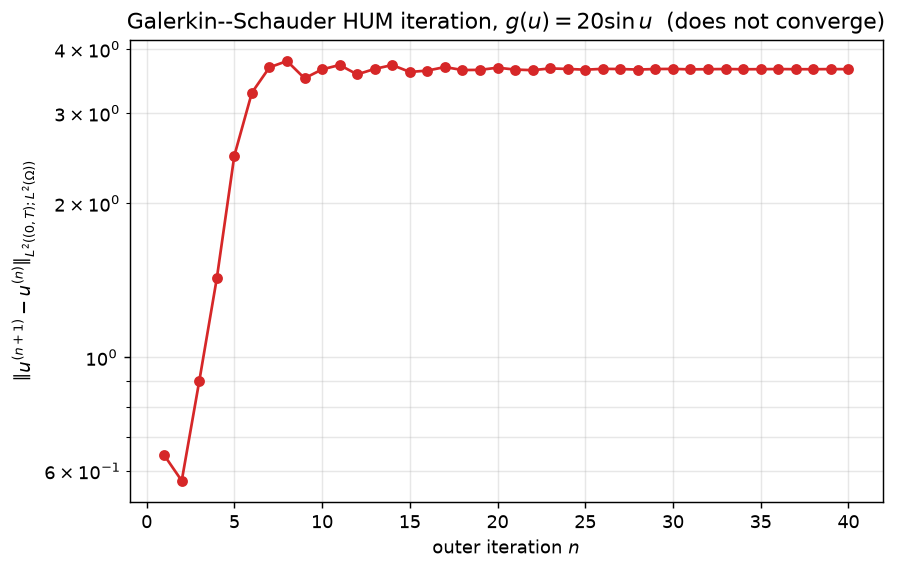
Neural-Spectral controller↩︎
The Neural-Spectral method of Section 2.1 applies without modification. We use the ansatz \[\widetilde{u}_{\theta_a}(t,x) = \sum_{j=1}^{P}a_j(t;\theta_a)e_j(x), \qquad \widetilde{f}_{\theta_c}(t,x)\,\mathbf{1}_\omega = \sum_{j=1}^{P}c_j(t;\theta_c)e_j(x)\,\mathbf{1}_\omega,\] with shallow per-mode networks of widths \[m_a=m_c=64.\] The residual 11 becomes \[R_j(t;\theta) = a_j''(t;\theta_a) + \omega_j^2a_j(t;\theta_a) + Q_j(t;\theta_a) +\sum_{\ell=1}^P M_{j\ell}\,c_\ell(t;\theta_c), \qquad j=1,\ldots,P,\] where \[Q_j(t;\theta_a) := \int_\Omega g\left( \sum_{\ell=1}^{P}a_\ell(t;\theta_a)e_\ell(x) \right)e_j(x)\,dx .\] The nonlinear Galerkin terms \(Q_j\) are evaluated by composite trapezoidal quadrature on \(257\) spatial nodes. Training uses \(250\) collocation points, endpoint weights \[\lambda_{\mathrm{IC}}=\lambda_{\mathrm{TC}}=500,\] \(3000\) Adam steps, followed by \(12\) blocks of \(400\) L-BFGS iterations. The total wall time is approximately \(90\) seconds on a single CPU.
Result at \(\beta=20\)↩︎
A crucial point of interpretation is that exact controllability is fundamentally a feasibility statement. Even in a finite-dimensional Galerkin space, there may be many valid state-control pairs satisfying both the projected dynamics and the required endpoint conditions. Indeed, note that the overlap matrix \(M_P = \left(M_{j\ell}\right)_{j,\ell=1}^P\) is positive definite. For any nonzero vector \(\xi\in\mathbb{R}^P\), we have \[\xi^T M_P \xi = \int_{\omega_\delta} \left|\sum_{j=1}^P \xi_j e_j(x,y)\right|^2 \,dx\,dy > 0.\] The strict inequality holds because a nontrivial finite linear combination of Dirichlet eigenfunctions cannot vanish identically on the open set \(\omega_\delta\). Consequently, \(M_P\) is invertible. Thus, given a sufficiently smooth modal path \[\widetilde{u}(t,x) = \sum_{j=1}^{P}a_j(t)e_j(x)\] satisfying the prescribed initial and terminal conditions, the equation \[\sum_{\ell=1}^P M_{j\ell}\,c_\ell(t;\theta_c) = -\left(a_j''(t)+\omega_j^2a_j(t)+Q_j(t)\right), \qquad j=1,\ldots,P,\] uniquely defines a control vector that forces the projected residual to vanish. Different choices of the path \(\left\{a_j(t)\right\}_{j=1}^P\) therefore generate different admissible controls. The loss 12 does not contain a minimum-energy selection principle; it seeks a dynamically consistent control-state pair satisfying the endpoint constraints. Thus, the learned control should be judged by whether it actually steers the nonlinear dynamics to the target, rather than by its proximity to the nonconverged HUM-S iterate.
In the reported run, the Neural-Spectral optimization converges to a small residual and yields a forward-validated steering control. The final diagnostics are reported in Table 1. The self-reported terminal error from the network is exceptionally small \(\left(3.13 \times 10^{-3}\right)\). More importantly, the forward-validation error, obtained by independently integrating the full nonlinear semi-discrete system using the recovered control with a high-accuracy DOP853 solver, is \(4.33 \times 10^{-1}\). Combined with a low accumulated residual sum \(\left(5.89 \times 10^{-1}\right)\), this demonstrates that the recovered control genuinely steers the physical system. This forward-validation error is nearly one order of magnitude smaller than the terminal error \(2.90\) obtained from the nonconverged HUM-S iterate.
| Quantity | Value |
|---|---|
| \(\left\|\widetilde{\Phi}(T,\cdot)-\Phi_T\right\|_{\mathcal{E}}\) (network output) | \(3.13 \times 10^{-3}\) |
| \(\left\|\Phi(T,\cdot)-\Phi_T\right\|_{\mathcal{E}}\) (forward validation) | \(4.33 \times 10^{-1}\) |
| \(\displaystyle \sum_{j=1}^{P}\|R_j(\cdot;\theta)\|_{L^2(0,T)}^2\) | \(5.89\times10^{-1}\) |
The learned control is shown in Figure 2. Panel (a) displays the spectral coefficients \(c_j(t)\), \(j=1,\ldots,P\). Panel (b) shows the corresponding spatial profile \[\widetilde{f}_{\theta_c}(t,x) = \sum_{j=1}^{P}c_j(t)e_j(x)\] at three intermediate times. The shaded band marks the actuator region \(\omega_{\delta}=(0,0.3) \cup (0.3,0.7)\).
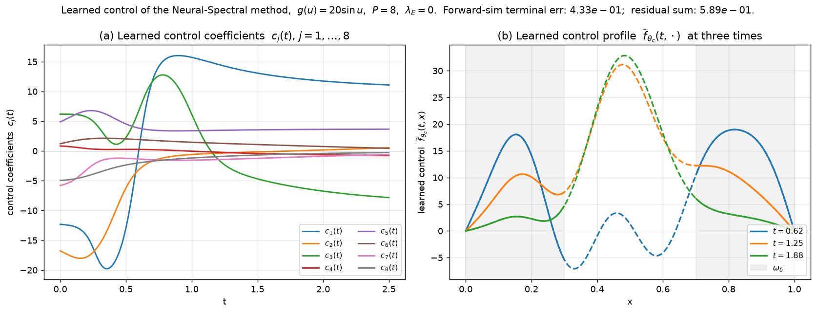
Remark 18 (Interpretation of the comparison). The failure observed above is not a failure of HUM theory itself. It is the failure of a particular Galerkin–Schauder fixed-point implementation in a strongly nonlinear regime. This distinction is important. For small Lipschitz constants, the frozen-source HUM map behaves contractively, and the iteration converges. For \(\beta=20\), the effective contraction property is lost, and the iterates fail to stabilize. Our Neural-Spectral method uses a different mechanism. It does not iterate a linearized HUM map. Instead, it directly minimizes the residual and endpoint mismatch over a joint state-control parameterization. The Lipschitz constant \(L_g\) affects the conditioning and nonconvexity of this optimization problem, but it does not enter through a global contraction requirement. This explains why the Neural-Spectral formulation can still find a useful steering control in a regime where the tested HUM-S implementation does not converge, in agreement with the approximation results of Theorems 5 and 8.
4.2 2D wave equation: Neural-Spectral method vs.standard PINN↩︎
In the previous sections, the Neural-Spectral method was compared against the classical Galerkin–Schauder HUM iteration, which is the natural reference within the spectral framework. Here we step outside the spectral framework and compare against a different, widely used family of PDE-constrained learning methods: physics-informed neural networks (PINNs) in the joint \((t,x,y)\) variables. The question is operational: at comparable parameter count and wall time, how does a standard soft-constrained PINN perform on the controlled wave equation in a genuinely two-dimensional spatial domain?
Problem↩︎
We consider 1 on \[\Omega=(0,1)^2\] with the boundary-collar actuator domain \[\omega_\delta = \left\{ (x,y)\in\Omega: \min\{x,1-x,y,1-y\}<\delta \right\}, \qquad \delta=0.3.\] Equivalently, \[\omega_\delta = \Omega\setminus[\delta,1-\delta]^2 = \Omega\setminus[0.3,0.7]^2.\] Thus, \(\omega_\delta\) is the shell of width \(0.3\) adjacent to \(\partial\Omega\), and \[|\omega_\delta| = 1-(1-2\delta)^2 = 1-0.4^2 = 0.84.\] Hence, the actuator domain occupies \(84\%\) of \(\Omega\). We take \[T=7,\qquad \alpha=0,\] and no nonlinearity, \[g\equiv0.\] The controlled equation is therefore \[u_{tt}-\Delta u+f\,\mathbf{1}_{\omega_\delta}=0 \quad\text{on }(0,T)\times\Omega, \qquad u|_{\partial\Omega}=0.\]
The actuator \(\omega_\delta\) is compatible with the Geometric Control Condition (GCC). Indeed, a unit-speed ray that has not entered \(\omega_\delta\) must remain inside the central square \([\delta,1-\delta]^2\). Let \(v = (v_1, v_2)\) be the direction vector of this unit-speed ray, which implies its Euclidean norm is \(\|v\|_{\mathbb{R}^2} = \sqrt{v_1^2 + v_2^2} = 1\). Since \(v_1^2 + v_2^2 \le 2\max\left\{|v_1|^2, |v_2|^2\right\}\), it immediately follows that \[\max\{|v_1|,|v_2|\}\ge \frac{1}{\sqrt2}.\] Moreover, the maximum distance the ray can travel along any coordinate axis while remaining inside the central square is exactly its side length, \(1-2\delta\). Therefore, the total time \(T_\delta\) the ray can spend inside the central square is bounded by the time it takes to exit along the fastest coordinate direction, that is, \[T_\delta \le \min\left\{ \frac{1-2\delta}{|v_1|}, \frac{1-2\delta}{|v_2|} \right\} = \frac{1-2\delta}{\max\{|v_1|,|v_2|\}} \le \sqrt2(1-2\delta).\] For \(\delta=0.3\), this gives \[T_\delta\le0.4\sqrt2\approx0.566.\] Thus, the choice \(T=7\) is safely above this sufficient GCC time.
The initial data are \[u^0(x,y) = \sin(\pi x)\sin(\pi y) + \frac{1}{2}\sin(\pi x)\sin(2\pi y), \qquad u^1\equiv0,\] and the target state is \[\left(u_T^0,u_T^1\right) \equiv (0,0).\] The \(L^2(\Omega)\)-orthonormal Dirichlet sine basis is \[e_{j,k}(x,y) = 2\sin(j\pi x)\sin(k\pi y), \qquad j,k\in\mathbb{N}^*,\] with eigenvalues \[\mu_{j,k} = \left(j^2+k^2\right)\pi^2.\] We use the spectral truncation \[j,k\in\{1,2,3,4\},\] that is, \(P_{\max}^2=16\) retained modes for the spectral method. The PINN itself is not spectrally truncated during training.
Let \(m=(j,k)\) and \(n=(j',k')\) denote multi-indices in \(\{1,2,3,4\}^2\). If the lifted control field is written as \[\widetilde{f}(t,x,y) = \sum_n c_n(t)e_n(x,y),\] then the actual applied control is \[\mathbf{1}_{\omega_\delta}\widetilde{f}.\] The projected dynamics are \[\label{eq:test6-spec-ode} \ddot a_m(t)+\mu_m a_m(t)+\sum_n M_{mn}c_n(t)=0, \qquad m\in\{1,2,3,4\}^2,\tag{49}\] where \[M_{mn} = \int_{\omega_\delta} e_m(x,y)e_n(x,y)\,dx\,dy.\] For \(\delta=0.3\), the overlap matrix \(M\) has eigenvalues in \[[0.085,1.000]\] and condition number approximately \(11.7\), so the retained finite-dimensional control problem is well-conditioned.
The energy norm of the initial data is \[\left\|\left(u^0,u^1\right)\right\|_{\mathcal{E}}^2 = 2\pi^2\left(\frac{1}{2}\right)^2 + 5\pi^2\left(\frac{1}{4}\right)^2 \approx 8.02,\] and therefore \[\left\|\left(u^0,u^1\right)\right\|_{\mathcal{E}}\approx2.83.\] Since the target is zero and the uncontrolled linear wave equation conserves energy, any control that has a negligible effect on the dynamics will produce a forward-simulation terminal error close to this value.
Method 1: Neural-Spectral method↩︎
For each retained mode \((j,k)\in\{1,\ldots,4\}^2\), we use two independent shallow \(\tanh\) networks of width \(64\), \[a_{j,k}(t;\theta_a), \qquad c_{j,k}(t;\theta_c),\] for the state coefficient and the lifted-control coefficient. The parameters are trained by minimizing the unsupervised projected residual loss \[\begin{align} &\mathcal{L}_{\mathrm{spec}}(\theta_a,\theta_c) = \int_0^T \sum_m \left| \ddot a_m(t;\theta_a) + \mu_m a_m(t;\theta_a) + \sum_n M_{mn}c_n(t;\theta_c) \right|^2 \,dt \\ &+\lambda\left(\left\| \sum_{m} \left(a_m(0;\theta_a), \dot{a}_m(0;\theta_a)\right)e_j-\left(u^0, u^1\right) \right\|_{\mathcal{E}}^2 + \left\| \sum_{m}\left(a_m(T;\theta_a),\dot{a}_m(T;\theta_a)\right)e_j-\left(u_T^0, u_T^1\right) \right\|_{\mathcal{E}}^2\right), \end{align}\] with \(\lambda=100\). The initial and terminal mismatch terms are measured in the energy norm. The residual is the projected PDE residual of 49 ; consequently, driving this residual to zero together with the endpoint constraints yields a true solution of the retained truncated system.
In the present experiment, \[u^1\equiv0, \qquad (u_T^0,u_T^1)=(0,0),\] so this loss reduces to \[\begin{align} \mathcal{L}_{\mathrm{spec}}(\theta_a,\theta_c) =&{} \int_0^T \sum_m \left| \ddot a_m(t;\theta_a) + \mu_m a_m(t;\theta_a) + \sum_n M_{mn}c_n(t;\theta_c) \right|^2 \,dt \\ &+\lambda\left(\left\| \sum_{m} \left(a_m(0;\theta_a), \dot{a}_m(0;\theta_a)\right)e_j-\left(u^0, 0\right) \right\|_{\mathcal{E}}^2 + \left\| \sum_{m}\left(a_m(T;\theta_a),\dot{a}_m(T;\theta_a)\right)e_j \right\|_{\mathcal{E}}^2\right). \end{align}\]
The training schedule uses \(250\) time-collocation points, \(2000\) Adam steps, followed by \(25\) blocks of \(300\) L-BFGS iterations. The total number of trainable parameters is \(6144\).
Remark 19. The choice of penalty weight \(\lambda=100\) is motivated by the need to mitigate gradient pathologies during the optimization process. Empirically, the gradients with respect to the PDE residual often exhibit significantly larger magnitudes than those associated with the initial and terminal conditions. By assigning heavier weights to the latter, we ensure that the network prioritizes the given initial and terminal constraints. This prevents the optimizer from converging to trivial, physically meaningless solutions that satisfy the interior PDE dynamics but violate the prescribed data.
Method 2: PINN in \((t,x,y)\)↩︎
The PINN baseline uses two fully connected feedforward networks with \(\tanh\) activations, width \(40\), and depth \(4\): \[u_\theta:\mathbb{R}^3\to\mathbb{R}, \qquad f_\theta:\mathbb{R}^3\to\mathbb{R}.\] The first network represents the state, and the second represents the control field. The actuator is imposed through the indicator \[\chi_{\omega_\delta}(x,y) = \mathbf{1}_{\{\min\{x,\,1-x,\,y,\,1-y\}<\delta\}}.\]
Let \[\mathcal{G}_{\mathrm{int}} = \{(t_q,x_q,y_q)\}_{q=1}^{N_{\mathrm{int}}} \subset (0,T)\times\Omega\] be the interior collocation set for the PDE residual, \[\mathcal{G}_{\mathrm{bc}} = \{(t_q,x_q,y_q)\}_{q=1}^{N_{\mathrm{bc}}} \subset (0,T)\times\partial\Omega\] be the boundary collocation set for the homogeneous Dirichlet condition, and \[\mathcal{G}_{\mathrm{ep}} = \{(x_q,y_q)\}_{q=1}^{N_{\mathrm{ep}}} \subset \Omega\] be the endpoint grid used at \(t=0\) and \(t=T\). To solve this control problem using the standard PINN framework (as originally introduced by Raissi et al. [13]), we reformulate the constrained PDE system into an unconstrained multi-objective optimization problem. The physical laws and boundary constraints are enforced as soft penalty terms in the empirical loss function. The explicit PINN loss is \[\begin{align} \mathcal{L}_{\mathrm{PINN}}(\theta) ={}& \Lambda_{\mathrm{PDE}} \frac{1}{N_{\mathrm{int}}} \sum_{q=1}^{N_{\mathrm{int}}} \left| \partial_{tt}u_\theta(t_q,x_q,y_q) - \partial_{xx}u_\theta(t_q,x_q,y_q) - \partial_{yy}u_\theta(t_q,x_q,y_q) + f_\theta(t_q,x_q,y_q)\chi_{\omega_\delta}(x_q,y_q) \right|^2 \\ &+ \Lambda_{\mathrm{BC}} \frac{1}{N_{\mathrm{bc}}} \sum_{q=1}^{N_{\mathrm{bc}}} \left| u_\theta(t_q,x_q,y_q) \right|^2 \\ &+ \Lambda_{\mathrm{IC}} \frac{1}{N_{\mathrm{ep}}} \sum_{q=1}^{N_{\mathrm{ep}}} \left[ \left| u_\theta(0,x_q,y_q)-u^0(x_q,y_q) \right|^2 + \left| \partial_t u_\theta(0,x_q,y_q)-u^1(x_q,y_q) \right|^2 \right] \\ &+ \Lambda_{\mathrm{TC}} \frac{1}{N_{\mathrm{ep}}} \sum_{q=1}^{N_{\mathrm{ep}}} \left[ \left| u_\theta(T,x_q,y_q)-u_T^0(x_q,y_q) \right|^2 + \left| \partial_t u_\theta(T,x_q,y_q)-u_T^1(x_q,y_q) \right|^2 \right]. \end{align}\] In the present experiment, \[u^1\equiv0, \qquad (u_T^0,u_T^1)=(0,0),\] so this loss reduces to \[\begin{align} \mathcal{L}_{\mathrm{PINN}}(\theta) ={}& \Lambda_{\mathrm{PDE}} \frac{1}{N_{\mathrm{int}}} \sum_{q=1}^{N_{\mathrm{int}}} \left| \partial_{tt}u_\theta(t_q,x_q,y_q) - \partial_{xx}u_\theta(t_q,x_q,y_q) - \partial_{yy}u_\theta(t_q,x_q,y_q) + f_\theta(t_q,x_q,y_q)\chi_{\omega_\delta}(x_q,y_q) \right|^2 \\ &+ \Lambda_{\mathrm{BC}} \frac{1}{N_{\mathrm{bc}}} \sum_{q=1}^{N_{\mathrm{bc}}} \left| u_\theta(t_q,x_q,y_q) \right|^2 \\ &+ \Lambda_{\mathrm{IC}} \frac{1}{N_{\mathrm{ep}}} \sum_{q=1}^{N_{\mathrm{ep}}} \left[ \left| u_\theta(0,x_q,y_q)-u^0(x_q,y_q) \right|^2 + \left| \partial_t u_\theta(0,x_q,y_q) \right|^2 \right] \\ &+ \Lambda_{\mathrm{TC}} \frac{1}{N_{\mathrm{ep}}} \sum_{q=1}^{N_{\mathrm{ep}}} \left[ \left| u_\theta(T,x_q,y_q) \right|^2 + \left| \partial_t u_\theta(T,x_q,y_q) \right|^2 \right]. \end{align}\] We use \[\Lambda_{\mathrm{PDE}}=50, \qquad \Lambda_{\mathrm{BC}} = \Lambda_{\mathrm{IC}} = \Lambda_{\mathrm{TC}} = 100.\] The total number of trainable parameters is \(6962\).
Remark 20. Consistent with the weighting strategy employed in the Neural-Spectral method above, we assign heavier penalties to the data constraints (\(\Lambda_{\mathrm{BC}} = \Lambda_{\mathrm{IC}} = \Lambda_{\mathrm{TC}} = 100\)) compared to the interior residual (\(\Lambda_{\mathrm{PDE}} = 50\)). This ensures the model strictly respects the boundary, initial, and terminal data, steering the optimization process away from physically meaningless, trivial solutions.
After training, the recovered PINN control \(f_\theta(t,x,y)\) is evaluated by forward validation. For this purpose, we project the applied control \(f_\theta\mathbf{1}_{\omega_\delta}\) onto the retained sine basis: \[d_{j,k}(t) = \int_{\omega_\delta} f_\theta(t,x,y)e_{j,k}(x,y)\,dx\,dy, \qquad j,k\in\{1,2,3,4\}.\] The validation dynamics are then \[\ddot a_{j,k}(t)+\mu_{j,k}a_{j,k}(t)+d_{j,k}(t)=0, \qquad j,k\in\{1,2,3,4\}.\] Thus, both methods are evaluated by inserting their recovered controls into the corresponding projected wave dynamics and measuring the terminal energy error.
Results↩︎
The single-problem comparison is summarized in Table 2, and the error-versus-wall-time trajectories are shown in Figure 3.
| method | forward-simulation error in \(\mathcal{E}\) | \(\left\|\mathbf{1}_{\omega_\delta}\widetilde{f}\right\|_{L^2((0,T)\times\Omega)}\) | \(n_{\mathrm{params}}\) | wall-time |
|---|---|---|---|---|
| Neural-Spectral (Method 1) | \(\mathbf{{4.84\times10^{-1}}}\) | \(11.92\) | \(6144\) | \(107\) s |
| PINN \((t,x,y)\) (Method 2) | \(2.78\times10^{0}\) | \(0.21\) | \(6962\) | \(71\) s |
![Figure 3: Two-dimensional wave-equation comparison on the GCC-compatible boundary collar \omega_\delta=\Omega\setminus[0.3,0.7]^2, with T=7. (a): Final forward-simulation terminal error in \mathcal{E} for the two methods, shown on a logarithmic scale. The dotted line is the free-evolution baseline \|u^0\|_{\mathcal{E}}\approx2.83. The Neural-Spectral method reaches 4.84\times10^{-1}, while the PINN remains close to the baseline. (b): Time-resolved checkpoints of the forward-simulation error during training. The Neural-Spectral error decreases steadily over the training run, whereas the PINN error remains close to the free-evolution baseline.](/article/2606.28029/test6_plot.png "fig:")
What we found↩︎
(F1) The Neural-Spectral method is more accurate on this test. It reduces the forward-simulation terminal error from the free-evolution baseline \[\left\|u^0\right\|_{\mathcal{E}}\approx2.83\] to \[4.84\times10^{-1}.\] The PINN ends at \[2.78,\] which is only a modest reduction from the free-evolution baseline. Thus, on this benchmark, the Neural-Spectral method improves the terminal error by a factor of approximately \(5.7\) relative to the PINN.
(F2) The standard PINN baseline returns a weak control in this test. The recovered PINN control has applied \(L^2\)-norm \(0.21\), about \(57\) times smaller than that recovered by the Neural-Spectral method. The resulting learned pair behaves close to a free-evolution solution: it satisfies the wave equation, boundary condition, and initial condition reasonably well, but the recovered control is not strong enough to steer the state close to the terminal target.
(F3) The Neural-Spectral loss is aligned with the validated dynamics. The Neural-Spectral method optimizes the projected residual of 49 , which is the same finite-dimensional dynamics used in the forward-validation step. Thus, for the retained modal system, a small projected residual together with a small endpoint mismatch is directly relevant to the reported forward-validation error. By contrast, the PINN baseline uses a soft multi-objective loss in the physical variables, where the PDE residual, boundary condition, initial condition, and terminal condition enter as competing penalty terms. The observed weak-control solution is consistent with known optimization difficulties for PINNs, including gradient imbalance among loss components [21]. We do not claim that all PINN variants would behave similarly; rather, this experiment shows that the standard soft-constrained PINN used here is less effective than the Neural-Spectral formulation on this benchmark.
Remark 21. Both methods are tested on the same controlled wave equation using a comparable number of trainable parameters. The Neural-Spectral method benefits from building the Dirichlet eigenbasis and the modal control structure into the approximation from the beginning. This reduces the optimization problem to the learning of time-dependent trajectories for finitely many modal coefficients. The PINN baseline, by contrast, learns the full space-time state and control fields directly from soft penalties. In this oscillatory benchmark, the difference in parameterization and loss alignment appears to be a significant factor in the observed accuracy gap.
4.3 3D wave equation: Neural-Spectral method vs. DeepONet↩︎
The previous sections compared the Neural-Spectral method against either the classical Galerkin–Schauder HUM iteration in one-dimensional spatial domain or, in the two-dimensional case, a standard PINN. We now compare it against a different family of neural PDE solvers: operator-learning methods, with DeepONet [38] as a representative example. The test is performed on the linear three-dimensional wave equation. The purpose is operational: we compare a per-problem solver, namely the Neural-Spectral method, with an operator-learning surrogate that is trained once and then reused. Thus, the two methods occupy different positions in the cost-accuracy trade-off. We first compare them on a single three-dimensional control problem, and then examine what changes when the same trained DeepONet is reused on a second related problem.
Problem↩︎
We consider 1 on the three-dimensional unit cube \[\Omega=(0,1)^3,\] with no nonlinearity, \(g\equiv0\), and with \(\alpha=0\). The initial velocity is zero, \(u^1\equiv0\), and the target state is \[\left(u_T^0,u_T^1\right)=(0,0).\] The control acts on the boundary collar \[\omega_\delta = \left\{ (x,y,z)\in\Omega: \min\{x,1-x,y,1-y,z,1-z\}<\delta \right\}, \qquad \delta=0.3,\] and we take \(T=5\). Equivalently, \[\omega_\delta = \Omega\setminus[\delta,1-\delta]^3.\] For \(\delta=0.3\), this gives \[|\omega_\delta| = 1-(1-2\delta)^3 = 1-0.4^3 = 0.936,\] so the controlled domain occupies approximately \(93.6\%\) of the cube.
This choice is compatible with the Geometric Control Condition (GCC). Indeed, a unit-speed ray that has not yet entered \(\omega_\delta\) must remain inside the central cube \([\delta,1-\delta]^3\). If \(v=(v_1,v_2,v_3)\) is its direction, then \(\|v\|_{\mathbb{R}^3}=1\). As \(v_1^2+v_2^2+v_3^2 \le 3\max\limits_{1\le i\le3}|v_i|^2\), it holds that \[\max\limits_{1\le i\le3}|v_i|\ge \dfrac1{\sqrt3}.\] Moreover, the maximum distance the ray can travel along any coordinate axis while remaining inside the central square is exactly its side length, \(1-2\delta\). Therefore, the total time \(T_\delta\) the ray can spend inside the central square is strictly bounded by the time it takes to exit along the fastest coordinate direction, that is, \[T_\delta \le \min\limits_{1\le i\le3}\frac{1-2\delta}{|v_i|} = \frac{1-2\delta}{\max\limits_{1\le i\le3}|v_i|} \le \sqrt3(1-2\delta).\] For \(\delta=0.3\), this gives \[T_\delta\le 0.4\sqrt3\approx0.693.\] Thus, the choice \(T=5\) is safely above this sufficient GCC time.
The \(L^2(\Omega)\)-orthonormal Dirichlet sine basis is \[e_{j,k,\ell}(x,y,z) = \left(\sqrt2\right)^3 \sin(j\pi x)\sin(k\pi y)\sin(\ell\pi z), \qquad j,k,\ell\in\mathbb{N}^*,\] with eigenvalues \[\mu_{j,k,\ell} = \left(j^2+k^2+\ell^2\right)\pi^2.\] We use the spectral truncation \[1\le j,k,\ell\le P_{\max}=3,\] which gives \[n_{\mathrm{mode}}=P_{\max}^3=27\] retained modes.
Let \(m=(j,k,\ell)\) and \(n=(j',k',\ell')\) denote multi-indices in \(\{1,2,3\}^3\). If the lifted control field is written as \[\widetilde{f}(t,x,y,z) = \sum_n c_n(t)e_n(x,y,z),\] then the actual applied control is \[\mathbf{1}_{\omega_\delta}\widetilde{f}.\] The projected dynamics are \[\label{eq:test8-spec-ode} \ddot a_m(t)+\mu_m a_m(t)+\sum_n M_{mn}c_n(t)=0, \qquad m\in\{1,2,3\}^3,\tag{50}\] where \[M_{mn} = \int_{\omega_\delta} e_m(x,y,z)e_n(x,y,z)\,dx\,dy\,dz.\] For this actuator, the overlap matrix \(M\) has eigenvalues in \[[0.125,0.999]\] and condition number approximately \(8.0\), so the retained finite-dimensional control problem is well-conditioned. We use two test problems, each with nonzero spectral content in four low modes: \[\text{Test \#1:}\quad \left\|u^0\right\|_{\mathcal{E}}=1.15, \qquad \text{Test \#2:}\quad \left\|u^0\right\|_{\mathcal{E}}=1.06.\]
Method 1: Neural-Spectral method↩︎
For each retained spectral mode \(m\), we represent both the state coefficient \(a_m(t)\) and the lifted-control coefficient \(c_m(t)\) by shallow \(\tanh\) networks of width \(64\). The parameters \(\theta_a\) and \(\theta_c\) are trained by minimizing the projected residual loss \[\begin{align} \mathcal{L}_{\mathrm{spec}}(\theta_a,\theta_c) ={}& \int_0^T \sum_{j=1}^{3}\sum_{k=1}^{3}\sum_{\ell=1}^{3} \left| \ddot a_{j,k,\ell}(t;\theta_a) + \left(j^2+k^2+\ell^2\right)\pi^2 a_{j,k,\ell}(t;\theta_a) \right.\\ &\left. + \sum_{j'=1}^{3}\sum_{k'=1}^{3}\sum_{\ell'=1}^{3} M_{(j,k,\ell),(j',k',\ell')} c_{j',k',\ell'}(t;\theta_c) \right|^2 \,dt \\ &+ \Lambda \sum_{j=1}^{3}\sum_{k=1}^{3}\sum_{\ell=1}^{3} \left[ \left(j^2+k^2+\ell^2\right)\pi^2 \left|a_{j,k,\ell}(0;\theta_a)-u^0_{j,k,\ell}\right|^2 + \left|\dot{a}_{j,k,\ell}(0;\theta_a)\right|^2 \right] \\ &+ \Lambda \sum_{j=1}^{3}\sum_{k=1}^{3}\sum_{\ell=1}^{3} \left[ \left(j^2+k^2+\ell^2\right)\pi^2 \left|a_{j,k,\ell}(T;\theta_a)\right|^2 + \left|\dot{a}_{j,k,\ell}(T;\theta_a)\right|^2 \right], \end{align}\] where the initial and terminal mismatch terms are measured in the energy norm and \(\Lambda=100\). We use \(250\) time-collocation points, \(2000\) Adam steps, followed by \(18\) blocks of \(250\) L-BFGS iterations. The total number of trainable parameters is \(10\,368\). This method is trained from scratch for each test problem.
Method 2: DeepONet forward surrogate and gradient-descent control↩︎
The DeepONet is trained to approximate the finite-dimensional control-to-terminal-state map \[\mathcal{G}: c \longmapsto \left(u(T,\cdot),u_t(T,\cdot)\right),\] where \(c\) denotes the vector of piecewise-linear modal control coefficients and the initial data are zero. Since the wave equation is linear in this experiment, the terminal state for arbitrary initial data decomposes as \[(u(T,\cdot),u_t(T,\cdot)) = \left(u_{\mathrm{free}}(T,\cdot),v_{\mathrm{free}}(T,\cdot)\right) + \mathcal{G}(c).\] Thus, the same trained DeepONet can be reused for different initial and target states on the same domain. No HUM solver is used to generate the training labels; all labels are obtained from forward simulations of random controls.
4.3.0.1 Control parameterization.
The modal control is parameterized as a piecewise-linear interpolant on \[N_{t,\mathrm{sub}}=11\] time knots, with one curve per retained spectral mode. Thus, the branch input is \[b = \left(c_{j,k,\ell}(t_n)\right)_{ 1\le j,k,\ell\le3,\;0\le n\le10} \in\mathbb{R}^{297}.\]
4.3.0.2 Network architecture.
We use a two-channel DeepONet of the form \[\mathcal{G}_\theta(c)(x,y,z) = \left( \beta_\theta(c)\cdot \tau_\theta^u(x,y,z), \, \beta_\theta(c)\cdot \tau_\theta^v(x,y,z) \right).\] The branch network \[\beta_\theta:\mathbb{R}^{297}\to\mathbb{R}^q\] is a four-layer \(\tanh\) MLP of width \(128\), with \(q=160\). The trunk network \[\tau_\theta:\mathbb{R}^3\to\mathbb{R}^{2q}\] is a five-layer \(\tanh\) MLP of width \(128\). The total number of trainable parameters is \(183\,138\), about \(18\) times that of the Neural-Spectral method.
4.3.0.3 Offline training phase.
We generate \(1500\) random control samples by drawing \[c_{j,k,\ell}(t_n)\sim\mathcal{N}\left(0,0.8^2\right)\] independently for each retained mode and time knot. Each sampled control is forward-simulated from zero initial data under 50 to obtain \[\left(a_m(T),\dot{a}_m(T)\right).\] The terminal fields \[u(T,\cdot), \qquad u_t(T,\cdot)\] are then reconstructed by spectral expansion at \(100\) random query points in \(\Omega\). Since the forcing is piecewise linear in time, the forced linear oscillator response can be computed in closed form; no ODE solver is needed for this data-generation step. Generating all \(1500\) training samples takes approximately \(0.4\) seconds.
The DeepONet is trained by minimizing the mean-squared error of the two terminal channels at the query points. The training schedule consists of \(10\,000\) Adam steps with batch size \(128\), initial learning rate \(2\cdot10^{-3}\), and decay factor \(0.5\) every \(1500\) steps. The offline training time is approximately \(17\) seconds.
4.3.0.4 Online inversion phase.
Given a test problem \[\left(u^0,u^1,u_T^0,u_T^1\right),\] the free-evolution terminal state is computed in closed form and evaluated on a fixed \(9^3=729\)-point grid in \(\Omega\). The control parameter vector \[c\in\mathbb{R}^{297}\] is initialized at zero and optimized by \(1500\) Adam steps with initial learning rate \(0.05\), with learning-rate decay. The loss is the mean-squared mismatch between \(\mathcal{G}_\theta(c)\) and the required terminal offset on the evaluation grid. During this phase, the DeepONet weights are frozen, and gradients are taken only with respect to the control vector \(c\). The online inversion time per test problem is approximately \(6\)–\(8\) seconds.
4.3.0.5 Forward validation.
For both methods, the recovered control is inserted into the true truncated modal system 50 , starting from the actual initial data. The system is then integrated with DOP853 to a relative tolerance \(10^{-12}\). We report the model-independent terminal error \[\left\|\Phi(T,\cdot)-\Phi_T\right\|_{\mathcal{E}} = \left( \sum_m \mu_m \left(a_m(T)-u^0_{T,m}\right)^2 + \left(\dot{a}_m(T)-u^1_{T,m}\right)^2 \right)^{1/2}.\] This is the same forward-validation metric used in the previous numerical tests.
Main result: single-problem accuracy↩︎
The main comparison is summarized in Table 3 and in Figure 4.
| method | forward-simulation error in \(\mathcal{E}\) | \(\left\|\mathbf{1}_{\omega_\delta}\widetilde{f}\right\|_{L^2((0,T)\times\Omega)}\) | wall-time |
|---|---|---|---|
| Neural-Spectral (Method 1) | \(\mathbf{4.39\times10^{-1}}\) | \(7.67\) | \(81\) s |
| DeepONet (Method 2) | \(1.36\times10^{0}\) | \(8.44\) | \(23\) s |
On Test #1, the Neural-Spectral method gives a terminal energy-norm error \[4.39\times10^{-1},\] whereas DeepONet gives \[1.36\times10^{0}.\] Thus, on this single problem, the Neural-Spectral method gives the smaller forward-validation terminal error, whereas DeepONet is faster in online wall time because part of the computation has been shifted into an offline-trained forward surrogate.
One possible source of the DeepONet error in this test is surrogate accuracy in the region of control space reached by the online inversion. During the online phase, the surrogate mismatch \[\|\mathcal{G}_\theta(c)-\text{target offset}\|^2\] on the evaluation grid is reduced to approximately \(10^{-2}\). However, when the resulting control is inserted into the true projected wave dynamics 50 , the forward-validation terminal error is \(1.36\times10^{0}\). This indicates that the optimized control is effective for the learned surrogate but less effective for the true finite-dimensional dynamics in this experiment. Such behavior is a known concern when learned forward operators are used inside inverse or control loops: the inversion step may move toward regions of input space where the surrogate is less accurate than its average training error suggests.
The Neural-Spectral method avoids this particular surrogate-error mechanism because it optimizes the residual of the same projected dynamics used in the forward-validation step. Its remaining errors come from finite spectral truncation, neural parameterization, numerical quadrature, and nonconvex optimization.
Additional observation: amortization across multiple problems↩︎
The above comparison treats the two methods on the same footing: each is asked to solve a single control problem. The natural regime for operator-learning methods, however, is the many-query setting, where the same trained surrogate is reused across multiple problems on the same domain. We therefore ran a second test, Test #2, with different initial data satisfying \[\left\|u^0\right\|_{\mathcal{E}}=1.06.\] The initial data places mass on the cross modes \[(2,2,1),\qquad (1,2,2),\qquad (3,1,1),\] as well as on \((1,1,1)\).
| Test #1 | Test #2 | |||
| method | fwd-err | wall-time | fwd-err | wall-time |
| Neural-Spectral (Method 1) | \(\mathbf{4.39\times10^{-1}}\) | \(81\) s | \(\mathbf{2.59\times10^{-1}}\) | \(291\) s |
| DeepONet (Method 2) | \(1.36\times10^{0}\) | \(23\) s | \(1.22\times10^{0}\) | \(13\) s |
| cumulative wall time over both tests | Neural-Spectral: \(372\) s | DeepONet: \(36\) s | ||
![Figure 4: 3D wave-equation comparison: Neural-Spectral vs. DeepONet on the GCC-compatible boundary collar \omega_\delta=\Omega\setminus[0.3,0.7]^3, with T=5. (a): Forward-simulation terminal error in \mathcal{E} on the two test problems, shown on a logarithmic scale. On both problems, the Neural-Spectral method is more accurate: by a factor of about 3.1 on Test #1 and about 4.7 on Test #2. The dotted lines mark the corresponding free-evolution baselines \left\|u^0\right\|_{\mathcal{E}}. (b): Wall-time breakdown. The DeepONet’s one-time offline cost (data generation plus training, hatched) is incurred only on the first problem; subsequent problems incur only the online inversion cost. The Neural-Spectral method retrains from scratch for each problem.](/article/2606.28029/test8_plot.png "fig:")
With two test problems, the Neural-Spectral method gives the smaller forward-validation terminal error on each individual problem, while DeepONet has the smaller cumulative wall time because its offline training cost is amortized. In general, if \(W_{\mathrm{spec}}\) denotes the average wall time of a single Neural-Spectral solve, \(W_{\mathrm{off}}\) the one-time DeepONet offline training cost, and \(W_{\mathrm{inf}}\) the DeepONet online inference cost per new problem, then the two cumulative costs over \(N\) related problems are approximately \[N W_{\mathrm{spec}} \qquad\text{and}\qquad W_{\mathrm{off}}+N W_{\mathrm{inf}}.\] Thus, DeepONet becomes faster when \[N> \frac{W_{\mathrm{off}}}{W_{\mathrm{spec}}-W_{\mathrm{inf}}}.\] With the present timings, this threshold is below one problem, so DeepONet is already faster in wall time on the first test. The observed trade-off in these experiments is therefore between per-instance forward-validation accuracy and amortized online speed.
Remark 22. The DeepONet accuracy could likely be improved by spending more compute in the offline phase, for instance, through a larger training set, a richer architecture, or an iterative-refinement loop in which the surrogate is fine-tuned near the controls returned by the inversion step. These modifications would increase the offline cost and may change the quantitative comparison. The present experiments, therefore, should be viewed as a comparison between one representative DeepONet surrogate and the proposed per-instance Neural-Spectral solver, rather than as a definitive comparison between spectral control reconstruction and operator learning in general. In the reported tests, the Neural-Spectral method gives terminal errors of order \(10^{-1}\), while DeepONet provides faster online inversion after offline training.
4.4 A two-dimensional linear Gramian reference benchmark↩︎
In this section, we include a linear reference benchmark for which the finite-dimensional Galerkin control can be computed explicitly through a controllability Gramian. The purpose of this test is different from the previous PINN and DeepONet comparisons. Here, we compare the Neural-Spectral reconstruction with a classical Gramian/HUM reference control for the same projected linear dynamics. This provides a non-machine-learning benchmark against which the accuracy of the recovered control can be assessed.
We consider the linear wave equation \[\label{eq:linear952d95wave95test} \begin{cases} u_{tt}-\Delta u+f\,\mathbf{1}_{\omega_\delta}=0, & (t,x,y)\in (0,T)\times \Omega,\\ u=0, & (t,x,y)\in (0,T)\times \partial\Omega,\\ u(0,x,y)=u^0(x,y),\qquad u_t(0,x,y)=u^1(x,y), & (x,y)\in \Omega, \end{cases}\tag{51}\] where \[\Omega=(0,1)^2,\qquad g\equiv 0,\qquad \alpha=0.\] The target is the null state \[u(T,\cdot)=0,\qquad u_t(T,\cdot)=0.\] We choose the boundary-collar actuator \[\omega_\delta = \Omega\setminus [\delta,1-\delta]^2 = \{(x,y)\in \Omega:\min(x,1-x,y,1-y)<\delta\},\] with \[\delta=0.2,\qquad T=4.\] The uncontrolled region is the central square \[[\delta,1-\delta]^2=[0.2,0.8]^2.\] For this collar geometry, any geometric ray traveling at unit speed that has not yet entered the control region must remain inside the central uncontrolled square. Thus, the distance such a ray can cover before hitting the collar is bounded by the diameter of this square, namely \((1-2\delta)\sqrt{2}\). Thus, the time before the unit-speed ray reaches the collar is also bounded by \[(1-2\delta)\sqrt 2=0.6\sqrt 2\approx 0.849.\] Since \(T=4\), the pair \((\omega_\delta,T)\) satisfies the Geometric Control Condition (GCC) with a large safety margin. This elementary bound is used only to justify the benchmark geometry; no claim of sharpness is needed here.
For the initial condition, we take a finite superposition of Dirichlet modes: \[u^0(x,y) = E_{1,2}(x,y) + 0.7E_{3,1}(x,y) + 0.4E_{2,3}(x,y), \qquad u^1(x,y)=0,\] where \[E_{m,n}(x,y)=2\sin(m\pi x)\sin(n\pi y)\] is the \(L^2(\Omega)\)-normalized Dirichlet eigenfunction associated with the eigenvalue \[\mu_{m,n}=\pi^2\left(m^2+n^2\right).\] All three active modes are already included at the smallest truncation \(P=8\). Indeed, the largest active eigenvalue is \(\mu_{2,3}=13\pi^2\), and the first eight Dirichlet modes on the square contain all modes with \(m^2+n^2\le 13\). Hence, the initial data is represented exactly at each truncation level \(P\in\{8,16,32\}\) used below, and the projected initial energy norm \(\|Y_0\|_{\mathcal{E}_P}\approx 10.87\) is independent of \(P\).
Using the spectral re-indexing bijection \(q: \mathbb{N}^* \to \mathbb{N}^* \times \mathbb{N}^*\) established in the proof of Lemma 2 (see Appendix 5), we map the two-dimensional eigenvalues \(\mu_{m,n}\) in ascending order. Let \(e_j(x,y) := E_{q(j)}(x,y)\) denote the corresponding sorted sequence of the first \(P\) Dirichlet eigenfunctions. We then write the Galerkin approximation as \[u_P(t,x,y)=\sum_{j=1}^P a_j(t)e_j(x,y), \qquad f_P(t,x,y)=\sum_{j=1}^P c_j(t)e_j(x,y).\] Projecting 51 onto \(\operatorname{span}\{e_1,\ldots,e_P\}\) gives \[a_j''(t)+\mu_j a_j(t) + \sum_{\ell=1}^P M_{j\ell}c_\ell(t)=0, \qquad j=1,\ldots,P,\] where \[M_{j\ell} = \int_{\omega_\delta} e_j(x,y)e_\ell(x,y)\,dx\,dy.\] In vector form, with \[a(t)=(a_1(t),\ldots,a_P(t))^T,\qquad c(t)=(c_1(t),\ldots,c_P(t))^T,\] and \[\Lambda_P=\operatorname{diag}(\mu_1,\ldots,\mu_P), \qquad M_P=\left(M_{j\ell}\right)_{j,\ell=1}^P,\] the projected system is \[a''(t)+\Lambda_P a(t)+M_Pc(t)=0.\] Equivalently, setting \[Y(t)= \begin{pmatrix} a(t)\\ a'(t) \end{pmatrix},\] we obtain the first-order controlled system \[\label{eq:linear952d95first95order95system} Y'(t)=A_PY(t)+B_Pc(t),\tag{52}\] where \[A_P= \begin{pmatrix} 0&I_P\\ -\Lambda_P&0 \end{pmatrix}, \qquad B_P= \begin{pmatrix} 0\\ -M_P \end{pmatrix}.\] For this boundary-collar actuator, \(M_P\) is positive definite. Indeed, for any nonzero vector \(\xi\in\mathbb{R}^P\), \[\xi^TM_P\xi = \int_{\omega_\delta} \left|\sum_{j=1}^P \xi_j e_j(x,y)\right|^2\,dx\,dy>0,\] because a nontrivial finite linear combination of Dirichlet eigenfunctions cannot vanish identically on the open set \(\omega_\delta\). Therefore, \(M_P\) is invertible. Consequently, \[\operatorname{rank}\,[B_P,A_PB_P]=2P,\] and by the Kalman’s controllability rank condition (see, e.g., [39]), the finite-dimensional Galerkin system is controllable.
We compute \(M_P\) in closed form by exploiting orthonormality on the full square. Since \(\displaystyle\int_\Omega e_je_\ell = \delta_{j\ell}\) and \(\omega_\delta\) is the complement of the tensor-product square \([\delta,1-\delta]^2\), \[M_P = I_P - O_x\odot O_y, \qquad (O_x)_{j\ell} = \int_\delta^{1-\delta} 2\sin(m_j\pi x)\sin(m_\ell\pi x)\,dx,\] and similarly for \(O_y\) in the \(n\)-indices, with \(\odot\) denoting entry-wise multiplication. Numerically, the smallest eigenvalue of \(M_P\) decreases as \(P\) grows, reflecting the weaker interaction of some high modes with the collar. For \(P=8,16,32\), we find \[\lambda_{\min}(M_P) \approx 2.5\times 10^{-2},\quad 3.5\times 10^{-3},\quad 6.2\times 10^{-5},\] respectively. Thus, \(M_P\) remains positive definite over the truncation levels used in this benchmark, although the increasing ill-conditioning is visible.
The finite-dimensional Gramian reference control is computed with respect to the modal coefficient norm \[\int_0^T |c(t)|_{\mathbb{R}^P}^2\,dt.\] Let \[Y_0= \begin{pmatrix} a(0)\\ a'(0) \end{pmatrix}, \qquad Y_T=0,\] and define \[\label{eq:linear952d95gramian} W_T = \int_0^T e^{A_P(T-s)}B_PB_P^T e^{A_P^T(T-s)}\,ds.\tag{53}\] Since the pair \((A_P,B_P)\) is controllable, \(W_T\) is symmetric positive definite. The corresponding minimum-energy control steering \(Y_0\) to \(0\) is \[\label{eq:linear952d95hum95control} c_P^{\textrm{HUM}}(t) = B_P^T e^{A_P^T(T-t)}W_T^{-1} \left( -Y_{\textrm{free}}(T) \right), \qquad Y_{\textrm{free}}(T)=e^{A_PT}Y_0.\tag{54}\] Equivalently, \[Y(T) = e^{A_PT}Y_0 + \int_0^T e^{A_P(T-s)}B_Pc_P^{\textrm{HUM}}(s)\,ds = 0.\] In our implementation, \(W_T\) is assembled by Simpson quadrature applied to 53 , using matrix exponentials for the homogeneous flow. The computed reference control 54 steers the Galerkin system to the origin to within \[\left\|Y^{\textrm{HUM}}(T)\right\|_{\mathcal{E}_P}\sim 10^{-8},\] so it provides a numerically accurate reference for the projected system.
4.4.0.1 Neural-Spectral control.
We compare this reference with the Neural-Spectral control \(c_P^{\textrm{NS}}\). For the finite-dimensional linear system, the formula 54 implies that each component of \(c_P^{\textrm{HUM}}\) is a finite linear combination of temporal harmonics \[\cos(\sqrt{\mu_k}\,t), \qquad \sin(\sqrt{\mu_k}\,t), \qquad k=1,\ldots,P.\] This motivates the following frequency-informed temporal representation: \[\label{eq:linear952d95ns95ansatz} c_{\theta,j}(t) = \Theta_{j,0} + \sum_{k=1}^P \Bigl[ \Theta_{j,2k-1}\cos(\sqrt{\mu_k}\,t) + \Theta_{j,2k}\sin(\sqrt{\mu_k}\,t) \Bigr],\tag{55}\] with learnable weights \(\Theta\in\mathbb{R}^{P\times(2P+1)}\). This dictionary should be viewed as a frequency-informed specialization of the Neural-Spectral temporal representation for this linear benchmark: the modal spatial representation and the reduced control objective are the same, but the generic trainable temporal network is replaced by a fixed feature map matched to the known wave frequencies.
Unlike the fully unconstrained Neural-Spectral formulation in previous sections (where the PDE residual is penalized as a soft constraint), here we employ a hard-constrained approach. Given \(c_\theta\), the state \(Y_\theta\) is propagated from \(Y_0\) through 52 using the same matrix-exponential discretization used for the reference computation. Thus, the projected dynamics and the initial condition are enforced through the finite-dimensional propagation. The control is therefore obtained by solely minimizing the reduced objective \[\label{eq:linear952d95ns95loss} \mathcal{L}_{\textrm{NS}}(\theta) = \bigl\|Y_\theta(T)\bigr\|_{\mathcal{E}_P}^2 + \lambda_{\textrm{reg}}\,\|c_\theta\|_{L^2(0,T;\mathbb{R}^P)}^2 , \qquad \lambda_{\textrm{reg}}=3\times 10^{-4}.\tag{56}\] The first term penalizes the terminal mismatch, while the second term biases the optimization toward lower-energy controls. For small terminal error and small regularization parameter, this penalized formulation approximates the constrained minimum-energy Galerkin control problem solved explicitly by the Gramian formula. Optimization uses Adam followed by L-BFGS. After training, the recovered control is validated by solving 52 forward with \(c_P^{\textrm{NS}}\) using a high-order adaptive integrator.
We report the forward-validation terminal error \[\left\|Y^{\textrm{NS}}(T)\right\|_{\mathcal{E}_P} = \left( \sum_{j=1}^P \mu_j \left|a_j^{\textrm{NS}}(T)\right|^2 + \sum_{j=1}^P \left|\left(a_j^{\textrm{NS}}\right)'(T)\right|^2 \right)^{1/2},\] the distance to the finite-dimensional HUM reference control, \[\left\|c_P^{\textrm{NS}}-c_P^{\textrm{HUM}}\right\|_{L^2(0,T;\mathbb{R}^P)},\] and the relative control norm \[\dfrac{\left\|c_P^{\textrm{NS}}\right\|_{L^2(0,T;\mathbb{R}^P)}} {\left\|c_P^{\textrm{HUM}}\right\|_{L^2(0,T;\mathbb{R}^P)}}.\]
| \(P\) | \(\left\|Y^{\textrm{NS}}(T)\right\|_{\mathcal{E}_P}\) | \(\left\|c_P^{\textrm{NS}}-c_P^{\textrm{HUM}}\right\|_{L^2}\) | \(\left\|c_P^{\textrm{NS}}\right\|_{L^2}/\left\|c_P^{\textrm{HUM}}\right\|_{L^2}\) | wall-time |
|---|---|---|---|---|
| \(8\) | \(1.14\times 10^{-2}\) | \(0.014\) | \(1.0004\) | \(51\) s |
| \(16\) | \(1.17\times 10^{-2}\) | \(0.078\) | \(1.0008\) | \(65\) s |
| \(32\) | \(7.09\times 10^{-3}\) | \(0.077\) | \(1.0004\) | \(97\) s |
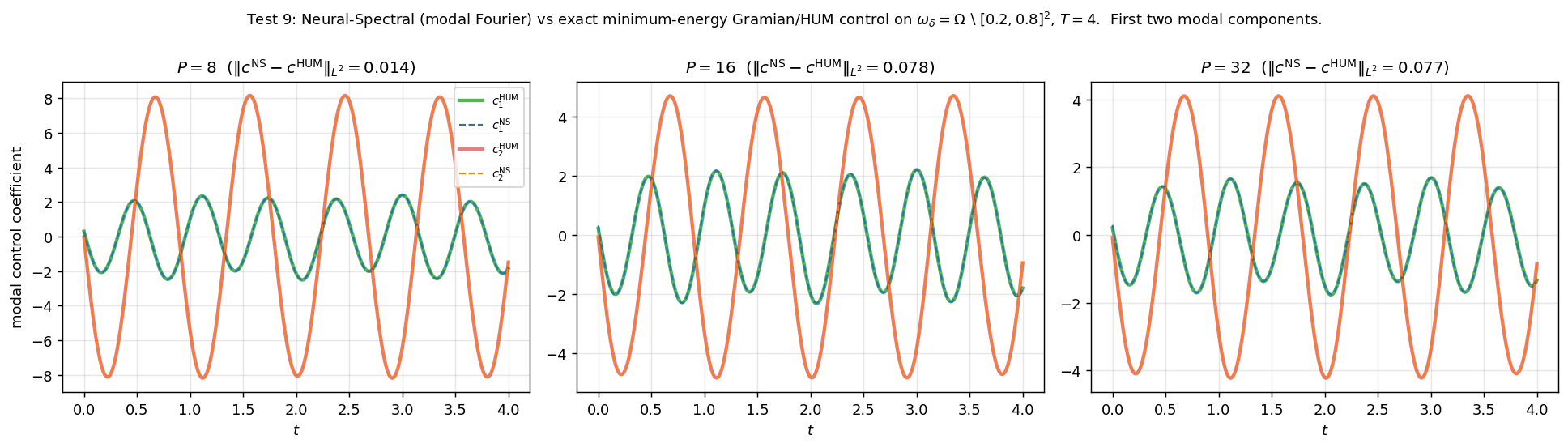
4.4.0.2 Discussion.
The results in Table 5 and Figure 5 show that the frequency-informed Neural-Spectral reconstruction is close to the classical finite-dimensional Gramian/HUM control in this linear reference benchmark. The relative control norm matches that of \(c_P^{\textrm{HUM}}\) to within roughly one part in a thousand across the reported truncation levels, and the modal control trajectories are visually close to the Gramian reference. The forward-validated terminal error is reduced by approximately three orders of magnitude relative to the free evolution \[\|Y_0\|_{\mathcal{E}_P}\approx 10.87,\] which is independent of \(P\) because the initial data is captured exactly at every truncation level.
Two structural points should be noted. First, this benchmark is favorable to the modal Fourier ansatz 55 . Since the finite-dimensional reference control is a linear combination of the temporal harmonics \[\left\{\cos\left(\sqrt{\mu_k}t\right),\sin\left(\sqrt{\mu_k}t\right):k=1,\ldots,P\right\},\] a feature map built from these frequencies has a small representation error for this linear problem. A generic time-network, by contrast, must learn the relevant oscillatory time scales during training. Second, the regularization in 56 plays an important selection role. The projected system is controllable, so many admissible controls may steer \(Y_0\) to the origin. The regularized objective biases the optimization toward lower-energy controls, and in this benchmark, the resulting control is close to the Gramian/HUM reference.
Unlike the PINN and DeepONet comparisons, this benchmark does not depend on another learned solver. The comparison is made against the finite-dimensional Gramian/HUM control of the same projected linear dynamics. The close agreement with \(c_P^{\textrm{HUM}}\), together with a small forward-validation terminal error, provides a useful consistency check for the Neural-Spectral control formulation in a setting where a classical reference solution is available.
4.4.0.3 Effect of the temporal ansatz.
The convergence study above uses the modal Fourier dictionary 55 for the temporal representation, whereas the general Neural-Spectral formulation in this paper represents each modal coefficient with a shallow, trainable time-network. To quantify the effect of using frequency-informed temporal features, we repeat the benchmark at fixed \(P=16\) with both ansatzes. Both variants are trained with the same reduced objective 56 , the same optimizer schedule, and the same finite-dimensional state propagation. For the tanh ansatz, each modal control coefficient is represented as \[c_{\theta,j}(t) = \sum_{r=1}^{m} A_{j,r}\tanh\bigl(W_{j,r}\,t+B_{j,r}\bigr), \qquad m=64,\] with all of \(A,W,B\) trained. The results are reported in Table 6 and Figure 6, where the relative control error is \[\dfrac{\left\|c_P^{\textrm{NS}}-c_P^{\textrm{HUM}}\right\|_{L^2}} {\left\|c_P^{\textrm{HUM}}\right\|_{L^2}}.\]
| method | terminal error | relative control error | wall-time |
|---|---|---|---|
| Neural-Spectral, tanh time networks | \(7.94\times 10^{-3}\) | \(1.185\) | \(132\) s |
| Neural-Spectral, modal Fourier features | \(1.17\times 10^{-2}\) | \(5.58\times 10^{-3}\) | \(94\) s |
| Gramian/HUM reference | \(\sim 10^{-8}\) | \(0\) | – |
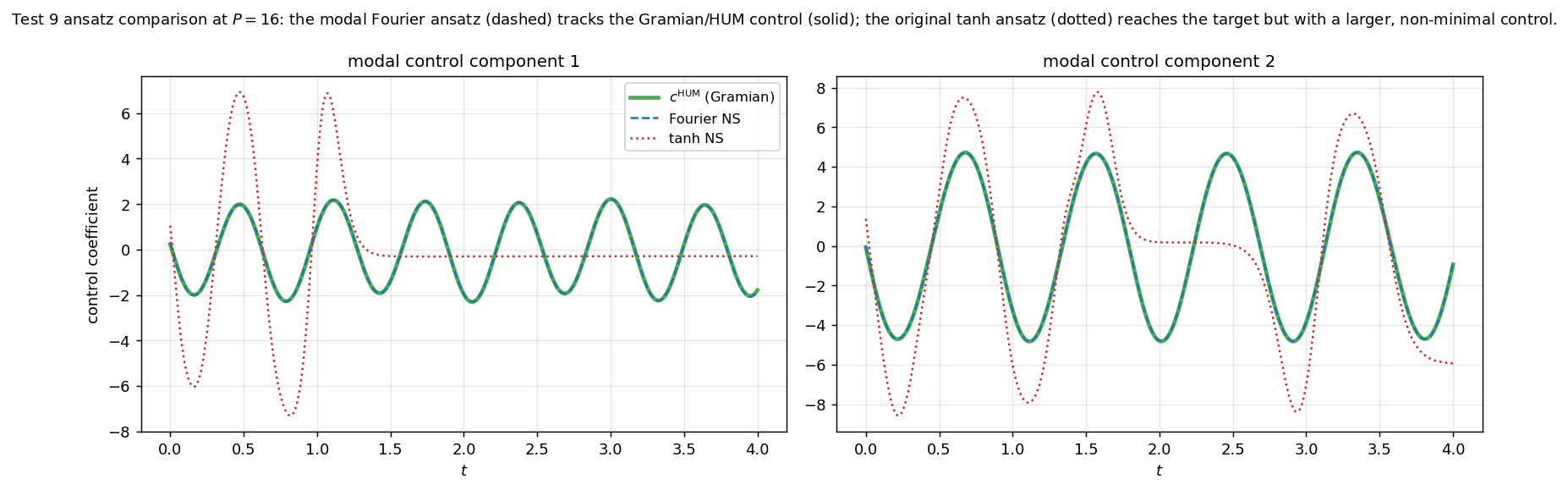
Both variants drive the projected state close to the target, as reflected by their comparable terminal errors. They differ, however, in the control selected by the optimization. In this experiment, the tanh time-network produces an admissible steering control whose trajectory differs substantially from the minimum-energy Gramian/HUM reference. The modal Fourier ansatz incorporates the frequencies \(\sqrt{\mu_k}\) appearing in the propagator \(e^{A_P^T(T-t)}\), and therefore has a much smaller representation error for the reference control in this linear setting. With the same reduced objective, the Fourier-feature version recovers a control much closer to \(c_P^{\textrm{HUM}}\), with a relative control error below \(10^{-2}\).
The Fourier dictionary should therefore be interpreted as a frequency-informed specialization of the Neural-Spectral strategy for the linear wave equation, where the modal time scales are known analytically. It uses the same modal representation of the dynamics and the same reduced control objective, but replaces the generic trainable tanh time-network by a fixed feature map matched to the spectral time scales of the problem.
5 1D Re-indexing of Multi-dimensional Spectrum↩︎
As established in Lemma 1, the spectrum of the operator \(A\) is naturally indexed by pairs \[(k,\sigma)\in(\mathbb{N}^*)^N\times\{+,-\}.\] For the purposes of constructing neural operator approximations, it is convenient to replace this multi-index notation with a one-dimensional enumeration. This avoids notational and dimensional ambiguities when the spectral coefficients are represented as finite input and output vectors. The purpose of this appendix is to prove Lemma 2 by constructing such an explicit enumeration.
We first enumerate \((\mathbb{N}^*)^N\). For each \(k=(k_1,\dots,k_N)\in(\mathbb{N}^*)^N\), define \[s(k):=\sum_{j=1}^N k_j^2\in\mathbb{N}^*.\] For each \(m\in\mathbb{N}^*\), set \[S_m:=\left\{k\in(\mathbb{N}^*)^N:\;s(k)=m\right\}.\] Each set \(S_m\) is finite. Indeed, if \(k\in S_m\), then \[1\le k_j\le \sqrt m, \qquad j=1,\ldots,N.\] Hence, each coordinate \(k_j\) can take at most \(\lfloor\sqrt m\rfloor\) values, and therefore \[|S_m|\le \lfloor\sqrt m\rfloor^N<\infty.\] Moreover, since \(s(k)\in\mathbb{N}^*\) for every \(k\in(\mathbb{N}^*)^N\), we have \(k\in S_{s(k)}\). Thus \[(\mathbb{N}^*)^N=\bigcup_{m=1}^\infty S_m.\] The union is disjoint, because if \(k\in S_m\cap S_\ell\), then \(s(k)=m=\ell\).
For each nonempty set \(S_m\), we order its elements lexicographically and write \[S_m=\left\{k_1^m,k_2^m,\ldots,k_{|S_m|}^m\right\}.\] Define \[n_0:=0, \qquad n_m:=\sum_{\ell=1}^m |S_\ell|, \qquad m\ge1.\] Then \((n_m)_{m\ge0}\) is nondecreasing, and \(n_m\to\infty\) as \(m\to\infty\). To see this, for each \(r\in\mathbb{N}^*\), consider \[k^r:=(r,1,\ldots,1)\in(\mathbb{N}^*)^N.\] These vectors are pairwise distinct and satisfy \[s(k^r)=r^2+(N-1).\] Thus \(S_{r^2+(N-1)}\neq\emptyset\) for infinitely many values of \(r\). Consequently, the partial sums \[n_m=\sum_{\ell=1}^m |S_\ell|\] cannot remain bounded, and hence \(n_m\to\infty\).
We now define a map \[q:\mathbb{N}^*\to(\mathbb{N}^*)^N.\] Given \(j\in\mathbb{N}^*\), since \(n_m\to\infty\), there exists at least one \(m\ge1\) such that \(j\le n_m\). Let \(m\) be the smallest such integer. Then \[n_{m-1}<j\le n_m.\] In particular, \(S_m\neq\emptyset\), and we define \[\label{def:q} q(j):=k^m_{\,j-n_{m-1}}.\tag{57}\] This gives a well-defined map \[q:\mathbb{N}^*\longrightarrow(\mathbb{N}^*)^N, \qquad j\longmapsto q(j).\]
We now prove that \(q\) is a bijection. Suppose first that \(q(j_1)=q(j_2)\). Let \(m_1,m_2\) be the corresponding integers such that \[n_{m_1-1}<j_1\le n_{m_1}, \qquad n_{m_2-1}<j_2\le n_{m_2}.\] Then \[q(j_1)\in S_{m_1}, \qquad q(j_2)\in S_{m_2}.\] Since the sets \(S_m\) are pairwise disjoint and \(q(j_1)=q(j_2)\), we must have \(m_1=m_2\). Within the ordered list of \(S_{m_1}\), the equality \(q(j_1)=q(j_2)\) then implies that the two elements have the same position, namely \[j_1-n_{m_1-1}=j_2-n_{m_1-1}.\] Hence \(j_1=j_2\), and \(q\) is injective.
To prove surjectivity, let \(k\in(\mathbb{N}^*)^N\). Set \(m:=s(k)\). Then \(k\in S_m\), so there exists an index \(r\), with \(1\le r\le |S_m|\), such that \[k=k_r^m.\] By construction, \[q(n_{m-1}+r)=k_r^m=k.\] Therefore \(q\) is surjective. Hence \(q\) is a bijection.
Finally, to incorporate the two branches \(\{+,-\}\), we define \[\kappa:\mathbb{N}^*\to(\mathbb{N}^*)^N\times\{+,-\}\] by \[\kappa(2j-1):=(q(j),+), \qquad \kappa(2j):=(q(j),-), \qquad j\in\mathbb{N}^*.\] Since \(q\) is a bijection, it follows immediately that \(\kappa\) is also a bijection. Indeed, every pair \((k,+)\) is attained by \(2q^{-1}(k)-1\), and every pair \((k,-)\) is attained by \(2q^{-1}(k)\).
Using \(\kappa\), we may re-index the eigenvalues and eigenfunctions of \(A\) by a single integer. For each \(n \in \mathbb{N}^*\), we define \[\begin{align} \lambda_{2n-1}:=\lambda_{q(n)}^{+}, \qquad \lambda_{2n}:=\lambda_{q(n)}^{-} \\ \phi_{2n-1}:=\phi_{q(n)}^{+} \qquad \phi_{2n}:=\phi_{q(n)}^{-}. \end{align}\] Thus, the full spectral family \[\left\{\left(\lambda_k^\pm,\phi_k^\pm\right)\right\}_{k\in(\mathbb{N}^*)^N}\] is equivalently represented as the one-dimensional sequence \[\{(\lambda_n,\phi_n)\}_{n\in\mathbb{N}^*}.\]