Spectral clustering of time-evolving networks using spatio-temporal random walks
January 01, 1970
Abstract
Temporal (or time-evolving) networks provide a natural framework for modeling complex systems with time-dependent interactions, where understanding the evolution of community structures is a central challenge. While random walk-based approaches to community detection in static networks are well established through the spectral analysis of associated transfer operators, extending these ideas to temporal networks is nontrivial due to the inherent time-dependence of the underlying dynamics. In this work, we develop a general framework for community detection in temporal networks that is based on multi-view canonical correlation analysis (mCCA). We show that the proposed formulation admits a spectral characterization via a time-reversible random walk on an augmented space–time network, providing a clear dynamical interpretation of temporal communities as metastable structures of the process. Furthermore, we analyze key spectral properties of the resulting transfer operators and the interplay between spatial and temporal effects, which allows us to distinguish between structural features and artifacts induced by the snapshot coupling. Finally, we derive a reduced-order model, which preserves the essential spectral properties while significantly improving computational efficiency. We show that the proposed approach effectively detects communities in temporal networks and captures their evolution.
Keywords: temporal networks, spectral clustering, community detection, random walks, transfer operators
1 Introduction↩︎
Community detection is one of the central problems in network science. In static networks, spectral methods based on random walks provide a powerful framework for identifying communities as metastable regions of an underlying stochastic process. The key idea is that communities correspond to subsets of nodes between which transitions occur only rarely, resulting in slowly decaying dynamical modes that can be characterized through the spectral properties of associated transfer operators [1]–[6].
Many real-world networks, however, are inherently dynamic. Social interactions, mobility patterns, communication networks, and contact networks relevant for epidemic spreading evolve over time, giving rise to temporal (or time-evolving) networks [7]–[9]. In epidemiological applications, identifying persistent and evolving communities is particularly important, as such structures can strongly influence transmission pathways and the effectiveness of intervention strategies. More generally, however, one seeks to identify communities that persist over extended periods while allowing for structural changes such as community splits, merges, or changes in membership. Extending the dynamical perspective on community detection from static to temporal networks is challenging, since the underlying dynamics are no longer governed by a single transfer operator but by a family of time-dependent operators.
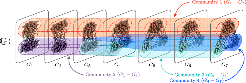
While the notion of a community is well understood in static networks, its extension to temporal networks is considerably more subtle. Time-evolving systems are commonly represented as temporal networks, that is, sequences of graph snapshots that share a common vertex set but exhibit evolving edge structure. From a mathematical perspective, this setting raises several fundamental challenges: how to compare network structure across time, how to define notions of coherence and persistence, how to detect phases of stability during the network evolution, and how to extend spectral methods for community detection from static to temporal networks [10], [11]. The goal is to cluster nodes across network snapshots into coherent groups, that is, subsets of nodes that remain densely connected over extended periods of time, see figure 1.
In this work, we adopt a dynamical perspective on community detection and interpret communities as coherent structures of an underlying random-walk process [1], [3], [4], [12]–[14]. From a network-theoretic perspective, communities are subsets of nodes that are densely connected internally and only sparsely connected to the remainder of the network. Dynamically, they correspond to regions in which a random walker becomes temporarily trapped. Starting from such a region, the probability of remaining within it is high, while transitions to other parts of the network occur only rarely. This behavior is commonly referred to as metastability. More precisely, a random process is metastable if the state space can be partitioned into subsets such that mixing within each subset occurs on a much shorter timescale than transitions between different subsets.
In static networks, this separation of timescales is reflected in the spectral properties of transfer operators associated with the random-walk process [2], [5], [6], [15]. In particular, for time-reversible random walks, the Koopman operator, which describes the evolution of real-valued functions of the nodes (network observables), is self-adjoint with respect to a weighted inner product. This implies a real spectrum and an orthogonal basis of eigenvectors. The dominant eigenvalues close to one correspond to slowly decaying modes of the dynamics. The associated eigenvectors can be interpreted as network observables that are approximately invariant under the action of the Koopman operator and whose level sets partition the nodes into metastable subsets of the underlying random walk, i.e., into communities [1], [3], [13], [16]–[18]. This operator-theoretic viewpoint provides a principled way to detect and interpret community structures via the dynamics of the underlying random-walk process.
Here, we study the evolution of communities in temporal networks in the same manner, where the process now propagates across snapshots according to the underlying network structure. However, extending the dynamical perspective on community detection from static to temporal networks is non-trivial. Dynamical processes on networks whose structure changes over time are time-dependent and are therefore described by a whole family of Koopman operators. As a consequence, the rich set of tools developed for community detection in static networks is not directly applicable in the temporal setting. Early approaches to community detection in temporal networks proceed by detecting communities independently within each snapshot and matching them across time [10], [19]. However, such methods face several fundamental challenges, including the ambiguity of community labels, the instability of static community detection algorithms, which may produce significantly different partitions even under minor or no changes in the network [20], as well as the dependence on ad hoc matching procedures and parameter tuning.
In this paper, we turn to Canonical Correlation Analysis (CCA), a procedure that aims to find linear transformations of random variables that maximize the correlation between them [21]. We note that the computation of dominant eigenvectors of transfer operators associated with static networks can be reformulated as an instance of CCA, in which one seeks to maximize the correlation between observables at different time steps of the random process [18]. We build on the extension of this approach proposed in [22], where a generalization of CCA, known as multi-view CCA [23], is employed. A temporal network is represented as a sequence of static networks (snapshots), for example obtained by “freezing” the structure of the temporal network at equally spaced time intervals with a desired frequency. Multi-view CCA is then used to maximize a weighted correlation between observables across adjacent snapshots whose level sets are later used to cluster nodes from different snapshots into communities that persist over time. We extend this framework by introducing a general coupling scheme that allows for incorporating correlations between arbitrary pairs of snapshots with different relative weights into the overall objective function. This leads to a more robust method that is more resilient to noisy fluctuations and reduces the emergence of highly correlated observables across snapshots whose level sets do not correspond to meaningful temporal communities. Moreover, this approach enables flexible adaptation to different application scenarios, while preserving the underlying framework. For instance, one can explore whether the data exhibits periodic behavior through a cyclic coupling of the last snapshots of the temporal network to the first snapshots.
The multi-view CCA approach enables us not only to detect sets of nodes that remain densely interconnected over longer time periods, but also to capture changes in community structure throughout the evolution. In contrast to classical CCA, which correlates only two selected time points, this method incorporates the full temporal information and thus retains insight into intermediate structural changes that would otherwise remain invisible when considering only particular time points, such as the beginning and the end of the network evolution.
We show that the multi-view CCA approach with a general coupling scheme reduces to the analysis of spectral properties of a time-reversible random walk on a static network defined on an augmented node set, whose structure encodes both the spatial organization of the temporal network at different time points and the temporal ordering of snapshots. In this representation, a random walker can move not only in space (between nodes) but also through time (between snapshots), which naturally connects our approach to community detection methods for static networks and provides a clear and intuitive interpretation of temporal communities as coherent sets of the associated spatio-temporal random walk.
Our perspective is related to a common approach in the literature, where temporal networks are represented as space–time (multilayer) networks by introducing inter-snapshot edges [24], and random processes on such augmented networks are analyzed. In many constructions, only identical nodes are connected across snapshots, typically with uniform inter-snapshot weights [24]–[26], and connections are often restricted to consecutive snapshots [27]. As a result, the chain-like geometry of the snapshot coupling scheme gives rise to slowly decaying modes, which may be misinterpreted as metastable behavior even in the absence of any intrinsic community structure. Some models allow connections between different nodes across snapshots, but they either rely entirely on user-defined parameters [28] or disregard the temporal ordering of snapshots, thereby identifying communities in an aggregated network rather than over contiguous time intervals [29]. In contrast, the space–time network induced by the snapshot coupling and the structure of the temporal network provides a more principled construction. The weights of inter-snapshot connections are determined by the structure of the snapshots themselves and modulated by a flexible notion of temporal proximity. This allows us to simultaneously capture structural and temporal relationships, while at the same time controlling and reducing spurious metastability effects arising from the geometry of the coupling scheme.
The key observation of this paper is that a broad class of multi-view CCA formulations for temporal community detection is equivalent to the spectral analysis of a reversible Markov process on an augmented space-time network. This equivalence enables a rigorous analysis of temporal communities using transfer-operator techniques and provides a principled framework for distinguishing genuine structural features from artifacts induced by temporal coupling.
Our main contributions are threefold:
First, we derive a general multi-view CCA model for temporal networks based on Perron–Frobenius and Koopman operators and show that this formulation reduces to a generalized eigenvalue problem. Moreover, we establish a connection to a random walk on an augmented static network representing the original temporal network. This perspective complements existing notions of spatio-temporal random walks on temporal networks.
Second, we analyze the spectral properties of the resulting spatio-temporal dynamics and investigate how temporal effects induced by the snapshot coupling interact with spatial effects arising from the network structure. A principled interpretation of the associated eigenvalues and eigenvectors has largely been missing in the literature, yet is essential for separating spatial and temporal contributions, that is, for distinguishing between effects that arise purely from the coupling mechanism and those that encode meaningful structural events such as community splits, merges, or changes in community membership.
Lastly, we derive a reduced model of the spatio-temporal random walk for community structure analysis. We prove that the aforementioned spectral properties transfer to the projected setting under mild conditions and show that the resulting reduced model remains effective in practice. Since the dimensionality of the full model grows quadratically with both the number of nodes and the number of snapshots, computations quickly become expensive even for moderately large datasets, making this reduction a natural and useful extension. In addition, we provide spectral error bounds that quantify the accuracy of the reduced representation.
We first introduce the necessary theoretical background on random walks and transfer operators in section 2. We then develop the multi-view CCA framework and analyze its spectral properties in section 3. We present the reduced-order modeling approach and numerical results in sections 4 and 5. Finally, we provide a brief conclusion and suggest directions for future research in section 6.
2 Theoretical background↩︎
In this section, we provide a brief overview of the required concepts. Let \(\mathbb{G} = (G_1, \dots, G_M)\) be a temporal network defined over an observation period partitioned into \(M\) discrete time steps. Each index \(t \in \{1, \dots, M\}\) corresponds to a static snapshot \(G_t = (V, E_t, \omega_t)\). In this formulation, the node set \(V = \{v_1, \dots, v_N\}\) is fixed across all snapshots, the edge set \(E_t \subseteq V\times V\) represents the undirected interactions occurring during time step \(t\), and \(\omega_t: E_t\rightarrow\mathbb{R}\) denotes a symmetric function assigning weights to the edges of \(G_t\). The (weighted) degree of node \(v_i\) of \(G_t\) is given by \[\deg_t(v_i) = \sum_{j=1}^N \omega_t(v_i,v_j),\] and the corresponding diagonal degree matrix is defined by \[D_t = \operatorname{diag}(\deg_t(v_1), \dots, \deg_t(v_N)).\]
2.1 Random walks on temporal networks↩︎
On a static network, a standard random walk process is defined as a discrete-time Markov chain that moves between adjacent nodes, where the transition probabilities are proportional to the edge weights. Since the edge set is fixed, the transition rules do not depend on time but only on the current state of the process. We extend this notion from static to temporal networks and consider a random process \(\{X_t\}_{t=1}^M\) evolving across the snapshots of a temporal network \(\mathbb{G}\).
Let \(A_t\in\mathbb{R}^{N\times N}\) denote the weighted adjacency matrix of \(G_t\) where \((A_t)_{ij}=\omega_t(v_i,v_j)\). Each snapshot \(G_t\) induces its own transition matrix \[\label{eq:transition95matrix} S_t = D_t^{-1} A_t,\tag{1}\] which governs the random walk dynamics within that snapshot. Starting in snapshot \(G_1\), the process evolves forward in time by moving to the next snapshot at each time step and following the transition rules determined by the transition matrix \(S_t\) at time \(t\). As a consequence, the resulting process is in general time-inhomogeneous and may no longer be reversible. Therefore, many classical methods for community detection developed for static networks are not directly applicable in this setting. Nevertheless, the underlying intuition remains similar. Although edges in a temporal network may appear or disappear over different snapshots, if a subset of nodes remains densely connected (coherent) throughout the network’s evolution, then a random walk process starting in this region will with high probability remain confined to it for as long as this structure persists. This observation is consistent with the interpretation of communities as metastable sets of random processes in static networks.
In what follows, we adopt a transfer operator perspective on network dynamics and extend it from static to temporal networks.
Definition 1 (Observables and probability distributions). Let \[\mathbb{U} = \{ f \mid f \colon V \to \mathbb{R} \}\] denote the space of real-valued functions defined on the node set \(V\). A function \(\rho \in \mathbb{U}\) is called a probability distribution* if \(\rho(v_i) \ge 0\), for all \(i = 1, \dots, N\), and \[\sum_{i=1}^{N} \rho(v_i) = 1.\] In general, functions \(f\in\mathbb{U}\) are referred to as network observables.*
Definition 2 (Standard and weighted inner products). Let \(f,g \in \mathbb{U}\) be two network observables. The standard inner product on \(\mathbb{U}\) is given by \[\langle f, g \rangle = \sum_{i=1}^{N} f(v_i)\, g(v_i).\] Given a probability distribution \(\mu\), the corresponding \(\mu\)-weighted inner product on \(\mathbb{U}\) is defined by \[\langle f, g \rangle_{\mu} = \sum_{i=1}^{N} f(v_i)\, g(v_i)\, \mu(v_i).\]
Analogously to random processes on static networks, the dynamics of the random process \(\{X_t\}_{t=1}^M\) on a temporal network can be described from two dual perspectives: through the evolution of its probability distributions and through the evolution of network observables across time snapshots [30]. For distinct time points \(t\) and \(s\) with \(t < s\), we now define two transfer operators.
Definition 3 (Multi step Perron–Frobenius and Koopman operators). Let \(\rho \in \mathbb{U}\) be a probability distribution and let \(f\in\mathbb{U}\) be a network observable. Let \(S_{ts}=S_tS_{t+1}\cdots S_{s-1}\) for \(t<s\), where the entry \((S_{ts})_{ij}\) is the probability that a random walker starting in node \(v_i\) at time \(t\) will end up in node \(v_j\) at time \(s\).
The multi step Perron–Frobenius operator* between times \(t\) and \(s\), denoted by \(\mathcal{P}_{ts} \colon \mathbb{U} \rightarrow \mathbb{U}\), is defined by \[\mathcal{P}_{ts} \rho(v_i)=\sum_{j=1}^N (S_{ts})_{ji} \, \rho(v_j).\]*
The multi step Koopman operator* between times \(t\) and \(s\), denoted by \(\mathcal{K}_{ts} \colon \mathbb{U} \rightarrow \mathbb{U}\), is defined by \[\mathcal{K}_{ts} f(v_i) = \sum_{j=1}^N (S_{ts})_{ij} f(v_j)=\mathbb{E}[f(X_{s})\mid X_t=v_i].\]*
Matrix representations \(P_{ts} \in \mathbb{R}^{N\times N}\) and \(K_{ts} \in \mathbb{R}^{N\times N}\) of the operators \(\mathcal{P}_{ts}\) and \(\mathcal{K}_{ts}\), respectively, are given by \[\label{eq:koopman95mat95rep} P_{ts} = S_{ts}^{\top} \quad\text{and}\quad K_{ts} = S_{ts}.\tag{2}\] Suppose the ensemble of random walkers is initialized on the first snapshot \(G_1\) with probability distribution \(\mu_1\). The evolution of probability distributions is then given by \[\label{eq:evolution95of95prob95distr} \mu_{s} = \mathcal{P}_{ts} \mu_t,\tag{3}\] where \(\mu_t\) and \(\mu_s\) denote the probability distributions of the process at times \(t\) and \(s\) (on snapshots \(G_t\) and \(G_s\)). On the level of observables, the dynamics are described by the family of Koopman operators \(\mathcal{K}_{ts}\). Applied to an observable \(f\) at time \(t\), the operator \(\mathcal{K}_{ts}\) propagates it \(s-t\) steps forward according to the random walk dynamics between times \(t\) and \(s\) and computes its expected values at the network nodes at time \(s\). We now introduce a reweighted Perron–Frobenius operator that propagates observables from time \(t\) to time \(s\) with respect to the reference distributions \(\mu_t\) and \(\mu_s\).
Definition 4 (Multi step Reweighted Perron–Frobenius operator). Let \(u \in \mathbb{U}\) and let \(S_{ts} = S_t S_{t+1} \cdots S_{s-1}\) for \(t < s\). Let \(\mu_t\), \(1 \le t \le M\), denote the probability distributions of the random process on the temporal network at time \(t\). The multi step reweighted Perron–Frobenius operator* between times \(t\) and \(s\), denoted by \(\mathcal{T}_{ts} : \mathbb{U} \to \mathbb{U}\), is defined by \[\mathcal{T}_{ts} u(v_i) = \frac{1}{\mu_s(v_i)} \sum_{j=1}^{N} (S_{ts})_{ji} \, \mu_t(v_j) \, u(v_j) = \mathbb{E}[u(X_t) \mid X_s = v_i].\]*
Let \(\boldsymbol{\mu}_t=[\mu_t(v_1),\dots,\mu_t(v_N)]^{\top}\) denote the vector representation of the probability distribution \(\mu_t\), and let \(D_{\mu_t} = \operatorname{diag}(\boldsymbol{\mu}_t)\). The matrix representation of the reweighted Perron–Frobenius operator \(T_{ts} \in \mathbb{R}^{N \times N}\) is given by \[\label{eq:reweighted95perron95frobenius95mat95rep} T_{ts} = D_{\mu_s}^{-1} (S_{ts})^\top D_{\mu_t}.\tag{4}\]
The operators \(\mathcal{K}_{ts}\) and \(\mathcal{T}_{ts}\) (and their respective matrix representations \(K_{ts}\) and \(T_{ts}\)) are adjoint with respect to the inner products induced by the probability distributions \(\mu_t\) and \(\mu_s\), that is, \[\langle f, \mathcal{K}_{ts} g\rangle_{\mu_t}=\langle\mathcal{T}_{ts} f,g\rangle_{\mu_{s}}.\]
Remark 1. Definitions 3 and 4 generalize the standard Perron–Frobenius and Koopman operators for discrete-time dynamics [5], which describe the one-step propagation of probability distributions and observables and can be recovered from our definition by \(s=t+1\). In [22], such one-step operators were used to model propagation only between consecutive snapshots. Here, we additionally introduce operators that characterize propagation across multiple snapshots.
3 Community detection in temporal networks↩︎
Guided by the intuition from the static network case, we seek observables for each snapshot that remain highly correlated under the underlying random-walk process. More precisely, the goal is to identify observables that preserve information about the coherent behavior of the time-inhomogeneous random walk, such that their level sets partition the nodes across all snapshots into communities that persist over time. This perspective naturally leads to a multi-view extension of the CCA formulation [23], where we look for a collection of observables \(f_t\) for \(1 \le t \le M\) (i.e., one observable for each snapshot), that maximize a weighted correlation between the random variables \(f_1(X_1), \dots, f_M(X_M)\). In this section, we formalize this idea and begin by defining correlations between network observables at different snapshots.
3.1 Multi-view canonical correlation analysis (mCCA)↩︎
To quantify and maximize temporal correlations, we introduce covariance and cross-covariance operators associated with the underlying random process. Building on [18], [22], we generalize the notion of cross-covariance by defining it between arbitrary time points \(t\) and \(s\).
Definition 5 (Covariance and cross-covariance operators). Let \(f_t \in \mathbb{U}\), with \(1\le t\le M\), denote a network observable for the snapshot \(G_t\). Let \(\mu_t\) be the probability distribution at time \(t\) and let \(S_{ts}\) denote the transition probability matrix from time \(t\) to time \(s\) as given in definition 3.
The covariance operator* at time \(t\), \(\mathcal{C}_{tt} \colon \mathbb{U} \rightarrow \mathbb{U}\), is defined as \[\mathcal{C}_{tt} f_t(v_i) = \mu_t(v_i) f_t(v_i).\]*
The cross-covariance operator* between times \(t\) and \(s\) for \(t<s\), \(\mathcal{C}_{ts} \colon \mathbb{U} \rightarrow \mathbb{U}\), is defined as \[\mathcal{C}_{ts} f_s(v_i) = \sum_{j=1}^N \mu_t(v_i) (S_{ts})_{ij} f_s(v_j).\]*
We can now express the covariance of an observable \(f_t\) at time \(t\) as \[\langle f_t, \operatorname{\mathcal{C}}_{tt} f_t \rangle = \sum_{i=1}^N \mu_t(v_i) f_t(v_i)^2 = \mathbb{E}_{\mu_t}[f_t(X_t)^2] = \operatorname{var}(f_t)\] and the cross-covariance of the observables \(f_t\) and \(f_s\) at times \(t\) and \(s\) as \[\langle f_t, \operatorname{\mathcal{C}}_{ts} f_s \rangle = \sum_{i=1}^N \sum_{j=1}^N f_t(v_i)\,\mu_t(v_i)\,(S_{ts})_{ij}\,f_s(v_j) = \mathbb{E}_{\mu_{ts}} \big[ f_t(X_t) f_s(X_{s}) \big] = \operatorname{cov}(f_t,f_s),\] where \(\mu_{ts}(v_i,v_j) = \mathbb{P}(X_t = v_i,\, X_{s} = v_j) = \mu_t(v_i)\, (S_{ts})_{ij}\) is the joint probability distribution of the random process at times \(t\) and \(s\).
Let \(\mathbf{f}_t\) and \(\mathbf{f}_s\) denote the vector representations of the observables \(f_t\) and \(f_s\) for \(t<s\) and let \(C_{tt}\) and \(C_{ts}\) be the matrix representations of the operators \(\mathcal{C}_{tt}\) and \(\mathcal{C}_{ts}\). Then \[\operatorname{var}(f_t) = \langle \mathbf{f}_t, C_{tt}\mathbf{f}_t\rangle = \mathbf{f}_t^\top C_{tt}\mathbf{f}_t \quad \text{and} \quad \operatorname{cov}(f_t,f_s) = \langle \mathbf{f}_t, C_{ts}\mathbf{f}_s\rangle = \mathbf{f}_t^\top C_{ts}\mathbf{f}_s.\] The correlation between observables \(f_t\) and \(f_s\) is therefore given by \[\label{eq:correlation} \operatorname{corr}(f_t,f_s) = \frac{\mathbf{f}_t^\top C_{ts}\mathbf{f}_s}{\sqrt{\mathbf{f}_t^\top C_{tt}\mathbf{f}_t}\, \sqrt{\mathbf{f}_s^\top C_{ss}\mathbf{f}_s}}.\tag{5}\] Our objective is to maximize the weighted correlation across all snapshots \[\label{eq:weighted95correlation} \max_{f_t\in\mathbb{U}} \sum_{\substack{t,s=1 \\ t < s}}^{M} w_{ts} \, \operatorname{corr}(f_t, f_{s}),\tag{6}\] where \(w_{ts}\ge0\), for \(1\le t<s\le M\), are coupling weights that quantify the importance of the correlation between observables at times \(t\) and \(s\). Although only the weights with \(t<s\) enter the objective function 6 , we extend them for convenience to all pairs of indices by defining \(w_{st}=w_{ts}\) and \(w_{tt}=0\). This convention simplifies several expressions and derivations below. Since our aim is to identify temporal communities and detect events corresponding to structural changes, the coupling weights should encode temporal proximity: snapshots that are close in time should be coupled with higher weights, while those farther apart receive progressively lower weights. As persistent communities are characterized by stability over longer periods, coupling only consecutive snapshots may therefore make the solutions of 6 sensitive to short-term fluctuations and noise. By coupling observables across longer time intervals, we obtain more robust and temporally consistent solutions. Furthermore, depending on the application, alternative snapshot coupling schemes may be more appropriate, e.g. couplings between temporally distant snapshots can be used to reveal recurring or periodic community patterns. We will illustrate these effects through numerical examples in section 5.
Since the correlation 5 is invariant under scalar multiplication of observables, i.e., \[\operatorname{corr}(f_t,f_s)=\operatorname{corr}(a f_t,b f_s) \quad \text{for all } a,b\in\mathbb{R},\] we may assume, without loss of generality, that all observables \(f_t\), with \(1\le t\le M\), satisfy \(\operatorname{var}(f_t)=1\). We can then rewrite 6 in the form \[\label{eq:maximization95problem} \max_{\mathbf{f}_t}\sum_{\substack{t,s=1 \\ t < s}}^{M}w_{ts}\mathbf{f}_t^\top C_{ts}\mathbf{f}_{s} \text{ s.t.}\mathbf{f}_t^\top C_{tt}\mathbf{f}_t=1, \text{ for all } t=1,...,M.\tag{7}\] Following the approach from [22], we use Lagrange multipliers to solve this optimization problem, resulting in \[\mathcal{L}(\mathbf{f}_1,\lambda_1,...,\mathbf{f}_M,\lambda_M)=\sum_{\substack{t,s=1 \\ t < s}}^{M}w_{ts}\mathbf{f}_t^\top C_{ts}\mathbf{f}_s -\sum_{t=1}^{M}\frac{r_t}{2}\lambda_t(\mathbf{f}_t^\top C_{tt}\mathbf{f}_t-1),\] where we rescale each Lagrange multiplier \(\lambda_t\) by the factor \(\frac{r_t}{2}\), with \(r_t=\sum_{s=1}^{M} w_{ts}\). Here, \(r_t\) serves as a normalization factor that accounts for the total weight assigned to snapshot \(G_t\), while the factor \(\frac{1}{2}\) cancels out when differentiating the quadratic term, which simplifies the subsequent computations.
For any observables \(\mathbf{f}_1,\dots,\mathbf{f}_M\) that solve 7 , the condition \(\partial_{\mathbf{f}_t}\mathcal{L} = 0\) must hold for all \(1\le t\le M\). Taking derivatives of the Lagrangian function with respect to \(\mathbf{f}_1,\dots,\mathbf{f}_M\), and using \(w_{ts}=w_{st}\) we obtain the equations \[\label{eq:derivatives} \begin{align} \partial_{\mathbf{f}_1}\mathcal{L}&= w_{12} C_{12}\mathbf{f}_2+w_{13}C_{13}\mathbf{f}_3+\dots+w_{1M}C_{1M}\mathbf{f}_M-r_1\lambda_1C_{11}\mathbf{f}_1=0,\\ \partial_{\mathbf{f}_2}\mathcal{L}&= w_{21} C_{12}^\top\mathbf{f}_1+ w_{23} C_{23}\mathbf{f}_3+\dots+w_{2M}C_{2M}\mathbf{f}_M-r_2\lambda_2C_{22}\mathbf{f}_2=0,\\ \vdots\\ \partial_{\mathbf{f}_M}\mathcal{L}&= w_{M1}C_{1M}^\top\mathbf{f}_1 + w_{M2}C_{2M}^\top \mathbf{f}_2+\cdots+w_{M(M-1)}C_{(M-1)M}^\top\mathbf{f}_{M-1}-r_M\lambda_MC_{MM}\mathbf{f}_M=0. \end{align}\tag{8}\]
Allowing independent multipliers \(\lambda_t\) would lead to a multiparameter eigenvalue problem [31], [32]. Such problems fall outside classical spectral theory and typically require more advanced analytical and numerical techniques. While this would be an interesting direction for future research, it is beyond the scope of the present work.
In what follows, we assume that \(\lambda_t = \lambda\) for all \(t=1,\dots,M\), which allows us to rewrite the system in the form of a generalized eigenvalue problem. We introduce the snapshot coupling matrix \(H=[h_{ts}]\in\mathbb{R}^{M\times M}\) containing the normalized coupling weights between snapshots \[\label{eq:compute95H} h_{ts} = \frac{w_{ts}}{r_t}, \qquad 1 \le t,s \le M .\tag{9}\] For each \(t\), dividing the corresponding equation in 8 by \(r_t\) and rewriting the system in matrix form, we obtain \[\label{eq:generalized95eigval95problem} \mathbf{A}_H \mathbf{f}= \lambda \mathbf{B}\mathbf{f},\tag{10}\] where \[\mathbf{A}_H = \begin{bmatrix} 0 & h_{12}C_{12} & \cdots & h_{1M}C_{1M} \\ h_{21}C_{12}^{\top} & 0 & \ddots & \vdots\\ \vdots & \ddots & \ddots & h_{(M-1)M}C_{(M-1)M} \\ h_{M1}C_{1M}^\top & \cdots & h_{M(M-1)}C_{(M-1)M}^{\top} & 0 \end{bmatrix},\] \[\mathbf{B}= \begin{bmatrix} C_{11} & 0 & \cdots & 0 \\ 0 & C_{22} & \ddots & \vdots \\ \vdots & \ddots & \ddots & 0 \\ 0 & \cdots & 0 & C_{MM} \end{bmatrix} \,\,\, \text{and} \,\,\, \mathbf{f}= \begin{bmatrix} \mathbf{f}_1\\ \mathbf{f}_2\\ \vdots\\ \mathbf{f}_M \end{bmatrix}.\] From definition 5, the matrix representations of the covariance and cross-covariance operators are given by \[C_{tt} = D_{\mu_t} \quad \text{and} \quad C_{ts} = D_{\mu_t} S_{ts}.\] Defining \(\mathbf{C}_H=\mathbf{B}^{-1}\mathbf{A}_H\), and using 2 and 4 , we obtain
\[\label{eq:k95pf95notation} \mathbf{C}_H= \begin{bmatrix} 0 & h_{12}K_{12} & \cdots & h_{1M}K_{1M}\\ h_{21}T_{12} & 0 & \ddots & \vdots \\ \vdots & \ddots & \ddots & h_{(M-1)M}K_{(M-1)M}\\ h_{M1}T_{1M} & \dots & h_{M(M-1)}T_{(M-1)M} & 0 \end{bmatrix}\tag{11}\]
so that 10 reduces to the standard eigenvalue problem \[\mathbf{C}_H \mathbf{f}= \lambda \mathbf{f}.\]
We can interpret the matrix \(\mathbf{C}_H\) from a transfer-operator perspective. In the standard theory of (one-step) transfer operators in discrete-time dynamics (see remark 1), the Koopman operator evaluates an observable at the current state by taking the conditional expectation of its value at the next state. In this sense, it effectively pulls future information back to the present and is therefore often referred to as a pull-back operator. In contrast, the reweighted Perron–Frobenius operator propagates information forward in time by determining the values of an observable at the next state from its values at the current state. It thus transports information forward along the dynamics and is commonly referred to as a push-forward operator. These interpretations naturally extend to the multi-step transfer operators introduced here. Acting blockwise with \(\mathbf{C}_H\) on \(\mathbf{f}\), the \(t\)th segment of size \(N\) of \(\mathbf{C}_H\mathbf{f}\) is given by \[(\mathbf{C}_H \mathbf{f})_t = \sum_{s=1}^{t-1} h_{ts}\, T_{st}\mathbf{f}_s + \sum_{s=t+1}^{M} h_{ts}\, K_{ts}\mathbf{f}_s,\] i.e., the observable \(\mathbf{f}_t\) is transformed into a weighted average of pushed-forward and pulled-back observables from different times, transported to time \(t\). Therefore, eigenvectors of \(\mathbf{C}_H\) corresponding to large eigenvalues represent observables that are closest to being invariant under the time-inhomogeneous random process described in section 2. The relative contribution of past and future snapshots to \(\mathbf{f}_t\) is given by the coupling matrix \(H\).
3.2 Spatio-temporal random walk↩︎
In this section, we study properties of the matrices \(H\) and \(\mathbf{C}_H\) and relate them to random walks between snapshots and on the augmented space–time network. Proofs of all the lemmas stated in this section are provided in appendix 7.
Definition 6. We define the snapshot coupling network* to be an undirected weighted network \(G_H = (V_H, E_H, \omega_H)\), with the set of nodes \(V_H = \{1,\dots,M\}\), the set of edges \(E_H \subset V_H \times V_H\) such that \((t,s)\in E_H\) if and only if \(w_{ts} \neq 0\) for any \(1 \le t < s \le M\) and the symmetric edge-weight function is given by \(\omega_H(t,s)=w_{ts}\).*
Lemma 1. Let \(H\) be the coupling matrix defined in 9 . Then, there exists a probability distribution \(\boldsymbol{\pi}\in \mathbb{R}^M\) such that the detailed balance condition \[D_{\pi} H = H^{\top} D_{\pi}\] holds, where \(D_{\pi} = \operatorname{diag}(\boldsymbol{\pi})\). Consequently, \(H\) is the transition matrix of a time-reversible random walk on the coupling network \(G_H\). In particular, if \(G_H\) is connected, then \(\boldsymbol{\pi}\) is unique.
The network \(G_H\) can be interpreted as a network defined on the snapshots of the temporal network \(\mathbb{G}\), with edge weights given by the snapshot coupling weights \(w_{ts}\). Based on the previous lemma, \(H\) is thus the transition matrix of the associated random walk on the network \(G_H\).
Lemma 2. The matrix \(\mathbf{C}_H\) is row-stochastic. In particular, its spectral radius satisfies \[\rho(\mathbf{C}_H) = 1.\]
Using this result, we can interpret the matrix \(\mathbf{C}_H\) as the transition matrix of a random walk on an augmented state space, where transitions between snapshots both forward and backward in time are possible. Since this process simultaneously captures transitions across nodes (space) and across snapshots (time), we refer to it as a spatio-temporal random walk, defined on the augmented network described in definition 7. Similar space–time formulations have been used in transfer-operator approaches to coherent-set detection, where coherent sets are identified through the spectral analysis of a process on an augmented space–time domain [33].
Definition 7. The space–time network* \(\mathscr G_H\) is defined on the augmented node set \(V \times \{1,\dots,M\}\), so that it has \(MN\) nodes in total. Each node is given by a pair \((v_i,t)\), where \(1 \le i \le N\) corresponds to a node of \(G_t\). Edges connect nodes \((v_i,t)\) and \((v_j,s)\) between snapshots \(G_t\) and \(G_s\) with nonzero weights if and only if the transition probability between them, given by \(\mathbf{C}_H\), is positive.*
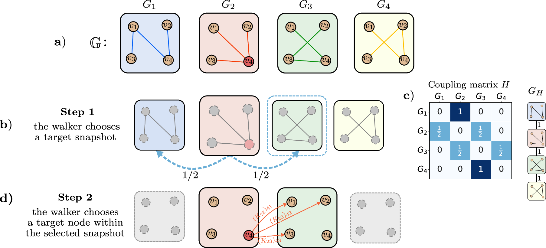
We will use the terms spatio-temporal random walk on a temporal network and on its associated space–time network interchangeably. A formal definition of \(\mathscr G_H\) and further details are given in lemma 8 in appendix 8. An illustration describing the dynamics of the spatio-temporal random walk for a simple temporal network is shown in figure 2, following the structure of \(\mathbf{C}_H\) given in 11 . Starting from a node \(v_i\) at snapshot \(G_t\) (marked in red in figure 2a for \(t=2\)), the walker first selects a target snapshot \(G_s\) (figure 2b) according to the coupling matrix \(H\), that is, according to a random-walk process on the coupling network \(G_H\) (figure 2c). Then, it moves to a node within the chosen snapshot according to the transition probabilities given by \(K_{ts}\) or \(T_{ts}\) depending on the choice of \(s\) (figure 2d). If \(t<s\), the spatial transition is governed by the multi-step transition matrices \(K_{ts}\), corresponding to the forward propagation of the network observables. If \(t > s\), it is governed by \(T_{ts}\), the adjoint of the former, which also admits the interpretation of backward propagation of observables with respect to the time-inhomogeneous process \(\{X_t\}_{t=1}^M\) introduced in section 2.1. The spatio-temporal random walk can therefore be decomposed into two components: a temporal component governed by the transition matrix \(H\) describing transitions between snapshots, and a spatial component governed by the transition matrices \(K_{ts}\) or \(T_{ts}\) describing transitions between nodes. We formalize this decomposition in lemma 7 in appendix 7.
The following lemma additionally shows that the spatio-temporal random walk is time-reversible, allowing us to apply existing results to further investigate its properties in section 3.3.
Lemma 3. There exists a stationary distribution \(\boldsymbol{\nu}\in \mathbb{R}^{MN}\) of the random-walk process on \(\mathscr G_H\) induced by \(\mathbf{C}_H\). Moreover, the process is time-reversible with respect to \(\boldsymbol{\nu}\), that is, the detailed balance condition \[D_{\nu}\mathbf{C}_H = \mathbf{C}_H^{\top} D_{\nu}\] holds, where \(D_{\nu}=\operatorname{diag}(\boldsymbol{\nu})\). Consequently, \(\mathbf{C}_H\) is self-adjoint with respect to the \(\boldsymbol{\nu}\)-weighted inner product. All eigenvalues of \(\mathbf{C}_H\) are real and lie in the interval \([-1,1]\).
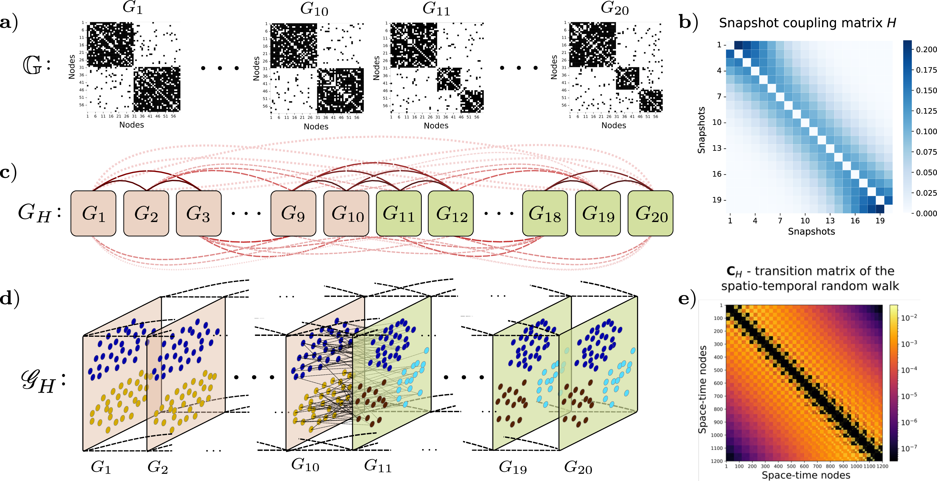
Example 1. Let us consider a temporal network \(\mathbb{G} = (G_1, \dots, G_{20})\) consisting of 60 nodes observed over 20 snapshots, see figure 3. Each snapshot is generated independently from a stochastic block model (SBM), where the within-community and between-community connection probabilities are \(p_{\mathrm{in}} = 0.7\) and \(p_{\mathrm{out}} = 0.05\), respectively. In snapshots \(G_1, \dots, G_{10}\), the network exhibits two communities of equal size (30 nodes each). At snapshot \(G_{11}\), one of these communities splits into two, and this three-community structure persists for the remaining time. The adjacency matrices of the snapshots are shown in figure 3a. In this example, the coupling network \(G_H\) (figure 3c) is chosen such that the edge weights between the snapshots \(G_t\) and \(G_s\) are given by \[\label{eq:decay95coupling} w_{ts} = e^{-\alpha (s-t)^2},\qquad{(1)}\] where \(\alpha > 0\) is a decay parameter that controls how fast the strength of the connection between snapshots decreases with their temporal distance. We set \(\alpha = 0.03\). The corresponding coupling matrix \(H\) is defined as the transition matrix of a random walk on \(G_H\) (figure 3b). We then construct the associated space–time network \(\mathscr G_H\) (figure 3d). A random walker on this network moves between nodes in different snapshots according to the spatio-temporal transition matrix \(\mathbf{C}_H\) (figure 3e).
3.3 Spectral clustering of temporal networks↩︎
Motivated by well-established spectral clustering techniques for community detection in static networks [6], [15], we analyze the spectral properties of the spatio-temporal transition operator \(\mathbf{C}_H\) to identify coherent sets of nodes that persist as densely intraconnected communities over extended time intervals.
In contrast to the purely static setting, eigenvectors of \(\mathbf{C}_H\) may encode two qualitatively different effects: those induced by the temporal coupling between snapshots, and those arising from the internal structure of the individual network snapshots. In [22], [26], these effects are analyzed by visually inspecting the leading eigenvectors of the random walk on the space–time network. Our aim is to provide a more principled theoretical understanding and to disentangle the two contributions. To this end, analogously to definition 1, we define the space–time observable space by \[\mathbb{U}^M=\{f: V \times \{1,\dots,M\} \to \mathbb{R}\}\mid f(\cdot,t)=f_t\in\mathbb{U} \text{ for all }1\le t\le M\}.\] The vector representation of \(f\in\mathbb{U}^M\) is given by \(\mathbf{f}= [\mathbf{f}_1^\top, \mathbf{f}_2^\top, \dots, \mathbf{f}_M^\top]^\top\in\mathbb{R}^{MN}\) and we refer to each observable \(\mathbf{f}_t\in\mathbb{R}^N\) as the \(t\)th snapshot segment of \(\mathbf{f}\). We now introduce a snapshot segment averaging operator \(\mathbf{\Pi}_{\mathrm{avg}} \colon \mathbb{U^M} \to \mathbb{U^M}\), which collapses node-level information within snapshot \(G_t\) to its \(\boldsymbol{\mu}_t\)-weighted mean: \[\label{eq:Pi95avg} \begin{align} \mathbf{\Pi}_{\mathrm{avg}} : (\mathbf{f}_1^\top,\dots,\mathbf{f}_M^\top) \;\mapsto\; \big( \langle \mathbf{f}_1,\mathbf{1}\rangle_{\mu_1}\mathbf{1}^\top,\dots, \langle \mathbf{f}_M,\mathbf{1}\rangle_{\mu_M}\mathbf{1}^\top \big) = \big( \mathbb{E}_{\mu_1}[\mathbf{f}_1]\mathbf{1}^\top,\dots, \mathbb{E}_{\mu_M}[\mathbf{f}_M]\mathbf{1}^\top \big). \end{align}\tag{12}\] The matrix representation of \(\mathbf{\Pi}_{\mathrm{avg}}\) is given by \[\label{eq:Pi95avg95matrix} \mathbf{\Pi}_{\mathrm{avg}}=\operatorname{diag}(\mathbf{1}\boldsymbol{\mu}_1^{\top},\dots,\mathbf{1}\boldsymbol{\mu}_M^{\top}).\tag{13}\] The operator \(\mathbf{\Pi}_{\mathrm{avg}}\) averages snapshot segments of space–time observables with respect to \(\boldsymbol{\mu}_t\), discarding all intra-snapshot variation.
Lemma 4. The operator \(\mathbf{\Pi}_{\mathrm{avg}}\) is the \(\boldsymbol{\nu}\)-orthogonal projection onto the subspace of observables that are constant within each snapshot, that is \[\label{eq:Pi95avg95image} \operatorname{Im}(\mathbf{\Pi}_{\mathrm{avg}}) = \operatorname{span}\{e_t\otimes\mathbf{1}\mid 1\le t\le M\},\qquad{(2)}\] where \(e_t\) denotes the \(t\)th standard basis vector of \(\mathbb{R}^M\) and \(\otimes\) denotes the Kronecker product.
As we will show below, this operator reveals a fundamental structural separation of the spectrum of \(\mathbf{C}_H\), allowing its eigenvectors to be naturally classified into two distinct types:
temporal eigenvectors, which are constant within each snapshot, lie in the range of the operator \(\mathbf{\Pi}_{\mathrm{avg}}\), and reflect solely the coupling scheme between snapshots;
spatial eigenvectors, which lie in the kernel of \(\mathbf{\Pi}_{\mathrm{avg}}\) so that their snapshot segments \(\mathbf{f}_t\) have zero \(\boldsymbol{\mu}_t\)-mean and capture the internal organization of the individual snapshots.
Theorem 2. Let \(\mathbf{C}_H\) be a \(\boldsymbol{\nu}\)-self-adjoint spatio-temporal transition operator defined as in 11 , associated with the random walk process on the space–time network \(\mathscr G_H\). Let \(\mathbf{\Pi}_{\mathrm{avg}}\) denote the snapshot segment-averaging operator defined in 12 . Then the operator \(\mathbf{C}_H\) admits the decomposition \[\label{eq:theorem95decomposition} \mathbf{C}_H = \mathbf{C}_H^{\mathrm{temp}} + \mathbf{C}_H^{\mathrm{spat}},\qquad{(3)}\] where \[\mathbf{C}_H^{\mathrm{temp}} = \mathbf{\Pi}_{\mathrm{avg}} \mathbf{C}_H \mathbf{\Pi}_{\mathrm{avg}}, \qquad \mathbf{C}_H^{\mathrm{spat}} = \mathbf{\Pi}_{\mathrm{avg}}^{\perp} \mathbf{C}_H \mathbf{\Pi}_{\mathrm{avg}}^{\perp}.\] The eigenpairs of \(\mathbf{C}_H\) coincide with the eigenpairs of \(\mathbf{C}_H^{\mathrm{temp}}\) and \(\mathbf{C}_H^{\mathrm{spat}}\). This partitions the eigenpairs of \(\mathbf{C}_H\) into two classes:
The \(M\) eigenpairs of \(\mathbf{C}_H\) that are obtained as the eigenpairs of \(\mathbf{C}_H^{\mathrm{temp}}\). Their eigenvalues coincide with the eigenvalues of the coupling matrix \(H\) and are independent of the internal structure of the network snapshots. The corresponding eigenvectors are completely determined by the eigenvectors of \(H\) and are constant within each snapshot.
The remaining \(MN-M\) eigenpairs of \(\mathbf{C}_H\) that are obtained as the eigenpairs of \(\mathbf{C}_H^{\mathrm{spat}}\). The snapshot segments \(\mathbf{f}_t\) of the corresponding eigenvectors have zero \(\boldsymbol{\mu}_t\)-mean and capture the community structure of the network snapshots.
Proof. Since \(H\) is \(\boldsymbol{\pi}\)-self-adjoint (see lemma 1), it admits a basis of \(\boldsymbol{\pi}\)-orthonormal eigenvectors. Denote these by \(\mathbf{u}^k=[u_1^k,\dots,u_M^k]^\top\in\mathbb{R}^M\), \(1\le k\le M\), and let \(\eta_k\) be the corresponding eigenvalues. We claim that the vectors \(\mathbf{u}^k\otimes\mathbf{1}\in\mathbb{R}^{MN}\) are \(\boldsymbol{\nu}\)-orthonormal eigenvectors of \(\mathbf{C}_H\). Let us define \[B_{ts}= \begin{cases} K_{ts}, & t<s,\\ 0, &t=s,\\ T_{st}, &t>s. \end{cases}\] Using the block structure of \(\mathbf{C}_H\) and the identity \(B_{ts}\mathbf{1}=\mathbf{1}\) for all \(1\le t,s\le M\) (see the proof of lemma 2 in appendix 7), we obtain for every \(1\le t\le M\) \[(\mathbf{C}_H(\mathbf{u}^k\otimes\mathbf{1}))_t=\sum_{s=1}^Mh_{ts}u^k_sB_{ts}\mathbf{1}=\sum_{s=1}^Mh_{ts}u^k_s\mathbf{1}=(H\mathbf{u}^k)_t\mathbf{1}=\eta_ku^k_t\mathbf{1}.\] Hence, \(\mathbf{C}_H(\mathbf{u}^k\otimes\mathbf{1})=\eta_k(\mathbf{u}^k\otimes\mathbf{1})\) and \[\langle(\mathbf{u}^k\otimes\mathbf{1}),(\mathbf{u}^l\otimes\mathbf{1})\rangle_{\nu}=\sum_{t=1}^M\pi_t\langle u^k_t\mathbf{1},u^l_t\mathbf{1}\rangle_{\mu_t}=\sum_{t=1}^M\pi_tu^k_tu^l_t=\langle\mathbf{u}^k,\mathbf{u}^l\rangle_{\pi}= \begin{cases} 1, & k=l, \\ 0, & k\neq l. \end{cases}\] Since \(\mathbf{C}_H\) is \(\boldsymbol{\nu}\)-self-adjoint, the spectral decomposition yields \[\mathbf{C}_H=\sum_{k=1}^M\eta_k(\mathbf{u}^k\otimes\mathbf{1})(\mathbf{u}^k\otimes\mathbf{1})^{\top}+\sum_{k=1}^{MN-M}\theta_k\mathbf{f}^k(\mathbf{f}^k)^{\top}.\] Using the identity \[(a\otimes b)(c\otimes d)^\top = (ac^\top)\otimes(bd^\top)\] together with the spectral decomposition of \(H\), we obtain \[\mathbf{C}_H=H\otimes(\mathbf{1}\mathbf{1}^{\top})+\sum_{k=1}^{MN-M}\theta_k\mathbf{f}^k(\mathbf{f}^k)^{\top}.\] Let \(\mathbf{\Pi}_{\mathrm{avg}}^{\perp}=I-\mathbf{\Pi}_{\mathrm{avg}}\) denote the \(\boldsymbol{\nu}\)-orthogonal projection onto the \(\boldsymbol{\nu}\)-orthogonal complement of \(\operatorname{Im}(\mathbf{\Pi}_{\mathrm{avg}})\), then \[\label{eq:C95H95decomposition} \begin{align} \mathbf{C}_H&=(\mathbf{\Pi}_{\mathrm{avg}}+\mathbf{\Pi}_{\mathrm{avg}}^{\perp})\mathbf{C}_H(\mathbf{\Pi}_{\mathrm{avg}}+\mathbf{\Pi}_{\mathrm{avg}}^{\perp})\\&=\mathbf{\Pi}_{\mathrm{avg}}\mathbf{C}_H\mathbf{\Pi}_{\mathrm{avg}}+\mathbf{\Pi}_{\mathrm{avg}}^{\perp}\mathbf{C}_H\mathbf{\Pi}_{\mathrm{avg}}+\mathbf{\Pi}_{\mathrm{avg}}\mathbf{C}_H\mathbf{\Pi}_{\mathrm{avg}}^{\perp}+\mathbf{\Pi}_{\mathrm{avg}}^{\perp}\mathbf{C}_H\mathbf{\Pi}_{\mathrm{avg}}^{\perp}. \end{align}\tag{14}\] Since \(\mathbf{C}_H(\operatorname{Im(\mathbf{\Pi}_{\mathrm{avg}})})\subset\operatorname{Im}(\mathbf{\Pi}_{\mathrm{avg}})\), we have \(\mathbf{\Pi}_{\mathrm{avg}}^{\perp}\mathbf{C}_H\mathbf{\Pi}_{\mathrm{avg}}=0\). Then, since \(\mathbf{\Pi}_{\mathrm{avg}}\) and \(\mathbf{C}_H\) are \(\boldsymbol{\nu}\)-self-adjoint, \(\mathbf{\Pi}_{\mathrm{avg}}^{\perp}\mathbf{C}_H\mathbf{\Pi}_{\mathrm{avg}}\) and \(\mathbf{\Pi}_{\mathrm{avg}}\mathbf{C}_H\mathbf{\Pi}_{\mathrm{avg}}^{\perp}\) are \(\boldsymbol{\nu}\)-adjoint to one another. Hence, \(\mathbf{\Pi}_{\mathrm{avg}}\mathbf{C}_H\mathbf{\Pi}_{\mathrm{avg}}^{\perp}=0\) as well. Therefore, the mixed terms in 14 vanish and we get \[\label{eq:C95H95decomposition95short} \mathbf{C}_H=\mathbf{\Pi}_{\mathrm{avg}}\mathbf{C}_H\mathbf{\Pi}_{\mathrm{avg}}+\mathbf{\Pi}_{\mathrm{avg}}^{\perp}\mathbf{C}_H\mathbf{\Pi}_{\mathrm{avg}}^{\perp}.\tag{15}\] Substituting 11 and 13 , we compute \[\mathbf{\Pi}_{\mathrm{avg}}\mathbf{C}_H\mathbf{\Pi}_{\mathrm{avg}}=H\otimes(\mathbf{1}\mathbf{1}^{\top}).\] Combining this with 15 yields \[\mathbf{\Pi}_{\mathrm{avg}}^{\perp}\mathbf{C}_H\mathbf{\Pi}_{\mathrm{avg}}^{\perp} = \sum_{k=1}^{MN-M}\theta_k\mathbf{f}^k(\mathbf{f}^k)^{\top}.\] We define \[\mathbf{C}_H^{\mathrm{temp}}=\mathbf{\Pi}_{\mathrm{avg}}\mathbf{C}_H\mathbf{\Pi}_{\mathrm{avg}} \quad \text{and} \quad \mathbf{C}_H^{\mathrm{spat}}=\mathbf{\Pi}_{\mathrm{avg}}^{\perp}\mathbf{C}_H\mathbf{\Pi}_{\mathrm{avg}}^{\perp}.\] This yields the decomposition ?? of the space–time operator \(\mathbf{C}_H\). Furthermore, since \(\mathbf{\Pi}_{\mathrm{avg}}\mathbf{f}^k=0\) for all \(1\le k\le MN-M\), each snapshot segment \(\mathbf{f}_t^k\), \(1\le t\le M\), of a spatial eigenvector \(\mathbf{f}^k\) satisfies \[\mathbb{E}_{\mu_t}[\mathbf{f}_t^k]=0.\] ◻
Since \(\mathbf{C}_H^{\mathrm{temp}}\) depends only on the coupling matrix \(H\) and not on the structure of the snapshots, we refer to it as the temporal component and to the corresponding eigenpairs \((\eta_k,\mathbf{u}^k\otimes\mathbf{1})\) as temporal eigenpairs. Similarly, we refer to \(\mathbf{C}_H^{\mathrm{spat}}\) as the spatial component and to the corresponding eigenpairs \((\theta_k,\mathbf{f}^k)\) as spatial eigenpairs. Consequently, all eigenpairs of \(\mathbf{C}_H\) can be partitioned into temporal and spatial eigenpairs, obtained as eigenpairs of the temporal and spatial components, respectively. In the following, for consistency of notation, we denote the temporal eigenpairs by \((\lambda_k^{\mathrm{temp}},\mathbf{f}^{\mathrm{temp},k})\), for \(1\le k\le M\), and the spatial eigenpairs by \((\lambda_k^{\mathrm{spat}},\mathbf{f}^{\mathrm{spat},k})\) for \(1\le k\le MN-M\). Throughout, superscript indices are used to distinguish different space–time observables, while subscripts denote their snapshot segments.
In particular, by restricting our attention to \(\mathbf{C}_H^{\mathrm{spat}}\), the temporal eigenvectors are filtered out, allowing the leading eigenvectors \(\mathbf{f}^{\mathrm{spat},k}\) of the spatial component \(\mathbf{C}_H^{\mathrm{spat}}\) to isolate the spatial structure of the temporal network. As a result, they provide a natural framework for analyzing node coherence and community structure.
Remark 3. We emphasize that the spatial eigenvectors are not entirely independent of the snapshot coupling scheme. In particular, slowly decaying eigenvectors of the coupling matrix \(H\) may significantly interfere with the spatial eigenvectors of \(\mathbf{C}_H\). This effect is not caused by the underlying network structure, but rather by the choice of snapshot coupling, and manifests itself as a modulation of the snapshot segments \(\mathbf{f}_t^{\mathrm{spat},k}\) by the leading eigenvectors of \(H\). Consequently, a careful selection and preprocessing of spatial eigenvectors is required to identify canonical* representatives that are informative for clustering. This phenomenon was recognized in related approaches [22], [26], but the selection of informative spatial eigenvectors remained an open question. In this paper, we illustrate these effects in the guiding example 1 and in the numerical examples in section 5. Furthermore, we include an additional discussion of the heuristics used to select spatial eigenvectors that serve as good feature coordinates for space–time node clustering in appendix 10.*
In Algorithm 4, we provide a complete overview of how our approach is applied in practice for community detection in a given temporal network.

3.3.0.1 Continuation of example 1.
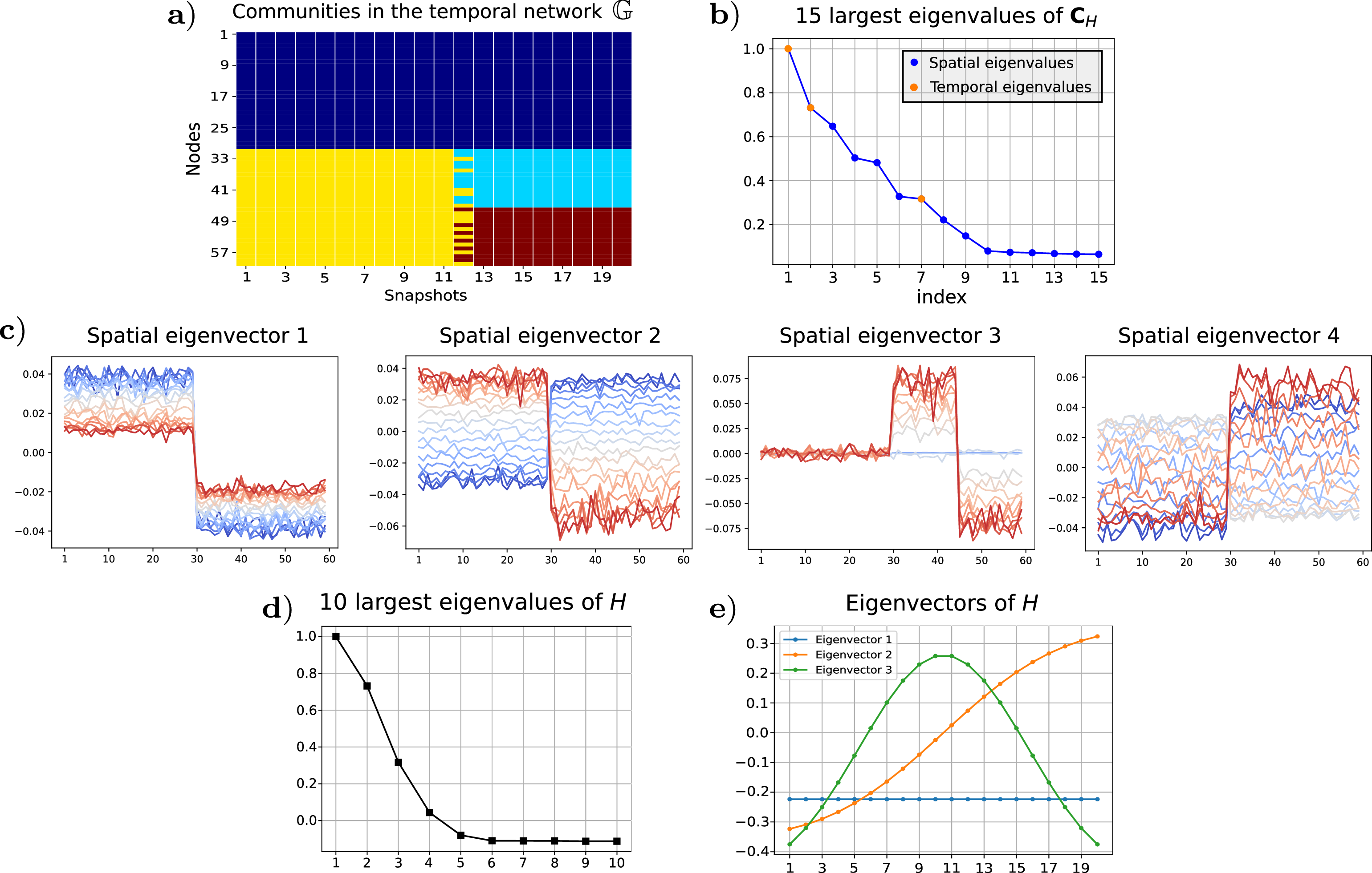
In figure 5 we illustrate the spectral clustering of the space–time network from example 1. The leading eigenvalues of \(\mathbf{C}_H\) are shown in figure 5b, with the spatial eigenvalues highlighted. The first four spatial eigenvectors of \(\mathbf{C}_H\) are displayed in figure 5c. For visualization purposes, each eigenvector \(\mathbf{f}^{\mathrm{spat},k}\) is folded into its \(M\) snapshot segments, which are displayed using a color gradient ranging from dark blue (\(\mathbf{f}_1^{\mathrm{spat},k}\)) to dark red (\(\mathbf{f}_M^{\mathrm{spat},k}\)). The sign structure of the first spatial eigenvector clearly separates nodes \(1\)–\(30\) from nodes \(31\)–\(60\), which shows that they are members of different communities throughout the entire network evolution. Additionally, the third spatial eigenvector distinguishes between nodes \(31\)–\(45\) and \(46\)–\(60\) during the second half of the evolution, indicating a split of the community around \(t=10\). Applying \(k\)-means to these two feature vectors we successfully recover all communities in the temporal network \(\mathbb{G}\) (figure 5a). This example also illustrates how slowly decaying modes of the coupling matrix \(H\) may interfere with the spatial eigenvectors (see remark 3). In particular, spatial eigenvectors 1, 2, and 4 in figure 5c can all be interpreted approximately as modulated versions of an observable separating the first 30 and last 30 nodes, where the modulation is induced by the first (blue), second (orange), and third (green) eigenvectors of \(H\), respectively (figure 5e), which correspond to three largest eigenvalues of \(H\) (figure 5d). This phenomenon complicates the direct application of standard spectral clustering methods, in which \(k\)-means is typically applied to the spatial eigenvectors corresponding to the dominant eigenvalues of \(\mathbf{C}_H\) preceding the spectral gap.
3.4 Computational complexity↩︎
The construction introduced above leads to a spatio-temporal transition matrix \(\mathbf{C}_H \in \mathbb{R}^{MN \times MN}\), where \(N\) denotes the number of nodes and \(M\) the number of snapshots. Consequently, the dimension of the associated eigenvalue problem scales with the product \(MN\) and can become prohibitively large for long temporal sequences or large networks.
The computational cost depends on the chosen snapshot coupling scheme and on the sparsity of the underlying network snapshots. In the most general setting, the matrix \(\mathbf{C}_H\) consists of \(M^2\) blocks of size \(N\times N\), yielding a storage complexity of order \(O(M^2N^2)\). Although practical implementations can exploit sparsity and the block structure of \(\mathbf{C}_H\), the computation of dominant eigenpairs remains the main computational bottleneck.
These observations motivate the development of a reduced-order representation of the spatio-temporal random walk. In the next section, we derive a projection-based reduction that preserves the essential spectral properties of \(\mathbf{C}_H\) while significantly reducing the computational effort required for community detection. More details on the computational complexity of our algorithm and its reduced version are given in appendix 9.
4 Model reduction↩︎
In this section, we develop a reduced model by restricting the search space for observables associated with each snapshot to suitably chosen low-dimensional subspaces. Since the snapshot observables that solve our objective 6 are expected to be approximately constant on communities, this reduction substantially lowers the memory requirements of the full model while preserving the essential community-level information (see remark 7).
4.1 Galerkin projection of covariance operators↩︎
Let \(\mathcal{W}_t = \mathrm{span}\{ w_1^t,\dots,w_{d_t}^t \} \subset \mathbb{U}\) be a \(d_t\)-dimensional subspace of observables associated with snapshot \(G_t\), equipped with the \(\boldsymbol{\mu}_t\)-weighted inner product. Let \(W_t = [\mathbf{w}_1^t,\dots,\mathbf{w}_{d_t}^t] \in \mathbb{R}^{N\times d_t}\) denote the matrix whose columns are the vector representations of the basis functions spanning \(\mathcal{W}_t\). We aim to solve 6 under the constraint that each observable \(f_t\) lies in \(\mathcal{W}_t\). Let \(\mathbf{a}_t \in \mathbb{R}^{d_t}\) denote the coordinate vector of \(\mathbf{f}_t\) with respect to the basis given by the columns of \(W_t\), so that \(\mathbf{f}_t = W_t \mathbf{a}_t\). The covariance of \(f_t\) can then be computed as \[\operatorname{var}(f_t) = \langle f_t,\, \mathcal{C}_{tt} f_t \rangle = \langle W_t \mathbf{a}_t,\, C_{tt}(W_t \mathbf{a}_t) \rangle = \langle \mathbf{a}_t,\, W_t^\top C_{tt} W_t \,\mathbf{a}_t \rangle.\] Similarly, we obtain the cross-covariance of observables \(f_t\in\mathcal{W}_t\) and \(f_{s}\in\mathcal{W}_{s}\) for \(t<s\) as \[\operatorname{cov}(f_t,f_s)=\langle f_t,\mathcal{C}_{ts}f_{s}\rangle=\langle W_t\mathbf{a}_t,C_{ts}(W_{s}\mathbf{a}_{s})\rangle=\langle\mathbf{a}_t,W_t^\top C_{ts}W_{s}\mathbf{a}_{s}\rangle.\] We define \[\widehat{C}_{tt}=W_t^\top C_{tt} W_t=W_t^{\top}D_{\mu_t}W_t\] and \[\widehat{C}_{ts}=W_t^\top\, C_{ts}\, W_{s}=W_t^{\top}D_{\mu_t}S_{ts}W_s.\] Now, analogously as in section 3.1 we derive the generalized eigenvalue problem that solves 7 restricted to subspaces of observables \(\mathcal{W}_t\), i.e., \[\label{eq:generalized95eval95problem95projected} \widehat{\mathbf{A}}_H\mathbf{a}=\widehat{\lambda}\widehat{\mathbf{B}}\mathbf{a},\tag{16}\] where \[\widehat{\boldsymbol{A}}_H= \begin{bmatrix} 0 & h_{12}\widehat{C}_{12} & \cdots & h_{1M}\widehat{C}_{1M} \\ h_{21} \widehat{C}_{12}^{\top} & 0 & \ddots & \vdots \\ \vdots & \ddots & \ddots & h_{(M-1)M}\widehat{C}_{(M-1)M} \\ h_{M1}\widehat{C}_{1M}^{\top} & \cdots & h_{M(M-1)}\widehat{C}_{(M-1)M}^{\top} & 0 \end{bmatrix},\widehat{\mathbf{B}}= \begin{bmatrix} \widehat{C}_{11} & 0 & \cdots & 0 \\ 0 & \widehat{C}_{22} & \ddots & \vdots \\ \vdots & \ddots & \ddots & 0 \\ 0 & \cdots & 0 & \widehat{C}_{MM} \end{bmatrix},\] \(\mathbf{a}=[\mathbf{a}_1^{\top},\mathbf{a}_2^{\top},...,\mathbf{a}_M^{\top}]^{\top}\) and \(\mathbf{a}_t\) is a coefficient vector containing coordinates of \(f_t\in\mathcal{W}_t\) with respect to the basis \(\{w_i^t\}_{i=1}^{d_t}\). Since all matrices \(W_t\) have full column rank, the matrices \(\widehat{C}_{tt}\) are invertible, and therefore so is \(\widehat{\mathbf{B}}\). Defining \[\label{eq:C95H95projected} \widehat{\mathbf{C}}_H=\widehat{\mathbf{B}}^{-1}\widehat{\mathbf{A}}_H,\tag{17}\] we can equivalently rewrite 16 as a standard eigenvalue problem \[\label{eq:eigenvalue95problem95reduced} \widehat{\mathbf{C}}_H\mathbf{a}=\widehat{\lambda}\mathbf{a}.\tag{18}\]
Solutions of 18 therefore give, for each snapshot \(t\), coefficient vectors \(\mathbf{a}_t\in\mathbb{R}^{d_t}\). To interpret them as snapshot observables, we lift each \(\mathbf{a}_t\) back to the full observable space \(\mathcal{W}_t\) by reconstructing \[\mathbf{f}_t = W_t \mathbf{a}_t, \qquad t=1,\ldots,M.\] The procedure is schematically illustrated in figure 6.
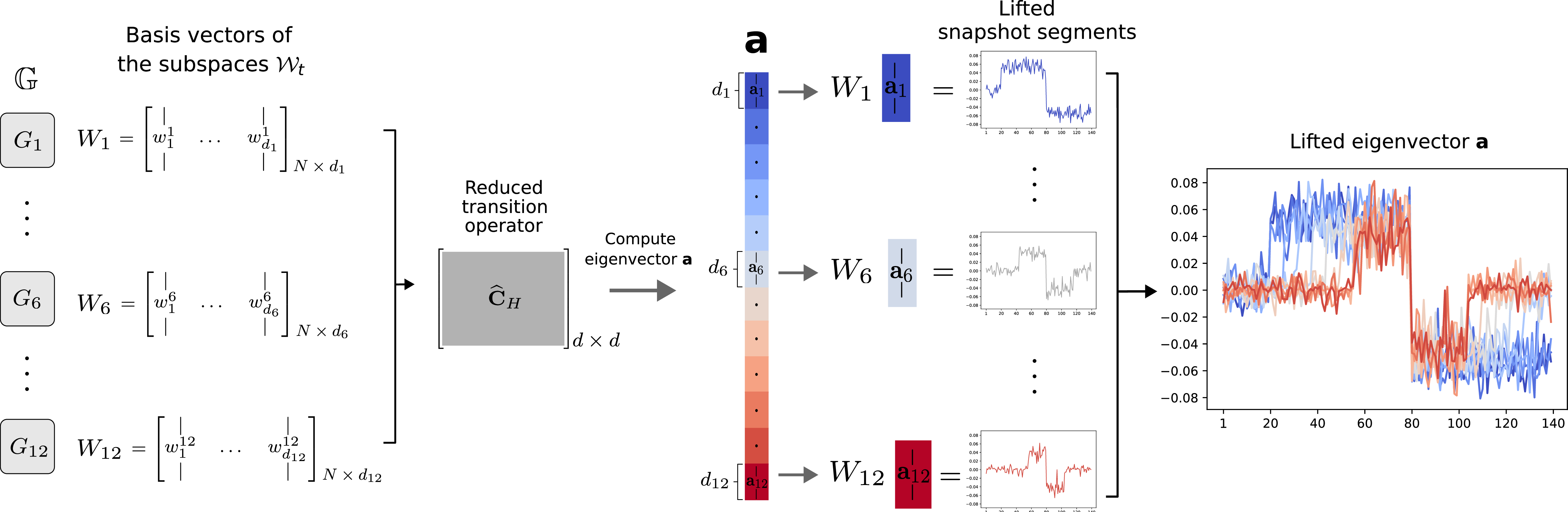
If the subspaces \(\mathcal{W}_t\) are chosen so that they contain observables whose level sets reflect the community structure in each snapshot, then the resulting space–time observables \(\mathbf{f}= [\mathbf{f}_1^{\top},\dots,\mathbf{f}_M^{\top}]^{\top}\) admit a clear interpretation in terms of how these communities evolve over time, as in the full (unprojected) model. A natural choice is, for example, to take \(\mathcal{W}_t\) as the subspace spanned by the dominant eigenvectors of the transition matrix of a random walk on the static network \(G_t\) (see example 5.2). In this case, eigenvectors \(\mathbf{a}\) of the reduced operator \(\widehat{\mathbf{C}}_H\) define, through lifting, space–time modes \(\mathbf{f}\) with \(\mathbf{f}_t\in \mathcal{W}_t\) that remain informative of the network community structure and can be directly compared to those of the full operator \(\mathbf{C}_H\), while being significantly cheaper to compute.
For \(1\le t<s\le M\), the building blocks of \(\widehat{\mathbf{C}}_H\) are given by \[[\widehat{\mathbf{C}}_H]_{ts}=h_{ts}\widehat{C}_{tt}^{-1}\widehat{C}_{ts}, \quad [\widehat{\mathbf{C}}_H]_{tt}=0, \quad [\widehat{\mathbf{C}}_H]_{st}=h_{st}\widehat{C}_{ss}^{-1}\widehat{C}_{ts}^{\top}\] where \[\label{eq:Kts95projection} \widehat{C}_{tt}^{-1}\widehat{C}_{ts}=(W_t^{\top}D_{\mu_t}W_t)^{-1}W_t^{\top}D_{\mu_t}K_{ts}W_{s}=\widehat{K}_{ts},\tag{19}\] and \[\label{eq:Tts95projection} \widehat{C}_{ss}^{-1}\widehat{C}_{ts}^{\top}=(W_{s}^{\top}D_{\mu_{s}}W_{s})^{-1}W_{s}^{\top}D_{\mu_{s}}T_{ts}W_t=\widehat{T}_{ts}.\tag{20}\] Let \[\mathcal{W}= \operatorname{colspan}(\mathbf{W})\] be the space spanned by the columns of the block diagonal matrix \(\mathbf{W}=\operatorname{diag}(W_1,\dots W_M)\in\mathbb{R}^{MN\times d}\) for \(d=\sum_{t=1}^Md_t\). More precisely, for each space–time obesrvable \(\mathbf{f}\) where \(\mathbf{f}_t=W_t\mathbf{a}_t\) we can write \[\mathbf{f}=\mathbf{W}\mathbf{a}.\] Then, we obtain \[\label{eq:C95H95Galerkin} \widehat{\mathbf{C}}_H=(\mathbf{W}^{\top}D_{\nu}\mathbf{W})^{-1}\mathbf{W}^{\top} D_{\nu}\mathbf{C}_H\mathbf{W}.\tag{21}\]
The building blocks \(\widehat{K}_{ts}\in\mathbb{R}^{d_t\times d_s}\) and \(\widehat{T}_{ts}\in\mathbb{R}^{d_s\times d_t}\) of matrix \(\widehat{\mathbf{C}}_H\) given in 19 and 20 are exactly Petrov–Galerkin projections of the transfer operators \(K_{ts}\) and \(T_{ts}\), where trial and test spaces may differ across snapshots. The reduced operator \(\widehat{\mathbf{C}}_H\in\mathbb{R}^{d\times d}\) 21 can be understood as a Galerkin projection of the full spatio-temporal operator \(\mathbf{C}_H\) onto \(\mathcal{W}\) with respect to the \(\boldsymbol{\nu}\)-weighted inner product.
Remark 4. Since \(\mathbf{C}_H\) acts as a transfer operator on the space–time network, this result is closely related to generalizations of Markov state models, which are obtained as Galerkin projections of transfer operators associated with dynamical processes onto suitably chosen low-dimensional subspaces [2]. This shows that our reduced model can be interpreted as a coarse-grained version of the spatio–temporal random walk that preserves the dominant spectral properties and long-time dynamics of the original process.
The operator \(\widehat{\mathbf{C}}_H\) inherits self-adjointness of \(\mathbf{C}_H\) as shown in the following lemma. Proofs of all lemmas stated in this section are provided in appendix 7.
Lemma 5. Let \(\mathbf{G}_{\mathcal{W}} = \mathbf{W}^{\top} D_{\nu}\mathbf{W}\) denote the Gram matrix induced by the \(\boldsymbol{\nu}\)-weighted inner product on the subspace \(\mathcal{W}\). Then the projected operator \(\widehat{\mathbf{C}}_H\) is self-adjoint with respect to the \(\mathbf{G}_{\mathcal{W}}\)-weighted inner product, i.e., \[\langle \widehat{\mathbf{C}}_H\mathbf{a},\mathbf{b}\rangle_{\mathbf{G}_{\mathcal{W}}} = \langle \mathbf{a},\widehat{\mathbf{C}}_H\mathbf{b}\rangle_{\mathbf{G}_{\mathcal{W}}}\] for all \(\mathbf{a},\mathbf{b}\in\mathbb{R}^{d}\), where \(\langle\mathbf{a},\mathbf{b}\rangle_{\mathbf{G}_{\mathcal{W}}}=\mathbf{a}^{\top}\mathbf{G}_{\mathcal{W}}\mathbf{b}\).
Remark 5. Defining \(\{w_1^t,\ldots,w_{d_t}^t\}\) to be the standard basis \(\{e_1,\ldots,e_N\}\) of \(\mathbb{R}^N\) for all \(1\leq t\leq M\) recovers the full formulation of our approach, since each observable space \(\mathcal{W}_t\) coincides with the full space \(\mathbb{U}\).
Spectral features of \(\mathbf{C}_H\) associated with slowly decaying space–time observables are well approximated by the spectrum of \(\widehat{\mathbf{C}}_H\), provided that the subspaces \(\mathcal{W}_t\) are appropriately chosen. We will later show that, under mild assumptions on the subspaces \(\mathcal{W}_t\), this connection can be made more precise. We begin with a general result about the spectrum of the projected operator \(\widehat{\mathbf{C}}_H\).
Lemma 6. Reduced operator \(\widehat{\mathbf{C}}_H\) defined in 21 has a real spectrum. For arbitrary subspaces \(\mathcal{W}_t\), its spectral radius satisfies \[\rho(\widehat{\mathbf{C}}_H) \leq 1.\]
Since \(\mathbf{W}\) is a block-diagonal matrix, the \(\boldsymbol{\nu}\)-orthogonal projector \(\mathbf{\Pi}_{\mathcal{W}}\) is given by \[\label{eq:Pi95W95diag} \mathbf{\Pi}_{\mathcal{W}}=\mathbf{W}(\mathbf{W}^\top D_{\nu}\mathbf{W})^{-1}\mathbf{W}^\top D_{\nu}=\operatorname{diag}(\mathbf{\Pi}_{\mathcal{W}_1}^{\mu_1},\dots,\mathbf{\Pi}_{\mathcal{W}_M}^{\mu_M}),\tag{22}\] where \(\mathbf{\Pi}_{\mathcal{W}_t}^{\mu_t}\) denotes the \(\boldsymbol{\mu}_t\)-orthogonal projector onto \(\mathcal{W}_t\). We note that the operators \(\widehat{\mathbf{C}}_H\) and \(\mathbf{\Pi}_{\mathcal{W}}\mathbf{C}_H|_{\mathcal{W}}\) are equivalent in the sense that they represent the same transformation expressed in different bases: the basis given by the columns of \(\mathbf{W}\) and the standard basis \(\{e_n\}_{n=1}^N\), respectively.
Analogously to theorem 2, we use the projected averaging operator \(\widehat{\mathbf{\Pi}}_{\mathrm{avg}}\) to split the reduced operator \(\widehat{\mathbf{C}}_H\) into temporal and spatial components. Let us define \[\label{eq:Pavg95galerkin} \widehat{\mathbf{\Pi}}_{\mathrm{avg}} = (\mathbf{W}^\top D_{\nu}\mathbf{W})^{-1}\mathbf{W}^\top D_{\nu}\,\mathbf{\Pi}_{\mathrm{avg}}\,\mathbf{W}.\tag{23}\] Using 13 we compute \(\widehat{\mathbf{\Pi}}_{\mathrm{avg}}\) as block diagonal-matrix with digaonal blocks given as \[(\widehat{\mathbf{\Pi}}_{\mathrm{avg}})_{tt}=(W_t^{\top}D_{\mu_t}W_t)^{-1}W_t^{\top}\mu_t(W_t^{\top}\mu_t)^{\top} \quad \text{ for } 1\le t\le M.\]
In the remainder of the paper, we will additionally impose the mild assumption that \(\mathbf{1}\in \mathcal{W}_t\) for all \(1 \le t \le M\), unless stated otherwise. In the following theorem we show that \(\widehat{\mathbf{C}}_H\) retains the fundamental spectral properties of \(\mathbf{C}_H\) and, analogously to the full operator, admits a decomposition into temporal and spatial components. Moreover, in theorem 8 we derive an error bound for the leading eigenvalues. This establishes the projected formulation as a computationally efficient but nevertheless accurate surrogate of the full operator.
Theorem 6. Let \(\widehat{\mathbf{C}}_H\) be a Galerkin projection of the spatio-temporal transition operator defined in 17 onto a subspace spanned by the columns of \(\mathbf{W}=\operatorname{diag}(W_1,\dots W_M)\). We assume that \(\mathbf{1}\in\operatorname{colspan}(W_t)\) for every \(1\le t\le M\). Then the operator \(\widehat{\mathbf{C}}_H\) admits the decomposition \[\widehat{\mathbf{C}}_H=\widehat{\mathbf{C}}_H^{\mathrm{temp}}+\widehat{\mathbf{C}}_H^{\mathrm{spat}},\] where \(\widehat{\mathbf{C}}_H^{\mathrm{temp}}\) and \(\widehat{\mathbf{C}}_H^{\mathrm{spat}}\) denote the compressions of \(\mathbf{C}_H^{\mathrm{temp}}\) and \(\mathbf{C}_H^{\mathrm{spat}}\) to the subspace \(\mathcal{W}\), that is, their projections restricted to \(\mathcal{W}\) and represented in the basis given by the columns of \(\mathbf{W}\). Moreover, it holds \[\widehat{\mathbf{C}}_H^{\mathrm{temp}}=\widehat{\mathbf{\Pi}}_{\mathrm{avg}}\,\widehat{\mathbf{C}}_H\,\widehat{\mathbf{\Pi}}_{\mathrm{avg}}, \quad \widehat{\mathbf{C}}_H^{\mathrm{spat}}=\widehat{\mathbf{\Pi}}_{\mathrm{avg}}^{\perp}\,\widehat{\mathbf{C}}_H\,\widehat{\mathbf{\Pi}}_{\mathrm{avg}}^{\perp}.\] Furthermore, the spectral radius of the projected transition operator is \(\rho(\widehat{\mathbf{C}}_H)=1\). The eigenpairs of \(\widehat{\mathbf{C}}_H\) coincide with the eigenpairs of \(\widehat{\mathbf{C}}_H^{\mathrm{temp}}\) and \(\widehat{\mathbf{C}}_H^{\mathrm{spat}}\) thereby partitioning the spectrum of \(\widehat{\mathbf{C}}_H\) into two classes:
The \(M\) eigenpairs of \(\widehat{\mathbf{C}}_H\) are obtained from the eigenpairs of \(\widehat{\mathbf{C}}_H^{\mathrm{temp}}\). The corresponding eigenvalues coincide with the temporal eigenvalues of \(\mathbf{C}_H\) (and therefore with the eigenvalues of the coupling matrix \(H\)) and are independent of the internal structure of the network snapshots. The corresponding eigenvectors are coefficient vectors in the column space basis \(\mathbf{W}\) of the temporal eigenvectors of \(\mathbf{C}_H\).
The remaining \(d - M\) eigenpairs of \(\widehat{\mathbf{C}}_H\) are obtained from the eigenpairs of \(\widehat{\mathbf{C}}_H^{\mathrm{spat}}\). The eigenpairs of \(\widehat{\mathbf{C}}_H\) from this class provide approximations of the leading spatial eigenpairs of the original operator \(\mathbf{C}_H\).
Proof. First, we recall that the averaging operator \(\mathbf{\Pi}_{\mathrm{avg}}\) is the orthogonal projection onto the subspace \[\operatorname{Im}(\mathbf{\Pi}_{\mathrm{avg}})=\operatorname{span}\{\,e_t\otimes\mathbf{1}\mid 1\le t\le M\,\}.\] Since \(\mathbf{1}\in\mathcal{W}_t\) for every snapshot, we have \(\operatorname{Im}(\mathbf{\Pi}_{\mathrm{avg}}) \subseteq\mathcal{W}\), and therefore \[\label{eq:PwPavg} \mathbf{\Pi}_{\mathcal{W}}\mathbf{\Pi}_{\mathrm{avg}}\mathbf{\Pi}_{\mathcal{W}}= \mathbf{\Pi}_{\mathrm{avg}}\mathbf{\Pi}_{\mathcal{W}} = \mathbf{\Pi}_{\mathcal{W}}\mathbf{\Pi}_{\mathrm{avg}} = \mathbf{\Pi}_{\mathrm{avg}}.\tag{24}\] Then, using the decomposition from theorem 2, we get \[\mathbf{\Pi}_{\mathcal{W}}\mathbf{C}_H|_{\mathcal{W}}=\mathbf{\Pi}_{\mathcal{W}}(\mathbf{C}_H^{\mathrm{temp}} + \mathbf{C}_H^{\mathrm{spat}})|_{\mathcal{W}}=\mathbf{\Pi}_{\mathcal{W}}\mathbf{C}_H^{\mathrm{temp}}|_{\mathcal{W}} + \mathbf{\Pi}_{\mathcal{W}}\mathbf{C}_H^{\mathrm{spat}}|_{\mathcal{W}},\] that is, \[\widehat{\mathbf{C}}_H=\widehat{\mathbf{C}}_H^{\mathrm{temp}}+\widehat{\mathbf{C}}_H^{\mathrm{spat}}.\] Substituting 21 and 23 into \(\widehat{\mathbf{\Pi}}_{\mathrm{avg}}\,\widehat{\mathbf{C}}_H\,\widehat{\mathbf{\Pi}}_{\mathrm{avg}}\) and \(\widehat{\mathbf{\Pi}}_{\mathrm{avg}}^{\perp}\,\widehat{\mathbf{C}}_H\,\widehat{\mathbf{\Pi}}_{\mathrm{avg}}^{\perp}\) and using 24 , we compute \[\widehat{\mathbf{\Pi}}_{\mathrm{avg}}\,\widehat{\mathbf{C}}_H\,\widehat{\mathbf{\Pi}}_{\mathrm{avg}}=\widehat{\mathbf{C}}_H^{\mathrm{temp}} \quad \text{and} \quad \widehat{\mathbf{\Pi}}_{\mathrm{avg}}^{\perp}\,\widehat{\mathbf{C}}_H\,\widehat{\mathbf{\Pi}}_{\mathrm{avg}}^{\perp}=\widehat{\mathbf{C}}_H^{\mathrm{spat}},\] which proves the claim. Furthermore, we have \[\mathbf{\Pi}_{\mathcal{W}}\mathbf{C}_H^{\mathrm{temp}}|_{\mathcal{W}}= \mathbf{\Pi}_{\mathcal{W}}\mathbf{\Pi}_{\mathrm{avg}}\mathbf{C}_H\mathbf{\Pi}_{\mathrm{avg}}|_{\mathcal{W}}=\mathbf{\Pi}_{\mathrm{avg}}\mathbf{C}_H\mathbf{\Pi}_{\mathrm{avg}}|_{\mathcal{W}}=\mathbf{C}_H^{\mathrm{temp}}|_{\mathcal{W}}\] so the nonzero eigenvalues of \(\mathbf{C}_H^{\mathrm{temp}}\) and \(\widehat{\mathbf{C}}_H^{\mathrm{temp}}\) coincide, and therefore \(1\in\sigma(\widehat{\mathbf{C}}_H^{\mathrm{temp}})\subset\sigma(\widehat{\mathbf{C}}_H)\). Using lemma 6, we conclude that \(\rho(\widehat{\mathbf{C}}_H)=1\). ◻
Remark 7 (Computational complexity). Assuming that the temporal network is sparse and that snapshots separated by at most \(r\) time steps are coupled, the construction of the full operator \(\mathbf{C}_H\) has computational complexity and memory requirements of order \(\mathcal{O}(MrN^2)\). In contrast, the reduced operator \(\widehat{\mathbf{C}}_H\) can be constructed in \(\mathcal{O}(MrNd_{\max}^2)\) time and requires \(\mathcal{O}(MrNd_{\max})\) memory, where \[d_{\max}=\max\{d_t\mid1\le t\le M\}.\] Typically, \(d_{\max}\ll N\), and the reduced formulation scales linearly with the number of nodes \(N\) so it provides substantial computational savings. Details of these estimates are given in appendix 9.
4.2 Error bound↩︎
Using the results from [34], [35], we can give error bounds on how accurately the projected operator \(\widehat{\mathbf{C}}_H\) approximates the spatial eigenvalues of \(\mathbf{C}_H\).
Theorem 8 (Error bound via projection onto reduced subspaces). Let \(1 \le m \le d\), and let \[\lambda_1^{\mathrm{spat}} \ge \cdots \ge \lambda_m^{\mathrm{spat}}\] be the leading spatial eigenvalues of the spatio-temporal transition matrix \(\mathbf{C}_H\), with corresponding \(\boldsymbol{\nu}\)-orthonormal eigenvectors \[\mathbf{f}^{\mathrm{spat},1}, \dots, \mathbf{f}^{\mathrm{spat},m}.\] Let \(\mathcal{W}_t\) be projection subspaces such that \(\mathbf{1}\in\mathcal{W}_t\) for all \(1\le t\le M\). Let \(\widehat{\lambda}_m^{\mathrm{spat}}\) be \(m\)th spatial eigenvalue of the reduced operator \(\widehat{\mathbf{C}}_H\) defined in 21 . The eigenvalue error \[E_m = \bigl|\lambda_m^{\mathrm{spat}} - \widehat{\lambda}_m^{\mathrm{spat}}\bigr|\] satisfies \[E_m \;\le\; (\lambda_1^{\mathrm{spat}} + 1) \sum_{i=1}^m \| \mathbf{\Pi}_{\mathcal{W}}^\perp \mathbf{f}^{\mathrm{spat},i} \|_\nu^2,\] and equivalently, \[\label{eq:extended95error} E_m \;\le\; (\lambda_1^{\mathrm{spat}} + 1) \sum_{i=1}^m \sum_{t=1}^M \pi_t\, \| (\mathbf{\Pi}_{\mathcal{W}_t}^{\mu_t})^\perp \mathbf{f}_t^{\mathrm{spat},i} \|_{\mu_t}^2.\qquad{(4)}\]
Proof. Since \(\mathbf{\Pi}_{\mathrm{avg}}^{\perp}\) is a projection, the operator \[\mathbf{C}_H^{\mathrm{spat}} = \mathbf{\Pi}_{\mathrm{avg}}^{\perp}\mathbf{C}_H\mathbf{\Pi}_{\mathrm{avg}}^{\perp}\] is self-adjoint with respect to the \(\boldsymbol{\nu}\)-weighted inner product. Let \(\mathcal{F} = \mathrm{span}(\mathbf{f}^{\mathrm{spat},1},\dots,\mathbf{f}^{\mathrm{spat},m})\). As \(\mathcal{F}\) is invariant under \(\mathbf{C}_H^{\mathrm{spat}}\), we may apply theorem 2.4 from [34]. Let \(\theta_1 \ge \dots \ge \theta_m\) be the principal angles between \(\mathcal{F}\) and \(\mathcal{W}\). Let \(\lambda_{\min(\mathcal{F}+\mathcal{W})}\) denote the smallest eigenvalue of the projection of \(\mathbf{C}_H^{\mathrm{spat}}\) onto the space \(\mathcal{F}+\mathcal{W}\). Then \[\label{eq:knyazev95clean} \begin{align} |\lambda_m^{\mathrm{spat}} - \widehat{\lambda}_m^{\mathrm{spat}}| &\le \sum_{i=1}^m |\lambda_i^{\mathrm{spat}} - \widehat{\lambda}_i^{\mathrm{spat}}| \\ &\le \sum_{i=1}^m (\lambda_i^{\mathrm{spat}} - \lambda_{\min(\mathcal{F}+\mathcal{W})}) \sin^2 \theta_i \\ &\le (\lambda_1^{\mathrm{spat}} - \lambda_{\min(\mathcal{F}+\mathcal{W})}) \sum_{i=1}^m \sin^2 \theta_i. \end{align}\tag{25}\] It remains to express \(\sum_{i=1}^m \sin^2 \theta_i\) in a convenient form. Let \(\mathbf{\Pi}= F F^\top D_\nu\) denote the \(\boldsymbol{\nu}\)-orthogonal projection onto \(\mathcal{F}\), where \(F = [\mathbf{f}^{\mathrm{spat},1},\dots,\mathbf{f}^{\mathrm{spat},m}]\in\mathbb{R}^{MN\times m}\). Let \(\sigma_i(A)\), \(\Lambda_i(A)\), and \(A^*\) denote the \(i\)th singular value, the \(i\)th eigenvalue, and the Hermitian transpose of an operator \(A\), respectively. Then the principal angles between the subspaces \(\mathcal{F}\) and \(\mathcal{W}\) are determined by the \(m\) largest singular values of \(\mathbf{\Pi}\mathbf{\Pi}_{\mathcal{W}}\) \[\cos^2(\theta_{m+1-i}) = \sigma_i^2(\mathbf{\Pi}\mathbf{\Pi}_{\mathcal{W}}) = \Lambda_i(\mathbf{\Pi}\mathbf{\Pi}_{\mathcal{W}}(\mathbf{\Pi}\mathbf{\Pi}_{\mathcal{W}})^*) = \Lambda_i(\mathbf{\Pi}\mathbf{\Pi}_{\mathcal{W}} \mathbf{\Pi}) \quad \text{ for }1\le i\le m.\] Hence, \[\sin^2(\theta_{m+1-i}) = 1-\Lambda_i(\mathbf{\Pi}\mathbf{\Pi}_{\mathcal{W}} \mathbf{\Pi})= \Lambda_i(\mathbf{\Pi}- \mathbf{\Pi}\mathbf{\Pi}_{\mathcal{W}} \mathbf{\Pi}) = \Lambda_i(\mathbf{\Pi}\mathbf{\Pi}_{\mathcal{W}}^{\perp} \mathbf{\Pi}) \quad \text{ for }1\le i\le m.\] Since \(\mathbf{\Pi}\mathbf{\Pi}_{\mathcal{W}}^{\perp} \mathbf{\Pi}\) has at most rank \(m\), we obtain \[\sum_{i=1}^m \sin^2(\theta_i) = \mathrm{tr}(\mathbf{\Pi}\mathbf{\Pi}_{\mathcal{W}}^{\perp} \mathbf{\Pi}).\] Substituting \(\mathbf{\Pi}= FF^\top D_\nu\) and using the identity \(\operatorname{tr}(AB)=\operatorname{tr}(BA)\) together with \(F^\top D_\nu F = I\), we obtain \[\operatorname{tr}(\mathbf{\Pi}\mathbf{\Pi}_{\mathcal{W}}^{\perp} \mathbf{\Pi}) = \operatorname{tr}(F^\top D_\nu \mathbf{\Pi}_{\mathcal{W}}^{\perp} F).\]
Using that \(\mathbf{\Pi}_{\mathcal{W}}^{\perp}\) is \(\boldsymbol{\nu}\)-self-adjoint, we obtain \[F^\top D_\nu \mathbf{\Pi}_{\mathcal{W}}^{\perp} F = (\mathbf{\Pi}_{\mathcal{W}}^{\perp} F)^\top D_\nu (\mathbf{\Pi}_{\mathcal{W}}^{\perp} F),\] and therefore \[\label{eq:energy95clean} \sum_{i=1}^m \sin^2(\theta_i) = \sum_{i=1}^m \|\mathbf{\Pi}_{\mathcal{W}}^{\perp} \mathbf{f}^{\mathrm{spat},i}\|_\nu^2.\tag{26}\] Since all eigenvalues of \(\mathbf{C}_H^{\mathrm{spat}}\) are contained in the interval \([-1,1]\) (see lemma 3), we have \(\lambda_{\min(\mathcal{F}+\mathcal{W})} \ge -1\) as well. Combining this with 25 and 26 we conclude \[|\lambda_m^{\mathrm{spat}} - \widehat{\lambda}_m^{\mathrm{spat}}| \le (\lambda_1^{\mathrm{spat}} + 1) \sum_{i=1}^m \|\mathbf{\Pi}_{\mathcal{W}}^{\perp} \mathbf{f}^{\mathrm{spat},i}\|_\nu^2.\]
Finally, inserting the block structure of \(\boldsymbol{\nu}\) and using 22 yields ?? . ◻
5 Numerical examples↩︎
In this section, we illustrate different aspects of our framework with the aid of three numerical examples. The first example demonstrates how the choice of snapshot coupling influences the detection of evolving and recurring communities. The second example compares the full and reduced formulations of the method and highlights the effectiveness of the proposed model reduction strategy. Finally, the third example applies our method to a temporal network generated from an opinion dynamics model. This example is based on an interacting-agent dynamical system designed to capture real-world collective behavior and demonstrates the ability of our approach to identify and track evolving communities in complex dynamical systems. In all examples, we use the heuristics described in appendix 10 to select the spatial eigenvectors used as feature coordinates for clustering.
5.1 Example 1 – recurrent communities↩︎
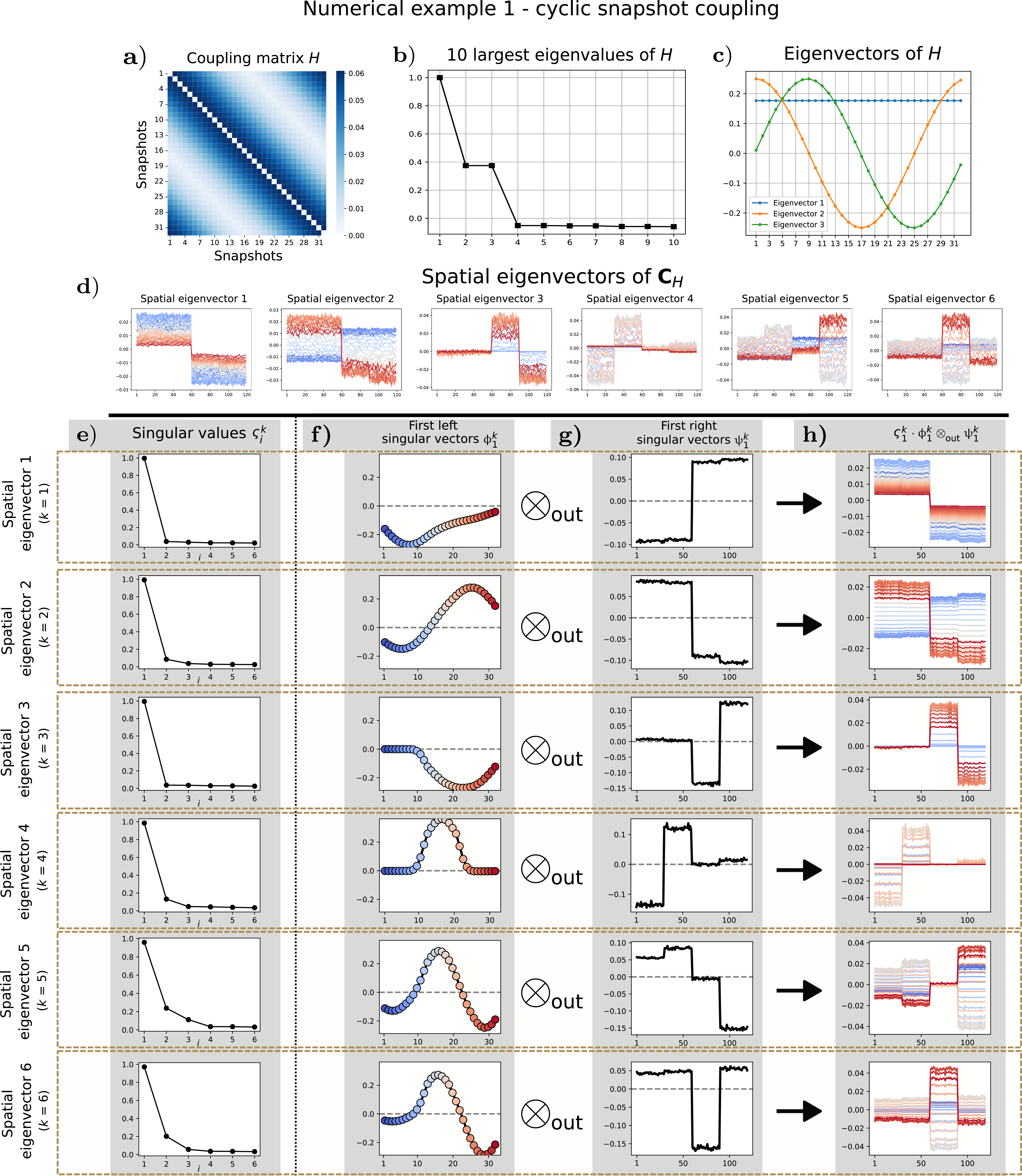
In this example we consider a temporal network \(\mathbb{G} = (G_1,\dots, G_{32})\) with 120 nodes consisting of 32 snapshots generated independently using a stochastic block model with intra-community probability \(p = 0.7\) and inter-community probability \(q = 0.05\). In snapshots \(G_1\)–\(G_8\), the network exhibits two stable communities \(C_1 = \{v_1,\dots,v_{60}\}\), \(C_2 = \{v_{61},\dots, v_{120}\}\). At snapshot \(G_9\), both communities \(C_1\) and \(C_2\) start gradually splitting into two smaller communities of equal size, \(C_{11} = \{v_1,\dots, v_{30}\}\), \(C_{12} = \{v_{31},\dots, v_{60}\}\), and \(C_{21} = \{v_{61},\dots, v_{90}\}\), \(C_{22} = \{v_{91},\dots, v_{120}\}\), respectively. This splitting process is completed by snapshot \(G_{12}\) and the resulting four-community structure then persists over snapshots \(G_{13}\)–\(G_{20}\). Lastly, communities \(C_{11}\) and \(C_{12}\) gradually merge again during the period \(G_{21}\)–\(G_{24}\) and after snapshot \(G_{25}\) the network has three stable communities \(C_1\), \(C_{21}\), and \(C_{22}\), which persist until the end of the evolution. We refer to these three stable regimes of the network evolution as phases 1, 2, and 3. The adjacency matrices of this temporal network are shown in figure 7a.
In this example, we employ the snapshot coupling scheme defined in ?? . Since the stable periods and structural changes occur on a longer time scale than in example 1, we choose a smaller decay parameter \(\alpha = 0.01\) in order to strengthen the coupling between snapshots over longer temporal distances. We consider two coupling matrices \(H_1\) and \(H_2\): a cyclic one (figure 7b), where the last snapshots are coupled to the first ones (in this case we set \(w_{ts}=\exp(-\alpha\min\{|t-s|,M-|t-s|\}^2)\) for \(1\le t,s\le M\)), and a non-cyclic one (figure 7c), where no such coupling is imposed.
By introducing cyclic coupling, our approach is able to correctly identify the reappearance of community \(C_1\) from phase 1 in phase 3 (figure 7g). In particular, the first spatial eigenvector in the cyclic coupling case separates the space–time nodes across all three phases into two large groups (figure 7e), while spatial eigenvectors 3 and 4 provide additional information about the splitting of communities \(C_1\) and \(C_2\) and the merging of communities \(C_{11}\) amd \(C_{12}\). This allows our approach to recover community \(C_1\) in phase 3. In contrast, without cyclic coupling, this would not be possible (figures 7h,i). The space–time observables describing the separation of community \(C_1\) from the rest of the network in phases 1 and 3 appear as two different spatial eigenvectors (eigenvectors 1 and 2 in figure 7f), due to the weak coupling between snapshots from these phases, while eigenvectors 3 and 6 describe the rest of structural changes. Although nodes \(v_1,\dots,v_{60}\) form a community in both phases, there is no information contained within leading eigenvectors of \(\mathbf{C}_H\) in this case indicating that these two communities are the same. Depending on whether we want to identify a densely connected group of nodes as the same community, even though it might have undergone structural changes between two periods of stability, we can, depending on the nature of the data, employ cyclic (or more generally long-range) couplings to detect such patterns.
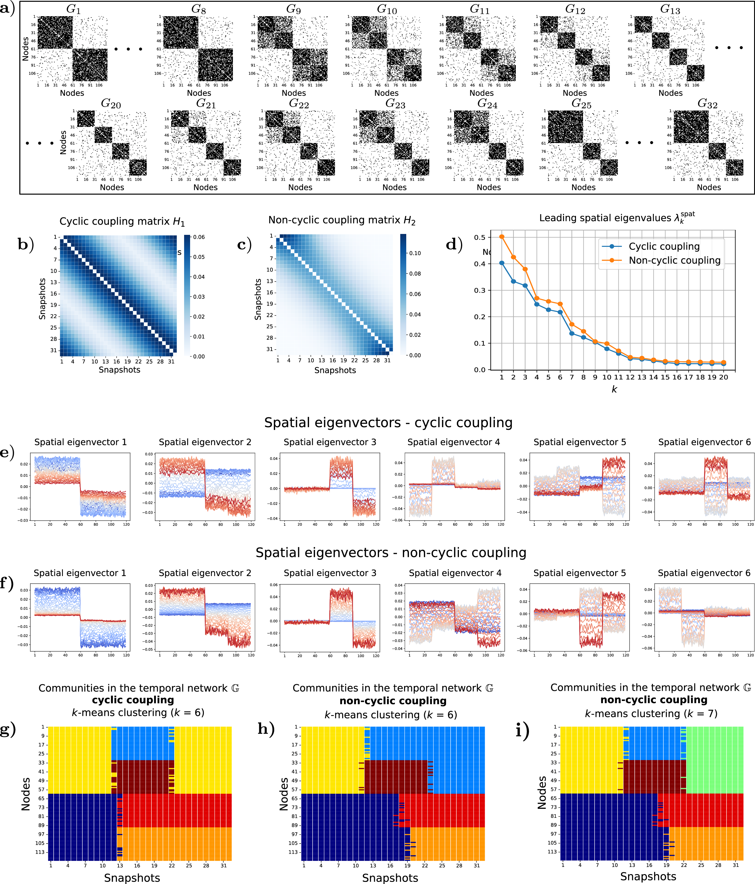
5.2 Example 2 – model reduction↩︎
In this example we perform a comparative analysis of the full and reduced approaches on a temporal network with 140 nodes. We choose again the coupling scheme defined in ?? with \(\alpha=0.03\) (figure 8b). Since the community structure of each snapshot is encoded in the dominant eigenvectors of the transition matrix \(S_t\) of a random walk defined on it, we use them to define the search spaces \(\mathcal{W}_t\). To further reduce computational requirements, instead of computing the full eigendecomposition of \(S_t\), we use an approximation of the dominant eigenvectors. In this example, we employ the Nyström method [36] to obtain good approximations by computing the eigendecomposition of a submatrix defined by a chosen node sample and extending the resulting eigenvectors to the full dimension. As shown in [36], relatively small node samples are often sufficient to obtain good approximations. In this experiment, we use samples obtained by selecting half of the nodes of the temporal network uniformly at random.
We therefore define the spaces \(\mathcal{W}_t\) to be spanned by the constant vector \(\mathbf{1}\in \mathbb{R}^N\) together with the approximated dominant eigenvectors of \(S_t\). In figure 8e, we compare the spatial eigenvalues of \(\mathbf{C}_H\) in the full model (blue) with those obtained from projections onto the subspaces \(\mathcal{W}_t\) (green). For comparison, we also include the spatial eigenvalues obtained when \(\mathcal{W}_t\) are spanned by the exact dominant eigenvectors of \(S_t\) (orange). In both cases, the spatial eigenvalues of the reduced models are close to those of the full model. In figure 8c, we show the leading spatial eigenvectors of \(\mathbf{C}_H\) and in figure 8d the network observables obtained by lifting eigenvectors of \(\widehat{\mathbf{C}}_H\). We observe that these network observables closely resemble the spatial eigenvectors of \(\mathbf{C}_H\), while being computed at a significantly lower computational cost.
Guided by the heuristics described in section 5.1, we select spatial eigenvectors 1 and 2 as feature vectors for the space–time node clustering. In figures 8f,h, we show the corresponding two-dimensional embeddings of space–time nodes, where each node is colored according to the snapshot it belongs to. Applying the \(k\)-means algorithm with \(k=3\), we see in figures 8g,i that the community structure of the temporal network is correctly identified in both cases, which demonstrates the effectiveness of the proposed reduced model.
Lastly, to further demonstrate the robustness of our method, we compare our snapshot coupling scheme with the method proposed in [22] which can be understood as a special case of our approach, where only the average correlation between successive snapshots is maximized (see the coupling matrix \(H_s\) in figure 8j). Since this coupling strategy only incorporates very local temporal interactions, it fails to adequately capture long-range temporal persistence of communities across snapshots. As a result, important temporal information is lost in the eigenvectors of \(\mathbf{C}_{H_s}\). In figure 8j, we show that the \(k\)-means clustering of the space–time nodes with feature coordinates given by the leading spatial eigenvectors of \(\mathbf{C}_{H_s}\) fails to correctly identify the evolving community structure of the temporal network.
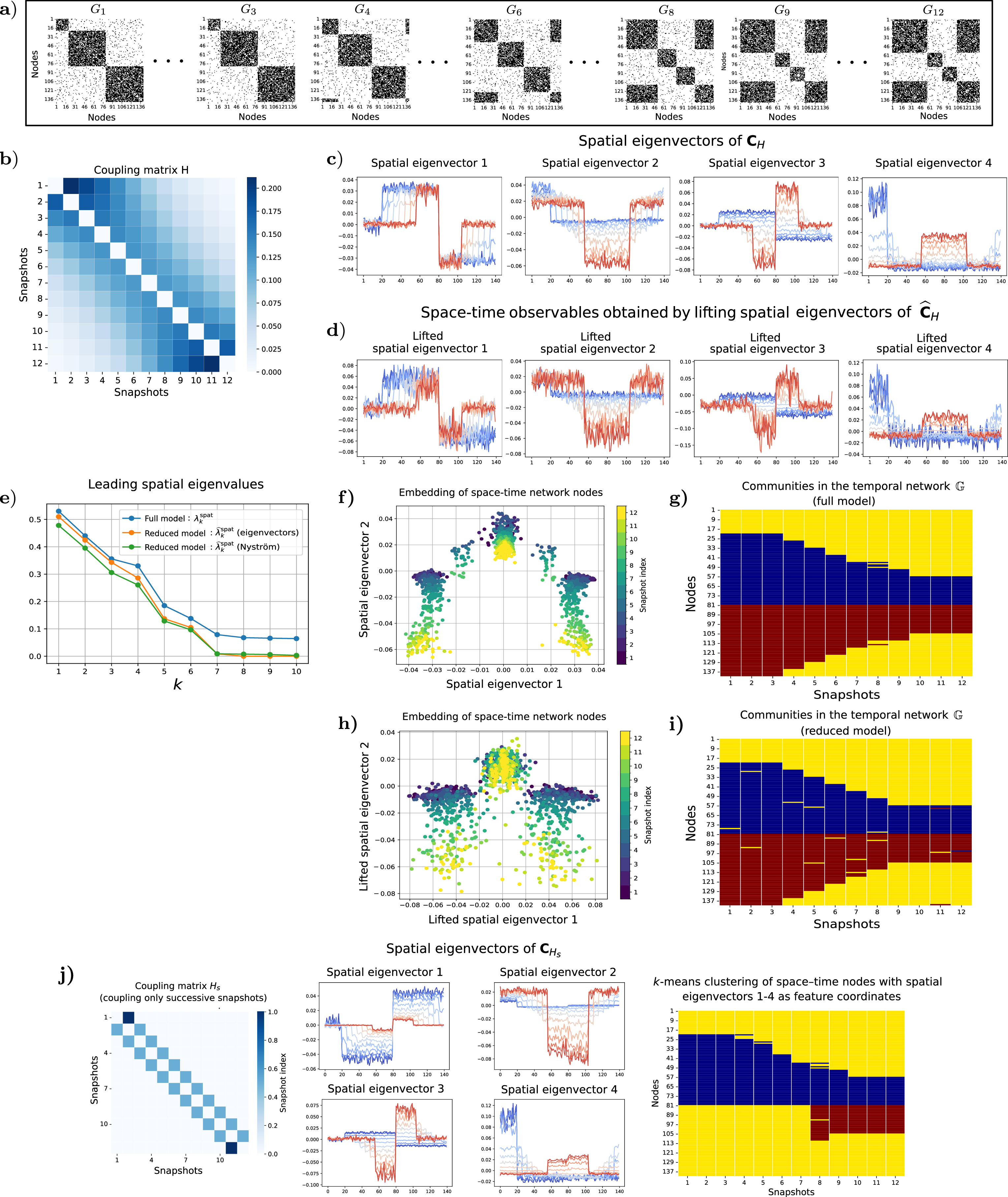
5.3 Example 3 – opinion dynamics↩︎
As a final example, we illustrate the applicability of our framework to clustering phenomena arising in interacting-agent systems, complementing transfer-operator based model reduction approaches [37]. We consider a modified version of the one-dimensional agent-based Hegselmann–Krause opinion dynamics model introduced in [38], which extends the classical Hegselmann–Krause model [39] by incorporating interactions between voters and political parties. We generate \(N=500\) agents, where the opinion of the \(i\)th agent at time \(t\) is denoted by \(x_i(t)\in[0,1]\). In addition to the voters, we assume there exist \(N_p=3\) political parties represented by highly influential agents with positions \(y_\alpha\) for \(\alpha\in\{1,2,3\}\) in the opinion space.
In this setting, voters form their opinions both through interactions with other voters and through interactions with political parties. As in the classical model, voters tend to align with nearby opinions in the opinion space, but they are also attracted toward parties whose political stance is close to their own. Simultaneously, political parties adapt their positions in response to the surrounding voter opinions in order to attract support, while also maintaining sufficient separation from competing parties in order to preserve their political identity. The resulting coupled voter–party dynamics are given by \[\label{eq:hegselmann95krause} \begin{align} \mathrm{d}x_i&=\gamma_{xx}F_{xx}(x_i)\mathrm{d}t+\gamma_{yx}F_{yx}(x_i)\mathrm{d}t+\sigma_x \mathrm{d}W_t^i,\\ \mathrm{d}y_{\alpha}&=\gamma_{xy}F_{xy}(y_{\alpha})\mathrm{d}t-\gamma_{yy}F_{yy}(y_{\alpha})\mathrm{d}t+\sigma_y \mathrm{d}W_t^{\alpha}. \end{align}\tag{27}\] Here, \(W^i, i=1,\dots,N\), and \(W^\alpha, \alpha=1,\dots,N_p\), are independent Brownian motions representing random external influences on voters and parties. The coefficients \(\sigma_x\) and \(\sigma_y\) determine the strength of the stochastic noise in the dynamics. The interaction forces are defined by \[\begin{align} F_{xx}(x_i)&=\frac{1}{N}\sum_{j=1}^{N}\mathbb{1}_{R_{xx}}(x_j-x_i)(x_j-x_i),\\ F_{yx}(x_i)&=\frac{1}{N_p}\sum_{\beta=1}^{N_p}\mathbb{1}_{R_{yx}}(y_{\beta}-x_i)(y_{\beta}-x_i),\\ F_{xy}(y_{\alpha})&=\frac{1}{N}\sum_{j=1}^{N}\mathbb{1}_{R_{xy}}(x_j-y_{\alpha})(x_j-y_{\alpha}),\\ F_{yy}(y_{\alpha})&=\frac{1}{N_p}\sum_{\beta=1}^{N_p}\mathbb{1}_{R_{yy}}(y_{\beta}-y_{\alpha})(y_{\beta}-y_{\alpha}), \end{align}\] where \(\mathbb{1}_R(x)\), \(R>0\) denotes the interaction kernel \[\mathbb{1}_R(x)= \begin{cases} 1, & |x|\le R, \\ 0, & |x|> R. \end{cases}\] The parameters \(R_{xx},R_{yx},R_{xy}\), and \(R_{yy}\) denote the interaction radii governing voter–voter, voter–party, party–voter, and party–party interactions, respectively. The constants \(\gamma_{xx},\gamma_{xy},\gamma_{yx},\gamma_{yy}\ge0\) determine the strength of the contribution of the corresponding interaction forces to the overall dynamics. A detailed discussion of these parameters and their sociopolitical interpretation can be found in [38].
We simulate the system 27 with parameters \(R_{xx}=0.04, R_{yx}=0.1,R_{xy}=0.5, R_{yy}=0.05\) and \(\gamma_{xx}=0.5,\gamma_{yx}=0.9,\gamma_{xy}=0.01,\gamma_{yy}=0.015\) for 390 time steps using time step size 0.05. The noise coefficients are set to \(\sigma_x=0.025, \sigma_y=0.002\). Initially, voters’ opinions are sampled uniformly from the interval \([0,1]\), while the initial party positions are given by \(y_1(0)=0.15, y_2(0)=0.35\) and \(y_3(0)=0.9\). The trajectories of voters in the opinion space are shown by blue lines in figure 9a, while the trajectories of the three political parties are shown in red.
Under this parameter regime (see section 4 in [38]), the system eventually reaches consensus, with both voters and parties converging toward a common opinion. However, the evolution exhibits several clearly distinguishable phases. Initially, three separate opinion communities emerge around the three political parties. Since parties \(y_1\) and \(y_2\) begin with relatively similar political positions, the corresponding voter groups gradually approach one another and eventually merge as illustrated in figure 9a. In contrast, the community associated with party \(y_3\), which initially occupies the opposite side of the opinion spectrum, remains separated for a substantially longer period. Finally, the remaining two communities merge, leading to near-consensus across the population.
From this simulation, we construct a weighted temporal network on the set of voters consisting of 40 snapshots of the system taken at times \(t=0,10,20,\dots,390\), indicated by dashed lines in figure 9a. For each snapshot, edge weights between nodes are determined according to the distance between the corresponding opinions, so that voters with similar opinions are connected by edges of larger weight \[w(x_i,x_j)=e^{-\frac{(x_i-x_j)^2}{2\varepsilon^2}},\] where we set \(\varepsilon=0.05\). The resulting weighted adjacency matrices are then used as input for our framework.
We apply the reduced version of our algorithm with coupling parameter \(\alpha=0.01\) in the matrix \(H\). The subspaces \(\mathcal{W}_t\) are chosen to be spanned by the dominant eigenvectors of the transition matrices associated with random walks on the network snapshots. We cluster space–time nodes using spatial eigenvectors 1 and 3 shown in figure 9c as feature coordinates. The resulting communities are shown in figure 9b. During the initial phase, the algorithm identifies three distinct communities (light blue, orange, and red). Around \(t=15\), the orange and red communities merge into a larger dark blue community. Later, around \(t=25\), the remaining light blue community merges with the dark blue one. Since the dark blue community already contains a substantially larger number of nodes, the algorithm identifies this event not as a symmetric merge but rather as the absorption of the smaller light blue community into the dominant dark blue community, which then persists until the end of the simulation.
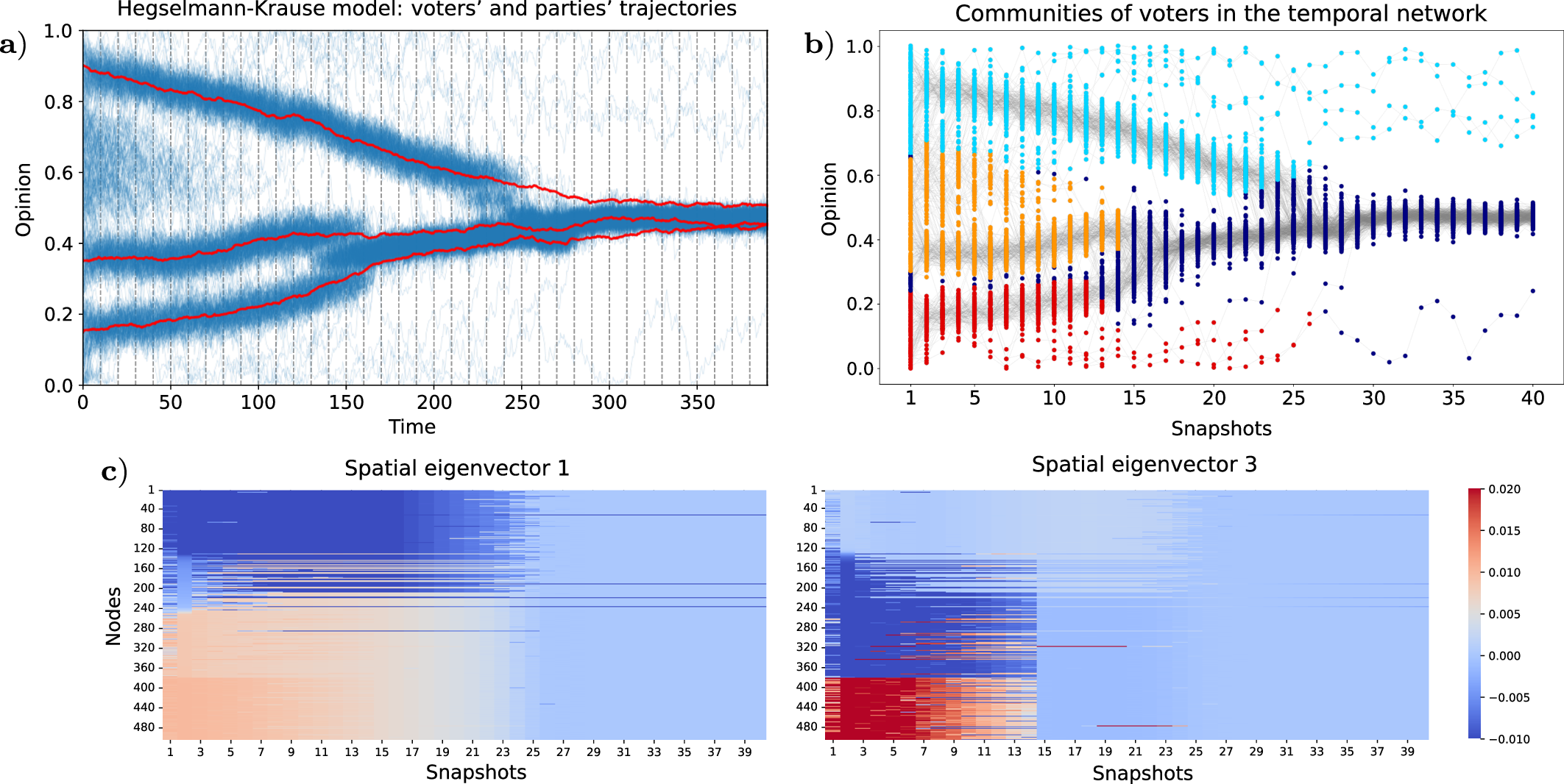
6 Conclusion↩︎
In this work, we developed a transfer operator-based framework for community detection in temporal networks. Building on multi-view canonical correlation analysis, we introduced a general snapshot coupling scheme that allows correlations between snapshots to be incorporated into a unified objective function. This flexibility enables the method to adapt to different application scenarios while reducing the influence of noisy fluctuations and spurious temporal effects.
A central contribution of this work is the interpretation of the resulting multi-view CCA formulation through the lens of a spatio-temporal random walk on an augmented static network. We showed that the optimization problem reduces to a generalized eigenvalue problem whose spectral properties can be analyzed using known techniques. This perspective provides a natural dynamical interpretation of temporal communities as metastable structures of the associated spatio-temporal process and establishes a direct connection between temporal community detection and well-understood concepts from the analysis of static networks.
Furthermore, we investigated how temporal effects induced by the snapshot coupling scheme interact with spatial effects arising from the network structure. In particular, we have shown that not all dominant eigenvectors necessarily contain meaningful information about community structure and proposed heuristics for identifying informative spatial modes. Both our theoretical and computational analysis contribute to a better understanding of the spectral signatures of evolving communities and highlights the importance of separating temporal artifacts from genuine structural changes.
To improve scalability, we derived a reduced-order formulation based on projections onto low-dimensional subspaces. We showed that the key spectral properties of the full model carry over to the reduced setting and established error bounds that quantify the approximation quality. Numerical experiments show that the reduced model is capable of recovering evolving community structures while significantly reducing computational costs.
Several interesting directions remain for future research. On the theoretical side, a deeper understanding of the spectral properties of the spatio-temporal operator and more principled criteria for selecting informative spatial eigenvectors would be desirable. It would also be interesting to investigate adaptive and data-driven choices of the snapshot coupling matrix, as well as connections to other formulations of temporal and multilayer networks. Finally, applying the proposed methodology to empirical temporal networks from social, biological, and technological domains may provide additional insights into the structure and dynamics of complex systems.
Funding↩︎
This work has been partially funded by the Deutsche Forschungsgemeinschaft (DFG, German Research Foundation) under Germany’s Excellence Strategy – The Berlin Mathematics Research Center MATH+ (EXC-2046/1, EXC-2046/2, project ID: 390685689) and by the Federal Ministry of Research, Technology and Space (BMFTR) project EPISERVE (funding ID: 031L0324A), member of the German Modeling network for severe infectious diseases, MONID)
Additional Information↩︎
The authors declare no competing interests.
7 Proofs of lemmas from sections 3.2 and 4.1↩︎
Proof of lemma 1. Define \(\boldsymbol{\pi}= [\pi_1, \dots, \pi_M]^\top \in \mathbb{R}^M\) by \[\pi_t = \frac{r_t}{R}>0, \qquad R = \sum_{t=1}^M r_t.\] Then \(\sum_{t=1}^M \pi_t = 1\), so \(\boldsymbol{\pi}\) is a probability distribution. Moreover, for all \(t,s\), we have \[\pi_t h_{ts} = \frac{r_t}{R} \cdot \frac{w_{ts}}{r_t} = \frac{r_s}{R} \cdot \frac{w_{st}}{r_s} = \pi_s h_{st},\] which proves the detailed balance condition. The weighted degree of node \(t\) in \(G_H\) is \[\deg_H(t) = \sum_{s=1}^M (W_H)_{ts} = r_t,\] so that the transition matrix of a random walk on \(G_H\) is indeed \[D_H^{-1} W_H = H,\] where \(D_H = \operatorname{diag}(\deg_H(1), \dots, \deg_H(M))\). This random walk is reversible by the detailed balance condition and the uniqueness of \(\boldsymbol{\pi}\) follows if \(G_H\) is connected. ◻
Proof of lemma 2. Since all \(S_t\) are row-stochastic, we have \(S_t\mathbf{1}=\mathbf{1}\) for all \(1\le t\le M\). Consequently, for \(t<s\), we obtain \(K_{ts}\mathbf{1}=(S_t\cdots S_{s-1})\mathbf{1}=\mathbf{1}\) and by the definition of probability distributions \(\mu_t\), it holds that \((K_{ts})^{\top}\boldsymbol{\mu}_t=\boldsymbol{\mu}_s\). Hence, \(T_{ts}\mathbf{1}=D_{\mu_s}^{-1}(K_{ts})^{\top}D_{\mu_t}\mathbf{1}=D_{\mu_s}^{-1}(K_{ts})^{\top}\boldsymbol{\mu}_t=D_{\mu_s}^{-1}\boldsymbol{\mu}_{s}=\mathbf{1}\). Finally, since the coupling matrix \(H\) is row-stochastic, we obtain for \(\mathbf{1}_{MN}\in\mathbb{R}^{MN}\) and \(\mathbf{1}_N\in\mathbb{R}^N\) that \(\mathbf{C}_H\mathbf{1}_{MN}=[(\sum_{s=1}^Mh_{1s})\mathbf{1}_N^{\top},\dots,(\sum_{s=1}^Mh_{Ms})\mathbf{1}_N^{\top}]^{\top}=\mathbf{1}_{MN}\). Therefore, \(\mathbf{C}_H\) is row-stochastic as well. The claim \(\rho(\mathbf{C}_H)=1\) then follows from standard properties of row-stochastic matrices and the largest eigenvalue is \(\lambda=1\). ◻
Lemma 7. Let \((X_\tau^{(\mathbf{C}_H)})_{\tau=1}^\infty\) denote the spatio-temporal random walk on \(V\times\{1,\dots,M\}\) given by the transition matrix \(\mathbf{C}_H\). Its dynamics in the temporal dimension is governed by the transition matrix \(H\). More precisely, let \[\bar{X}_{\tau}^{(\mathbf{C}_H)}=\operatorname{pr}_2(X_{\tau}^{(\mathbf{C}_H)})\] where \(\operatorname{pr}_2\) denotes the projection onto the second coordinate. Then, \((\bar{X}_{\tau}^{(\mathbf{C}_H)})_{\tau=1}^{\infty}\) is a well-defined random walk and \[p\Big(\bar{X}_{\tau+1}^{(\mathbf{C}_H)}=s|\bar{X}_{\tau}^{(\mathbf{C}_H)}=t\Big)=h_{ts}.\]
Proof. Let \[B_{ts}= \begin{cases} K_{ts}, & t<s,\\ 0, &t=s,\\ T_{st}, &t>s. \end{cases}\] Then \[p\Big(X_{\tau+1}^{(\mathbf{C}_H)}=(v_j,s)\mid X_{\tau}^{(\mathbf{C}_H)}=(v_i,t)\Big)=h_{ts}(B_{ts})_{ij}.\] Thus, the expression \[\sum_{j=1}^Np\Big(X_{\tau+1}^{(\mathbf{C}_H)}=(v_j,s)\mid X_{\tau}^{(\mathbf{C}_H)}=(v_i,t)\Big)=\sum_{j=1}^Nh_{ts}(B_{ts})_{ij}=h_{ts}\sum_{j=1}^N(B_{ts})_{ij}=h_{ts}\] is independent of \(i\), and therefore the following is well-defined \[\begin{align} h_{ts}&=\sum_{j=1}^Np\Big(X_{\tau+1}^{(\mathbf{C}_H)}=(v_j,s)\mid X_{\tau}^{(\mathbf{C}_H)}=(v_i,t)\Big)=\sum_{j=1}^Np\Big(X_{\tau+1}^{(\mathbf{C}_H)}=(v_j,s)\mid \bar{X}_{\tau}^{(\mathbf{C}_H)}=t\Big)\\&=p\Big(\bar{X}_{\tau+1}^{(\mathbf{C}_H)}=s|\bar{X}_{\tau}^{(\mathbf{C}_H)}=t\Big). \qedhere \end{align}\] ◻
Proof of lemma 3. Let \(\boldsymbol{\pi}=[\pi_1,\dots,\pi_M]^{\top}\in\mathbb{R}^M\) be defined as in lemma 1. Let \[\boldsymbol{\nu} = \big[\pi_1 \boldsymbol{\mu}_1^\top ,\, \pi_2 \boldsymbol{\mu}_2^\top ,\, \dots,\, \pi_M \boldsymbol{\mu}_M^\top \big]^\top \in \mathbb{R}^{MN}.\] In the proof we use the following identities: For \(t<s\), it holds that \[\boldsymbol{\mu}_{s}^\top T_{ts} = \boldsymbol{\mu}_sD_{\mu_s}^{-1}(K_{ts})^{\top}D_{\mu_t}=\mathbf{1}^{\top}(K_{ts})^{\top}D_{\mu_t}=\mathbf{1}^{\top} D_{\mu_t}=\boldsymbol{\mu}_t^\top\] and \[\boldsymbol{\mu}_t^\top K_{ts} = \boldsymbol{\mu}_t^{\top}(S_t\cdots S_{s-1})=\boldsymbol{\mu}_{t+1}^{\top}(S_{t+1}\dots S_{s-1})=\cdots=\boldsymbol{\mu}_{s-1}^{\top}S_{s-1}=\boldsymbol{\mu}_{s}^\top .\] Let \((\boldsymbol{\nu}^\top \mathbf{C}_H)_t \in \mathbb{R}^N\) and \(\boldsymbol{\nu}_t\) denote the \(t\)th segments (of length \(N\)) of the vectors \(\boldsymbol{\nu}^\top \mathbf{C}_H\) and \(\boldsymbol{\nu}\), respectively. For every \(1 \le t \le M\), we have \[\begin{align} (\boldsymbol{\nu}^\top \mathbf{C}_H)_t = \sum_{k=1}^{t-1} h_{kt}\,\pi_k\,\boldsymbol{\mu}_k^\top K_{kt} \;+\; \sum_{k=t+1}^{M} h_{kt}\,\pi_k\,\boldsymbol{\mu}_k^\top T_{tk} = \sum_{k=1}^{M} h_{kt}\,\pi_k \,\boldsymbol{\mu}_t^\top . \end{align}\] As shown in lemma 1, \(\pi_t h_{tk}=\pi_k h_{kt}\), which, with the row-stochasticity of \(H\), gives \[\Big( \sum_{k=1}^{M} \pi_k h_{kt} \Big)\boldsymbol{\mu}_t^\top = \Big( \sum_{k=1}^{M} h_{tk} \Big)\pi_t \boldsymbol{\mu}_t^\top = \pi_t \boldsymbol{\mu}_t^\top = \boldsymbol{\nu}_t^\top .\] Hence, \(\boldsymbol{\nu}^\top \mathbf{C}_H = \boldsymbol{\nu}^\top\), and \(\boldsymbol{\nu}\) is a stationary distribution of \(\mathbf{C}_H\). Since \(T_{ts}^{\top}D_{\mu_{s}}=D_{\mu_t}K_{ts}\) and \(D_{\mu_{s}}T_{ts}=K_{ts}^{\top}D_{\mu_t}\), the detailed balance condition \[D_{\nu}\mathbf{C}_H=\mathbf{C}_H^\top D_{\nu}\] holds so the random walk induced by \(\mathbf{C}_H\) is time-reversible with respect to \(\boldsymbol{\nu}\). Consequently, the matrix \(\mathbf{C}_H\) is then self-adjoint with respect to \(\boldsymbol{\nu}\)-weighted inner product. Therefore, its spectrum is real. Since its spectral radius additionally satisfies \(\rho(\mathbf{C}_H)=1\) (see lemma 2) all eigenvalues are contained in the interval \([-1,1]\). ◻
Proof of lemma 4. From 12 it is easy to see that \(\mathbf{\Pi}_{\mathrm{avg}}^2=\mathbf{\Pi}_{\mathrm{avg}}\). Furthermore, \(\mathbf{\Pi}_{\mathrm{avg}}\) is self-adjoint with respect to the \(\boldsymbol{\nu}\)-weighted inner product. Indeed, using 13 , for any two observables \(\mathbf{f}, \mathbf{g}\), we obtain \[\langle\mathbf{\Pi}_{\mathrm{avg}}\mathbf{f},\mathbf{g}\rangle_{\nu}= \sum_{t=1}^M\pi_t\langle\mathbf{1}\boldsymbol{\mu}_t^{\top}\mathbf{f}_t,\mathbf{g}_t\rangle_{\mu_t}=\sum_{t=1}^M\pi_t\langle\mathbf{1},\mathbf{f}_t\rangle_{\mu_t}\langle\mathbf{1},\mathbf{g}_t\rangle_{\mu_t}=\sum_{t=1}^M\pi_t\langle\mathbf{f}_t,\mathbf{1}\mu_t^{\top}\mathbf{g}_t\rangle_{\mu_t}=\langle\mathbf{f},\mathbf{\Pi}_{\mathrm{avg}}\mathbf{g}\rangle_{\nu}.\] Since \(\mathbf{\Pi}_{\mathrm{avg}}\) is idempotent and \(\boldsymbol{\nu}\)-self-adjoint, it is a \(\boldsymbol{\nu}\)-orthogonal projection. Finally, \[\operatorname{Im}(\mathbf{\Pi}_{\mathrm{avg}}) = \operatorname{span}\{e_t\otimes\mathbf{1}\mid 1\le t\le M\},\] follows directly from the definition of \(\mathbf{\Pi}_{\mathrm{avg}}\). ◻
Proof of lemma 5. We have \[\begin{align} \langle\widehat{\mathbf{C}}_H\mathbf{a},\mathbf{b}\rangle_{\mathbf{G}_{\mathcal{W}}}&=\mathbf{a}^{\top}\widehat{\mathbf{C}}_H^{\top}\mathbf{W}^{\top}D_{\nu}\mathbf{W}\mathbf{b}\\ &=\mathbf{a}^{\top}\mathbf{W}^{\top}\mathbf{C}_H^{\top}D_{\nu}\mathbf{W}(\mathbf{W}^{\top}D_{\nu}\mathbf{W})^{-{\top}}\mathbf{W}^{\top} D_{\nu}\mathbf{W}\mathbf{b}\\&=\mathbf{a}^{\top}\mathbf{W}^{\top} D_{\nu}\mathbf{C}_H\mathbf{W}\mathbf{b}\\ &=\mathbf{a}^{\top}\mathbf{W}^{\top} D_{\nu}\mathbf{W}(\mathbf{W}^{\top} D_{\nu}\mathbf{W})^{-1}\mathbf{W}^{\top} D_{\nu}\mathbf{C}_H\mathbf{W}\mathbf{b}\\ &=\langle\mathbf{a},\widehat{\mathbf{C}}_H\mathbf{b}\rangle_{\mathbf{G}_{\mathcal{W}}}, \end{align}\] where the third equality follows from the detailed balance condition of \(\mathbf{C}_H\) with respect to \(\nu\) (see lemma 3), and in the fourth equality we insert the identity \(I = \mathbf{W}^{\top} D_{\nu}\mathbf{W}\, (\mathbf{W}^{\top} D_{\nu}\mathbf{W})^{-1}\). ◻
Proof of lemma 6. Since \(\widehat{\mathbf{C}}_H\) is self-adjoint with respect to the \(\mathbf{G}_{\mathcal{W}}\)-weighted inner product, its spectrum is real-valued. For any \(\mathbf{a}\in\mathbb{R}^d\), we have \[\|\mathbf{W}\mathbf{a}\|_\nu^2 = \mathbf{a}^{\top} \mathbf{W}^{\top} D_\nu \mathbf{W}\mathbf{a}= \|\mathbf{a}\|_{\mathbf{G}_{\mathcal{W}}}^2 .\] Let \(\mathbf{\Pi}_{\mathcal{W}}\) denote the \(\boldsymbol{\nu}\)-orthogonal projector onto \(\mathcal{W}\). Using the definition of the Galerkin projection, \[\mathbf{W}\widehat{\mathbf{C}}_H \mathbf{a} = \mathbf{\Pi}_{\mathcal{W}}\mathbf{C}_H \mathbf{W}\mathbf{a}.\] Hence, \[\|\widehat{\mathbf{C}}_H \mathbf{a}\|_{\mathbf{G}_{\mathcal{W}}} = \|\mathbf{W}\widehat{\mathbf{C}}_H \mathbf{a}\|_\nu = \|\mathbf{\Pi}_{\mathcal{W}}\mathbf{C}_H \mathbf{W}\mathbf{a}\|_\nu \le \|\mathbf{C}_H \mathbf{W}\mathbf{a}\|_\nu \le \|\mathbf{C}_H\|_\nu\,\|\mathbf{W}\mathbf{a}\|_\nu,\] where the first inequality follows from the contractivity of the \(\boldsymbol{\nu}\)-orthogonal projector \(\mathbf{\Pi}_{\mathcal{W}}\). Since \(\|\mathbf{C}_H\|_\nu\le 1\), we conclude that \[\|\widehat{\mathbf{C}}_H \mathbf{a}\|_{\mathbf{G}_{\mathcal{W}}} \le \|\mathbf{W}\mathbf{a}\|_\nu = \|\mathbf{a}\|_{\mathbf{G}_{\mathcal{W}}}.\] Therefore, \[\|\widehat{\mathbf{C}}_H\|_{\mathbf{G}_{\mathcal{W}}} \le 1 .\] Finally, self-adjointness of \(\widehat{\mathbf{C}}_H\) with respect to the \(\mathbf{G}_{\mathcal{W}}\)-weighted inner product implies that its induced norm coincides with its spectral radius. Hence \[\rho(\widehat{\mathbf{C}}_H) = \|\widehat{\mathbf{C}}_H\|_{\mathbf{G}_{\mathcal{W}}} \le 1. \qedhere\] ◻
8 Formal description of a space–time network↩︎
We formalize the construction of the space–time network \(\mathscr G_H=(\mathscr V, \mathscr E, \omega)\) as follows. The bijection \[\zeta : V \times \{1,\dots, M\} \rightarrow \{1,\dots, MN\}, \qquad (v_i,t) \mapsto (t-1)N + i,\] flattens the space–time nodes and allows us to define a new state space \[\mathscr V = \zeta\big(V \times \{1,\dots,M\}\big) = \{1,\dots ,MN\}.\] Thus, we can interpret \(\mathbf{C}_H\) as the transition matrix of a random walk on a weighted undirected network \(\mathscr G_H\), where the edge weights are given by the function \(\omega\) as summarized in lemma 8.
Lemma 8. Let \(t<s\). Within the network \(\mathscr G_H=(\mathscr V, \mathscr E, \omega)\) associated to a temporal network \(\mathbb{G}\) with a coupling matrix \(H\), an edge \[e_{ij}^{ts} = \big(\zeta(v_i,t),\,\zeta(v_j,s)\big) \in \mathscr E\subset \mathscr V\times\mathscr V\] exists if and only if snapshots \(G_t\) and \(G_s\) are coupled with nonzero weight \(h_{ts}\) and a temporal path of length \(s-t\) exists from \(v_i \in G_t\) to \(v_j \in G_s\), that is, if and only if \[h_{ts}(K_{ts})_{ij} \neq 0.\] The weight of edge \(e_{ij}^{ts}\) is defined as \[\omega(e_{ij}^{ts}) = \nu(\zeta(v_i,t))(\mathbf{C}_H)_{\zeta(v_i,t),\,\zeta(v_j,s)}=\pi_t\mu_t(v_i)(\mathbf{C}_H)_{\zeta(v_i,t),\,\zeta(v_j,s)}.\] where \(\mu_t\) is defined in 3 , and \(\boldsymbol{\pi}\) and \(\boldsymbol{\nu}\) are as defined in lemmas 1 and 3, respectively. Then, the transition matrix of a random walk on \(\mathscr G\) is given by \(\mathbf{C}_H\).
Proof. First, let us show that the edge weight is well defined. Let \(t<s\). Then \[\omega(e_{ij}^{ts}) = \pi_t\mu_t(v_i)h_{ts}(K_{ts})_{ij} = \pi_sh_{st}\mu_t(v_i)(K_{ts})_{ij} = \pi_sh_{st}\mu_s(v_j)(T_{ts})^{\top}_{ij} = \pi_s\mu_s(v_j)h_{st}(T_{ts})_{ji} = \omega(e_{ji}^{st}),\] where the second equality follows from the detailed balance condition \(D_{\pi} H = H^{\top} D_{\pi}\), and the third equality follows from the relation \(D_{\mu_t} K_{ts} = T_{ts}^{\top} D_{\mu_s}\).
An edge \(e_{ij}^{ts}\) exists if and only if its weight is nonzero. Since \[\omega(e_{ij}^{ts}) = \pi_t \mu_t(v_i)\, (\mathbf{C}_H)_{\zeta(v_i,t),\,\zeta(v_j,s)},\] and \(\pi_t \mu_t(v_i) > 0\), we have \[\omega(e_{ij}^{ts}) \neq 0 \;\Longleftrightarrow\; (\mathbf{C}_H)_{e_{ij}^{ts}} \neq 0 \;\Longleftrightarrow\; h_{ts}(K_{ts})_{ij} \neq 0.\]
Lastly, for a vertex \(\zeta(v_i,t)\) in \(\mathscr V\) we have \[\deg(\zeta(v_i,t))=\sum_{s=1}^M\sum_{j=1}^N\omega(e_{ij}^{ts})=\sum_{s=1}^M\sum_{j=1}^N\pi_t\mu_t(v_i)(\mathbf{C}_H)_{\zeta(v_i,t),\,\zeta(v_j,s)}=\pi_t\mu_t(v_i)\sum_{s=1}^Mh_{ts}=\pi_t\mu_t(v_i).\] Let the degree matrix \(D_{\mathscr G_H} \in \mathbb{R}^{MN \times MN}\) be defined as \[D_{\mathscr G_H} = \operatorname{diag}(\deg(\zeta(v_1,1)),\dots,\deg(\zeta(v_N,M)))\] and let \(\mathscr W\in\mathbb{R}^{MN\times MN}\) be a weighted adjacency matrix such that \(\mathscr W_{\zeta(v_i,t),\,\zeta(v_j,s)}=\omega(e_{ij}^{ts})\). Then the transition matrix of the random walk on \(\mathscr G_H\) is \[D_{\mathscr G_H}^{-1} \mathscr W = \mathbf{C}_H. \qedhere\] ◻
In this way, by connecting nodes across different network snapshots, we obtain a multilayer static network representation of the temporal network \(\mathbb{G}\) that preserves both the temporal coupling of snapshots and their internal structural properties.
9 Computational complexity analysis↩︎
Here, we discuss and compare the computational complexity and memory requirements of the full and reduced formulations of our algorithm. Throughout this discussion, we assume that the temporal network is sparse, i.e., that the transition matrices \(S_t\) are sparse. This is a natural assumption in many real-world applications [40], [41].
9.0.0.1 Full model.
The main computational bottleneck in both the full and reduced models is the construction of the matrices \(\mathbf{C}_H\) and \(\widehat{\mathbf{C}}_H\), respectively. The computational complexity depends on the sparsity pattern of the snapshot coupling matrix \(H\). Suppose that snapshots separated by at most \(r\) time steps are coupled and define \[r=\max\{|t-s|:h_{ts}\neq0\}.\] Then \(H\) contains \(\mathcal{O}(Mr)\) nonzero entries. Consequently, for each \(1\le t\le M\), at most \(r\) block matrices \(K_{ts}\) must be computed. These building blocks of \(\mathbf{C}_H\) can be computed recursively via \(K_{t,s+1}=K_{ts}S_s\), so that already computed matrices can be reused. Hence, for each block row of \(\mathbf{C}_H\), at most \(r\) matrix multiplications are required. Although the matrices \(S_t\) are sparse, their products \(S_{ts}\) generally become dense for larger temporal distances. Therefore, each recursive multiplication has computational complexity \(\mathcal{O}(N^2)\), resulting in a total cost of \(\mathcal{O}(rN^2)\) per block row and \(\mathcal{O}(MrN^2)\) for computing all blocks \(K_{ts}\). Since the blocks \(T_{ts}\) are obtained from \(K_{ts}\) by transposition and diagonal rescaling, their computation has the same asymptotic complexity. Consequently, the total complexity of constructing \(\mathbf{C}_H\) scales quadratically with the number of nodes \(N\) as \(\mathcal{O}(MrN^2)\). The dominant eigenvectors of the sparse matrix \(\mathbf{C}_H\) can be computed efficiently using e.g. iterative eigensolvers such as the Lanczos algorithm [42] or the Nyström method [36]. Regarding memory requirements, the main bottleneck is storing the matrix \(\mathbf{C}_H\). Since \(\mathbf{C}_H\) contains \(\mathcal{O}(Mr)\) nonzero blocks of size \(N\times N\), the total memory requirements are \(\mathcal{O}(MrN^2)\).
9.0.0.2 Reduced model.
Let \[d_{\mathrm{max}}=\max\{d_t:1\le t\le M\}.\] Using similar arguments as above together with the recursive relation \(K_{ts}W_s=S_t(K_{t+1,s}W_s)\), the \(\mathcal{O}(Mr)\) projected covariance blocks \(\widehat{C}_{ts}\) can be computed in \(\mathcal{O}(MrNd_{\mathrm{max}}^2)\) time. Furthermore, computing the matrices \(\widehat{C}_{tt}^{-1}\) requires \(\mathcal{O}(MNd_{\mathrm{max}}^2+Md_{\mathrm{max}}^3)\) operations. Once these matrices are available, assembling all projected transfer operators \(\widehat{K}_{ts}\) and \(\widehat{T}_{ts}\) requires \(\mathcal{O}(Mrd_{\mathrm{max}}^3)\) operations. Since typically \(d_{\mathrm{max}}\ll N\), summing everything up we obtain the overall computational complexity for computing \(\widehat{\mathbf{C}}_H\) to be \(\mathcal{O}(MrNd_{\mathrm{max}}^2)\) which scales linearly with \(N\). Furthermore, the reduced formulation provides substantial memory savings. Indeed, storing the sparse matrices \(S_t, D_{\mu_t}\), the basis vectors that define the subspaces \(\mathcal{W}_t\), and the reduced operator \(\widehat{\mathbf{C}}_H\) in total require \(\mathcal{O}(MrNd_{\mathrm{max}})\) space which also scales only linearly with \(N\).
10 Heuristics for selecting spatial eigenvectors for clustering↩︎
Since the spatio-temporal random walk can be decomposed into temporal and spatial components (see lemma 7), the spectral properties of the transition matrix \(\mathbf{C}_H\) are influenced by both the spectral properties of the coupling matrix \(H\) and the multi-step transfer operators. In particular, slowly decaying non-constant eigenvectors of \(H\) that do not correspond to metastable behavior of the temporal component of the spatio-temporal random walk can still influence some of the leading spatial eigenvectors of \(\mathbf{C}_H\). As a consequence, not every leading spatial eigenvector can be interpreted as describing coherent sets of the spatio-temporal random walk.
Such effects can be recognized in spatial eigenvectors whose snapshot segments are approximately given by scalar multiples of a base observable carrying information about the spatial organization of nodes. In figure 10d we show the leading spatial eigenvectors of the example 1 (see section 5.1). The segments of the first and second spatial eigenvectors can both be interpreted approximately as scalar multiples of observables separating the first and last 60 nodes. While the first spatial eigenvector is informative, in the sense that it indicates that these two groups remain coherent and separated from each other throughout the whole evolution, this information is lost in the second spatial eigenvector. More precisely, the corresponding base observable is modulated in this case by a non-constant, slowly decaying eigenvector of the coupling matrix \(H\) shown in figure 10a. This eigenvector, plotted in green in figure 10c, corresponds to the third largest eigenvalue of \(H\) (figure 10b) and does not reflect metastability of the temporal component of the spatio-temporal random walk. Consequently, the second spatial eigenvector is not useful as a feature coordinate for clustering.
On the other hand, some informative spatial eigenvectors may correspond to relatively small eigenvalues of \(\mathbf{C}_H\). This occurs when they capture structural changes only during specific phases of the evolution, while carrying no spatial information during the remaining time intervals. For example, the fourth spatial eigenvector in figure 10d captures spatial organization of the nodes only during phase 2, which accounts for approximately one third of the total time. Due to this interplay between temporal and spatial effects, there is typically no clear spectral gap among the leading eigenvalues of \(\mathbf{C}_H\) (see figure 7d) as it is expected in community detection algorithms for static networks. Consequently, standard approaches based on selecting spatial eigenvectors corresponding to the slowest time scales before a spectral gap are not directly applicable. Although a definitive solution to this problem remains open and will be addressed in future work, we provide heuristic guidelines for the coupling schemes considered in this work.
To detect these spurious metastability effects among spatial eigenvectors, we consider the matrices \[F_k= \begin{bmatrix} (\mathbf{f}^{\mathrm{spat},k}_1)^\top\\ \vdots\\ (\mathbf{f}^{\mathrm{spat},k}_M)^\top \end{bmatrix} \in\mathbb{R}^{M\times N},\] whose rows are the snapshot segments of the spatial eigenvectors \(\mathbf{f}^{\mathrm{spat},k}\). We now look at its singular value decomposition \[F_k=\Phi_k\Sigma_k\Psi_k^{\top}= \sum_{i=1}^{\min(M,N)} \varsigma_i^k\cdot\phi_i^k\otimes_{\mathrm{out}}\psi_i^k,\] where the columns of \(\Phi_k=[\phi_1^k,\dots,\phi_M^k]\in\mathbb{R}^{M\times M}\) and \(\Psi_k=[\psi_1^k,\dots,\psi_N^k]\in\mathbb{R}^{N\times N}\) are the left and right singular vectors of \(F_k\), respectively, \(\Sigma_k\in\mathbb{R}^{M\times N}\) is the rectangular diagonal matrix containing the singular values \[\varsigma_1^k\geq \varsigma_2^k\geq \dots \geq \varsigma_{\min(M,N)}^k\] and \(\otimes_{\mathrm{out}}\) denotes the outer product of vectors.
Spatial eigenvectors can now be interpreted as modulations of observables given by the dominant right singular vectors \(\psi_1^k\) (figure 10g), while the type of the modulation by slowly decaying eigenvectors of \(H\) is reflected in the corresponding left singular vectors \(\phi_1^k\) (figure 10f).
In this example we consider the first six spatial eigenvectors. Since \[\varsigma_1^k \gg \varsigma_2^k \geq \dots \geq \varsigma_{32}^k,\] as shown in figure 10e, we consider the approximations \[F_k\approx \varsigma_1^k\cdot\phi_1^k\otimes_{\mathrm{out}}\psi_1^k,\] for \(1\leq k\leq 6\) (compare figure 10d and figure 10h). By inspecting the dominant left singular vectors (figure 10f), we observe that, as shown in figure 10h, the second spatial eigenvector is approximately obtained by modulating a base observable (figure 10g) with the third eigenvector of \(H\) (plotted in green in figure 10c), while the fifth and sixth spatial eigenvectors are approximately obtained by modulating base observables with the second eigenvector of \(H\) (plotted in orange in figure 10c). We therefore exclude these spatial eigenvectors from the feature coordinates used for clustering and apply a clustering algorithm to spatial eigenvectors 1, 3 and 4.
Furthermore, by examining the support of the dominant left singular vectors \(\phi_1^3\) and \(\phi_1^4\), we observe that the third spatial eigenvector carries structural information during the second and third phases of the evolution, whereas the fourth spatial eigenvector carries structural information only during the second phase.