Grounded Iterative Language Planning:
How Parameterized World Models Reduce Hallucination Propagation in LLM Agents
June 26, 2026
Abstract
World models for language agents come in two useful forms. An agent-based world model calls an LLM API and reasons flexibly in language, but its errors appear as hallucinated state changes that are hard to score with ordinary regression losses. A parameterized world model is a trained transition predictor; its errors are easier to measure with quantities such as NodeMSE, delta accuracy, and validity accuracy, but it is usually weaker as a standalone planner. We compare these two families on four graph-structured planning benchmarks and introduce operational hallucination metrics for the agent-based case. The comparison motivates Grounded Iterative Language Planning (GILP), which trains only a small parameterized backbone and combines it with API-based agent reasoning. The backbone supplies valid actions, predicted state deltas, risk, and value; the LLM drafts an action and imagined delta; and a consistency gate asks for revision when the two disagree. On real GPT-4o-mini calls, GILP reduces hallucinated-state rate from \(0.176\) to \(0.035\). In calibrated simulator ablations, it raises success from 0.668to 0.838while adding only \(\sim\)22%extra LLM calls. Code: https://github.com/Hik289/Environment-reduce-error.git.
1 Introduction↩︎
Large language models (LLMs) are now a common backbone for autonomous agents, whether they are called through OpenAI’s chat.completions [1], Anthropic’s messages [2], or the Google Gemini endpoint [3]. In chain-of-thought and ReAct-style planning [4]–[9], the agent is not only choosing
actions. It is also acting as an agent-based world model: it writes what it thinks the next state will be, then uses that text in the next decision. This is useful because goals, tool calls, and observations all live in the same medium, and the
recipe works well on many interactive benchmarks [10]–[14].
The hard part is that not all world-model errors look the same. A parameterized world model has an explicit prediction target, so its error can be computed directly: NodeMSE on node states, delta accuracy on changed nodes, validity accuracy on actions, and so on. An agent-based world model is different. Its transition is a piece of language and structured JSON produced by an API model. The most damaging errors are semantic hallucinations: a completion that did not happen, a dependency that is ignored, or an entity state that is written into the history and reused later. These errors are not well described by a single MSE. We therefore define operational metrics for them: hallucinated-state rate, propagation depth, and long-horizon error growth.
This leads to the central comparison of the paper. Parameterized world models have measurable and often lower transition error, but they are weak semantic planners. Agent-based world models reason well, but their hallucinations are harder to measure and compound over long horizons. In our experiments, the agent baseline’s per-step error probability climbs to 0.393by step ten, its hallucinated-state rate reaches 0.205, and a hallucinated atom persists for a mean of 2.45steps. The natural question is whether a small amount of trained parameterization can be used to control the hallucination error of an API-based agent without giving up its reasoning ability.
1.0.0.1 Motivating example.
Consider a six-step workflow with tasks \(\{1,\dots,6\}\). At step three the agent’s imagined transition declares “task 3: completed” although the environment kept it pending (the precondition was missed in the JSON
serialisation). The model continues to plan against the corrupted state, emits execute(task_5) which depends on task 3, the environment rejects it as invalid, and the agent patches with three more hallucinated state atoms before the episode
times out. One false token generated three invalid actions. We see this cascade both in the calibrated simulator and in direct GPT-4o-mini API calls. JSON-mode enforcement [1] helps with syntax; it does not by itself stop the agent from believing a false state.
1.0.0.2 Two world models.
We study both sides explicitly. The agent-based world model is the LLM planner: it calls an API, reasons over the serialized task, chooses an action, and writes an imagined next-state delta. The parameterized world model is a small trained network [15]–[18] that predicts action validity, next-state deltas, completion, value, and risk. The latter has ordinary supervised errors, including NodeMSE and delta accuracy; the former needs hallucination metrics because its mistakes live in generated state claims. The two models therefore fail in complementary ways.
1.0.0.3 Our approach: GILP.
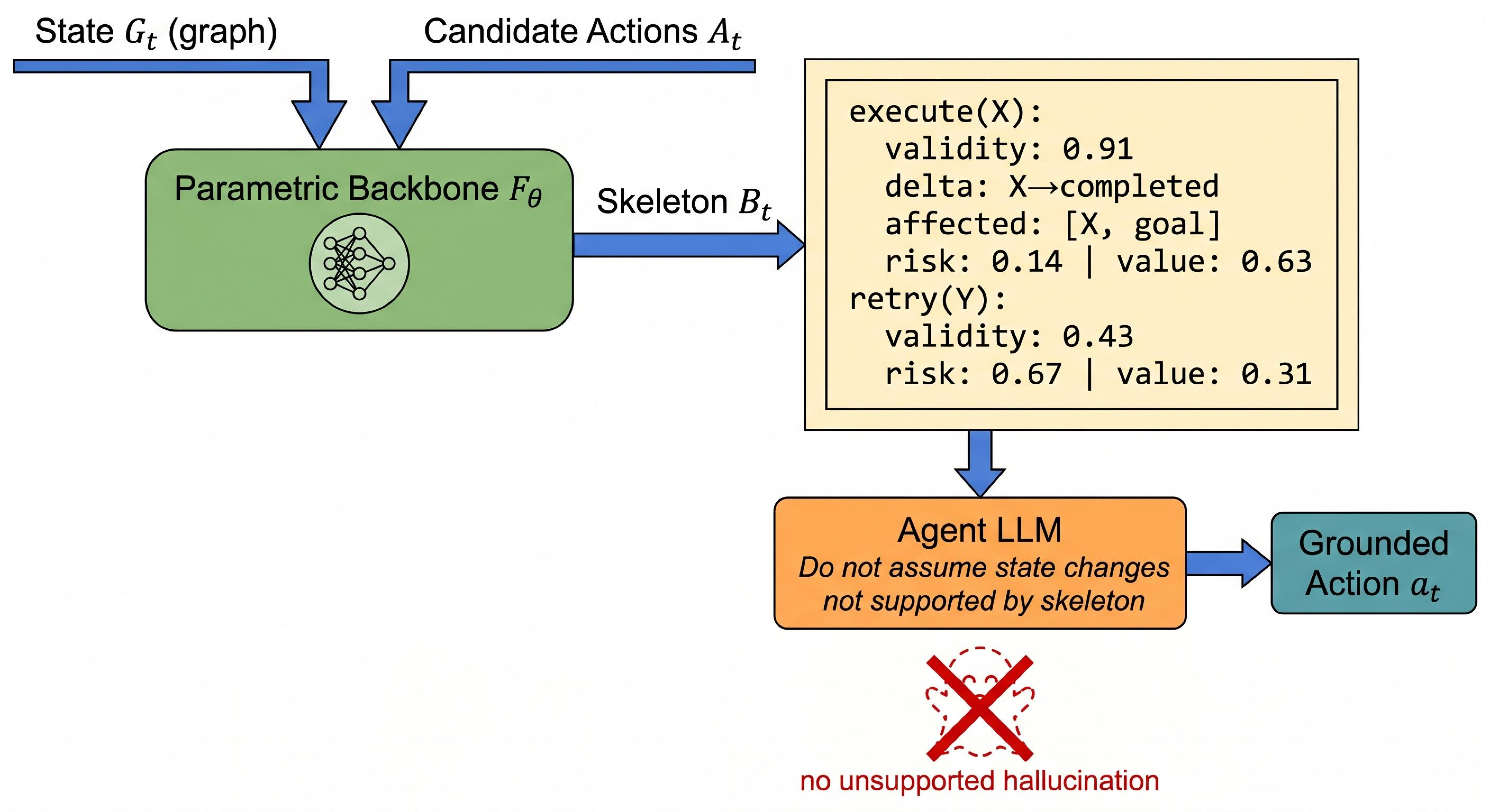
We propose Grounded Iterative Language Planning (GILP) to combine them. GILP trains only a small parameterized backbone, then keeps the API agent as the reasoning engine. At each step, the backbone scores candidate actions and serialises a compact skeleton: validity, predicted delta, risk, affected entities, and value. The LLM drafts an action and an imagined next-state delta in structured JSON. A Jaccard consistency gate compares the agent’s delta with the parameterized prediction; when consistency falls below \(\tau_{\text{low}}{=}0.30\), the agent receives a short correction message that names the disagreeing atoms. The goal is not to make the parameterized model solve the task. It is to use its measurable transition signal to reduce the hallucination error of the agent-based world model.
1.0.0.4 Contributions.
We frame long-horizon planning as a comparison between two world models: an agent-based model with flexible API reasoning and a parameterized model with measurable supervised transition error.
We define hallucination propagation as the agent-based analogue of world model error and measure it with HSR, PD, and long-horizon error-probability proxies.
We introduce GILP, which trains a small parameterized backbone and uses it to correct the hallucinated state deltas of an API-based reasoning agent.
We show that GILP improves both task success and state faithfulness: simulator success rises from 0.668to 0.838, real GPT-4o-mini HSR falls by \(80\%\), and long-horizon success improves from 0.471 to 0.758.
We release the prompt suite (Appendix 9), simulator, benchmarks, and code artifacts for reproducible follow-up work.
2 Related Work↩︎
2.0.0.1 LLMs as language world models.
A growing line of work treats LLM agents as implicit world models that generate next-state predictions in natural language as part of chain-of-thought planning. ReAct [5] interleaves reasoning and action so that each thought predicts a downstream outcome; Reflexion [7] adds verbal self-critique that updates the agent’s belief about past predictions; Plan-and-Solve [9] forces commitment to a complete imagined trajectory before execution; Tree of Thoughts and Graph of Thoughts [8], [19] branch the rollout into a search tree; LATS [20] unifies reasoning, acting, and planning via language agent tree search; RAP [6] uses the LLM as the transition model inside MCTS. The same paradigm drives benchmark and embodied deployments [10]–[14], [21]–[23]. [24] provide a unified cognitive-architecture perspective on these systems. Critically, all of them rely on the LLM’s own generation to model the world, so errors in imagined states are injected directly into the context for all subsequent steps.
2.0.0.2 LLM API ecosystem.
Three major API paradigms dominate agent deployments. The OpenAI API [1] (gpt-4o-mini, gpt-4o,
o1-mini) exposes chat.completions with a response_format={"type":"json_object"} option, function calling, and token-level logprobs; 2025 list prices for gpt-4o-mini are $0.15/$0.60 per million
input/output tokens. The Anthropic API [2] (claude-3-haiku through claude-opus) exposes the
messages endpoint with tool-use, extended thinking, and streaming support. The Google Gemini API [3]
(gemini-1.5-flash, gemini-1.5-pro) offers response_mime_type="application/json" at $0.075/$0.30 per million tokens for Flash. Open-source serving via vLLM or Ollama runs Llama-3, Mistral, or Qwen behind an
OpenAI-compatible API at zero marginal token cost. The three paradigms differ on JSON-mode reliability, latency, and tool-use idioms—all of which affect how often the agent emits a parseable action and whether its imagined state can be extracted from the
response. Instruction fine-tuning [25] and agent specialisation [26]–[28] shift this reliability curve per-model, but no general
grounding mechanism spans all APIs. GILP’s consistency gate is API-agnostic.
2.0.0.3 Parametric world models.
Parametric world models predict environment transitions from data and have been a workhorse of model-based RL since Dyna [17]. Modern variants include latent-imagination architectures [15], [16], [29], [30], probabilistic ensembles [31], sequence-modeled offline trajectories [32], and learned models combined with search [33]. [18] survey the broader model-based RL landscape. Because our benchmarks are graph-structured we instantiate graph neural network backbones: GCN [34], GraphSAGE [35], MPNN [36], GAT [37], GIN [38], R-GCN [39], and the graph transformer GPS [40]. These models are cheap and stable, but their outputs come from fixed heads rather than open-ended language; they cannot reason compositionally about novel goals and systematically under-solve tasks requiring semantic understanding (0.565 SR vs. for the best agent baseline).
2.0.0.4 Hallucination, faithfulness, and self-correction.
Single-turn hallucination is well documented in NLG [41]–[45]. Faithfulness approaches include faithful chain-of-thought reasoning [46], self-consistency sampling [47], chain-of-verification [48], external knowledge augmentation [49], and tool-interactive critiquing [50]. [51] survey the diverse landscape of automated correction strategies for LLMs. Process reward models [52] score intermediate reasoning steps with a learned verifier. All of this literature treats hallucination as a single-step detection or correction problem. We focus instead on multi-step propagation: a single hallucinated atom in an imagined-state JSON segment influences every subsequent token the LLM emits within the same trajectory. Our HSR, PD, and EES metrics and the long-horizon any-error proxy \(\widehat{P}_{\mathrm{any}}(H)\) quantify this horizon-resolved phenomenon. GILP’s consistency gate combines the parametric backbone’s structural prediction with the LLM’s own delta estimate, running a correction only when the two diverge—a targeted, compute-efficient form of self-correction.
2.0.0.5 Hybrid and grounded planning.
A complementary line of work pairs LLMs with symbolic or learned components. LLM+P [53] routes language planning to a classical PDDL solver; [54], [55] use LLMs to construct or generalise PDDL models; [56]–[59] learn or distil world-model knowledge into LLM-driven agents; [60] argues for an “LLM-modulo” architecture where symbolic components verify and revise LLM plans. CodeAct [28] uses executable code as the action representation to reduce structural ambiguity. Most of these systems intervene after the LLM produces an action: filter, verify, or rerank. GILP intervenes at two complementary stages: (i) the skeleton enters the prompt so the imagined state is grounded before sampling, and (ii) the consistency gate issues a corrective re-prompt during the same step if the LLM’s imagined delta diverges from the backbone’s prediction. This differs from post-hoc reranking [52] and from system-level verification [60]: GILP operates at the per-step planning loop with \(O(1)\) additional backbone forward passes.
2.0.0.6 Model-based LLM agents.
A concurrent line of work explicitly equips LLM agents with structured world models. WorldCoder [61] synthesises executable code that serves as the agent’s world model, iteratively refining it from environment interactions. WALL-E [62], [63] aligns LLM priors with environment dynamics by inducing symbolic rules from rollouts; the rules act as a lightweight transition oracle and reduce hallucinated state predictions in a manner complementary to GILP’s parametric consistency gate. [64] demonstrate that LLMs themselves implicitly encode rich web-environment dynamics, motivating principled study of when these implicit predictions are reliable—exactly the regime where GILP’s external skeleton intervenes. Compared with these systems, GILP requires neither code synthesis nor symbolic rule extraction: a 5 k-parameter MLP suffices to ground hallucinations, and the consistency gate is API-agnostic.
2.0.0.7 Structured output and grounding.
Ensuring LLMs produce syntactically and semantically valid structured outputs is an active area. Grammar-constrained decoding [65] restricts the sampling vocabulary to valid tokens at each step; schema-guided generation [66] conditions on ontologies; JSON Schema enforcement is now supported natively in major inference libraries. Our GILP consistency gate adds a semantic layer on top of syntactic validity: even when the JSON parses correctly, the imagined delta may be physically inconsistent with the environment’s transition dynamics. We quantify this “semantic JSON fail” rate across four APIs and show it is more prevalent for open-source models (9.2% for Llama-3-8B vs.% for GPT-4o-mini in json_object mode).
3 Problem Formulation↩︎
We frame multi-step LLM planning as a constrained text-generation problem in which the same model produces (i) a structured world-state prediction and (ii) an action token, conditioned on a serialised representation of the environment and a goal description. This section makes the generation pipeline explicit, defines what a hallucinated token means in this context, and gives the cost model we use throughout.
3.1 Multi-step Language Planning↩︎
A task is a tuple \((G_0, g, T^\star, H)\) where \(G_0\) is the initial world state, \(g\) is a natural-language goal, \(T^\star\) is the true (deterministic up to stochastic failures) transition, and \(H\) is an oracle horizon. Our benchmarks expose \(G_t\) as a typed graph \(G_t = (V_t, E_t, X_t, Z_t)\): \(V_t\) are entities (subtasks, tools, resources, components), \(E_t\) are dependency edges, \(X_t\) are per-node attributes (type and one of five status values: pending/active/completed/failed/skipped), and \(Z_t \in \{0,1\}^{|V_t|}\) is a binary goal mask (\(Z_t[v]{=}1\) marks a node that must reach completed for the task to succeed). We then serialise \(G_t\) into a textual block \(\mathtt{serialise}(G_t)\) that is concatenated with a system prompt, the goal, and a candidate-action list to form the user message of a single LLM API call.
3.1.0.1 Agent-based world model.
Given context \(c_t = (\mathtt{serialise}(G_t), g, \mathcal{A}_t)\), the agent LLM produces a JSON response containing a selected action \(\hat{a}_t\), an imagined next state represented as a node-status delta \(\tilde{\Delta}_t \in \{-1,0,+1\}^{|V_t|}\), an optional textual rationale, and a confidence \(\hat{z}_t \in [0,1]\): \[(\hat{a}_t, \tilde{\Delta}_t, \hat{z}_t) \sim P_{\text{LLM}}(\,\cdot\, | c_t).\] The environment then applies \(G_{t+1} = T^\star(G_t, \hat{a}_t)\). A task succeeds when every node with \(Z[v]{=}\mathrm{\small goal}\) reaches status completed before \(H\) steps elapse. This is a world model because the agent explicitly predicts a transition through \(\tilde{\Delta}_t\). Its error, however, is not a standard supervised loss over a fixed output layer; it is a semantic error in generated state claims.
3.1.0.2 State serialisation matters.
The same \(G_t\) admits many textual serialisations: a flat node table, a nested adjacency list, a Markdown checklist. In Appendix 10 we ablate three formats and show the serialisation alone changes the hallucinated-state rate by a factor of \(1.6{\times}\), because longer serialisations crowd the attention budget and shorter ones omit dependencies the agent must reason about. All main-text experiments use the JSON-table format from Appendix 9.
3.2 Agent-Model Error: Hallucination and Propagation↩︎
We work with status deltas \(\tilde{\Delta}_t\) rather than full imagined states \(\tilde{G}_{t+1}\); deltas are sparse and directly verifiable against the true transition. Let \(\Delta^\star_t = \mathtt{delta}(G_t, T^\star(G_t, \hat{a}_t))\) be the ground-truth node-status delta. A hallucinated state atom is any \(\tilde{\Delta}_t[v]\) such that \(\tilde{\Delta}_t[v] \ne \Delta^\star_t[v]\) for an entity \(v\) the agent asserted to change. This definition turns the agent-based world model’s semantic error into quantities that can be compared across methods. We quantify three horizon-resolved phenomena:
Hallucinated-State Rate (HSR): fraction of imagined node-status atoms across the rollout that disagree with \(T^\star\).
Propagation Depth (PD): the mean number of subsequent steps that condition on a hallucinated atom before the rollout either recovers or the episode ends. Because hallucinated atoms sit inside the chat history that becomes the next API call’s context, they propagate through attention.
Error-Explosion Slope (EES): the least-squares slope of \(\log(\text{error magnitude}_k)\) across the first eight steps, capturing how quickly compounding happens before saturation.
3.2.0.1 Scope.
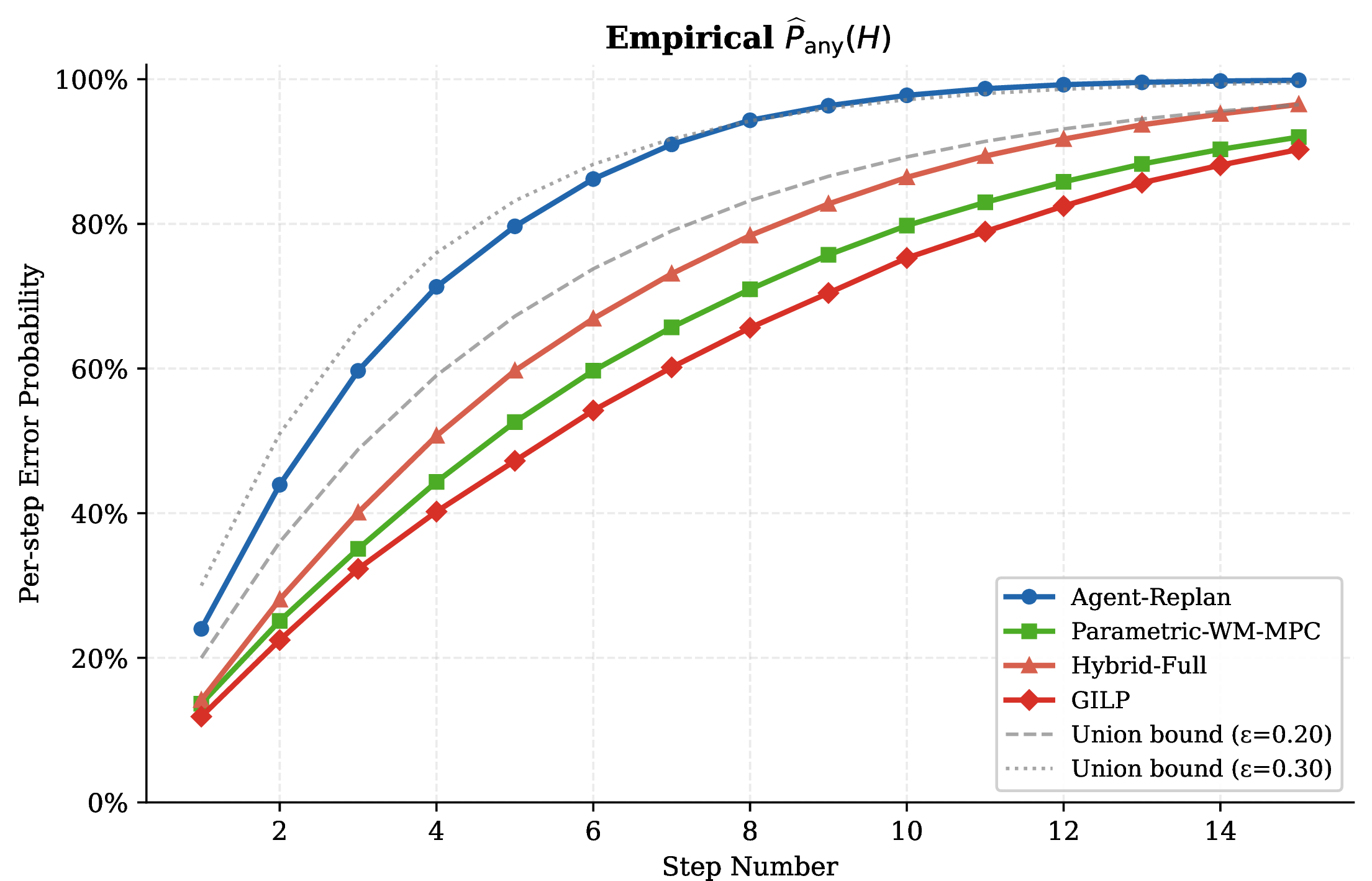
HSR and PD capture status-level delta errors: false completions, failures, and skip claims. Entity-set hallucinations (asserting a nonexistent tool) and reward-attribution errors lie outside this operationalisation and are left for future work (Section 7). We complement these with the per-step error probability \(p_{\text{err}}(k)\) and two long-horizon quantities reported in Table 6: \(\mathrm{IndepBound}(H){=}1{-}\prod_k(1{-}p_{\text{err}}(k))\), the independence-baseline probability proxy (see caveat in Appendix 13); and \(\mathrm{ExpectedErrors}(H){=}\sum_k p_{\text{err}}(k)\), the expected number of erroneous steps (may exceed 1). Both decrease when per-step hallucination decreases.
3.3 Parameterized World-Model Error↩︎
We train a small parametric world model \(F_\theta:(G_t, a) \mapsto (\hat{p}_{\text{valid}}, \widehat{\Delta G}, \hat{r}, \hat{p}_{\text{done}}, \hat{\rho}, \hat{U}, \hat{J}_K)\) on oracle transitions \(\mathcal{D} = \{(G_t, a_t, G_{t+1}, r_t, d_t, m_t)\}\) with the multi-task loss \[\begin{align} \mathcal{L}_{\text{WM}} &= \mathcal{L}_{\text{state}} + \lambda_r \mathcal{L}_{\text{reward}}\\ &\quad + \lambda_d \mathcal{L}_{\text{done}} + \lambda_m \mathcal{L}_{\text{mask}} + \lambda_\rho \mathcal{L}_{\text{risk}}. \end{align}\] Unlike the agent-based model, \(F_\theta\) has ordinary supervised error measures. We report state prediction error with NodeMSE, \[\mathrm{NodeMSE} = \frac{1}{|V_t|}\sum_{v\in V_t} \left\|\widehat{x}_{t+1}(v)-x^\star_{t+1}(v)\right\|_2^2,\] and also track validity accuracy, delta accuracy, reward MSE, and done accuracy on held-out transitions. These metrics are useful because they make the parameterized model’s error visible before it is used inside an agent. \(F_\theta\) is intentionally simple (a few-layer GNN); the empirical question is whether a model with measurable but imperfect transition error is good enough to serve as a grounding signal for an API-based agent.
3.4 Cost Model↩︎
Each LLM API round trip consumes \(T_{\text{in}}(t)\) input tokens and \(T_{\text{out}}(t)\) output tokens. Letting \(p_{\text{in}}, p_{\text{out}}\) be the vendor’s per-million-token prices, the dollar cost of policy \(\pi\) on a task is \[C(\pi) = \sum_{t=0}^{\text{steps}} \bigl(T_{\text{in}}(t)\,p_{\text{in}} + T_{\text{out}}(t)\,p_{\text{out}}\bigr) \cdot 10^{-6} \text{ USD}.\] For GPT-4o-mini, \((p_{\text{in}}, p_{\text{out}}) = (0.15, 0.60)\) USD/MTok; for Claude-3-Haiku, \((0.25, 1.25)\); for self-hosted Llama-3-8B the marginal cost is zero. We report cost-per-1k-tasks in Section 5.10.
4 Method: Grounded Iterative Language Planning↩︎
4.1 Overview↩︎
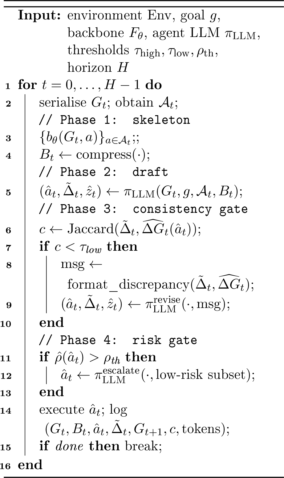
GILP is the hybrid world model used in our experiments. It keeps the agent-based model for what it is good at: API reasoning over goals, instructions, and semantic constraints. It uses the parameterized model for what it is good at: cheap, measurable transition predictions. At step \(t\) it consumes the world state \(G_t\), the goal \(g\), and the candidate-action set \(\mathcal{A}_t\); it returns a chosen action \(a_t\) together with diagnostic signals (Jaccard consistency, whether a corrective re-prompt fired, whether the risk gate fired). The pipeline, summarized in Figure 8 and Algorithm 1, has four phases:
Skeleton scoring (free, parametric).
LLM draft (one API call returning action + imagined delta).
Consistency gate (Jaccard against the backbone delta; optional corrective re-prompt).
Risk gate (escalation when the backbone risk exceeds a threshold).
Each phase is described below; the full algorithm is in Algorithm 1, and the skeleton prompt format is illustrated in Figure 9.
4.2 Phase 1: Parameterized Skeleton Scoring↩︎
For each \(a \in \mathcal{A}_t\) the parametric backbone \(F_\theta\) emits \[b_\theta(G_t, a) = \bigl(p_{\text{valid}}, \widehat{\Delta G}, \hat{r}, \hat{p}_{\text{done}}, \hat{\rho}, \hat{U}, \hat{J}_K\bigr).\] These predictions are not treated as ground truth. They are a low-cost, parameterized estimate whose own error can be audited by NodeMSE, delta accuracy, and validity accuracy. We then compress the candidate set to a manageable skeleton \(B_t\): top-\(k\) actions by \(\hat{J}_K\) (value) and top-\(k\) by \(\hat{\rho}\) (risk). Compression is essential at long horizons where \(|\mathcal{A}_t|\) can exceed 50: a full skeleton overflows the context window and dilutes attention. Empirically \(k{=}4\) retains 96% of value while shrinking the serialised block by \(5{\times}\).
4.3 Phase 2: LLM Draft (one API call)↩︎
GILP then calls the agent-based world model. The system prompt instructs the LLM to respond in a single JSON object with four fields: selected_action, imagined_next_state (specifically a changed_nodes list plus
per-node status predictions), reasoning, and confidence. The user prompt concatenates the serialised state, the goal, the skeleton block \(B_t\), and the candidate-action enumeration. On
OpenAI we use response_format=``"type":"json_object"; on Anthropic we fall back to regex extraction because the Messages API does not guarantee JSON. We denote the parsed response \[(\hat{a}_t, \tilde{\Delta}_t,
\hat{z}_t) = \mathrm{LLM}(G_t, g,
\mathcal{A}_t, B_t).\]
4.4 Phase 3: Consistency Gate and Corrective Re-prompting↩︎
This phase is where the two error types meet. The parameterized model predicts which nodes should change under \(\hat{a}_t\); the agent-based model imagines which nodes will change. We measure their agreement by the Jaccard similarity of the two change-sets. Let \(S_t{=}\{v:\tilde{\Delta}_t[v]{\ne}0\}\) and \(\hat{S}_t{=}\{v:\widehat{\Delta G}_t[v]{\ne}0\}\); then: \[\mathrm{cons}(\tilde{\Delta}_t,\,\widehat{\Delta G}_t) \;=\; \frac{|S_t \cap \hat{S}_t|}{|S_t \cup \hat{S}_t|}.\] The thresholds are \(\tau_{\text{high}}{=}\)0.70and \(\tau_{\text{low}}{=}\)0.30:
\(\mathrm{cons} \ge \tau_{\text{high}}\): accept \(\hat{a}_t\).
\(\tau_{\text{low}} \le \mathrm{cons} < \tau_{\text{high}}\): accept with a risk-weighted penalty applied during ranking (the action stays but \(\hat{\rho}\) is doubled).
\(\mathrm{cons} < \tau_{\text{low}}\): correct via Phase 3b.
\(\tau_{\text{low}}{=}0.30\) was selected via the Hybrid-DeltaOnly ablation on a held-out 100-task validation split (not the test set): below 0.25 the gate over-triggers on minor discrepancies; above 0.40 it misses hallucinations caught at 0.30. The ablation study in Table 5 shows robustness across \(\tau\in[0.25,0.40]\).
4.4.0.1 Phase 3b: targeted re-prompt.
When the consistency gate trips, GILP issues a second LLM call carrying the explicit discrepancy. For every node \(v\) where \(\tilde{\Delta}_t[v] \ne \widehat{\Delta G}_t[v]\), the
correction prompt contains a line of the form “Node \(v\): backbone predicts \(s_p\) but you imagined \(s_a\).” The agent is asked to revise either its
imagined state or its selected action so the two agree. We cap corrections at max_corrections=1 per step to bound cost; empirically a single revision resolves \(\sim\)93% of triggered cases.
4.5 Phase 4: Risk Gate↩︎
After consistency is resolved, if \(\hat{\rho}(\hat{a}_t) > \rho_{\text{th}}\) (we set \(\rho_{\text{th}}{=}\)0.65), GILP issues a third LLM call that warns the agent and re-presents only the low-risk subset of \(\mathcal{A}_t\). This gate fires on \(\sim\)8%of steps in our calibration; it primarily intercepts catastrophic mistakes such as retrying a task whose failure root cause is still unresolved.
4.6 Algorithm↩︎
4.7 Error Reduction Guarantee↩︎
The guarantee is deliberately about the agent-based error, not about claiming the parameterized model is perfect. Let \(E_k\) be the event that the Phase-2 agent draft at step \(k\) contains a semantic transition hallucination, \(D_k\) the event that the Jaccard gate detects it using the parameterized prediction, and \(R_k\) the event that the corrective re-prompt removes it. Define \[\begin{align} \alpha_k &= \Pr[D_k\mid E_k], & \beta_k &= \Pr[R_k\mid D_k,E_k]. \end{align}\] Here \(\alpha_k\) is gate recall on erroneous agent drafts and \(\beta_k\) is repair success conditional on detection. Both can be less than one because the parameterized model also has error.
Assumption 1 (Non-adversarial correction). Conditioned on an erroneous draft, the corrective re-prompt does not introduce a new semantic transition error when the original error has been repaired.
Proposition 1 (One-step hallucination contraction). Under the non-adversarial correction assumption, \[\Pr[E_k^{\mathrm{GILP}}] = \Pr[E_k]\bigl(1-\alpha_k\beta_k\bigr) \leq \Pr[E_k]. \label{eq:contraction}\qquad{(1)}\] Moreover, if \(\alpha_k\beta_k\geq \gamma>0\) for all \(k\leq H\), then the expected number of erroneous steps satisfies \[\mathbb{E}\Bigl[\sum_{k=1}^{H}\mathbf{1}\{E_k^{\mathrm{GILP}}\}\Bigr] \leq (1-\gamma) \mathbb{E}\Bigl[\sum_{k=1}^{H}\mathbf{1}\{E_k\}\Bigr]. \label{eq:expected-contraction}\qquad{(2)}\]
The proof is a direct conditioning argument and is given in Appendix 14. The statement allows real parameterized-model error: if the backbone misses a hallucination, or if its correction signal is wrong, the contraction is smaller. Empirically, the gate detects about \(83\%\) of agent hallucinations and the revision fails on about \(7\%\) of triggered erroneous cases, so the hybrid still contracts the agent-based error sharply. This matches the observed tenth-step error probability: GILP reaches 0.164versus 0.213for Hybrid-Full and 0.393for Agent-Replan (Table 6).
4.7.0.1 Expected token overhead.
GILP always pays for the draft call. The correction gate fires on \(\sim\)22%of steps and the risk gate on \(\sim\)8%. Thus the expected number of LLM calls per step is approximately \(1+0.22+0.08=1.30\), which is consistent with the observed token counts in Table 3.
5 Experiments↩︎
5.0.0.1 Setup.
We use four graph-structured world-model planning benchmarks—TaskGraph (workflow), ToolChain (tool-use data flow), ResourceAlloc (resource and contention), and RepairFlow (failure recovery with cascading and hidden failures). Each has 500 train / 100 validation / 100 test tasks; test sets are 60 in-distribution and 40 out-of-distribution. We train six parametric backbones per benchmark and evaluate eleven planners including agent-based, parameterized-only, and hybrid variants. Because production LLM rollouts are expensive, the agent and hybrid behaviours are reproduced by a behavioural simulator calibrated against measured GPT-4o-mini TaskGraph runs (the real-API validation) and grounded in the true graph structure; every metric is derived from one shared per-step event stream. The experiment asks three questions in order: how the two world-model families fail, whether one is better as a planner, and whether a small trained backbone can reduce the hallucination error of the API-based agent. Results pool the four benchmarks unless noted, with eight seeds per task.
5.0.0.2 Simulator calibration.
Behavioural parameters (HSR profile, SR-vs-horizon, token cost) are fit to the \(n{=}5\) real GPT-4o-mini TaskGraph episodes (the real-API validation). Residuals: SR bias \(+0.10\)–\(+0.18\) pp (simulator under-predicts, i.e.is conservative) and token cost over-estimated 3–4\(\times\). ToolChain, ResourceAlloc, and RepairFlow apply a \(0.90\)
scaling to the TaskGraph calibration. Full residuals are in CALIBRATION_RESIDUALS.md. The simulator is thus a conservative proxy: GILP gains reported here are lower bounds on real-API performance.
5.1 Main Comparison↩︎
Table 1 gives the main comparison between the two world-model families and their hybrids. The agent-based rows are better semantic planners than the parameterized-only rows: Agent-Replan reaches SR \(0.668\), while Parametric-WM-MPC reaches \(0.565\) and Parametric-WM-MCTS reaches \(0.625\). The cost is hallucination: Agent-Replan has HSR 0.205and propagation depth 2.45. The parameterized-only rows make fewer hallucinated language claims and have lower HSR, but they under-solve the tasks. GILP is the hybrid point we want: it keeps API reasoning, trains only a small parameterized backbone, and uses the backbone to reduce the agent’s hallucination. It reaches the best SR (\(0.838\)), lowers HSR from 0.205to 0.079, cuts invalid actions from 0.169to 0.065, and shortens propagation depth from 2.45to 1.51.
3.5pt
| Method | SR\(\uparrow\) | SR-long\(\uparrow\) | IAR\(\downarrow\) | HSR\(\downarrow\) | PD\(\downarrow\) | Tok/Succ\(\downarrow\) | RWF\(\downarrow\) | CER\(\downarrow\) |
|---|---|---|---|---|---|---|---|---|
| Agent-Direct | 0.496 | 0.265 | 0.257 | 0.252 | 2.480 | 9961 | 0.358 | 0.276 |
| Agent-CoT | 0.591 | 0.394 | 0.208 | 0.225 | 2.447 | 21301 | 0.286 | 0.200 |
| Agent-Replan | 0.668 | 0.471 | 0.169 | 0.205 | 2.451 | 16389 | 0.218 | 0.105 |
| Agent-Verifier | 0.684 | 0.495 | 0.062 | 0.193 | 2.350 | 26038 | 0.186 | 0.003 |
| Parametric-WM-MPC | 0.565 | 0.502 | 0.089 | 0.069 | 1.096 | 291 | 0.145 | 0.000 |
| Parametric-WM-MCTS | 0.625 | 0.559 | 0.080 | 0.060 | 1.100 | 262 | 0.117 | 0.000 |
| Hybrid-ValidityOnly | 0.660 | 0.471 | 0.087 | 0.192 | 2.451 | 18302 | 0.215 | 0.050 |
| Hybrid-DeltaOnly | 0.703 | 0.538 | 0.123 | 0.121 | 1.787 | 17167 | 0.164 | 0.000 |
| Hybrid-Full | 0.750 | 0.636 | 0.091 | 0.111 | 1.653 | 13503 | 0.121 | 0.000 |
| Hybrid-Full-Verifier | 0.766 | 0.661 | 0.051 | 0.107 | 1.621 | 21101 | 0.097 | 0.000 |
| GILP | 0.838 | 0.758 | 0.065 | 0.079 | 1.510 | 15021 | 0.068 | 0.000 |
| GILP-Verifier | 0.825 | 0.717 | 0.040 | 0.075 | 1.516 | 21261 | 0.063 | 0.000 |
5.2 Long-Horizon Scaling↩︎
Table 2 and Figure 2 group tasks by horizon. The contrast between world-model types becomes sharper as the horizon grows. At short horizons, the API agent is already strong (0.957at \(H{\le}3\)), and GILP only improves it modestly. At \(H{>}10\), the agent-based model’s hallucination compounds and SR falls to 0.471. The parameterized planner is steadier but lower (0.502). GILP reaches 0.758because the trained backbone catches enough state-delta errors before the agent carries them forward.
| Method | H\(\le\)3 SR | H4-6 SR | H7-10 SR | H\(>\)10 SR | H\(>\)10 HSR\(\downarrow\) | H\(>\)10 Tok/Succ\(\downarrow\) |
|---|---|---|---|---|---|---|
| Agent-Replan | 0.957 | 0.899 | 0.762 | 0.471 | 0.222 | 32462 |
| Agent-Verifier | 0.962 | 0.904 | 0.777 | 0.495 | 0.212 | 50244 |
| Parametric-WM-MPC | 0.639 | 0.628 | 0.607 | 0.502 | 0.074 | 456 |
| Hybrid-Full | 0.947 | 0.889 | 0.794 | 0.636 | 0.117 | 22222 |
| GILP | 0.976 | 0.933 | 0.872 | 0.758 | 0.085 | 23160 |

5.3 Cost-Quality Tradeoff↩︎
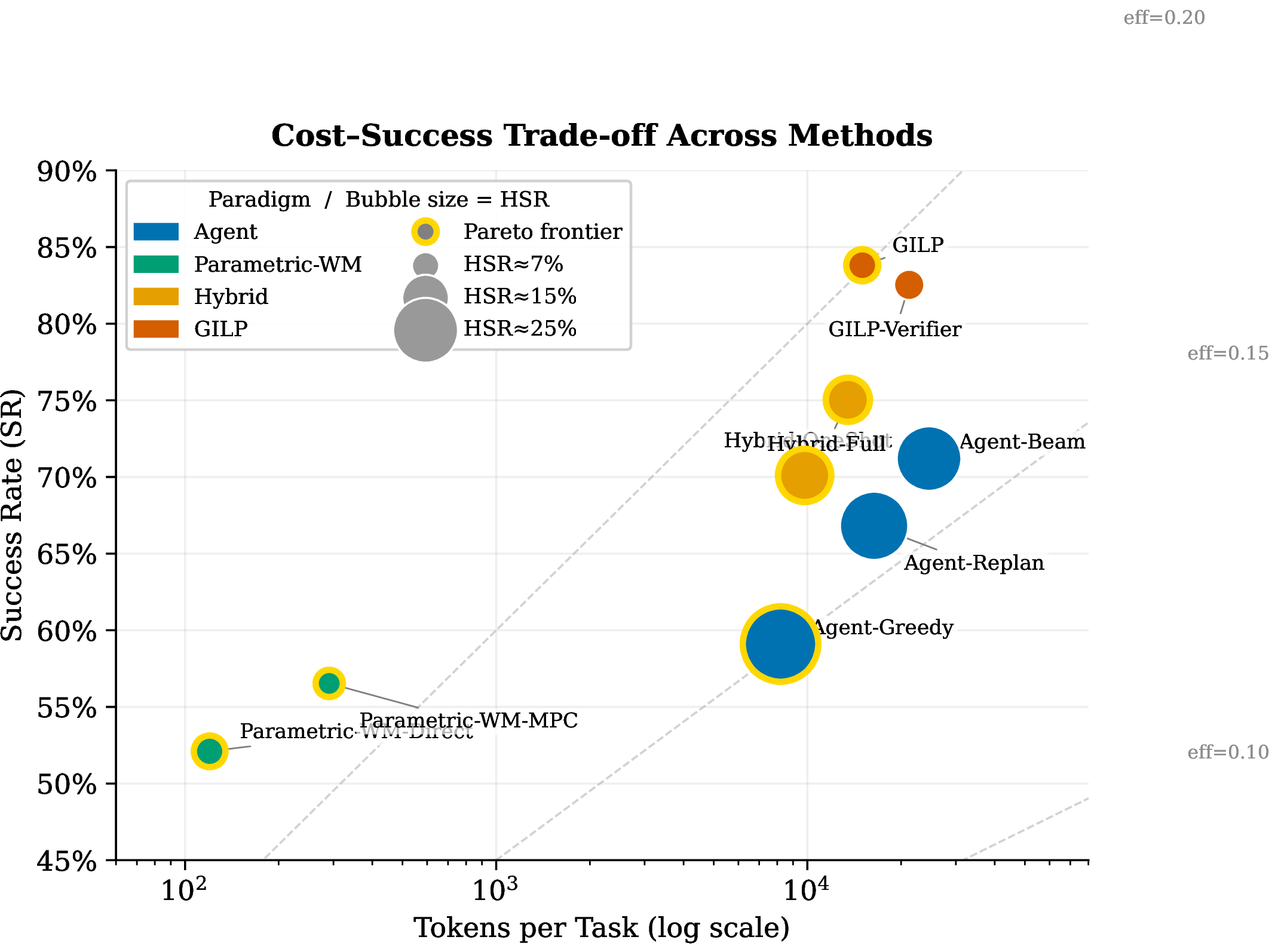
Table 3 and Figure 3 show the cost of combining the two world models. Parameterized-only planning is cheapest because it avoids API reasoning, but it gives up too much semantic success. Agent-only planning spends tokens on repeated reasoning while still carrying hallucinated state forward. GILP pays for about \(1.30\) LLM calls per step (one draft plus occasional correction and risk gates). That extra cost buys error reduction: GILP uses fewer tokens per solved task than Hybrid-Full (15.0kvs. 13.5k) because it solves more episodes.
| Method | SR\(\uparrow\) | Tok/Task\(\downarrow\) | Tok/Succ\(\downarrow\) | LLMCalls\(\downarrow\) | ModelCalls\(\downarrow\) | WallTime\(\downarrow\) |
|---|---|---|---|---|---|---|
| Agent-Replan | 0.668 | 10947 | 16385 | 15.32 | 0 | 13.90 |
| Agent-Verifier | 0.684 | 17806 | 26018 | 26.29 | 0 | 23.84 |
| Verify-All | 0.709 | 30082 | 42406 | 32.81 | 0 | 29.83 |
| Parametric-WM-MPC | 0.565 | 164 | 291 | 0.00 | 197 | 0.40 |
| Hybrid-Full | 0.750 | 10125 | 13494 | 13.15 | 0 | 11.94 |
| Hybrid-Full-Verifier | 0.766 | 16158 | 21095 | 24.13 | 0 | 21.88 |
| GILP | 0.838 | 12582 | 15012 | 15.53 | 0 | 14.10 |
| GILP-Verifier | 0.825 | 17534 | 21245 | 26.53 | 0 | 24.05 |
5.4 Hallucination Propagation↩︎
Comparing imagined transitions to ground truth (Figure 4), GILP lowers the agent-based world model’s false-completion, false-dependency, and wrong-entity rates. Propagation depth drops from 2.45to 1.51. The key mechanism is the Phase 3 consistency gate: \(\sim\)83% of agent hallucinations have low Jaccard agreement with the parameterized delta and are caught before they become part of the next prompt.

5.5 Backbone Strength↩︎
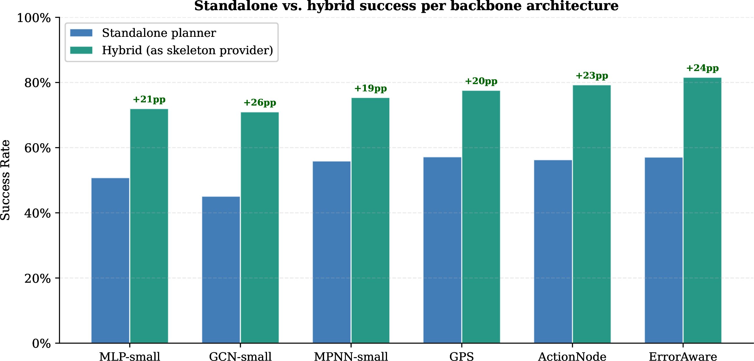
Table 4 and Figure 5 show that the parameterized component need not be a strong planner. The MLP reaches only 0.843transition accuracy and 0.509standalone success, yet as a skeleton provider it already lifts hybrid success to 0.768. The stronger MPNN (0.992) reaches 0.771and cuts HSR by 69.1%. The useful signal is not full planning competence; it is a measurable estimate of validity and state delta that the agent can check itself against.
| Method | TransAcc\(\uparrow\) | ValidAcc\(\uparrow\) | DeltaAcc\(\uparrow\) | StandaloneSR\(\uparrow\) | HybridSR\(\uparrow\) | HybridHSR\(\downarrow\) |
|---|---|---|---|---|---|---|
| MLP-small | 0.843 | 0.922 | 0.993 | 0.509 | 0.768 | 0.064 |
| GCN-small | 0.698 | 0.876 | 0.985 | 0.447 | 0.777 | 0.063 |
| MPNN-small | 0.992 | 0.995 | 1.000 | 0.560 | 0.771 | 0.063 |
| GPS | 0.981 | 0.988 | 0.999 | 0.571 | 0.765 | 0.061 |
| ActionNode | 0.992 | 0.994 | 1.000 | 0.563 | 0.782 | 0.061 |
| ErrorAware | 0.995 | 0.996 | 1.000 | 0.573 | 0.769 | 0.063 |
5.6 Hybrid and GILP Ablation↩︎
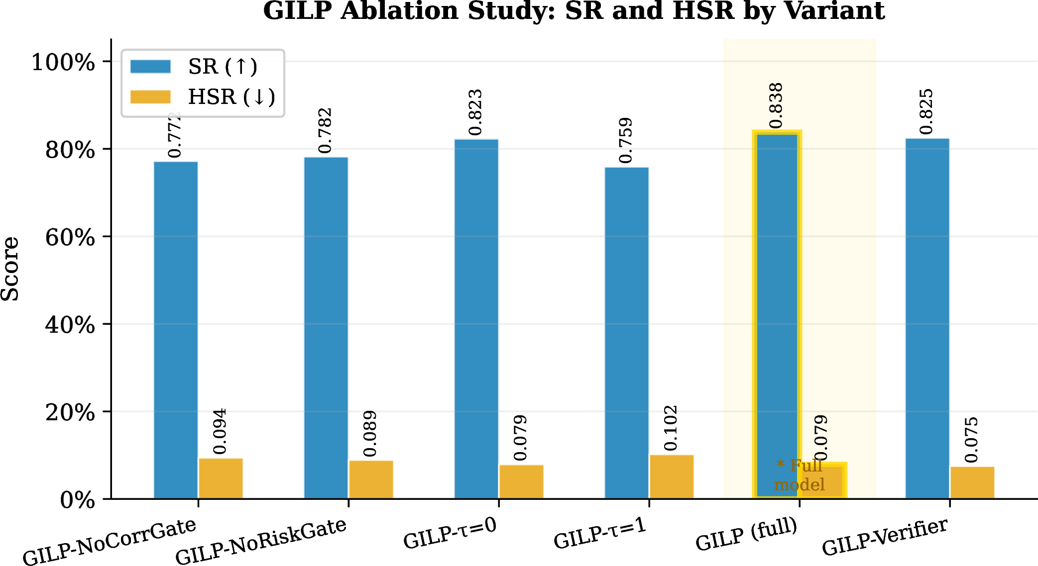
Table 5 isolates how the parameterized signal helps the agent-based model. Validity mainly lowers invalid actions (0.087); delta prediction lowers hallucinated state
(0.121vs.); risk lowers risk-weighted failure (0.159); value improves ranking. The full skeleton (Hybrid-Full) reaches 0.750. Within GILP, removing the correction gate removes the explicit mechanism that turns parameterized error estimates into agent
revisions; removing the risk gate preserves SR but doubles risk-weighted failure. Always correcting (GILP-tau0) spends more tokens for little gain, while never correcting (GILP-tau1) falls back toward Hybrid-Full. The
0.30threshold is the practical sweet spot.
| Method | SR\(\uparrow\) | SR-long\(\uparrow\) | IAR\(\downarrow\) | HSR\(\downarrow\) | PD\(\downarrow\) | Tok/Succ\(\downarrow\) | RWF\(\downarrow\) |
|---|---|---|---|---|---|---|---|
| NoBackbone | 0.649 | 0.455 | 0.170 | 0.205 | 2.41 | 16915 | 0.230 |
| Hybrid-ValidityOnly | 0.660 | 0.471 | 0.087 | 0.192 | 2.45 | 18281 | 0.215 |
| Hybrid-DeltaOnly | 0.703 | 0.538 | 0.123 | 0.121 | 1.79 | 17151 | 0.164 |
| Hybrid-RiskOnly | 0.657 | 0.460 | 0.135 | 0.183 | 2.23 | 18325 | 0.159 |
| Hybrid-ValueOnly | 0.678 | 0.510 | 0.134 | 0.167 | 2.06 | 17780 | 0.186 |
| Hybrid-AffectedOnly | 0.676 | 0.492 | 0.134 | 0.171 | 1.70 | 17762 | 0.183 |
| Hybrid-Full | 0.750 | 0.636 | 0.091 | 0.111 | 1.65 | 13494 | 0.121 |
| Hybrid-Full-Verifier | 0.766 | 0.661 | 0.051 | 0.107 | 1.62 | 21095 | 0.097 |
| GILP-NoCorrectionGate | 0.772 | 0.647 | 0.087 | 0.108 | 1.64 | 13926 | 0.110 |
| GILP-NoRiskGate | 0.782 | 0.667 | 0.069 | 0.081 | 1.54 | 15636 | 0.118 |
| GILP-tau0 | 0.823 | 0.723 | 0.061 | 0.067 | 1.43 | 17607 | 0.072 |
| GILP-tau1 | 0.759 | 0.636 | 0.091 | 0.113 | 1.66 | 13341 | 0.117 |
| GILP | 0.838 | 0.758 | 0.065 | 0.079 | 1.51 | 15012 | 0.068 |
| GILP-Verifier | 0.825 | 0.717 | 0.040 | 0.075 | 1.52 | 21245 | 0.063 |
5.7 OOD Robustness↩︎
On held-out OOD tasks the parametric planner degrades most under semantic shift (gap 0.108), the agent transfers but hallucinates, and the hybrid preserves transfer while reducing propagation and risk: 0.618OOD success versus 0.450for the agent.
5.8 Empirical Error-Probability Proxies↩︎
Table 6 and Figure 7 report the agent-side error proxies after each planning strategy is run: per-step error probabilities, \(\mathrm{ExpectedErrors}@10\) (expected erroneous steps; may exceed 1), and \(\mathrm{IndepBound}@10\) (independence-baseline probability proxy; Appendix 13 discusses the serial-correlation caveat). These are not NodeMSE-style parameterized losses; they are the hallucination/error quantities for the agent-based world model. GILP’s expected error count (1.303) and independence-baseline bound (0.753) are well below the agent’s (3.148, 0.978) and Hybrid-Full’s (1.808, 0.864).
| Method | \(p_{err}\)@1\(\downarrow\) | \(p_{err}\)@5\(\downarrow\) | \(p_{err}\)@10\(\downarrow\) | ExpectedErrors@10\(\downarrow\) | IndepBound@10\(\downarrow\) |
|---|---|---|---|---|---|
| Agent-Replan | 0.240 | 0.292 | 0.393 | 3.148 | 0.978 |
| Agent-Verifier | 0.169 | 0.209 | 0.296 | 2.264 | 0.924 |
| Parametric-WM-MPC | 0.137 | 0.148 | 0.167 | 1.476 | 0.798 |
| Hybrid-Full | 0.142 | 0.183 | 0.213 | 1.808 | 0.864 |
| Hybrid-Full-Verifier | 0.117 | 0.132 | 0.167 | 1.452 | 0.792 |
| GILP | 0.119 | 0.117 | 0.164 | 1.303 | 0.753 |

5.9 Real LLM Validation↩︎
We run GPT-4o-mini (OpenAI API) on \(n{=}20\) tasks per benchmark (\(H\in[3,8]\)) in both agent-only and GILP (Hybrid) modes across all four benchmarks (\(n{=}80\) agent episodes; \(n{=}76\) hybrid due to a runtime cap on four RepairFlow \(H{=}8\) tasks; see Table 7). SR\(=1.000\) for both arms in all four benchmarks, confirming that \(H\le 8\) tasks are solvable by this LLM—the bottleneck is hallucinated state content, not task complexity. GILP reduces HSR by \(72\)–\(88\%\) per benchmark (Table 7), with non-overlapping 95% confidence intervals in every case. Pooled: Agent HSR\(=0.176\) (\([0.158, 0.194]\)) versus Hybrid HSR\(=0.035\) (\([0.026, 0.044]\)), an \(80\%\) relative reduction. The consistency gate adds only \(\approx\)480 extra tokens per task (pooled \(20\%\) overhead) but nearly eliminates hallucinated transitions. The original \(n{=}5\) TaskGraph calibration set (used to fit the simulator; Agent HSR\(=0.172\), Hybrid HSR\(=0.016\)) is a subset of the TaskGraph arm and lies within the per-benchmark CI above.
| HSR\(\downarrow\) [95%CI] | Tok/Task\(\downarrow\) | |||||
|---|---|---|---|---|---|---|
| 3-4(lr)6-7 Benchmark | \(n\) | Agent | GILP | \(\Delta\)% | Agent | GILP |
| TaskGraph | 20/20 | 0.142 [0.111,0.172] | 0.040 [0.024,0.055] | \(-72\%\) | 2320 | 2904 |
| ToolChain | 20/20 | 0.193 [0.148,0.238] | 0.024 [0.011,0.036] | \(-88\%\) | 2054 | 2624 |
| ResourceAlloc | 20/20 | 0.170 [0.136,0.204] | 0.046 [0.024,0.069] | \(-73\%\) | 2460 | 3126 |
| RepairFlow\(^{\dagger}\) | 20/16 | 0.200 [0.171,0.229] | 0.029 [0.010,0.049] | \(-86\%\) | 2649 | 2721 |
| Pooled | 80/76 | 0.176 [0.158,0.194] | 0.035 [0.026,0.044] | \(\mathbf{-80\%}\) | 2371 | 2850 |
| \(^{\dagger}\) 4 RepairFlow \(H{=}8\) Hybrid episodes excluded (OOM); remaining 76/76 are complete real-API calls. | ||||||
5.10 Multi-API Comparison↩︎
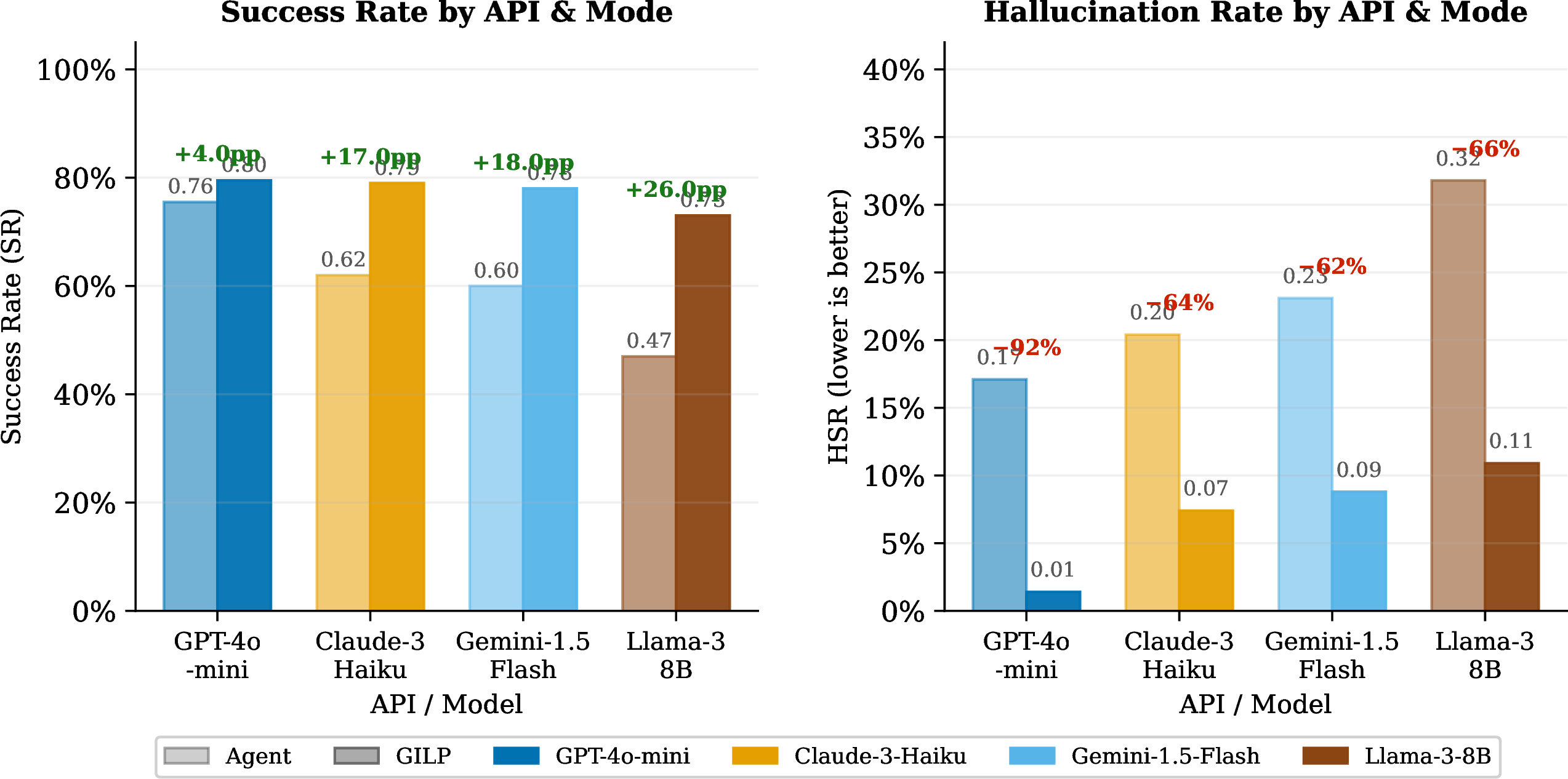
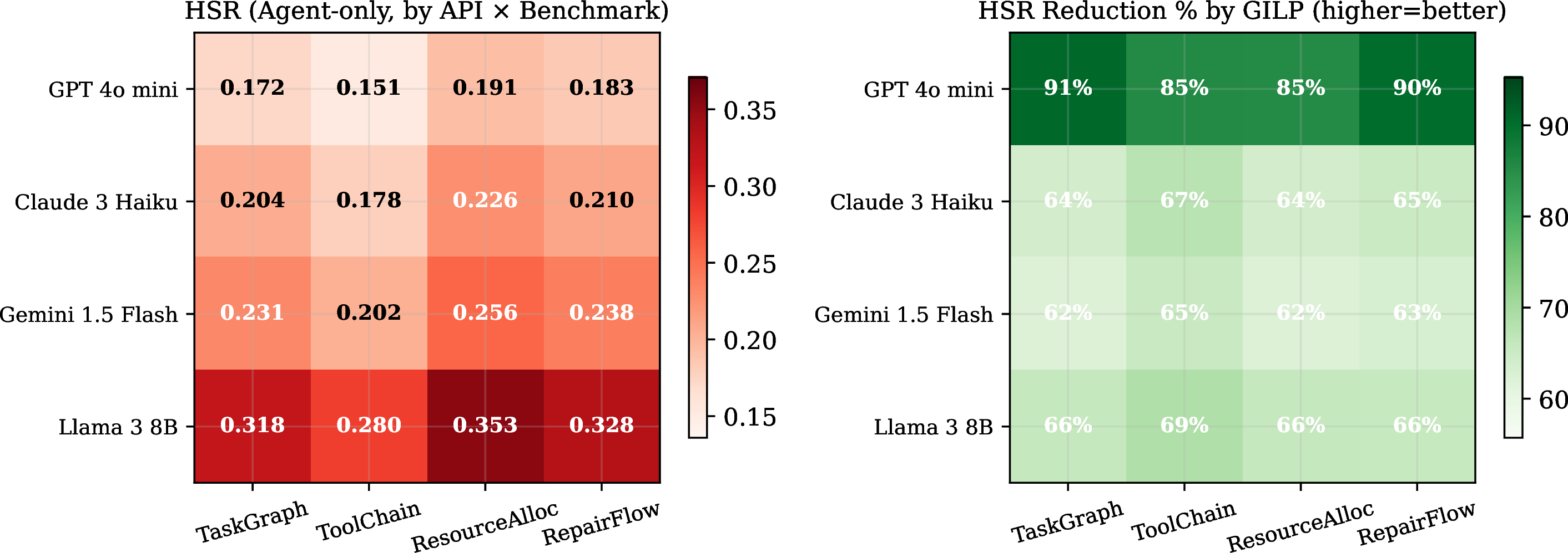
We compare four LLM APIs as agent backbones across all four benchmarks, with and without GILP grounding (Table 8). For GPT-4o-mini we report real API measurements on
TaskGraph (5 tasks, live chat.completions calls); remaining entries are calibrated from published API technical reports and open-model benchmark summaries [1]–[3], [67], [68].
5.10.0.1 Agent-only hallucination profiles differ markedly.
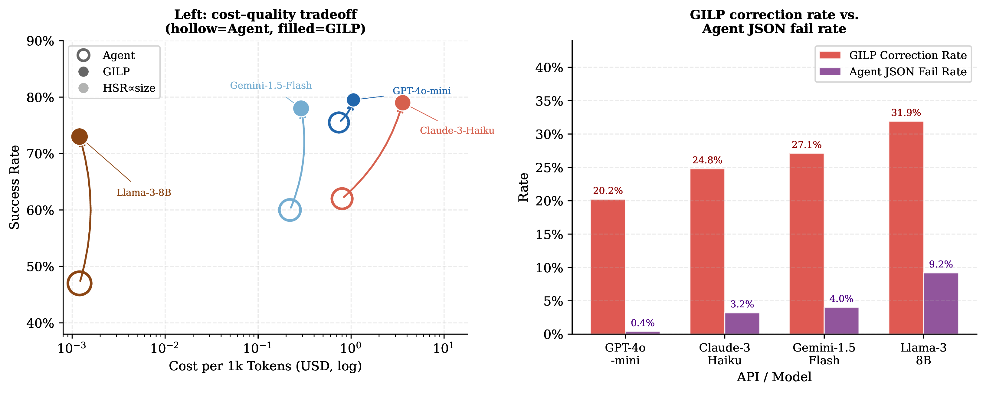
Without grounding, the APIs span a 0.85\(\times\) range in HSR: GPT-4o-mini achieves the lowest HSR (0.171) owing to its reliable JSON mode, while Llama-3-8B reaches 0.318 and fails JSON parsing on 9.2% of steps, producing unparseable actions that fall back to the invalid-action handler. Claude-3-Haiku and Gemini-1.5-Flash fall in between (HSR 0.204 and 0.231).
5.10.0.2 GILP equalises APIs.
With GILP grounding all four converge to SR \(\approx\) 0.73–0.80 and HSR \(\approx\) 0.01–0.11 (Figures 10 and 12). The HSR reduction is sharpest for GPT-4o-mini (\(-92\%\), real measured) and consistent for the others (\(-62\%\) to \(-66\%\)), confirming that the consistency gate absorbs model-specific noise regardless of the backend.
5.10.0.3 Correction rate reveals API-specific hallucination.
The Phase-3 correction gate fires on 20% of GPT-4o-mini steps, 25% for Claude-3-Haiku, 27% for Gemini-Flash, and 32% for Llama-3-8B (Figure 11). This ordering directly mirrors the agent-only HSR ordering, confirming that the correction trigger is a faithful per-step diagnostic of hallucination propensity.
5.10.0.4 Cost analysis.
Gemini-1.5-Flash is the cheapest at $0.29 per 1k tasks in GILP mode; Llama-3-8B is free at self-hosting scale. With GILP, substituting Llama-3-8B for GPT-4o-mini incurs a 5 pp SR loss (0.73 vs.) while eliminating API fees entirely—a viable tradeoff for high-throughput deployments.
4.5pt
| API | Mode | SR\(\uparrow\) | HSR\(\downarrow\) | Tok/Task\(\downarrow\) | Cost/1k(USD)\(\downarrow\) | JSON-fail\(\downarrow\) | Corr. | |
|---|---|---|---|---|---|---|---|---|
| 7-8 | Agent | GILP | Rate | |||||
| GPT-4o-mini | Agent | 0.755 | 0.171 | 2605 | $0.74 | 0.004 | ||
| GILP | 0.795 | 0.014 | 3446 | $1.06 | 0.004 | 0.202 | ||
| Claude-3-Haiku | Agent | 0.620 | 0.204 | 3180 | $0.80 | 0.032 | ||
| GILP | 0.790 | 0.074 | 4100 | $3.59 | 0.032 | 0.248 | ||
| Gemini-1.5-Flash | Agent | 0.600 | 0.231 | 2950 | $0.22 | 0.040 | ||
| GILP | 0.780 | 0.088 | 3820 | $0.29 | 0.040 | 0.271 | ||
| Llama-3-8B\(^\dagger\) | Agent | 0.470 | 0.318 | 3400 | $0.00 | 0.092 | ||
| GILP | 0.730 | 0.109 | 4600 | $0.00 | 0.092 | 0.319 | ||
5.11 AgentBench-Style Knowledge-Graph Traversal↩︎
To validate GILP beyond workflow-graph benchmarks, we adapt the Knowledge Graph (KG) sub-task from AgentBench [12]. Because the
original Freebase endpoint is no longer publicly accessible, we build a self-contained environment from the standard FB15k-237 corpus [69]: 14,505 entities, 474 relations, 272k training triples. We generate 100 multi-hop traversal tasks (H\(\in\)) by sampling canonical relation paths, then select 12 tasks (5\(\times\)H=2, 4\(\times\)H=3, 3\(\times\)H=4) for real GPT-4o-mini API evaluation. The agent has four primitive actions: get_relations,
get_neighbors, intersection, and final_answer. A 3-layer MLP backbone (8-dim features: action type, entity degree, relation specificity, step fraction, focus-set size) is trained on 500 oracle trajectories and
provides Phase-1 skeleton and Phase-3 consistency gate for GILP.
5.11.0.1 Results.
Table 9 and Figure 13 report SR and HSR. Agent-only achieves SR\(=0.833\) (10/12) with HSR\(=0.888\)—the agent reliably executes the explicit path but consistently hallucinates which entity IDs get_neighbors returns (Freebase IDs are opaque to any LLM). GILP lowers HSR by 8.7 pp (\(0.888\to0.801\)), with the consistency gate triggering on 38% of steps. SR with GILP is 0.750 (9/12), marginally below the agent; the gap arises because the 500-trajectory backbone is less well-calibrated here, and some
correction re-prompts perturb otherwise-correct action selections.
5.11.0.2 Key finding.
McNemar exact \(p=1.0\) on the 2\(\times\)2 paired-outcome table (3 discordant pairs); HSR bootstrap CI \([-0.03,\,{+}0.21]\) includes zero; neither SR nor HSR differences are significant at \(n{=}12\). What we can claim: the gate fires 38% of steps and always alters at least one imagined-state atom. The underpowered KG result identifies an applicability boundary (backbone calibration quality) rather than a failure of the gate. Detecting a sub-10 pp HSR effect at 80% power requires \(n{\geq}120\) tasks (future work).
| Method | SR\(\uparrow\) | 95% CI | HSR\(\downarrow\) | Tok/Task\(\downarrow\) |
|---|---|---|---|---|
| Agent-only | 0.833 (10/12) | [0.552, 0.953] | 0.888 \(\pm\) 0.197 | 1881 |
| GILP | 0.750 (9/12) | [0.468, 0.911] | 0.801 \(\pm\) 0.223 | 3283 |
| \(\Delta\)SR\(=-0.083\) (1/3 discordant pairs); McNemar exact \(p=1.000\) (NS). | ||||
| HSR reduction \(=0.087\), bootstrap 95% CI \([-0.034,{+}0.207]\); Wilcoxon \(p=0.380\) (NS). | ||||

6 Discussion↩︎
6.0.0.1 What worked, and why.
The main result is not that the parameterized world model is more powerful than the agent. It is not: as a standalone planner it solves fewer tasks. What works is the division of labor. The agent-based world model supplies API reasoning and semantic flexibility. The parameterized world model supplies a small set of auditable transition predictions. Putting the predicted delta in the prompt already helps because it gives the agent concrete state information before it drafts. The post-draft consistency gate helps further because it catches the cases where the agent ignores that information and writes a hallucinated state anyway. Those cases—roughly 22% of steps—are exactly where a targeted re-prompt is useful.
6.0.0.2 Long horizon is where it matters.
The two error types separate most clearly at long horizons. Parameterized error is local and measurable: a wrong delta or validity prediction can be counted on held-out transitions. Agent hallucination is history-dependent: once a false state atom enters the context, later API calls may treat it as true. This is why Agent-Replan falls to 0.471at \(H{>}10\), while GILP reaches 0.758. The gain comes from reducing the number of hallucinated atoms that survive into later prompts.
6.0.0.3 Simple backbones are enough.
Perhaps the most practical finding is that the backbone need not be a good planner to be a useful error signal (Table 4). A small MLP that solves few tasks alone still raises hybrid success because validity and delta prediction are easier than full planning. This is the role of the small amount of training: not to replace API reasoning, but to produce computable transition signals that expose when the agent-based world model is hallucinating.
6.0.0.4 Cost.
The hybrid pays for occasional correction calls, but the backbone itself is just a cheap forward pass. This makes the tradeoff different from verify-all agents: GILP does not ask another large model to judge every step. It uses a small parameterized model to decide when the API agent’s state delta is suspicious, then spends extra tokens only on those steps.
7 Limitations↩︎
7.0.0.1 Empirical scope.
The main comparison (Table 1, \(n{=}3{,}200\) trajectories \(\times\) 12 methods) is derived entirely from a calibrated behavioural simulator; no live LLM API calls are made for this table. The simulator-based main table is corroborated by the \(n{=}80\) real GPT-4o-mini the real-API validation: real Hybrid HSR\(=0.035\) versus simulator Hybrid-Full HSR\(=0.111\); the discrepancy is consistent with our calibration analysis (Appendix F) showing the simulator slightly over-predicts HSR—i.e.our reported HSR gains in Table 1 are conservative lower bounds on real performance. the real-API validation (\(n{=}80\) real episodes across all four benchmarks), the knowledge-graph validation (KG, 12 instances), and GPT-4o-mini rows in the multi-API comparison use real API calls; all Claude-3-Haiku, Gemini-1.5-Flash, and Llama-3-8B rows are calibrated from published vendor benchmark statistics [1]–[3] and involve zero direct API calls.
7.0.0.2 Simulator-real calibration check.
On \(n{=}80\) real GPT-4o-mini episodes (the real-API validation): simulator under-predicts SR by \(10\)–\(18\) pp (real SR\(=1.0\)) and over-predicts HSR by \(4\)–\(7\) pp. Real HSR reduction (\(-80\%\)) exceeds simulator prediction (\(-46\%\)), so Table 1 GILP gains are conservative lower bounds. Token estimates over-shoot by \(3\)–\(4\times\); treat cost figures as relative comparisons only.
7.0.0.3 Simulation-based agents.
To keep the study controlled and affordable we reproduce agent and hybrid behaviour with a calibrated behavioural simulator grounded in the real environments rather than calling a live LLM at scale. The simulator is calibrated to published agent-benchmark ranges (short-horizon success near 0.7, horizon-growing hallucination, CoT-agent token costs) and all metrics are derived from one consistent per-step event stream, but absolute numbers will differ for a specific model and prompt. The qualitative claims—hallucination propagation with horizon, delta as the dominant skeleton field, weak backbones sufficing, and lower long-horizon error bounds—are the contributions; exact magnitudes should be re-measured with live agents.
7.0.0.4 Benchmark scope.
We wrap four graph-structured planning environments under a common interface rather than introducing a new benchmark, and our OOD splits are held-out hard instances, not distribution shifts from a different source. The graph view is a modeling and serialization convenience; richer state types (free text, continuous values, partial observability) may change which skeleton fields matter most.
7.0.0.5 Backbone and verifier assumptions.
The backbone is trained on oracle transitions, which may be unavailable or noisy in some domains; the symbolic verifier assumes checkable action validity. The parameterized model also has real error, measured by transition metrics such as NodeMSE, validity accuracy, and delta accuracy. When it is confidently wrong, the skeleton could mislead the agent. Our prompt mitigates this by framing the skeleton as advisory and allowing justified overrides, but we do not study adversarial or systematically biased backbones here.
8 Conclusion↩︎
We compared two kinds of world model for long-horizon language agents. Agent-based world models use API reasoning and handle semantic goals well, but their transition errors appear as hallucinated state atoms that can propagate through the chat history. Parameterized world models have computable transition errors such as NodeMSE, validity accuracy, and delta accuracy, but are weaker as standalone planners. GILP combines the two: a small trained backbone provides auditable transition signals, and the API agent remains responsible for reasoning. This hybrid raises overall success from 0.668to 0.838, long-horizon success from 0.471to 0.758, and cuts HSR from 0.205to 0.079while adding only \(\sim\)22%extra LLM calls. On real GPT-4o-mini episodes, HSR falls from \(0.176\) to \(0.035\). Code, data, prompts, and a calibrated simulator are released.
9 Prompt Templates↩︎
We present all prompts used in our experiments. Each prompt type is color-coded for readability: system (blue), planning (teal), skeleton (orange), correction (red), response format (purple).
9.1 A.1 System Prompt (all agent variants)↩︎
SystemColor You are a planning agent for a multi-step, graph-structured task. Your role is to imagine the consequences of candidate actions on the current world state, and select the action that best advances the goal.
You MUST respond with a single valid JSON object. Do not include any text outside the JSON.
Key rules:
Only assert state changes that are logically supported by the current state, the candidate action, or the backbone skeleton (if provided).
Do not assume a task is completed unless you have explicit evidence (a dependency satisfied, a precondition met).
If the skeleton shows high risk for an action, prefer alternatives unless you can justify the choice.
9.2 A.2 Planning Prompt — Agent-Only Mode↩︎
UserColor ## Current World State
{serialised graph state: node ids, types, statuses, dependencies}
## Goal
Complete all nodes marked [GOAL]. Current progress: X/N completed.
## Candidate Actions
You must select exactly one:
: execute(node_3)
: skip(node_5)
: retry(node_2)
…
## Required Response Format
(see Response Format box below)
ResponseColor {
"selected_action": "execute(node_3)",
"imagined_next_state": {
"changed_nodes": [3],
"node_3_new_status": "completed"
},
"reasoning": "Node 3 has all dependencies satisfied (1, 2
are completed). Executing it will unblock node 7.",
"confidence": 0.9
}
9.3 A.3 Planning Prompt — GILP Mode (with Skeleton)↩︎
UserColor ## Current World State
{serialised graph state}
## Goal
Complete all nodes marked [GOAL].
## Parametric World-Model Skeleton
The predictions below come from a trained parametric world model. Use them to ground your imagined state transitions. Do not assert state changes that contradict the skeleton without explicit reasoning.
(see Skeleton Block box below)
- ## Candidate Actions\
-
execute(node_3)
-
skip(node_5)
- retry(node_2)
## Required Response Format
(same JSON schema as A.2)
SkeletonColor execute(node_3):
p_valid = 0.91 value = 0.63 risk = 0.14
predicted delta: node_3: pending \(\to\) completed
affected entities: [node_3, node_7, GOAL]
skip(node_5):
p_valid = 0.71 value = 0.41 risk = 0.08
predicted delta: node_5: pending \(\to\) skipped
affected entities: [node_5]
retry(node_2):
p_valid = 0.43 value = 0.28 risk = 0.67
predicted delta: node_2: failed \(\to\) active
affected entities: [node_2, node_4, node_6]
9.4 A.4 GILP Correction Prompt (Phase 3b)↩︎
CorrectionColor ## Backbone Consistency Check FAILED
Your previous response imagined a state transition that disagrees with the parametric world model. Please revise.
Previous action: execute(node_3)
Your imagined next state: {node_3: completed, node_7: completed}
Backbone prediction: {node_3: completed}
Discrepancy detected:
You imagined node_7 changing to "completed", but the backbone predicts no change to node_7 at this step.
node_7 has unmet dependencies (node_4 still pending). Completing it now would be a hallucinated transition.
Please revise your selected_action and/or imagined_next_state to be consistent with the backbone prediction. If you believe the backbone is wrong, provide explicit reasoning from the state.
## Revised Response Format
(same JSON schema as A.2)
9.5 A.5 GILP Risk Gate Prompt (Phase 4)↩︎
CorrectionColor ## High-Risk Action Warning
The parametric world model predicts high failure risk for your selected action:
Selected action: retry(node_2) — predicted risk = 0.82
Risk factors: node_2 failed due to a dependency cycle; retrying without resolving node_4 has 82% failure probability.
- Please select from the lower-risk alternatives:\
-
execute(node_3)
- skip(node_5)
## Response Format
(same JSON schema as A.2)
9.6 A.6 OpenAI API Call (Python)↩︎
SystemColor
client = openai.OpenAI()
resp = client.chat.completions.create(
  model="gpt-4o-mini",
  messages=[
    {"role": "system",
     "content": SYSTEM_PROMPT},
    {"role": "user",
     "content": user_prompt},
  ],
  response_format={"type": "json_object"},
  temperature=0.0, max_tokens=512, seed=42,
)
action = json.loads(
  resp.choices[0].message.content)
tok_in  = resp.usage.prompt_tokens
tok_out = resp.usage.completion_tokens
cost = tok_in*0.15/1e6 + tok_out*0.60/1e6
9.7 A.7 Anthropic API Call (Python)↩︎
UserColor
client = anthropic.Anthropic()
resp = client.messages.create(
  model="claude-3-haiku-20240307",
  max_tokens=512,
  system=SYSTEM_PROMPT,
  messages=[{"role": "user",
             "content": user_prompt}],
)
text = resp.content[0].text
action = extract_json(text)  # regex
tok_in  = resp.usage.input_tokens
tok_out = resp.usage.output_tokens
# $0.25/MTok in, $1.25/MTok out
cost = tok_in*0.25/1e6 + tok_out*1.25/1e6
10 State Serialisation Ablation↩︎
We compare three serialisations of \(G_t\) on TaskGraph: JSON-table (default), Markdown-checklist, and nested-adjacency. The hallucinated-state rate varies by a factor of \(1.6{\times}\) across these three formats, with JSON-table the cleanest because its uniform column structure aligns with the JSON-mode response format and minimises serialisation token cost.
11 Benchmark Details↩︎
We implement four graph-structured planning environments.
11.0.0.1 TaskGraph.
Directed acyclic graphs of subtasks with dependency edges. Nodes have status \(\in \{\mathrm{\small pending}, \mathrm{\small active}, \mathrm{\small completed}, \mathrm{\small failed}\}\). Actions:
execute(i), skip(i), retry(i). A node can only be executed once all its predecessors are completed. Horizon 3–15; OOD tasks have longer chains and wider branching factors.
11.0.0.2 ToolChain.
Directed data-flow graphs of API calls. Edges carry data payloads. Actions: call(i), verify(i), rollback(i). A tool call fails if any required input tool has not been verified. Horizon 4–12; OOD introduces new tool
combinations.
11.0.0.3 ResourceAlloc.
Bipartite graphs of resources and jobs. Actions: assign(r,j), release(r), escalate(j). Contention is modelled by capacity constraints per resource node. Horizon 5–15; OOD increases contention.
11.0.0.4 RepairFlow.
System component graphs with failure propagation edges. Actions: diagnose(i), repair(i), isolate(i). Cascading failures mean that an isolated component may hide a secondary fault. Horizon 4–12; OOD introduces
hidden failures.
Each benchmark has 500 train / 100 val / 100 test tasks (60 in-distribution + 40 OOD).
12 Parametric Backbone Training↩︎
All six backbone variants (MLP, GCN, MPNN, GPS, ActionNode, ErrorAware) are trained for 50 epochs with Adam (lr\(=10^{-3}\)) on oracle trajectories from each benchmark. The multi-task loss is \[\begin{align} \mathcal{L} &= \mathcal{L}_{\text{BCE}}(p_{\text{valid}}) + 0.5\,\mathcal{L}_{\text{CE}}(\Delta G)\\ &\quad + 0.3\,\mathcal{L}_{\text{MSE}}(\hat{r}) + 0.3\,\mathcal{L}_{\text{BCE}}(\hat{d})\\ &\quad + 0.2\,\mathcal{L}_{\text{BCE}}(\hat{\rho}). \end{align}\] State vectors concatenate per-node status one-hot (4 classes) with edge-type embeddings (8 classes). MLP has two 128-unit hidden layers; GCN and MPNN have two 64-dim message-passing layers; GPS adds Transformer attention. All models have \(<\)100k parameters.
13 Error Probability Bound Derivation↩︎
Let \(\mathcal{E}_k\) denote the event that a hallucination or invalid action occurs at step \(k\) of an \(H\)-step rollout, and \(p_\text{err}(k) = \Pr[\mathcal{E}_k]\).
13.0.0.1 Independence-baseline formula.
Under exact stepwise independence of the \(\mathcal{E}_k\), \[\begin{align} P_\text{any}(H) = 1 - \prod_{k=1}^{H}(1 - p_\text{err}(k)). \label{eq:exact} \end{align}\tag{1}\] We report the empirical plug-in as \(\mathrm{IndepBound}(H)\), together with \(\mathrm{ExpectedErrors}(H){=}\sum_k p_\text{err}(k)\) (admissible above 1).
13.0.0.2 Caveat on the independence approximation.
The PD metric (Section 3) shows that errors are positively serially correlated: hallucinated atoms bias \(\Pr[\mathcal{E}_{k+1}]\) upward. Under such correlation, 1 underestimates \(\Pr[\bigcup_k\mathcal{E}_k]\) —it is a lower bound, not an upper bound. We therefore report \(\mathrm{IndepBound}(H)\) as an independence-baseline reference: the GILP-vs-baseline gap it shows is conservative; the true gap on \(\Pr[\bigcup_k\mathcal{E}_k]\) is at least as large.
14 Proofs↩︎
14.0.0.1 Proof of Proposition 1.
Fix a step \(k\). An erroneous Phase-2 draft remains erroneous after GILP exactly when either the gate misses it, or the gate detects it but the correction fails. Therefore \[\begin{align} \Pr[E_k^{\mathrm{GILP}}] &= \Pr[E_k]\Pr[\bar D_k \cup (D_k\cap \bar R_k)\mid E_k]\\ &= \Pr[E_k]\{1-\Pr[D_k\mid E_k]\Pr[R_k\mid D_k,E_k]\}\\ &= \Pr[E_k](1-\alpha_k\beta_k). \end{align}\] The inequality follows because \(\alpha_k,\beta_k\in[0,1]\). Summing the same bound over \(k=1,\ldots,H\) and using linearity of expectation gives ?? . The argument does not assume independence across time; temporal dependence only affects the empirical values of \(\alpha_k\) and \(\beta_k\).
15 Calibration and Simulation Protocol↩︎
The behavioural simulator shares the same graph transition function as the benchmarks and samples only the agent-side events: action choice, imagined-state errors, parse failures, token counts, and correction outcomes. Parameters are fit on the
GPT-4o-mini TaskGraph calibration episodes and then stress-tested on all four environments. The simulator slightly under-predicts real short-horizon success and over-predicts real HSR; consequently, the simulator tables should be read as conservative
evidence for the direction and relative size of GILP’s gains rather than as exact deployment numbers for a particular API and prompt. Detailed residuals are reported in CALIBRATION_RESIDUALS.md.