Analysis, thermodynamics, and a numeric solver for a pressure-temperature equilibrium closure of the four-equation model1
June 26, 2026
Abstract
We analyze an often used closure model for multi-material hydrodynamics where pressure temperature equilibrium (PTE) is assumed for every state; emphasis is placed on tabular equations of state. This multi-material model is often referred to as the four-equation model. The identification of the admissible set is presented and is proven to be convex, setting the foundation for development of invariant-domain methods for this model. A novel, robust, and efficient method is presented for solving the highly nonlinear system for the equilibrated pressure and temperature with an arbitrary number of materials. Additionally, we provide a detailed analysis of the thermodynamics of the mixture model for general equations of state and prove existence and uniqueness of the pressure-temperature equilibrium solution under some thermodynamic assumptions.
thermodynamics, tabulated equation of state, mixture model, pressure temperature equilibrium, iterative methods, Newton methods, four-equation model, admissible set.
1 Introduction↩︎
The simulation of multi-material flows is a complex physical process; wherein, many choices of models are available to describe this process. These often depend on the material phases, length scales, and the application of interest. A common choice for modeling approximately inviscid compressible flows is the compressible Euler equations. As is well known, the single material compressible Euler equations are underdetermined and must be closed with an equation of state (EOS). Similarly, for multiple materials (multi-component compressible Euler), a closure model must be prescribed for how materials interact. There have been a variety of models and assumptions derived from the Euler equations to model multi-material interactions. In the literature, they are often referred to as the four-, five-, six-, and seven-equation models, indicative of the number of equations to solve when only two materials are present. For example, the five-equation model, [1] and [2], assumes that the pressure is equilibrated between the materials, and has an additional equation to be solved for the volume fraction. The six-equation model developed in [3] drops the pressure equilibrium assumption from [2] which results in two energy equations to solve. Lastly, the seven-equation models of [4] and [5] have all of the previous assumptions but now assumes that material velocities are not in equilibrium. In [6] a hierarchy of some of these models (referred to as “relaxation systems”) is presented; see also [7] and [8]. For more discussion about these different models (among others) see [3], [9]. Another multi-material model which does not fit into the previously mentioned modeling framework is the work of [1] which introduces a \(\gamma\)-based model for mixtures of stiffened gas EOS.
The focus of this paper is on the four-equation model which assumes pressure, temperature, and velocity equilibrium of the mixtures; specifically, the numerical method and solvability for the pressure-temperature equilibrium (PTE) system. This model is often coupled with other chemical and physical effects; however, the underlying assumption is that only two mass equations, one momentum equation and one energy equation are solved. This model is used in many applications (see [10]–[13]); however, the specific details for solving for the equilibrated pressure and temperature are often omitted. Furthermore, we assume the four-equation model to be absent of any chemical potentials and therefore, can be regarded as an “inert” mixture. This is seen in our assumption on the Gibbs free energy of the mixture; that is, the mixture Gibbs free energy is defined to be the mass fraction average of each of the component Gibbs free energies. This is unlike the commonly used homogeneous equilibrium model (HEM) which assumes equality of each material Gibbs free energy (see [14], [15], [16] and references therein). The general four-equation model was popularized in [17] under a relaxation of the Gibbs free energy towards equilibrium; earlier investigations into this model are seen in [7]. The EOS used are typically an ideal gas mixture or an ideal and stiffened gas mixture; see [18]–[25]. For more general equations of state, [26] proposed a method for obtaining the equilibrated pressure and temperature for a mixture of Mie-Grüneisen equations of state. Further analysis of this model is provided in [27] which also includes alternative closure models to PTE. The general thermodynamics of this mixture model is discussed in more detail in [28], [29].
One of the difficult challenges with solving the four-equation model is to rapidly, robustly, and accurately calculate the equilibrated pressure and temperature state of the mixture as the pressure is necessary for evolution of the conserved variables. In the chemical engineering field, minimization methods are typically applied to the Gibbs free energy to compute the phase equilibrium state. Many examples can be found in the literature, for example, [30]–[34]; however, the model assumptions vary greatly, and are not directly related to the four-equation model. The PTE model that we are concerned with is simpler and we place emphasis on equations of state which are thermodynamically stable. Therefore we target the nonlinear problem with direct iterative solvers rather than minimization techniques.
1.1 Novel contributions↩︎
To the authors best knowledge, little has been published regarding the mixture of arbitrary or tabular equations of state under PTE. The purpose of this paper is twofold – one, to present a rigorous analysis of the PTE closure and the constraints for which a solution exists, and, two, provide a robust numerical algorithm for solving the nonlinear system for pressure and temperature. The existence of the PTE solution is directly related to the admissible set for the four-equation model which can be used for development of positivity-preserving or invariant-domain preserving numerical methods. The numerical algorithm we introduce for solving PTE employs the cyclic rule in order to construct tangent line approximations in the \(P\)-\(T\) solution space, from which a simple line intersection calculation provides an approximation of the root. This is combined with simple one-dimensional Newton steps, to construct a fast and robust iterative solver. This novel method is not specific to thermodynamics and could be applied to any nonlinear system from \(\Real^2\) to \(\Real^2\). In summary the novel contributions are:
Identification of the admissible set for the four-equation model with arbitrary equations of state.
Proof of existence and uniqueness for solutions to the PTE system.
Development of a novel iterative method for solving nonlinear equations from \(\Real^2\) to \(\Real^2\) which utilizes the cyclic rule.
Application of this method to the PTE system.
1.2 Organization↩︎
In Section 2 we describe the four-equation model and provide a brief review of necessary thermodynamics for single material and mixtures. In Section 2.4 the admissible set is determined which outlines a necessary condition for existence of solutions to the nonlinear PTE system. The main theoretical result of this paper is provided in Theorem 3 which outlines the necessary assumptions for existence of a unique PTE solution. In Section 3 we introduce a tabular equation of state approximation and discuss some of the necessary details and complications with using tabular EOS. In Section 4 we introduce the numerical details for solving PTE as well as some common methods for solving nonlinear systems. Then in Section 5, the novel numerical algorithm is introduced in a general form with application to the PTE system. The details of several equations of state that we use for numerical illustrations are outlined in Section 6 and we close with a variety of numerical tests presented in Section 7.
2 The four-equation model↩︎
The four-equation model, which we also refer to as the multi-component Euler equations, is described by the following equations \[\begin{align} \partial_t \big((\alpha_m \rho_m)(\bx, t)\big) + \nabla \cdot \Big( (\alpha_m \rho_m)(\bx, t) \frac{\bsfm(\bx, t)}{\rho(\bx, t)} \Big) &= 0, \tag{1} \\ \partial_t \bsfm(\bx, t) + \nabla \cdot \Big(\frac{\bsfm(\bx, t)}{\rho(\bx, t)} \otimes \bsfm(\bx, t) + P(\bx, t) \polI_d\Big) &= \mathbf{0}, \tag{2} \\ \partial_t E(\bx, t) + \nabla \cdot \Big( \frac{\bsfm(\bx, t)}{\rho(\bx, t)} (E(\bx,t) + P(\bx,t))\Big) &= 0, \tag{3} \end{align}\] for \(m \in \intset{1}{M}\) the index for each material with \(M\) the number of materials (also referred to as species or components), \(\bx \in \Real^d\) the spatial coordinate where \(d\) is the spatial dimension, and \(t > 0\) is the time. We denote \(\polI_d\) to be the \(d\times d\) identity matrix. The conservative quantities are: the partial density (or conserved density), \(\alpha_m\rho_m\), for material \(m\), the momentum, \(\bsfm\), and, \(E\), the total energy. The equilibrated pressure is denoted by \(P\) and will sometimes be referred to as a generalized pressure the details are discussed in Section 2.3. The total energy is the sum of the internal and kinetic energies; that is, \(E = \rho e + \frac{1}{2} \rho \Vert \bv \Vert^2_{\ell^2}\), where \(\rho \eqq \sum_{m=1}^M \alpha_m \rho_m\) is the total density, \(e\) is the specific internal energy of the mixture (see Section 2.3), \(\bv \eqq \bsfm/\rho\) is the velocity and \(\Vert \cdot \Vert^2_{\ell^2}\) is the standard Euclidean norm (\(\ell^2\)-norm). The specific internal energy can be computed from the conservative variables by \(e = \sfe(\bu) \eqq \rho^{-1} (E - \frac{1}{2\rho} \Vert \bsfm \Vert^2_{\ell^2})\).
Each material density and specific internal energy can be computed through its respective equation of state. In particular, \(\rho_m = \rho_m(P, T)\) and \(e_m(P,T)\) where \(T\) is the equilibrated temperature. From this, each material volume fraction is computed by \(\alpha_m \eqq \frac{\alpha_m \rho_m}{\rho_m(P, T)}\). The material mass fraction is defined by, \(Y_m \eqq \frac{\alpha_m\rho_m}{\rho}\). It is also convenient to define the vector form of these quantities; that is, \(\balpha \eqq (\alpha_1, \ldots, \alpha_M)^\sfT\) and \(\bY \eqq (Y_1, \ldots, Y_M)^\sfT\) with, \({}^\sfT\), denoting the transpose. We also introduce the simplex set, \(\Delta_M \eqq \{\by \in \Real^M : \sum_{m=1}^M y_m = 1\}\) since \(\bY, \balpha \in \Delta_M\). It is advantageous to work with the specific volume, which we define by, \(\tau \eqq \rho^{-1}\) and similarly for each material specific volume, \(\tau_m \eqq \rho_m^{-1}\). Note the important relation \[\rho Y_m = \alpha_m \rho_m \quad \Leftrightarrow \quad Y_m \tau_m = \alpha_m \tau,\] hence \(\tau = \sum_{m=1}^M Y_m \tau_m\).
For many equations of state; in particular cubic equations of state (see [35]), \(\rho_m(P,T)\), may be multi-valued. This occurs when thermodynamic stability (see Definition 1) fails. For the scope of this paper, we only concern ourselves with EOS for which \(\rho_m(P,T)\) is well-defined. It is also possible to restrict ourselves to regions of the phase space where \(\rho_m(P,T)\) is well-defined; however, this introduces additionally complexity beyond our current focus.
2.1 Single species thermodynamics↩︎
We now proceed with a review of some necessary thermodynamics for a single species. We drop the material, \({}_m\), subscript to simplify notation. Much of what is discussed here can be found in: [36], [37], [38] and [39]. In order to define a complete equation of state, one can first begin with a thermodynamic potential like the Gibbs or Helmholtz free energy (assuming the underlying Legendre transform is well-defined) from which all thermodynamic information can be derived. Similarly, if \(e = e(\tau, s)\) is known, where \(s\) is the specific entropy, then all thermodynamic information can be derived by using the Gibbs’ identity: \(T \diff s = \diff e + P \diff \tau\). That is, the pressure and temperature are defined by \(\require{physics} T \eqq \big( \pdv{e}{s}\big)_{\tau}\) and \(\require{physics} P \eqq -\big( \pdv{e}{\tau}\big)_{s}\), respectively.
As we shall see in Section 2.3, the Gibbs free energy becomes the natural starting point when working with the pressure-temperature equilibrium closure. Recall, \[G(P,T) = \inf_{\tau,s} \big(e(\tau,s) - Ts + P\tau\big).\] Given \((P,T)\), we assume the infimum exists whence \(e = e(\tau(P,T), s(P,T))\) is well-defined. Then we have the following identities: \(\require{physics} \tau(P,T) \eqq \big( \pdv{G}{P}\big)_T\) and \(\require{physics} s(P,T) \eqq -\big( \pdv{G}{T}\big)_P\). The coefficient of thermal expansion is defined by \(\require{physics} \beta \eqq \frac{1}{\tau} \big(\pdv{\tau}{T} \big)_P\). The specific heat capacity at constant pressure is provided by \(\require{physics} c_p \eqq T \big( \pdv{s}{T} \big)_P\) and the isothermal compressibility factor is \(\require{physics} K_T \eqq -\frac{1}{\tau} \big( \pdv{\tau}{P} \big)_T\). Assuming \(K_T > 0\) and \(c_p > 0\), the specific volume and specific entropy can be inverted; that is, \(P = P(\tau, T)\) and \(T = T(s, P)\). We are now able to define the specific heat capacity at constant volume by, \(c_v \eqq T \partial_T s(P(\tau, T), T)\). In order to express \(P\) and \(T\) as both functions of \(\tau\) and \(s\), we must apply the implicit function theorem. First we present a commonly used differential identity in the equation of state literature:
Theorem 1 (Clairaut-Schwarz). Let \(\Omega \subset \Real^2\) be open and \(f : \Omega \to \Real\). Let \((x_0, y_0) \in \Omega\), if \(\partial_{x} \partial_{y} f\) and \(\partial_y \partial_x f\) exist and are continuous in an open neighborhood, \(\calU \subset \Omega\), about \((x_0, y_0)\). Then the mixed partial derivatives commute at \((x_0, y_0)\); that is, \[\require{physics} \frac{\partial}{\partial x} \Big( \pdv{f}{y} \Big)_x(x_0, y_0) = \frac{\partial}{\partial y} \Big( \pdv{f}{x} \Big)_y(x_0, y_0).\]
The application of Theorem 1 to the free energies is often referred to as the Maxwell relations in the thermodynamics literature. We also present the classical implicit function theorem for reference.
Theorem 2 (Implicit function theorem). Let \(\Omega \subset \Real^{n+m}\) be open and \(f : \Omega \to \Real^m\) is some function. For \((\bx_0, \by_0) \in \Omega\), assume that \(\det(D_\by f(\bx_0, \by_0)) \neq 0\), \(f(\bx_0, \by_0) = 0\), and that there exists an open neighborhood, \(\calU \subset \Omega\) about \((\bx_0, \by_0)\) such that \(f \in C^1(\calU)\). Then there exists open neighborhoods \(\calV \subset \Real^{n+m}\) and \(\calW \subset \Real^m\) with \(\bx_0 \in \calV\) and \(\by_0 \in \calW\) and a unique function, \(g \in C^1(\calV; \calW)\) such that, \(g(\bx_0) = \by_0\) and \(f(\bx, g(\bx)) = 0\) for all \(\bx \in \calV\).
A consequence of the implicit function theorem is the cyclic rule (also referred to as the triple product rule).
Corollary 1 (Cyclic rule). Under the assumptions of Theorem 2 for \(n = m = 1\) and assuming that \(\partial_x f(x_0,y_0) \neq 0\), there exists \(\widetilde{\calV} \subset \calV\) such that following holds \[\require{physics} \label{eq:cyclic95rule} \frac{\big( \pdv{f}{y} \big)_x \big( \pdv{y}{x} \big)_f}{\big( \pdv{f}{x} \big)_y } = -1,\qquad{(1)}\] where \(y = g(x)\) for all \(x \in \widetilde{\calV}\) and \(y \in g(\widetilde{\calV})\). Alternatively, if \(\partial_x f(x_0, y_0) = 0\), then \(\require{physics} \big(\pdv{y}{x}\big)_f = g'(x_0) = 0\).
This identity is commonly used to derive various thermodynamic identities.
Typically, the cyclic rule is written as \[\require{physics} \Big( \pdv{f}{y} \Big)_x \Big( \pdv{x}{f} \Big)_y \Big( \pdv{y}{x} \Big)_f = -1.\] We have written it in the form ?? so as to avoid some confusion and abuse of notation with \(x\).
Returning back to thermodynamics, we now have the following implicit equation for the pressure, \(P = P(\tau, T(s, P))\). Writing \(g(\tau, s, P) \eqq P - P(\tau, T(s,P))\), we wish to apply Theorem 2 to \(g(\tau, s, P) = 0\) in order to find the pressure in the form, \(P = P(\tau, s)\). Differentiating \(g\) with respect to \(P\), we require, \(\require{physics} \partial_P g = 1 - \big( \pdv{P}{T} \big)_\tau \big( \pdv{T}{P} \big)_s \neq 0\). Using the cyclic rule (Corollary 1), we have that \(\require{physics} \big(\pdv{P}{T}\big)_\tau = - \big( \pdv{\tau}{T}\big)_P / \big( \pdv{\tau}{P} \big)_T = \frac{\beta}{K_T}\) and \(\require{physics} \big( \pdv{T}{P} \big)_s = - \big( \pdv{s}{P} \big)_T \big( \pdv{T}{s} \big)_P = \frac{\tau \beta T}{c_p}\) where we have used Theorem 1 on the Gibbs free energy to find \(\require{physics} \big(\pdv{s}{P}\big)_T = -\big(\pdv{\tau}{T}\big)_P = -\tau \beta\). Hence the thermodynamic constraint is \(1 - \frac{\tau \beta^2 T}{c_p K_T} \neq 0\); in particular, \(1 - \frac{\tau \beta^2 T}{c_p K_T} > 0\) is the constraint we desire. Therefore, the pressure can be written as \(P = P(\tau, s)\) and similarly \(T = T(\tau, s)\). From this, the isentropic bulk modulus is given by \(\require{physics} B_s \eqq -\tau \big(\pdv{P}{\tau}\big)_s\). Furthermore the isentropic compressibility and isothermal bulk modulus are given by \(K_s \eqq 1 / B_s\) and \(B_T \eqq 1 / K_T\), respectively. We now note that the (isentropic) sound speed is defined by \(c = \sqrt{B_s / \rho}\) hence for the Euler equations to be hyperbolic, one requires that \(B_s > 0\). This ties directly into the notion of thermodynamic stability.
Definition 1 (Thermodynamic stability). An equation of state is said to be thermodynamically stable ([39]) if \[c_v^{-1} \geq c_p^{-1} \geq 0 \quad \text{ and } \quad K_s^{-1} \geq K_T^{-1} \geq 0.\] This is equivalent to \(e(v,s)\) being jointly convex.
For many equations of state, there exists a region in phase space where \(B_T < 0\); e.g. cubic equations of state like the van der Waals EOS (see [35]). This non-physical region is often attributed to phase change of the material (e.g. vaporization of water; see [37]) but can also occur when a solid expands to a vacuum state (see [40]) . To avoid such complexities with phase change and unstable EOS, we restrict ourselves to EOS which satisfy the stability criteria in Definition 1. As described in Remark [rem:well95posed95density], this assumption guarantees that \(\rho(P,T)\) is well-defined.
2.2 Thermodynamic asymptotics↩︎
We require some information regarding the asymptotic behavior of our equation of state. These asymptotic properties are typical of many EOS. We make the following assumptions: \[\label{eq:asymptotics} \lim_{\tau \to 0^+} P(\tau, T) = +\infty \quad \text{ and } \quad \lim_{T \to \infty} e(P(\tau, T), T) = +\infty.\tag{4}\] That is, the pressure tends to infinity under infinite isothermal compression and the energy tends to infinity under isochoric heating.
We also require the notion of a minimum pressure. Let \(\calP\) be an interval denoting the admissible range of pressure values. The infimium of the pressure is given by, \[\inf(\calP) = \inf_{\substack{T > 0 \\ \tau > 0 }} P(\tau, T).\] In general, real equations of state satisfy \(|\inf(\calP)| < \infty\). For an ideal gas, \(\inf(\calP) = 0\), and for a stiffened gas, \(\inf(\calP) = -P_\infty\). Furthermore, under the assumption of thermodynamic stability (Definition 1), the minimum pressure must occur as \(\tau \to \infty\).
2.3 Mixture thermodynamics↩︎
We are now in a position to discuss the closure of the system 1 –3 . To close this system, a pressure-temperature equilibrium assumption is imposed (see [28]). Specifically, one assumes that there exists some \(P \in \Real\) and \(T \in \Real_+\), such that \[\label{eq:pte95assumption} P = P_m(\rho_m, e_m) \quad \text{ and } \quad T = T_m(\rho_m, e_m),\tag{5}\] for all \(m \in \intset{1}{M}\). In fact, under appropriate assumptions, the existence and uniqueness of such a solution will be proven in Theorem 3.
Note however, that the equilibrated pressure, \(P\), must be valid for each equation of state in the mixture; that is, we require \(P \in \calP_m\) for each material, \(m\), present in the mixture, where \(\calP_m\) is the interval of admissible pressure values for material \(m\) as described in Section 2.2. In particular, we require, \[\label{eq:pressure95domain} P \in \calP \eqq \bigcap_{m=1}^M \calP_m.\tag{6}\]
For solids, it is possible for the pressure to be negative; that is, the material enters into tension. However, gases, by their very nature, cannot undergo tension. So when an equation of state for a solid is mixed with an equation of state for a gas, the PTE model necessarily requires that \(P > 0\).
In order to complete the thermodynamic picture, we must make an additional assumption regarding mixtures. This assumption is the definition of the mixture Gibbs free energy; see [28].
Assumption 1 (mixture Gibbs free energy). We assume that the mixture is ideal or inert mixture; that is, components of the mixture do not interact. In particular, we assume that the mixture Gibbs free energy is “mass averaged”; in particular, \[\label{eq:mixture95gibbs} G(P, T, \bY) \eqq \sum_{m=1}^M Y_m G_m(P,T),\qquad{(2)}\] where \(G_m(P,T) \eqq e_m(P,T) + P\tau_m(P,T) - T s_m(P,T)\).
Under Assumption 1 we can derive the remaining thermodynamics of this mixture model. We have the known relations \(\require{physics} \tau_m \eqq \big(\pdv{G_m}{P}\big)_T\) and \(\require{physics} s_m \eqq -\big(\pdv{G_m}{T}\big)_P\). Therefore, the mixture specific entropy is \(\require{physics} s \eqq -\big( \pdv{G}{T}\big)_P = \sum_{m=1}^M Y_m s_m\) and the mixture specific volume is \(\require{physics} \tau \eqq \big( \pdv{G}{T} \big)_T = \sum_{m=1}^M Y_m \tau_m\). Lastly, the mixture specific internal energy is provided by \(e = G - P\tau + Ts = \sum_{m=1}^M Y_m e_m\).
For real gas mixtures, the entropy increases because of the mixing. This process is referred to as the “entropy of mixing”. In particular, there exists some function \(s_{\text{mix}}(\bY)\) such that \(s \eqq \sum_{m=1}^M Y_m s_m(P,T) + s_{\text{mix}}(\bY)\). We have no such additional entropy in this model and therefore it can be thought of as a mixture of immiscible materials or multiphase materials; e.g. sand and gravel or water and steam.
The Euler system 1 –3 with the assumption of pressure-temperature equilibrium and ?? should not be confused with the homogeneous equilibrium model (HEM) often used in multiphase flows. Many papers often do not report on the Gibbs free energy; whether material Gibbs free energies are in equilibrium or if a mixture Gibbs free energy is used. Without a clear assumption or statement, the complete thermodynamic picture becomes unclear.
Fundamentally, the pressure temperature equilibrium can be deduced from the notion of the maximum entropy principle when constrained under an energy and volume constraint. The maximum entropy principle states that entropy must be maximized in an equilibrated system under the imposed constraints. In particular, this involves solving the constrained optimization problem: \[s = \sup_{\substack{\sum Y_m\tau_m = \tau \\ \sum Y_m e_m = e }} \sum_{m=1}^M Y_m s_m(\tau_m, e_m).\] Using Lagrange multipliers, one finds that pressure and temperature must be in equilibrium. For more information regarding this see [36] as well as [38].
With the thermodynamic mixture quantities in place, we establish the system of equations to solve for the equilibrated pressure and temperature. Since we are interested in solving the four-equation model, one can readily compute \(\bY\), \(\tau\), and \(e\) from the conservative state, \(\bu\), through an algebraic calculation. We then propose to solve the following system for \(P\) and \(T\): \[\label{eq:mass95frac95pte95system} \sum_{m=1}^M Y_m \tau_m(P,T) = \tau \quad \text{ and } \quad \sum_{m=1}^M Y_m e_m(P,T) = e.\tag{7}\] In contrast, solving 5 requires \(2(M-1)\) equations to solve, whereas solving 7 only requires solving 2 equations. We close this section with several remarks and lemmas regarding the mixture thermodynamics.
Definition 2 (Generalized pressure). Assuming each equation of state satisfies Definition 1, then the generalized pressure is well-defined. This is seen by differentiating \(\sum_{m=1}^M Y_m \tau_m(P, T)\) by \(P\); that is, \[\sum_{m=1}^M Y_m \partial_P \tau_m(P,T) = \sum_{m=1}^M -Y_m \tau_m(P,T) K_{T, m}(P,T) = -\tau K_T < 0,\] for all \(T > 0\). Therefore, the specific volume equation can be inverted to find the generalized pressure, \(P = P(\tau, T, \bY)\). Finding the generalized temperature is not as straightforward, but is established in the proof of Theorem 3.
If \(\alpha_k \rho_k = \rho\) for some \(k \in \intset{1}{M}\); i.e., \(\alpha_i\rho_i = 0\) for all \(i \in \intset{1}{M} \setminus\{k\}\), then the PTE system holds trivially. The pressure and temperature are then defined by the respective EOS, \(P = P_k(\rho, e)\) and \(T = T_k(\rho, e)\), where \(\rho = \rho_k = \alpha_k\rho_k\) and \(e = e_k = \tfrac{E}{\rho} - \tfrac12 \Vert \bv \Vert^2_{\ell^2}\).
Lemma 1 (The Gibbs’ identity). Assuming the Gibbs’ identity holds for each individual material, then the mixture Gibbs’ identity is given by \[\label{eq:mix95gibbs95identity} T \diff s = \diff e + P \diff \tau - \sum_{m=1}^M G_m \diff Y_m.\qquad{(3)}\]
Proof. We start by taking the mass fraction average of each single material Gibbs’ identity, \[\sum_{m=1}^M T Y_m \diff s_m = \sum_{m=1}^M \big(Y_m \diff e_m + P \diff \tau_m \big).\] Then using the identity, \(\sum_{m=1}^M X_m \diff y_m = \diff \big(\sum_{m=1}^M X_m y_m \big) - \sum_{m=1}^M y_m \diff X_m\) for some arbitrary quantities \(\{X_m\}\) and \(\{y_m\}\), we arrive at the result \(T\diff s = \diff e + P \diff \tau - \sum_{m=1}^M (e_m + P\tau_m - T s_m) \diff Y_m\). This completes the proof. ◻
Lemma 2 (Thermodynamic mixture derivatives). Under the PTE assumption 5 , the following mixture derivative identities hold: \(c_p = \sum_{m=1}^M Y_m c_{p,m}\), \(\beta = \sum_{m=1}^M \alpha_m \beta_m\) and \(K_T = \sum_{m=1}^M \alpha_m K_{T,m}\).
Proof. For the specific heat capacity at constant pressure, the result follows immediately since, \(\require{physics} c_p = T \big( \pdv{s}{T} \big)_{P, \bY} = \sum_{m=1}^M Y_m T \big(\pdv{s_m}{T}\big)_{P} = \sum_{m=1}^M Y_m c_{p,m}\). Next consider, \(\require{physics} K_T = -\rho \big(\pdv{\tau}{P}\big)_{T, \bY} = -\sum_{m=1}^M \rho Y_m \big(\pdv{\tau_m}{P}\big)_T = \sum_{m=1}^M -\frac{\alpha_m}{\tau_m} \big(\pdv{\tau_m}{P}\big)_T = \sum_{m=1}^M \alpha_m K_{T,m}\). The same reasoning can be applied for \(\beta = \sum_{m=1}^M \alpha_m \beta_m\). ◻
When the mass fractions are held constant, the mixture EOS can be treated as a single material EOS. This can be seen with the mixture Gibbs’ identity ?? which reduces to the single material case with \(\diff Y_m = 0\) for each \(m \in \intset{1}{M}\). Hence the mass fractions can be thought of as simply equation of state parameters. This allows us to apply many of the thermodynamic identities provided in [39].
The relations for the mixture isentropic bulk modulus, \(B_s\), and specific heat capacity at constant volume, \(c_v\), are not easily expressed in terms of a simple additive mixture. Instead, one applies the following thermodynamic identity to recover them: \[\label{eq:important95thermo95iden} \frac{K_s}{K_T} = 1 - \frac{\beta^2 \tau T}{c_p K_T} = \frac{c_v}{c_p},\tag{8}\] (see [39]). In this way, we see that \(K_T\), \(c_p\), and \(\beta\) must first be computed before \(c_v\) and \(K_s\) (or \(B_s\)) can be computed. We also provide the mixture Grüneisen coefficient ([39]) for reference: \[\Gamma = \frac{\beta \tau}{c_v K_T}.\]
Unlike the positivity we demand in Definition 1, \(\beta\) need not be positive. This often leads to strange behavior in the material; the most common example is water near 4\({}^{\circ}\)C, which contracts upon heating (see [41]). There are other more exotic materials that can have a negative thermal expansion as well, see [42], [43].
2.4 The admissible set↩︎
When solving 1 –3 , the initial state as well the solution (for all \(t > 0\)), must belong to a so-called admissible set. For the Euler equations, the global admissible set is the collection of states for which \(\rho > 0\) and \(T > 0\). As one often works with the specific internal energy in the Euler equations, the admissible set may vary when expressed in terms of \(\sfe(\bu)\) and is dependent on the equation of state. For example, the admissible set for (single material) ideal gas law is \(\calA_{\text{ideal}} \eqq \{\bu \in \Real^{d+2} : \rho > 0, \, \sfe(\bu) > 0\}\) since \(e = c_v T\). Whereas for the Nobel-Abel stiffened gas law (NASG) ([44]), \(P(\tau, e) = (\gamma-1) \frac{e-q}{\tau - b} - \gamma p_\infty\), the admissible set is, \(\calA_{\text{NASG}} \eqq \{ \bu \in \Real^{d+2} : 0 < \rho^{-1} < b, \, \sfe(\bu) - q > p_\infty(\rho^{-1} - b)\}\) since \(e - q - p_\infty (\tau - b) = c_v T\). Note the NASG EOS has the added constraint of a maximal density, \(b^{-1}\), for \(b > 0\). For an ideal gas mixture, much of the complexity with PTE is simplified (see [24]). In which case the admissible set is given by \(\calA_{\text{ideal mix}} \eqq \{ \bu \in \Real^{M+d+1} : \rho(\bu) > 0, \alpha_k\rho_k \geq 0, \forall k \in \intset{1}{M}, \sfe(\bu) > 0\}\).
Each of these admissible sets can be characterized under one admissible set by introducing the zero temperature isotherm, \[\label{eq:zero95temp95isotherm} e_{\text{zero}}(\tau) \eqq \lim_{T \to 0^+} e(\tau, T).\tag{9}\] As we shall see, \(e_{\text{zero}}(\tau)\) is the minimal curve in the \(\tau\)-\(e\) space which bounds (from below) all admissible specific internal energy states.
The third law of thermodynamics as described by [37], says that the entropy must approach a finite value as the temperature approaches zero and is independent of the pressure. This finite value can, without loss of generality, be taken as zero. Applying this law to the specific internal energy, we arrive at the definition of the cold curve: \[e_{\mathrm{cold}}(\tau) \eqq \lim_{s \to 0^+} e(\tau, s) = \lim_{T \to 0^+} e(\tau, T).\] The 3rd law of thermodynamics is sometimes referred to as Nernst’s theorem; however, Nernst’s theorem is described by the vanishing of differences in entropy near absolute zero.
Note, not every equation of state satisfies the 3rd law of thermodynamics; most notably, the ideal and stiffened gas EOS. The failure occurs in the sense that, as the zero temperature isotherm requires \(s \to -\infty\), see [45]. In order to remain as general as possible, we work with the zero temperature curve rather than the cold curve. However, some cases require special considerations; e.g. Proposition [prop:concave95energy95constraint].
Lemma 3 (Positive temperature admissible set). Define \[\begin{align} \calA_{T} &\eqq \{ \bu \in \Real^{2+d} : \rho > 0, \, T(\bu) > 0 \}, \\ \calA_{\mathrm{zero}} &\eqq \{ \bu \in \Real^{2+d} : \rho > 0, \, \sfe(\bu) > e_{\mathrm{zero}}(\rho^{-1}) \}. \end{align}\] If \(\sfc_v(\bu) = c_v(\rho^{-1}, T(\bu)) > 0\) for all \(\bu \in \calA_T \cup \calA_{\mathrm{zero}}\), then \(\calA_T = \calA_{\mathrm{zero}}\).
Proof. Let \(\bu_0 \in \calA_{\text{zero}}\), \(\tau_0 \eqq \rho^{-1}(\bu_0)\), \(T_0 = T(\bu_0)\), and \(e_0 \eqq \sfe(\bu_0)\), then by assumption we have that \(\sfc_v(\bu_0) = c_v(\tau_0, T_0) = \partial_T e(\tau_0, T_0) > 0\). This implies that for any fixed \(\tau > 0\), \(e\) is an increasing function of \(T\). Hence \(e_{\text{zero}}(\tau) = \lim_{T \to 0^+} e(\tau, T) = \inf_{T > 0} e(\tau, T)\), and therefore, \(T_0 > 0\) implies \(e_0 > e_{\text{zero}}(\tau_0)\) which implies that \(\calA_T \subset \calA_{\text{zero}}\). For the reverse direction, let \(\bu_0 \in \calA_{\text{zero}}\). Again, since \(\sfc_v(\bu_0) > 0\), we know that \(T\) is an increasing function of \(e\) (the inverse is well-defined by the inverse function theorem). Thus \(e_0 > e_{\text{zero}}(\tau_0)\) implies \(T_0 > 0\). Hence \(\calA_T = \calA_{\text{zero}}\). ◻
From Lemma 3, it becomes apparent that that \(\calA_T\) is a convex admissible set (assuming \(e_{\text{zero}}(\tau)\) is a convex function) owing to [45]. Such a convex admissible set is often referred to as an invariant domain and physically correct approximations of the solution are expected to reside there, (see [46]–[48]).
For the PTE closure, the admissible set is not easily realized and requires a bit more formalization. We first define the generalized pressure cold curve.
Definition 3 (Generalize pressure zero curve). Define, \[\tau_{\mathrm{zero}}(P, \bY) \eqq \sum_{m=1}^M Y_m \tau_{m,\mathrm{zero}}(P), \quad \text{ for } P \in \calP.\] where \(\tau_{m,\mathrm{cold}}(P) \eqq \lim_{T \to 0^+} \tau_m(P, T)\). If \(\tau_{\mathrm{zero}}(P, \bY)\) is a one-to-one function of \(P \in \calP\), then \(P_{\mathrm{zero}}(\tau, \bY)\) is defined to be the inverse of \(\tau_{\mathrm{zero}}(P, \bY)\).
As there is a large variety of equations of state, we would like to emphasize the assumption of one-to-one in Definition 3. Consider an ideal gas mixture with two materials. The pressure laws are given by, \(P\tau_1 = R_1 T\) and \(P\tau_2 = R_2 T\). Taking the limit as \(T \to 0^+\), we see that \(P\tau_1 = 0\) and \(P\tau_2 = 0\). Hence \(\tau_{1,\text{zero}}(P) = \tau_{2,\text{zero}}(P) = 0\) for all \(P > 0\), and therefore, the inverse of \(\tau_{\text{zero}}(P)\), is the set \((0,\infty)\) which is certainly not a function.
Definition 4 (Mixture cold curve). If \(P_{\mathrm{zero}}(\tau, \bY)\) is well-defined as described in Definition 3, then the mixture zero temperature curve is defined to be, \[\label{eq:cold95energy95curve} e_{\mathrm{zero}}(\tau, \bY) \eqq \lim_{T\to 0^+} \sum_{m=1}^M Y_m e_m(P(\tau, T, \bY), T) = \sum_{m=1}^M Y_m e_m(P_{\mathrm{zero}}(\tau, \bY), 0).\qquad{(4)}\]
We would like to emphasize that \(e_m(P_{\text{zero}}(\tau, \bY), 0) \neq e_{m,\text{zero}}(\tau)\). Each equation of state has it’s own cold curve, and so (depending on \(\bY\)), the zero temperature pressure curve, \(P_{\text{zero}}(\tau, \bY)\), is generally never the same as a specific material’s zero temperature curve. We are now ready to introduce the admissible set for the four-equation model under pressure-temperature equilibrium and ideal mixing (Assumption 1).
Definition 5 (PTE admissible set). Assume \(P_{\mathrm{zero}}(\tau, \bY)\) is well-defined by Definition 3 for all \(\bY \in \Delta_M\). Then the admissible set is defined by, \[\label{eq:pte95admissible95set} \begin{align} \calA_{\mathrm{PTE}} \eqq \Big\{\bu \in \Real^{M+d+1} : \rho(\bu) > &0, \, \alpha_k\rho_k \geq 0, \, \forall k \in \intset{1}{M}, \, \\ &\qquad\qquad \sfe(\bu) > e_{\mathrm{zero}}(\tau, \bY) \Big\}, \end{align}\qquad{(5)}\] where \(e_{\mathrm{zero}}(\tau, \bY)\) is defined in Definition 4.
As one may notice, the energy constraint in ?? is not easy to conceptualize but it is vital to guarantee a unique solution to the PTE system 7 (see Theorem 3). We also see from Proposition [prop:concave95energy95constraint] that \(\calA_{\text{PTE}}\) is a convex set when each EOS satisfies the 3rd law of thermodynamics. Under further thermodynamic assumptions, by Corollary 2, we have that \(\calA_{\text{PTE}}\) is still convex even if all the EOS do not satisfy the 3rd law of thermodynamics.
One my wonder what the PTE admissible set is if the one-to-one assumption fails in Definition 3. In the case of an ideal gas, we note that \(e = c_v T\), hence \(e\) is independent of \(P\). From ?? , we would simply have that \(e_m(P_{\text{zero}}, 0) = 0\) for \(m\) being the index of the ideal gas law. In general, one would need to analyze the specific formulation of \(e_m(P,T)\) to make a conclusive statement.
Theorem 3 (Existence of unique PTE solution). Let \(\bu_0 \in \calA_{\text{PTE}}\) with \(\tau_0 \eqq \rho_0^{-1}\) and \(\bY_0 \eqq (\balpha\brho)_0 / \rho_0\). Assume each equation of state is thermodynamically stable by Definition 1. Furthermore, assume that the following asymptotic properties:
\(\lim_{P \to \inf(\calP)^+} \tau_m(P,T) = \infty\) for all \(T > 0\)
\(\lim_{P \to \infty} \tau_{m'}(P,T) = 0\) for all \(T > 0\)
\(\lim_{T\to\infty} e_{m''}(P(\tau_0, T, \bY_0), T) = \infty\)
hold for at least one equation of state per assumption; that is, \(m, m', m'' \in \intset{1}{M}\) may or may not be unique and where \(P(\tau_0, T, \bY_0)\) is the generalized pressure from Definition 2. Then a unique solution exists to the PTE system 7 .
Proof. From thermodynamic stability and assumptions 1 and 2, we know that the generalized pressure function \(P(\tau_0, T, \bY_0)\) exists and is well-defined for all \(T > 0\) (Definition 2). So one only needs to show that \(e_0 \eqq \sfe(\bu_0)\) is in the range of the following function: \[g_0(T) \eqq \sum_{m=1}^M Y_{m,0} e_m(P(\tau_0, T, \bY_0), T).\] First, we note that \(g_0(T)\) is a continuous function of \(T\) since \(e\) is continuous and \(P(\tau_0, T, \bY_0)\) is the inverse of a continuous function of \(T\); namely, \(\sum_{m=1}^M Y_{m,0} \tau_m(P, T)\). Then from the hypothesis, \(e_0 > \lim_{T\to 0^+} g_0(T)\) (see Definition 4). Lastly, by the asymptotic assumption 3, \(e_0 \in \text{Range}(g_0)\). Hence a solution exists. We now show that the solution is unique.
We proceed by showing that \(g_0(T)\) is a strictly increasing function of \(T\). Computing the derivative with respect to \(T\), we have, \[\require{physics} \begin{align} g_0'(T) &= \sum_{m=1}^M Y_m \frac{\partial}{\partial T} \big( e_m(P(\tau_0,T,\bY_0),T) \big) \\ &= \sum_{m=1}^M Y_m \Big[ \Big(\pdv{e_m}{P}\Big)_T \Big(\pdv{P}{T} \Big)_{\tau, \bY} + \Big( \pdv{e_m}{T} \Big)_P \Big] \end{align}\] Note that \(\require{physics} \big(\pdv{e_m}{P}\big)_T = P \tau_m K_{T,m} - \beta_m \tau_m T\) and \(\require{physics} \big(\pdv{e_m}{T}\big)_P = (c_{p,m} - P\tau_m \beta_m)\). To determine \(\require{physics} \big(\pdv{P}{T} \big)_{\tau, \bY}\), we differentiate \(\sum_{m=1}^M Y_m \tau_m(P(\tau_0,T,\bY_0), T) = \tau_0\) with respect to \(T\), to find, \(\require{physics} \sum_{m=1}^M Y_m \big[\big(\pdv{\tau_m}{P}\big)_T \big(\pdv{P}{T} \big)_{\tau, \bY} + \big(\pdv{\tau_m}{T}\big)_P\big] = 0\). Solving, we find that \(\require{physics} \big(\pdv{P}{T} \big)_{\tau, \bY} = -\sum_{m=1}^M Y_m \big(\pdv{\tau_m}{T}\big)_P / \sum_{m=1}^M Y_m \big( \pdv{\tau_m}{P} \big)_T = \beta / K_T\). Therefore, \[\begin{align} g_0'(T) &= \sum_{m=1}^M Y_m \Big[ (P\tau_m K_{T,m} - \beta_m \tau_m T) \frac{\beta}{K_T} + (c_{p,m} - P\tau_m\beta_m) \Big] \\ &= \tau (P K_T - \beta T) \frac{\beta}{K_T} + (c_p - P\tau \beta) \\ &= c_p - \frac{\beta^2\tau T}{K_T} = c_v. \end{align}\] As proven in [28], \(c_v > 0\) since each EOS is thermodynamically consistent by Definition 1. Thus, \(\sum_{m=1}^M Y_m e_m(P(\tau_0, T, \bY_0),T)\) is strictly increasing, with respect to \(T\). Hence a unique \(T_0 > 0\) exists such that \(\sum_{m=1}^M Y_m e_m(P_0, T_0) = e_0\) where \(P_0 \eqq P(\tau_0, T_0, \bY_0)\). Thus \((P_0, T_0)\) is the unique solution to the PTE system 7 . ◻
The importance of Theorem 3 is not only that a PTE solution can be found (assuming the state belongs to the admissible set), but that that the generalized pressure and temperature are uniquely defined by \(\tau\), \(e\), and \(\bY\). That is, \(P = P(\tau, e, \bY)\) and \(T = T(\tau, e, \bY)\) are well-defined functions of \(\tau\), \(e\), and \(\bY\), completing the thermodynamic picture.
Assume each equation of state satisfies the 3rd law of thermodynamics (Remark [rem:3rd95law]), then the following functional is concave: \[\Psi_{\mathrm{cold}}(\bu) = \rho \sfe(\bu) - \sum_{m=1}^M \alpha_m\rho_m e_{m,\mathrm{cold}}(P_{\mathrm{cold}}(\rho^{-1}, \bY(\bu))).\]
Proof. To start, note the classical result that \((\rho e)(\rho, \bsfm, E) = E - \frac{\Vert \bsfm \Vert^2_{\ell^2}}{2\rho}\) is a concave function. Then, since the mapping, \((\alpha_1\rho_1, \ldots, \alpha_M\rho_M) \mapsto \rho\), is a linear, it follows that \(\rho \sfe\) is a concave function of \(\bu\). More explicitly, for \(\lambda \in [0,1]\), and \(\bu_1, \bu_2 \in \calA_{\text{PTE}}\), \[\begin{align} \rho\sfe(\lambda \bu_1 + (1 - \lambda) \bu_2) &= (\rho e)(\lambda \rho_1 + (1 - \lambda) \rho_2, \lambda \bsfm_1 + (1 - \lambda) \bsfm_2, \lambda E_1 + (1 - \lambda E_2) ) \\ &\geq \lambda (\rho e)(\rho_1, \bsfm_1, E_1) + (1 - \lambda) (\rho e)(\rho_2, \bsfm_2, E_2) \\ &= \lambda \rho \sfe(\bu_1) + (1 - \lambda) \rho \sfe(\bu_2). \end{align}\]
Next, we must show that the cold curve portion of the function, \[\label{proof:cold95mix} \sum_{m=1}^M \alpha_m \rho_m e_{m,\text{cold}}(P_{\text{cold}}(\rho^{-1}, \bY)),\tag{10}\] is a convex function of \(\{\alpha_m \rho_m\}_{m=1}^M\). Since \(P_{\text{cold}}\) is an implicitly defined function, directly proving convexity by computing the Hessian is not easily achieved. We instead show that 10 can be written in a simpler form for which convexity can be analyzed. To simplify notation, we set, \(x_m \eqq \alpha_m\rho_m\) and \(V_m \eqq \alpha_m\rho_m\tau_m\). In order to avoid abuse of notation, we define \(\frake_m(\tau_m, T_m) \eqq e_m(P_m(\tau_m, T_m), T_m)\) and \(\frake_{m,\text{cold}}(\tau_m) \eqq \lim_{T_m \to 0^+} e_m(P_m(\tau_m, T_m), T_m)\). Note, we are not invoking pressure temperature equilibrium, but simply the material equation of state definition. Define, \[\calE(x_1, \ldots, x_M) \eqq \inf_{\substack{V_m \geq 0 \\ \sum_{m} V_m = 1}} \sum_{m=1}^M x_m \frake_{m,\text{cold}}\Big(\frac{V_m}{x_m}\Big)\] We claim that the following identity holds: \[\label{proof:infimum95identity} \calE(x_1, \ldots, x_M) = \sum_{m=1}^M x_m e_{m,\text{cold}}(P_{\text{cold}}(\tau, \bY)),\tag{11}\] for all \(x_m \geq 0\) with \(m \in \intset{1}{M}\). To prove this, we compute the infimum by using Lagrange multipliers under the constraint \(\sum_{m=1}^M V_m = 1\). Let us denote the Lagrangian by, \[\calL(V_1, \ldots, V_M) \eqq \sum_{m=1}^M x_m \frake_{m,\text{cold}}\Big(\frac{V_m}{x_m}\Big) + \lambda \Big( \sum_{m=1}^M V_m - 1 \Big),\] then \(\partial_{V_m} \calL = \frake_{m,\text{cold}}'(V_m / x_m) + \lambda = 0\) for each \(m \in \intset{1}{M}\). The Lagrange multiplier is then \(\lambda = -\frake'_{m,\text{cold}}(V_m / x_m) = P_{m,\text{cold}}(V_m / x_m)\) for each \(m \in \intset{1}{M}\). Thus, we must have equality of the \(P_{m,\text{cold}}\), say \(P_{m,\text{cold}} = \overline{P}_{\text{cold}}\) for all \(m \in \intset{1}{M}\). Inverting for \(V_m\), we find, \(V_m = x_m P_{m,\text{cold}}^{-1}(\overline{P}_{\text{cold}}) = x_m \tau_{m,\text{cold}}(\overline{P}_{\text{cold}})\). Then since \(\overline{P}_{\text{cold}}\) solves \(\sum_{m=1}^M V_m(\overline{P}_\text{cold}) = 1\), we have that \(\sum_{m=1}^M Y_m \tau_{m,\text{cold}}(\overline{P}_\text{cold}) = \tau\). This is exactly the definition of the generalized cold pressure in Definition 3 which is uniquely defined, therefore, \(\overline{P}_{\text{cold}} = P_{\text{cold}}\). Then, noting the following identities, \(e_{m,\text{cold}}(P_{\text{cold}}) = \frake_{m,\text{cold}}(\tau_{m, \text{cold}}(P_{\text{cold}})) = \frake_{m,\text{cold}}(V_m(P_{\text{cold}}) / x_m)\), we see that the the identity 11 holds.
We now only need to show that \(\calE(x_1, \ldots, x_M)\) is a convex function. Note that each \(\frake_{m,\text{cold}}(\tau_m)\) is a convex function of \(\tau_m\) (from thermodynamic stability), therefore, the perspective of each \(\frake_{m,\text{cold}}\) is convex; that is, \(\sfp_m(x_m, V_m) \eqq x_m \frake_{m,\text{cold}}(V_m / x_m)\) is convex on \(\Real_+ \times \Real_+\). Then, since the sum of convex functions is a convex function and taking the infimum with respect to the \(\{V_m\}_{m=1}^M\) over the convex set \(\{\bV \in (\Real_+)^M : \sum_{m=1}^M V_m = 1 \}\) produces a convex function, we have that \(\calE\) is convex. Therefore, 10 is a convex function of \(\alpha_1\rho_1, \ldots, \alpha_M\rho_M\) which completes the proof. ◻
One may wonder if the assumption of the 3rd law of thermodynamics in Proposition [prop:concave95energy95constraint] can be dropped. It is possible; however, the main caveat in the proof is that each material must satisfy \(\partial_\tau (\lim_{T \to 0^+} \frake(\tau, T) ) = -P_{\text{zero}}\). The next Lemma provides the conditions that we require.
Lemma 4 (Zero temperature identity). For a thermodynamically stable equation of state (Definition 1), assume that \(T \frac{\beta(P,T)}{K_T(P, T)} \to 0\) uniformly as \(T \to 0^+\) and define \(P_{\mathrm{zero}}(\tau) = \lim_{T \to 0^+} P(\tau, T)\) as the zero temperature pressure isotherm. Then the following identity holds: \[\lim_{T \to 0^+} \partial_\tau e(P(\tau, T), T) = \partial_\tau \frake_{\mathrm{zero}}(\tau) = -P_{\mathrm{zero}}(\tau).\]
Proof. Computing the derivative of \(\tau\), we have, \[\require{physics} \Big( \pdv{e}{\tau} \Big)_T = \Big( \pdv{e}{P} \Big)_T \Big( \pdv{P}{\tau} \Big)_T = \frac{\beta T}{K_T} - P(\tau, T).\] where we have used the identity \(\require{physics} \big( \pdv{e_m}{P} \big)_T = P \tau_m K_{T,m} - \beta_m \tau_m T\). From this we see that \(\lim_{T\to 0^+} \partial_\tau e = - P_{\text{zero}}\). Since the convergence is uniform, we can interchange the derivative and limit to find that \(\partial_\tau \lim_{T\to 0^+} e(P(\tau, T), T) = \partial_\tau \frake_{\text{zero}}(\tau) = -P_{\text{zero}}(\tau)\). This completes the proof. ◻
Corollary 2. If the conditions in Lemma 4 are satisfied for each equation of state which and \(P_{\mathrm{zero}}\) is well defined by Definition 3, then \[\Psi_{\mathrm{zero}}(\bu) \eqq \rho \sfe(\bu) - \sum_{m=1}^M \alpha_M \rho_M e_{m,\mathrm{zero}}(P_{\mathrm{zero}}(\rho^{-1}, \bY(\bu))\] is concave.
Proof. The proof is the same as the proof for Proposition [prop:concave95energy95constraint], except that one invokes Lemma 4 for the Lagrange multiplier, \(\lambda\), to recover the zero temperature pressure curve. ◻
Theorem 4 (Convex PTE admissible set). The PTE admissible, \(\calA_{\mathrm{PTE}}\) defined in Definition 5 is convex if all EOS satisfy the 3rd law of thermodynamics or the assumptions in Lemma 4 and Corollary 2 hold for EOS which do not satisfy the 3rd law of thermodynamics.
Proof. Since \(\calA_{\text{PTE}}\) is characterized by concave functionals owing to Proposition [prop:concave95energy95constraint] and Corollary 2, then \(\calA_{\text{PTE}}\) is convex. ◻
During a numerical simulation, one would like to know whether the updated solution resides in \(\calA_{\text{PTE}}\). Let \(\bu_0 \in \Real^{M+d+1}\) be a given state. We wish to determine if \(\bu_0 \in \calA_{\text{PTE}}\). Using Definition 3, we solve \[\sum_{m=1}^M Y_{m,0} \tau_{m,\text{zero}}(P) = \tau_0,\] for the root \(P_0 \in \calP\) using a numerical algorithm, e.g. Newton-Raphson, bisection, etc. Then we simply assess if \(e_0 \eqq \sfe(\bu_0) > e_{\text{cold}}(\tau_0, \bY_0) = \sum_{m=1}^M Y_{m,0} e_m(P_0, 0)\).
In Section 3.1, we tabulate the equation of state over a finite grid, \([P_{\min}, P_{\max}] \times [T_{\min}, T_{\max}]\). In which case we seek a solution that belongs to this domain, that is we may treat \(T = T_{\min}\) as a “hypothetical cold curve”. However, we must assume that \(\inf_{T > T_{\min}} \tau(P, T) = \tau(P, T_{\min})\); this is true if \(\beta > 0\) for all \(T \geq T_{\min}\). One may then repeat the process in Remark [rem:admissible95stat95check], except we solve, \[\sum_{m=1}^M Y_{m,0} \tau_m(P, T_{\min}) = \tau_0\] for \(P_0 \in [P_{\min}, P_{\max}]\). Then we assess if \(e_0 > e(\tau_0, T_{\min})\).
In general, finding an analytic solution to the PTE system is not possible; however, there are few special cases that can be analyzed in more detail. The simplest case is ideal gas mixtures; see [19], [22], [49]. In slightly more generality one can find an exact solution for PTE when there is one stiffened-gas EOS and \(M-1\) ideal gases; see [20] and generalizing more with the Nobel-Abel stiffened gas law in [25]. See also [50] wherein they use a mixture equation of state similar to a stiffened-gas law. However, for multiple stiffened-gas laws, iterative methods must be used to get the PTE solution. Another notable case is provided in [26], where they analyze a PTE mixture for two different Mie-Grüneisen equations of state and find simple form to apply iterative methods.
3 Tabular approximation↩︎
We now present a method for constructing a tabular equation of state provided some discrete set of data. The construction process is not the sole focus of the paper; however, we illustrate a possible approximation method and discuss several issues with tabular approximations.
The tabular equation of state that we shall use consists of a set of discrete data for the density and specific internal energy of each material. We then provide an interpolation method between the discrete data points. There are many ways to construct tabular approximations and each method has advantages and disadvantages. [51] covers this topic in great detail and provides a novel interpolation method which guarantees thermodynamic consistency and stability. We also refer to [16] which utilizes an adaptive mesh refinement procedure to improve the tabular approximation.
The construction of a tabular approximation is not the focus of the paper and therefore we limit our focus to a single approximation method, noting the deficiencies along the way.
3.1 Tabular data↩︎
Let \(N_\sfP \in \polN\) denote the number of grid points for the pressure. Define \(\sfP \eqq \{P_i\}_{i=0}^{N_\sfP},\, P_i\in\Real\) be an ordered collection of unique pressure values where \(P_{\min} \eqq P_0 \eqq \inf(\calP) + \epsilon_P\) and \(P_{\max} \eqq P_{N_\sfP}\) where \(\epsilon_P > 0\) (recall \(\calP\) is defined in 6 ). We refer to \(\sfP\) as the pressure partition. Similarly, we let \(N_\sfT \in \polN\) denote the number of temperature values. We define \(\sfT \eqq \{T_j\}_{j=0}^{N_\sfT}\) to be an ordered collection of temperature values where each \(T_j > 0\). We refer to \(\sfT\) as the temperature partition and denote \(T_{\min} \eqq T_0 = \epsilon_T > 0\) to be the minimum temperature and \(T_{\max} \eqq T_{N_\sfT}\). Details of the constructions of these partitions are outlined in Section 3.2. Numerically, we choose \(0 < T_{\min} \ll 1\) since the 3rd law of thermodynamics indicates we can never reach absolute zero. Note that some EOS are not well-defined at \(T = 0\) as mentioned in Remark [rem:multi95valued95cold].
We then retrieve (or construct) a tabulated set of data for each material density and material specific internal energy, \(\rho_m^{i,j} \eqq \rho_m(P_i, T_j)\) and \(e^{i,j}_m \eqq e_m(P_i, T_j)\), respectively, for all \(m \in \intset{1}{M}\), \(i \in \intset{0}{N_\sfP}\), and \(j\in\intset{0}{N_\sfT}\). We shall also use the specific volume quantities, \(\tau^{i,j}_m \eqq 1 / \rho^{i,j}_m\). All interpolation of thermodynamic information will be performed on these density (or specific volume) and specific internal energy tables. It is possible that the solution to the PTE system, 7 , exists outside of the bounded domain, \([P_0, P_{N_\sfP}] \times [T_0, T_{N_\sfT}]\). In general, one must choose \(P_{N_\sfP}\) and \(T_{N_\sfT}\) in an a posteriori way, to ensure that any numerical experiments stay within the prescribed domain. The exact values are given for each test problem provided in Section 7.
3.2 Tabular approximation↩︎
In order to construct our tabular equation of state, we now must define how interpolation is performed. First, we establish some notation. We define the “rectangular box” by, \(\sfR^i_j \eqq [P_i,P_{i+1}) \times [T_j, T_{j+1})\), so then \([P_{\min}, P_{\max}] \times [T_{\min}, T_{\max}] = \bigcup_{i,j} \overline{\sfR^i_j}\). We use the standard Newton divided difference notation with respect to \(P\) and \(T\) for some quantity, \(\sfX\). That is, \([\sfX^{i,j}, \sfX^{i+1,j}] = \frac{\sfX^{i+1,j} - \sfX^{i,j}}{P_{i+1} - P_i}\) and \([\sfX^{i,j}, \sfX^{i,j+1}] = \frac{\sfX^{i,j+1} - \sfX^{i,j}}{T_{j+1} - T_j}\). We also define \(\Delta P_i \eqq P_{i+1} - P_i\) and \(\Delta T_j \eqq T_{j+1} - T_j\).
The simplest partition one can construct is the uniform partition. That is, \(\Delta P_{i-1} = \Delta P_i\) for all \(i\in\intset{1}{N_\sfP}\). However, EOS tend to have certain asymptotic features that could pose problems for this partition. For example, EOS used for modeling solids have incompressible behavior and therefore \(\require{physics} \big(\pdv{\rho}{P}\big)_T \approx 0\); especially in the more compressed regions. Mathematically, we must have \(\require{physics} \big(\pdv{\rho}{P}\big)_T > 0\), but finite decimal approximation in computer systems may result in \([\rho^{i,j}, \rho^{i+1,j}] = 0\) if \(P_{i+1} - P_i\) is not large enough. We must be careful in constructing the tabular approximation to avoid such issues.
An alternative pressure and temperature partition space we construct is a logarithmic one. Since pressure values can range from extremely large to extremely small (near zero) to extremely negative values, a logarithmic approach can provide better approximation to the EOS for a smaller cost. In particular, \[\begin{align} \Delta_{\text{log}} \sfY &\eqq \frac{\log_b(\sfY_{\max}) - \log_b(\sfY_{\min})}{N_\sfY} \\ \sfY_i &\eqq b^{\log_b(\sfY_{\min}) + i \Delta_{\text{log}}\sfY} \end{align}\] for \(\sfY\) either \(P\) or \(T\) and where \(b\) is some base; we shall use \(b = 10\). Then \(\Delta \sfY_i \eqq \sfY_{i+1} - \sfY_i\). Note however that this definition requires \(\sfY_{\min} > 0\).
The tabular approximation we construct is what we describe as a, rational form approximation. Generically, the form is given by \(f(x,y) = \frac{a + by}{c + dx}\) where \(a\), \(b\), \(c\), and \(d\) are selected to interpolate the points of interest. We define the tabular approximation of the specific volume by, \[\tag{12} \begin{align} \ttau_m(P,T) &\eqq \sum_{i,j} \ttau_m^{i,j}(P,T) \chi_{\sfR^i_j}(P,T), \\ \ttau_m^{i,j}(P,T) &\eqq \frac{(T_{j+1} - T) / \Delta T_j}{\rho_m^{i,j} + [\rho_m^{i,j}, \rho_m^{i+1,j}](P - P_i)} + \frac{(T - T_j) / \Delta T_j}{\rho_m^{i,j+1} + [\rho_m^{i,j+1}, \rho_m^{i+1,j+1}](P - P_i)} \tag{13} \end{align}\] where \(\chi_{\sfR^i_j}\) is the characteristic function. In this case we see that each \(\ttau_m^{i,j}(P,T)\) is a linear function of \(T\) and a rational function of \(P\). This is motivated from the ideal gas law where \(\tau = \frac{RT}{P}\).
Lemma 5 (Approximation properties). The function \(\ttau_m\) defined in 12 is \(H^1\)-conforming on \([P_{\min}, P_{\max}] \times [T_{\min}, T_{\max}]\).
Proof. Since \(\ttau^{i,j}_m\) is a rational function, it is immediate that \(\ttau^{i,j}_m \in C^\infty(\sfR^i_j)\) for each \(i\), \(j\). In order to show that \(\ttau_m\) is continuous, we first note that \(\ttau_m(P_i,T_j) = \tau_m^{i,j}\) for all \(i \in \intset{0}{N_\sfP}\) and \(j \in \intset{0}{N_\sfT}\). To see that \(\ttau_m\) is continuous, we need only check that \(\ttau_m\) is continuous at the cell interfaces, \(\overline{\sfR^i_j} \cap \overline{\sfR^{i+1}_j}\) and \(\overline{\sfR^i_j} \cap \overline{\sfR^i_{j+1}}\). Consider \(\ttau_m^{i,j}(P_{i+1}, T)\) and \(\ttau_m^{i+1,j}(P_{i+1}, T)\). Since both \(\ttau_m^{i,j}\) and \(\ttau^{i+1,j}_m\) are linear in \(T\) and there exists exactly one linear function which interpolates two points, we must have that \(\ttau_m^{i,j}(P_{i+1}, T) = \ttau_m^{i+1,j}(P_{i+1}, T)\). Similarly, for \(\overline{\sfR^i_j} \cap \overline{\sfR^i_{j+1}}\), by construction in 13 , we have that \(\ttau_m^{i,j}(P, T_{j+1}) = \ttau_m^{i,j+1}(P, T_{j+1})\). Lastly, the derivatives are all continuous on the interior of each cell, \(\sfR^i_j\). Therefore, \(\ttau_m \in H^1([P_{\min}, P_{\max}] \times [T_{\min}, T_{\max}])\). ◻
For completeness, we also provide the partial derivatives which are required for PTE algorithm, \[\require{physics} \begin{align} \Big( \pdv{\ttau_m^{i,j}}{P} \Big)_T &= -\frac{[\rho_m^{i,j}, \rho_m^{i+1,j}] (T_{j+1} - T) / \Delta T_j}{\big(\rho_m^{i,j} + [\rho_m^{i,j}, \rho_m^{i+1,j}](P - P_i)\big)^2} \\ &\qquad - \frac{[\rho_m^{i,j+1}, \rho_m^{i+1,j+1}](T - T_j) / \Delta T_j}{\big(\rho_m^{i,j+1} + [\rho_m^{i,j+1}, \rho_m^{i+1,j+1}](P - P_i)\big)^2} \end{align}\] and \[\require{physics} \begin{align} \Big( \pdv{\ttau_m^{i,j}}{T} \Big)_P &= \frac{-1 / \Delta T_j}{\rho_m^{i,j} + [\rho_m^{i,j}, \rho_m^{i+1,j}](P - P_i)} \\ &\qquad + \frac{1 / \Delta T_j}{\rho_m^{i,j+1} + [\rho_m^{i,j+1}, \rho_m^{i+1,j+1}](P - P_i)}. \end{align}\] For the interpolation of the specific internal energy, we use a form which depends on the approximation \(\ttau_m^{i,j}\); the reason for this is explained in Remark [rem:tab95inversion]. The approximation is given by, \[\label{eq:sie95rational95approx} \begin{align} \te_m^{i,j}(P,T) &= \frac{T_{j+1} - T}{\Delta T_j} \Big( e^{i,j}_m + \frac{e_m^{i+1,j} - e_m^{i,j}}{\tau^{i+1,j}_m - \tau^{i,j}_m} (\ttau_m(P, T_j) - \tau^{i,j}_m) \Big) \\ &\qquad + \frac{T - T_j}{\Delta T_j} \Big( e^{i,j+1}_m + \frac{e_m^{i+1,j+1} - e_m^{i,j+1}}{\tau^{i+1,j+1}_m - \tau^{i,j+1}_m} (\ttau_m(P, T_{j+1}) - \tau^{i,j+1}_m) \Big), \end{align}\tag{14}\] and the corresponding derivatives are, \[\require{physics} \begin{align} \Big(\pdv{\te_m^{i,j}}{P}\Big)_T &= \frac{T_{j+1} - T}{\Delta T_j} \cdot \frac{e_m^{i+1,j} - e_m^{i,j}}{\tau^{i+1,j}_m - \tau^{i,j}_m} \Big( \pdv{\ttau_m}{P} \Big)_T(P, T_j) \\ &\qquad + \frac{T - T_j}{\Delta T_j} \frac{e_m^{i+1,j+1} - e_m^{i,j+1}}{\tau^{i+1,j+1}_m - \tau^{i,j+1}_m} \Big( \pdv{\ttau_m}{P} \Big)_T(P, T_{j+1}) \end{align}\] and \[\require{physics} \begin{align} \Big( \pdv{\te_m}{T} \Big)_P = \frac{e^{i,j+1}_m - e^{i,j}_m}{\Delta T_j} &+ \frac{1}{\Delta T_j} \Big( \frac{e^{i+1,j+1}_m - e^{i,j+1}}{\tau^{i+1,j+1}_m - \tau^{i,j+1}_m} (\ttau_m(P,T_{j+1}) - \tau^{i,j+1}_m) \\ &\qquad - \frac{e^{i+1,j}_m - e^{i,j}_m}{\tau^{i+1,j}_m - \tau^{i,j}_m}(\ttau_m(P,T_j) - \tau^{i,j}_m) \Big) \end{align}\]
Finally, the bulk approximate quantities are defined by, \[\begin{align} \ttau(P, T) &\eqq \sum_{m=1}^M Y_m \ttau_m(P, T), \\ \te(P, T) &\eqq \sum_{m=1}^M Y_m \te_m(P, T). \end{align}\]
The explicit use of \(\ttau_m^{i,j}\) in 14 is necessary to preserve the invertability of the equation of state. For example, assume we construct \(\ttau_m\) as in 13 but we instead construct \(\widetilde{\te}_m(P,T)\) independently of \(\ttau_m\) by some other means. Then, if we provide EOS data of the form \((\tau_0, e_0, T_0)\). Let \(P_0\) be the root of the equation \(\ttau_m(P, T_0) = \tau_0\) and \(P_0'\) the root of \(\widetilde{\te}_m(P, T_0) = e_0\), then in general \(P_0 \neq P_0'\). Hence the equation of state for pressure is inconsistent!
The constructions we have provided are somewhat simple since we define a single local interpolation method from some predefined data. In general, for a global tabular EOS, constructing a highly accurate approximation is incredibly complex. The process consists of a variety of techniques, from curve fitting experimental data to applications of density functional theory (DFT) among a host of other methods. See [52] and [53] for more details of these constructions.
4 Pressure-temperature equilibrium preliminaries↩︎
We now proceed by establishing a few preliminaries as well as some standard numerical methods for solving nonlinear systems of equations. Note, we drop the \(\, \widetilde{} \,\) notation used in Section 3.2 since there is no requirement that the equations of state must be tabulated. First, recall the system we are interested in solving is: \[\begin{align} \sum_{m=1}^M Y_{m,0} \tau_m(P,T) - \tau_0 &= 0, \\ \sum_{m=1}^M Y_{m,0} e_m(P,T) - e_0 &= 0. \end{align}\] We shall transform this system into more useful form. Since \(\lim_{P \to \calP^+} \tau(P,T) \to \infty\), Newton methods converge slowly when near the asymptotic regime, \(\tau \gg 1\). A better approach is to instead solve the equation, \[\label{eq:density95pte} \varrho(P,T) \eqq \frac{1}{\sum_{m=1}^M Y_{m,0} \tau_m(P,T)} - \frac{1}{\tau_0},\tag{15}\] since the density behaves more linearly with respect to \(P\). See Figure 1 for a comparison of some generic functions.
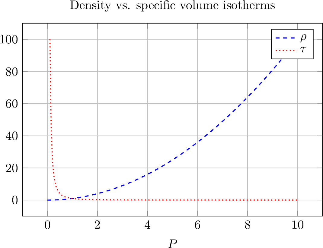
We also have that \(\partial_P \varrho = -\rho K_T < 0\). Furthermore, \(\require{physics} \partial_P^2 \varrho = -\partial_P(1 / c_T^2) = \frac{2}{c_T^3} \big(\pdv{c_T}{P}\big)_T\), where \(c_T^2 = 1 / (\rho K_T)\) is the isothermal sound speed. Hence, if \(c_T\) is an increasing function of \(P\) on each isotherm, then \(\varrho\) is a decreasing convex function of \(P\). For \(e(P,T)\), there is typically non-monotonic behavior in either of the variables, \(e(P,T)\) may be increasing or decreasing with respect to each variable. Therefore, we instead opt to solve a specific enthalpy equation for the temperature; that is, \[\label{eq:enthalpy95pte} \frakh(P,T) \eqq \sum_{m=1}^M e_m(P,T) + P \tau_m(P,T) - (e_0 + P \tau_0) = 0.\tag{16}\] Notice that \(\partial_T \frakh(P,T) = \partial_T h(P,T) = c_p > 0\).
4.1 Stopping criteria↩︎
Handling the convergence of the iterative methods requires a bit of care. The specific internal energy, like the pressure, can range across many different scales including negative values. The specific enthalpy, \(h\), also maintains this same behavior. We use the following relative error stopping criteria for the iterative methods, \[\begin{align} |\tau(P, T) - \tau_0| &< \epsilon \tau_0, \tag{17} \\ |e(P, T) - e_0| &< \epsilon (1 + |e_0|), \tag{18} \end{align}\] where \(\epsilon > 0\) is a unitless parameter typically around \(10^{-12}\). Since the specific internal energy can be identically zero, we incorporate a mix of relative and absolute error in the stopping criteria.
4.2 Single-Newton full-bisection method↩︎
Let \((P^{(0)}, T^{(0)}) \in \calP \times \Real_+\) be an initial guess, we first perform a full bisection method on the temperature to find the equilibrated temperature at the initial \(P^{(0)}\). That is, we find \(T^{(1)}\) which solves \(e(P^{(0)},T^{(1)}) - e_0 = 0\). We then apply one step of a standard Newton method to solve \(\varrho(P,T^{(1)}) = 0\) to find \(P^{(1)}\). This process is repeated until convergence is met. In general one could also employ other iterative solvers; e.g. bisection method. The specific algorithm for this method is provided in Algorithm 2.

4.3 2D Newton method↩︎
One of the more common numerical methods for solving a system of nonlinear equations is the 2D Newton method. The convergence can be very rapid; however, adaptation of the method is often required to improve its robustness. Let, \[\bsfE(P,T) \eqq \begin{pmatrix} \varrho(P,T) \\ e(P,T) - e_0 \end{pmatrix}\] then the Jacobian is, \[\require{physics} D\bsfE(P,T) \eqq \begin{bmatrix} \rho K_T & -\rho \beta \\ P\tau K_T - \beta \tau T & c_p - P \tau \beta \end{bmatrix} = \begin{bmatrix} \big(\pdv{\rho}{P}\big)_T & \big(\pdv{\rho}{T}\big)_P \\ \big(\pdv{e}{P}\big)_T & \big(\pdv{e}{T}\big)_P \end{bmatrix}.\] Then using 8 we find that \(\det(D\bsfE(P,T)) = \rho c_v K_T > 0\). The 2D Newton method is described by, \[\label{eq:2dnewton95pte95update} \begin{pmatrix} P^{(n+1)} \\ T^{(n+1)} \end{pmatrix} = \begin{pmatrix} P^{(n)} \\ T^{(n)} \end{pmatrix} - \frac{1}{\rho c_v K_T} \begin{bmatrix} c_p - P\tau \beta & \rho \beta \\ \tau (\beta T - P K_T) & \rho K_T \end{bmatrix} \bsfE(P^{(n)}, T^{(n)}).\tag{19}\] Note however, it is more computationally efficient to use the derivatives of \(\rho\) and \(e\) rather than the named thermodynamic derivatives: \(c_v\), \(c_p\), \(K_T\), and \(\beta\).
5 The cyclic method↩︎
While the 2D Newton method converges at a quadratic rate, it may fail to converge unless the initial guess is close enough to the root. Alternatively, the Newton-bisection method typically converges even when the initial guess is far away from the solution; however, the computational time is quite large. Solving PTE is just one part of solving the four-equation model, therefore the iterative solver should converge rapidly and accurately, since there could be billions of PTE solves at every time step.
There have been many proposed methods to resolve this issue, such as using a bisection method to find a safe starting point for the iterative method; see [54], or the trust region method (see [55] and [56]) which solves a safer subproblem (typically a minimization problem) to obtain the next iterate. We propose a novel, robust, and efficient method for solving nonlinear systems of equations from \(\Real^2\) to \(\Real^2\) that converges rapidly and is extremely robust to any arbitrary starting location. To the best of the author’s knowledge, such an algorithm has not appeared in the literature.
5.1 The general form↩︎
We first present the method in a generic form solving, \(\bF(\bx) = \ba\), where \(\bF : \Real^2 \to \Real^2\) is some nonlinear function and \(\ba = (a,b)^\sfT \in \Real^2\) is the initial datum. To be more explicit, we would like to solve the system: \[\begin{align} f(x,y) = a, \\ g(x,y) = b. \end{align}\] for \(f, g : \Real^2 \to \Real\), some nonlinear functions where \(\bF(\bx) \eqq (f(\bx), g(\bx))^\sfT\) and \(\bx = (x,y)\). The method we propose, takes advantage of the cyclic rule (also known as the triple product rule), see Corollary 1.
5.2 The cyclic method algorithm↩︎
We now describe the algorithm for the cyclic method. For a quick illustration of the procedure see Figure 3. We define the following 1-dimensional solution manifolds in the \((x,y)\)-plane: \[\begin{align} \frakF_a &\eqq \{ (x, y) : f(x,y) = a\}, \\ \frakG_b &\eqq \{ (x, y) : g(x,y) = b\}. \end{align}\] To simplify upcoming notation, we also define the lines in the \(x\)-\(y\) plane by, \[\require{physics} \begin{align} \sfI_\sfX^y(x_0, y_0) &\eqq \{(x,y) : y = y_0 + \Big(\pdv{y}{x}\Big)_\sfX(x_0, y_0)(x - x_0)\}, \\ \sfI_\sfX^x(x_0, y_0) &\eqq \{(x,y) : x = x_0 + \Big(\pdv{x}{y}\Big)_\sfX(x_0, y_0)(y - y_0)\}. \end{align}\] for \(\sfX\) some fixed quantity. A general outline of the method is now provided. Let \((x_0, y_0)\) be an initial guess, then:
Take a Newton step in the \(x\)-direction for \(f(x,y) = a\) from the point \((x_0, y_0)\) to find a point \((\tx_0, y_0)\).
Construct the tangent line, \(\sfI_f^x(\tx_0, y_0)\), to the curve \(\frakF_{f(\tx_0, y_0)}\) using the cyclic rule (Corollary 1).
Take a Newton step in the \(y\)-direction for \(g(x,y) = b\) from the point \((\tx_0, y_0)\) to find a point \((\tx_0, \ty_0)\).
Construct the tangent line, \(\sfI_g^y(\tx_0, \ty_0)\), to the curve \(\frakG_{g(\tx_0, \ty_0)}\) using the cyclic rule (Corollary 1).
Find the intersection point, \((x_1, y_1)\), of \(\sfI_f^x(\tx_0, y_0)\) and \(\sfI_g^y(\tx_0, \ty_0)\).
We now provide more explicit details on the construction of the tangent lines. After the first Newton step, we obtain the point \((\tx_0, y_0)\). The slopes of the tangent lines are provided by the cyclic rule, respectively as, \[\require{physics} \label{eq:cyclic95formula} \Big(\pdv{x}{y}\Big)_f(\tx_0, y_0) = - \frac{\big(\pdv{f}{y}\big)_x(\tx_0, y_0)}{\big(\pdv{f}{x}\big)_y(\tx_0, y_0)} \quad \text{ and } \quad \Big( \pdv{y}{x} \Big)_g(\tx_0, \ty_0) = -\frac{\big(\pdv{g}{x}\big)_y(\tx_0, \ty_0)}{\big(\pdv{g}{y}\big)_x(\tx_0, \ty_0)}.\tag{20}\] The intersection point of the two tangent lines, \(\sfI^x_f(\tx_0, y_0) \cap \sfI^y_g(\tx_0, \ty_0)\), is given by \[\require{physics} \tag{21} \begin{align} x_1 &\eqq \frac{ \tx_0 + \big( \pdv{x}{y} \big)_f(\tx_0, y_0) \big(\ty_0 - y_0 - \tx_0 \big( \pdv{y}{x} \big)_g(\tx_0, \ty_0) \big) }{ 1 - \big( \pdv{x}{y}\big)_f(\tx_0, y_0) \big( \pdv{y}{x} \big)_g(\tx_0, \ty_0) }, \tag{22} \\ y_1 &\eqq \ty_0 + \Big( \pdv{y}{x} \Big)_g(\tx_0, \ty_0) (x_1 - \tx_0). \end{align}\] If the denominator is zero, this implies that the two tangent lines are parallel, therefore, the application of this method should assess the existence of the intersection point. This process can be iterated until convergence and the concise description is provided in Algorithm 4.

This method can be generalized even more and tailored to the problem of interest. In particular, the derivatives in the \(x\)-\(y\) plane do not require \(f\) and \(g\) to be constant. We can instead choose some other quantity dependent on \(f\) and \(g\). For example, one could define mappings, \(p = p(f,g,x,y)\) and \(q = q(f,g,x,y)\), and apply standard calculus tecniques to derive \(\require{physics} \big(\pdv{x}{y}\big)_p\) and \(\require{physics} \big( \pdv{y}{x} \big)_q\) for use in the cyclic algorithm. This, allows us to avoid possible singularities in the derivatives and provide possible other improvements, such as convergence rates and robustness. This change in derivatives is used in the PTE application in Section 5.3.

5.3 Application of the cyclic method to PTE↩︎
We now proceed with the application of the method presented in Section 5.2 to the PTE system formulated by 15 and 16 . All calculations are the same as in Section 5.2 but with \((x,y)\) replaced with \((P,T)\), and \(f\) and \(g\) replaced with \(\varrho\) and \(\frakh\). However, instead of using \(\require{physics} \big( \pdv{T}{P} \big)_h\) we instead use \(\require{physics} \big( \pdv{T}{P} \big)_s\) and switch back to \(\require{physics} \big( \pdv{T}{P} \big)_h\) if the line intersection step lands out of bounds. In our numerical tests, we found this to be the most robust and efficient.
For reference we have the following thermodynamic identities from the cyclic rule: \[\require{physics} \begin{align} \Big( \pdv{P}{T} \Big)_\rho &= -\frac{\big(\pdv{\rho}{T}\big)_P}{\big(\pdv{\rho}{P}\big)_T} = \frac{\beta}{K_T}, \tag{23} \\ \Big( \pdv{T}{P} \Big)_s &= -\frac{\big(\pdv{s}{P}\big)_T}{ \big( \pdv{s}{T} \big)_P} = \frac{\beta T \tau}{c_p}, \tag{24} \\ \Big( \pdv{T}{P} \Big)_h &= -\frac{\big(\pdv{h}{P}\big)_T}{\big(\pdv{h}{T}\big)_P} = \frac{\beta T \tau - \tau}{c_p}. \tag{25} \end{align}\] Note, each of these derivatives are finite real valued numbers since \(c_p > 0\) and \(K_T > 0\). The specific algorithm is described in Algorithm 5 and is always well-posed under thermodynamic stability as proven in Theorem 5.

Theorem 5 (Non-parallel tangent lines). Assuming thermodynamic stability (Definition [def:thermo95stability]), Algorithm 5 is well-posed in the sense that the tangent lines in the \(P\)-\(T\) space are not parallel. More specifically, either \(\sfI_\rho^P(P_0, T_0) \cap \sfI_s^T(P_1, T_1) \neq \emptyset\) or \(\sfI_\rho^P(P_0, T_0) \cap \sfI_h^T(P_1, T_1) \neq \emptyset\), for all \((P_0, T_0), (P_1, T_1) \in \sfR\).
Proof. Notice that \(\require{physics} \big( \pdv{T}{P} \big)_s > \big( \pdv{T}{P} \big)_h\) for all \(\tau > 0\) from 24 and 25 . Therefore, the sets: \(\sfI_\rho^P(P_0, T_0) \cap \sfI_s^T(P_1, T_1)\) or \(\sfI_\rho^P(P_0, T_0) \cap \sfI_h^T(P_1, T_1)\), cannot both be empty. ◻
6 Equation of state↩︎
We describe several equations of state which will be used in the testing of the PTE solver. We provide only the necessary details in order to perform the PTE solve.
6.1 Ideal and stiffened gas↩︎
The ideal and stiffened gas laws are provided by, \[\begin{align} \rho_{\text{ideal}}(P,T) = \frac{P}{RT}, \quad &\text{ and } \quad e_{\text{ideal}}(P,T) = c_v T \\ \rho_{\text{stiff}}(P,T) = \frac{P+P_\infty}{RT}, \quad &\text{ and } \quad e_{\text{stiff}}(P,T) = \frac{c_v T (P + \gamma P_\infty)}{P + P_\infty} + q \end{align}\] where \(P_\infty > 0\), \(q \in \Real\), \(\gamma = c_p / c_v\) and \(R = c_p - c_v\) for \(c_p > c_v > 0\). The parameters we use for ideal and stiffened gas are provided in Table 1.
| \(c_p\) \((\SI{}{\kilo\joule\per\gram\per\kelvin})\) | \(c_v\) \((\SI{}{\kilo\joule\per\gram\per\kelvin})\) | \(P_\infty\) \((\SI{}{\giga\pascal})\) | \(q\) \((\SI{}{\kilo\joule\per\gram})\) | |
|---|---|---|---|---|
| Ideal gas | 0.0014 | 0.001 | - | - |
| Stiffened gas | 0.0085 | 0.0012 | 0.01 | 0 |
6.2 Reactant and product Davis EOS↩︎
PTE is often assumed among products and reactants in the context of high explosives detonation due to it’s relative simplicity and guarantee of thermodynamic consistency, despite the PTE assumption not being generally accurate on the detonation timescale. This is discussed in [12] and references therein. This motivates testing with equations of state used in HE products and reactants. In particular, we shall use the reactant Davis and product Davis equations of state. We follow the descriptions provided in [57] and use the parameters from [58].
The reactant Davis pressure and specific internal energy are given by, \[\begin{align} e(\tau, T) &= e_s(\tau) + \frac{c_v^0 T_s(\tau)}{1 + \alpha_{ST}} \Big[ \Big( \frac{T}{T_s(\tau)} \Big)^{1 + \alpha_{ST}} - 1 \Big], \\ P(\tau, T) &= P_s(\tau) + \frac{\Gamma(\tau)}{\tau} \frac{c_v^0 T_s(\tau)}{1 + \alpha_{ST}} \Big[ \Big( \frac{T}{T_s(\tau)} \Big)^{1 + \alpha_{ST}} - 1 \Big] \end{align}\] where \[\begin{align} T_s(\tau) &= T_0 \begin{cases} \big( \frac{\tau}{\tau_0} \big)^{-\Gamma_0}, &\quad \text{ if } \tau > \tau_0, \\ \big( \frac{\tau}{\tau_0} \big)^{-(\Gamma_0 + Z)} \exp\big(-Z \big(1 - \frac{\tau}{\tau_0} \big) \big), &\quad \text{ if } \tau \leq \tau_0, \end{cases} \\ e_s(\tau) &= e_0 + \frac{A^2}{16B^2} \begin{cases} \exp(4By) - 4By - 1, &\, \text{ if } \tau > \tau_0, \\ \sum_{n=2}^4 \frac{(4By)^n}{n!} + C \frac{(4By)^5}{5!} + \frac{4By^3}{3(1 - y)^3}, &\, \text{ if } \tau \leq \tau_0, \end{cases} \tag{26} \\ P_s(\tau) &= \frac{A^2}{4B\tau_0} \begin{cases} \exp(4By) - 1, &\, \text{ if } \tau > \tau_0, \\ \sum_{n=1}^3 \frac{(4By)^n}{n!} + C \frac{(4By)^4}{4!} + \frac{y^2}{(1 - y)^4}, &\, \text{ if } \tau \leq \tau_0, \end{cases} \tag{27} \\ \Gamma(\tau) &= \begin{cases} \Gamma_0, &\, \text{ if } \tau > \tau_0, \\ \Gamma_0 + Zy, &\, \text{ if } \tau \leq \tau_0, \end{cases} \tag{28} \end{align}\] with \(y \eqq 1 - \frac{\tau}{\tau_0}\).
The product Davis EOS is provided by, \[\begin{align} P(\tau, e) &= (\gamma - 1 + F(\tau)) \frac{e}{\tau} - \frac{bF(\tau)}{\tau} (e - e_s(\tau)), \\ F(\tau) &= \frac{2a}{\big( \frac{\tau}{\tau_c} \big)^{2n} + 1}, \\ e_s(\tau) &= e_c \Big( \frac{\tau}{\tau_c} \Big)^{-(\gamma-1+2a)} \Big( \frac{1}{2} \Big( \frac{\tau}{\tau_c} \Big)^{2n} + \frac{1}{2} \Big)^{a/n}, \end{align}\] where \(\gamma > 1\) and \(\tau_c, a, b, n > 0\) are some parameters for modeling the products. For the thermal part we have, \[\begin{align} e(\tau, T) &= c_v (T - T_s(\tau)) + e_s(\tau), \\ T_s(\tau) &= T_c \Big( \frac{\tau}{\tau_c} \Big)^{-(\gamma-1+2a(1-b))} \Big( \frac{1}{2} \Big( \frac{\tau}{\tau_c} \Big)^{2n} + \frac{1}{2} \Big)^{a(1-b)/n}, \end{align}\] where \(c_v > 0\) is a constant specific heat capacity (at constant volume) and \(T_c > 0\). For both the reactant and product Davis EOS, we compute the density by solving the nonlinear equation \(P(\tau, e(\tau,T_j)) = P_i\) for \(\tau_{ij}\). Then the energy is computed by \(e_{ij} \eqq e(v_{ij}, T_j)\).
6.3 Simple MACAW↩︎
Lastly, we use the Simple MACAW EOS found in [59] with the parameters for copper described in [59]. This EOS is a simplified equation of state of the one presented in [60]. We omit the details as they are presented concisely in [59].
7 Numerical results↩︎
We deploy a series of tests to determine the efficiency and accuracy of the methods for a variety of different EOS.
7.1 Preliminaries↩︎
We will often be comparing the number of “steps” that the numerical method has taken. Since each method is fairly distinct, we would like to clarify the definition of a “step” for each method.
A step for the cyclic method consists of the two one-dimensional Newton steps with tangent line intersection. A step for the Newton-bisection method consists of the full bisection algorithm in temperature with the single one-dimensional Newton step. Lastly, a step for the 2D Newton method is simply the one update provided by 19 . All EOS are approximated with 350 grid points in the pressure and temperature partitions and are distributed logarithmically; see Section 3.2.
7.2 Random data trials↩︎
In order to demonstrate the robustness and efficiency of the new method, we generate random initial data \((P_0, T_0, \bY_0) \in \sfR \times \Delta\) and compute \(e_0\) and \(v_0\) from \((P_0, T_0, \bY_0)\). Then we generate a random initial guess \((P_\text{guess}, T_\text{guess}) \in \sfR\). All random data is generated using the
standard C++ library implementation of the 19937 Mersenne Twister (see [61]), std::mt19937, with a logarithmic
distribution. We fix the max number of iterations to be 100 for each method. If an iterative method exceeds this threshold then the test is flagged as a failure. All tests were run with 10,000 trials each.
7.2.1 Test 1↩︎
For the first test, we use the ideal gas and stiffened gas EOS. The pressure-temperature domain is \(\sfR = [\SI{e-8}{\giga\pascal}, \SI{10}{\giga\pascal}] \times [\SI{0.01}{\kelvin}, \SI{2e4}{\kelvin}]\). The statistics are reported in Table 2. We note that on average, the cyclic method is approximately 2 times faster than the 2D Newton and more than 5 times faster than the Newton-bisection method.
| Random trial #1 (Ideal/Stiffened) | |||
|---|---|---|---|
| Cyclic | 2D Newton | Newton+Bisection | |
| Failure rate | 0% | 61.6% | 0% |
| Average steps | 6.7 | 41.7 | 7.6 |
| Average bisections | - | - | 308 |
| Average CPU time | 2.8 × 10⁻⁴ s | 5.2 × 10⁻⁴ s | 1.5 × 10⁻³ s |
7.2.2 Test 2↩︎
For the second test, we use the ideal gas , stiffened-gas, and the simple MACAW on the domain \(\sfR = [\SI{e-12}{\giga\pascal}, \SI{e3}{\giga\pascal}] \times [\SI{e-3}{\kelvin}, \SI{e5}{\kelvin}]\). The statistics are reported in Table 3. The cyclic method is approximately 2.8 times faster than the 2D Newton method, and almost 6 times faster than the Newton-bisection method.
| Random trial #2 (Ideal/Stiffened/Simple MACAW) | |||
|---|---|---|---|
| Cyclic | 2D Newton | Newton+Bisection | |
| Failure rate | 0% | 94.3% | 0.75% |
| Average steps | 7.2 | 58.9 | 7.9 |
| Average bisections | - | - | 362 |
| Average CPU time | 3.9 × 10⁻⁴ s | 1.1 × 10⁻³ s | 2.3 × 10⁻³ s |
7.2.3 Test 3↩︎
We now consider a much more challenging test (for all methods) and discuss some of the issues. We consider a mixture of five materials: simple MACAW, product Davis, reactant Davis, stiffened gas, and ideal gas. The \(P\)-\(T\) domain is given by \(\sfR = [\SI{e-8}{\giga\pascal}, \SI{e3}{\giga\pascal}] \times [\SI{e-3}{\kelvin}, \SI{5e4}{\kelvin}]\). The statistics are presented in Table 4.
We have omitted the statistics for the 2D Newton method due to the very high failure rate. Unfortunately the failure rate for the cyclic method is much higher than the Newton-bisection method. From analyzing some of the problems which failed, we found that the cyclic method could fail by “ping-ponging” between two points or “sailing” around the solution, unable to get within the convergence tolerance. We believe that the tabular approximation is partly the source of these problems as refining the tables can decrease the failure rate. We also slightly modify this test to investigate the causes of the failure in Sections 7.2.4 and 7.2.5.
| Random trial #3 (Five material) | |||
|---|---|---|---|
| Cyclic | 2D Newton | Newton+Bisection | |
| Failure rate | 47.8% | 99.9% | 7.8% |
| Average steps | 24.7 | - | 76 |
| Average bisections | - | - | 4013 |
| Average CPU time | 1.8 × 10⁻³ s | - | 4.1 × 10⁻² s |
7.2.4 Test 4↩︎
We repeat the same test in Section 7.2.3 except we change \(T_{\max}\) from \(\SI{5e4}{\kelvin}\) to \(\SI{5e3}{\kelvin}\). The results are reported in Table 5. We now see that the failure rate has drastically decreased for the cyclic method and increased for the Newton-bisection method. The cyclic method is also almost 19 times faster than the Newton-bisection method. Again, we omit the statistics for the 2D Newton method due to the high failure rate.
| Random trial #4 (Five material) | |||
|---|---|---|---|
| Cyclic | 2D Newton | Newton+Bisection | |
| Failure rate | 5.2% | 98.4% | 25.2% |
| Average steps | 9.8 | - | 27.6 |
| Average bisections | - | - | 5287 |
| Average CPU time | 8.0 × 10⁻⁴ s | - | 1.5 × 10⁻² s |
7.2.5 Test 5↩︎
For the last test, we simply repeat the test in Section 7.2.3 except we now omit the reactant Davis EOS. The results are reported in Table 6. Again, it seems that a lot of the difficulty stems from the reactant Davis EOS. This is discussed in Remark [rem:path95react95davis]
| Random trial #5 (Four material) | |||
|---|---|---|---|
| Cyclic | 2D Newton | Newton+Bisection | |
| Failure rate | 0% | 86% | 3.2% |
| Average steps | 7.1 | 63 | 8.2 |
| Average bisections | - | - | 606 |
| Average CPU time | 5.0 × 10⁻⁴ s | 1.5 × 10⁻³ s | 3.2 × 10⁻³ s |
In the numerical illustrations we have provided below, we have found that the cyclic method is sensitive to the tabular approximation of the reactant Davis. That is, the refinement of the tabular approximation of the reactant Davis may dictate convergence or divergence. Simply decreasing the size of the \(P\)-\(T\) domain can cause the cyclic method to switch from divergence to convergence. This also applies to convergence of the other methods as well. Furthermore, without a careful selection of the pressure partition, \(\sfP\), one may find that the numeric \([\rho^{i,j}_m \rho^{i+1,j}_m] = 0\) at high temperature and low pressures, despite the analytic reactant Davis EOS having positive isothermal bulk modulus. We have chosen appropriate refinement levels when using the reactant Davis EOS in order to avoid this issue.
7.3 Two-state transition↩︎
Often when solving the four-equation model, one uses the pressure and temperature solution of the previous time step. Since solving the four-equation model is out of scope for this paper, we construct a series of data that mimics a transition between two materials and use the previous solution as a guess for the next data. We use an \(\arctan\) function to interpolate between the data points given by: \[\label{eq:contact95func} C(x; y_0, y_1) = \frac{1}{2} (y_0 + y_1) + \frac{1}{2} (y_1 - y_0) \frac{\arctan(kx)}{\arctan(k)},\tag{29}\] where \(y_L\) and \(y_R\) are the left and right thermodynamic states and \(k = 100\) is a parameter used increase the sharpness of the transition. For all problems, we select \((P_Z, T_Z) \in \sfR\) then the datum are computed by \(\tau_Z = \tau(P_Z, T_Z, \bY_Z)\) and \(e_Z = e(P_Z, T_Z, \bY_Z)\) for \(Z \in \{L,R\}\). The transitional data functions are described by \(C(x; \tau_L, \tau_R)\), \(C(x; e_L, e_R)\), \(C(x; Y_{0,L}, Y_{0,R})\), and \(Y_1(x) = 1 - C(x; Y_{0,L}, Y_{0,R})\) for all \(x \in (-1, 1)\). The sampling domain is \(D = [-1,1]\). Setting \(N = 200\), the sample points are given by \(x_i = -1 + \frac{2i}{N+1}\) for \(i \in \intset{1}{N}\). Plots of the transitional data are provided in Figures 6 and 7. For all tests in this section, we use \(\sfR = [\SI{e-8}{\giga\pascal}, \SI{100}{\giga\pascal}] \times [\SI{0.001}{\kelvin}, \SI{5e4}{\kelvin}]\).


7.3.1 Two-state: Stiffened & ideal gas contact↩︎
For the first test, try a contact between ideal and stiffened gas laws; that is, the pressures are equal on both sides. The specific data we use is: \[\begin{align} (P_L, T_L, \bY_L) &= (\SI{1.01e-4}{\giga\pascal}, \SI{1000}{\kelvin}, (1,0)), \\ (P_R, T_R, \bY_R) &= (\SI{1.01e-4}{\giga\pascal}, \SI{300}{\kelvin}, (0,1)), \end{align}\] where the left state is the stiffened gas law and the right state is the ideal gas law. This smooth mixture transition approximating the contact is similar to what may appear from numerical viscosity in a first order method when solving the four-equation model. In this case, we see the PTE solutions plotted in Figure 8 throughout the transition. The statistics are reported in Table 7.
| Stiffened gas/Ideal gas contact | |||
|---|---|---|---|
| Cyclic | 2D Newton | Newton+Bisection | |
| Failure rate | 0% | 50% | 0% |
| Average steps | 2.7 | 16.4 | 24.4 |
| Average bisections | - | - | 1103 |
| Average CPU time | 1.6 × 10⁻⁴ s | 2.2 × 10⁻⁴ s | 5.2 × 10⁻³ s |
7.3.2 Two-state: Simple MACAW & ideal gas↩︎
For the first test, use the Simple MACAW for the left state and ideal gas for the right state. The left and right data are provided by, \[\begin{align} (P_L, T_L, \bY_L) &= (\SI{1.01e-4}{\giga\pascal}, \SI{300}{\kelvin}, (1,0)), \\ (P_R, T_R, \bY_R) &= (\SI{1}{\giga\pascal}, \SI{1500}{\kelvin}, (0,1)). \end{align}\] A plot of the PTE solution along the transition is provided in Figure 8 and the statistics in Table 8. In this problem, the 2D Newton is able to converge 100% of the time when using the previous solution as the initial guess. But as in Section 7.3.1 and Section 7.3.3, this is not sufficient.
| Simple MACAW/Ideal gas transition | |||
|---|---|---|---|
| Cyclic | 2D Newton | Newton+Bisection | |
| Failure rate | 0% | 0% | 0% |
| Average steps | 2.4 | 13.6 | 3.8 |
| Average bisections | - | - | 159 |
| Average CPU time | 1.3 × 10⁻⁴ s | 1.8 × 10⁻⁴ s | 7.9 × 10⁻⁴ s |
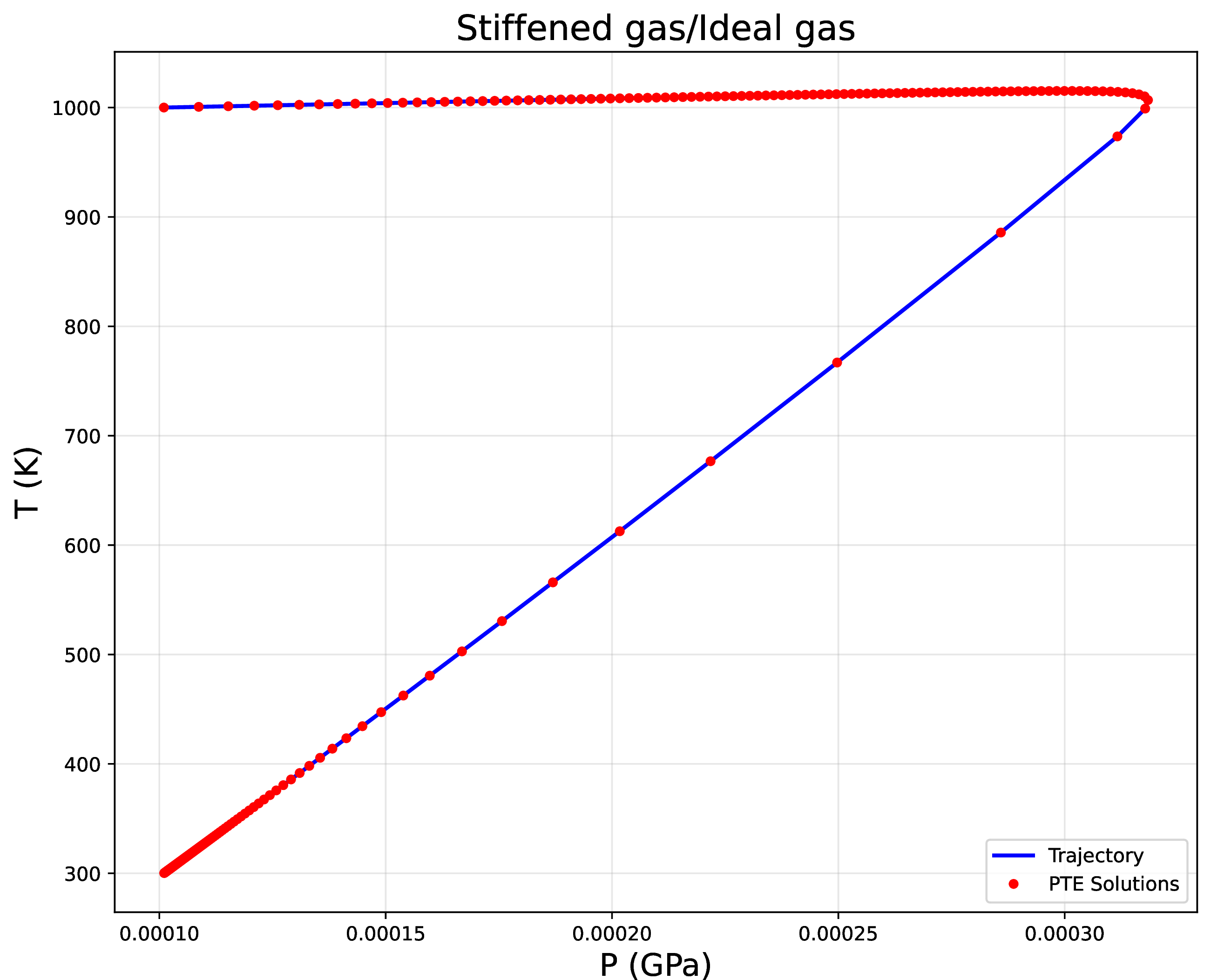
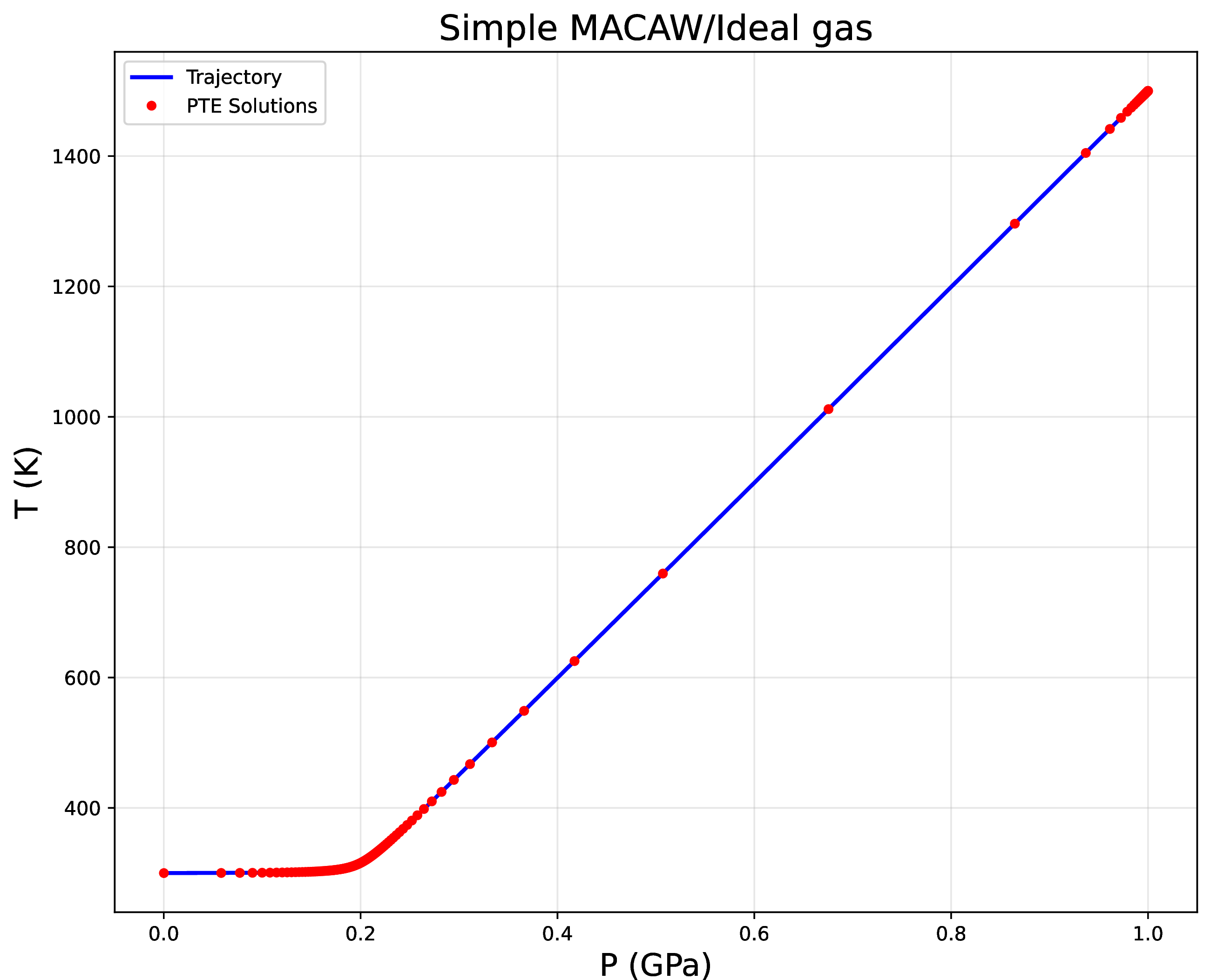
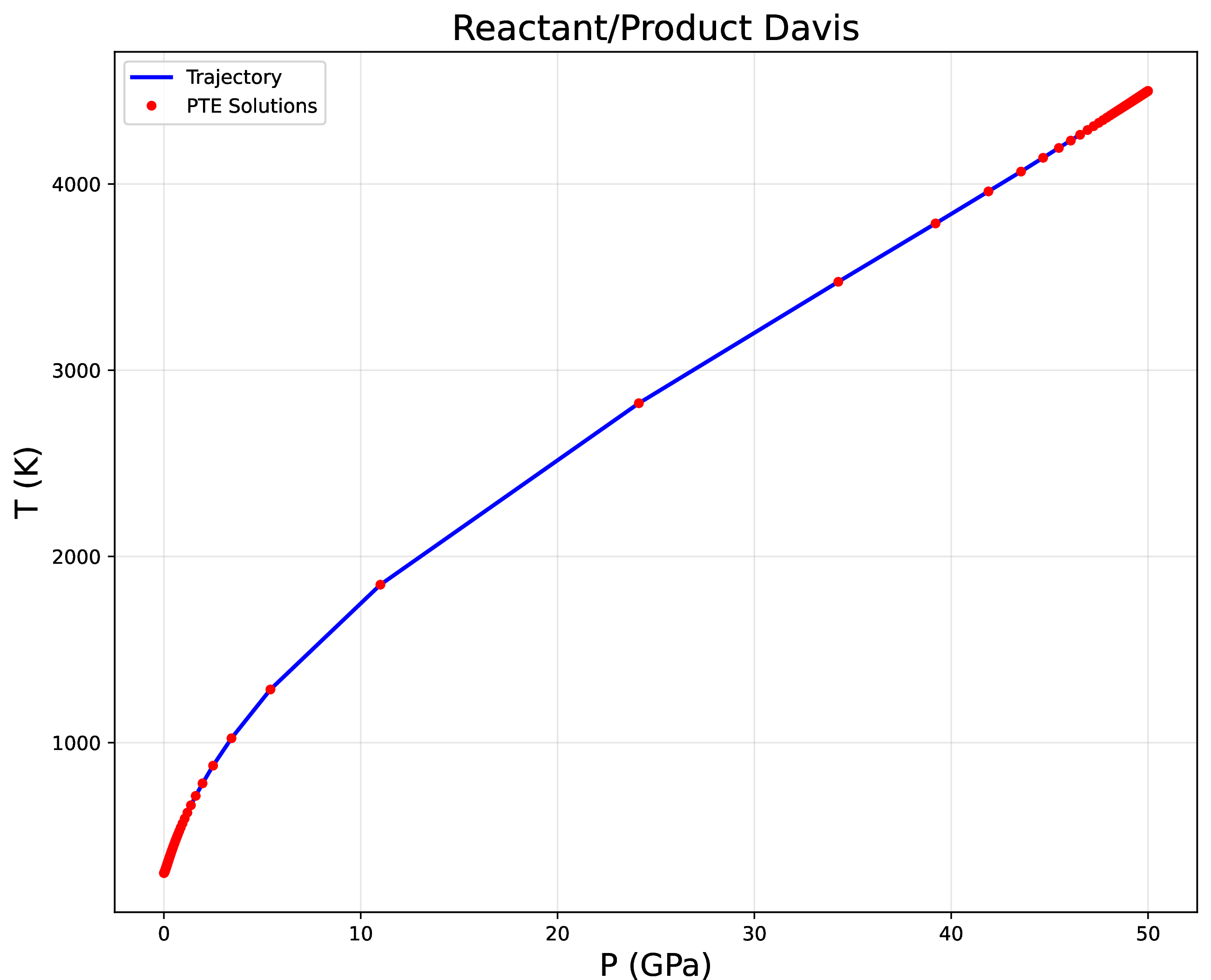
Figure 8: The PTE solutions for the problems in Section 7.3.1 (top left), Section 7.3.2 (top right), and Section 7.3.3 (bottom)..
7.3.3 Two-state: Product & reactant Davis↩︎
For the next test we consider a transition between Davis reactants to Davis products. The left and right data are: \[\begin{align} (P_L, T_L, \bY_L) &= (\SI{1.01e-4}{\giga\pascal}, \SI{300}{\kelvin}, (1,0)), \\ (P_R, T_R, \bY_R) &= (\SI{50}{\giga\pascal}, \SI{4500}{\kelvin}, (0,1)). \end{align}\] The statistics are reported in Table 9 and the plot of the PTE solutions are provided in Figure 8. Note in Figure 8, the PTE solutions can be quite far apart, in which case, the solution at a previous state may not be sufficiently close for iterative methods to converge.
| Reactant/product Davis transition | |||
|---|---|---|---|
| Cyclic | 2D Newton | Newton+Bisection | |
| Failure rate | 0% | 51% | 3% |
| Average steps | 3.8 | 13.8 | 8.9 |
| Average bisections | - | - | 503 |
| Average CPU time | 1.8 × 10⁻⁴ s | 1.9 × 10⁻⁴ s | 1.9 × 10⁻³ s |
7.4 Grid test↩︎
We now demonstrate the robustness of the nonlinear solves with a “grid test”. We start with the true pressure temperature solution, \((P_0, T_0)\), as well as the mass fractions, \(\bY_0\), then compute the corresponding data: \(\tau_0 = \tau(P_0, T_0, \bY_0)\) and \(e_0 = e(P_0, T_0, \bY_0)\). We then run the numerical method for every midpoint of every cell pressure-temperature cell, \(\sfR^i_j\), in our \(P\)-\(T\) domain and count the number of iterations it took for convergence to be achieved. If the method exceeds 100 steps then we flag it as a failure. For the Newton-bisection method we include the total number of bisection steps in addition to the Newton steps for the respective plots.
7.4.1 Test 1↩︎
We use the simple MACAW (\(Y_0 = 0.95\)) and the product Davis (\(Y_1 = 0.05\)); the true solution is \(P_0 = \SI{31}{\giga\pascal}\) and \(T_0 = \SI{2000}{\kelvin}\). The pressure-temperature domain is \(\sfR = [\SI{e-8}{\giga\pascal}, \SI{100}{\giga\pascal}] \times [\SI{0.001}{\kelvin}, \SI{5e4}{\kelvin}]\). Plots of the iteration counts are shown in Figure 9. Note the “striping” effect of the Newton-bisection method; this is reproduced in all test problems as the method essentially reduces the 2D problem to a 1D problem.
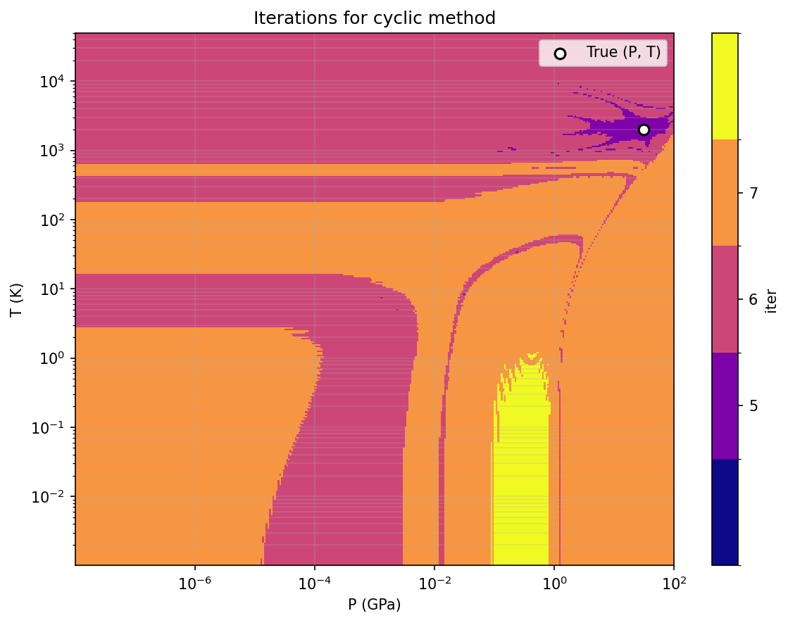
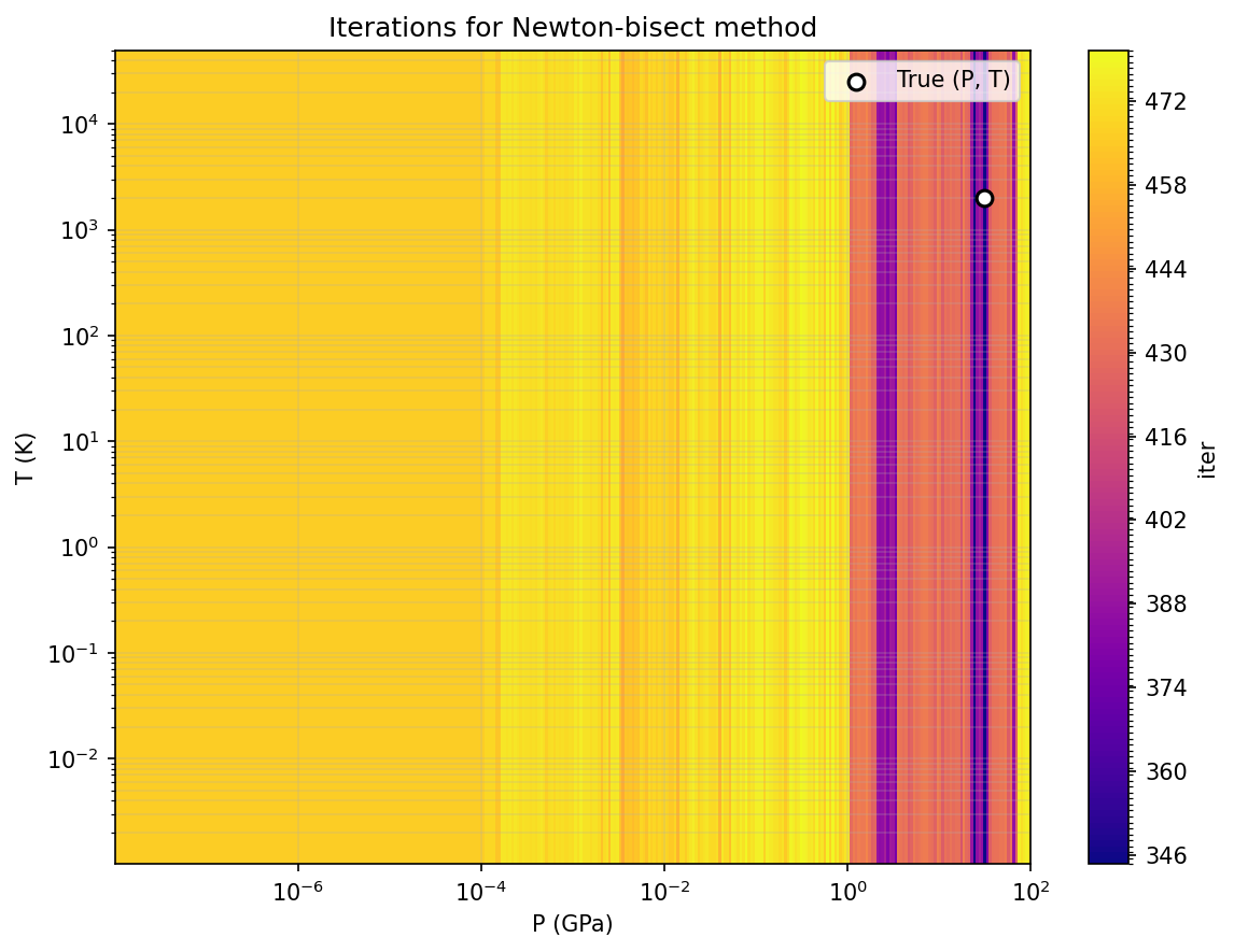
Figure 9: Plots of the number of iterations for each starting point for the simple MACAW + product Davis test. Results for the 2D Newton method omitted due to the very high failure rate..
7.4.2 Test 2↩︎
We now consider a test case with the reactant Davis EOS (\(Y_0 = 0.05\)) and product Davis EOS (\(Y_1 = 0.95\)). The true pressure and temperature are \(P_0 = \SI{39}{\giga\pascal}\) and \(T_0 = \SI{4100}{\kelvin}\). As in the previous section, we use the same domain, \(\sfR = [\SI{e-8}{\giga\pascal}, \SI{100}{\giga\pascal}] \times [\SI{0.001}{\kelvin}, \SI{5e4}{\kelvin}]\). The iteration plots are presented in Figure 10.
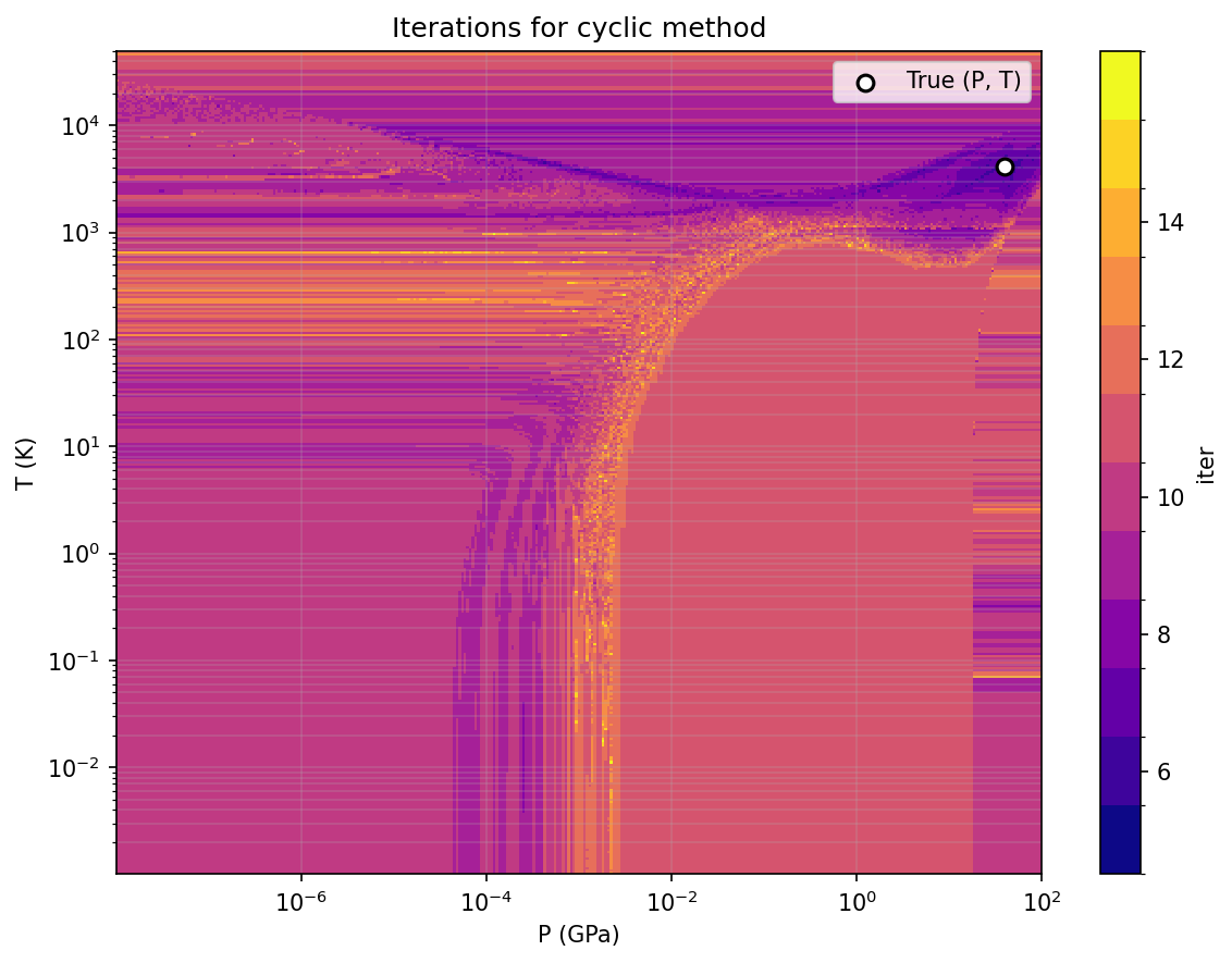

Figure 10: Iteration plots for reactant and product Davis EOS problem in Section 7.4.2. Results for 2D Newton method omitted due to high failure rate..
7.4.3 Test 3↩︎
Next we run a test using ideal gas, stiffened gas, simple MACAW, reactant Davis, and product Davis with \(Y_m = 0.2\) for each \(m \in \intset{1}{5}\). Again using the same pressure-temperature domain as in the previous tests. The true solution is chosen to be \(P_0 = \SI{3e-3}{\giga\pascal}\) and \(T_0 = \SI{800}{\kelvin}\). Results are presented in Figure 11.
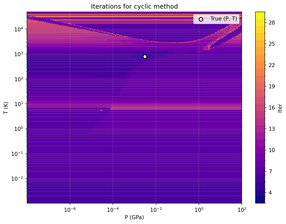
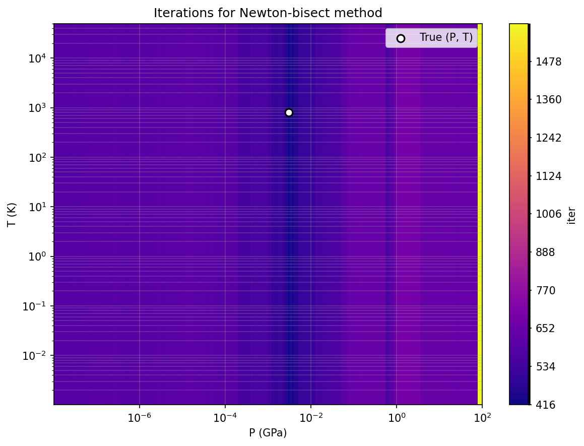
Figure 11: Iteration plots for five material problem in Section 7.4.3. Results for 2D Newton method omitted due to high failure rate..
7.4.4 Test 4↩︎
Next we run a test using ideal gas (\(Y_1 = 0.2\)), stiffened gas (\(Y_2 = 0.3\)) and the simple MACAW (\(Y_3 = 0.5\)). Again using the same pressure-temperature domain as in the previous tests. The true solution is chosen to be \(P_0 = \SI{3e-5}{\giga\pascal}\) and \(T_0 = \SI{250}{\kelvin}\). Results are presented in Figure 12. Noting here that the 2D Newton method does have some large regions where it is able to converge, compares to the previous tests.
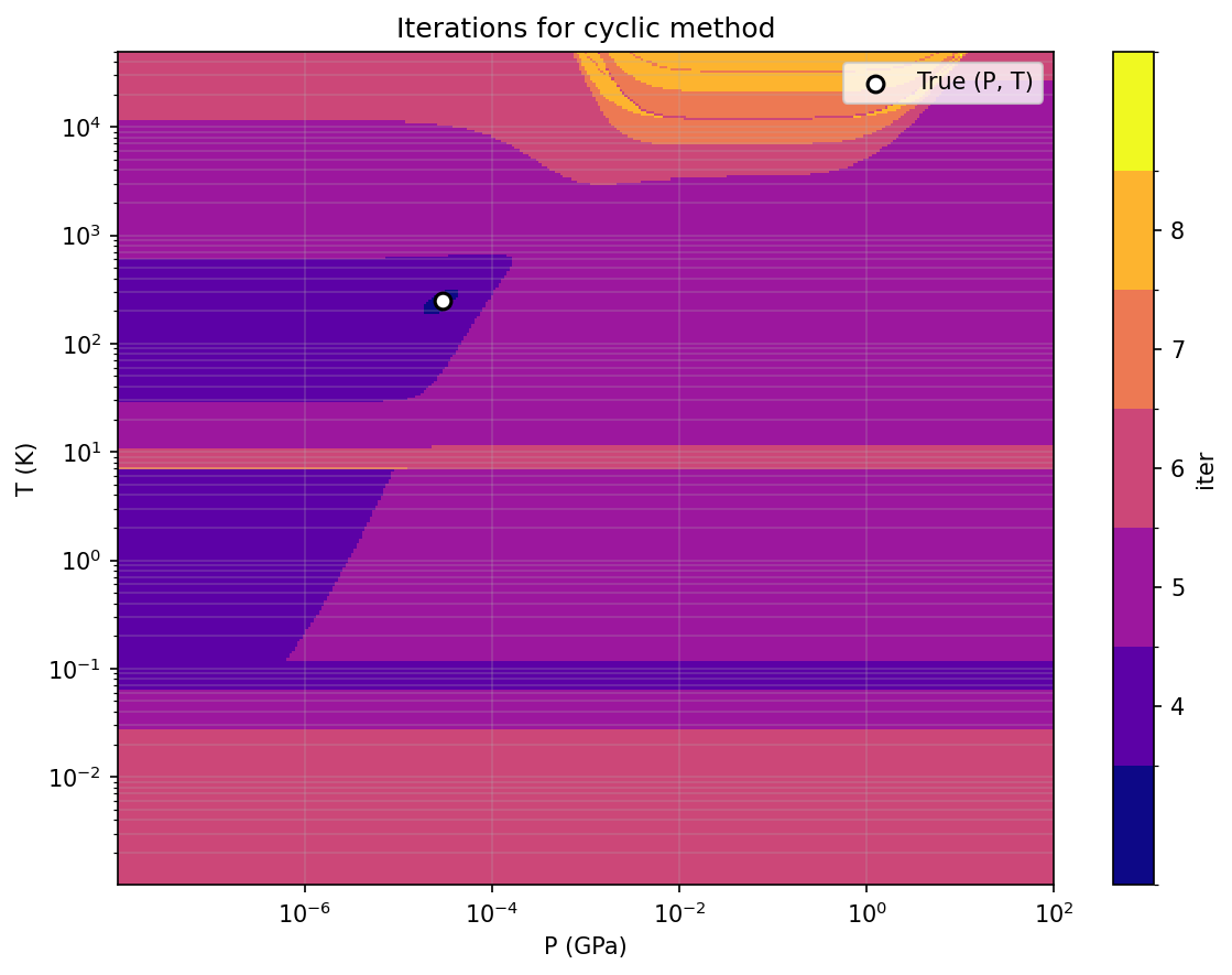
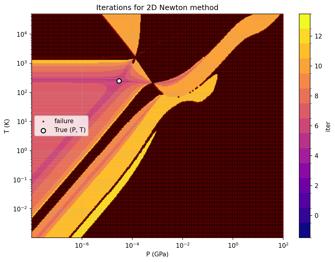
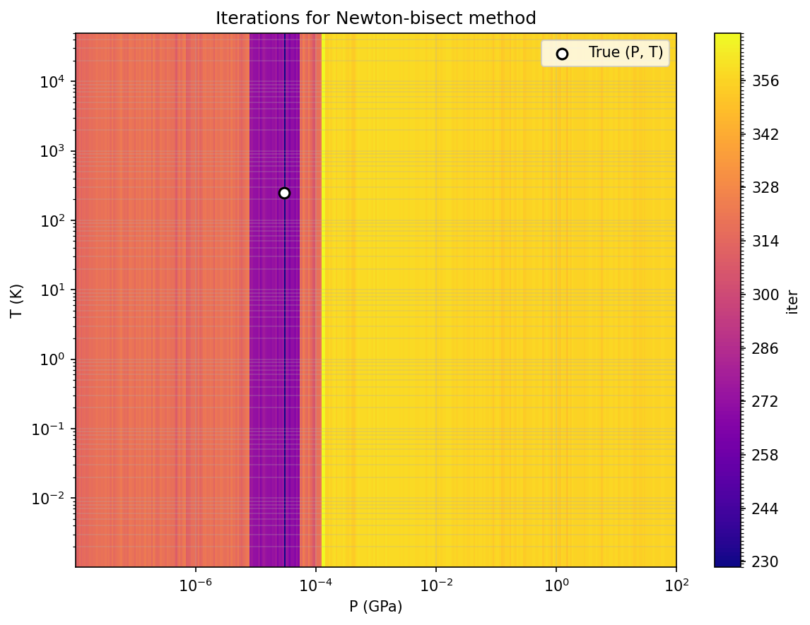
Figure 12: Iteration plots for three material problem (ideal, stiffened gas, simple MACAW) in Section 7.4.4..
8 Conclusion↩︎
We have analyzed the pressure-temperature equilibrium closure model imposed on the four-equation model for general equations of state that are thermodynamically stable. We covered the mixture thermodynamic derivatives and various other thermodynamic properties. In particular, the admissible set was identified in Definition 5 and was found to be a convex set owing to Theorem 4. Assuming the state vector belongs to the admissible set, the existence and uniqueness of solutions to the PTE system was proven in Theorem 3. We then introduced a possible method for constructing a tabular approximation of an equation of state in Section 3 in order to avoid expensive solves for \(\rho(P,T)\). A transformation of the PTE system is provided which aides the nonlinear solvers. Then a novel nonlinear solver was introduced, the cyclic method, which was applied to the PTE system; demonstrating its robustness and computational efficiency.
Acknowledgments↩︎
The authors thank their colleagues from Los Alamos National Laboratory: Tariq Aslam, Eduardo Lozano, and Jeffery Peterson for their insightful discussions on thermodynamics and equations of state.
References↩︎
Draft version, 2026-06-29↩︎