1 Introduction↩︎

This paper studies a family of metrics between real-variable functions, exploring their stability to geometric deformations and additive noise. The definitions of these metrics makes use of a function’s “scale-space” representation, in which the function is convolved with a sequence of Gaussian kernels of varying widths. Each function is thereby replaced by a stack of functions, of varying resolution. The distance \(\mathrm{D}_{\alpha,p,r}(f,g)\) between two functions \(f\) and \(g\) in \(L^r \cap L^1\) is then defined as a weighted sum of the distances across each stack; the precise definition is given in Section 2.

Such metrics, and the ideas underlying their construction, have previously appeared in numerous works:

In the harmonic analysis literature, the norms that induce these metrics are equivalent to the dual norms of Besov spaces (certain classes of smooth functions) [1], [2].
Classical imaging processing techniques make use of an image’s scale-space representation via Gaussian smoothing [3]. For instance, features extracted from the scale-space representation of a function are used in the well-known SIFT algorithm for feature detection [4], [5].
The special case where \(p=r=1\) and \(0 < \alpha < 1\) is known to be metrically equivalent to the Wasserstein distance with ground distance \(|x-y|^{\alpha}\); see [6], as well as the related works [7], [8], which employ multiscale analysis via wavelets rather than Gaussians.
Analogous metrics over more abstract spaces that exhibit a multiscale structure (such as spaces endowed with hierarchical tree metrics) have been studied in data science applications; for instance, see [6], [9]–[14].

In the present work, we explore the stability of these metrics \(\mathrm{D}_{\alpha,p,r}\) to distortions of their inputs, both under measure-preserving geometric deformations and additive noise. We focus specifically on applications to image-processing (i.e.to functions on \(\mathbb{R}^2\), and their discretizations), though many of our results may be generalized to other dimensions. One of the scientific motivations for our work is the robust comparison of 2D tomographic projections of 3D functions, a setting which occurs in applications like cryo-electron microscopy (cryo-EM) [15]–[19]. Various metrics related to Wasserstein distances have been proposed for image comparison in cryo-EM recently [20], [21], not to mention scores of other applications and theoretical results [7], [22]–[29]. Because the metrics \(\mathrm{D}_{\alpha,p,r}\) generalize a metric equivalent to Wasserstein, it is natural to explore their properties as well.

Because the images in cryo-EM typically undergo random in-plane rotations, it is important to define a rotation-invariant version of the metric \(\mathrm{D}_{\alpha,p,r}\), which minimizes the distance between the input functions over all in-plane rotations, as is done in [20] and [21]. As will become clear later, for this to be computationally feasible we restrict \(r=2\); see Section 5.2 for details.

The main contributions of the paper are as follows:

We bound the distortion between \(\mathrm{D}_{\alpha,p,r}(f,g)\) when \(g\) is a perturbation of \(f\), in terms of the maximum displacement of the perturbation. (In fact, the bound extends to the more general setting where \(f\) and \(g\) are projections of functions that are perturbations of each other.)
If \(f\) and \(g\) are 2D projections of a fixed 3D function, we prove robustness of the rotationally-invariant metric \(\mathrm{D}_{\alpha,p,r}(f ,g; \,\mathrm{SO}(2))\) to changes in the projection angle.
When \(r=2\), we define a fast algorithm for calculating both \(\mathrm{D}_{\alpha,p}(f,g)\) and the rotationally-invariant metric \(\mathrm{D}_{\alpha,p}(f,g;\, \mathrm{SO}(2))\). For functions discretized on an \(n\)-by-\(n\) Cartesian grid, the cost of these algorithms scale like \(O(n^2 \log(n))\).
We prove robustness of the discretization to additive sub-Gaussian noise.
Finally, we report on numerical experiments illustrating the aforementioned results.

2 The scale-space metrics↩︎

The metrics will be defined by several user-set parameters: \(\tau_0 > 0\), \(0 < \omega < 1\), \(r \ge 1\), \(p \ge 1\), and \(\alpha > 0\). Typically, we will take \(\omega = 1/2\); and when rotational-invariance is needed, \(r=2\).

For a value \(\tau > 0\), denote by \(G_\tau\) the Gaussian kernel at scale \(\tau\), defined by \[\begin{align} G_\tau(x) = \frac{1}{(\pi \tau)^{d/2}} e^{-|x|^2 / \tau}. \end{align}\] For fixed values \(\tau_0 > 0\) and \(0 < \omega < 1\), and for \(k \ge 0\), define \[\begin{align} \tau_k = \tau_0 \omega^k. \end{align}\] Fix \(\alpha > 0\), \(p \ge 1\), and \(r \ge 1\). For a function \(f\) in \(L^r(\mathbb{R}^d)\), we define the norm \[\begin{align} \|f\|_{\Gamma_{p,r}^\alpha} = \left(\sum_{k \ge 0} \tau_k^{p \alpha / 2} \|G_{\tau_k} \ast f\|_{L^r}^p \right)^{1/p}, \end{align}\] and denote the induced distance between functions \(f\) and \(g\) as follows: \[\begin{align} \mathrm{D}_{\alpha,p,r}(f,g) = \|f - g\|_{\Gamma_{p,r}^\alpha}. \end{align}\] When \(r=2\), we will denote this more simply by \(\mathrm{D}_{\alpha,p}(f,g)\); and when \(r=2\) and \(p=1\), we will denote it by \(\mathrm{D}_{\alpha}(f,g)\).

Given a subgroup \(\mathcal{G}\le O(d)\), we define the \(\mathcal{G}\)-invariant distance between \(f\) and \(g\) by \[\begin{align} \mathrm{D}_{\alpha,p,r}(f,g; \,\mathcal{G}) = \min_{U \in \mathcal{G}} \|f - g \circ U\|_{\Gamma_{p,r}^\alpha}. \end{align}\] \(\mathrm{D}_{\alpha,p,r}(f,g; \,\mathcal{G})\) is really a distance between the orbits of \(f\) and \(g\) under the action of \(\mathcal{G}\). In this work, we will only consider the case where \(\mathcal{G}= \mathrm{SO}(2)\), for comparing functions of two variables.

2.1 Difference-of-Gaussians↩︎

It is known that the norm \(\|f\|_{\Gamma_{p,r}^\alpha}\) is in fact equivalent (in the sense that the ratios are bounded above and below be constants independent of \(f\)) to the norm \[\begin{align} \|f\|_{\Gamma_{p,r}^\alpha}^{(1)} = \left( \tau_0^{p\alpha/2} \|G_{\tau_0} \ast f\|_{L^r}^p+ \sum_{k \ge 0} \tau_k^{p \alpha / 2} \|(G_{\tau_k} - G_{\tau_{k+1}})\ast f\|_{L^r}^p \right)^{1/p}. \end{align}\] More precisely, we have the following result:

Proposition 1. There is a universal constant \(C>0\) such that for all \(f\) in \(L^r\), \[\begin{align} \frac{1}{C} \cdot \|f\|_{\Gamma_{p,r}^\alpha}^{(1)} \le \|f\|_{\Gamma_{p,r}^\alpha} \le \frac{C}{1 - \omega^{\alpha/2}} \cdot \|f\|_{\Gamma_{p,r}^{\alpha}}^{(1)} . \end{align}\]

Remark 1. Results of this form are well known in classical Besov space theory; indeed, there are many equivalent formulas for Besov norms and their duals [1], [2]. Though there is nothing essentially novel in the result, for the reader’s convenience, we give a self-contained, elementary proof.

Remark 2. The norm \(\|f\|_{\Gamma_{p,r}^\alpha}^{(1)}\) is of interest in that it convolves with the difference-of-Gaussian filters \(G_{\tau_k} - G_{\tau_{k+1}}\); that is, it applies a sequence of band-pass filters to \(f\), rather than low-pass filters. The difference-of-Gaussians filters are another classical tool of image processing, useful for edge detection [30], [31]. Related ideas underly the Laplacian pyramids algorithm [32], among others.

Remark 3. Note that upper bound on \(\|f\|_{\Gamma_{p,r}^{\alpha}} / \|f\|_{\Gamma_{p,r}^{\alpha}}^{(1)}\) grows to infinity as \(\alpha \to 0^+\), whereas the lower bound is a universal constant. This behavior is to be expected, and understanding why may give some intuition as to the way the norms are defined. Reasoning informally, each term \(G_{\tau_k} \ast f\) appearing in \(\|f\|_{\Gamma_{p,r}^{\alpha}}\) serves as a low-pass filter, which essentially preserves the frequencies \(\xi\) in the range \(0 \le |\xi| \le A / \sqrt{\tau_k}\) (for some \(A>0\), with leakage, that we will ignore, due to the non-compact support of \(\widehat{G}_{\tau_k}\)). On the other hand, each term \((G_{\tau_k} - G_{\tau_{k+1}})\ast f\) appearing in \(\|f\|_{\Gamma_{p,r}^{\alpha}}^{(1)}\) serves as a band-pass filter, preserving the frequencies \(\xi\) of \(f\) in the range \(A/\sqrt{\tau_k} < |\xi| < A/\sqrt{\tau_{k+1}}\) (again, ignoring leakage outside this range). In other words, each summand of \(\|f\|_{\Gamma_{p,r}^{\alpha}}^{(1)}\) effectively measures \(f\)’s frequency content in the disjoint regions \(A/\sqrt{\tau_k} < |\xi| < A/\sqrt{\tau_{k+1}}\), whereas each summand of \(\|f\|_{\Gamma_{p,r}^{\alpha}}\) measures the frequency content in the overlapping regions \(0 \le |\xi| < A/ \sqrt{\tau_k}\); the inequality \(\|f\|_{\Gamma_{p,r}^{\alpha}}^{(1)} \le C \cdot \|f\|_{\Gamma_{p,r}^{\alpha}}\) is therefore not surprising, since the series defining \(\|f\|_{\Gamma_{p,r}^{\alpha}}\) adds up many redundant contributions from overlapping regions. On the other hand, for each \(k\), though the terms \(\|G_{\tau_\ell} \ast f\|_{L^r}^p\), \(\ell \ge k\), all capture frequencies from the region \(A/\sqrt{\tau_k} < |\xi| < A/\sqrt{\tau_{k+1}}\), the geometrically decreasing weights \(\tau_\ell^{p \alpha /2}\) ensure that the weighted sum of all these contributions is still proportional to the first term \(\|G_{\tau_k} \ast f\|_{L^r}^p\), with a constant the grows as the weights \(\tau_\ell^{p \alpha /2}\) decay slower, i.e. as \(\alpha \to 0^+\).

It will first be convenient to state an elementary lemma, which we prove for the reader’s convenience.

Lemma 2. Let \(0 < \delta < 1\). Then \[\begin{align} \left( \frac{1}{1 - \delta^{p}} \right)^{1/p} \le \frac{1}{1-\delta} \end{align}\] for all \(p \ge 1\).

Proof of Lemma 2. The inequality is equivalent to \[\begin{align} 1 - \delta^p - (1-\delta)^p \ge 0. \end{align}\] Equality holds when \(p=1\), and since \(0 < \delta < 1\), the right side is increasing as a function of \(p\) (since both \(\delta^p\) and \((1-\delta)^p\) decrease as \(p\) grows), proving the result. ◻

Proof of Proposition 1. First, using the inequality \[\begin{align} \|(G_{\tau_{k+1}} - G_{\tau_k})\ast f\|_{L^r}^{p} \le 2^p \left(\|G_{\tau_{k+1}} \ast f \|_{L^r}^{p} + \| G_{\tau_k}\ast f\|_{L^r}^{p} \right) \end{align}\] it immediately follows that \[\begin{align} \| f \|_{\Gamma_{p,r}^\alpha}^{(1)} \le C \cdot \| f \|_{\Gamma_{p,r}^{\alpha}}, \end{align}\] for a universal constant \(C>0\).

For the reverse direction, from the telescoping sum \[\begin{align} G_{\tau_k} \ast f = G_{\tau_0} \ast f + \sum_{\ell=1}^{k} (G_{\tau_\ell} - G_{\tau_{\ell-1}}) \ast f \end{align}\] it follows that \[\begin{align} \|G_{\tau_k} \ast f\|_{L^r} \le \|G_{\tau_0} \ast f\|_{L^r} + \sum_{\ell=1}^{k} \|(G_{\tau_\ell} - G_{\tau_{\ell-1}}) \ast f\|_{L^r}. \end{align}\] Consequently, \[\begin{align} \label{eq:604002} \tau_k^{\alpha/2} \|G_{\tau_k} \ast f\|_{L^r} &\le \tau_k^{\alpha/2} \|G_{\tau_0} \ast f \|_{L^r} + \sum_{\ell=1}^{k} \tau_k^{\alpha/2} \tau_{\ell}^{-\alpha/2} \tau_{\ell}^{\alpha/2} \|(G_{\tau_\ell} - G_{\tau_{\ell-1}}) \ast f\|_{L^r} \nonumber \\ &= \tau_k^{\alpha/2} \|G_{\tau_0} \ast f \|_{L^r} + \sum_{\ell=1}^{k} \omega^{(k-\ell)\alpha/2} \cdot \tau_{\ell}^{\alpha/2} \|(G_{\tau_\ell} - G_{\tau_{\ell-1}}) \ast f\|_{L^r}. \end{align}\tag{1}\] Define \(A[m] = \omega^{m \alpha/2}\) for \(m \ge 0\), and \(A[m]=0\) for \(m < 0\); and define \(B[\ell] = \tau_\ell^{\alpha/2} \|(G_{\tau_\ell} - G_{\tau_{\ell-1}}) \ast f\|_{L^r}\) for \(\ell>0\), and \(B[\ell]=0\) for \(\ell \le 0\). Then the series on the right side of 1 may be written as a convolution between \(A\) and \(B\) over \(\mathbb{Z}\): \[\begin{align} \sum_{\ell=1}^{k} \omega^{(k-\ell)\alpha/2} \cdot \tau_{\ell}^{\alpha/2} \|(G_{\tau_\ell} - G_{\tau_{\ell-1}}) \ast f\|_{L^r} = \sum_{\ell=-\infty}^{\infty} A[k-\ell] B[\ell] = (A \ast B)[k]. \end{align}\] Note that \((A \ast B)[k] = 0\) if \(k \le 0\), since in that case all the terms \(A[k-\ell] = 0\) for \(\ell > 0\), and \(B[\ell] = 0\) for \(\ell \le 0\). From Young’s inequality (see, for instance, Theorem 1.2.12 in [33]), summing over \(k\) in 1 gives the bound \[\begin{align} \left(\sum_{k=0}^\infty \left(\sum_{\ell=1}^{k} \tau_k^{\alpha/2} \tau_{\ell}^{-\alpha/2} \tau_{\ell}^{\alpha/2} \|(G_{\tau_\ell} - G_{\tau_{\ell-1}}) \ast f\|_{L^r} \right)^p \right)^{1/p} &\le \left(\sum_{k=0}^\infty |(A \ast B) [k]|^p \right)^{1/p} \nonumber \\ &\le \left(\sum_{k=-\infty}^{\infty} A[k] \right) \cdot \left( \sum_{\ell=-\infty}^{\infty} B[\ell]^{p} \right)^{1/p} \nonumber \\ &= \left(\sum_{k=0}^{\infty} \omega^{k\alpha/2} \right) \cdot \left( \sum_{\ell=1}^{\infty} \tau_\ell^{p\alpha/2} \|(G_{\tau_\ell} - G_{\tau_{\ell-1}}) \ast f\|_{L^r}^p \right)^{1/p} \nonumber \\ &= \left(\frac{1}{1 - \omega^{\alpha/2}} \right) \cdot \left( \sum_{\ell=1}^{\infty} \tau_\ell^{p\alpha/2} \|(G_{\tau_\ell} - G_{\tau_{\ell-1}}) \ast f\|_{L^r}^p \right)^{1/p} \end{align}\]

Consequently, since \[\begin{align} \|G_{\tau_k} \ast f\|_{L^r} \le \|G_{\tau_0} \ast f\|_{L^r} + \sum_{\ell=1}^{k} \|(G_{\tau_\ell} - G_{\tau_{\ell-1}}) \ast f\|_{L^r}, \end{align}\] and hence \[\begin{align} \|G_{\tau_k} \ast f\|_{L^r}^p \le 2^p \|G_{\tau_0} \ast f\|_{L^r}^p + 2^p \left(\sum_{\ell=1}^{k} \|(G_{\tau_\ell} - G_{\tau_{\ell-1}}) \ast f\|_{L^r}\right)^p, \end{align}\] it follows that \[\begin{align} \sum_{k=0}^{\infty} \tau_k^{p \alpha / 2} \|G_{\tau_k} \ast f\|_{L^r}^p &\le 2^p \sum_{k=0}^{\infty} \tau_k^{p\alpha/2}\|G_{\tau_0} \ast f\|_{L^r}^p + 2^p\sum_{k=0}^\infty \left(\sum_{\ell=1}^{k} \tau_k^{\alpha/2} \tau_{\ell}^{-\alpha/2} \tau_{\ell}^{\alpha/2} \|(G_{\tau_\ell} - G_{\tau_{\ell-1}}) \ast f\|_{L^r} \right)^p \nonumber \\ &\le 2^p \frac{\tau_0^{p\alpha/2}}{1 - \omega^{p\alpha/2}}\|G_{\tau_0} \ast f\|_{L^r}^p + 2^p \left(\frac{1}{1 - \omega^{\alpha/2}} \right)^p \cdot \left( \sum_{\ell=1}^{\infty} \tau_\ell^{p\alpha/2} \|(G_{\tau_\ell} - G_{\tau_{\ell-1}}) \ast f\|_{L^r}^p \right), \end{align}\] and so \[\begin{align} \|f\|_{\Gamma_{p,r}^\alpha} &= \left( \sum_{k=0}^{\infty} \tau_k^{p \alpha / 2} \|G_{\tau_k} \ast f\|_{L^r}^p \right)^{1/p} \nonumber \\ &\le 2\left(\frac{1}{1 - \omega^{p\alpha/2}} \right)^{1/p} \tau_0^{\alpha/2} \|G_{\tau_0} \ast f\|_{L^r} + \left(\frac{2}{1 - \omega^{\alpha/2}} \right) \cdot \left( \sum_{\ell=1}^{\infty} \tau_\ell^{p\alpha/2} \|(G_{\tau_\ell} - G_{\tau_{\ell-1}}) \ast f\|_{L^r}^p \right)^{1/p} \nonumber \\ &\le \left(\frac{2}{1 - \omega^{\alpha/2}} \right) \tau_0^{\alpha/2} \|G_{\tau_0} \ast f\|_{L^r} + \left(\frac{2}{1 - \omega^{\alpha/2}} \right) \cdot \left( \sum_{\ell=1}^{\infty} \tau_\ell^{p\alpha/2} \|(G_{\tau_\ell} - G_{\tau_{\ell-1}}) \ast f\|_{L^r}^p \right)^{1/p} \nonumber \\ &\le \frac{C}{1 - \omega^{\alpha/2}} \cdot \|f\|_{\Gamma_{p,r}^{\alpha}}^{(1)}, \end{align}\] as claimed. ◻

2.2 Choice of \(\omega\)↩︎

The norms \(\|f\|_{\Gamma_{p,r}^{\alpha}}\), and corresponding distances \(\mathrm{D}_{\alpha,p,r}(f,g)\), depend on a choice of rate parameter \(0 < \omega < 1\) (which we suppress from the notation). It is therefore natural to ask about the relationships between these norms/distances for different choices of \(\omega\). It is easy to see that all choices of \(0 < \omega < 1\) yield equivalent norms, in the sense that their ratios are bounded above and below by values independent of \(f\); such a proof can be extracted from any standard reference on Besov spaces [1], [2]. Indeed, the argument follows easily by showing that for any choice of \(\omega\), the norm \(\|f\|_{\Gamma_{p,r}^\alpha}\) is equivalent to the continuous-scale norm \[\begin{align} \left(\int_{0}^{\tau_0} t^{p\alpha/2- 1} \|G_t \ast f\|_{L^r}^p \, dt \right)^{1/p}. \end{align}\] This may be shown by breaking this integral into integrals over the subintervals \([\tau_{k+1},\tau_{k}]\) and obtaining a suitable upper or lower bound on each subinterval using monotonicity of the functions \(t^{p \alpha/2-1}\) and \(\|G_t \ast f\|_{L^r}^p\) (viewed as functions of \(t\)). We omit the straightforward details.

3 Key definitions↩︎

3.1 Deformations and maximum displacement↩︎

Suppose \(A\) and \(B\) are open subsets of \(\mathbb{R}^d\), and \(\varphi : B \to A\) is a \(C^1\) bijection. If \(f : A \to \mathbb{R}\) is in \(L^1\), then \(\varphi\) induces a new function \(f_\varphi : B \to \mathbb{R}\) which we define as \[\begin{align} f_\varphi(x) = f(\varphi(x)) |\nabla \varphi (x)|, \end{align}\] where \(\nabla \varphi(x)\) is the Jacobian matrix of \(\varphi\), and \(|\nabla \varphi(x)|\) denotes the absolute value of its determinant. We will call \(f_\varphi\) a deformation of \(f\) (and sometimes by abuse of terminology we may also refer to \(\varphi\) itself as a deformation). Note that \(f\) and \(f_\varphi\) have the same integrals and \(L^1\) norms. Note too that if \(\psi = \varphi^{-1}\) is the functional inverse of \(\phi\), then \(f = (f_\varphi)_{\psi}\).

We define the maximum displacement of \(\varphi\) by \[\begin{align} \varepsilon(\varphi) = \max_{x \in B} |x - \varphi(x)|. \end{align}\] Note too that \(\varepsilon(\varphi) = \varepsilon(\varphi^{-1})\). This definition of maximum displacement is used in, for instance, the paper [34], and will be how we measure the “size” of the deformation \(\varphi\).

Remark 4. The deformation \(f_\varphi\) preserves the \(L^1\) norm and integral of \(f\). This is natural in our setting, due to the relationship between the metrics \(\mathrm{D}_{\alpha,p,r}\) and Wasserstein distances (which are defined between probability measures, which obviously have equal measure). We do note, however, that other works have considered deformations of the form \(f(\varphi(x))\), which instead preserve the \(L^\infty\) norm of \(f\); see [35], [36].

3.2 Mixed norms and projections↩︎

For a subspace \(\mathcal{U}\le \mathbb{R}^D\) of dimension \(d\), we define the projection \(\mathcal{P}_\mathcal{U}\) onto \(\mathcal{U}\) by \[\begin{align} (\mathcal{P}_\mathcal{U}f)(x) = \int_{\mathcal{U}^{\perp}} f(x,y) \,dy. \end{align}\] Projections of this type are fundamental in tomography [15]–[19], [37].

For a subspace \(\mathcal{U}\) of \(\mathbb{R}^D\) of dimension \(d < D\), we define the mixed norm \[\begin{align} \|f\|_{M^r(\mathcal{U})} = \left(\int_{\mathcal{U}} \left(\int_{\mathcal{U}^\perp} |f(x,y)| dy \right)^r dx \right)^{1/r}. \end{align}\] Note that \[\begin{align} \|f\|_{M^r(\mathcal{U})} = \|\mathcal{P}_\mathcal{U}(|f|)\|_{L^r(\mathcal{U})}. \end{align}\]

We also define the max-mixed norm \[\begin{align} \|f\|_{M_d^r} = \sup_{\dim(\mathcal{U}) = d} \|f\|_{M^r(\mathcal{U})}. \end{align}\] When \(d\) is clear from the context, we will just denote this by \(\|f\|_{M^r}\).

Remark 5. Note that \(\|f\|_{M^{r}}\) is rotationally-invariant, and that if \(f\) is compactly-supported, \(\|f\|_{M^{r}}\) is controlled by the \(L^r\) norm of \(f\). Indeed, if \(f\) is continuous and supported on, say, the ball \(B_D(0,R)\) of radius \(R\) in \(\mathbb{R}^D\), then each \(f(x,\cdot)\) is supported on the ball \(B_{D-d}(0,R)\) of radius \(R\) in \(\mathcal{U}^{\perp}\) (identified with \(\mathbb{R}^{D-d}\)), and denoting its volume by \(V_{D-d}(R)\), \[\begin{align} \mathcal{P}_\mathcal{U}(|f|) (x) = \int_{\mathcal{U}^{\perp}} |f(x,y)| \, dy \le V_{D-d}(R)^{1 - 1/r} \left(\int_{\mathcal{U}^{\perp}} |f(x,y)|^r \, dy\right)^{1/r}. \end{align}\] It then follows that \[\begin{align} \|f\|_{M^r(\mathcal{U})} = \|\mathcal{P}_\mathcal{U}(|f|)\|_{L^r(\mathcal{U})} \le V_{D-d}(R)^{1 - 1/r} \left(\int_{\mathcal{U}} \int_{\mathcal{U}^{\perp}} |f(x,y)|^r \, dy \, dx\right)^{1/r} = V_{D-d}(R)^{1 - 1/r} \|f\|_{L^r}, \end{align}\] and taking the supremum over \(\mathcal{U}\) shows \(\|f\|_{M^r} \le V_{D-d}(R)^{1 - 1/r} \|f\|_{L^r}\) as well.

4 Properties of \(\mathrm{D}_{\alpha,p,r}\)↩︎

4.1 Stability under deformations↩︎

In this section, we establish bounds on the distances \(\mathrm{D}_{\alpha,p,r}(f,f_\varphi)\) between a function \(f\) in \(L^r\) and its deformation \(f_\varphi(x) = f(\varphi) |\nabla \varphi(x)|\).

The simplest bound is the following:

Proposition 3. For any parameters \(\alpha,p,r,\omega,\tau_0\), and any functions \(f\) and \(g\) in \(L^r\), \[\begin{align} \mathrm{D}_{\alpha,p,r}(f,g) \le \frac{\tau_0^{\alpha / 2}}{1 - \omega^{\alpha/2}} \cdot \|f-g\|_{L^r}. \end{align}\]

Proof. Using Young’s inequality for convolutions (e.g.Theorem 8.7 in [38]) and \(\|G_{\tau}\|_{L^1} = 1\), \[\begin{align} \mathrm{D}_{\alpha,p,r}(f,g)^p = \sum_{k \ge 0} \tau_k^{p \alpha / 2} \|G_{\tau_k} \ast (f-g)\|_{L^r}^p \le \|f-g\|_{L^r}^p \sum_{k \ge 0} \tau_k^{p \alpha / 2} = \frac{\tau_0^{p \alpha / 2}}{1 - \omega^{p\alpha/2}} \|f-g\|_{L^r}^p, \end{align}\] and the result follows by taking \(p\)-th roots and using Lemma 2. ◻

Consequently, the metric \(\mathrm{D}_{\alpha,p,r}(f,g)\) is no less stable than \(\|f-g\|_{L^r}\). However, we now state and prove a bound that controls the distance \(\mathrm{D}_{\alpha,p,r}(f,f_\varphi)\) by the deformation size \(\varepsilon(\varphi)\). Similar bounds are known (and are essentially tautological) for Wasserstein distances, and are also known for other distances such as the Cramér and sliced Cramér metrics [34].

For \(\alpha > 0\) and \(p \ge 1\), define the function \(\Delta_{\alpha,p}(\epsilon)\), \(0 < \epsilon < 1\), as follows: \[\begin{align} \Delta_{\alpha,p}(\epsilon)= \begin{cases} \begin{aligned} \frac{\epsilon^\alpha}{(\alpha - \alpha^2)^{1/p}}, \end{aligned} & \text{ if } 0 < \alpha < 1, \\ \\ \begin{align} \epsilon \cdot \left(\log\left(1/\epsilon\right) + 1 \right)^{1/p}, \end{align} & \text{ if } \alpha = 1, \\ \\ \begin{align} \frac{\epsilon}{\min\{(\alpha - 1)^{1/p} , 1\}}, \end{align} & \text{ if } \alpha > 1. \end{cases} \end{align}\]

Theorem 4. Let \(A, B \subset \mathbb{R}^D\) be open sets, and let \(\varphi: B \to A\) be a \(C^1\) bijection. Let \(d \le D\) and \(\mathcal{U}\) be a \(d\)-dimensional subspace of \(\mathbb{R}^D\). Suppose \(f\) is in \(L^1 \cap L^r\) and supported on \(A\), with \(\|f_\varphi\|_{M^r(\mathcal{U})} \le \|f\|_{M^r(\mathcal{U})} < \infty\), where \(r \ge 1\). Let \(\varepsilon = \varepsilon(\varphi)= \max_{x \in B}|x - \varphi(x)|\), and suppose \(\varepsilon < \sqrt{\tau_0}\). Then for all \(\alpha > 0\) and \(p \ge 1\), \[\begin{align} \mathrm{D}_{\alpha,p,r}(\mathcal{P}_\mathcal{U}f,\mathcal{P}_\mathcal{U}f_\varphi) \le C \cdot \|f\|_{M^r(\mathcal{U})} \cdot \frac{\tau_0^{\alpha/2}}{1 - \omega^{1/2}} \cdot \Delta_{\alpha,p}(\varepsilon / \sqrt{\tau_0}) \end{align}\] where \(C>0\) depends only on the dimension \(d\).

As an immediate corollary without projections, we have:

Corollary 5. Let \(A, B \subset \mathbb{R}^d\) be open sets, and let \(\varphi: B \to A\) be a \(C^1\) bijection. Suppose \(f\) is in \(L^r\) and supported on \(A\), and satisfies \(\|f_\varphi\|_{L^r} \le \|f\|_{L^r} < \infty\), where \(r \ge 1\). Let \(\varepsilon = \varepsilon(\varphi)= \max_{x \in B}|x - \varphi(x)|\), and suppose \(\varepsilon < \sqrt{\tau_0}\). Then for all \(\alpha > 0\) and \(p \ge 1\), \[\begin{align} \mathrm{D}_{\alpha,p,r}(f, f_\varphi) \le C \cdot \|f\|_{L^r} \cdot \frac{\tau_0^{\alpha/2}}{1 - \omega^{1/2}} \cdot \Delta_{\alpha,p}(\varepsilon / \sqrt{\tau_0}) \end{align}\] where \(C>0\) depends only on the dimension \(d\).

The proof of Theorem 4 follows from the following bounds on the distances at each sufficiently coarse level:

Proposition 6. Adopt the notation of Theorem 4, let \(\tau > 0\), and suppose \(\varepsilon = \varepsilon(\varphi) \le \sqrt{\tau}\). Then \[\begin{align} \|G_\tau \ast (\mathcal{P}_\mathcal{U}f - \mathcal{P}_\mathcal{U}f_\varphi)\|_{L^r} \le C \cdot \|f\|_{M^r(\mathcal{U})} \cdot \frac{\varepsilon}{\sqrt{\tau}}, \end{align}\] where \(C>0\) depends on the dimension \(d\).

We will make use of the following lemma:

Lemma 7. Suppose \(0 < \delta \le 1\), and \(|\xi(y)| \le \delta\) for all \(y\) in \(\mathbb{R}^d\). Let \(G = G_1\). Then \[\begin{align} \int_{\mathbb{R}^d} |G(y) - G(y + \xi(y))| dy \le 2\frac{\Gamma((d+1)/2)}{\Gamma(d/2)} \delta + O(\delta^2). \end{align}\]

Proof of Lemma 7. We have the factorization \[\begin{align} G(y + \xi(y)) &= \frac{1}{\pi^{d/2}} e^{-|y + \xi(y)|^2} \nonumber \\ &= \frac{1}{\pi^{d/2}} e^{-|y|^2} e^{-(2\langle y,\xi(y)\rangle+ |\xi(y)|^2)} \nonumber \\ &= G(y) e^{-|\xi(y)|^2} e^{-2\langle y,\xi(y)\rangle}, \end{align}\] and so \[\begin{align} \int |G(y) - G(y + \xi(y))| dy &= \int \left| G(y) e^{-|\xi(y)|^2} e^{|\xi(y)|^2} - G(y) e^{-|\xi(y)|^2} e^{-2\langle y,\xi(y)\rangle} \right| dy \nonumber \\ &= \int G(y) e^{-|\xi(y)|^2} \left| e^{|\xi(y)|^2} - e^{-2\langle y,\xi(y)\rangle} \right| dy \nonumber \\ &\le \int G(y) \left| e^{|\xi(y)|^2} - e^{-2\langle y,\xi(y)\rangle} \right| dy \nonumber \\ &= \int G(y) \left| e^{|\xi(y)|^2} - 1 + 1 - e^{-2\langle y,\xi(y)\rangle} \right| dy \nonumber \\ &\le \int G(y) \left| e^{|\xi(y)|^2} - 1 \right| dy + \int G(y) \left| e^{-2\langle y,\xi(y)\rangle} - 1\right| dy. \end{align}\]

For the first integral, since \(|\xi(y)| \le \delta \le 1\), there is a universal constant \(C > 0\) such that for all \(y\), \[\begin{align} \label{eq:bound4030201} e^{|\xi(y)|^2} - 1 = C |\xi(y)|^2 \le C \delta^2, \end{align}\tag{2}\] and so, since \(\int G(y) dy = 1\), \[\begin{align} \int G(y) \left| e^{|\xi(y)|^2} - 1 \right| dy \le C \delta^2. \end{align}\]

For the second integral: we have the Taylor expansion \[\begin{align} e^{-2\langle y,\xi(y)\rangle} - 1 = \sum_{k=1}^{\infty} \frac{(-2\langle y,\xi(y)\rangle)^k}{k!}, \end{align}\] and so, since \(|\langle y,\xi(y)\rangle| \le |y| |\xi(y)| \le \delta |y|\), \[\begin{align} \left| e^{-2\langle y,\xi(y)\rangle} - 1 \right| \le \sum_{k=1}^{\infty} \frac{(2 \delta)^k }{k!} |y|^k. \end{align}\]

Now, for each \(k \ge 1\), changing into spherical coordinates and using that the area of the sphere of radius \(r\) in \(\mathbb{R}^d\) is \[\begin{align} A_{d-1}(r) = r^{d-1} \frac{2 \pi^{d/2}}{\Gamma(d/2)}, \end{align}\] we get \[\begin{align} \int G(y) |y|^k dy &= \int \frac{e^{-|y|^2}}{\pi^{d/2}} |y|^k dy \nonumber \\ &= \frac{2 \pi^{d/2}}{\Gamma(d/2)} \int_{0}^{\infty} r^{d-1} r^k \frac{e^{-r^2}}{\pi^{d/2}} dr \nonumber \\ &= \frac{2}{\Gamma(d/2)} \int_{0}^{\infty} r^{d+k-1} e^{-r^2}dr, \nonumber \\ &= \frac{2}{\Gamma(d/2)} \int_{0}^{\infty} r^{d+k-2} e^{-r^2} rdr, \end{align}\] and using the change-of-variables \(s = r^2\), \(ds = 2rdr\), \[\begin{align} \int G(y) |y|^k dy &= \frac{2}{\Gamma(d/2)} \int_{0}^{\infty} r^{d+k-2} e^{-r^2} rdr \nonumber \\ &= \frac{1}{\Gamma(d/2)} \int_{0}^{\infty} s^{(d+k)/2 - 1} e^{-s} ds \nonumber \\ &= \frac{\Gamma((d+k)/2)}{\Gamma(d/2)}. \end{align}\]

Consequently, we have the Taylor series \[\begin{align} \label{eq:bound4030201-1} \int G(y) \left| e^{-2\langle y,\xi(y)\rangle} - 1\right| dy &\le \sum_{k=1}^{\infty} \frac{(2 \delta)^k }{k!} \int G(y) |y|^k dy \nonumber \\ &= \sum_{k=1}^{\infty} \frac{\Gamma((d+k)/2)}{\Gamma(d/2) k!} (2\delta)^k \nonumber \\ &= 2\frac{\Gamma((d+1)/2)}{\Gamma(d/2)} \delta + O(\delta^2). \end{align}\tag{3}\]

Combining 3 with 2 gives the desired bound \[\begin{align} \int_{\mathbb{R}^d} |G(y) - G(y + \xi(y))| dy \le 2\frac{\Gamma((d+1)/2)}{\Gamma(d/2)} \delta + O(\delta^2). \end{align}\] ◻

Proof of Proposition 6. We recall that we wish to show the bound \[\begin{align} \|G_\tau \ast (\mathcal{P}_\mathcal{U}f - \mathcal{P}_\mathcal{U}f_\varphi)\|_{L^r} \le C \cdot \|f\|_{M^r(\mathcal{U})} \cdot \frac{\varepsilon}{\sqrt{\tau}}, \end{align}\] for \(\varepsilon \le \sqrt{\tau}\). Without loss of generality, we identify the \(d\)-dimensional subspace \(\mathcal{U}\) with \(\mathbb{R}^d\); and for brevity, we let \(\mathcal{P}= \mathcal{P}_\mathcal{U}\).

First, letting \(\psi = \varphi^{-1}\), and \(\psi(y) = (\psi_1, \psi_2) \in \mathbb{R}^d \times \mathbb{R}^{D-d}\), \[\begin{align} (G_\tau \ast \mathcal{P}f_\varphi)(x) &= \int_{\mathbb{R}^d} G_\tau(x-w) (\mathcal{P}f_\varphi)(w) \, dw \nonumber \\ &= \int_{\mathbb{R}^d} G_\tau(x-w) \int_{\mathbb{R}^{D-d}} f_\varphi(w,y) \,dy \, dw \nonumber \\ &= \int_{\mathbb{R}^d} \int_{\mathbb{R}^{D-d}} G_\tau(x-w) f(\varphi(w,y)) |\nabla \varphi(w,y)| \,dy \, dw \nonumber \\ &= \int_{\mathbb{R}^d} \int_{\mathbb{R}^{D-d}} G_\tau(x-\psi_1(u,v)) f(u,v) \, dv \,du \end{align}\] and similarly \[\begin{align} (G_\tau \ast \mathcal{P}f)(x) = \int_{\mathbb{R}^d} \int_{\mathbb{R}^{D-d}} G_\tau(x-u) f(u,v) \, dv \,du . \end{align}\]

Therefore, \[\begin{align} (G_{\tau} \ast [\mathcal{P}f - \mathcal{P}f_\varphi])(x) &= \int_{\mathbb{R}^d} \int_{\mathbb{R}^{D-d}} \left[ G_\tau(x-u) - G_\tau(x-\psi_1(u,v)) \right] f(u,v) \, dv\, du, \end{align}\] and so \[\begin{align} \left| (G_{\tau} \ast [\mathcal{P}f - \mathcal{P}f_\varphi])(x) \right| &\le \int_{\mathbb{R}^d} \int_{\mathbb{R}^{D-d}} \left| G_\tau(x-u) - G_\tau(x-\psi_1(u,v)) \right| \cdot |f(u,v)| \, dv\, du, \nonumber \\ &\le \int_{\mathbb{R}^d} \left(\int_{\mathbb{R}^{D-d}} |f(u,v)| \, dv \right) \left(\sup_{v \in \mathbb{R}^{D-d}}\left| G_\tau(x-u) - G_\tau(x-\psi_1(u,v)) \right| \right) \, du \nonumber \\ &= \int_{\mathbb{R}^d} (\mathcal{P}|f|)(u) \left(\sup_{v \in \mathbb{R}^{D-d}}\left| G_\tau(x-u) - G_\tau(x-\psi_1(u,v)) \right| \right) \, du. \end{align}\]

Since \(|\psi_1(u,v) - u| \le \varepsilon\), \[\begin{align} \sup_{v \in \mathbb{R}^{D-d}}\left| G_\tau(x-u) - G_\tau(x-\psi_1(u,v)) \right| \le \max_{w \in B(u,\varepsilon)} \left| G_\tau(x-u) - G_\tau(x-w) \right|, \end{align}\] noting that the maximum is achieved since the function being maximized is continuous and the closed ball \(B(u,\varepsilon)\) is compact; we therefore define \[\begin{align} w^*(x,u) = \mathop{\mathrm{\arg\!\max}}_{w \in B(u,\varepsilon)}\left| G_\tau(x-u) - G_\tau(x-w) \right|. \end{align}\]

For brevity, let \[\begin{align} K_\tau(x,u) = \left| G_\tau(x-u) - G_\tau(x-w^*(x,u)) \right|. \end{align}\] We then wish to bound the \(L^r\) norm of the function \[\begin{align} x \mapsto \int_{\mathbb{R}^d} K_\tau(x,u) h(u) du, \end{align}\] where \(h(u) = \mathcal{P}|f|\). We will follow a standard argument, by first bounding the integrals \(\int K_\tau(x,u) du\) and \(\int K_\tau(x,u) dx\), making use of Lemma 7.

After a change of variables \(y = (x-u)/\sqrt{\tau}\), i.e.\(x = \sqrt{\tau} y+u\), \[\begin{align} \int K_\tau(x,u) dx = \int |G_\tau(x-u) - G_\tau(x - w^*(x,u))| dx &= \int \left|G(y) - G\left(\frac{\sqrt{\tau}y + u - w^*(\sqrt{\tau}y+u,u)}{\sqrt{\tau}}\right)\right| dy \nonumber \\ &= \int \left|G(y) - G\left(y+\frac{u - w^*(\sqrt{\tau}y+u,u)}{\sqrt{\tau}}\right)\right| dy \nonumber \\ &= \int |G(y) - G(y + \xi(y))| dy, \end{align}\] where \[\begin{align} \xi(y) = \frac{u - w^*(\sqrt{\tau}y+u,u)}{\sqrt{\tau}}. \end{align}\] Note that, since \(w^*(x,u) \in B(u,\varepsilon)\), \[\begin{align} |\xi(y)| \le \frac{\varepsilon}{\sqrt{\tau}}. \end{align}\] From Lemma 7, therefore, \[\begin{align} \int |G_\tau(x-u) - G_\tau(x - w^*(x,u))| dx \le 2\frac{\Gamma((d+1)/2)}{\Gamma(d/2)} \frac{\varepsilon}{\sqrt{\tau}} + O\left(\left( \frac{\varepsilon}{\sqrt{\tau}}\right)^2\right). \end{align}\]

Next, we bound the other integral, using a nearly identical argument. Indeed, after a change of variables \(y = (x-u)/\sqrt{\tau}\), i.e.\(u = x - \sqrt{\tau} y\), \[\begin{align} \int K_\tau(x,u) du = \int |G_\tau(x-u) - G_\tau(x - w^*(x,u))| du &= \int \left|G(y) - G\left(\frac{x - w^*(x,x-\sqrt{\tau}y)}{\sqrt{\tau}}\right)\right| dy \nonumber \\ &= \int \left|G(y) - G\left(y+\frac{x-\sqrt{\tau}y - w^*(x,x-\sqrt{\tau}y)}{\sqrt{\tau}}\right)\right| dy \nonumber \\ &= \int |G(y) - G(y + \xi(y))| dy, \end{align}\] where \[\begin{align} \xi(y) = \frac{x-\sqrt{\tau}y - w^*(x,x-\sqrt{\tau}y)}{\sqrt{\tau}}. \end{align}\] Note that, since \(w^*(x,x-\sqrt{\tau}y) \in B(x-\sqrt{\tau}y,\varepsilon)\), \[\begin{align} |\xi(y)| \le \frac{\varepsilon}{\sqrt{\tau}}. \end{align}\] From Lemma 7, therefore, \[\begin{align} \int |G_\tau(x-u) - G_\tau(x - w^*(x,u))| du \le 2\frac{\Gamma((d+1)/2)}{\Gamma(d/2)} \frac{\varepsilon}{\sqrt{\tau}} + O\left(\left( \frac{\varepsilon}{\sqrt{\tau}}\right)^2\right). \end{align}\]

It then follows (see, e.g.Theorem 6.18 in [38]) that the \(L^r\) operator norm of the kernel \(K_\tau\) is bounded above \[\begin{align} \|K_\tau\|_{L^r \to L^r} \le 2\frac{\Gamma((d+1)/2)}{\Gamma(d/2)} \frac{\varepsilon}{\sqrt{\tau}} + O\left(\left( \frac{\varepsilon}{\sqrt{\tau}}\right)^2\right), \end{align}\] and as a consequence, \[\begin{align} \| G_\tau \ast [\mathcal{P}f - \mathcal{P}_\varphi]\|_{L^r} \le \left( \left| \int (\mathcal{P}|f|)(u) K_\tau(x,u) du \right|^r dx \right)^{1/r} \le C \|\mathcal{P}(|f|) \|_{L^r} \frac{\varepsilon}{\sqrt{\tau}} = C \cdot \|f \|_{M^r(\mathcal{U})} \cdot \frac{\varepsilon}{\sqrt{\tau}}, \end{align}\] as desired. ◻

We now employ Proposition 6 to prove Theorem 4. We first state an elementary lemma, which we prove for the reader’s convenience.

Lemma 8. For all \(0 < \eta < 1\) and for all \(0 < \beta < 1\), \[\begin{align} \frac{1}{1 - \eta^\beta} \le \frac{1}{1 - \eta} \cdot \frac{1}{\beta}. \end{align}\]

Proof of Lemma 8. The desired inequality is equivalent to \[\begin{align} \beta \eta - \eta^\beta + 1 - \beta \ge 0. \end{align}\] Fix \(0 < \beta < 1\), and denote the function on the left by \(H(\eta)\). Then \(H(0) = 1 - \beta > 0\), and \(H(1) = \beta - 1 + 1 - \beta = 0\). Furthermore, \[\begin{align} H'(\eta) = \beta - \beta \eta^{\beta-1} = \beta(1 - \eta^{\beta-1}) < 0, \end{align}\] since \(0 < \eta < 1\) and \(\beta - 1 < 0\); therefore, \(H(\eta)\) decreases from \(H(0) = 1- \beta\) to \(H(1) = 0\), and hence must always be positive, as desired. ◻

Proof of Theorem 4. Let \[\begin{align} M = \lfloor \log_{1/\omega} (\tau_0 / \varepsilon^2)\rfloor. \end{align}\]

We break the proof into the three regimes of \(\alpha\) appearing in the definition of \(\Delta_{\alpha,p}\).

4.1.0.1 Case 1: \(0 < \alpha < 1\).

If \(k \le M\), then \(\varepsilon / \sqrt{\tau_k} \le 1\), and so, by Proposition 6, \[\begin{align} \| G_{\tau_k} \ast [\mathcal{P}f - \mathcal{P}f_\varphi]\|_{L^r} \le C \cdot \|f\|_{M^r(\mathcal{U})} \cdot \frac{\varepsilon}{\sqrt{\tau_k}}, \end{align}\] where \(C\) depends only on the dimension \(d\). Therefore, \[\begin{align} \sum_{k=0}^{M} \tau_{k}^{p \alpha / 2} \| G_{\tau_k} \ast [\mathcal{P}f - \mathcal{P}f_\varphi]\|_{L^r}^p &\le C^p \cdot \|f\|_{M^r(\mathcal{U})}^p \cdot \sum_{k=0}^{M} \tau_{k}^{p \alpha / 2} \frac{\varepsilon^p}{\tau_k^{p/2}} \nonumber \\ &\le C^p \cdot \|f\|_{M^r(\mathcal{U})}^p \cdot \varepsilon^p \cdot \tau_0^{(\alpha-1)p/2} \sum_{k=0}^{M} \omega^{k(\alpha-1)p/2} \nonumber \\ &\le C^p \cdot \|f\|_{M^r(\mathcal{U})}^p \cdot \varepsilon^p \cdot \tau_0^{(\alpha-1)p/2} \frac{\omega^{M(\alpha-1)p/2}}{1 - \omega^{(1-\alpha)p/2}} \nonumber \\ &\le C^p \cdot \|f\|_{M^r(\mathcal{U})}^p \cdot \varepsilon^p \cdot \frac{\varepsilon^{(\alpha - 1)p}}{1 - \omega^{(1-\alpha)p/2}} \nonumber \\ &= C^p \cdot \|f\|_{M^r(\mathcal{U})}^p \cdot \varepsilon^{p \alpha} \cdot \frac{1}{1 - \omega^{(1-\alpha)p/2}}, \end{align}\] and so using Lemma 8, \[\begin{align} \label{eq:bound95alpha95small-1} \sum_{k=0}^{M} \tau_{k}^{p \alpha / 2} \| G_{\tau_k} \ast [\mathcal{P}f - \mathcal{P}f_\varphi]\|_{L^r}^p \le C^p \cdot \|f\|_{M^r(\mathcal{U})}^p \cdot \varepsilon^{p \alpha} \cdot \frac{1}{1 - \omega^{p/2}} \cdot \frac{1}{1 - \alpha}. \end{align}\tag{4}\]

For the remainder of the series, we use the simpler bound \(\| G_{\tau_k} \ast [\mathcal{P}f - \mathcal{P}_\varphi]\|_{L^r} \le \| \mathcal{P}f - \mathcal{P}f_\varphi\|_{L^r} \le 2 \| f \|_{M^r(\mathcal{U})}\), and get \[\begin{align} \sum_{k=M+1}^{\infty} \tau_{k}^{p \alpha / 2} \| G_{\tau_k} \ast [\mathcal{P}f - \mathcal{P}f_\varphi]\|_{L^r}^p &\le 2^p \| f \|_{M^r(\mathcal{U})}^p \sum_{k=M+1}^{\infty} \tau_{k}^{p \alpha / 2} \nonumber \\ &\le 2^p \| f \|_{M^r(\mathcal{U})}^p \tau_0^{p \alpha/2} \sum_{k=M+1}^{\infty} \omega^{k p \alpha / 2} \nonumber \\ &= 2^p \| f \|_{M^r(\mathcal{U})}^p \tau_0^{p \alpha/2} \frac{\omega^{(M+1)p \alpha / 2}}{1 - \omega^{p\alpha/2}} \nonumber \\ &\le 2^p \| f \|_{M^r(\mathcal{U})}^p \cdot \frac{1}{1 - \omega^{p\alpha/2}} \cdot \varepsilon^{p \alpha} \end{align}\] and again using Lemma 8, \[\begin{align} \label{eq:bound95alpha95small-2} \sum_{k=M+1}^{\infty} \tau_{k}^{p \alpha / 2} \| G_{\tau_k} \ast [\mathcal{P}f - \mathcal{P}f_\varphi]\|_{L^r}^p \le 2^p \| f \|_{M^r(\mathcal{U})}^p \cdot \varepsilon^{p \alpha} \cdot \frac{1}{1 - \omega^{p/2}} \cdot \frac{1}{\alpha}. \end{align}\tag{5}\]

Adding the bounds 4 and 5 gives \[\begin{align} \mathrm{D}_{\alpha,p,r}(f,f_\varphi)^p &\le C^p \cdot \|f\|_{M^r(\mathcal{U})}^p \cdot \varepsilon^{p \alpha} \cdot \frac{1}{1 - \omega^{p/2}} \cdot \frac{1}{1 - \alpha} + 2^p \| f \|_{M^r(\mathcal{U})}^p \cdot \varepsilon^{p \alpha} \cdot \frac{1}{1 - \omega^{p/2}} \cdot \frac{1}{\alpha} \nonumber \\ &= C^p \cdot \|f\|_{M^r(\mathcal{U})}^p \cdot \frac{1}{1 - \omega^{p/2}} \cdot \left( \frac{1}{1 - \alpha} + \frac{1}{\alpha}\right) \cdot \varepsilon^{p \alpha} \nonumber \\ &= C^p \cdot \|f\|_{M^r(\mathcal{U})}^p \cdot \frac{1}{1 - \omega^{p/2}} \cdot \frac{1}{\alpha(1 - \alpha)} \cdot \varepsilon^{p \alpha}, \end{align}\] and taking a \(p\)-th root and using Lemma 2 gives \[\begin{align} \mathrm{D}_{\alpha,p,r}(f,f_\varphi) &\le C \cdot \|f\|_{M^r(\mathcal{U})} \cdot \frac{1}{1 - \omega^{1/2}} \cdot \frac{1}{(\alpha - \alpha^2)^{1/p}} \cdot \varepsilon^{\alpha} \nonumber \\ &= C \cdot \|f\|_{M^r(\mathcal{U})} \cdot \frac{\tau_0^{\alpha/2}}{1 - \omega^{1/2}} \cdot \frac{1}{(\alpha - \alpha^2)^{1/p}} \cdot \varepsilon^{\alpha} / \tau_0^{\alpha/2} \nonumber \\ &= C \cdot \|f\|_{M^r(\mathcal{U})} \cdot \frac{\tau_0^{\alpha/2}}{1 - \omega^{1/2}} \cdot \Delta_{\alpha,p}(\varepsilon / \sqrt{\tau_0}). \end{align}\]

4.1.0.2 Case 2: \(\alpha = 1\).

If \(k \le M\), then \(\varepsilon / \sqrt{\tau_k} \le 1\), and so, by Proposition 6, \[\begin{align} \| G_{\tau_k} \ast [\mathcal{P}f - \mathcal{P}f_\varphi]\|_{L^r} \le C \cdot \|f\|_{M^r(\mathcal{U})} \cdot \frac{\varepsilon}{\sqrt{\tau_k}}, \end{align}\] where \(C\) depends only on the dimension \(d\). Therefore, \[\begin{align} \label{eq:bound95alpha95one-1} \sum_{k=0}^{M} \tau_{k}^{p / 2} \| G_{\tau_k} \ast [\mathcal{P}f - \mathcal{P}f_\varphi]\|_{L^r}^p &\le C^p \cdot \|f\|_{M^r(\mathcal{U})}^p \cdot \sum_{k=0}^{M} \tau_{k}^{p / 2} \frac{\varepsilon^p}{\tau_k^{p/2}} \nonumber \\ &\le C^p \cdot \|f\|_{M^r(\mathcal{U})}^p \cdot \varepsilon^p \cdot M \nonumber \\ &\le C^p \cdot \|f\|_{M^r(\mathcal{U})}^p \cdot \varepsilon^p \cdot \log_{1/\omega} (\tau_0 / \varepsilon^2). \end{align}\tag{6}\] For the remainder of the series, we use the elementary bound \[\begin{align} \label{eq:log95dumb} \log(1/t) \ge 1 - t, \quad 0 < t \le 1. \end{align}\tag{7}\] Indeed, the two sides agree at \(t=1\) (where they are both \(0\)); and the difference \(\log(1/t) - 1 + t\) has derivative \(-1/t + 1 \le 0\).

Turning to the series, we again use the simpler bound \(\| G_{\tau_k} \ast [\mathcal{P}f - \mathcal{P}_\varphi]\|_{L^r} \le 2 \| f \|_{M^r(\mathcal{U})}\), and get \[\begin{align} \label{eq:bound95alpha95one-2} \sum_{k=M+1}^{\infty} \tau_{k}^{p / 2} \| G_{\tau_k} \ast [\mathcal{P}f - \mathcal{P}f_\varphi]\|_{L^r}^p &\le 2^p \| f \|_{M^r(\mathcal{U})}^p \tau_0^{p /2} \sum_{k=M+1}^{\infty} \omega^{k p / 2} \nonumber \\ &= 2^p \| f \|_{M^r(\mathcal{U})}^p \tau_0^{p /2} \frac{\omega^{(M+1)p / 2}}{1 - \omega^{p/2}} \nonumber \\ &\le 2^p \| f \|_{M^r(\mathcal{U})}^p \cdot \frac{1}{1 - \omega^{p/2}} \cdot \varepsilon^{p }. \end{align}\tag{8}\]

Adding the bounds 6 and 8 , and using that \((p/2)\log(1/\omega) = \log(1/\omega^{p/2}) \ge 1 - \omega^{p/2}\), gives \[\begin{align} \mathrm{D}_{1,p,r}(f,f_\varphi)^p &\le C^p \cdot \|f\|_{M^r(\mathcal{U})}^p \cdot \varepsilon^p \cdot \log_{1/\omega} (\tau_0 / \varepsilon^2) + 2^p \| f \|_{M^r(\mathcal{U})}^p \cdot \frac{1}{1 - \omega^{p/2}} \cdot \varepsilon^{p } \nonumber \\ &= C^p \cdot \|f\|_{M^r(\mathcal{U})}^p \cdot \frac{\varepsilon^p}{\tau_0^{p/2}} \cdot \log (\tau_0 / \varepsilon^2) \cdot \frac{\tau_0^{p/2}}{\log(1/\omega)} + 2^p \| f \|_{M^r(\mathcal{U})}^p \cdot \frac{\tau_0^{p/2}}{1 - \omega^{p/2}} \cdot \frac{\varepsilon^{p }}{\tau_0^{p/2}} \nonumber \\ &= C^p \cdot \|f\|_{M^r(\mathcal{U})}^p \cdot \frac{\varepsilon^p}{\tau_0^{p/2}} \cdot \left(\log (\tau_0 / \varepsilon^2) \cdot \frac{\tau_0^{p/2}}{\log(1/\omega)} + \frac{\tau_0^{p/2}}{1 - \omega^{p/2}}\right) \nonumber \\ &= C^p \cdot \|f\|_{M^r(\mathcal{U})}^p \cdot \frac{\varepsilon^p}{\tau_0^{p/2}} \cdot \left(\log (\tau_0 / \varepsilon^2) \cdot \frac{(p/2)\tau_0^{p/2}}{(p/2)\log(1/\omega)} + \frac{\tau_0^{p/2}}{1 - \omega^{p/2}}\right) \nonumber \\ &= C^p \cdot \|f\|_{M^r(\mathcal{U})}^p \cdot \tau_0^p \cdot \frac{\varepsilon^p}{\tau_0^{p/2}} \cdot \left(\log (\sqrt{\tau_0} / \varepsilon) \cdot \frac{p}{1 - \omega^{p/2}} + \frac{1}{1 - \omega^{p/2}}\right) \nonumber \\ &\le C^p \cdot \|f\|_{M^r(\mathcal{U})}^p \cdot \tau_0^{p/2} \cdot \frac{\varepsilon^p}{\tau_0^{p/2}} \cdot \left(\log (\sqrt{\tau_0} / \varepsilon) + 1 \right) \cdot \frac{p}{1 - \omega^{p/2}}, \end{align}\] and taking a \(p\)-th root and using Lemma 2 and that \(p^{1/p}\) is bounded gives \[\begin{align} \mathrm{D}_{1,p,r}(f,f_\varphi)^p &\le C \cdot \|f\|_{M^r(\mathcal{U})} \cdot \frac{\tau_0^{1/2}}{1 - \omega^{1/2}} \cdot \frac{\varepsilon}{\tau_0^{1/2}} \cdot \left(\log (\sqrt{\tau_0} / \varepsilon) + 1 \right)^{1/p} \nonumber \\ &= C \cdot \|f\|_{M^r(\mathcal{U})} \cdot \frac{\tau_0^{1/2}}{1 - \omega^{1/2}} \cdot \Delta_{1,p}(\varepsilon/\sqrt{\tau_0}). \end{align}\]

4.1.0.3 Case 3: \(\alpha > 1\).

For the remainder of the series, we again use the simpler bound \(\| G_{\tau_k} \ast [\mathcal{P}f - \mathcal{P}_\varphi]\|_{L^r} \le 2 \| f \|_{M^r(\mathcal{U})}\), and, using that \((\varepsilon^2 / \tau_0)^\alpha \le \varepsilon^2 / \tau_0\), we get \[\begin{align} \label{eq:bound95alpha95big-2} \sum_{k=M+1}^{\infty} \tau_{k}^{p \alpha / 2} \| G_{\tau_k} \ast [\mathcal{P}f - \mathcal{P}f_\varphi]\|_{L^r}^p &\le 2^p \| f \|_{M^r(\mathcal{U})}^p \tau_0^{p \alpha/2} \sum_{k=M+1}^{\infty} \omega^{k p \alpha / 2} \nonumber \\ &= 2^p \| f \|_{M^r(\mathcal{U})}^p \tau_0^{p \alpha/2} \frac{\omega^{(M+1)p \alpha / 2}}{1 - \omega^{p\alpha/2}} \nonumber \\ &\le 2^p \| f \|_{M^r(\mathcal{U})}^p \tau_0^{p \alpha/2} \frac{(\varepsilon^2 / \tau_0)^{p \alpha / 2}}{1 - \omega^{p\alpha/2}} \nonumber \\ &\le 2^p \| f \|_{M^r(\mathcal{U})}^p \tau_0^{p \alpha/2} \frac{(\varepsilon^2 / \tau_0)^{p / 2}}{1 - \omega^{p\alpha/2}} \nonumber \\ &\le 2^p \| f \|_{M^r(\mathcal{U})}^p \cdot \varepsilon^{p} \cdot \frac{\tau_0^{(\alpha-1)p/2}}{1 - \omega^{p\alpha/2}}. \end{align}\tag{10}\]

Adding the bounds 9 and 10 , \[\begin{align} \mathrm{D}_{\alpha,p,r}(f,f_\varphi)^p &\le C^p \cdot \|f\|_{M^r(\mathcal{U})}^p \cdot \varepsilon^p \cdot \frac{\tau_0^{(\alpha-1)p/2}}{1 - \omega^{(\alpha-1)p/2}} + 2^p \| f \|_{M^r(\mathcal{U})}^p \cdot \varepsilon^{p} \cdot \frac{\tau_0^{(\alpha-1)p/2}}{1 - \omega^{p\alpha/2}} \nonumber \\ &= C^p \cdot \|f\|_{M^r(\mathcal{U})}^p \cdot \frac{\varepsilon^p}{\tau_0^{p/2}} \cdot \tau_0^{\alpha p/2} \cdot \left(\frac{1}{1 - \omega^{(\alpha-1)p/2}} + \frac{1}{1 - \omega^{p\alpha/2}}\right), \end{align}\] and taking \(p\)-th roots, \[\begin{align} \mathrm{D}_{\alpha,p,r}(f,f_\varphi) &\le C \cdot \|f\|_{M^r(\mathcal{U})} \cdot \frac{\varepsilon}{\tau_0^{1/2}} \cdot \tau_0^{\alpha/2} \cdot \left(\frac{1}{1 - \omega^{(\alpha-1)p/2}} + \frac{1}{1 - \omega^{p\alpha/2}}\right)^{1/p} \nonumber \\ &\le C \cdot \|f\|_{M^r(\mathcal{U})} \cdot \frac{\varepsilon}{\tau_0^{1/2}} \cdot \tau_0^{\alpha/2} \cdot \left[\left(\frac{1}{1 - \omega^{(\alpha-1)p/2}}\right)^{1/p} + \left(\frac{1}{1 - \omega^{p\alpha/2}} \right)^{1/p}\right] \nonumber \\ &\le C \cdot \|f\|_{M^r(\mathcal{U})} \cdot \frac{\varepsilon}{\tau_0^{1/2}} \cdot \tau_0^{\alpha/2} \cdot \left[\left(\frac{1}{1 - \omega^{(\alpha-1)p/2}}\right)^{1/p} + \frac{1}{1 - \omega^{1/2}} \right]. \end{align}\]

For the last term, consider two cases. When \(1 < \alpha < 2\), we have the bound \[\begin{align} \frac{1}{1 - \omega^{(\alpha-1)p/2}} \le \frac{1}{1 - \omega^{p/2}} \cdot \frac{1}{\alpha - 1}, \end{align}\] and so \[\begin{align} \left(\frac{1}{1 - \omega^{(\alpha-1)p/2}}\right)^{1/p} \le \frac{1}{1 - \omega^{1/2}} \cdot \frac{1}{(\alpha - 1)^{1/p}}, \end{align}\] whereas for \(\alpha \ge 2\), we have the simpler bound \[\begin{align} \left( \frac{1}{1 - \omega^{(\alpha-1)p/2}} \right)^{1/p} \le \left(\frac{1}{1 - \omega^{p/2}} \right)^{1/p} \le \frac{1}{1-\omega^{1/2}}. \end{align}\] Putting these cases together, \[\begin{align} \label{eq:54930201} \left(\frac{1}{1 - \omega^{(\alpha-1)p/2}}\right)^{1/p} &\le \frac{1}{1 - \omega^{1/2}} \cdot \frac{1}{\min\{1,(\alpha-1)^{1/p}\}} \end{align}\tag{11}\] and so the bracketed term may be bounded \[\begin{align} \left(\frac{1}{1 - \omega^{(\alpha-1)p/2}}\right)^{1/p} + \frac{1}{1 - \omega^{1/2}} &\le \frac{1}{1 - \omega^{1/2}} \cdot \frac{2}{\min\{1,(\alpha-1)^{1/p}\}} \end{align}\] and consequently \[\begin{align} \mathrm{D}_{\alpha,p,r}(f,f_\varphi) \le C \cdot \|f\|_{M^r(\mathcal{U})} \cdot \frac{\varepsilon}{\tau_0^{1/2}} \cdot \frac{\tau_0^{\alpha/2}}{1 - \omega^{1/2}}\cdot \frac{1}{\min\{1,(\alpha-1)^{1/p}\}} = C \cdot \|f\|_{M^r(\mathcal{U})} \cdot \frac{\tau_0^{\alpha/2}}{1 - \omega^{1/2}} \cdot \Delta_{\alpha,p}(\varepsilon/\sqrt{\tau_0}), \end{align}\] as claimed. ◻

4.2 Changes in projection angle↩︎

Suppose \(f : \mathbb{R}^3 \to \mathbb{R}\), \(U\) is in SO(3), and \(f_U(x) = f(Ux)\). Let \(e_z = (0,0,1)\), \(v = U e_z\), and \(\theta \in [0,\pi)\) be the angle between \(e_z\) and \(v\). Let \(\mathcal{P}\) denote the tomographic projection operator onto the \(xy\)-plane: \[\begin{align} (\mathcal{P}f)(x,y) = \int f(x,y,z) \,dz. \end{align}\]

We then have the following result:

Theorem 9. Let \(f\) be supported on the ball \(B(0,R)\) of radius \(R > 0\). Suppose \(\tau_0 \ge (2 R \sin(\theta/2))^2\). Then \[\begin{align} \mathrm{D}_{\alpha,p,r}(\mathcal{P}f, \mathcal{P}f_U; \, \text{SO(2)}) \le C \cdot \|f\|_{M^r} \cdot \frac{\tau_0^{\alpha/2}}{1 - \omega^{1/2}} \cdot \Delta_{\alpha,p}(2 R \sin(\theta/2) / \sqrt{\tau_0}), \end{align}\] where \(C>0\) is a universal constant.

It is convenient to first state one elementary lemma, whose proof we sketch for the reader’s convenience.

Lemma 10. Suppose \(U\) is in \(\mathrm{SO}(3)\), and consider its domain to be \(B(0,R)\), the ball of radius \(R>0\) centered at the origin. Then \[\begin{align} \varepsilon(U)^2 = \max_{x \in B(0,R)}|x - Ux|^2 = R^2(3 - \mathrm{tr}(U)). \end{align}\]

Proof of Lemma 10. Without loss of generality assume \(R=1\). Let \(v\) be the fixed axis of \(U\), so that in an orthonormal basis starting with \(v\), the matrix representation of \(U\) is of the form \[\begin{align} \left[ \begin{array}{ccc} 1 & 0 & 0 \\ 0 & \cos(\phi) & -\sin(\phi) \\ 0 & \sin(\phi) & \cos(\phi) \end{array} \right], \end{align}\] where \(\phi\) is the angle which \(U\) rotates points around \(v\). Then \(U\) moves all points on the unit circle of the plane orthogonal to \(v\) the same distance, whose squared value is \[\begin{align} \varepsilon(U)^2 = (1 - \cos(\phi))^2 + \sin(\phi)^2 = 2(1 - \cos(\phi)) = 3 - \mathrm{tr}(U), \end{align}\] as claimed. ◻

Proof of Theorem 9. Without loss of generality, suppose that \(v\) lies in the \(yz\)-plane. Then the rotation \(U = U(\theta,\psi)\) may be described by the composition of a rotation by \(\theta\) in the \(yz\) plane (bringing \(v\) to \(e_z\)) with a rotation in the \(xy\)-plane by another angle, \(\psi\): \[\begin{align} U(\theta,\psi) &= \left[ \begin{array}{ccc} \cos(\psi) & -\sin(\psi) & 0 \\ \sin(\psi) & \cos(\psi) & 0 \\ 0 & 0 & 1 \end{array} \right] \left[ \begin{array}{ccc} 1 & 0 & 0 \\ 0 & \cos(\theta) & -\sin(\theta) \\ 0 & \sin(\theta) & \cos(\theta) \end{array} \right] \nonumber \\ &= \left[ \begin{array}{ccc} \cos(\psi) & -\sin(\psi) \cos(\theta) & \sin(\psi)\sin(\theta) \\ \sin(\psi) & \cos(\psi) \cos(\theta) & -\cos(\psi)\sin(\theta) \\ 0 & \sin(\theta) & \cos(\theta) \end{array} \right]. \end{align}\]

By Lemma 10, \[\begin{align} \varepsilon(U(\theta,\psi))^2 = R^2(3 - \mathrm{tr}(U(\theta,\psi))) = R^2(3 - \cos(\psi) - \cos(\psi) \cos(\theta) - \cos(\theta)). \end{align}\] Minimizing this over the choice of in-plane rotation \(\psi\) gives \(\psi = 0\), and the corresponding squared distance is \[\begin{align} \varepsilon(U(\theta,0))^2 = R^2 (2 - 2 \cos(\theta)) = R^2 (2 - 2 (1 - 2\sin(\theta/2)^2)) = 4 R^2 \sin(\theta/2)^2. \end{align}\]

Consequently, since \(\psi\) determines the in-plane rotation, \[\begin{align} \mathrm{D}_{\alpha,p,r}(\mathcal{P}f, \mathcal{P}f_{U(\theta,\psi)}; \, \text{SO(2)}) &= \min_{Q \in \mathrm{SO}(2)} \mathrm{D}_{\alpha,p,r}(\mathcal{P}f, \mathcal{P}f_{U(\theta,\psi)} \circ Q) \nonumber \\ &= \min_{Q \in \mathrm{SO}(2)} \mathrm{D}_{\alpha,p,r}(\mathcal{P}f, \mathcal{P}f_{U(\theta,0)} \circ Q) \nonumber \\ &\le \mathrm{D}_{\alpha,p,r}(\mathcal{P}f, \mathcal{P}f_{U(\theta,0)}). \end{align}\] By Theorem 4, then, we have the bound \[\begin{align} \mathrm{D}_{\alpha,p,r}(\mathcal{P}f, \mathcal{P}f_{U(\theta,0)}) \le C \cdot \|f\|_{M^r} \cdot \frac{\tau_0^{\alpha/2}}{1 - \omega^{1/2}} \cdot \Delta_{\alpha,p}(2 R \sin(\theta/2) / \sqrt{\tau_0}), \end{align}\] as claimed. ◻

Remark 6. Similar results bounding the distance between tomographic projections by an increasing function of the angle between projection directions are known for rotationally-invariant Wasserstein distance [21] and rotationally-invariant sliced Wasserstein distance [20]. Using the results from [34], a similar result can be easily deduced for the sliced Cramér metrics as well.

4.3 Convolutions↩︎

Images observed in scientific problems are often convolved with a linear filter induced from the measurement apparatus. In cryo-EM, for example, the projection images are filtered by the contrast transfer function [15]–[19]. It is therefore of interest to consider the effect of such linear filters on distances between the images. The following result is immediate:

Proposition 11. Let \(\alpha > 0\), \(p \ge 1\), \(r \ge 1\). Suppose \(f\) and \(g\) are in \(L^r\), and \(w\) is in \(L^1\). Then \[\begin{align} \label{eq:convolutions} \mathrm{D}_{\alpha,p,r}(f \ast w, g \ast w) \le \|w\|_{L^1} \cdot \mathrm{D}_{\alpha,p,r}(f, g). \end{align}\qquad{(1)}\]

Proof. The proof is an immediate consequence of Young’s inequality for convolutions. Indeed, for any \(\tau\), \[\begin{align} \|G_{\tau} \ast ((f \ast w) - (g \ast w))\|_{L^r} = \|w \ast G_{\tau} \ast (f - g)\|_{L^r} \le \|w\|_{L^1} \|G_{\tau} \ast (f - g)\|_{L^r}, \end{align}\] from which the result follows. ◻

Remark 7. Of course, the analogous result holds for any \(L^r\) distance, also due to Young’s inequality. It is also known for other metrics, such as the sliced Cramér metric [34], [39].

5 Discretizations in 2D↩︎

We describe Fourier-based discretizations of the metrics in 2D. We only consider the case where \(r=2\), and denote the corresponding metric \(\mathrm{D}_{\alpha,p}(g,h)\).

Throughout, we let \(g\) and \(h\) be supported in \(B(0,R_0)\), the ball of radius \(R_0 > 0\) centered at the origin; and we let \(L_0 = 2 R_0\). We suppose \(R > R_0\) is big enough so that \(|(G_{\tau_0} \ast g )(t)|\) and \(|(G_{\tau_0} \ast h )(t)|\) are negligibly small for \(|t| \ge R\). More precisely, let \(R = R_0 + \sqrt{\tau_0 \cdot \log(1/\epsilon)}\), where \(\epsilon\) is a specified tolerance. We also let \(L = 2R\). Let \(t_j = -R + 2Rj / n\), \(j=0,\dots,n-1\), For simplicity, we will assume that \(n\) is even. We assume that we observe samples \(g(t_{j_1}, t_{j_2})\) and \(h(t_{j_1}, t_{j_2})\) of \(g\) and \(h\) on the Cartesian grid; note that if we only observe samples from the grid over \((-R_0,R_0) \times (-R_0,R_0)\), the additional samples over the full domain \((-R,R) \times (-R,R)\) can be obtained from zero-padding.

5.1 Discretization in 2D, without rotations↩︎

In this section, we let \(f = g-h\); our goal is fast approximation of \(\mathrm{D}_{\alpha,p}(g,h) = \|f\|_{\Gamma_p^\alpha}\). For \(j_1,j_2 = 0,\dots,n-1\), let \(x[j_1,j_2] = f(t_{j_1}, t_{j_2}) = g(t_{j_1}, t_{j_2}) - h(t_{j_1}, t_{j_2})\) denote the samples of \(f\) on the Cartesian grid. We define the normalized DFT of \(x\) by \[\begin{align} \widehat{x}[k_1,k_2] = \frac{L^2}{n^2} \sum_{j_1=0}^{n-1} \sum_{j_2=0}^{n-1}x[j_1,j_2] e^{-2 \pi \i (k_1 t_{j_1} + k_2 t_{j_2} )/L}, \end{align}\] so that, for \(\max\{|k_1|, |k_2|\} \le n/2\), \[\begin{align} \widehat{x}[k_1,k_2] \approx \widehat{f}(k_1/L,k_2/L). \end{align}\]

Denote by \(\widehat{G}_{\tau}(\xi_1,\xi_2)\) the Gaussian Fourier transform: \[\begin{align} \widehat{G}_{\tau}(\xi_1,\xi_2) = e^{- \pi^2 \tau (\xi_1^2 + \xi_2^2)}, \end{align}\] and denote the approximate Fourier coefficients of \(G_\tau \ast f\) by \[\begin{align} \widehat{x}_\tau[k_1,k_2] = \widehat{x}[k_1,k_2] \widehat{G}_{\tau}(k_1/L,k_2/L), \end{align}\] so that \[\begin{align} \widehat{x}_\tau[k_1,k_2] \approx \widehat{(G_\tau \ast f)}(k_1/L,k_2/L). \end{align}\]

We then define the approximation to the \(L^2\) norm at level \(\tau\) by \[\begin{align} S(\tau)^2 = \frac{1}{L^2}\sum_{k_1=-n/2}^{n/2-1} \sum_{k_2=-n/2}^{n/2-1} |\widehat{x}_{\tau}[k_1,k_2]|^2. \end{align}\] Then \[\begin{align} S(\tau)^2 \approx \|G_{\tau} \ast f\|_{L^2}^2. \end{align}\] Finally, we define the approximation to \(\|f\|_{\Gamma_p^{\alpha}}\) by \[\begin{align} \|x\|_{\gamma_p^\alpha} = \left(\sum_{\ell = 0}^{M_n} \tau_\ell^{p \alpha / 2} S(\tau_\ell)^p \right)^{1/p}, \end{align}\] for a specified \(M_n = O(\log(n))\). Then \(\|x\|_{\gamma_p^\alpha} \approx \|f\|_{\Gamma_p^\alpha} = \mathrm{D}_{\alpha,p}(g,h)\).

Remark 8. Note that the calculation of \(\|x\|_{\gamma_p^\alpha}\) can be performed with \(O(n^2 \log(n))\) floating-point operations. Indeed, a 2D FFT computes all \(\widehat{x}[k_1,k_2]\) at cost \(O(n^2 \log(n))\); and at each of the \(M_n = O(\log(n))\) layers, \(n^2\) multiplications are performed to evaluate all \(\widehat{x}_{\tau_\ell}[k_1,k_2]\) and evaluate the sums defining \(S(\tau_\ell)^2\); then an additional \(M_n = O(\log(n))\) operations are required to sum over all \(M_n\) levels.

We prove an error bound:

Theorem 12. Suppose \(g\) and \(h\) are \(C^{\infty}(\mathbb{R})\), and supported in \(B(0,R_0)\). Let \(f = g-h\). Fix \(J > 1\), let \(0 < \epsilon < n^{-J}\), and \(R = R_0 + \sqrt{\tau_0 \cdot \log(1/\epsilon)}\). Then using \(M_n = \lfloor (2J/p\alpha) \log_{1/\omega}(n) \rfloor\) levels in the definition of \(\|x\|_{\gamma_p^\alpha}\), \[\begin{align} \left| \|x\|_{\gamma_p^\alpha} - \|f\|_{\Gamma_p^\alpha}\right| = O\left(n^{-J} \right). \end{align}\]

Remark 9. The constants implicit in the notation “\(O\left(n^{-J} \right)\)” may depend on \(J\), \(f\), \(\alpha\), \(\omega\), \(\tau_0\), and \(p\).

Proof of Theorem 12. It will first be convenient to record several elementary lemmas, some of whose proofs we provide for the reader’s convenience.

Lemma 13. Suppose and \(|a - \widetilde{a}| \le \delta\) for some \(\delta > 0\). Let \(q \ge 1\). Then \(\left| |a|^q - |\widetilde{a}|^q \right| \le q \cdot (|a| + \delta)^{q-1} \cdot \delta\).

Proof of Lemma 13. Let \(h(x) = |x|^q\), so that \(h'(x) = q |x|^{q-1} \mathop{\mathrm{sign}}(x)\). By the Mean Value Theorem, there is some \(b\) between \(a\) and \(\widetilde{a}\) such that \[\begin{align} ||a|^q - |\widetilde{a}|^q| = |h(a) - h(\widetilde{a})| = |h'(b)| \cdot |a - \widetilde{a}| = q |b|^{q-1} \cdot \delta < q \cdot (|a| + \delta)^{q-1} \cdot \delta, \end{align}\] where we have used that \(|b| \le \max\{|a|,|\widetilde{a}|\} \le |a| + \delta\). ◻

Corollary 14. Suppose \(z\) and \(\widetilde{z}\) are complex, with \(|z - \widetilde{z}| \le \delta\) for some \(\delta > 0\). Then \(\left| |z|^2 - |\widetilde{z}|^2 \right| \le 2 \sqrt{2} \cdot |z| \cdot \delta + 4 \delta^2\).

Proof of Corollary 14. If \(z = a+\i b\) and \(\widetilde{z} = \widetilde{a} + \i \widetilde{b}\), then from Lemma 13, since \(|a - \widetilde{a}| \le |z - \widetilde{z}| \le \delta\), therefore \(\left| a^2 - \widetilde{a}^2 \right| \le 2 \cdot (|a|+\delta) \cdot \delta\) and similarly, \(\left| b^2 - \widetilde{b}^2 \right| \le 2 \cdot (|b| + \delta) \cdot \delta\), and so \[\begin{align} \left| |z|^2 - |\widetilde{z}|^2\right| = \left| a^2 + b^2 - (\widetilde{a}^2 + \widetilde{b}^2) \right| \le \left| a^2 -\widetilde{a}^2 \right| + \left| b^2 -\widetilde{b}^2 \right| \le 2 \cdot (|a|+\delta) \cdot \delta + 2 \cdot (|b|+\delta) \cdot \delta \le 2 \sqrt{2} \cdot |z| \cdot \delta + 4 \delta^2, \end{align}\] as claimed. ◻

Lemma 15. Suppose \(a,\widetilde{a} > 0\), and \(|a - \widetilde{a}| \le \delta\) for some \(\delta > 0\). Let \(p \ge 1\). Then \(\left| a^{1/p} - \widetilde{a}^{1/p} \right| \le \delta^{1/p}\).

Proof of Lemma 15. This is immediate from the inequality \((a + b)^{1/p} \le a^{1/p} + b^{1/p}\) for \(a,b > 0\). Indeed, we have \(a \le \widetilde{a} + \delta\), and so \(a^{1/p} \le (\widetilde{a} + \delta)^{1/p} \le \widetilde{a}^{1/p} + \delta^{1/p}\), hence \(a^{1/p} - \widetilde{a}^{1/p} \le \delta^{1/p}\); and similarly \(\widetilde{a}^{1/p} - a^{1/p} \le \delta^{1/p}\), completing the proof. ◻

Lemma 16. Suppose \(a,\widetilde{a} > 0\), and \(|a - \widetilde{a}| < \delta\) for \(0 < \delta < a/2\). Let \(p \ge 1\). Then \[\begin{align} \left| a^{1/p} - \widetilde{a}^{1/p} \right| \le (1/p) (a/2)^{1/p-1} \delta. \end{align}\]

Proof. First, note that, since \(a - \widetilde{a} < \delta < a/2\), we have \(\widetilde{a} > a/2\). Let \(q(t) = t^{1/p}\), for \(t \ge 0\). Then \(q'(t) = (1/p) t^{1/p-1}\), which is decreasing. By the Mean Value Theorem, there exists \(b\) between \(a\) and \(\widetilde{a}\) such that \[\begin{align} \left| a^{1/p} - \widetilde{a}^{1/p}\right| \le (1/p) b^{1/p-1} |a - \widetilde{a}| \le (1/p) (a/2)^{1/p-1} \delta, \end{align}\] where we have used \(b \ge a/2\). ◻

Lemma 17. The function \[\begin{align} q(\delta) = \frac{\delta}{1 - \delta} \log(1 / \delta) \end{align}\] is increasing on \((0,1)\), converges to \(0\) as \(\delta \to 0^+\), and converges to \(1\) as \(\delta \to 1^-\).

Proof of Lemma 17. The limits are obtained by l’Hôpital’s rule. The derivative of the function is \[\begin{align} q'(\delta) = \frac{\delta-1-\log(\delta)}{(\delta-1)^2}, \end{align}\] which is positive over \(0 < \delta < 1\) since \(\log(\delta) < \delta - 1\). ◻

Lemma 18. If \(\tau < \tau_0\), then \(G_\tau(x) \le G_{\tau_0}(x)\) whenever \[\begin{align} |x| \ge \sqrt{\tau_0 \tau\frac{\log(\tau_0 / \tau)}{\tau_0 - \tau}}. \end{align}\] Furthermore, the right side decreases as \(\tau\) decreases.

Proof of Lemma 18. The first part is immediate from rearranging the inequality \(G_{\tau_0}(x) \ge G_{\tau}(x)\). The second part follows by rewriting the square of the right side as \[\begin{align} \tau_0 \tau\frac{\log(\tau_0 / \tau)}{\tau_0 - \tau} = \tau_0 \frac{\tau/\tau_0}{1 - \tau/\tau_0} \log(1 / (\tau/\tau_0)) \end{align}\] and applying Lemma 17 with \(\delta = \tau/\tau_0\). ◻

We break the error analysis into several steps.

5.1.0.1 Step 1.

For \(\tau < \tau_0\), we will first bound the error \[\begin{align} \left| \frac{1}{L^2}\sum_{(k_1,k_2) \in \mathbb{Z}^2} |\widehat{f}(k_1/L,k_2/L)|^2 \widehat{G}_\tau(k_1/L,k_2/L)^2 - \|G_\tau \ast f\|_{L^2}^2 \right|. \end{align}\]

Let \(f_s(x) = f(-x)\) for \(x \in \mathbb{R}^2\), and let \(H_\tau = (G_{\tau} \ast f) \ast (G_{\tau} \ast f_s)\). Note that \[\begin{align} H_{\tau}(0,0) = \| G_\tau \ast f \|_{L^2}^2. \end{align}\] Also note that \(H_\tau\) has Fourier transform \[\begin{align} \widehat{H}_\tau(\xi_1,\xi_2) = |\widehat{f}(\xi_1,\xi_2)|^2 \widehat{G}_\tau(\xi_1,\xi_2)^2. \end{align}\]

By the Poisson summation formula (e.g.Theorem 8.32 in [38]), \[\begin{align} \frac{1}{L^2} \sum_{k_1 = -\infty}^{\infty} \sum_{k_2 = -\infty}^{\infty} |\widehat{f}(k_1/L,k_2/L)|^2 \widehat{G}_\tau(k_1/L,k_2/L)^2 &=\frac{1}{L^2} \sum_{k_1 = -\infty}^{\infty} \sum_{k_2 = -\infty}^{\infty} \widehat{H}_\tau(k_1/L,k_2/L) \nonumber \\ &= \sum_{j_1 = -\infty}^{\infty} \sum_{j_2 = -\infty}^{\infty}H_\tau(j_1 L,j_2 L) \nonumber \\ &= H_\tau(0,0) + \sum_{(j_1,j_2) \ne (0,0)} H_\tau(j_1 L,j_2 L). \nonumber \\ &= \|G_\tau \ast f\|_{L^2}^2 + \sum_{(j_1,j_2) \ne (0,0)} H_\tau(j_1 L,j_2 L). \end{align}\]

We now need to bound the remainder term. Let \(F = f \ast f_s\), and note that, since \(f\) is assumed to be supported in \(B(0,R_0)\), \(F\) is supported in \(B(0,L_0)\), where \(L_0 = 2R_0\). Note too that \(G_\tau \ast G_{\tau} = G_{2 \tau}\), and so \[\begin{align} H_\tau = F \ast G_{2 \tau}. \end{align}\] Therefore, \[\begin{align} \sum_{j \in \mathbb{Z}^2 \setminus (0,0)} H_\tau(Lj) &= \sum_{j \in \mathbb{Z}^2 \setminus (0,0)} \int_{B(0,L_0)} F(x) G_{2 \tau}(x - jL) \,dx \nonumber \\ &\le \int_{B(0,L_0)} |F(x)| \sum_{j \in \mathbb{Z}^2 \setminus (0,0)} G_{2 \tau}(x - jL) \,dx. \end{align}\] We bound the series appearing in the integral uniformly, as follows. First, since the \(\ell_\infty\) ball of radius \(L_0\) is bigger than the \(\ell_2\) ball of radius \(L_0\), it is enough to bound \[\begin{align} \sup_{|x|_\infty \le L_0} \sum_{j \in \mathbb{Z}^2 \setminus (0,0)} G_{2 \tau}(x - jL). \end{align}\] Suppose \(j = (j_1 , j_2) \ne (0,0)\), and without loss of generality suppose that \(j_1 > 0\). Then the maximum possible value of \(G_{2 \tau}(x - jL)\) for \(|x|_\infty \le L_0\) is achieved when \(x_1 = L_0\), in which case \[\begin{align} |jL - x|^2 = |j_1 L - x_1|^2 + |j_2 L - x_2|^2 \ge |j_1 L - L_0|^2. \end{align}\]

Now, for \(\tau \le \tau_0\), say \(\tau = \tau_0 \cdot \delta\) with \(0 <\delta < 1\), by Lemma 18, then \(G_{2\tau}(y) \le G_{2 \tau_0}(y)\) when \[\begin{align} |y|^2 &\ge 2\tau_0 \tau\frac{\log(\tau_0 / \tau)}{\tau_0 - \tau} \nonumber \\ &= 2\tau_0^2 \delta \frac{\log(1/\delta)}{\tau_0 - \tau_0 \delta} \nonumber \\ &= 2\tau_0 \frac{\delta}{1 - \delta} \log(1/\delta). \end{align}\] From Lemma 17, this last quantity is bounded above by \(2\tau_0\); hence, so long as \(|y| \ge \sqrt{2\tau_0}\), we have \(G_{2\tau}(y) \le G_{2 \tau_0}(y)\). With \(x_1 = L_0\), we have \[\begin{align} |jL - x|^2 \ge |j_1 L - L_0|^2 \ge |L - L_0|^2 = 4 |R - R_0|^2 = 4 \tau_0 \cdot \log(1/\epsilon) \ge 4 \tau_0, \end{align}\] it then follows that for this choice of \(x\), \(G_{2\tau}(|jL - x|) \le G_{2 \tau_0}(|jL - x|)\). Hence, it is enough to prove an upper bound for \(\tau = \tau_0\).

To that end, we have \[\begin{align} G_{2 \tau_0}(x - jL) &\le \frac{1}{2 \tau_0} e^{-(j_1 L - x_1)^2 / (2 \tau_0)} \nonumber \\ &\le \frac{1}{2 \tau_0} e^{-(j_1 L - L_0)^2 / (2 \tau_0)} \nonumber \\ &= \frac{1}{2 \tau_0} e^{-(j_1 L - j_1 L_0 + (j_1 - 1)L_0)^2 / (2 \tau_0)} \nonumber \\ &\le \frac{1}{2 \tau_0} e^{-(j_1 L - j_1 L_0)^2 / (2 \tau_0)} \nonumber \\ &= \frac{1}{2 \tau_0} e^{-j_1^2 (L - L_0)^2 / (2 \tau_0)} \nonumber \\ &= \frac{1}{2 \tau_0} e^{-j_1^2 4 \tau_0 \log(1/\epsilon) / (2 \tau_0)} \nonumber \\ &= \frac{1}{2 \tau_0} \epsilon^{2 j_1^2}. \end{align}\] The same holds, of course, if \(j_1 < 0\). Similarly, if \(j_2 \ne 0\), then \[\begin{align} G_{2 \tau_0}(x - jL) \le \frac{1}{2 \tau_0} \epsilon^{2 j_2^2}. \end{align}\] And if both \(j_1 \ne 0\) and \(j_2 \ne 0\), then similar reasoning shows that \[\begin{align} G_{2 \tau_0}(x - jL) \le \frac{1}{2 \tau_0} \epsilon^{2 (j_1^2 + j_2^2)}. \end{align}\] Hence \[\begin{align} \sum_{j \in \mathbb{Z}^2 \setminus (0,0)} G_{2 \tau}(x - jL) &\le \frac{1}{2 \tau_0} \sum_{(j_1,j_2) \ne (0,0)} \epsilon^{2 (j_1^2 + j_2^2)} \nonumber \\ &= \frac{1}{2 \tau_0} \left( \sum_{j_1 \ne 0} \epsilon^{2 j_1^2} + \sum_{j_2 \ne 0} \epsilon^{2 j_2^2} + \sum_{j_1 \ne 0,j_2 \ne 0} \epsilon^{2 j_1^2} \epsilon^{2 j_2^2} \right) \nonumber \\ &= \frac{1}{\tau_0}\sum_{m \ne 0} \epsilon^{2 m^2} + \frac{1}{2\tau_0}\left(\sum_{m \ne 0} \epsilon^{2 m^2} \right)^2 \nonumber \\ &\le \frac{C}{\tau_0} \epsilon^2, \end{align}\] for a universal constant \(C>0\).

Therefore, \[\begin{align} \sum_{j \in \mathbb{Z}^2 \setminus (0,0)} H_\tau(Lj) &\le \int_{B(0,L_0)} |F(x)| \sum_{j \in \mathbb{Z}^2 \setminus (0,0)} G_{2 \tau}(x - jL) \,dx \nonumber \\ &\le \frac{C}{\tau_0} \|F\|_{L_1} \epsilon^2 \nonumber \\ &\le \frac{C}{\tau_0} \|f\|_{L_1}^2 \epsilon^2, \end{align}\] where in the last inequality we have used that \(\|F\|_{L^1} = \|f \ast f_s\|_{L^1} \le \|f\|_{L^1} \|f_s\|_{L^1} = \|f\|_{L^1}^2\). We have therefore shown that \[\begin{align} \left| \frac{1}{L^2} \sum_{k_1 = -\infty}^{\infty} \sum_{k_2 = -\infty}^{\infty} |\widehat{f}(k_1/L,k_2/L)|^2 \widehat{G}_\tau(k_1/L,k_2/L)^2 - \|G_\tau \ast f\|_{L^2}^2 \right| \le \frac{C}{\tau_0} \|f\|_{L_1}^2 \epsilon^2. \end{align}\]

5.1.0.2 Step 2.

We now bound the error from truncating the infinite sum. Because \(f\) is \(C^\infty\), for any \(J>0\), \(|\widehat{f}(\xi)| = O(|\xi|^{-(J+2)})\), and so \(|\widehat{f}(k/L)|^2 = O(L^{2J+2}/|k|^{2J+2})\). Furthermore, \(\|\widehat{G}_{\tau}\|_{\infty} \le 1\) for all \(\tau\). Note too that for any \(m \ge 1\), there are \(8m\) \(k \in \mathbb{Z}^2\) with \(|k|_\infty = m\). It then follows that the remainder term can be bounded: \[\begin{align} &\left| \frac{1}{L^2}\sum_{k \in \mathbb{Z}^2} |\widehat{f}(k_1/L,k_2/L)|^2 \widehat{G}_\tau(k_1/L,k_2/L)^2 -\frac{1}{L^2}\sum_{|k|_\infty \le n/2} |\widehat{f}(k_1/L,k_2/L)|^2 \widehat{G}_\tau(k_1/L,k_2/L)^2 \right| \nonumber \\ = \, & \frac{1}{L^2}\sum_{|k|_\infty > n/2} |\widehat{f}(k_1/L,k_2/L)|^2 \widehat{G}_\tau(k_1/L,k_2/L)^2. \nonumber \\ \le \, & C \cdot L^{2J}\sum_{|k|_\infty > n/2} \frac{1}{|k|^{2J+2}} \nonumber \\ = \, & C \cdot L^{2J}\sum_{m=n/2+1}^{\infty} \sum_{|k|_\infty = m} \frac{1}{m^{2J+2}} \nonumber \\ = \, & C \cdot L^{2J}\sum_{m=n/2+1}^{\infty} \frac{8}{m^{2J+1}} \nonumber \\ \le \, & C \cdot L^{2J} \int_{n/2}^{\infty} \frac{1}{r^{2J+1}} \,dr \nonumber \\ = \, & C \cdot \frac{L^{2J}}{2J} \cdot \frac{1}{(n/2)^{2J}} \nonumber \\ = \, & C \cdot \frac{(2L)^{2J} }{J} \cdot \frac{1}{n^{2J}}, \end{align}\] i.e. we have shown the bound \[\begin{align} \left| \frac{1}{L^2}\sum_{k \in \mathbb{Z}^2} |\widehat{f}(k_1/L,k_2/L)|^2 \widehat{G}_\tau(k_1/L,k_2/L)^2 -\frac{1}{L^2}\sum_{|k|_\infty \le n/2} |\widehat{f}(k_1/L,k_2/L)|^2 \widehat{G}_\tau(k_1/L,k_2/L)^2 \right| = O\left( n^{-2J} \right). \end{align}\]

5.1.0.3 Step 3.

Finally, we account for the error in approximating each \(\widehat{f}(k_1/L,k_2/L)\) by \(\widehat{x}[k_1,k_2]\). Because \(f\) is \(C^\infty\), a standard error bound (see e.g.[34]) says that for \(\max\{|k_1|,|k_2| \} \le n / (2L)\), \[\begin{align} |\widehat{x}[k_1,k_2] - \widehat{f}(k_1/L,k_2/L)| = O(n^{-(2J+2)}), \end{align}\] and so from Corollary 14, \[\begin{align} \left| |\widehat{x}[k_1,k_2]|^2 - |\widehat{f}(k_1/L,k_2/L)|^2 \right| = O \left( n^{-(2J+2)} \right). \end{align}\] Consequently, since \(\widehat{G}_\tau(k_1/L,k_2/L) \le 1\), summing the errors over all \(n^2\) terms gives the error bound \[\begin{align} \left| \sum_{k_1 = -n/2}^{n/2-1} \sum_{k_2 = -n/2}^{n/2-1} \left(|\widehat{x}[k_1,k_2]|^2 \widehat{G}_\tau(k_1/L,k_2/L)^2 - |\widehat{f}(k_1/L,k_2/L)|^2 \widehat{G}_\tau(k_1/L,k_2/L)^2 \right) \right| = O\left( n^{-2J} \right). \end{align}\]

5.1.0.4 Step 4.

Putting all the bounds together, \[\begin{align} \left| \|G_\tau \ast f\|_{L^2}^2 - \frac{1}{L^2}\sum_{k_1 = -n/2}^{n/2-1} \sum_{k_2 = -n/2}^{n/2-1} |\widehat{x}[k_1,k_2]|^2 \widehat{G}_\tau(k_1/L,k_2/L)^2 \right| = O(n^{-2J} + \epsilon^2) = O(n^{-2J}). \end{align}\]

Taking square roots and employing Lemma 15, \[\begin{align} \left| \|G_\tau \ast f\|_{L^2} - \left(\frac{1}{L^2}\sum_{k_1 = -n/2}^{n/2-1} \sum_{k_2 = -n/2}^{n/2-1} |\widehat{x}[k_1,k_2]|^2 \widehat{G}_\tau(k_1/L,k_2/L)^2\right)^{1/2} \right| = O(n^{-J}), \end{align}\] i.e. \[\begin{align} \left| \|G_\tau \ast f\|_{L^2} - S(\tau_\ell)\right| = O\left( n^{-J} \right). \end{align}\]

Letting \(\delta\) denote the \(O(n^{-J})\) error, for \(n\) sufficiently big, \(\delta \le \|f\|_{L^2}\), and so by Lemma 13, \[\begin{align} \left| \|G_\tau \ast f\|_{L^2}^p - S(\tau)^p \right| \le C \cdot p \cdot (\|G_\tau \ast f\|_{L^2} + \delta)^{p-1} \cdot \delta \le C \cdot p \cdot (2\|f\|_{L^2})^{p-1} \cdot n^{-J} = O\left( n^{-J} \right). \end{align}\] Importantly, the constant hidden in the “\(O(n^{-J})\)” does not depend on \(\tau\).

5.1.0.5 Step 5.

We now bound the error for the entire series defining the metric. As we have shown, there is a \(C>0\) such that for all \(\tau\), \[\begin{align} \left| \|G_\tau \ast f\|_{L^2}^p - S(\tau)^p \right| \le C \cdot n^{-J}. \end{align}\]

Recall that \(M_n = \lfloor (2J/p\alpha) \log_{1/\omega}(n) \rfloor\). Therefore, \[\begin{align} \left| \sum_{k=0}^{M_n} \tau_k^{p \alpha / 2} (S(\tau_\ell)^p - \|G_{\tau_\ell} \ast f\|_{L^2}^p) \right| &\le C \cdot n^{-J} \cdot \tau_0^{p \alpha/2} \sum_{k=0}^{M_n} \omega^{k p \alpha / 2} \nonumber \\ &\le C \cdot n^{-J} \cdot \tau_0^{p \alpha/2} \frac{1}{1 - \omega^{p \alpha / 2}}. \end{align}\]

Regarding the remainder, \[\begin{align} \sum_{k=M_n+1}^{\infty} \tau_k^{p \alpha / 2} \|G_{\tau_\ell} \ast f\|_{L^2}^p &\le \|f\|_{L^2}^p \sum_{k=M_n+1}^{\infty} \tau_k^{p \alpha / 2} \nonumber \\ &\le \|f\|_{L^2}^p \tau_0^{p\alpha/2}\sum_{k=M_n+1}^{\infty} \omega^{k p \alpha / 2} \nonumber \\ &= \|f\|_{L^2}^p \tau_0^{p\alpha/2} \frac{\omega^{(M_n+1) p \alpha / 2}}{1 - \omega^{p \alpha / 2}}. \end{align}\]

So, since \(M_n = \lfloor (2J/p\alpha) \log_{1/\omega}(n) \rfloor\), therefore \[\begin{align} \omega^{M_n+1} \le n^{-2J/p\alpha}, \end{align}\] and the bound becomes \[\begin{align} \sum_{k=M_n+1}^{\infty} \tau_k^{p \alpha / 2} \|G_{\tau_\ell} \ast f\|_{L^2}^p \le \|f\|_{L^2}^p \tau_0^{p\alpha/2} \frac{n^{-J}}{1 - \omega^{p \alpha / 2}} \end{align}\]

Putting the bounds together, \[\begin{align} \left| \|x\|_{\gamma_p^\alpha}^p - \|f\|_{\Gamma_p^\alpha}^p \right| = O\left( n^{-J}\right). \end{align}\] Assume \(\|f\|_{\Gamma_p^\alpha} > 0\) (otherwise the result is trivial, since \(f \equiv 0\) and hence \(x \equiv 0\)). For \(n\) sufficiently big, \(\|x\|_{\gamma_p^\alpha}^p \ge \|f\|_{\Gamma_p^\alpha}^p / 2\); consequently, by Lemma 16, \[\begin{align} \left| \|x\|_{\gamma_p^\alpha} - \|f\|_{\Gamma_p^\alpha} \right| = O\left( n^{-J}\right), \end{align}\] concluding the proof. ◻

5.2 Discretization in 2D, with in-plane rotations↩︎

Next we consider the discretization of the minimum distance \(\mathrm{D}_{\alpha,p}(g,h; \mathrm{SO}(2))\). As before, we suppose access to samples \(g(t_{j_1},t_{j_2})\) and \(h(t_{j_1},t_{j_2})\) of \(g\) and \(h\) on a Cartesian grid.

By abuse of notation, we denote by \(\widehat{G}_{\tau}(r)\) the Fourier transform of the Gaussian \(G_\tau\) at any \((\xi_1,\xi_2)\) with \(r = \sqrt{\xi_1^2 + \xi_2^2}\). Also abusing notation, denote by \(\widehat{g}(r,\theta)\) and \(\widehat{h}(r,\theta)\) the functions \(\widehat{g}\) and \(\widehat{h}\) in polar coordinates.

For \(0 < \tau \le \tau_0\), define the inner product function \(Q_\tau\) by \[\begin{align} Q_\tau(\psi; g,h) = \int_{0}^{2 \pi} \int_{0}^{\infty} \widehat{g}(r,\theta) \widehat{h}(r,\theta - \psi)^* \, \widehat{G}_{\tau}(r)^2 \, r dr \, d\theta, \end{align}\] where here \({}^*\) denotes complex conjugation. Then \(Q_\tau(\psi; g, h)\) is the inner product between \(G_\tau \ast g\) and the rotation of \(G_\tau \ast h\) by \(\psi\).

We introduce several key definitions and observations, which we will be able to convert into an efficient algorithm:

For \(r > 0\), write the Fourier expansions \[\begin{align} \widehat{g}(r,\theta) = \sum_{j} a_j(r) e^{\i j \theta}, \end{align}\] and \[\begin{align} \widehat{h}(r,\theta) = \sum_{j} b_j(r) e^{\i j \theta}, \end{align}\] for \(0 \le \theta < 2 \pi\).
For each fixed \(r\) and \(\psi\), \[\begin{align} \int_{0}^{2 \pi} \widehat{g}(r,\theta) \widehat{h}(r,\theta - \psi)^* \, d\theta = \sum_{j} a_j(r) b_j(r)^* e^{\i j \psi}. \end{align}\]
The Fourier expansion of \(Q_{\tau}\) may then be written as follows: \[\begin{align} Q_\tau(\psi; g,h) &= \int_{0}^{\infty} \int_{0}^{2 \pi} \widehat{g}(r,\theta) \widehat{h}(r,\theta - \psi)^* \, \widehat{G}_{\tau}(r)^2 \, d\theta \, r dr \nonumber \\ &= \int_{0}^{\infty} \left( \sum_{j} a_j(r) b_j(r)^* e^{\i j \psi}\right) \widehat{G}_{\tau}(r)^2 \, r dr \nonumber \\ &= \sum_{j} \left(\int_{0}^{\infty} a_j(r) b_j(r)^* \widehat{G}_{\tau}(r)^2 \, r dr \right) e^{\i j \psi}. \end{align}\] That is, \(Q_\tau\) has Fourier coefficients \[\begin{align} \widehat{Q}_\tau[j] = \int_{0}^{\infty} a_j(r) b_j(r)^* \widehat{G}_{\tau}(r)^2 \, r dr. \end{align}\]
Let \(\mathrm{D}_{\alpha,p}(g,h; \, \psi)\) denote the distance between \(g\) and the rotation of \(h\) by \(\psi\). Then \[\begin{align} \mathrm{D}_{\alpha,p}(g,h; \, \psi)^p = \sum_{k=0}^{\infty} \tau_k^{p \alpha / 2} \left( \|G_{\tau_\ell} \ast g\|_{L^2}^2 + \|G_{\tau_\ell} \ast h\|_{L^2}^2 - 2 Q_{\tau_\ell}(\psi; g, h) \right)^{p/2}. \end{align}\]

We now describe the algorithm. Let \(R = n / (2L)\); this is the maximum frequency resolvable from the observed samples. Take integers \(N_r\), \(N_\theta\), and \(N_\psi\), where \(N_\psi \ge N_\theta\). Let \(r_k = R \cdot k / N_r\), \(k=0,\dots,N_r\), be the radial values; let \(\theta_\ell = 2 \pi \ell / N_\theta\), \(\ell = 0,\dots, N_\theta - 1\), be the interpolation angles, which we assume without loss of generality to be even; and let \(\psi_m = 2 \pi m / N_\psi\), \(m=0,\dots,N_\psi-1\), be the angles at which we will approximate the \(Q_{\tau_\ell}(\psi_m)\). Following the discussion in Section 2.2 of [40], we take \(N_\theta = O(n)\), and \(N_r = O(n)\). We can take \(N_\psi\) substantially larger than \(N_\theta\) without incurring additional asymptotic cost (though the constant obviously grows); see Remark 11 below.

Using a non-uniform fast Fourier transform, or NUFFT [41]–[46], evaluate all sums \[\begin{align} \widetilde{g}[k,\ell] = \frac{L^2}{n^2}\sum_{j_1 = 1}^{n} \sum_{j_2 = 1}^{n} g(t_{j_1},t_{j_2}) e^{- 2 \pi \i (t_{j_1} r_k \cos(\theta_\ell) + t_{j_2} r_k \sin(\theta_\ell))} \end{align}\] at cost \(O(n^2 \log(n))\). These values approximate \(\widehat{g}(r_k, \theta_\ell)\), the 2D Fourier transform of \(g\) at the points \((r_k \cos(\theta_\ell), r_k \sin(\theta_\ell))\). We do the same for \(h\), with values \(\widetilde{h}[k,\ell] \approx \widehat{h}(r_k,\theta_\ell)\).

Remark 10. In our implementation, we use the FINUFFT from the Flatiron Institute [41], [42].
For each \(k=0,\dots,N_r\), evaluate the discrete Fourier coefficients \(\widetilde{a}[k,j]\) of \(\widetilde{g}[k,\cdot]\), and the discrete Fourier coefficients \(\widetilde{b}[k,j]\) of \(\widetilde{h}[k,\cdot]\), \(j = -N_\theta/2,\dots,N_\theta/2\). Then \(\widetilde{a}[k,j] \approx a_j(r_k)\) and \(\widetilde{b}[k,j] \approx b_j(r_k)\), for \(k=0,\dots,N_r\) and \(j=-N_\theta/2,\dots,N_\theta/2\). Using an FFT, for each \(k\) the cost of computing all coefficients \(\widetilde{a}[k,j]\) and \(\widetilde{b}[k,j]\), \(|j| \le N_\theta/2\), is \(O(N_\theta \log(N_\theta)) = O(n \log(n))\), and so the total cost over all \(N_r = O(n)\) radii \(r_k\) is \(O(n^2 \log(n))\).
For each \(\ell\) and \(j\) evaluate the approximate integral \[\begin{align} \widetilde{Q}[j,\ell] = \frac{R}{N_r}\sum_{k=0}^{N_r} \widetilde{a}[k,j] \widetilde{b}[k,j]^* \widehat{G}_{\tau_\ell}(r_k)^2 r_k \approx \widehat{Q}_{\tau_\ell}[j]. \end{align}\] For each \(j\), the sum may be evaluated at cost \(O(N_r) = O(n)\); and since there are \(N_\theta = O(n)\) Fourier coefficients \(j\) and \(M_n = O(\log(n))\) levels \(\ell\), the total cost is \(O(n^2 \log(n))\).

Having computed approximations to the Fourier coefficients \(\widehat{Q}_{\tau_\ell}[j]\), for each \(\ell = 0,\dots,M_n\), we can approximate the inner products \(Q_{\tau_\ell}(\psi_m; g, h)\), \(m=0,\dots,N_\psi-1\), at cost \(O(N_\psi \log(N_\psi))\), by first zero-padding the Fourier coefficients \(\widehat{Q}_{\tau_\ell}[j]\) and then computing an IFFT. Repeating this computation for all \(M_n\) levels incurs a total cost of \(O(N_\psi \log(N_\psi) \cdot M_n)\).

Remark 11. Because the cost of this step is \(O(N_\psi \log(N_\psi) \cdot M_n)\) and \(M_n = O(\log(n))\), we can take \(N_\psi\) to be substantially larger than \(n\) (nearly on the order of \(O(n^2)\)) without increasing the asymptotic cost \(O(n^2 \log(n))\) of the algorithm, allowing for a finer resolution alignment.
All \(M_n\) norms \(\|G_{\tau_\ell} \ast g\|_{L^2}\) and \(\|G_{\tau_\ell} \ast h\|_{L^2}\), \(\ell = 0,\dots,M\), can be approximated at cost \(O(n^2 \log(n))\): first compute the 2D FFTs of \(g\) and \(h\) at cost \(O(n^2 \log(n))\), and then, at each level \(\ell = 0,\dots,M_n\), multiply the DFTs of \(g\) and \(h\) by the Fourier coefficients of \(G_{\tau_\ell}\) at total cost \(O(n^2 \log(n))\); and sum the coefficients for each level at cost \(O(n^2 \log(n))\). Alternatively, the norms can be computed using the samples of \(\widehat{g}\) and \(\widehat{h}\) already computed on the polar grid.

We can then approximate all \(N_{\psi}\) rotated distances by using the formula \[\begin{align} \mathrm{D}_{\alpha,p}(g,h; \, \psi_m)^p = \sum_{k=0}^{M_n} \tau_k^{p \alpha / 2} \left( \|G_{\tau_\ell} \ast g\|_{L^2}^2 + \|G_{\tau_\ell} \ast h\|_{L^2}^2 - 2 Q_{\tau_\ell}(\psi_m; g, h) \right)^{p/2}, \end{align}\] at an additional cost of \(O(N_\psi \log(n))\). The entire cost of the calculation of all rotated distances, therefore, is \(O(n^2 \log(n))\).

6 Robustness to noise in 2D↩︎

Suppose the random variables \(Z[j_1,j_2]\), \(0 \le j_1,j_2 \le n-1\) are independent, zero mean sub-Gaussians with respective sub-Gaussian norms \(\sigma[j_1,j_2] = \|Z[j_1,j_2]\|_{\psi_2}\); and suppose \[\begin{align} \frac{1}{n} \sum_{j=0}^{n-1} \sigma[j_1,j_2]^2 \le \sigma^2 \end{align}\] for all \(n\), where \(\sigma > 0\). Define the random variable \[\begin{align} \Pi_n \equiv \|Z\|_{\gamma_p^{\alpha}} = \left( \sum_{\ell=0}^{M} \tau_\ell^{p \alpha/2} S(\tau_\ell)^p \right)^{1/p}. \end{align}\] We will bound the sub-Gaussian norm of \(\Pi_n\):

Theorem 19. The random variable \(\Pi_n = \|Z\|_{\gamma_p^{\alpha}}\) has sub-Gaussian norm bounded as follows: \[\begin{align} \|\Pi_n\|_{\psi_2} \le C \cdot \frac{\tau_0^{\alpha}}{1 - \omega^{1/2}} \cdot L \cdot \sqrt{p} \cdot \sigma \cdot \Delta_{\alpha,p}(L / n \sqrt{\tau_0}), \end{align}\] where \(C>0\) is a universal constant.

Remark 12. In particular, when \(\alpha > 1\), the sub-Gaussian norm decays like \(1/n\), which is the inverse square root decay (\(n\) being the square root of the total number of observations) we would expect from averaging independent random variables. However, when \(0 < \alpha \le 1\), the rate of decay is worse: at \(\alpha = 1\), the decay is like \((1 + \log(n))^{1/p} / n\), whereas when \(0 < \alpha < 1\), it decays at the even slower rate of \(1 / n^\alpha\). This is because with smaller values, the weights \(\tau_k^{p \alpha / 2}\) decay slower, and hence place relatively more weight on the higher-level Gaussian filters, which do not filter the noise as aggressively.

Remark 13. By Proposition 2.6.6 of [47], we have the concentration inequality \[\begin{align} P(\|Z\|_{\gamma_{p}^{\alpha}} > t) \le 2 e^{- t^2 / \|\Pi_n\|_{\psi_2}^2}. \end{align}\] It follows immediately (using Borel-Cantelli) that \(\|Z\|_{\gamma_{p}^{\alpha}}\) converges to \(0\) almost surely as \(n \to \infty\). Furthermore, we also have the bound on the expected value of \(\|Z\|_{\gamma_{p}^{\alpha}}\): \[\begin{align} \mathbb{E}\left[ \|Z\|_{\gamma_{p}^{\alpha}} \right] \le C \cdot \frac{\tau_0^{\alpha}}{1 - \omega^{1/2}} \cdot L \cdot \sqrt{p} \cdot \sigma \cdot \Delta_{\alpha,p}(L / n \sqrt{\tau_0}), \end{align}\] which also follows immediately from Proposition 2.6.6 of [47], with a possibly different universal constant \(C\).

We now prove Theorem 19.

Proof of Theorem 19. We have \[\begin{align} \widehat{Z}[k_1,k_2] = \frac{L^2}{n^2} \sum_{j_1=0}^{n-1} \sum_{j_2=0}^{n-1}Z[j_1,j_2] e^{-2 \pi \i (k_1 t_{j_1} + k_2 t_{j_2} )/L}, \end{align}\] The \(Z[j_1,j_2]\) are independent sub-Gaussians with mean zero, and by Proposition 2.7.1 in [47] there is a universal \(C>0\) such that \[\begin{align} \left\| \widehat{Z}[k_1,k_2] \right\|_{\psi_2}^2 \le C \frac{L^4}{n^4} \sum_{j_1=0}^{n-1} \sum_{j_2=0}^{n-1} \| Z[j_1,j_2] \|_{\psi_2}^2 = C \frac{L^4}{n^2} \left(\frac{1}{n^2} \sum_{j_1=0}^{n-1} \sum_{j_2=0}^{n-1} \sigma_j^2 \right) \le C L^4 \frac{\sigma^2}{n^2}. \end{align}\] (Note that while Proposition 2.7.1 in [47] is stated for real-valued random variables, it is not hard to extend to complex-valued random variables.)

Therefore, the sub-Gaussian norm of \[\begin{align} \widehat{Z}_\tau[k_1,k_2] = \widehat{Z}[k_1,k_2] \widehat{G}_\tau(k_1/L,k_2/L) \end{align}\] is similarly bounded above: \[\begin{align} \left\| \widehat{Z}_\tau[k_1,k_2] \right\|_{\psi_2}^2 = C L^4 \frac{\sigma^2}{n^2} \widehat{G}_\tau(k_1/L,k_2/L)^2. \end{align}\] For \(\tau \le \tau_0\), we now bound the sub-Gaussian norm of the random variable \[\begin{align} S(\tau)^2 = \frac{1}{L^2}\sum_{k_1=-n/2}^{n/2-1} \sum_{k_2=-n/2}^{n/2-1} | \widehat{Z}_{\tau}[k_1,k_2] |^2. \end{align}\]

Since \(\|S(\tau)^2\|_{\psi_1} = \|S(\tau)\|_{\psi_2}^2\), and since \(\|\cdot \|_{\psi_1}\) is a norm, therefore, \[\begin{align} \label{eq:S95tau95bound-1} \|S(\tau)\|_{\psi_2}^2 &= \|S(\tau)^2\|_{\psi_1} \nonumber \\ &\le \frac{1}{L^2}\sum_{k_1=-n/2}^{n/2-1} \sum_{k_2=-n/2}^{n/2-1} \left\| | \widehat{Z}_{\tau}[k_1,k_2] |^2 \right\|_{\psi_1} \nonumber \\ &= \frac{1}{L^2}\sum_{k_1=-n/2}^{n/2-1} \sum_{k_2=-n/2}^{n/2-1} \left\| | \widehat{Z}_{\tau}[k_1,k_2] | \right\|_{\psi_2}^2 \nonumber \\ &\le \frac{1}{L^2}\sum_{k_1=-n/2}^{n/2-1} \sum_{k_2=-n/2}^{n/2-1} C L^4 \frac{\sigma^2}{n^2} \widehat{G}_\tau(k_1/L,k_2/L)^2 \nonumber \\ &= C \sigma^2 \frac{L^2}{n^2}\sum_{k_1=-n/2}^{n/2-1} \sum_{k_2=-n/2}^{n/2-1} \widehat{G}_\tau(k_1/L,k_2/L)^2. \end{align}\tag{12}\]

To bound this sum, we factor \[\begin{align} \widehat{G}_\tau(k_1/L,k_2/L)^2 = e^{- 2 \pi^2 \tau (k_1/L)^2} e^{- 2\pi^2 \tau (k_2/L)^2}, \end{align}\] which allows us to write the bound in 12 as \[\begin{align} \|S(\tau)\|_{\psi_2}^2 \le C L^4\frac{\sigma^2}{n^2} \left(\frac{1}{L}\sum_{k=-n/2}^{n/2-1} e^{- 2 \pi^2 \tau (k/L)^2}\right)^2. \end{align}\]

To bound this: we write \[\begin{align} \frac{1}{L}\sum_{k=-n/2}^{n/2-1} e^{-2 \pi^2 \tau (k/L)^2} &\le \frac{1}{L} + \frac{2}{L} \sum_{k=1}^{n/2} e^{-2 \pi^2 \tau (k/L)^2} \nonumber \\ &\le \frac{1}{L} + \frac{2}{L} \sum_{k=1}^{\infty} e^{-2 \pi^2 \tau (k/L)^2} \nonumber \\ &\le \frac{1}{L} + 2 \sum_{k=1}^{\infty} \int_{(k-1)/L}^{k/L} e^{-2 \pi^2 \tau \xi^2} \, d\xi \nonumber \\ &= \frac{1}{L} + 2 \int_{0}^{\infty} e^{-2 \pi^2 \tau \xi^2} \, d\xi \nonumber \\ &= \frac{1}{L} + \frac{2}{\sqrt{\tau}} \int_{0}^{\infty} e^{-2 \pi^2 \nu^2} \, d\nu. \end{align}\]

Therefore, \[\begin{align} \label{eq:S95tau95bound951} \|S(\tau)\|_{\psi_2}^2 \le C L^4\frac{\sigma^2}{n^2} \left(\frac{1}{L} + \frac{2}{\sqrt{\tau}} \int_{0}^{\infty} e^{-2 \pi^2 \nu^2} \, d\nu\right)^2 \le C L^4\frac{\sigma^2}{n^2} \frac{1}{\tau}, \end{align}\tag{13}\] for a possibly different constant \(C>0\), and where we have used that \(\sqrt{\tau} \le \sqrt{\tau_0} \le L\) (indeed, \(L = L_0 + 2\sqrt{\tau_0 \log(1/\epsilon)}\) for small \(\epsilon > 0\)).

Of course, we also have the more trivial bound \[\begin{align} \frac{1}{L}\sum_{k=-n/2}^{n/2-1} e^{-2 \pi^2 \tau (k/L)^2} \le \frac{n}{L}, \end{align}\] from which it follows that \[\begin{align} \label{eq:S95tau95bound952} \|S(\tau)\|_{\psi_2}^2 \le C L^4\frac{\sigma^2}{n^2} \left(\frac{1}{L}\sum_{k=-n/2}^{n/2-1} e^{- 2 \pi^2 \tau (k/L)^2}\right)^2 \le C L^4\frac{\sigma^2}{n^2} \frac{n^2}{L^2} = C L^2 \sigma^2. \end{align}\tag{14}\]

To bound the sub-Gausian norm of \(\Pi_n\) itself, we now have the following lemma, whose proof we provide for the convenience of the reader.

Lemma 20. Suppose \(X_1,\dots,X_m\) are sub-Gaussian random variables, \(p \ge 1\), and \(X = \left(\sum_{i=1}^{m} |X_i|^p \right)^{1/p}\). Then \(X\) is sub-Gaussian, with \[\begin{align} \|X\|_{\psi_2} \le C \sqrt{p} \left(\sum_{i=1}^{m} \|X_i\|_{\psi_2}^p \right)^{1/p}, \end{align}\] where \(C>0\) is a universal constant.

Proof of Lemma 20. From Proposition 2.6.1 in [47], the sub-Gaussian norm \(\|X\|_{\psi_2}\) is equivalent to the norm \(\|X\|_{\psi_2}^{(1)} = \sup_{r \ge 1} r^{-1/2} (\mathbb{E}[|X|^r])^{1/r}\), in the sense that \(\|X\|_{\psi_2}^{(1)} / \|X\|_{\psi_2}\) is bounded above and below by universal constants. Fix \(r \ge 1\). We consider two cases.

6.0.0.1 Case 1: \(r \le p\).

First, as just remarked, by Proposition 2.6.1 in [47] there is a universal \(C>0\) such that \[\begin{align} \mathbb{E}\left[ |X_i|^p \right] \le C^p p^{p/2} \|X_i\|_{\psi_2}^p. \end{align}\] Because \(r/p \le 1\), by Jensen’s inequality we have \[\begin{align} \mathbb{E}\left[ X^r\right] &\le \mathbb{E}\left[ \left(\sum_{i=1}^{m} |X_i|^p \right)^{r/p}\right] \nonumber \\ &\le \left[ \mathbb{E}\left(\sum_{i=1}^{m} |X_i|^p \right)\right]^{r/p} \nonumber \\ &= \left[ \sum_{i=1}^{m} \mathbb{E}\left[ |X_i|^p \right] \right]^{r/p} \nonumber \\ &\le \left[ \sum_{i=1}^{m} C^{p} p^{p/2} \|X_i\|_{\psi_2}^p \right]^{r/p} \nonumber \\ &= C^{r} p^{r/2} \left[ \sum_{i=1}^{m} \|X_i\|_{\psi_2}^p \right]^{r/p}, \end{align}\] and taking \(r\)-th roots, dividing by \(\sqrt{r}\), and using that \(r \ge 1\) and hence \(r^{-1/2} \le 1\), we have \[\begin{align} r^{-1/2} (\mathbb{E}[|X|^r])^{1/r} \le r^{-1/2} C \sqrt{p} \left[ \sum_{i=1}^{m} \|X_i\|_{\psi_2}^p \right]^{1/p} \le C \sqrt{p} \left[ \sum_{i=1}^{m} \|X_i\|_{\psi_2}^p \right]^{1/p}, \end{align}\] which is the desired bound.

6.0.0.2 Case 2: \(r > p\).

For clarity, let \(Y_i = |X_i|^p\), and let \(q = r/p > 1\). Again, using Proposition 2.6.1 in [47], \((\mathbb{E}[|X_i|^{r}])^{1/r} \le C \sqrt{r} \|X_i\|_{\psi_2}\) for universal \(C>0\).

Using, for instance, Minkowski’s inequality for integrals (e.g.Theorem 6.19 of [38]), we have the following inequality: \[\begin{align} (\mathbb{E}[X^r])^{1/r} &= \left( \mathbb{E}\left[ \left(\sum_{i=1}^{n} |X_i|^p \right)^{r/p} \right] \right)^{1/r} \nonumber \\ &= \left(\left( \mathbb{E}\left[ \left(\sum_{i=1}^{n} Y_i \right)^{q} \right] \right)^{1/q} \right)^{q/r} \nonumber \\ &\le \left(\sum_{i=1}^{n} (\mathbb{E}[Y_i^q])^{1/q} \right)^{q/r} \nonumber \\ &= \left(\sum_{i=1}^{n} (\mathbb{E}[|X_i|^{r}])^{p/r} \right)^{1/p} \nonumber \\ &\le \left(\sum_{i=1}^{n} C^p r^{p/2} \|X_i\|_{\psi_2}^p \right)^{1/p} \nonumber \\ &= C r^{1/2} \left(\sum_{i=1}^{n} \|X_i\|_{\psi_2}^p \right)^{1/p}, \end{align}\] and so \[\begin{align} r^{-1/2} (\mathbb{E}[X^r])^{1/r} \le C \left(\sum_{i=1}^{n} \|X_i\|_{\psi_2}^p \right)^{1/p}, \end{align}\] which is the desired bound. ◻

Using Lemma 20 we immediately get the bound \[\begin{align} \| \Pi_n \|_{\psi_2} = \left\| \left(\sum_{\ell=0}^{M} \tau_\ell^{p \alpha/2} S(\tau_\ell)^p \right)^{1/p} \right\|_{\psi_{2}} \le C \sqrt{p} \left(\sum_{\ell=0}^{M} \tau_\ell^{p \alpha/2} \| S(\tau_\ell) \|_{\psi_{2}}^p \right)^{1/p} \le C \sqrt{p} \left(\sum_{\ell=0}^{\infty} \tau_\ell^{p \alpha/2} \| S(\tau_\ell) \|_{\psi_{2}}^p \right)^{1/p}, \end{align}\] for universal \(C>0\).

Let \[\begin{align} N = \lfloor 2\log_{1/\omega}(n \sqrt{\tau_0} / L) \rfloor. \end{align}\] We break the proof into the three regimes of \(\alpha\) appearing in the definition of \(\Delta_{\alpha,p}\).

6.0.0.3 Case 1: \(0 < \alpha < 1\).

First, break the series into two parts: \[\begin{align} \sum_{\ell=0}^{\infty} \tau_\ell^{p \alpha/2} \| S(\tau_\ell) \|_{\psi_{2}}^p &= \sum_{\ell=0}^{N} \tau_\ell^{p \alpha/2} \| S(\tau_\ell) \|_{\psi_{2}}^p + \sum_{\ell=N+1}^{\infty} \tau_\ell^{p \alpha/2} \| S(\tau_\ell) \|_{\psi_{2}}^p. \end{align}\]

For the first sum, we use 13 , which implies \[\begin{align} \|S(\tau_\ell)\|_{\psi_2}^p \le C^{p/2} L^{2p} \frac{\sigma^{p}}{n^{p}} \frac{1}{\tau_\ell^{p/2}}, \end{align}\] and hence \[\begin{align} \label{eq:504002-1} \sum_{\ell=0}^{N} \tau_\ell^{p \alpha/2} \| S(\tau_\ell) \|_{\psi_{2}}^p &\le C^{p/2} L^{2p} \frac{\sigma^{p}}{n^{p}} \sum_{\ell=0}^{N} \tau_\ell^{p \alpha/2} \frac{1}{\tau_\ell^{p/2}} \nonumber \\ &\le C^{p/2} L^{2p} \frac{\sigma^{p}}{n^{p}} \sum_{\ell=0}^{N} \tau_\ell^{p (\alpha-1)/2} \nonumber \\ &= C^{p/2} L^{2p} \frac{\sigma^{p}}{n^{p}} \tau_0^{p (\alpha-1)/2} \sum_{\ell=0}^{N} \omega^{\ell p (\alpha-1)/2} \nonumber \\ &= C^{p/2} L^{2p} \frac{\sigma^{p}}{n^{p}} \tau_0^{p (\alpha-1)/2} \frac{\omega^{N p (\alpha-1)/2}}{1 - \omega^{p (1-\alpha)/2}} \nonumber \\ &\le C^{p/2} L^{2p} \frac{\sigma^{p}}{n^{p}} \tau_0^{p (\alpha-1)/2} \frac{n^{p (1-\alpha)} L^{p (\alpha-1)} \tau_0^{p (1-\alpha)/2}}{1 - \omega^{p (1 - \alpha)/2}} \nonumber \\ &\le C^{p/2} L^{p(\alpha+1)} \frac{\sigma^{p}}{n^{p\alpha}} \frac{1}{1 - \omega^{p (1 - \alpha)/2}}. \nonumber \\ &\le C^{p/2} L^{p(\alpha+1)} \tau_0^{-p \alpha/2} \frac{\sigma^{p}}{n^{p\alpha}} \frac{\tau_0^{p\alpha/2}}{1 - \omega^{p/2}} \cdot \frac{1}{1-\alpha}. \end{align}\tag{15}\]

Using the bound 14 , or equivalently, \(\|S(\tau)\|_{\psi_2}^p \le C^{p/2} L^{p} \sigma^{p}\), the second sum can be bounded by \[\begin{align} \label{eq:504002-2} \sum_{\ell=N+1}^{\infty} \tau_\ell^{p \alpha/2} \| S(\tau_\ell) \|_{\psi_{2}}^p &\le C^{p/2} L^{p} \sigma^{p}\sum_{\ell=N+1}^{\infty} \tau_\ell^{p \alpha/2} \nonumber \\ &= C^{p/2} L^{p} \sigma^{p} \tau_0^{p \alpha / 2}\sum_{\ell=N+1}^{\infty} \omega^{\ell p \alpha/2} \nonumber \\ &\le C^{p/2} L^{p} \sigma^{p} \tau_0^{p \alpha / 2} \frac{\omega^{(N+1) p \alpha / 2}}{1- \omega^{p \alpha / 2}} \nonumber \\ &\le C^{p/2} L^{p} \sigma^{p} \tau_0^{p \alpha / 2} \frac{n^{-p \alpha} L^{p \alpha} \tau_0^{-p \alpha/2}}{1 - \omega^{p \alpha/2}} \nonumber \\ &= C^{p/2} L^{p(\alpha+1)} \tau_0^{-p \alpha/2} \frac{\sigma^{p} }{n^{p \alpha}} \frac{\tau_0^{p \alpha/2}}{1- \omega^{p \alpha / 2}} \nonumber \\ &\le C^{p/2} L^{p(\alpha+1)} \tau_0^{-p \alpha/2} \frac{\sigma^{p} }{n^{p \alpha}} \frac{\tau_0^{p \alpha/2}}{1- \omega^{p / 2}} \cdot \frac{1}{\alpha}. \end{align}\tag{16}\]

Adding 15 and 16 \[\begin{align} p^{-p/2} \| \Pi_n \|_{\psi_2}^p &\le C^{p/2} L^{p(\alpha+1)} \tau_0^{-p \alpha/2} \frac{\sigma^{p}}{n^{p\alpha}} \frac{\tau_0^{p\alpha/2}}{1 - \omega^{p/2}} \cdot \frac{1}{1-\alpha} + C^{p/2} L^{p(\alpha+1)} \tau_0^{-p \alpha/2} \frac{\sigma^{p} }{n^{p \alpha}} \frac{\tau_0^{p \alpha/2}}{1- \omega^{p / 2}} \cdot \frac{1}{\alpha} \nonumber \\ &= C^{p/2} L^{p(\alpha+1)} \tau_0^{-p \alpha/2} \frac{\sigma^{p}}{n^{p\alpha}} \frac{\tau_0^{p\alpha/2}}{1 - \omega^{p/2}} \left( \frac{1}{1-\alpha} + \frac{1}{\alpha} \right) \nonumber \\ &= C^{p/2} L^{p(\alpha+1)} \tau_0^{-p \alpha/2} \frac{\sigma^{p}}{n^{p\alpha}} \frac{\tau_0^{p\alpha/2}}{1 - \omega^{p/2}} \cdot \frac{1}{\alpha-\alpha^2}. \end{align}\] Taking \(p\)-th roots, and for a different universal \(C>0\), \[\begin{align} p^{-1/2} \| \Pi_n \|_{\psi_2} &\le C \cdot L \cdot \tau_0^{\alpha/2} \left(\frac{1}{1 - \omega^{p/2}} \right)^{1/p} \cdot L^\alpha \cdot \tau_0^{- \alpha/2} \cdot \frac{\sigma}{n^{\alpha}} \cdot \frac{1}{(\alpha-\alpha^2)^{1/p}} \nonumber \\ & \le C \cdot L \cdot \sigma \cdot \frac{\tau_0^{\alpha/2}}{1 - \omega^{1/2}} \cdot \Delta_{\alpha,p}(L / n \sqrt{\tau_0}), \end{align}\] which is the desired bound.

6.0.0.4 Case 2: \(\alpha = 1\).

In this case, we again split the sum into two parts: \[\begin{align} \sum_{\ell=0}^{\infty} \tau_\ell^{p /2} \| S(\tau_\ell) \|_{\psi_{2}}^p &= \sum_{\ell=0}^{N} \tau_\ell^{p/2} \| S(\tau_\ell) \|_{\psi_{2}}^p + \sum_{\ell=N+1}^{\infty} \tau_\ell^{p /2} \| S(\tau_\ell) \|_{\psi_{2}}^p. \end{align}\]

Again using 13 , or equivalently \[\begin{align} \|S(\tau_\ell)\|_{\psi_2}^p \le C^{p/2} L^{2p} \frac{\sigma^{p}}{n^{p}} \frac{1}{\tau_\ell^{p/2}}, \end{align}\] and using the inequality 7 which states that \(\log(1/t) \ge 1 - t\) for \(0 < t \le 1\), the first sum can be bounded by \[\begin{align} \label{eq:050402-1} \sum_{\ell=0}^{N} \tau_\ell^{p /2} \| S(\tau_\ell) \|_{\psi_{2}}^p &\le C^{p/2} L^{2p} \frac{\sigma^{p}}{n^{p}} \sum_{\ell=0}^{N} \tau_\ell^{p /2} \frac{1}{\tau_\ell^{p/2}} \nonumber \\ &\le C^{p/2} L^{2p} \frac{\sigma^{p}}{n^{p}} N \nonumber \\ &\le C^{p/2} L^{2p} \frac{\sigma^{p}}{n^{p}} \log_{1/\omega}(n \sqrt{\tau_0} / L) \nonumber \\ &= C^{p/2} L^{2p} \frac{\sigma^{p}}{n^{p}} \frac{\log(n \sqrt{\tau_0} / L)}{\log(1/\omega)} \nonumber \\ &= C^{p/2} L^{2p} \frac{\sigma^{p}}{n^{p}} \frac{(p/2)\log(n \sqrt{\tau_0} / L)}{\log(1/\omega^{p/2})} \nonumber \\ &= C^{p/2} L^{2p} \frac{\sigma^{p}}{n^{p}} \frac{(p/2)\log(n \sqrt{\tau_0} / L)}{1 - \omega^{p/2}} \end{align}\tag{17}\]

And again using the bound \(\|S(\tau)\|_{\psi_2}^2 \le C L^2 \sigma^2\) from 14 , the second sum can be bounded by \[\begin{align} \label{eq:050402-2} \sum_{\ell=N+1}^{\infty} \tau_\ell^{p /2} \| S(\tau_\ell) \|_{\psi_{2}}^p &\le C^{p/2} L^{p} \sigma^{p} \tau_0^{p /2} \sum_{\ell=N+1}^{\infty} \omega^{\ell p /2} \nonumber \\ &= C^{p/2} L^{p} \sigma^{p} \tau_0^{p /2} \frac{\omega^{(N+1) p /2}}{1 - \omega^{p/2}} \nonumber \\ &\le C^{p/2} L^{p} \sigma^{p} \tau_0^{p /2} \frac{\tau_0^{-p/2} n^{-p} L^{p} }{1 - \omega^{p/2}} \nonumber \\ &= C^{p/2} L^{2p} \frac{\sigma^{p}}{n^p} \frac{ 1}{1 - \omega^{p/2}} \end{align}\tag{18}\]

Therefore, adding 17 and 18 , \[\begin{align} p^{-p/2} \|\Pi_n\|_{\psi_2}^p &\le C^{p/2} L^{2p} \frac{\sigma^{p}}{n^{p}} \frac{(p/2)\log(n \sqrt{\tau_0} / L)}{1 - \omega^{p/2}} + C^{p/2} L^{2p} \frac{\sigma^{p}}{n^p} \frac{ 1}{1 - \omega^{p/2}} \nonumber \\ &= C^{p/2} \cdot L^{2p} \cdot \tau_0^{- p \alpha/2} \cdot \frac{\sigma^{p}}{n^{p}} \cdot \frac{\tau_0^{p \alpha/2}}{1 - \omega^{p/2}} \cdot \left( (p/2)\log(n \sqrt{\tau_0} / L) + 1\right) \end{align}\] and taking \(p\)-th roots, using that \(p^{1/p}\) is bounded, and with a different universal \(C>0\), gives \[\begin{align} p^{-1/2}\|\Pi_n\|_{\psi_2} &\le C \cdot L^{2} \cdot \tau_0^{- \alpha/2} \cdot \frac{\sigma}{n} \cdot \tau_0^{\alpha/2} \cdot \left(\frac{1}{1 - \omega^{p/2}}\right)^{1/p} \cdot \left(\log(n \sqrt{\tau_0} / L) + 1\right)^{1/p} \nonumber \\ &\le C \cdot L^{2} \cdot \tau_0^{- \alpha/2} \cdot \frac{\sigma}{n} \cdot \tau_0^{\alpha/2} \cdot \frac{1}{1 - \omega^{1/2}} \cdot \left(\log(n \sqrt{\tau_0} / L) + 1\right)^{1/p} \nonumber \\ &= C \cdot L \cdot \sigma \cdot \frac{\tau_0^{\alpha/2} }{1 - \omega^{1/2}} \cdot \Delta_{1,p}(L / n\sqrt{\tau_0}), \end{align}\] as desired.

6.0.0.5 Case 3: \(\alpha > 1\).

We use 13 , or equivalently \[\begin{align} \|S(\tau_\ell)\|_{\psi_2}^p \le C^{p/2} L^{2p} \frac{\sigma^{p}}{n^{p}} \frac{1}{\tau_\ell^{p/2}}, \end{align}\] and write \[\begin{align} \sum_{\ell=0}^{\infty} \tau_\ell^{p \alpha/2} \| S(\tau_\ell) \|_{\psi_{2}}^p &\le C^{p/2} L^{2p} \frac{\sigma^{p}}{n^{p}} \sum_{\ell=0}^{\infty} \tau_\ell^{p \alpha/2} \frac{1}{\tau_\ell^{p/2}} \nonumber \\ &= C^{p/2} L^{2p} \frac{\sigma^{p}}{n^{p}} \sum_{\ell=0}^{\infty} \tau_\ell^{p (\alpha-1)/2} \nonumber \\ &= C^{p/2} L^{2p} \frac{\sigma^{p}}{n^{p}} \tau_0^{p(\alpha-1)/2} \sum_{\ell=0}^{\infty} \omega^{\ell p (\alpha-1)/2} \nonumber \\ &= C^{p/2} L^{2p} \frac{\sigma^{p}}{n^{p}} \frac{\tau_0^{p(\alpha-1)/2}}{1 - \omega^{p(\alpha-1)/2}}. \end{align}\]

Using 11 from Case 3 of the proof of Theorem 4, we have \[\begin{align} \left(\frac{1}{1 - \omega^{(\alpha-1)p/2}}\right)^{1/p} &\le \frac{1}{1 - \omega^{1/2}} \cdot \frac{1}{\min\{1,(\alpha-1)^{1/p}\}} \end{align}\] and so it follows that, for a possibly different universal \(C>0\), \[\begin{align} p^{-1/2} \|\Pi_n\|_{\psi_2} &\le C \cdot \frac{\sigma}{n} \cdot L^2 \frac{\tau_0^{ (\alpha - 1)/2} }{(1 - \omega^{(\alpha - 1)p/2})^{1/p}} \nonumber \\ &\le C \cdot \frac{\tau_0^{\alpha/2}}{1 - \omega^{1/2}} \cdot\tau_0^{-1/2} \cdot \frac{\sigma}{n} \cdot L^2 \cdot \frac{1}{\min\{1,(\alpha-1)^{1/p}\}} \nonumber \\ &= C \cdot L \cdot\sigma\cdot \frac{\tau_0^{\alpha/2}}{1 - \omega^{1/2}} \cdot \Delta_{\alpha,p}(L / n\sqrt{\tau_0}), \end{align}\] which completes the proof of Theorem 19. ◻

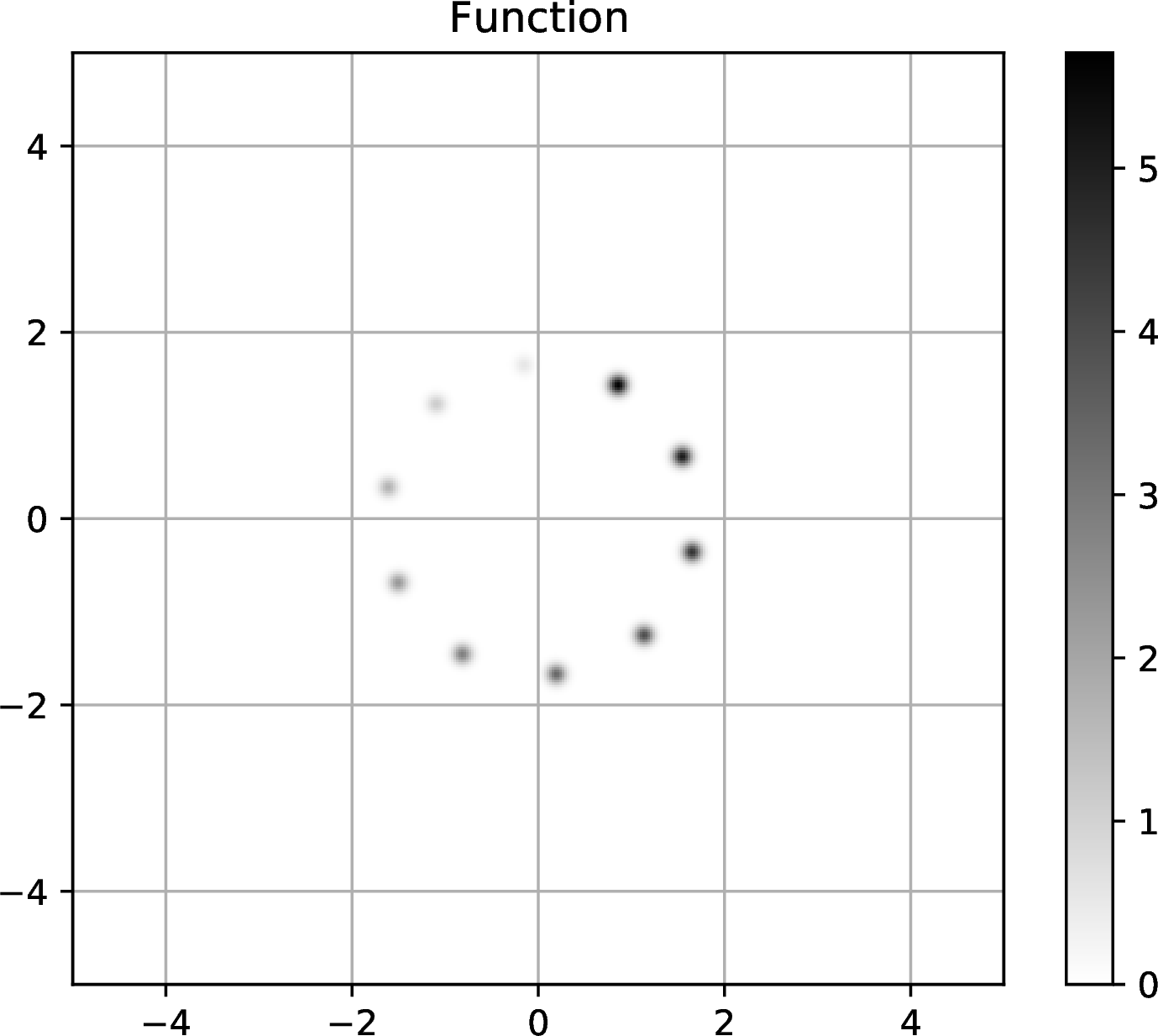
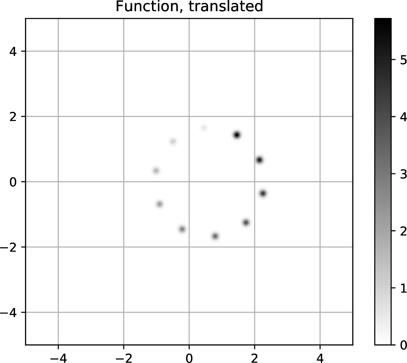
Figure 1: The function \(f\) described in Section 7.1, and its translation by \(0.6\) to the right..

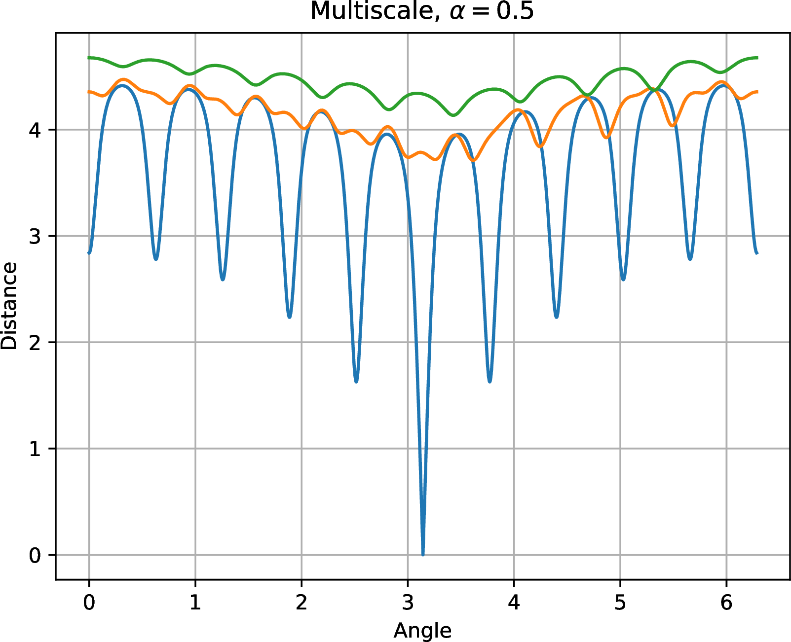
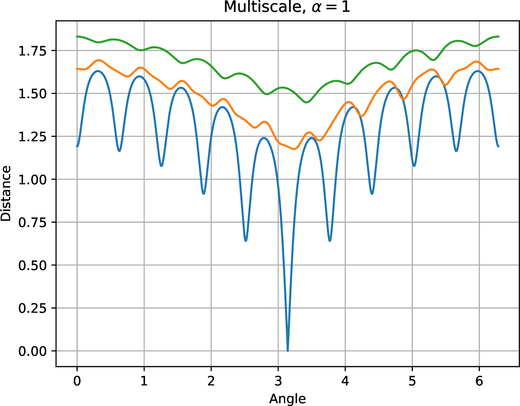
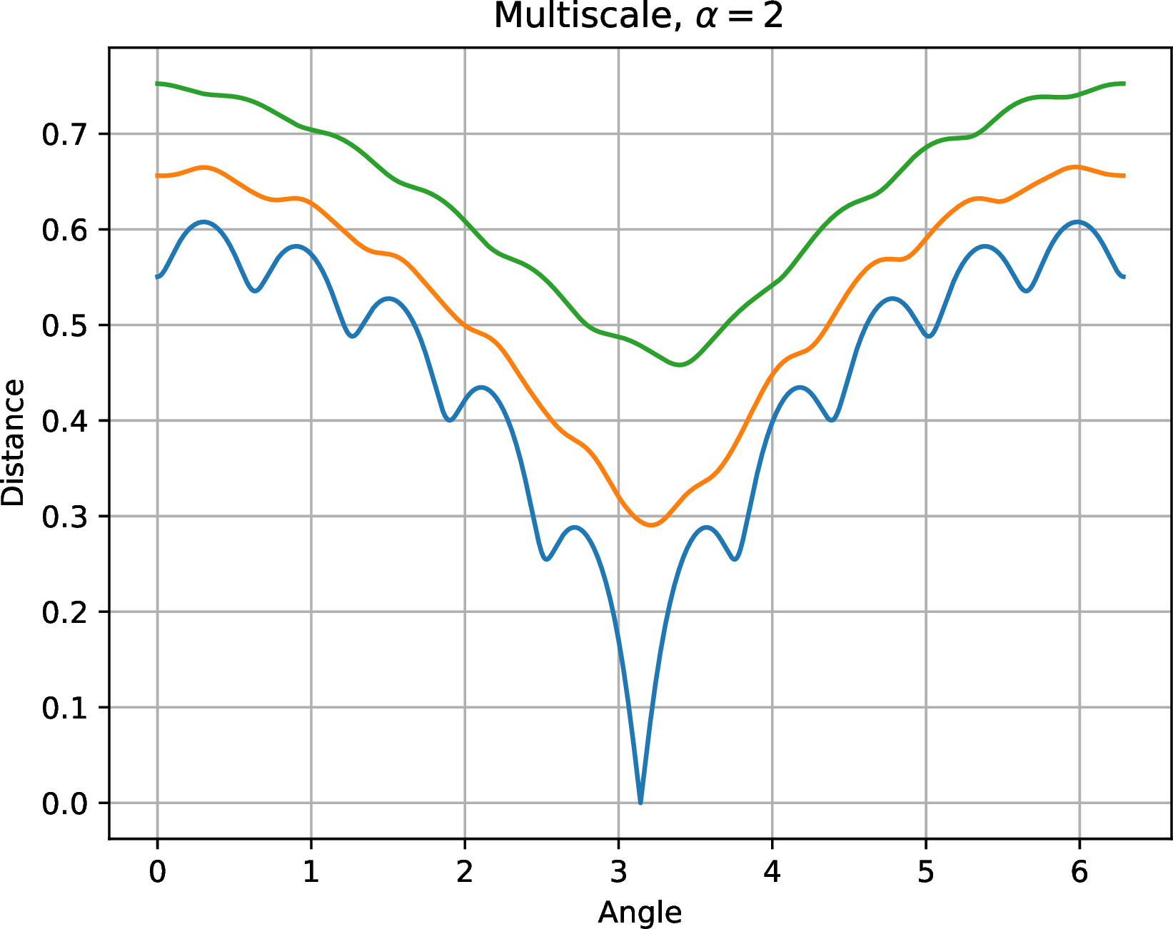
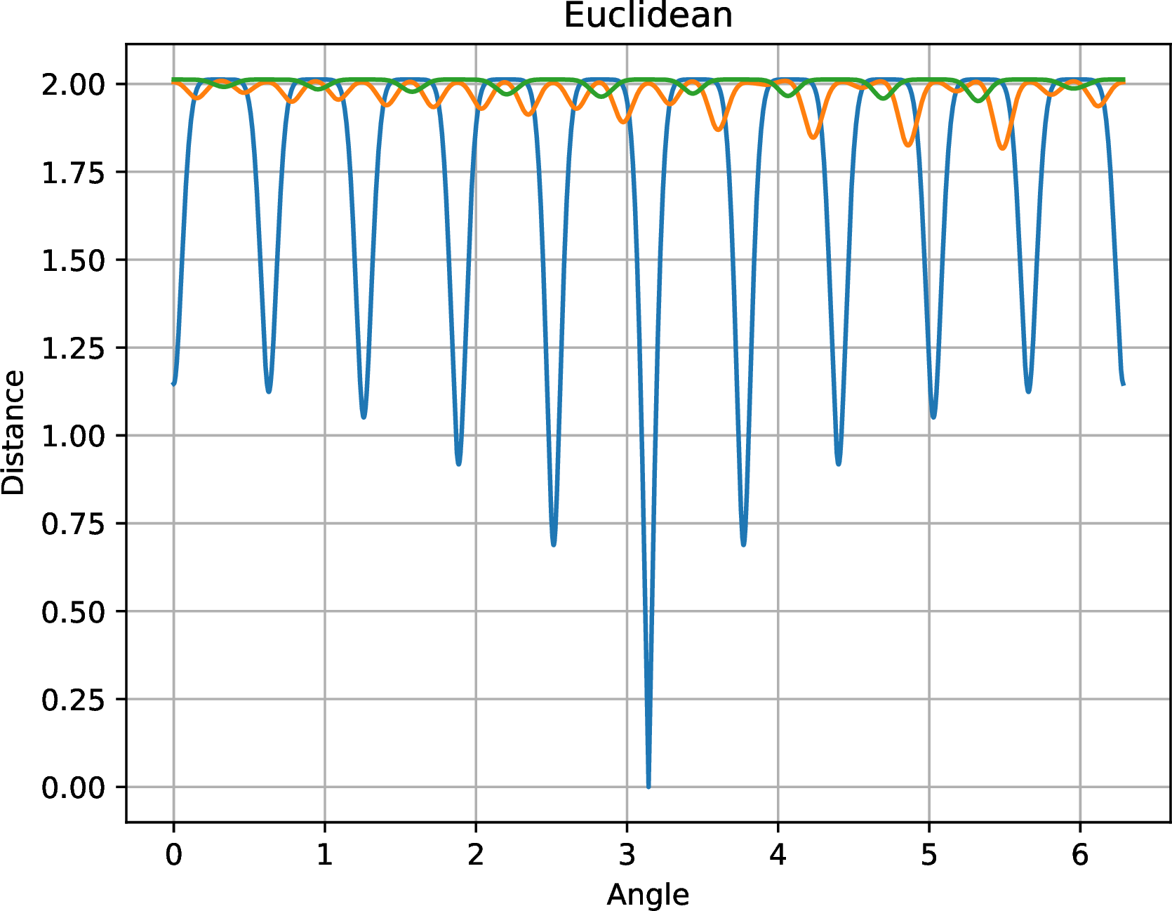
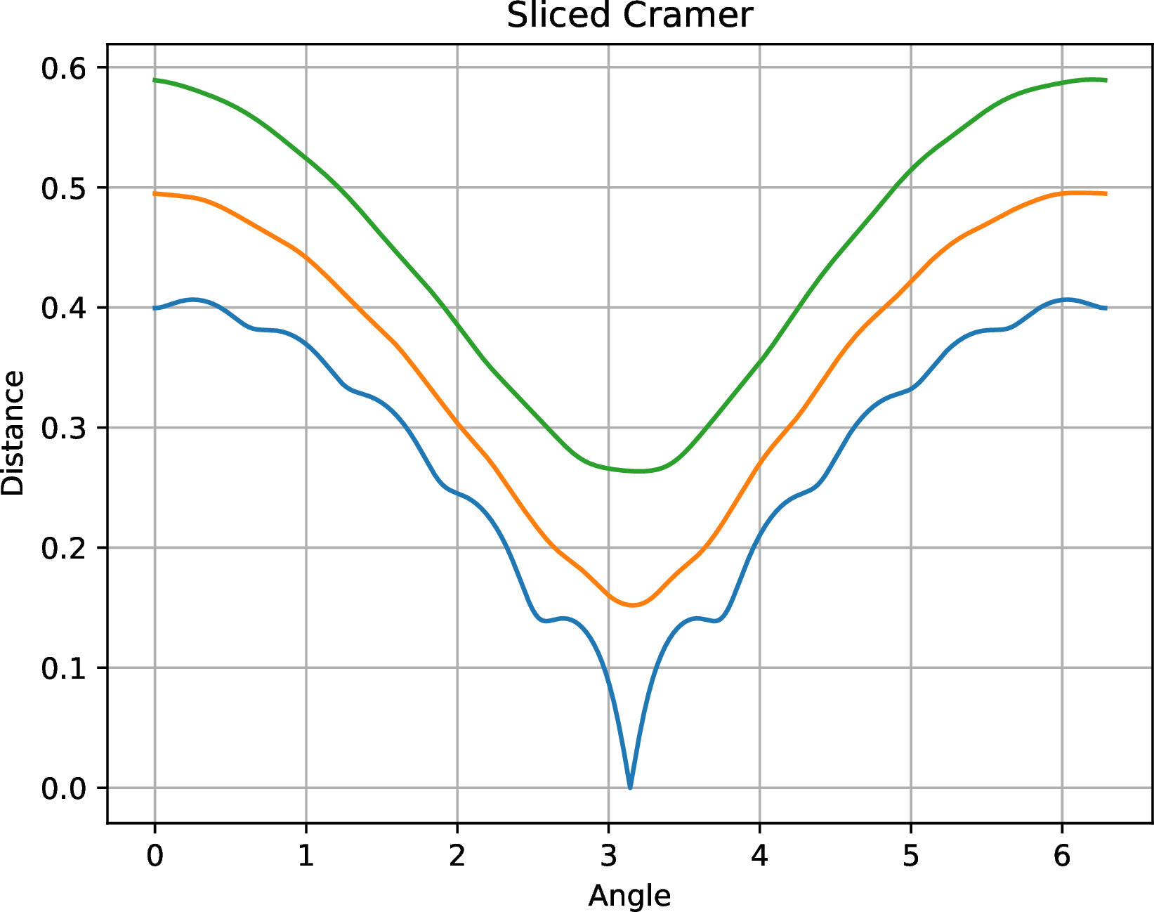
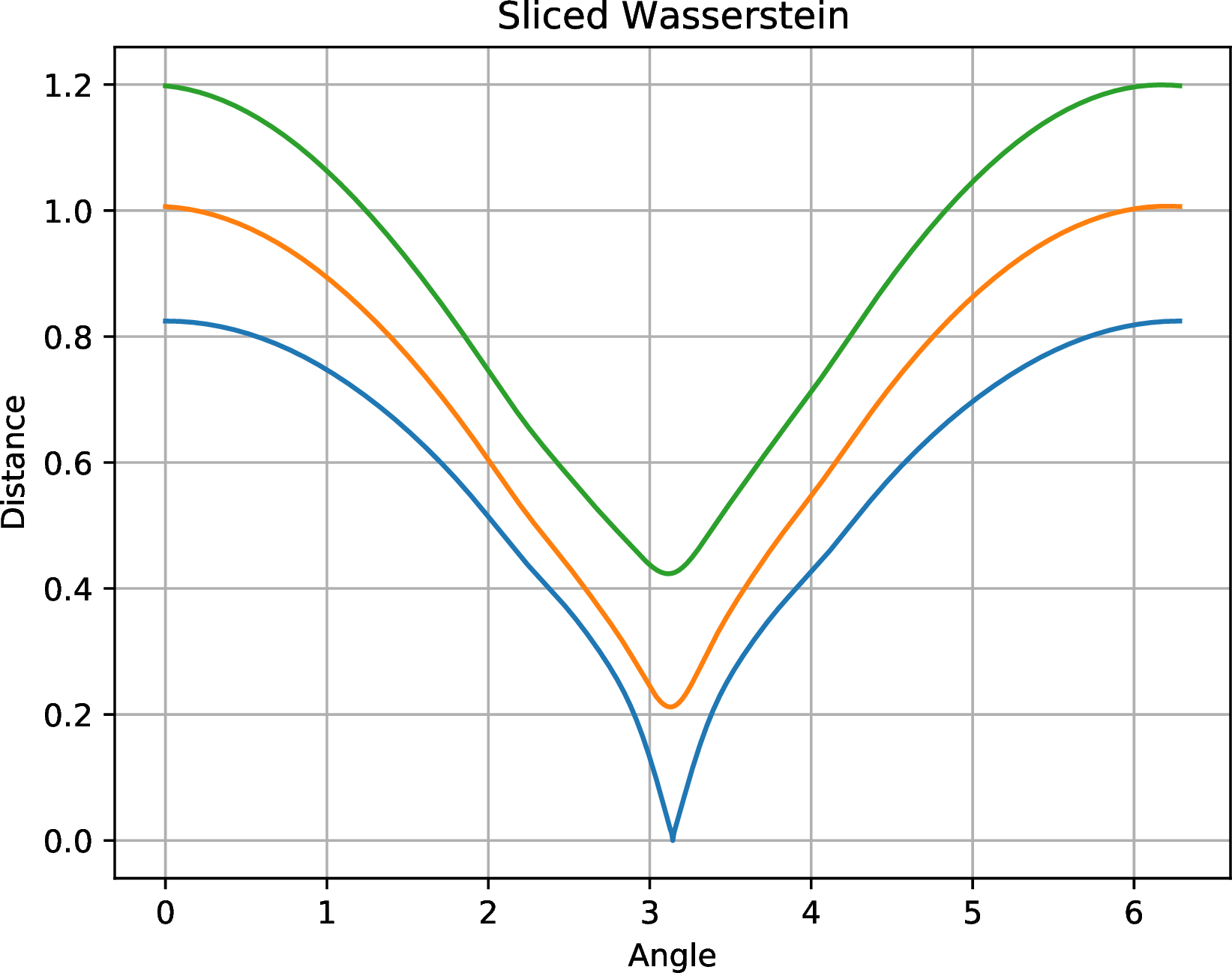
Figure 2: Distances for the experiment described in Section 7.1. From top to bottom, left to right: \(\mathrm{D}_{1/2}\), \(\mathrm{D}_{1}\), \(\mathrm{D}_{2}\), Euclidean, sliced Cramér, and sliced Wasserstein. The blue lines are the distances between the function and itself (rotated by \(\pi\) radians so the minimum value of \(0\) occurs in the middle of the plot); the orange lines are the distances between the function and its translation by \(0.3\); the green lines are the distances between the function and its translation by \(0.6\)..

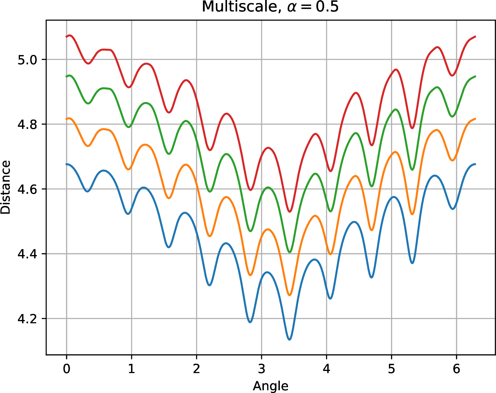
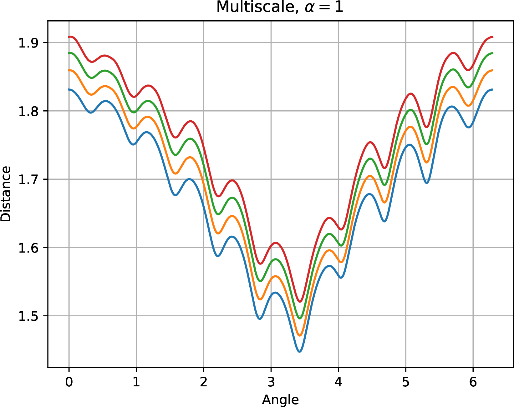
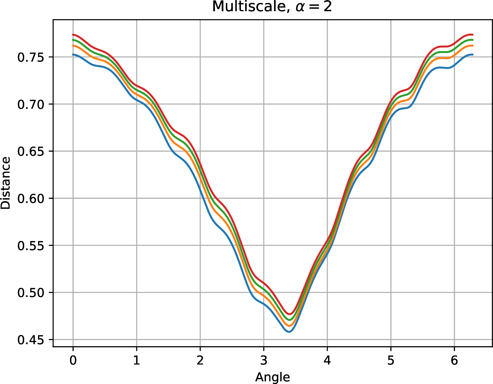
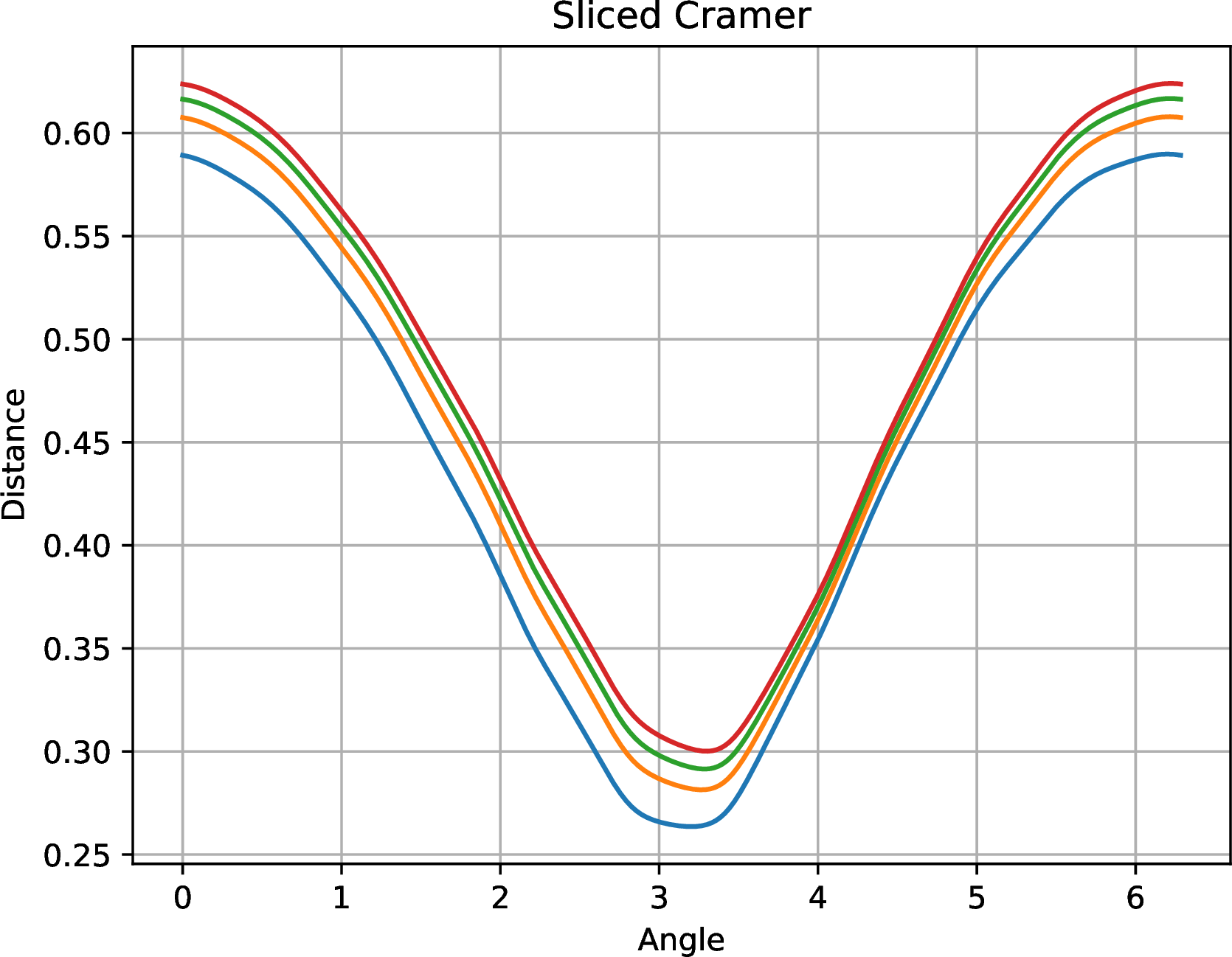
Figure 3: Distances for the experiment described in Section 7.2. From top to bottom, left to right: \(\mathrm{D}_{1/2}\), \(\mathrm{D}_{1}\), \(\mathrm{D}_{2}\), Euclidean, and sliced Cramér. The blue lines are the distances between the function and itself (rotated by \(\pi\) radians so the minimum value of \(0\) occurs in the middle of the plot); the orange lines are the distances between the functions with noise of maximum variance \(0.5\); the green lines are the distances between the functions with noise of maximum variance \(1\); the red lines are the distances between the functions with noise of maximum variance \(1.5\)..

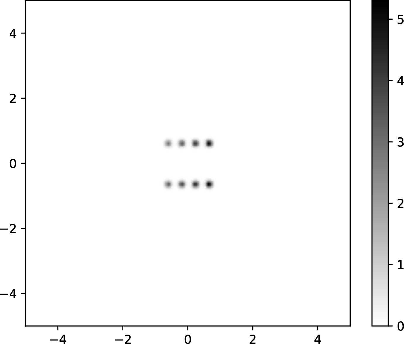
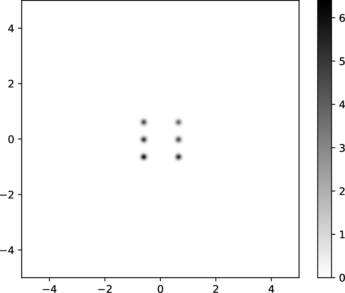
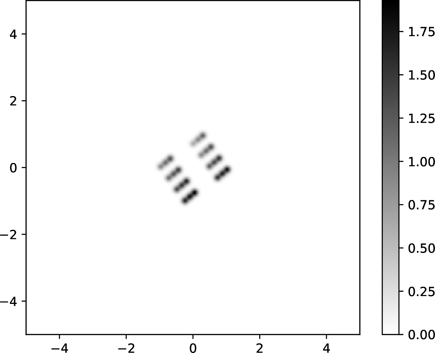
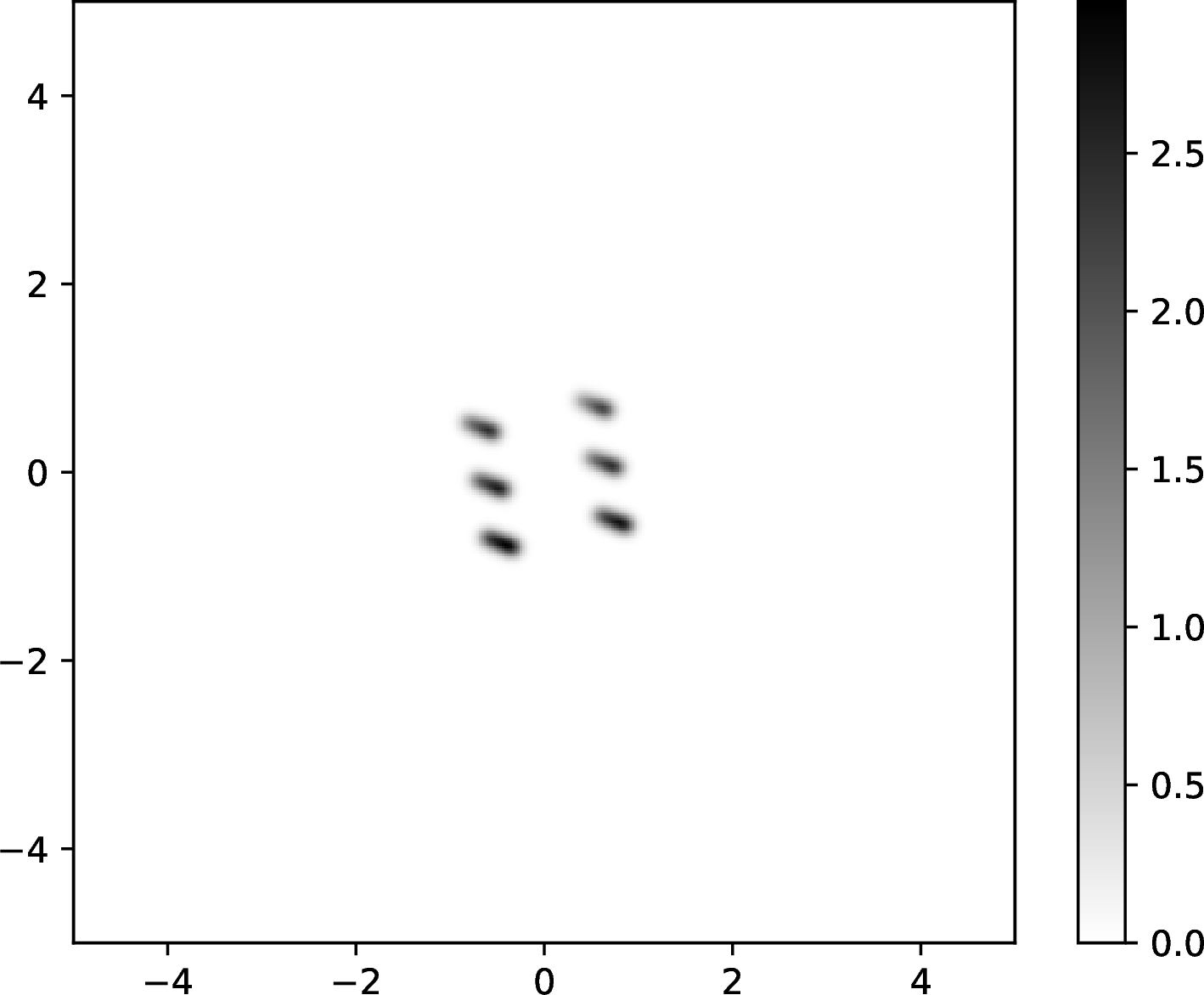
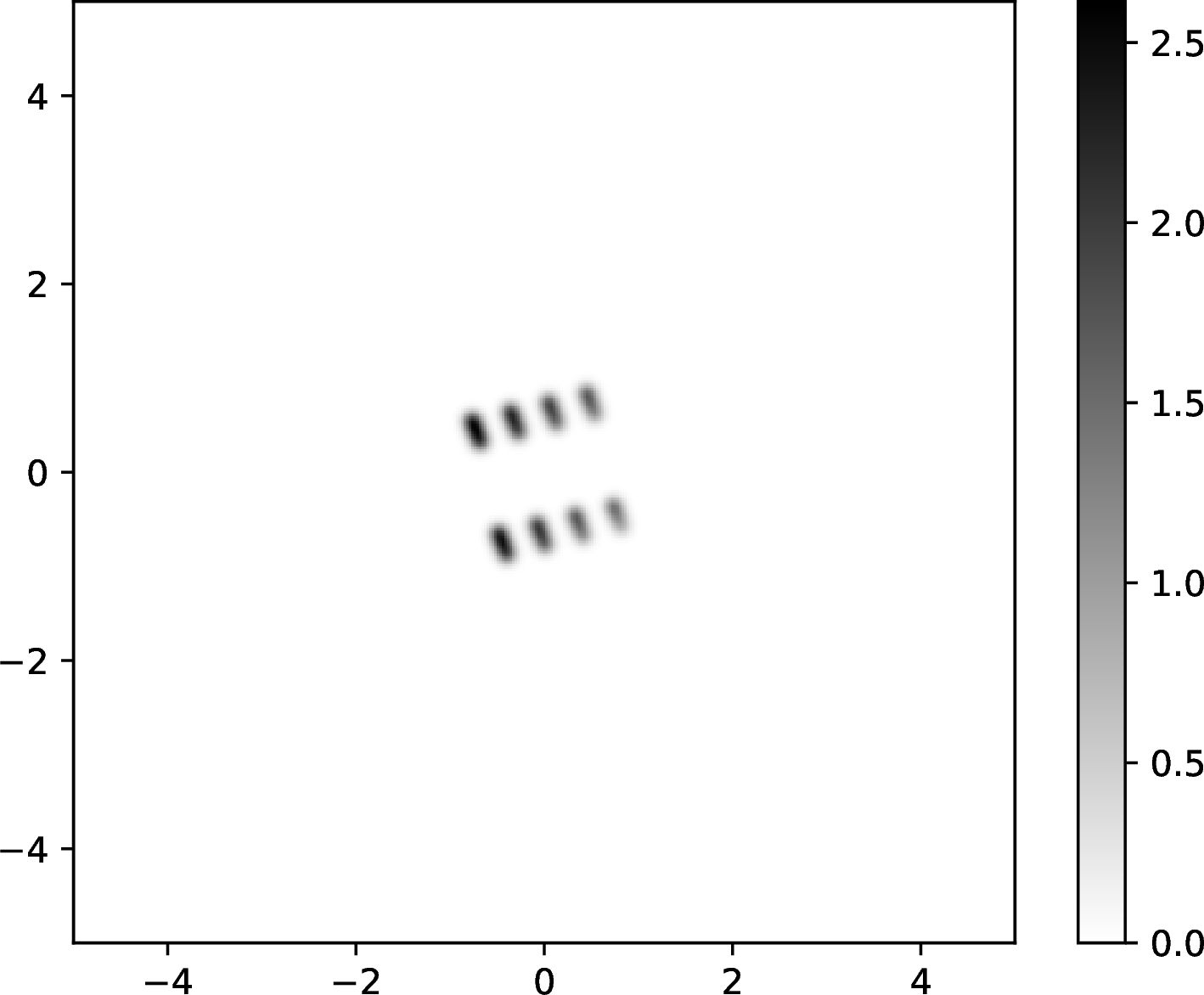
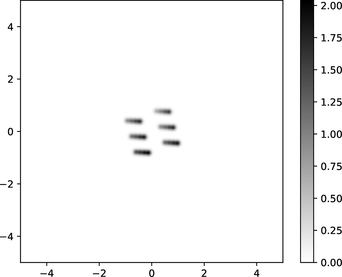
Figure 4: Projections of \(f\) from the experiment described in Section 7.3. Left column: the projection \(g\), and two projections of \(f\) within angle \(\theta\) of \(u_g\). Right column: projection \(h\), and two projections of \(f\) within angle \(\theta\) of \(u_h\). Here, \(\theta = 3 \pi / 20\), and the projections are shown without noise..

Figure 5: Error plot from the experiment described in Section 7.3.

Figure 6: Error plot from the experiment described in Section 7.3, with noise of standard deviation 0.1. — Figure 6: Error plot from the experiment described in Section 7.3, with noise of standard deviation \(0.1\).

Figure 7: Error plot from the experiment described in Section 7.3, with noise of standard deviation 0.2. — Figure 7: Error plot from the experiment described in Section 7.3, with noise of standard deviation \(0.2\).

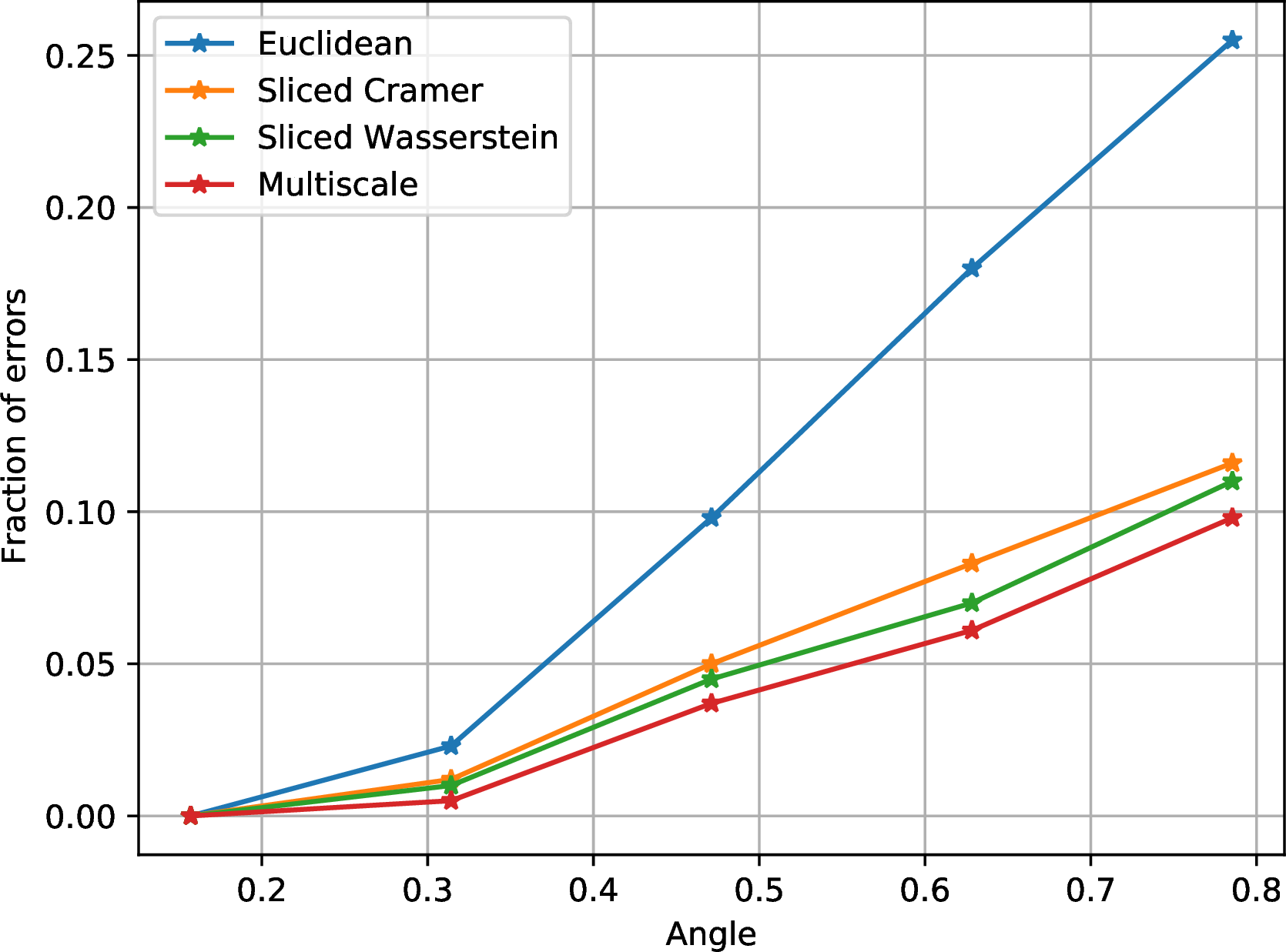
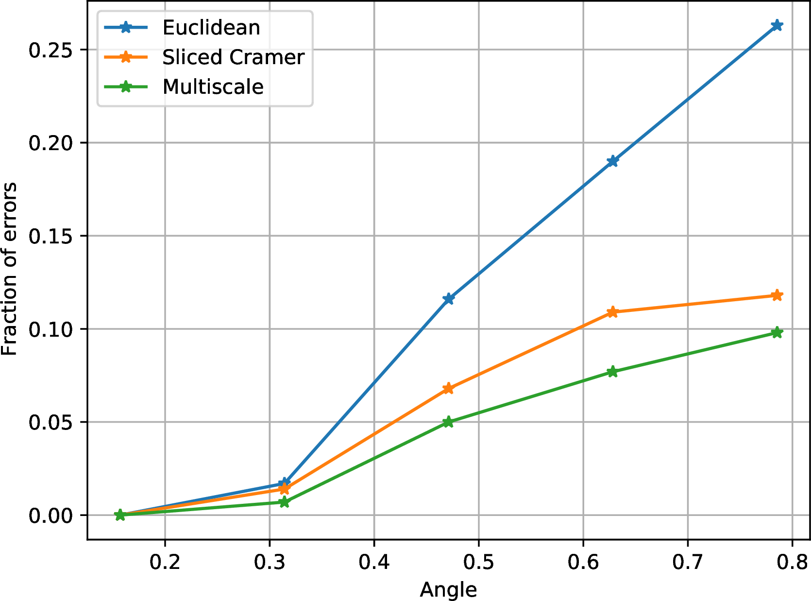
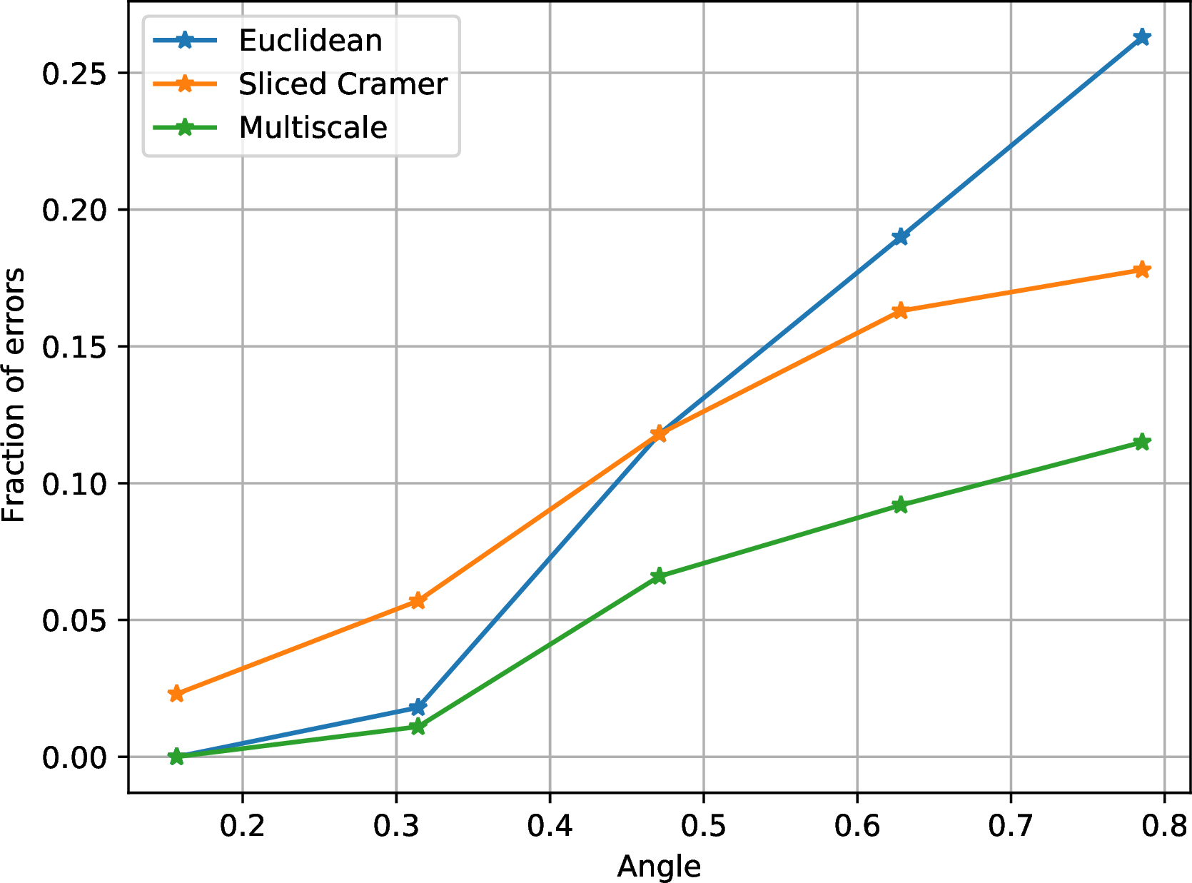
7 Numerical experiments↩︎

We illustrate the performance of the rotationally-invariant metrics \(\mathrm{D}_{\alpha,p}(f,g; \, \mathrm{SO}(2))\) (with \(r=2\)), on several numerical examples. We compare to the rotationally-invariant Euclidean, sliced \(2\)-Cramér, and sliced \(2\)-Wasserstein distances. For simplicity, we take \(p=1\), and denote the metric by \(\mathrm{D}_\alpha\). For our implementations of the rotationally-invariant sliced Wasserstein and sliced Cramér distances, we use similar implementations as those described in [20], though we make use of the obervation from Remark 11 and perform the minimization over a finer grid than the algorithm described in [20]. The code for rotationally-invariant sliced Cramér and sliced Wasserstein distances may be found at github.com/wleeb/SlicedCramer. The code for the multiscale distances \(\mathrm{D}_{\alpha,p}\) (with \(r=2\)), including the rotationally-invariant versions, may be found at github.com/wleeb/Gaussian-Kernel-Metrics.

7.1 Translations and rotations↩︎

We consider the function \(f\), shown in Figure 1, consisting of \(10\) Gaussians arranged equispaced around a circle, of varying heights. Each Gaussian is centered at distance \(5/3\) from the origin, with scale parameter \(1/100\), and heights that grow linearly starting from \(1/55\) and ending at \(10/55\) (the normalization is to ensure the total mass is \(1\)). We evaluate distances between the function shown and all of its rotations, using the fast algorithm described in Section 5.2. We also compute distances between the original function and its translations to the right by \(0.3\) and \(0.6\), respectively. We do this for the distances \(\mathrm{D}_{\alpha}\), \(\alpha = 0.5, 1, 2\) (with \(p=1\)) as well as sliced Wasserstein, sliced Cramér, and Euclidean distance. The distances are shown in Figure 2. As \(\alpha\) grows, the behavior of the distances \(\mathrm{D}_\alpha\) are smoother functions of the rotation angle, similar to the sliced Wasserstein and sliced Cramér distances; whereas for smaller \(\alpha\), \(\mathrm{D}_\alpha\) contains the contours of the Euclidean distance, while still maintaining an overall envelope similar to that of the sliced Wasserstein and sliced Cramér distances.

7.2 Noise and rotations↩︎

We compare the rotations between the two functions shown in Figure 1, where white noise of varying strengths has been added to the rotated function. In this experiment, we do not include the sliced Wasserstein distance, as it is not designed to handle additive noise. The functions are sampled on grids of size \(1592 \times 1592\), which is substantially greater than is needed to resolve the underlying noiseless functions. The variances are, respectively, \(0.5\), \(1.0\), and \(1.5\). As can be seen, the noise drastically inflates the Euclidean distances; because the sample size is so large, the effects on the other metrics are comparatively smaller, and get smaller with larger \(\alpha\), consistent with Theorem 19.

7.3 Projections↩︎

We consider a function \(f\) in 3D, which is a convex combination of 24 Gaussian functions arranged in a \(4\)-by-\(3\)-by-\(2\) grid, each with scale parameter \(1/100\), and heights proportional to \(\sqrt{i^2 + j^2 + k^2}\), where \((i,j,k)\) is the index specifying each Gaussian, with \(i=1,2\), \(j=1,2,3\), and \(k=1,2,3,4\). (The heights are normalized so the total mass is \(1\), making \(f\) a probability density.) The function \(f\) is centered at the origin, with the centers of the Gaussians equally spaced along each dimension, ranging from \(-5/8\) to \(5/8\).

We consider two 2D projections of \(f\), whose axes of projection have angle \(\pi/2\); these two functions, which we call \(g\) and \(h\), are shown in the top row of Figure 4. Denote by \(u_g\) the axis along which \(f\) is projected to generate \(g\), and similarly denote \(u_h\).

In the experiment, for a given angle \(\theta\), we randomly generate two sets of \(500\) projections of \(f\), which we denote \(S_\theta(g)\) and \(S_\theta(h)\), to which we add independent Gaussian noise of variance \(\sigma^2\). Some example projections without noise (\(\sigma=0\)) are shown in the bottom two rows of Figure 4. All the projections in \(S_\theta(g)\) (respectively \(S_\theta(h)\)) are taken at projection axes that lie within \(\theta\) of \(u_g\) (respectively \(u_h\)).

For each projection in \(S_\theta(g)\) and \(S_\theta(h)\), we compute its distances to both \(g\) and \(h\), using the rotationally-invariant versions of the \(\mathrm{D}_{2}\), Euclidean, sliced Cramér, and, in the \(\sigma=0\) case, sliced Wasserstein metrics, and for each distance assign that projection to its nearest center (either \(g\) or \(h\)). For the metric \(\mathrm{D}_2\), we take \(\tau_0 = 25/16\).

In Figure 5, we plot the fraction of incorrectly classified noiseless (\(\sigma=0\)) projections, as the angle \(\theta\) grows, for all four distances. In Figures 6 and 7 we plot the fraction of incorrectly classified projections, for \(\sigma=0.1\) and \(\sigma=0.2\), respectively, as the angle \(\theta\) grows; in these latter two plots, we exclude the sliced Wasserstein metrics, which are not designed to handle additive noise. As one would expect, all errors grow with \(\theta\), since the projections differ more as the angle between them changes.

Interestingly, in all cases the metric \(\mathrm{D}_{2}\) maintains the smallest errors. In the noiseless case, the errors are close to the errors of sliced Cramér and sliced Wasserstein, all three of which are considerably smaller than the errors of Euclidean distance. With non-zero noise, the metric \(\mathrm{D}_2\) performs substantially better than both the Euclidean and sliced Cramér distances. This is suggestive, though by no means conclusive, that the multiscale metric may perform well on the class averaging problem in cryo-EM [21], [48]–[51]; however, additional experimentation is needed that goes beyond the scope of the current paper and will be pursued in future work.

8 Conclusion↩︎

We have shown that the metrics \(\mathrm{D}_{\alpha,p,r}\) are stable to geometric deformations, and that their discretizations are stable under additive noise. We have also introduced rotationally-invariant versions of \(\mathrm{D}_{\alpha,p,2}\), and we have shown that they may be computed efficiently from finite samples. Our numerical results indicate favorable performance compared to the sliced Wasserstein, sliced Cramér, and Euclidean distances.

There are several open questions that we intend to address in future work. Perhaps most straightforward is minimizing the distance over all rigid motions, not just over \(\mathrm{SO}(2)\). While minimizing over translations alone is fairly straightforward (more so than over rotations as we have done in the present work, as it does not require interpolating to a polar grid), simultaneous minimization over all rigid motions is a more challenging task, though we are optimistic that the methods in [52], [53] may be applicable. Second is the question of how to select the parameters \(\alpha\) and \(p\); in particular, larger \(\alpha\) puts more weight on the low-frequency components of the inputs, which makes the metric more stable but may erase critical details in the higher frequencies. On the other hand, larger \(p\) approaches the \(\infty\) norm across scales, which selects a single scale to discriminate the two images, whereas values of \(p\) close to \(1\) incorporate all scales simultaneously. We also intend to extend this work to comparing volumes; Wasserstein-type distances have been proposed for this task in the context of cryo-EM [54], [55], and so it is reasonable to generalize the multiscale metrics studied herein to apply the same class of problems. Finally, Theorem 9 and the experiments in Section 7.3 suggest that in certain cases the rotationally-invariant metrics \(\mathrm{D}_{\alpha,p}\) may be good choices for clustering noisy tomographic images, a task that occurs in the class averaging problem in cryo-EM [21], [48]–[51]; in future work we intend to design and test an end-to-end clustering algorithm for this task.

Acknowledgements↩︎

I acknowledge funding from NSF CAREER award DMS-2238821 and the McKnight Foundation.

References↩︎

[1]

Hans Triebel. Theory of Function Spaces. Birkhäuser, 1983.

[2]

Yoshihiro Sawano. Theory of Besov Spaces. Springer, 2018.

[3]

Tony Lindeberg. Scale-space theory: a basic tool for analyzing structures at different scales. International Journal of Computer Vision, 21(1-2):225–270, 1994.

[4]

David G. Lowe. Distinctive image features from scale-invariant keypoints. International Journal of Computer Vision, 60(2):91–110, 2004.

[5]

David G. Lowe. Object recognition from local scale-invariant features. In Proceedings of the Seventh IEEE International Conference on Computer Vision, volume 2, pages 1150–1157. IEEE, 1999.

[6]

William Leeb and Ronald Coifman. Hölder-Lipschitz norms and their duals on spaces with semigroups, with applications to Earth Mover’s Distance. Journal of Fourier Analysis and Applications, 22(4):910–953, 2016.

[7]

Shirdhonkar Shirdhonkar and David W. Jacobs. Approximate earth mover’s distance in linear time. In IEEE Conference on Computer Vision and Pattern Recognition, pages 1–8, 2008.

[8]

Katy Craig and Haoqing Yu. Wavelet \(s\)-wasserstein distances for \(0 < s \le 1\). Sampling Theory, Signal Processing, and Data Analysis, 23(2), 2025.

[9]

William Leeb. The mixed Lipschitz space and its dual for tree metrics. Applied and Computational Harmonic Analysis, 44(3):584–610, 2018.

[10]

William Leeb. Approximating snowflake metrics by trees. Applied and Computational Harmonic Analysis, 45(2):405–424, 2018.

[11]

Gal Mishne, Ronen Talmon, Israel Cohen, Ronald R. Coifman, and Yuval Kluger. Data-driven tree transforms and metrics. IEEE Transactions on Signal and Information Processing Over Networks, 4(3):451–466, 2017.

[12]

Gal Mishne, Ronen Talmon, Ron Meir, Jackie Schiller, Maria Lavzin, Uri Dubin, and Ronald R. Coifman. Hierarchical coupled-geometry analysis for neuronal structure and activity pattern discovery. IEEE Journal of Selected Topics in Signal Processing, 10(7):1238–1253, 2016.

[13]

Ya-Wei Eileen Lin, Ronald Coifman, Gal Mishne, and Ronen Talmon. . In Advances in Neural Information Processing Systems, volume 38, pages 173762–173822, 2026.

[14]

Moses S. Charikar. Similarity estimation techniques from rounding algorithms. In Proceedings of the Thirty-fourth Annual ACM Symposium on Theory of Computing, pages 380–388, 2002.

[15]

Tamir Bendory, Alberto Bartesaghi, and Amit Singer. Single-particle cryo-electron microscopy: Mathematical theory, computational challenges, and opportunities. IEEE Signal Processing Magazine, 37(2):58–76, 2020.

[16]

Amit Singer and Fred J. Sigworth. Computational methods for single-particle electron cryomicroscopy. Annual Review of Biomedical Data Science, 3:163–190, 2020.

[17]

Marin van Heel, Brent Gowen, Rishi Matadeen, Elena V Orlova, Robert Finn, Tillmann Pape, Dana Cohen, Holger Stark, Ralf Schmidt, Michael Schatz, et al. Single-particle electron cryo-microscopy: towards atomic resolution. Quarterly Reviews of Biophysics, 33(04):307–369, 2000.

[18]

Allison Doerr. Single-particle cryo-electron microscopy. Nature Methods, 13(1):23, 2016.

[19]

Miloš Vulović, Raimond BG Ravelli, Lucas J. van Vliet, Abraham J. Koster, Ivan Lazić, Uwe Lücken, Hans Rullgård, Ozan Öktem, and Bernd Rieger. Image formation modeling in cryo-electron microscopy. Journal of Structural Biology, 183(1):19–32, 2013.

[20]

Yunpeng Shi, Amit Singer, and Eric J. Verbeke. . arXiv preprint arXiv:2503.13756, 2025.

[21]

Rohan Rao, Amit Moscovich, and Amit Singer. Wasserstein k-means for clustering tomographic projections. In NeurIPS 2020, Machine Learning for Structural Biology (MLSB) Workshop, 2020.

[22]

Carlo Tomasi Rubner, Yossi and Leonidas J. Guibas. The Earth Mover’s Distance as a metric for image retrieval. International Journal of Computer Vision, 40(2):99–121, 2000.

[23]

Julien Rabin, Gabriel Peyré, Julie Delon, and Marc Bernot. Wasserstein barycenter and its application to texture mixing. In International Conference on Scale Space and Variational Methods in Computer Vision, pages 435–446. Springer, 2011.

[24]

Nicolas Bonneel, Julien Rabin, Gabriel Peyré, and Hanspeter Pfister. . Journal of Mathematical Imaging and Vision, 51:22–45, 2015.

[25]

Elizaveta Levina and Peter Bickel. The Earth Mover’s Distance is the Mallows Distance: Some insights from statistics. In Proceedings of the Eighth IEEE International Conference on Computer Vision, volume 2, pages 251–256. IEEE, 2001.

[26]

Cédric Villani. Topics in Optimal Transportation, volume 58 of Graduate Studies in Mathematics. AMS, 2001.

[27]

Cédric Villani. Optimal Transport: Old and New. Springer, 2008.

[28]

Filippo Santambrogio. Optimal Transport for Applied Mathematicians: Calculus of Variations, PDEs, and Modeling. Birkhäuser, 2015.

[29]

Gabriel Peyré and Marco Cuturi. Computational optimal transport: With applications to data science. Foundations and Trends in Machine Learning, 11(5-6):355–607, 2019.

[30]

David Marr and Ellen Hildreth. Theory of edge detection. Proceedings of the Royal Society of London. Series B. Biological Sciences, 207:187–217, 1980.

[31]

Hugh R. Wilson and Stephen C. Giese. Threshold visibility of frequency gradient patterns. Vision Research, 17:1177–1190, 1977.

[32]

Peter J. Burt and Edward H. Adelson. The Laplacian pyramid as a compact image code. IEEE Transactions on Communications, 31(4):532–540, 1983.

[33]

Loukas Grafakos. Classical Fourier Analysis. Springer, third edition, 2010.

[34]

William Leeb. On sliced Cramér metrics. arXiv preprint arXiv:2508.02678v2, 2025.

[35]

Stéphane Mallat. Group invariant scattering. Communications on Pure and Applied Mathematics, 65(10):1331–1398, 2012.

[36]

Joakim Andén and Stéphane Mallat. Deep scattering spectrum. IEEE Transactions on Signal Processing, 62(16):4114–4128, 2014.

[37]

Gabor T. Herman. Fundamentals of Computerized Tomography: Image Reconstruction from Projections. Springer Science & Business Media, 2009.

[38]

Gerald B. Folland. Real Analysis: Modern Techniques and Their Applications. John Wiley and Sons, second edition, 1999.

[39]

Ruichong Zhang. . arXiv preprint arXiv:2307.06753, 2023.

[40]

Alex Barnett, Leslie Greengard, Andras Pataki, and Marina Spivak. . SIAM Journal on Imaging Sciences, 10(3):1170–1195, 2017.

[41]

Alex H. Barnett. Aliasing error of the \(\exp(\beta\sqrt{1- z^2})\) kernel in the nonuniform fast Fourier transform. Applied and Computational Harmonic Analysis, 51:1–16, 2021.

[42]

Alexander H. Barnett, Jeremy Magland, and Ludvig af Klinteberg. A parallel nonuniform fast fourier transform library based on an “exponential of semicircle” kernel. SIAM Journal on Scientific Computing, 41(5):C479–C504, 2019.

[43]

Alok Dutt and Vladimir Rokhlin. Fast Fourier transforms for nonequispaced data. SIAM Journal on Scientific Computing, 14(6):1368–1393, 1993.

[44]

Alok Dutt and Vladimir Rokhlin. Fast Fourier transforms for nonequispaced data, II. Applied and Computational Harmonic Analysis, 2(1):85–100, 1995.

[45]

Leslie Greengard and June-Yub Lee. Accelerating the nonuniform fast Fourier transform. SIAM Review, 46(3):443–454, 2004.

[46]

Jeffrey A. Fessler and Bradley P. Sutton. Nonuniform fast Fourier transforms using min-max interpolation. IEEE Transactions on Signal Processing, 51(2):560–574, 2003.

[47]

Roman Vershynin. High-Dimensional Probability: An Introduction with Applications in Data Science. Cambridge University Press, 2nd edition, 2025. Free online edition, available at the author’s website.

[48]

Wooram Park, Charles R. Midgett, Dean R. Madden, and Gregory S. Chirikjian. A stochastic kinematic model of class averaging in single-particle electron microscopy. The International Journal of Robotics Research, 30(6):730–754, 2011.

[49]

Ronny Hadani and Amit Singer. Representation theoretic patterns in three-dimensional cryo-electron microscopy ii –the class averaging problem. Foundations of Computational Mathematics, 11:589–616, 2011.

[50]

Tejal Bhamre, Zhizhen Zhao, and Amit Singer. . In IEEE 14th International Symposium on Biomedical Imaging, pages 654–658. IEEE, 2017.

[51]

Zhizhen Zhao and Amit Singer. . Journal of Structural Biology, 186(1):153–166, 2014.

[52]

Aaditya Rangan, Marina Spivak, Joakim Andén, and Alex Barnett. Factorization of the translation kernel for fast rigid image alignment. Inverse Problems, 36(2):024001, 2020.

[53]

Aaditya V. Rangan. Radial recombination for rigid rotational alignment of images and volumes. Inverse Problems, 39(1):015003, 2023.

[54]

Amit Singer and Ruiyi Yang. . Biological Imaging, 4:E5, 2024.

[55]

Nathan Zelesko, Amit Moscovich, Joe Kileel, and Amit Singer. Earthmover-based manifold learning for analyzing molecular conformation spaces. In IEEE 17th International Symposium on Biomedical Imaging, pages 1715–1719. IEEE, 2020.

On the stability of scale-space metrics