Recent work on self-evolving large multimodal models (LMMs) has demonstrated that models can improve their visual reasoning capabilities in a purely unsupervised manner, without relying on human-annotated supervision or externally verified reward
models [1]–[4]. These approaches frame multimodal reasoning as a self-improving process,
instantiating proposer–solver or questioner–reasoner roles within a shared backbone and reinforcing multi-sample agreement, trajectory-aware feedback, and tool-assisted verification to promote more reliable reasoning [1]–[3], [5]. Despite their promise, however, these methods optimize for answer agreement
without ensuring the decoder attends to the actual visual content, relying instead on statistical language priors to produce self-consistent outputs. This leads to a persistent failure mode we term visual under-conditioning, which causes
hallucination, modality bypass, and unstable visual interpretation even when the vision encoder produces accurate representations. Concretely, this manifests as insufficient attention to visual tokens during decoding, where generations are driven more by
language priors than by the image being described.
This limitation arises from two structural features common to existing self-evolving frameworks. First, the Proposer–Solver setup forms an implicit minimax game: the roles are optimized jointly with opposing objectives, making training unstable over
long horizons. In practice, one role often dominates; Proposer collapses to trivial or degenerate queries that guarantee agreement, or the Solver overfits to the Proposer’s distribution and fails to generalize, driving the system into local minima that are
difficult to correct without external intervention. Second, framing the reward around answer correctness implicitly assumes that self-consistency implies correct visual grounding. A decoder exploiting language priors can achieve high answer agreement
through statistical co-occurrences alone, leaving visual under-conditioning unaddressed or even reinforced.
As illustrated in Fig. 1, this failure mode is directly observable. On chart-based or structured scientific queries, prior self-evolving methods produce the same correct answers as ours, suggesting that the required visual
cues may be sparse or quickly resolved, after which the decoder can proceed largely from its internal representations. However, on natural scene understanding queries such as identifying what a skateboard is actually resting on, these methods default to
statistically common associations (ramp surface, concrete ground), indicating that visual evidence is not being robustly integrated throughout the generation process. In contrast, correctly resolving such cases requires the decoder to remain conditioned on
the specific image content, exposing the gap between answer consistency and genuine visual interpretation. Prior self-evolving methods trained on science- and math-centric images show gains on reasoning benchmarks, yet perform at or below the base model on
captioning and region-level description tasks that require detailed visual conditioning. This disparity validates the hypothesis that improvements in answer agreement do not translate into stronger visual interpretation, and that visual under-conditioning
persists in existing self-evolving frameworks.
To directly address this, we propose VISE (Visual Invariance Self-Evolution), a purely unsupervised self-evolving framework that regularizes the model’s visual
conditioning policy rather than answer agreement. Unlike prior multi-role formulations, VISE operates within a single model, motivated by the observation that a well-pretrained LMM already possesses sufficient knowledge to formulate meaningful queries
about its visual content. Its training signal comes from two complementary invariance-based rewards: a geometric invariance reward that enforces spatial consistency under known transformations, and a semantic invariance reward that
requires the model to recognize the absence of evidence when predicted regions are perturbed. Training on raw images with no annotations, metadata, or external reward models, VISE achieves gains of up to \(+16.85\) CIDEr on
COCO and \(+19.66\) CIDEr on TextCaps, reduces object hallucination (Chair-I) by \(5.0\) points, and improves consistently across VQA and reasoning benchmarks, demonstrating that stronger
visual conditioning generalizes across tasks rather than trading off against them. Mechanistically, VISE achieves this by increasing attention to visual tokens across decoder layers during generation, reflecting the shift from language-prior-driven to
image-conditioned decoding.
In summary, our main contributions are as follows:
We introduce VISE, a single-model, fully unsupervised self-evolving framework that directly addresses visual under-conditioning in LMMs by regularizing the model’s visual conditioning policy rather than its answer agreement, requiring no
annotations, metadata, or external reward models.
We propose two complementary invariance-based reward signals: geometric invariance and semantic invariance via regional perturbation (ghosting), that jointly enforce spatial consistency and evidence sensitivity, providing a purely self-supervised
objective defined entirely from the model’s own predictions.
We empirically validate VISE across 18 benchmarks spanning image captioning, VQA, reasoning, and hallucination on multiple model scales and four backbone families, demonstrating consistent and substantial improvements over all self-evolving
baselines with no tradeoffs between task groups.
Figure 1: Overview of VISE compared to prior self-evolving methods.[1]–[4](Left) Prior approaches use separate roles with role-specific objectives optimized for answer consistency, whereas our VISE operates within a single model using geometric and semantic invariance rewards.
(Right) For chart-based queries that require minimal visual dependence, both the prior method and our VISE provide accurate answers. However, on real-scene understanding tasks that require deeper visual semantics, prior approaches struggle, likely
because the language decoder resorts to statistically plausible scenarios (a “ramp surface” instead of a “metal ledge”). In contrast, VISE accurately identifies the metal ledge, likely due to learning self-consistent visual invariance during unsupervised
training. Additional examples are provided in the suppl. material.
Early work on self-improving LMMs aimed to reduce reliance on human-annotated data through internal preference and alignment signals. Tan [6] introduce
image-driven self-questioning with diffusion-based rejection for DPO optimization. Wang [7] propose an in-context self-critic with visual metrics to construct
preference pairs without external models. Liu [8] study multimodal self-evolution from a reinforcement learning perspective and introduce entropy-driven exploration
to mitigate saturation. While these approaches reduce annotation dependence, they still rely on structured supervision or curated preference construction, limiting fully autonomous self-improvement.
More recent work has shifted to fully unsupervised self-play frameworks with internally generated rewards, yielding strong gains on structured reasoning benchmarks. EvoLMM [1] introduces a Proposer–Solver formulation optimized with continuous self-consistency rewards to enable co-evolution of question generation and reasoning without annotations. Subsequent extensions refine this paradigm:
iReasoner [3] incorporates trajectory-aware rewards, VisPlay [2] promotes
diversity and difficulty to prevent collapse, and Agent0-VL [5] integrates tool-grounded self-verification. C2-Evo [9] and DoGe [10] further address training instabilities through co-evolutionary data loops and role decoupling
mechanisms.
Limitations. Despite their methodological diversity and strong performance on structured reasoning benchmarks, these approaches optimize answer correctness or reasoning consistency as the primary objective. This implicitly assumes that
self-consistent outputs reflect improved visual understanding, which is an assumption that breaks down under visual under-conditioning, where a model can remain self-consistent and even correct while relying on statistical language priors rather than
visual evidence. VISE addresses this directly by replacing answer-agreement rewards with invariance-based rewards that regularize the model’s visual-conditioning policy itself, operating within a single model on raw unlabeled images without specialist
roles or external reward models.
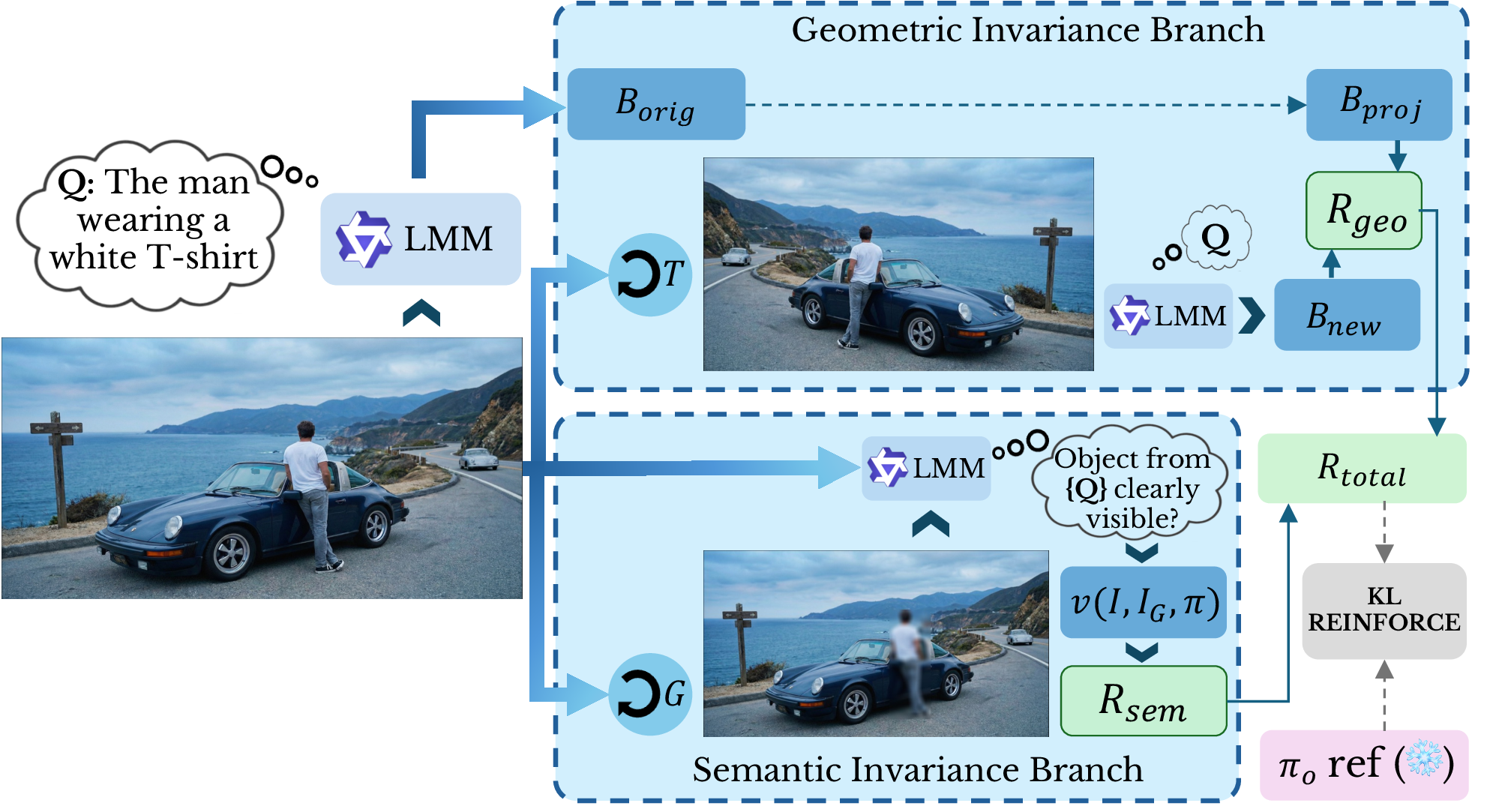
Figure 2: Overview of the VISE self-evolving framework. Given a raw unlabeled image, the model first generates a localization query and predicts a bounding box \(B_\text{orig}\). The Geometric Invariance Branch applies a spatial transformation \(\mathcal{T}\), predicts \(B_\text{new}\) on the transformed view, and
computes \(\mathcal{R}_\text{geo}\) as the GIoU between \(B_\text{new}\) and the projected box \(B_\text{proj}\) to enforce spatial consistency across views.
The Semantic Invariance Branch ghosts the predicted region via blurring and assigns \(\mathcal{R}_\text{sem}\) only if the model detects the object before perturbation and not afterward, penalizing evidence-agnostic
generation. The combined reward is optimized with KL-regularized REINFORCE against a frozen reference policy \(\pi_o\), without annotations, external reward models, or specialist roles.
Problem Formulation. Let \(\mathcal{X} = \{x\}\) denote an unlabeled collection of images, with no accompanying queries, bounding box annotations, or category labels. At each training step, the model
\(\pi_\theta\) operates in a self-questioning regime: it first generates a natural-language localization query \(q\) by interrogating image \(x\), then
predicts a bounding box \(B = (x_1, y_1, x_2, y_2)\) locating the queried object under the same query. Both query generation and bounding box prediction are performed by the same single policy, without separate specialist
roles, as a well-pretrained LMM already possesses sufficient visual knowledge to formulate meaningful queries for its own content. All spatial coordinates are represented in a normalized space \([0, S]^4\), where \(S = 1000\), such that a pixel-space coordinate \(c_\text{pix}\) along dimension \(D\) maps to \(\tilde{c} = (c_\text{pix} / D) \cdot
S\).
We use the Qwen3-VL family [11] as the base backbone, freezing the vision encoder and updating the multimodal
projector, feed-forward layers, and decoder attention projections. This is motivated by the nature of the failure mode: the vision encoder already produces strong visual representations, and the problem lies in how the decoder projects and utilizes them.
Propagating noisy, unsupervised reward gradients into the encoder would risk destabilizing representations that are already high quality, without addressing the locus of failure.
Geometric Invariance Reward. Visual under-conditioning manifests most directly in localization instability: a decoder that disengages with visual image evidence will produce predictions that are inconsistent with the actual spatial
structure of the scene, and in particular will fail to maintain coherent localization when the image undergoes a known geometric transformation. We exploit this as a self-supervised training signal. If the model correctly conditions its localization on
what it sees, then its predicted box on a geometrically transformed image should correspond precisely to the analytically projected version of its prediction on the original. Deviation from this consistency is evidence of visual under-conditioning, and we
penalize it directly.
At each training step, the model generates a query \(q\) by conditioning on image \(x\), producing a short natural-language description of a prominent and spatially unambiguous object in
the scene. The model then predicts a bounding box \(B_\text{orig}\) on the image under query \(q\). A geometric transformation \(\mathcal{T}\) is sampled
uniformly from three types: affine (rotation \(\theta \sim \mathcal{U}(-10^\circ,
10^\circ)\), scale \(s \sim \mathcal{U}(0.9, 1.1)\), translation \((\delta_x, \delta_y) \sim \mathcal{U}(-50, 50)^2\)), crop (ratio \(\rho \sim
\mathcal{U}(0.8, 1.0)\), resized to original resolution), or horizontal flip. Each is described by a known \(3{\times}3\) homogeneous matrix \(M\). The model then predicts a second
box \(B_\text{new}\) on the transformed image \(x' = \mathcal{T}(x)\) under the same query \(q\). The expected box under the transformation is computed
by lifting the four corners of \(B_\text{orig}\) to homogeneous coordinates and applying \(M\) as \(\mathbf{c}'_i = M\mathbf{c}_i\); the axis-aligned box
of the resulting corners gives the projected box \(B_\text{proj}\). The geometric invariance reward is:
with \(\mathcal{C}\) denoting the smallest axis-aligned box enclosing both \(B_1\) and \(B_2\). The linear normalization in Eq. (1 ) maps GIoU \(\in [-1, 1]\) to \(\mathcal{R}_\text{geo} \in [0, 1]\). This reward is maximized when the model’s localization on the transformed view agrees
precisely with the geometric projection of its original prediction, and degrades smoothly as spatial consistency deteriorates. In this way, \(\mathcal{R}_\text{geo}\) directly targets the spatial dimension of visual
under-conditioning: such a model cannot maintain such consistency across views and is therefore penalized, even if its individual predictions appear plausible in isolation.
Figure 4 provides representational evidence that \(\mathcal{R}_\text{geo}\) achieves its intended effect. We compute per-layer Centered Kernel Alignment (CKA) similarity [13] between representations of original and geometrically augmented views for the base model and VISE across 100 random COCO images. On Qwen3-VL-2B, gains are confined to the final
decoder layers, localizing geometric under-conditioning to the stages where generation decisions are formed. On Qwen3-VL-4B, the \(\Delta\)CKA advantage is distributed more broadly across the decoder, consistent with the
scale effects in Table 1: concentrated failures yield more direct downstream gains under invariance-based correction.
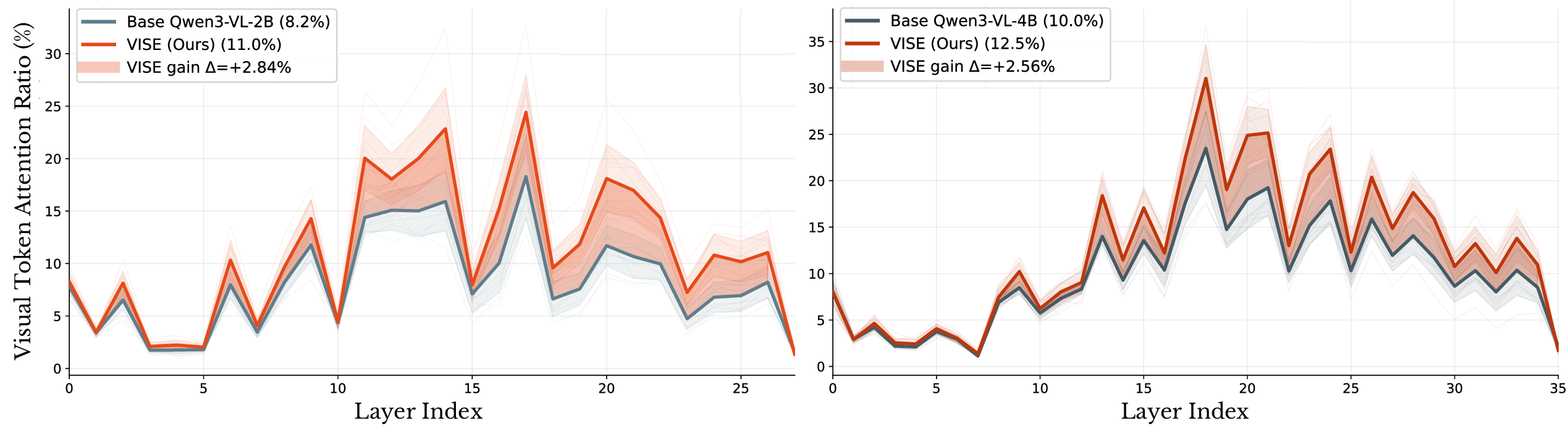
Figure 3: Generation-time visual attention per transformer layer for Base and VISE models on Qwen3-VL-2B (left) and Qwen3-VL-4B (right). VISE-trained models (orange) consistently assign more attention to
image tokens across mid-to-late decoder layers where semantic generation occurs, with mean gains of \(+2.84\%\) and \(+2.56\%\) respectively and per-sample peaks of up to \(+5.09\%\) in layers 15–25. The effect is consistent across both model scales, aligning with our claim that the semantic invariance reward strengthens visual conditioning during generation.
Semantic Invariance Reward. Geometric consistency is a necessary but insufficient condition for faithful visual conditioning. A model could achieve high \(\mathcal{R}_\text{geo}\) by predicting large,
spatially stable regions without its predictions being meaningfully driven by the semantic content they enclose. Hence, we also address the complementary dimension of visual under-conditioning: evidence sensitivity. A model whose responses are
conditioned on the image should recognize that removing the predicted region removes the evidence for the queried object. If instead the decoder is shortcutting from language priors, it would remain insensitive to that removal. We reward the opposite: the
model should judge the object as visible when the region is intact, and as absent when it is obscured.
We do this by introducing a regional perturbation procedure termed ghosting. Given the predicted box \(B_\text{orig}\), the corresponding pixel region in the original image \(x\)
is identified and its contents replaced by a Gaussian-blurred version with kernel \(\sigma = 25.0\), producing a ghosted image \(\tilde{x}\) in which the localized region is visually
degraded while the surrounding context is fully preserved. The model then assesses the visibility of the queried object under \(q\) on both \(x\) and \(\tilde{x}\) via greedy decoding, yielding binary judgments \(v = \texttt{vis}(x, q) \in
\{0, 1\}\) and \(\tilde{v} = \texttt{vis}(\tilde{x}, q) \in \{0, 1\}\). The semantic invariance reward is: \[\mathcal{R}_\text{sem} = \begin{cases} 1.0
& \text{if } v = 1 \;\text{ and }\; \tilde{v} = 0 \\ 0.0 & \text{otherwise} \end{cases} \label{eq:r95sem}\tag{3}\]
Figure 4: Per-layer CKA similarity between original and geometrically augmented views in Qwen3-VL decoder layers. On 2B, VISE gains are confined to final layers (peak \(\Delta=+0.069\) at layer 27) with 100% win-rate. On 4B, gains span layers 19–33 (peak \(\Delta=+0.253\)), with win-rate increasing from \(\sim\)60% at layer 15
to 100% beyond layer 25.
A prediction that is geometrically consistent but semantically arbitrary (enclosing a region that does not contain the queried object) receives \(\mathcal{R}_\text{sem} = 0\) even if it satisfies \(\mathcal{R}_\text{geo}\), ensuring the two signals are complementary and jointly necessary for the model to improve its evidence binding. Figure 3 provides direct evidence of the intended
behavioral change. We measure generation-time visual attention, which is the fraction of attention each generated token assigns to image tokens across transformer layers, for the base model and VISE averaged over 100 random COCO images. Unlike prefill
attention, which is dominated by the visual embedding layer, generation-time attention captures how the decoder references visual evidence while producing each token. VISE consistently assigns more attention to visual tokens across mid-to-late decoder
layers on both model scales, indicating that the semantic invariance reward encourages the decoder to maintain visual conditioning throughout generation rather than reverting to language priors after initial image encoding.
Composite Reward and Optimization. The total reward combines both invariance signals as \(\mathcal{R}_t = \lambda_\text{geo} \mathcal{R}_\text{geo}
+ \lambda_\text{sem} \mathcal{R}_\text{sem}\), where \(\lambda_\text{geo} = \lambda_\text{sem} = 0.5\). At each step, the model produces a completion \(y\) containing the predicted
box coordinates for \((x, q)\). We maintain an exponential moving average baseline \(b_t \leftarrow 0.9\,b_{t-1} +
0.1\,\mathcal{R}_t\) to reduce gradient variance, giving advantage \(A_t = \mathcal{R}_t - b_t\). Letting \(\Delta_t = \log p_\theta(y
\mid x, q) - \log p_\text{ref}(y \mid x, q)\) denote a KL-like divergence proxy between the current policy and the frozen reference \(\pi_\text{ref}\), we optimize:
where the first term is a REINFORCE-style update and the second regularizes against the reference model. We adapt the KL Coefficient \(\beta_t\) dynamically to maintain a target divergence level:
where \(\tau = 0.020\) is the target divergence budget, \(\eta = 0.10\) is the adaptation rate, and \(\beta_t\) is clipped below at \(10^{-6}\). This tightens regularization when the policy drifts beyond the target and relaxes it when updates are conservative, providing stable self-evolution without a fixed regularization strength.
Table 1: Evaluation results on fourimage captioning benchmarks.C = CIDEr, M = METEOR, R = ROUGE-L. Consistency-based methods trained on math and scientific images(EvoLMM, iReasoner) regress on captioning across all scales; EvoLMM
drops \(-0.70\) CIDEr on COCO and \(-0.94\) on Flickr30kat 2B, suggesting that prior-driven generation reinforces languagepriors rather than correcting them. Conversely, VISE improves
CIDErfrom \(21.54 \rightarrow 38.39\) on COCO and \(22.20 \rightarrow 41.86\)on TextCaps at 2B, with no regressions across any dataset or scale.
Implementation Details. We fine-tune each base model using LoRA [14] while keeping the vision encoder frozen. For the smaller models (2B and
4B), we use rank \(r{=}16\) and \(\alpha{=}32\), whereas for the larger models (8B and 32B), we increase the rank to \(r{=}32\) and \(\alpha\) to \(64\) (dropout \(0.05\) in all cases). Training uses the AdamW optimizer [15] with weight decay \(0.01\) and gradient clipping at \(1.0\). We set the learning rate to \(10^{-6}\) and the KL
regularization target to \(0.020\) (adaptive rate \(0.10\)) for smaller models, and reduce them to \(1.5\times10^{-7}\) and \(0.004\) (adaptive rate \(0.15\)), respectively, for larger models. Equal reward weights of \(0.5\) are applied to both the geometric and semantic invariance
terms. All models are trained for 4000 steps on 8\(\times\) AMD MI250X GPUs using bfloat16 precision. No question–answer pairs, annotations, metadata, or external reward models are used.
Training Data. We use 4000 raw, unlabeled images sampled from the COCO dataset [16], with no captions, bounding boxes, or semantic labels
retained. Spatial transformations (affine, crop, and flip) are applied online during training to generate geometric invariance targets. Supp. Sec. 8 reports Objects365 training results showing consistent gains
beyond COCO-specific image exposure.
Baselines and Evaluation. We compare against five self-evolving baselines on the same base models: VisPlay [2], EvoLMM [1], and iReasoner [3], which are fully unsupervised and require no external rewards or annotations,
and VisionZero [4] (CLEVR, Chart, and Real-World [RW] variants), where only CLEVR is label-free, while Chart and Real-World use GPT-4o during dataset
construction. All evaluations are run on AMD MI250X GPUs using the lmms-eval framework [17], with HuggingFace Transformers v4.38 and bfloat16 precision for
consistency with training. We evaluate on four image captioning benchmarks (COCO [2014/2017 average] [16], NoCaps [18], Flickr30k [19], TextCaps [20]), twelve VQA and reasoning benchmarks (GQA [21], OK-VQA [22], VQAv2 [23], AI2D [24], ChartQA [25],
InfoVQA [26], ScienceQA [27], MMMU [28], CaptionQA [29], RWQA [30], ESB [31], MMBench [32]), and two hallucination benchmarks (POPE [33] and COCO Cap
Chair [34]).
Image Captioning.
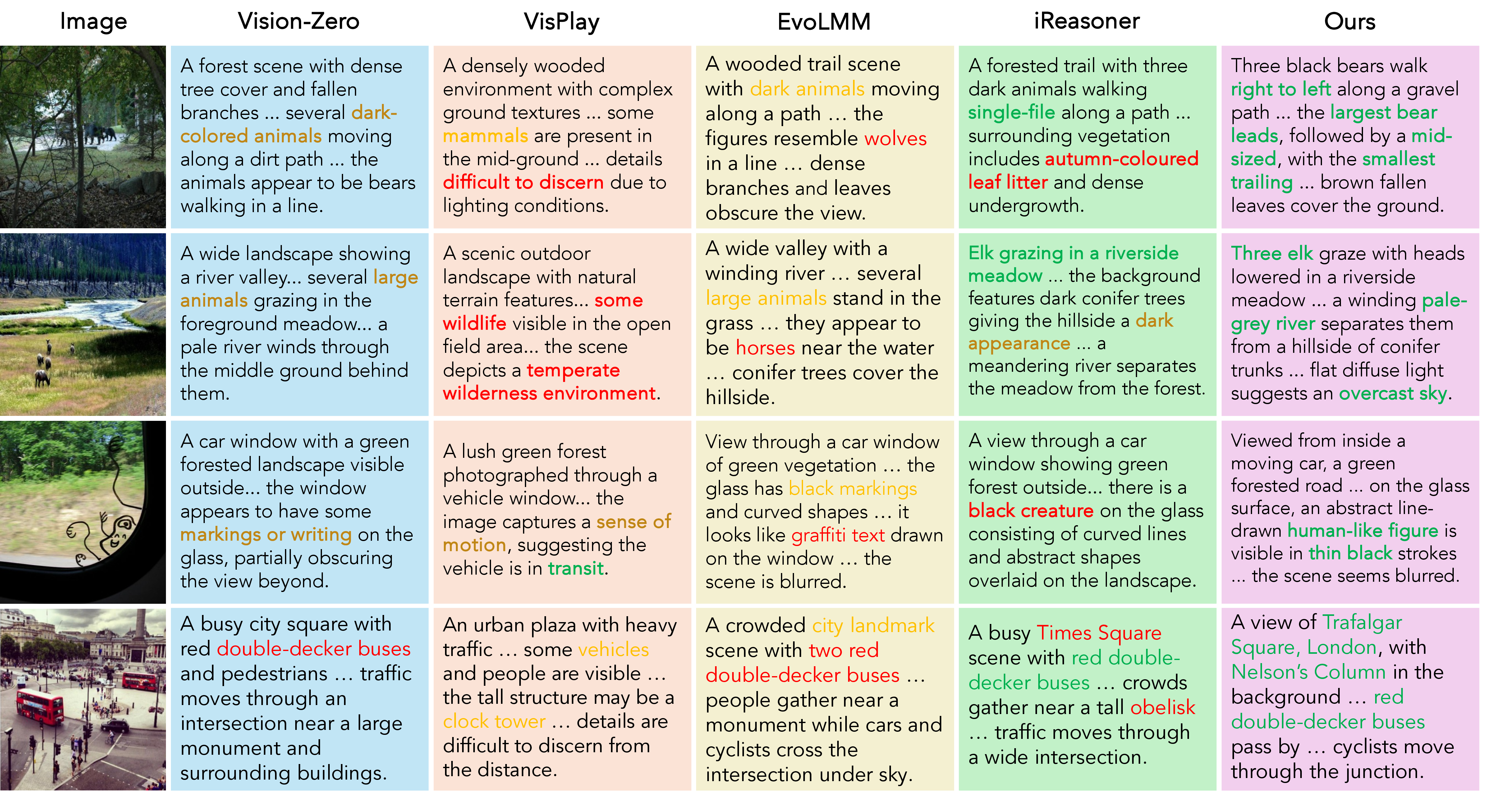
Figure 5: Qualitative comparison of VISE and baselines on four images. Baselines generate either vague category-level descriptions (“large animals,” “vehicles”) or confident hallucinations (“wolves,”
“obelisk”), reflecting reliance on language priors. In contrast, VISE provides specific, image-grounded descriptions: it identifies the three bears by size and position, names the elk and river color, recognizes the human-like figure on the car window, and
correctly identifies Trafalgar Square and Nelson’s Column. These differences are supported by CIDEr gains in Table 1, indicating that invariance-based training encourages reliance on visible evidence rather than
scene-level priors.
In Table 1, we compare VISE against all baselines across four captioning benchmarks and four Qwen3-VL scales. Consistency-based methods trained on math and scientific images show a clear pattern at 2B: EvoLMM drops
\(-0.70\) CIDEr on COCO, \(-0.77\) on NoCaps, and \(-0.94\) on Flickr30k, with iReasoner following a similar trend. This persists across scales, and cannot
be explained by distribution mismatch alone; when answer agreement is the reward, the model is never required to describe what it actually sees, so captioning degrades. VisionZero-RW is the strongest captioning baseline at 2B (\(+4.04\) COCO CIDEr) owing to closer alignment with natural scenes, though its Chart and CLEVR variants show smaller and less consistent gains. VisPlay improves COCO by \(+2.31\) but regresses on
NoCaps (\(-0.38\)) and TextCaps (\(-0.09\)), suggesting diversity and difficulty rewards prioritize question complexity over visual faithfulness. At larger scales, VisionZero variants
recover further (e.g., RW reaches \(+8.41\) COCO CIDEr at 8B) while EvoLMM and iReasoner remain inconsistent, pointing to distribution proximity rather than visual conditioning as the reason.
VISE improves CIDEr on Qwen3-VL-2B by \(+16.85\) on COCO, \(+14.73\) on NoCaps, \(+16.55\) on Flickr30k, and \(+19.66\)
on TextCaps with gains \(4{\times}\)–\(7{\times}\) larger than the strongest baseline on each benchmark and no regressions across any dataset or scale. Gains decrease with model size (\(+16.85\) at 2B to \(+8.72\) at 32B on COCO), in line with larger models entering training with stronger visual conditioning already consolidated during pretraining. Figure 5 shows what these numbers look like in practice. Where baselines either stay vague ("large animals near a river") or commit to plausible-but-wrong details ("wolves," "obelisk"), VISE reads the image: it catches that the
animals are three bears of different sizes walking in order, that there is a hand-drawn figure on the car window, and that the square is Trafalgar rather than a generic city landmark. The gap between these outputs is precisely what the CIDEr gap in
Table 1 reflects.
Table 2: Evaluation results ontwelve VQA and reasoning benchmarks. All valuesare Accuracy except CaptionQA (GPT Score). Domain-specific baselinesexhibit a consistent generalization tradeoff: EvoLMM and iReasoner improveon
ScienceQA (\(+3.59\), \(+3.70\)) but drop on OK-VQA (\(-2.73\), \(-2.63\)),while VisionZero variants show the reverse
pattern depending on trainingdomain. VISE improves all twelve benchmarks simultaneously at 2B(\(+4.19\) ScienceQA, \(+2.41\) InfoVQA, \(+1.75\) MMMU) with no
regressionsat any scale, demonstrating that strengthening visual groundinggeneralizes across task formats without domain-specific adaptation.
VQA and Reasoning. Table 2 reports performance across twelve VQA and reasoning benchmarks. The baseline results exhibit a consistent generalization tradeoff that is not observed with VISE. VisionZero-Chart
improves ChartQA by \(+0.96\) at 2B but drops \(-0.45\) on OK-VQA and \(-0.50\) on CaptionQA; VisionZero-RW shows the reverse, gaining on natural-language
tasks (\(+0.90\) RWQA) but dropping on ChartQA (\(-0.47\)); VisionZero-CLEVR improves structured reasoning (\(+2.54\) ScienceQA, \(+1.91\) InfoVQA) while remaining inconsistent on open-ended VQA. This bidirectional pattern suggests that domain-specific consistency training picks up the statistical regularities of the training distribution alongside any
conditioning signal, imposing a ceiling that cannot be lifted without changing the reward itself. EvoLMM and iReasoner follow the same logic: strong gains on ScienceQA (\(+3.59\), \(+3.70\)
at 2B) but drops on OK-VQA (\(-2.73\), \(-2.63\)) and VQAv2 (\(-0.51\), \(-0.43\)), in line with the captioning dips in
Table 1.
Table 3: Evaluation results on POPEand COCO Cap Chair hallucination benchmarks.\(\downarrow\) indicates lower is better. EvoLMM and iReasoner modestly reduce Chair scores (\(-0.23\) Chair-I at2B) but simultaneously drop POPE accuracy (\(-1.42\), \(-1.31\)),indicating inconsistent visual grounding. In contrast, VISE reducesChair-I
from \(13.21 \rightarrow 8.21\) (\(-5.00\)) and Chair-S from\(45.96 \rightarrow 40.51\) (\(-5.45\)) at 2B, surpassing the
strongestbaseline by \(+2.01\) and \(+1.40\), while also improving POPE by\(+1.02\).
VISE improves all twelve benchmarks simultaneously at 2B, with gains of \(+4.19\) on ScienceQA, \(+2.41\) on InfoVQA, \(+1.75\) on MMMU, and \(+2.12\) on CaptionQA, and no regressions at any scale. At 4B, the MMMU gain grows to \(+3.72\), the largest improvement on that benchmark across all methods and scales, indicating that stronger
conditioning particularly benefits tasks requiring multi-discipline visual reasoning. Across all four scales, VISE exhibits no structured-versus-open-ended tradeoff observed in the baselines. Instead of adapting to a specific domain, the invariance reward
improves the model’s visual conditioning behavior, and these improvements generalize across task formats.
Hallucination. Table 3 evaluates all methods on POPE and COCO Cap Chair. VisPlay increases hallucination at 2B (Chair-I \(+0.003\), Chair-S \(+0.23\)), consistent with diversity rewards prioritizing question complexity over visual fidelity. EvoLMM and iReasoner reduce Chair scores modestly (\(-0.23\), \(-1.74\)) but drop POPE accuracy (\(-1.42\), \(-1.31\)) simultaneously. Sentence-level hallucinations decline while binary object-presence reliability weakens,
pointing to inconsistent rather than substantive improvement. VisionZero-RW is the strongest baseline (Chair-I \(-2.99\), Chair-S \(-4.05\)), due to broader real-world visual coverage. VISE
reduces Chair-I by \(-5.00\) and Chair-S by \(-5.45\) at 2B, surpassing the best baseline by \(+2.01\) and \(+1.40\) while
also improving POPE by \(+1.02\). This joint improvement across both metrics is unique to VISE: penalizing confident predictions under regional perturbation discourages generating objects that are statistically plausible
but not visually present. Gains attenuate with model size (Chair-I \(-0.37\), \(-0.44\) at 8B, 32B), in-line with the captioning trend in Table 1.
Effect of Model Scale. Gains from VISE are largest at smaller scales and attenuate with model size, consistent across all task groups. We attribute this to a capacity ceiling effect in the self-evolving setting: larger models enter
post-training with stronger conditioning consolidated during pretraining and instruction tuning, leaving less headroom for invariance-based correction. This aligns with prior observations that self-evolving methods exhibit diminishing returns at
scale [2], and suggests that invariance rewards are most effective where visual under-conditioning remains pronounced, particularly in smaller models that have not yet
developed robust evidence-binding behavior.
Backbone Generalization. Table 4 evaluates VISE on four architecturally diverse backbones trained under an identical setup using the same 4000 unlabeled COCO images. Captioning and hallucination gains are
consistent across families, with NoCaps showing the largest absolute improvements. Reasoning and VQA also improve without regressions, including on Llama-3.2-11B (\(+1.31\) POPE) despite its weaker baseline grounding,
indicating that the reward is insensitive to pretraining distribution. The consistency of improvements across architectures confirms that the invariance reward is architecture-agnostic and that visual under-conditioning is a general phenomenon addressed by
VISE regardless of backbone.
Table 4: Effectiveness of VISE across four architecturally diverse LMMbackbones.Captioning gains are consistent across all families, with COCO CIDErimproving by \(+9.48\), \(+9.01\), \(+7.65\), and \(+6.44\), and NoCapsshowing the largest absolute gains (\(+10.52\), \(+10.16\), \(+8.67\),\(+6.25\)). Hallucination and VQA improvements are similarly uniform,with no regressions across architectures., showing thatthe invariance
reward is architecture-agnostic and that visualprior-driven generation is a general phenomenon addressed by VISEregardless of backbone.
Model
Captioning
Hallucination
VQA
Reasoning
2-5 (lr)6-8 (lr)9-10 (lr)11-14
COCO
NoCaps
Flickr30k
TextCaps
Chair-I\(\downarrow\)
Chair-S\(\downarrow\)
POPEF1
GQA
CaptionQA
AI2D
ChartQA
InfoVQA
ScienceQA
Qwen3-VL-8B-Instruct
Base
\(29.01\)
\(24.46\)
\(34.02\)
\(36.21\)
\(11.20\)
\(43.42\)
\(88.61\)
\(61.54\)
\(85.21\)
\(83.31\)
\(84.87\)
\(81.23\)
\(90.88\)
Ours
\(\textbf{38.49}\)
\(\textbf{34.98}\)
\(\textbf{38.62}\)
\(\textbf{38.42}\)
\(\textbf{10.84}\)
\(\textbf{41.53}\)
\(\textbf{89.32}\)
\(\textbf{62.43}\)
\(\textbf{86.35}\)
\(\textbf{84.10}\)
\(\textbf{85.41}\)
\(\textbf{82.83}\)
\(\textbf{92.81}\)
InternVL3-8B-Instruct
Base
\(28.43\)
\(23.81\)
\(33.47\)
\(35.62\)
\(11.43\)
\(43.87\)
\(90.83\)
\(61.12\)
\(84.73\)
\(83.19\)
\(82.40\)
\(68.77\)
\(97.19\)
Ours
\(\textbf{37.44}\)
\(\textbf{33.97}\)
\(\textbf{37.53}\)
\(\textbf{37.94}\)
\(\textbf{11.14}\)
\(\textbf{42.31}\)
\(\textbf{91.64}\)
\(\textbf{61.94}\)
\(\textbf{85.96}\)
\(\textbf{83.61}\)
\(\textbf{82.76}\)
\(\textbf{69.31}\)
\(\textbf{97.77}\)
Gemma3-12B-It
Base
\(22.18\)
\(18.94\)
\(27.53\)
\(24.06\)
\(13.57\)
\(46.83\)
\(80.65\)
\(56.38\)
\(74.92\)
\(79.05\)
\(55.64\)
\(50.69\)
\(83.41\)
Ours
\(\textbf{29.83}\)
\(\textbf{27.61}\)
\(\textbf{31.47}\)
\(\textbf{25.93}\)
\(\textbf{13.28}\)
\(\textbf{45.37}\)
\(\textbf{81.69}\)
\(\textbf{57.14}\)
\(\textbf{75.88}\)
\(\textbf{79.38}\)
\(\textbf{55.97}\)
\(\textbf{50.94}\)
\(\textbf{83.89}\)
Llama-3.2-11B-Vision-Instruct
Base
\(16.37\)
\(14.22\)
\(21.84\)
\(18.53\)
\(16.24\)
\(52.17\)
\(75.83\)
\(51.63\)
\(67.44\)
\(46.44\)
\(29.24\)
\(56.69\)
\(56.87\)
Ours
\(\textbf{22.81}\)
\(\textbf{20.47}\)
\(\textbf{25.63}\)
\(\textbf{20.11}\)
\(\textbf{15.97}\)
\(\textbf{51.03}\)
\(\textbf{77.14}\)
\(\textbf{52.29}\)
\(\textbf{68.31}\)
\(\textbf{46.71}\)
\(\textbf{29.48}\)
\(\textbf{56.93}\)
\(\textbf{57.43}\)
4pt
Table 5: Ablation study of VISE on the contribution of each invariance reward component.Rgeo: geometric invariance reward only.Rsem: semantic invariance reward only.COCO CIDEr is averaged over the 2014/2017
val splits.Rgeo yields moderate captioning gains (\(+4.83\) COCO CIDEr at 2B) and modest hallucination reductions (Chair-I \(-1.35\)), indicating that spatial consistency provides
a grounding signal but does not penalize evidence-agnostic generation on its own.Rsem accounts for most of the improvement (\(+13.99\) COCO CIDEr, Chair-I \(-4.15\) at 2B),
showing that the ghosting-based signal drives the majority of captioning and hallucination gains.Combining both produces consistent additional improvements, with the full model adding \(+2.86\) CIDEr and \(-0.85\) Chair-I beyond Rsem, showing complementary benefits from spatial consistency and evidence sensitivity.
Method
Captioning
Hallucination
VQA
Reasoning
2-5 (lr)6-8 (lr)9-10 (lr)11-14
COCO
NoCaps
Flickr30k
TextCaps
Chair-I\(\downarrow\)
Chair-S\(\downarrow\)
POPE
GQA
CaptionQA
AI2D
ChartQA
InfoVQA
ScienceQA
Qwen3-VL-2B-Instruct
Base
21.54
19.52
26.09
22.20
13.21
45.96
89.01
58.25
77.04
73.67
79.16
69.02
79.42
Rgeo only
26.37
23.07
30.42
27.42
11.86
44.51
89.29
58.56
77.61
74.21
79.53
69.71
80.18
Rsem only
35.53
31.75
39.83
38.52
9.06
41.51
89.86
59.21
78.80
75.08
79.82
70.61
81.94
Full (Ours)
38.39
34.25
42.64
41.86
8.21
40.51
90.03
59.41
79.16
76.42
80.08
71.43
83.61
Qwen3-VL-8B-Instruct
Base
29.01
24.46
34.02
36.21
11.20
43.42
89.91
61.54
85.21
83.31
84.87
81.23
90.88
Rgeo only
31.84
27.12
36.18
37.93
11.02
42.88
89.99
61.79
85.52
83.82
85.21
83.02
92.83
Rsem only
35.27
31.43
37.41
37.18
10.91
42.16
90.11
62.08
85.94
83.96
85.33
83.11
92.85
Full (Ours)
38.49
34.98
38.62
38.42
10.84
41.53
90.32
62.43
86.35
84.10
85.41
82.83
92.81
Ablation Study. Table 5 isolates the contribution of each reward component on Qwen3-VL-2B and Qwen3-VL-8B. Training with \(R_\text{geo}\) yields moderate captioning gains
(\(+4.83\) COCO CIDEr, \(+4.33\) Flickr30k at 2B) and modest hallucination reductions (Chair-I \(-1.35\), Chair-S \(-1.45\)), highlighting that spatial consistency provides a meaningful visual signal. However, because it cannot penalize visually unsupported but plausible generations, its improvements remain well below those of the full
model. \(R_\text{sem}\) accounts for most of VISE’s gains, delivering \(+13.99\) COCO CIDEr and reducing Chair-I by \(-4.15\) and Chair-S by \(-4.45\) at 2B. This is consistent with our findings that hallucination reduction stems directly from the semantic reward design. By penalizing confident predictions under regional perturbation, the ghosting signal emerges as
the primary driver of the captioning and hallucination gains in Tables 1 and 3.
Full model (\(R_\text{geo} + R_\text{sem}\)). Combining both rewards yields additional and consistent gains, with \(R_\text{geo}\) contributing complementary benefits to
\(R_\text{sem}\). At 2B, the full model adds \(+2.86\) COCO CIDEr and a further \(-0.85\) Chair-I reduction beyond \(R_\text{sem}\) alone. The same pattern holds at 8B: while \(R_\text{sem}\) dominates captioning (\(+6.26\) vs.\(+2.83\) COCO
CIDEr), the combined model delivers broader improvements across VQA and reasoning tasks. Together, these results show that spatial consistency and evidence sensitivity address distinct facets of visual under-conditioning and are both necessary for the full
benefits of VISE. Supp. Sec. 8 further validates this interpretation: a random-reward control remains near base captioning performance, confirming that the gains come from the invariance rewards rather than
fine-tuning alone.
We introduced VISE, a fully unsupervised self-evolving framework for large multimodal models that directly addresses visual under-conditioning without relying on human annotations, external reward models, or multi-role formulations. By training within a
single model using geometric consistency under spatial transformations and semantic sensitivity under regional perturbation, VISE encourages the decoder to pay more attention to visual tokens rather than relying on statistical language priors. Our
experiments show consistent gains across captioning, VQA, reasoning, and hallucination benchmarks with no task tradeoffs, and these improvements hold across four model scales and four architecturally diverse backbones. Ablations confirm that semantic
invariance drives most gains while geometric invariance contributes complementary improvements, together covering distinct dimensions of the failure mode. These results highlight that answer-consistency rewards are insufficient for genuine visual
improvement: directly increasing attention to visual tokens during decoding is both necessary and sufficient to produce broad, robust gains. This work suggests a promising direction for self-evolving multimodal training, shifting the objective from output
agreement to evidence-conditioned generation.
The computations were enabled by resources provided by LUMI hosted by CSC (Finland) and LUMI consortium, and by Berzelius resource provided by the Knut and Alice Wallenberg Foundation at the NSC.
Table 6 reports how VISE performs under different reward weight ratios and KL divergence targets on Qwen3-VL-2B and 8B. The results are stable across both axes. Varying the \(\lambda\)
ratio between the geometric and semantic rewards (\(0.75/0.25\), \(0.50/0.50\), \(0.25/0.75\)) produces differences well under 0.5 CIDEr on captioning and
under 0.3 on Chair-I, with no clear winner across all benchmarks simultaneously. The equal-weight default lies near the center of this range and was selected on principled grounds rather than tuned on evaluation data. One pattern worth noting is that
shifting weight toward \(\mathcal{R}_\text{sem}\) tends to slightly improve reasoning metrics while marginally worsening hallucination, and the reverse holds for \(\mathcal{R}_\text{geo}\),
which is consistent with the complementary roles each reward plays as described in the ablation.
The KL target \(\tau\) shows similarly low sensitivity. Tightening to \(\tau = 0.010\) slightly improves hallucination metrics (Chair-I \(-0.29\) relative
to default at 2B) at the cost of marginally reduced captioning gains, while relaxing to \(\tau = 0.050\) has the opposite effect, allowing slightly more policy drift and producing small improvements on reasoning at the
expense of hallucination. Neither direction degrades performance meaningfully, suggesting the adaptive KL mechanism is doing its job of keeping updates stable regardless of the target value. Taken together, these results indicate that VISE is not sensitive
to precise hyperparameter choices within reasonable ranges, and that the reported gains are a robust property of the invariance-based training objective rather than an artifact of careful tuning.
Table 6: Hyperparameter sensitivity analysis on Qwen3-VL-2B and Qwen3-VL-8B.The default configuration (\(\lambda_\text{geo}{=}\lambda_\text{sem}{=}0.5\),\(\tau{=}0.020\)) is
highlighted. All other training settings are identicalto the main experiments. \(\downarrow\) indicates lower is better.
Here, we provide targeted supplementary validations for the main experimental claims: training-domain robustness, the choice of LoRA over full fine-tuning, reward causality, transformation and ghosting design choices, and training efficiency.
Table 7 reports Qwen3-VL-8B results over three seeds. VISE is trained either on COCO or on Objects365 images, always without captions, boxes, or category labels. The COCO training images are taken from
train2014/train2017 and evaluated on disjoint validation splits with zero image overlap. Training on Objects365 gives nearly identical gains, showing that the improvements are not due to COCO-specific image exposure.
Table 7: Training-domain and tuning-strategy validation on Qwen3-VL-8B-Instruct(mean\(\pm\)std over 3 seeds). VISE obtains consistent gains when trained on eitherCOCO or Objects365 images. LoRA
also outperforms full fine-tuning (FFT), supportingour frozen-encoder training design.
Table 7 also compares full fine-tuning (FFT) with LoRA under the same training domains. FFT improves over the base model but consistently underperforms LoRA across captioning, hallucination, VQA, and
reasoning metrics. This supports our training design: noisy unsupervised encoder updates can hurt visual conditioning, whereas updating the cross-modal and decoder components is sufficient and more stable.
Table 8: Random-reward control for reward causality. Replacing VISE’sreward with \(\mathcal{R}\sim\mathcal{U}(0,1)\) leaves captioning near baseperformance, while VISE gives large gains under the
same training setup.
Scale
Method
COCO
NoCaps
Flickr30k
2B
Base
21.54
19.52
26.09
Random reward
21.38
19.41
25.87
VISE
38.39
34.25
42.64
8B
Base
29.01
24.46
34.02
Random reward
29.12
24.31
33.84
VISE
38.49
34.98
38.62
r0.55
5pt
To isolate the role of the invariance rewards from generic exposure to unlabeled images, we train a random-reward control using the same images, optimization setup, and policy update, but replace the VISE reward with \(\mathcal{R}\sim\mathcal{U}(0,1)\). Table 8 shows that random rewards stay near base captioning performance, while VISE produces large gains. This confirms that the improvements are
driven by the geometric and semantic invariance signals rather than by fine-tuning alone.
Table 9 evaluates design choices in the two invariance branches on Qwen3-VL-2B. Moderate transformations such as affine, crop, and flip all improve over the base model, while overly large affine
perturbations degrade performance due to degenerate border boxes. For semantic perturbation, Gaussian ghosting performs best: the default \(\sigma=25\) kernel induces the intended visible-to-not-visible change, while weaker
blur, stronger blur, zero masking, and Gaussian noise underperform.
Table 9: Transformation and perturbation design validation on Qwen3-VL-2B.Left: geometric transformation ablations measured by COCO CIDEr.Right: semantic perturbation ablations measured by COCO CIDEr and POPE accuracy.
Geometric transformation
Semantic perturbation
1-3 (lr)4-6Config
COCO
\(\Delta\)
Config
COCO
POPEacc
Base
21.54
–
Default ghosting, \(\sigma=25\)
38.39
90.03
Affine only
36.84
\(+15.30\)
Ghosting, \(\sigma=50\)
37.12
89.78
Crop only
36.14
\(+14.60\)
Ghosting, \(\sigma=80\)
35.24
89.34
Flip only
33.84
\(+12.30\)
Ghosting, \(\sigma=15\)
34.82
89.52
Small affine, \(\pm5^\circ\)
35.62
\(+14.08\)
Zero masking
33.41
89.14
Large affine, \(\pm20^\circ\)
31.84
\(+10.30\)
Gaussian noise
30.41
88.94
5pt
Noisy localization steps are naturally down-weighted by the reward design: failed localization gives near-zero REINFORCE advantage \(A_t=R_t-b_t\approx0\), while inconsistent visibility judgments yield \(\mathcal{R}_\text{sem}=0\). Thus, imperfect self-generated boxes do not provide a strong positive learning signal.
Each VISE step uses seven forward passes: query generation, box prediction on the original and transformed views, visibility prediction on the original and ghosted views, and policy/reference log-probability evaluation. Training Qwen3-VL-2B for 4000
steps takes 16 hours on 8\(\times\) AMD MI250X GPUs using bfloat16, about \(\sim2\times\) faster to converge than multi-role self-evolving baselines such as EvoLMM.
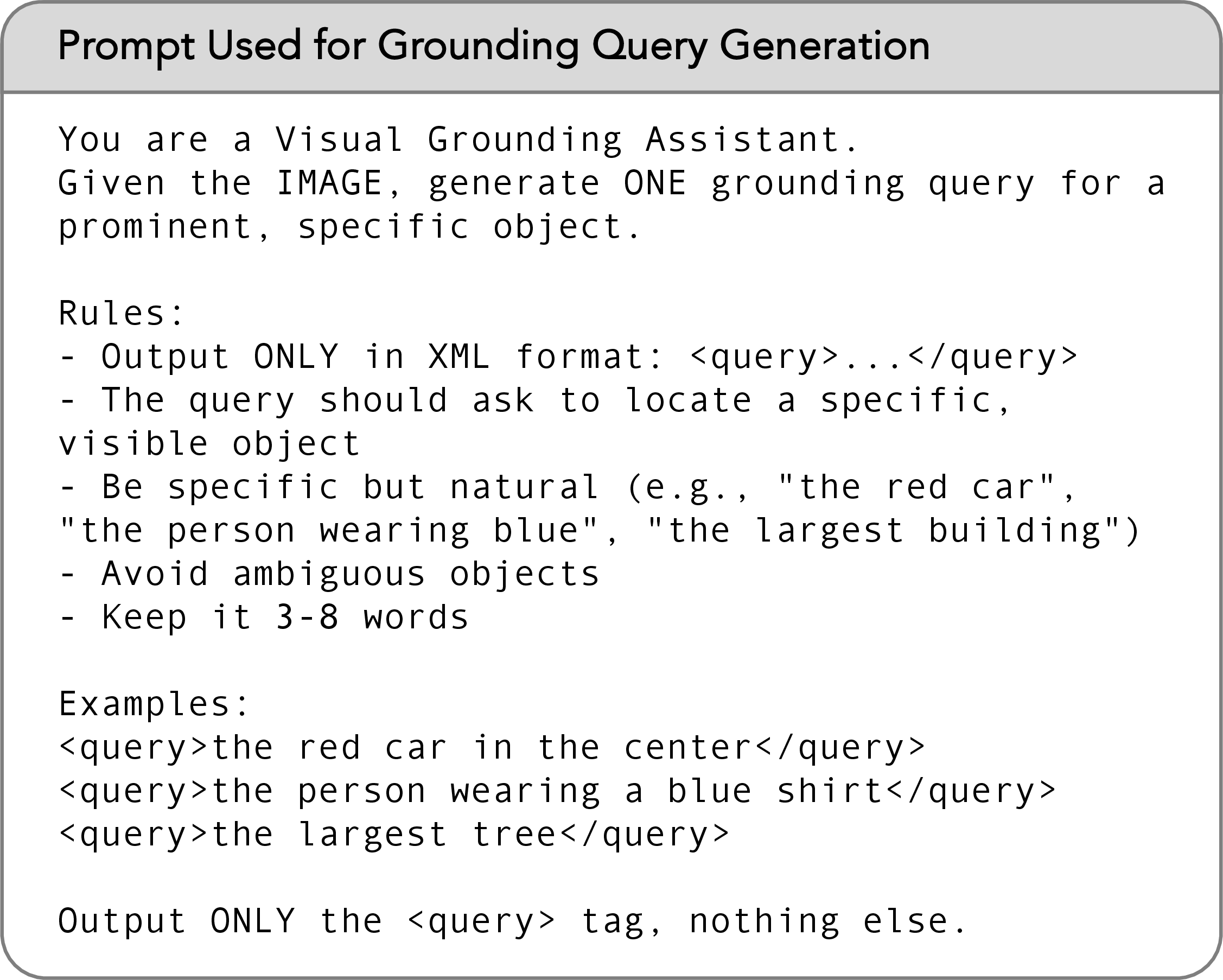
Figure 6: Prompts used at each stage of VISE training. (a) Grounding query generation. (b) Bounding box prediction. (c) Semantic visibility verification..
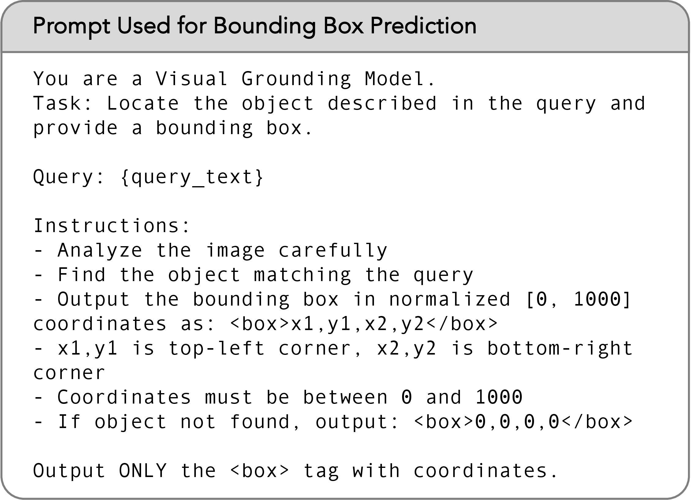
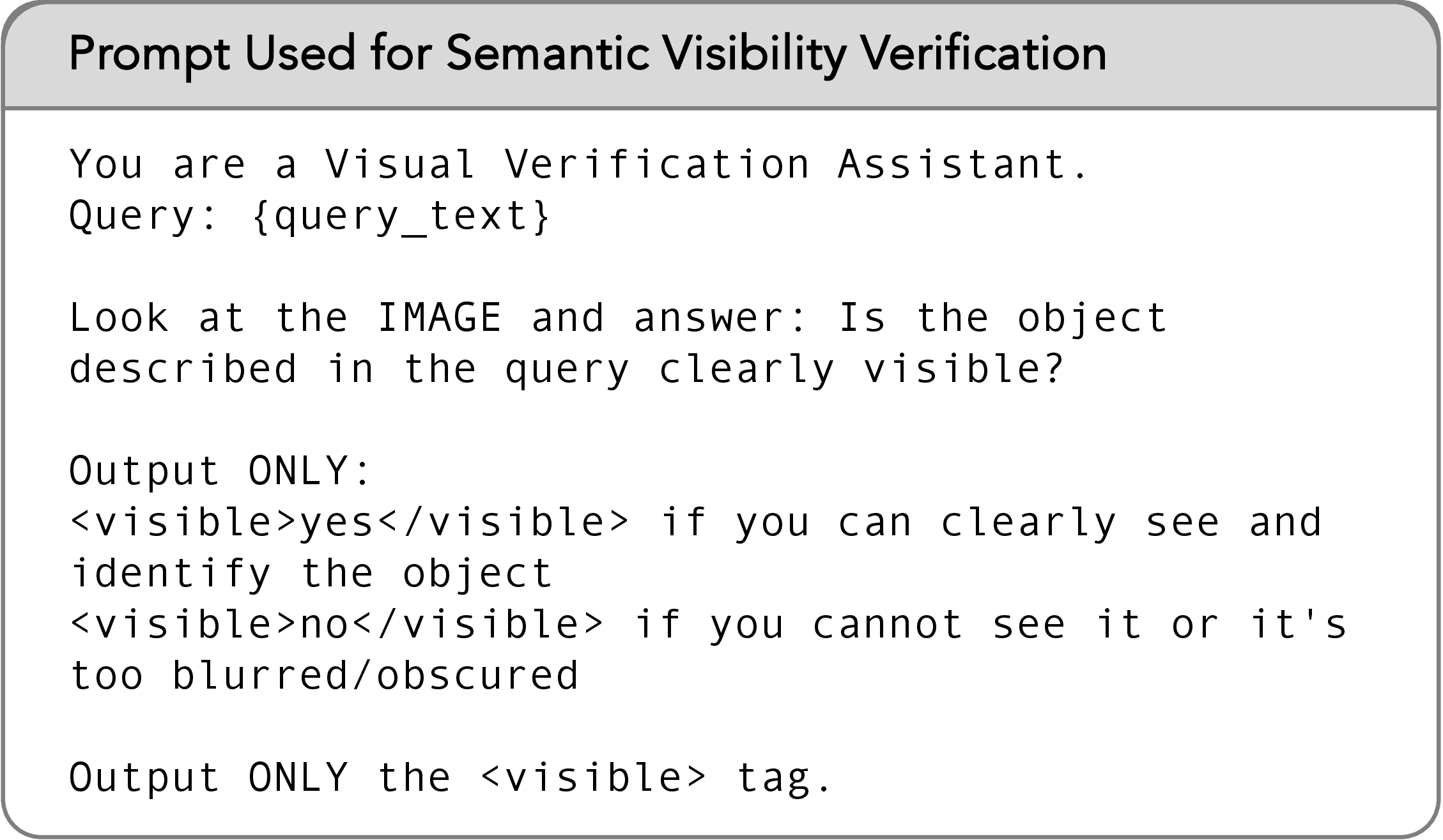
VISE uses three distinct prompts at each training step, one for each stage of the self-supervised pipeline. We describe each below and provide the corresponding prompt in the figures that follow.
At the start of each training step, the model is prompted to generate a natural-language grounding query \(q\) for the input image \(x\). The prompt instructs the model to identify a
single prominent, spatially unambiguous object in the scene and describe it concisely. The generated query is then used as input for both the bounding box prediction and the semantic visibility verification stages within the same step. No external query
bank, template, or category list is used — the query is produced entirely by the model itself from the raw image.
Given the image \(x\) (or its geometrically transformed version \(x' = \mathcal{T}(x)\)) and the generated query \(q\), the model is prompted to
predict a bounding box localizing the queried object. The prompt specifies the normalized coordinate space \([0, 1000]^4\) and the expected output format. This same prompt structure is used for both the original and
transformed views, ensuring that any difference in predicted boxes reflects the model’s visual grounding behavior rather than prompt variation.
9.3 Prompt Used for Semantic Visibility Verification↩︎
After predicting \(B_\text{orig}\), the model is prompted to assess whether the queried object is clearly visible in both the original image \(x\) and the ghosted image \(\tilde{x}\). The prompt asks for a binary yes/no judgment and is kept deliberately minimal to avoid leading the model toward a particular answer. The semantic invariance reward \(\mathcal{R}_\text{sem}\) is computed from the pair of visibility judgments returned by this prompt, as described in the Method Section of the main paper.
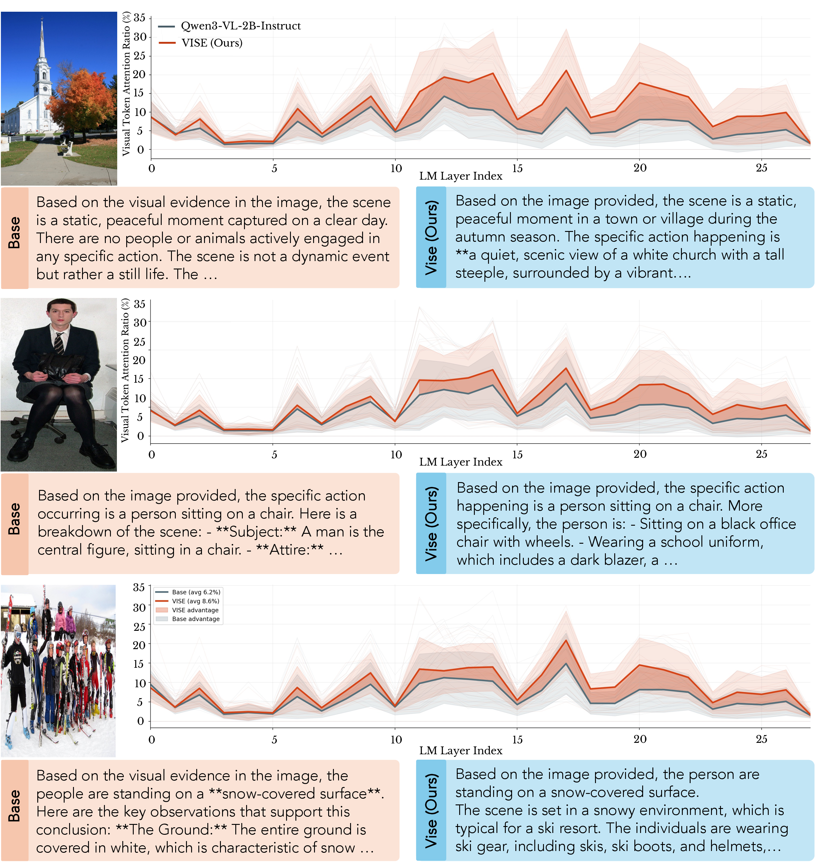
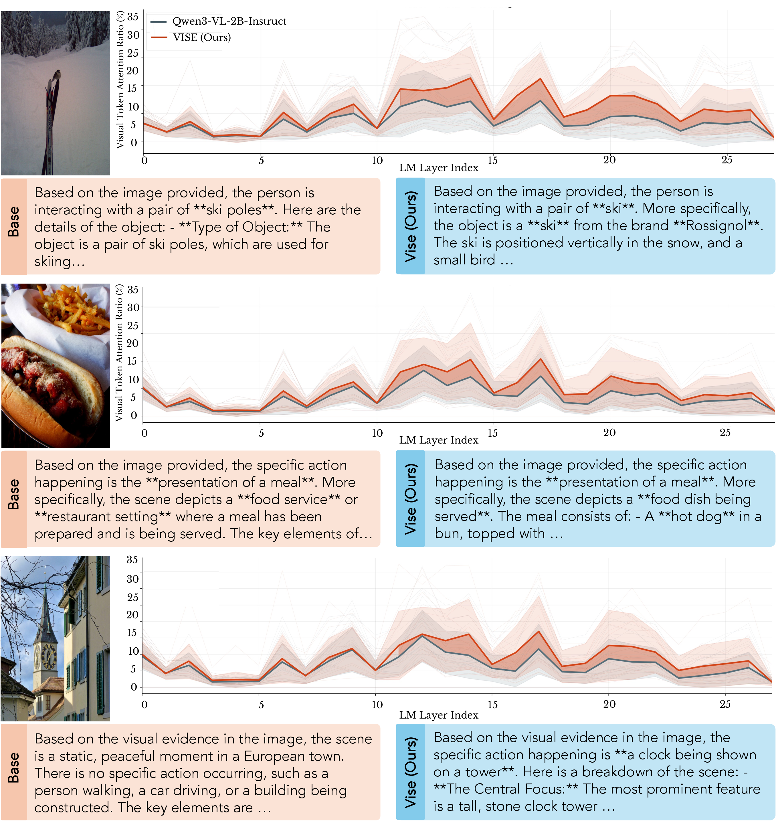
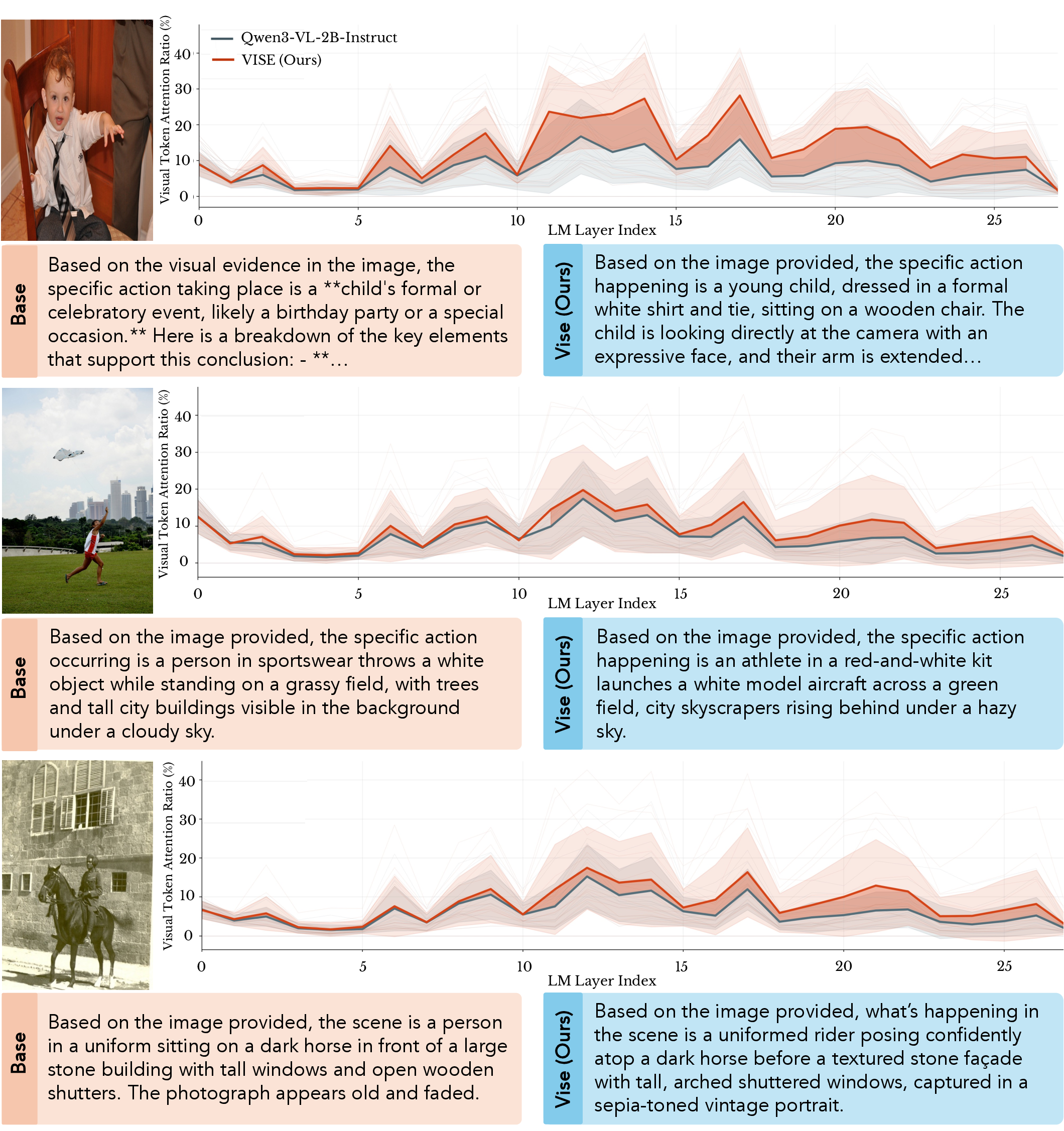
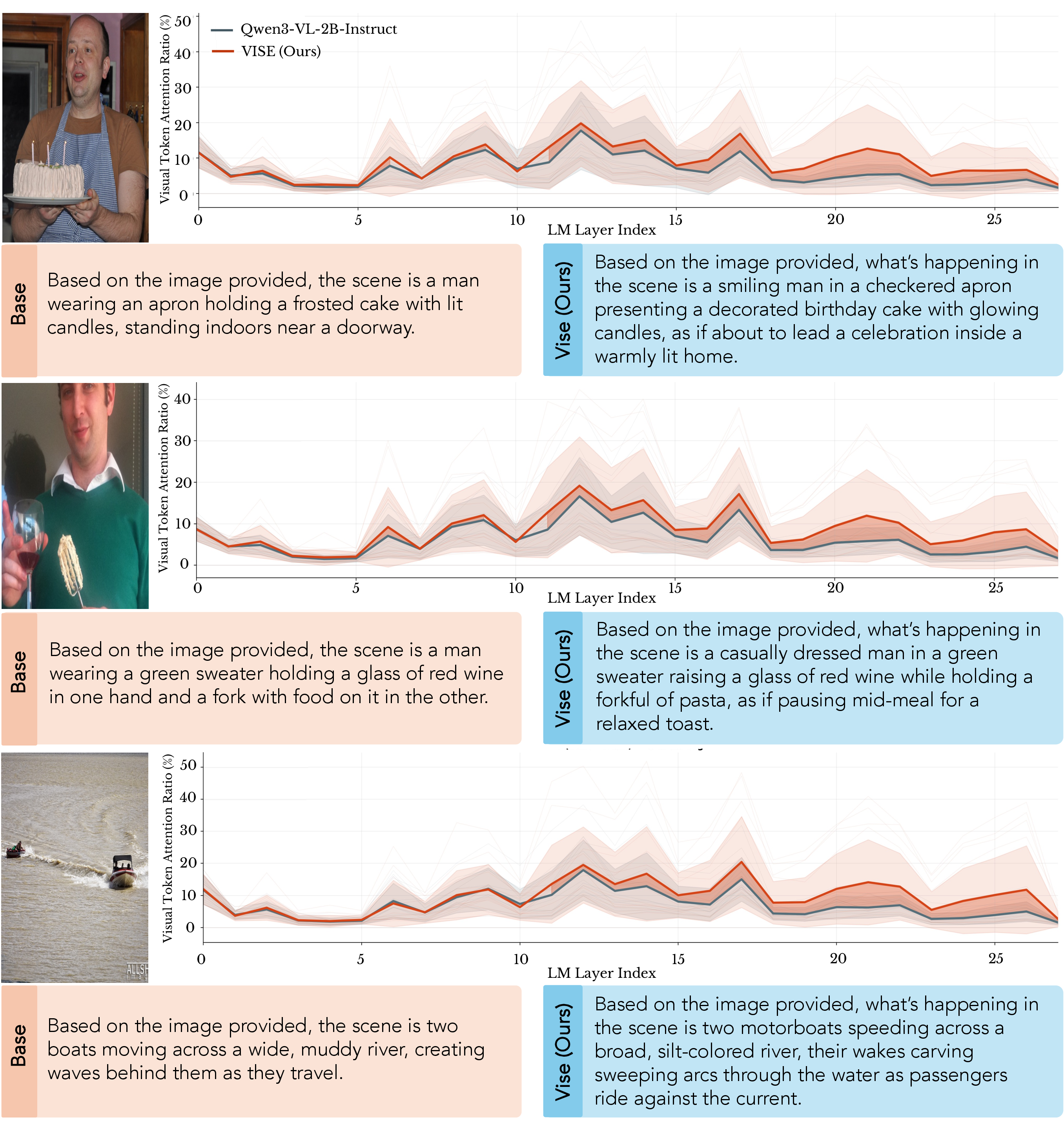
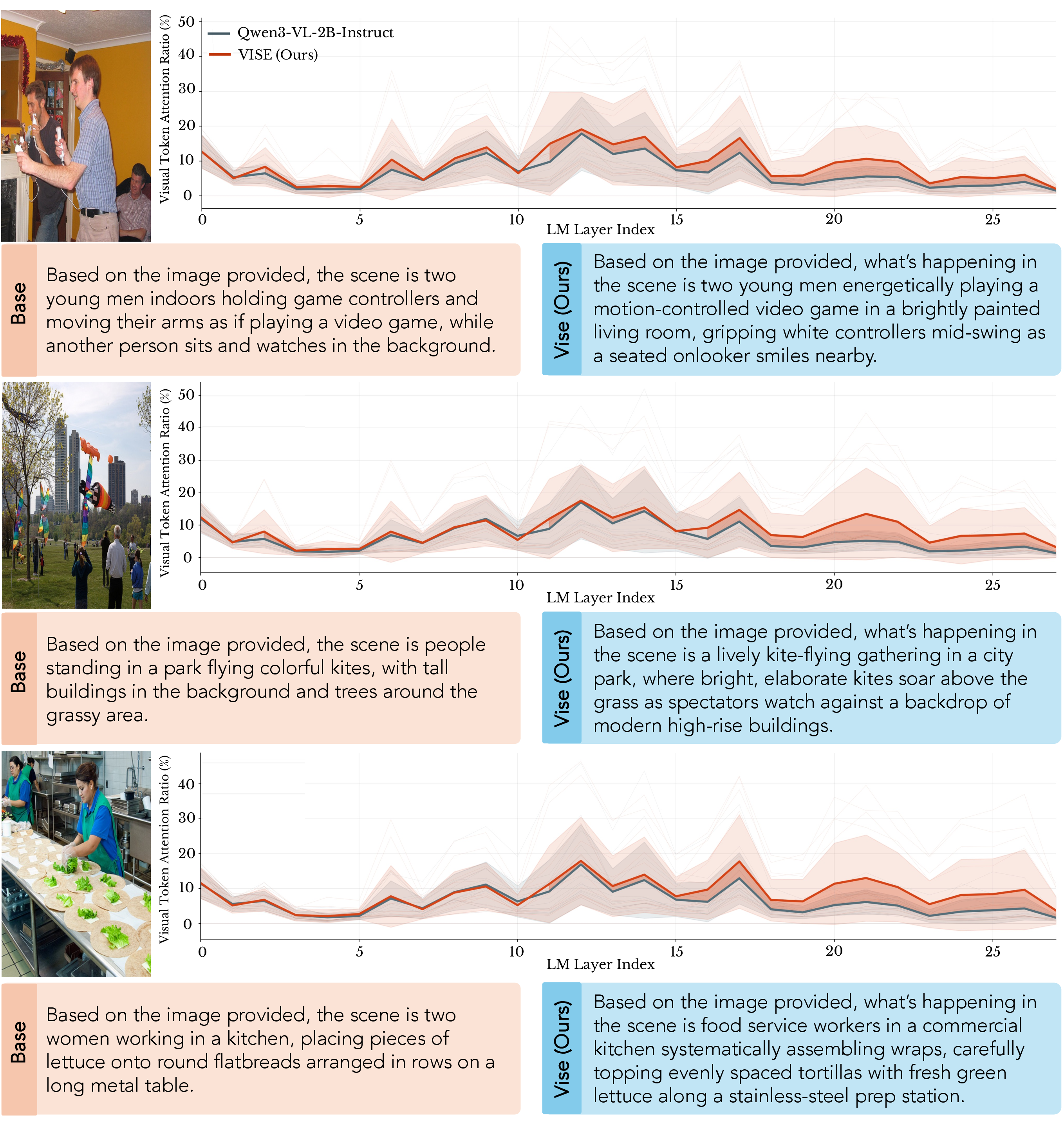
Figures 7–11 show additional per-sample, generation-time visual attention comparisons between the base Qwen3-VL-2B model [11] and VISE across a range of scene types using the prompt, "What is happening in this scene?" For each example, we plot the fraction
of attention allocated to image tokens at each decoder layer during generation, alongside the corresponding text outputs from both models. The attention advantage of VISE is consistent across all examples shown, concentrating in the mid-to-late decoder
layers where semantic generation decisions are made, and is accompanied by noticeably more specific and visually grounded output text.
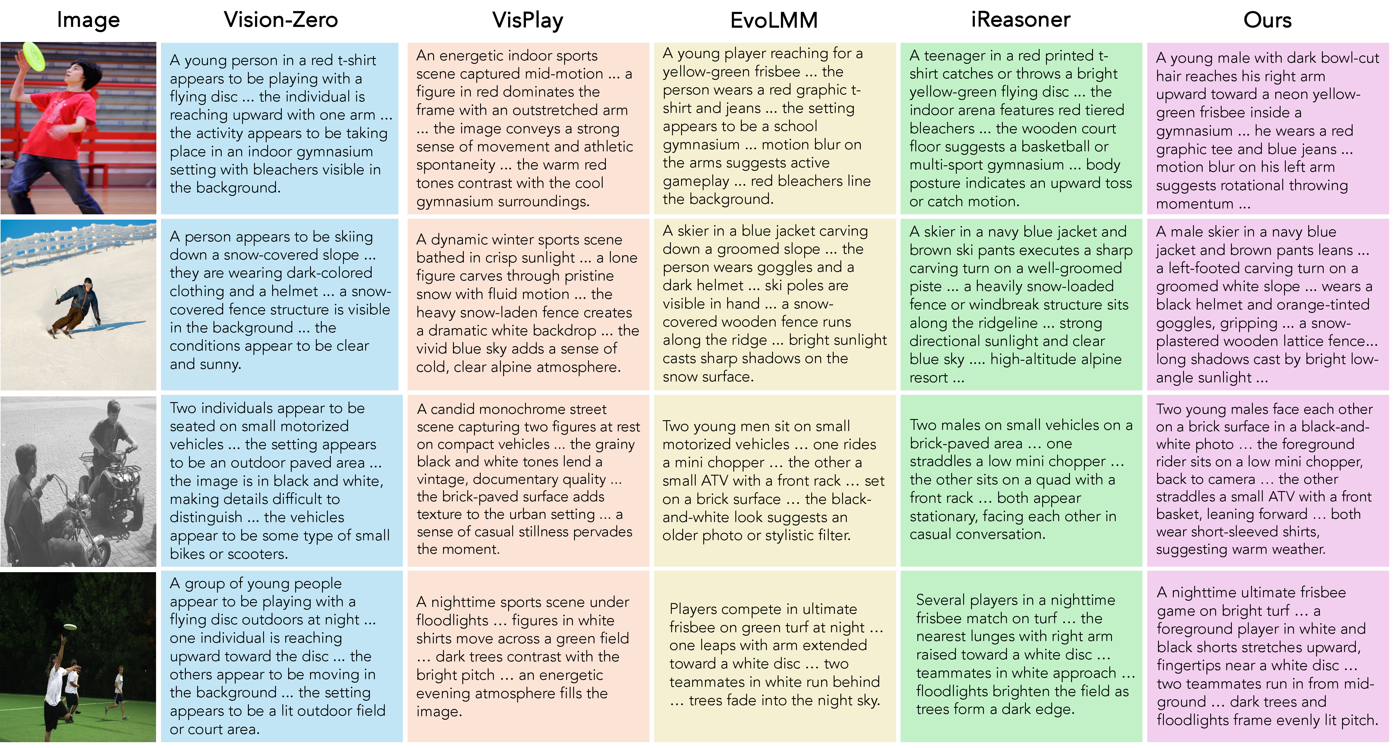
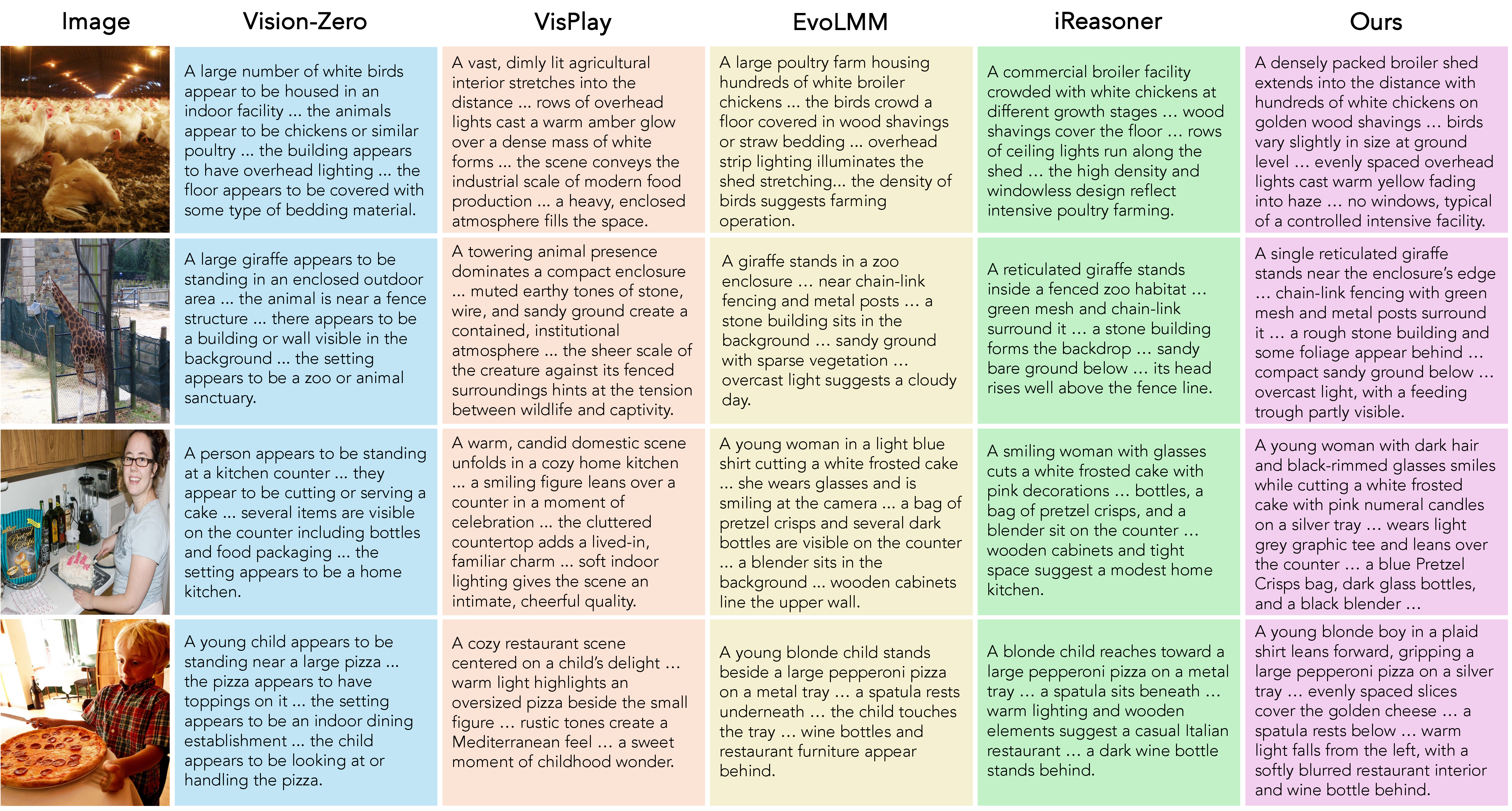
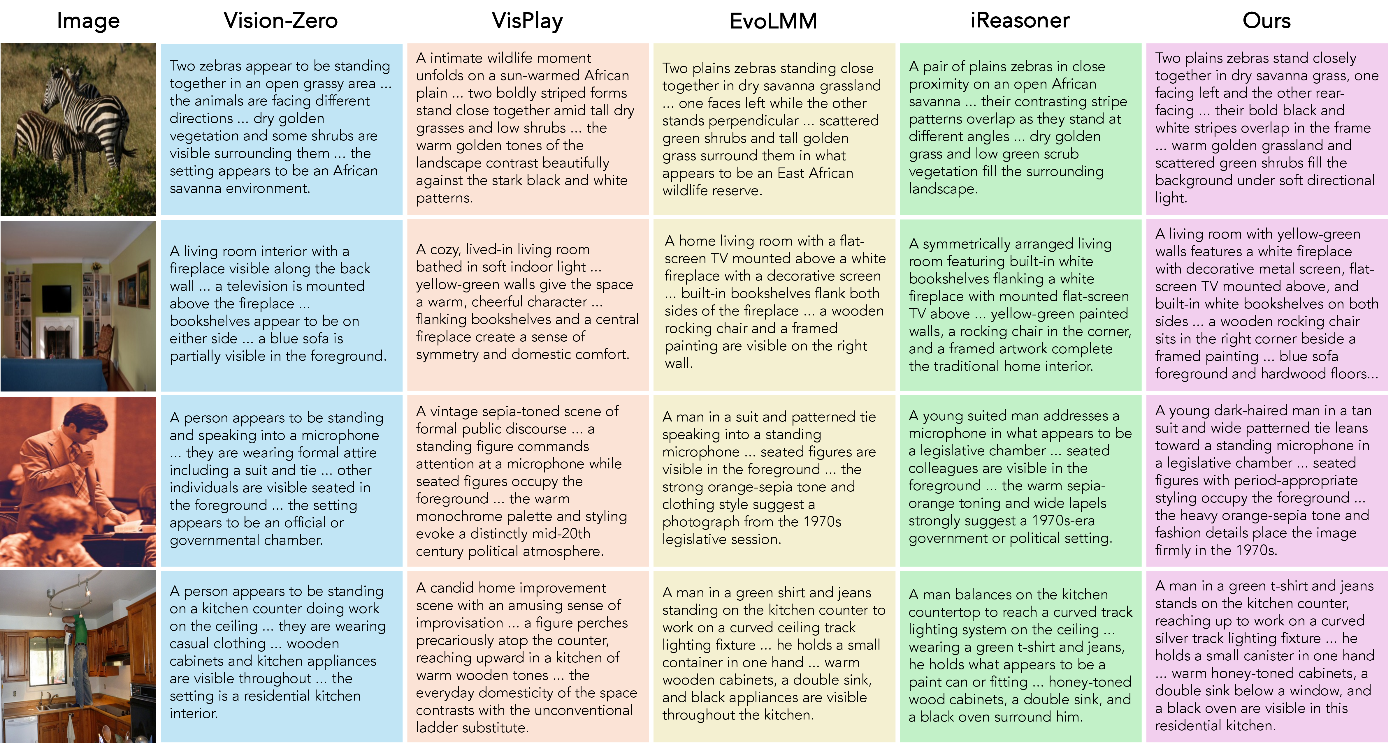
Figures 12 to 15 provide additional qualitative comparisons of image descriptions produced by VISE and four self-evolving baselines: VisionZero (RealWorld) [4], VisPlay [2], EvoLMM [1], and iReasoner [3]. All methods are evaluated on the same images under the same prompts using their respective Qwen3-VL-2B
checkpoints. Baseline methods tend to produce descriptions that are either vague and category-level, relying on statistically common scene descriptions, or occasionally confident but incorrect about specific visual details. VISE consistently produces more
fine-grained and accurate descriptions, correctly identifying object-level details such as clothing attributes, vehicle types, spatial relationships, and scene-specific context that the baselines miss or misattribute.
Figure 7: Additional generation-time visual attention comparisons between the base model and VISE on Qwen3-VL-2B. For each example, the attention plot shows the fraction of attention allocated to image tokens per decoder
layer, alongside the corresponding outputs from both models. VISE consistently attends more to visual tokens across mid-to-late layers, producing more grounded and specific descriptions.Figure 8: Additional generation-time visual attention comparisons (continued).Figure 9: Additional generation-time visual attention comparisons (continued).Figure 10: Additional generation-time visual attention comparisons (continued).Figure 11: Additional generation-time visual attention comparisons (continued).Figure 12: Additional qualitative comparisons of VISE against all baselines across diverse scene types. VISE consistently produces more specific and visually grounded descriptions, correctly identifying fine-grained details
such as clothing, object types, and spatial relationships that baselines either miss or describe only at a category level.Figure 13: Additional qualitative comparisons (continued).Figure 14: Additional qualitative comparisons (continued).Figure 15: Additional qualitative comparisons (continued).
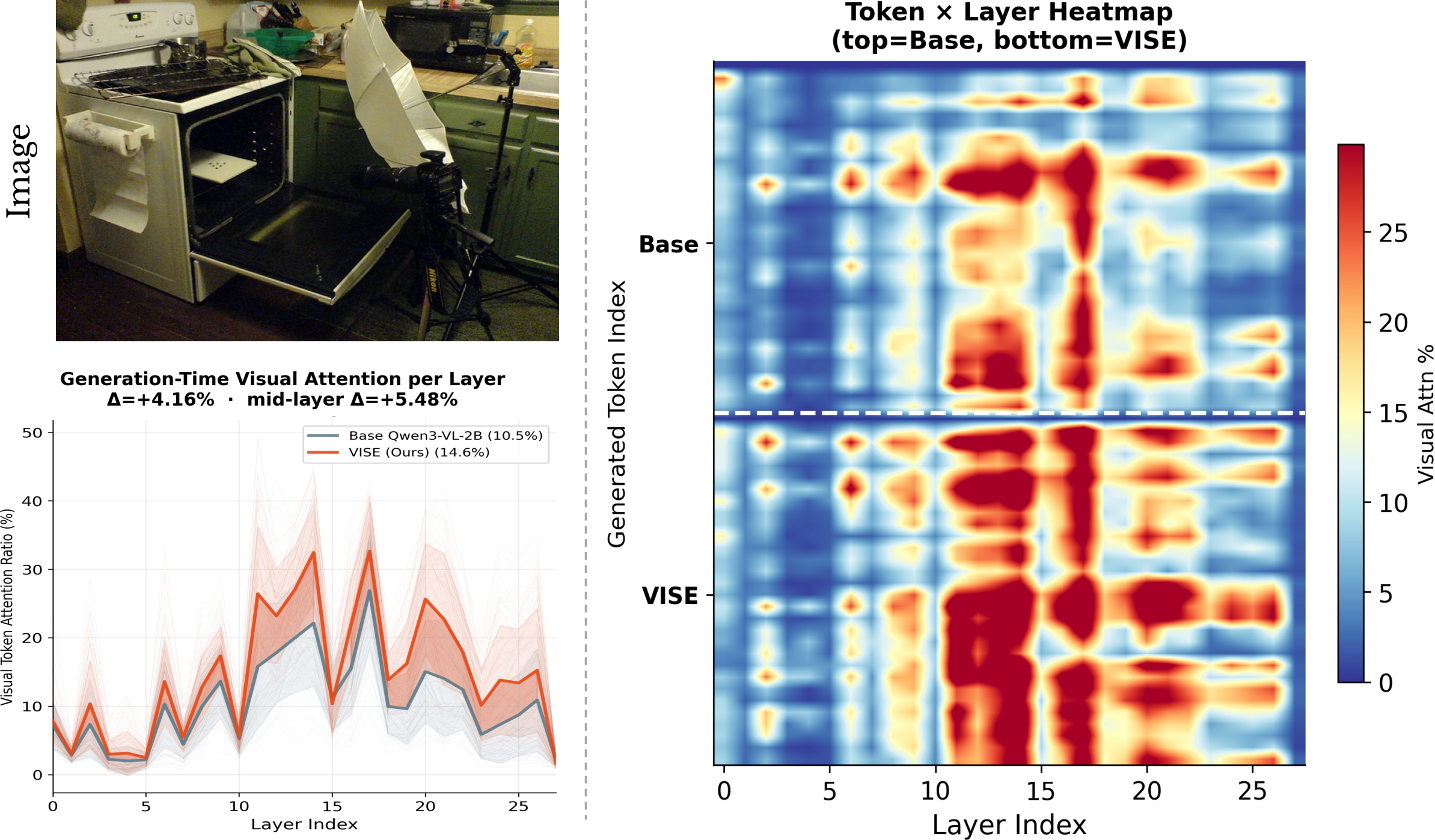
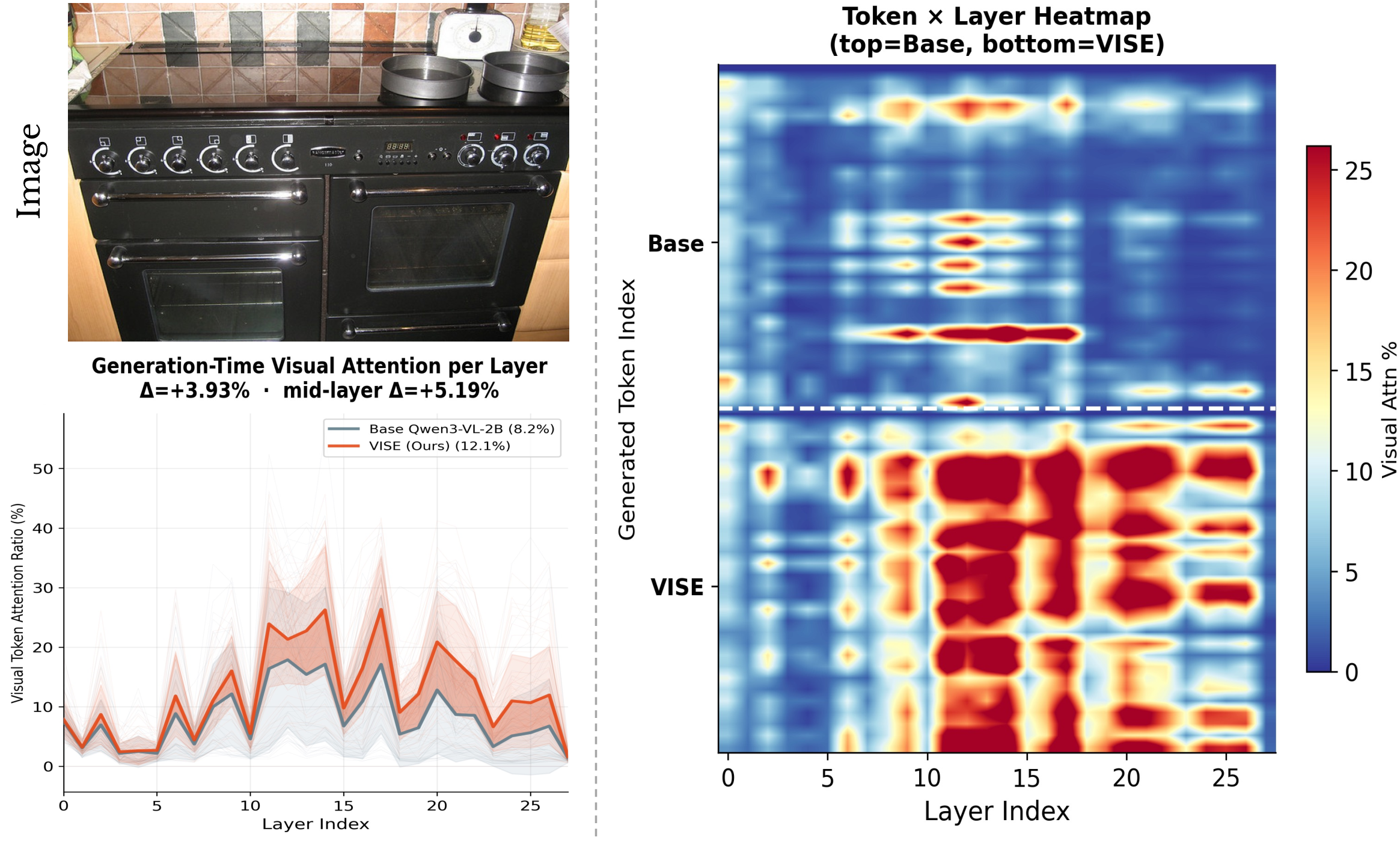
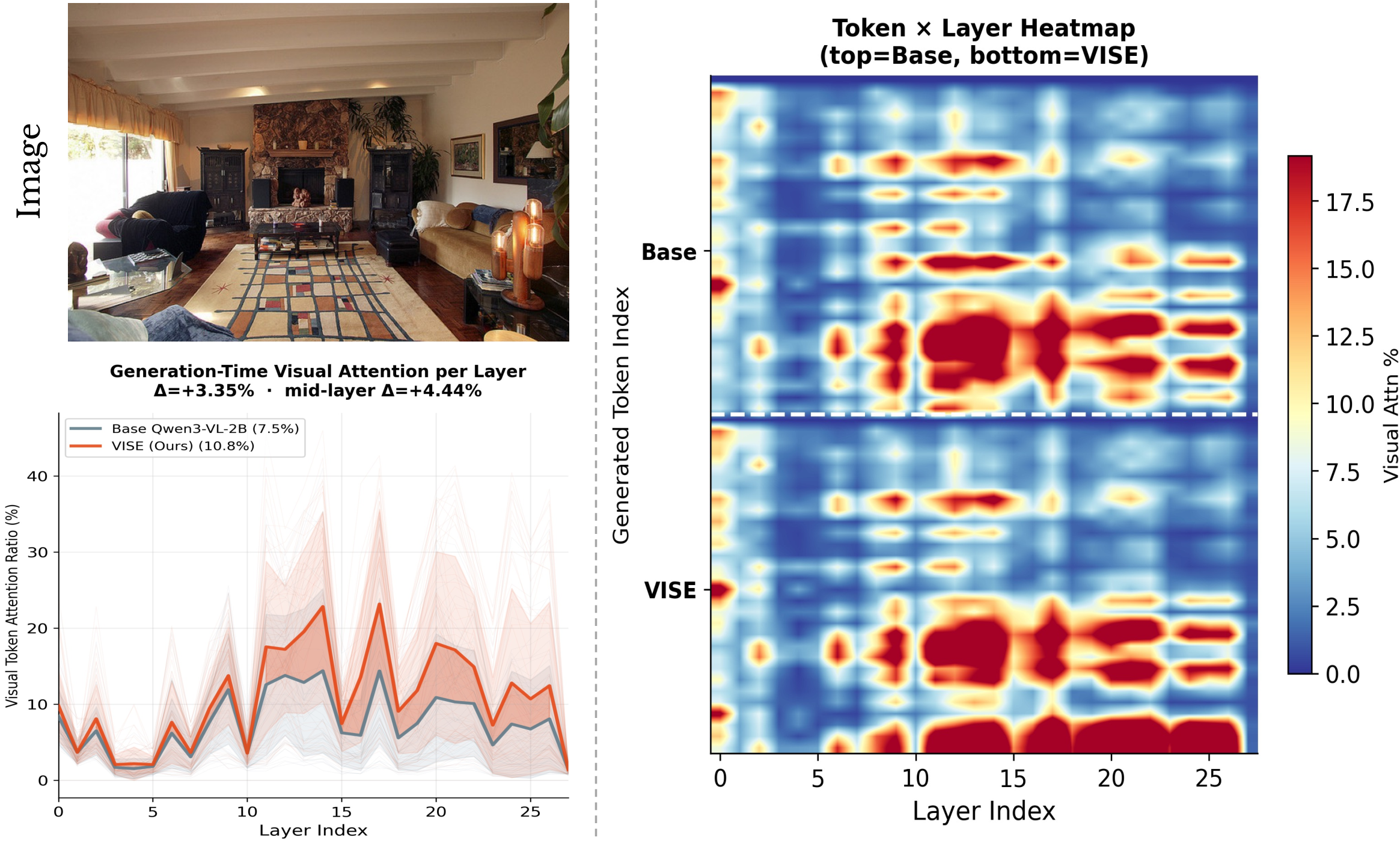
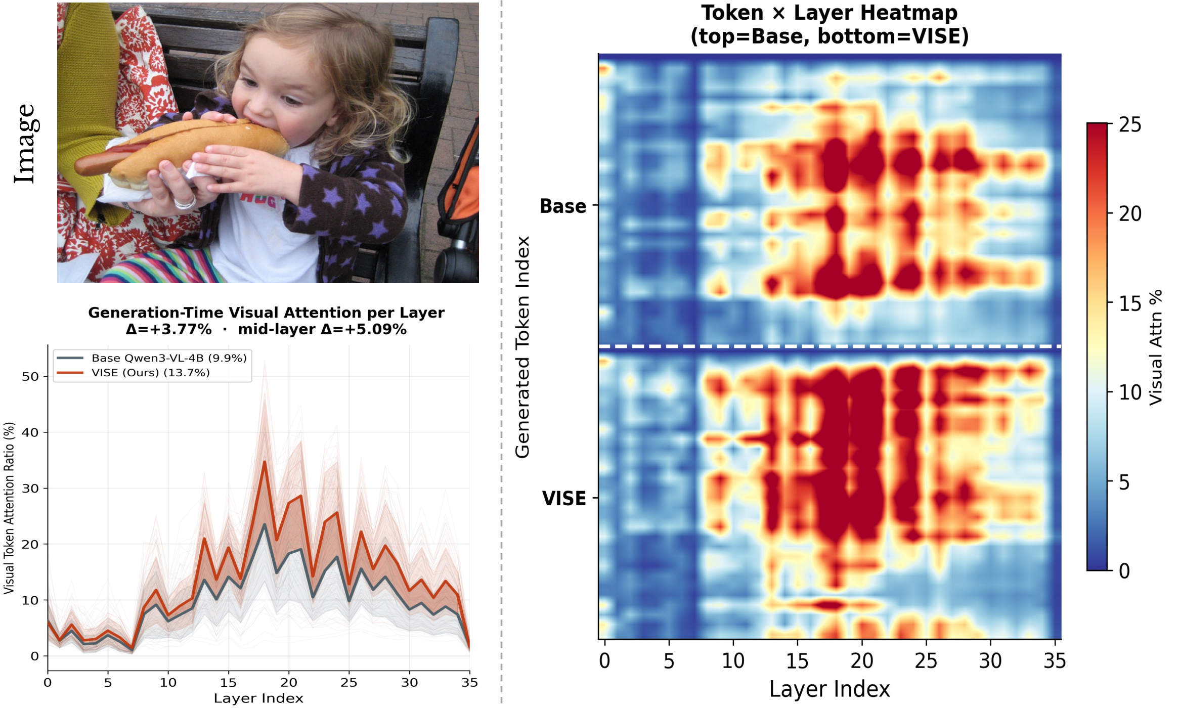
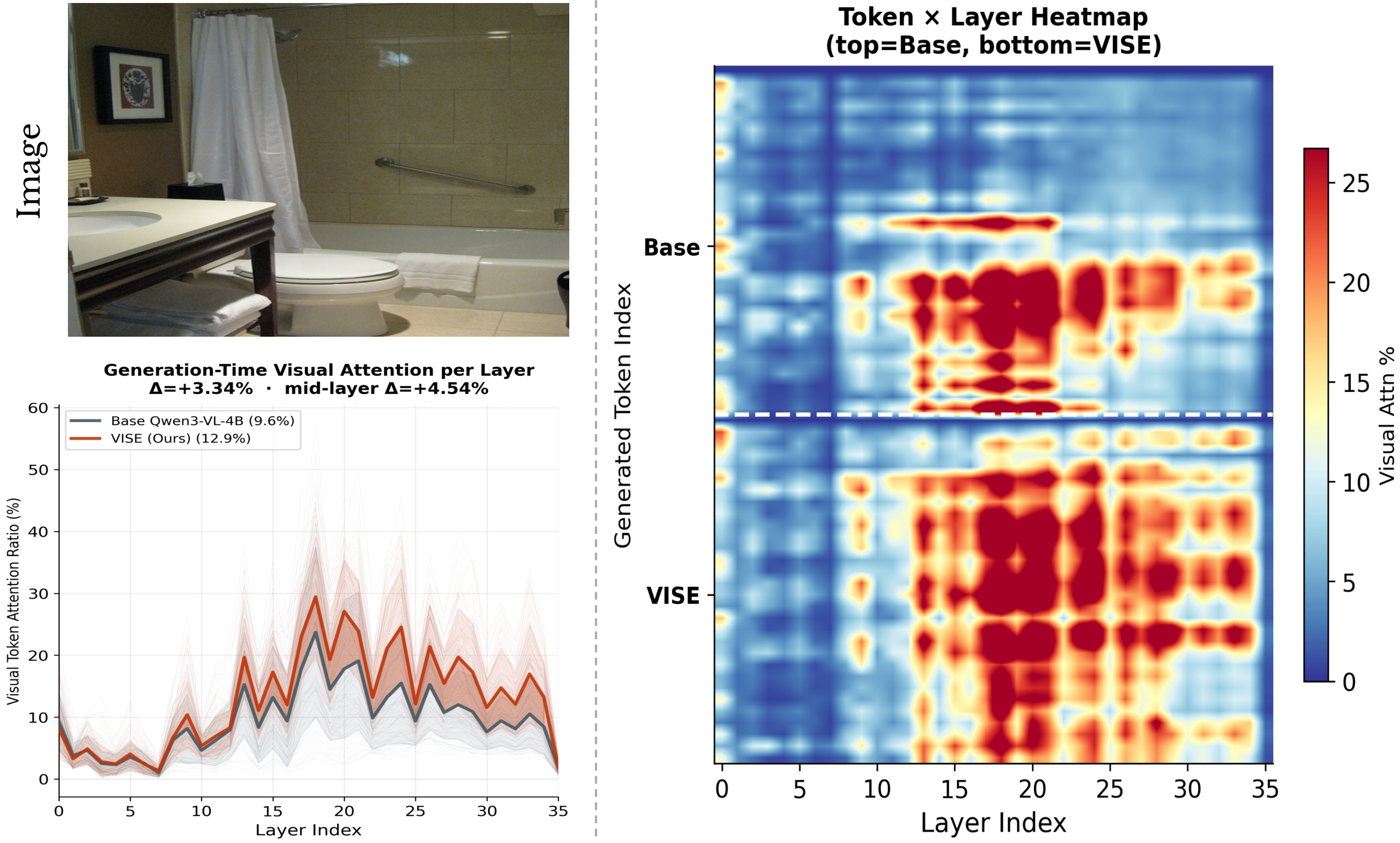
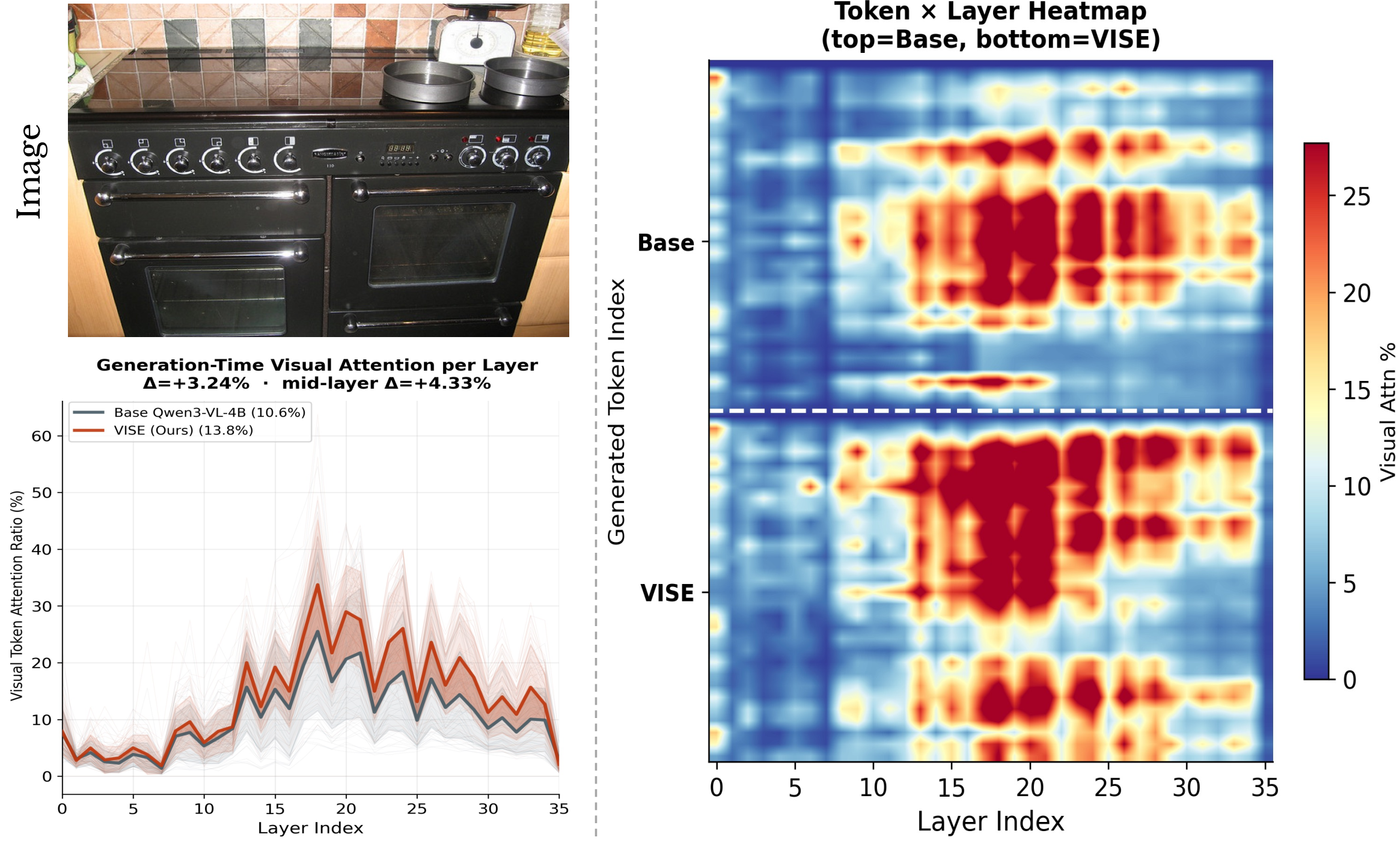
Figures 16–18 and Figures 19–21 show per-sample generation-time attention breakdowns for randomly selected
samples from the COCO dataset, evaluated on Qwen3-VL-2B and Qwen3-VL-4B respectively. Each figure shows the input image, a per-layer line plot of the visual token attention ratio during generation, and a Token\(\times\)Layer heatmap comparing the base model (top) and VISE (bottom) side by side. The line plots show that VISE consistently allocates a higher fraction of attention to image tokens throughout generation, with the advantage
most pronounced in mid-to-late layers where semantic content is produced. The heatmaps make this difference concrete at the token level: VISE shows broader and more intense red regions across both the layer and token axes, indicating that individual
generated tokens are more strongly anchored to visual evidence. This pattern holds across all six samples and both model scales, and is particularly strong in cases requiring spatial layout description and fine-grained visual detail. All samples are
evaluated using the prompt: “Describe in detail the spatial layout and positions of all objects in this image.”
Figure 16: Per-sample generation-time attention breakdown on Qwen3-VL-2B. Left: input image and per-layer visual token attention ratio for the base model and VISE. Right: Token\(\times\)Layer heatmap with base model (top) and VISE (bottom); red regions indicate high visual attention.Figure 17: Per-sample generation-time attention breakdown on Qwen3-VL-2B (sample 2).Figure 18: Per-sample generation-time attention breakdown on Qwen3-VL-2B (sample 3).Figure 19: Per-sample generation-time attention breakdown on Qwen3-VL-4B. The attention advantage concentrates in layers 15–25, consistent with the aggregate result in Figure 6 of the main paper.Figure 20: Per-sample generation-time attention breakdown on Qwen3-VL-4B (sample 2).Figure 21: Per-sample generation-time attention breakdown on Qwen3-VL-4B (sample 3).
O. Thawakar et al., arXiv preprint arXiv:2511.16672, 2025.
[2]
Y. He, C. Huang, Z. Li, J. Huang, and booktitle=Proceedings. of the I. C. on C. V. and P. R. Yang Yonghui, “VisPlay: Self-evolving vision-language models,” 2026, pp.
26274–26284.
[3]
M. Sunil, M. Venmathimaran, and M. S. Kavitha, arXiv preprint arXiv:2601.05877, 2026.
J. Liu et al., arXiv preprint arXiv:2511.19900, 2025.
[6]
A. Singh et al., “Beyond human data: Scaling self-training for problem-solving with language models,”arXiv preprint arXiv:2312.06585, 2023.
[7]
X. Wang et al., “Enhancing visual-language modality alignment in large vision language models via self-improvement,” 2025, pp. 268–282.
[8]
W. Liu, J. Li, X. Zhang, F. Zhou, Y. Cheng, and J. He, arXiv preprint arXiv:2412.17451, 2024.
[9]
X. Chen et al., arXiv preprint arXiv:2507.16518, 2025.
[10]
T. Li, Z. Sun, J. Wei, C. He, L. Wu, and booktitle=Proceedings. of the I. C. on C. V. and P. R. Tan Cheng, “Decouple to generalize: Context-first self-evolving learning for
data-scarce vision-language reasoning,” 2026, pp. 29357–29366.
[11]
S. Bai et al., “Qwen3-VL technical report.” 2025 , eprint={2511.21631}, archivePrefix={arXiv}, primaryClass={cs.CV}, [Online]. Available: https://arxiv.org/abs/2511.21631.
[12]
H. Rezatofighi, N. Tsoi, J. Gwak, A. Sadeghian, I. Reid, and booktitle=Proceedings. of the I. conference on computer vision and pattern recognition Savarese Silvio, “Generalized
intersection over union: A metric and a loss for bounding box regression,” 2019, pp. 658–666.
[13]
S. Kornblith, M. Norouzi, H. Lee, and booktitle=International. C. on M. L. Hinton Geoffrey, “Similarity of neural network representations revisited,” 2019 ,
organization={PMLR}, pp. 3519–3529.
I. Loshchilov and F. Hutter, “Decoupled weight decay regularization,”arXiv preprint arXiv:1711.05101, 2017.
[16]
T.-Y. Lin et al., “Microsoft coco: Common objects in context,” 2014 , organization={Springer}, pp. 740–755.
[17]
K. Zhang et al., “Lmms-eval: Reality check on the evaluation of large multimodal models,” 2025, pp. 881–916.
[18]
H. Agrawal et al., “Nocaps: Novel object captioning at scale,” 2019, pp. 8948–8957.
[19]
B. A. Plummer, L. Wang, C. M. Cervantes, J. C. Caicedo, J. Hockenmaier, and booktitle=Proceedings. of the I. international conference on computer vision Lazebnik Svetlana,
“Flickr30k entities: Collecting region-to-phrase correspondences for richer image-to-sentence models,” 2015, pp. 2641–2649.
[20]
O. Sidorov, R. Hu, M. Rohrbach, and booktitle=European. conference on computer vision Singh Amanpreet, “Textcaps: A dataset for image captioning with reading comprehension,”
2020 , organization={Springer}, pp. 742–758.
[21]
D. A. Hudson and booktitle=Proceedings. of the I. conference on computer vision and pattern recognition Manning Christopher D, “Gqa: A new dataset for real-world visual reasoning
and compositional question answering,” 2019, pp. 6700–6709.
[22]
K. Marino, M. Rastegari, A. Farhadi, and booktitle=Proceedings. of the I. conference on computer vision and pattern recognition Mottaghi Roozbeh, “Ok-vqa: A visual question
answering benchmark requiring external knowledge,” 2019, pp. 3195–3204.
[23]
Y. Goyal, T. Khot, D. Summers-Stay, D. Batra, and booktitle=Proceedings. of the I. conference on computer vision and pattern recognition Parikh Devi, “Making the v in vqa matter:
Elevating the role of image understanding in visual question answering,” 2017, pp. 6904–6913.
[24]
A. Kembhavi, M. Salvato, E. Kolve, M. Seo, H. Hajishirzi, and booktitle=European. conference on computer vision Farhadi Ali, “A diagram is worth a dozen images,” 2016 ,
organization={Springer}, pp. 235–251.
[25]
A. Masry, J. Q. Tan, S. Joty, E. Hoque, and booktitle=Findings. of the association for computational linguistics:. A. 2022. others, “Chartqa: A benchmark for question answering
about charts with visual and logical reasoning,” 2022, pp. 2263–2279.
[26]
M. Mathew, V. Bagal, R. Tito, D. Karatzas, E. Valveny, and booktitle=Proceedings. of the I. W. C. on A. of C. V. Jawahar CV, “Infographicvqa,” 2022, pp. 1697–1706.
[27]
P. Lu et al., “Learn to explain: Multimodal reasoning via thought chains for science question answering,”Advances in neural information processing
systems, vol. 35, pp. 2507–2521, 2022.
[28]
X. Yue et al., “Mmmu: A massive multi-discipline multimodal understanding and reasoning benchmark for expert agi,” 2024, pp. 9556–9567.
[29]
S. Yang et al., “Captionqa: Is your caption as useful as the image itself?” 2026, pp. 23741–23750.
M. Du, B. Wu, Z. Li, X.-J. Huang, and booktitle=Proceedings. of the 62nd. A. M. of the A. for C. L. (. Wei Zhongyu, “Embspatial-bench: Benchmarking spatial understanding for
embodied tasks with large vision-language models,” 2024, vol. 2: Short Papers), pp. 346–355.
[32]
Y. Liu et al., “Mmbench: Is your multi-modal model an all-around player?” 2024 , organization={Springer}, pp. 216–233.
[33]
Y. Li, Y. Du, K. Zhou, J. Wang, X. Zhao, and booktitle=Proceedings. of the 2023. conference on empirical methods in natural language processing Wen Ji-Rong, “Evaluating object
hallucination in large vision-language models,” 2023, pp. 292–305.
[34]
A. Rohrbach et al., “Object hallucination in image captioning,” 2018", address = "Brussels, Belgium, pp. 4035–4045, doi: 10.18653/v1/D18-1437.

![Figure 1: Overview of VISE compared to prior self-evolving methods. [1]–[4] (Left) Prior approaches use separate roles with role-specific objectives optimized for answer consistency, whereas our VISE operates within a single model using geometric and semantic invariance rewards. (Right) For chart-based queries that require minimal visual dependence, both the prior method and our VISE provide accurate answers. However, on real-scene understanding tasks that require deeper visual semantics, prior approaches struggle, likely because the language decoder resorts to statistically plausible scenarios (a “ramp surface” instead of a “metal ledge”). In contrast, VISE accurately identifies the metal ledge, likely due to learning self-consistent visual invariance during unsupervised training. Additional examples are provided in the suppl. material.](/article/2606.27373/assets/Teaser.png "fig:")