Beyond the Hard Budget: Sparsity Regularizers for More Interpretable Top-k Sparse Autoencoders
June 25, 2026
Abstract
Sparse autoencoders (SAEs) have become a leading tool for interpreting the representations of vision foundation models, decomposing their polysemantic activations into a larger set of sparse, more monosemantic features. The Top-\(k\) SAE, a now-standard variant, enforces sparsity architecturally through its activation function, retaining only the \(k\) most active latents per input. Because it was designed precisely to avoid the \(\ell_1\) penalty used by earlier SAEs and its known drawbacks, it has not been combined with an explicit sparsity regularizer–despite retaining limitations of its own, such as a budget \(k\) that is fixed regardless of input complexity and a tendency to overfit to the training value of \(k\). We introduce two sparsity regularizers compatible with the Top-\(k\) architecture, both acting on the activations before the Top-\(k\) selection: an \(\ell_1\) penalty on the unselected (off-support) units, and a scale-invariant \(\ell_1/\ell_2\)-ratio penalty that concentrates the code onto fewer effective units. Both penalties are applied only to the batch-active units, those selected by the Top-\(k\) operator at least once within the batch. Across two datasets, three vision foundation models, and a range of \(k\), both regularizers consistently improve monosemanticity at no cost to reconstruction quality. The \(\ell_1/\ell_2\) penalty further concentrates information into fewer latents, making reconstruction more robust to the inference-time choice of \(k\) and improving small-budget linear probing. Our central finding is that hard architectural sparsity and soft sparsity regularization are complementary rather than mutually exclusive.
1 1 Introduction↩︎
Vision foundation models (VFMs) have become a standard source of general-purpose image embeddings. Yet the embeddings they produce are difficult to interpret, in part because of the polysemanticity: a single coordinate of the representation may respond to many seemingly unrelated concepts. A leading explanation for this phenomenon is superposition, whereby a network represents more features than it has dimensions by encoding them as overlapping, non-orthogonal vectors [1]. This opacity is an obstacle to auditing and controlling systems built on top of these models.
Sparse autoencoders (SAEs) have recently emerged as a promising tool for interpreting such representations. An SAE encodes an input embedding into a higher-dimensional latent space under a sparsity constraint and reconstructs the input from this sparse code, with the aim of recovering latent units that are as monosemantic as possible, ideally, each responding to a single human-interpretable concept. Initially used to interpret the internal activations of large language models (LLMs) [2], [3], SAEs have since been applied to the embeddings of vision foundation models, where they are used to extract and study interpretable visual features [4]–[6].
SAEs differ in how they impose sparsity. The original formulation, which we refer to as the vanilla SAE, adds an explicit \(\ell_1\) penalty on the latent code to the reconstruction loss. Because this penalty grows with activation magnitude, it biases the encoder toward systematically reducing the magnitudes of active units–a phenomenon known as feature shrinkage [7], [8]–and vanilla SAE training is in general prone to producing dead latents, units that cease to activate entirely [7]. The Top-\(k\) SAE [7], building on the \(k\)-sparse autoencoder [9], was introduced specifically to dispense with the \(\ell_1\) penalty: it imposes sparsity architecturally, through an activation function that retains, for each input, only the \(k\) latent units with the largest activations and zeroes the rest. This enforces a hard per-sample sparsity budget while avoiding the magnitude shrinkage induced by the \(\ell_1\) term.
Perhaps because the Top-\(k\) SAE was conceived precisely to remove the \(\ell_1\) penalty, the literature has not revisited augmenting it with an additional sparsity constraint acting on the latent code. Yet the Top-\(k\) SAE retains its own well-documented limitations, several of which an additional sparsity term could plausibly address. First, the sparsity level \(k\) is uniform across samples, even though the number of latent factors needed to describe an input is likely to vary with its complexity; this rigidity has motivated a line of work that relaxes the per-sample budget, for example by enforcing it only on average across a batch [10], by allocating it adaptively across units [11], or by predicting an input-dependent \(k\) [12], [13]. The standard objective, however, is indifferent to how many of the \(k\) available units are actually used, provided the reconstruction is accurate; it therefore gives the model no incentive to encode an easy sample with fewer than \(k\) units. A sparsity penalty acting on the activations before selection would supply precisely this missing incentive, letting the effective number of active units adapt to each input rather than remaining fixed at \(k\). Second, the value of \(k\) itself is chosen arbitrarily, and a Top-\(k\) SAE tends to overfit to its training \(k\), in the sense that its reconstruction quality degrades when the number of units retained at inference departs from the value used during training [7]. Encouraging the model to concentrate its reconstruction onto fewer units would reduce its reliance on the exact value of \(k\), and so mitigate this sensitivity.
To address these limitations, we introduce two sparsity regularizers compatible with the Top-\(k\) architecture. Both act on the activations before the Top-\(k\) selection and are restricted to the batch-active units: the units selected by the Top-\(k\) operator at least once within the batch. The first is an \(\ell_1\) penalty on the off-support activations–those of units not selected by the Top-\(k\) operator for a given sample. In a standard Top-\(k\) SAE these activations receive no gradient from the reconstruction objective and are therefore left unconstrained, allowing a unit to produce moderate, sub-threshold responses to inputs unrelated to the concept it encodes when selected. Penalizing them drives these off-support responses toward zero, sharpening each unit’s selectivity: a unit is encouraged to activate strongly only on the inputs for which it is among the top contributors and to remain near-zero otherwise. We show that this yields more coherent activating image sets and higher monosemanticity. The second regularizer penalizes the ratio of the \(\ell_1\) to the \(\ell_2\) norm of the activations, a scale-invariant sparsity measure introduced by [14]. Minimizing it concentrates the code onto fewer effective units; we show that this concentration directly mitigates several of the limitations above.
We evaluate on two datasets, ImageNet-1K [15] and Open Images V7 [16], using the embeddings of three frozen vision foundation models–CLIP [17], SigLIP2[18], and a supervised ViT-L/16 [19]—across a range of \(k\). We assess interpretability with the Monosemanticity Score of [6], a label-grounded class-purity measure, and qualitative inspection, and we study the downstream effects of the induced concentration. Across all configurations, the use of both regularizers yield markedly more concentrated and more interpretable codes without hurting reconstruction quality.
Our contributions are as follows:
We introduce two sparsity regularizers compatible with the Top-\(k\) architecture, both acting on the pre-selection activations: an off-support \(\ell_1\) penalty and an \(\ell_1/\ell_2\)-ratio penalty.
Across two datasets, three vision foundation models, and a range of \(k\), we show that both regularizers consistently improve interpretability–measured by monosemanticity and class purity–while preserving reconstruction quality.
We show that the concentration induced by the \(\ell_1/\ell_2\)-ratio regularizer addresses a known limitations of the Top-\(k\) SAE: it makes reconstruction substantially more robust to the inference-time choice of \(k\). Additionnally it concentrates discriminative information into fewer leading units, improving small-budget linear probing.
2 2 Related Work↩︎
2.0.0.1 Sparse autoencoders for vision.
Sparse autoencoders (SAEs) were originally introduced to interpret the internal activations of large language models (LLMs), decomposing them through dictionary learning into a larger set of sparse, more monosemantic latent units [2]. The same approach has since been transferred to the embeddings of vision foundation models (VFMs), where SAEs are used to extract and study human-interpretable visual features [4], [5]. We follow this line of work and train SAEs on the embeddings of frozen vision foundation models.
2.0.0.2 Monosemanticity.
A central goal of an SAE is to recover latent units that are as monosemantic as possible, that is, units each responding to a single human-interpretable concept. To quantify this property for vision SAEs, [6] introduce the Monosemanticity Score, which measures how similar the images that most strongly activate a given latent unit are to one another; higher values indicate a more concept-selective unit. We adopt the Monosemanticity Score as our primary measure of interpretability.
2.0.0.3 Top-\(k\) sparse autoencoders.
SAEs differ in how they impose sparsity. Early SAEs add an explicit \(\ell_1\) penalty on the latent code to the reconstruction loss which causes the suppression of weaker features [7], [8]. The Top-\(k\) sparse autoencoder [7] instead imposes sparsity architecturally, through its activation function: for each input it keeps only the \(k\) latent units with the largest activations and sets the remaining ones to zero. This enforces a hard per-sample sparsity budget and avoids the magnitude shrinkage caused by the \(\ell_1\) penalty. We build directly on this architecture.
2.0.0.4 Regularizing the Top-\(k\) sparse autoencoder.
In the Top-\(k\) sparse autoencoder, sparsity is controlled solely through the hard selection of the \(k\) largest activations. Prior attempts to add regularization in this setting act elsewhere than on the latent code: for instance, weight regularization penalizes the encoder and decoder weights, rather than the activations, to improve the stability of the learned features [20]. To the best of our knowledge, no prior work augments a Top-\(k\) sparse autoencoder with an explicit sparsity penalty applied directly to the activation vector seen by the Top-\(k\) operator. This is the gap addressed by the two regularizers we propose.
2.0.0.5 The \(\ell_1/\ell_2\) ratio as a sparsity measure.
One of our regularizers penalizes the ratio of the \(\ell_1\) to the \(\ell_2\) norm of the activations. This ratio originates from the sparseness measure of [14], defined as a normalized \(\ell_1/\ell_2\) ratio that is invariant to the scale of the vector. [21] subsequently proposed the Hoyer-Square regularizer, the squared \(\ell_1/\ell_2\) ratio, as a differentiable and scale-invariant surrogate for the \(\ell_0\) count, and used it to train sparser neural networks at comparable accuracy. Our second regularizer adapts this \(\ell_1/\ell_2\)-ratio family to the activations of a Top-\(k\) sparse autoencoder.
3 3 Method↩︎
Top-\(k\) sparse autoencoder enforces sparsity of its latent code only through its Top-\(k\) activation function[7].
We propose two regularizers compatible with the Top-\(k\) architecture, each imposing an additional sparsity constraint on the activations before the Top-\(k\) operator. Their effects are illustrated in Figure 1.
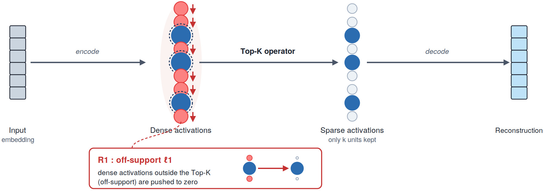
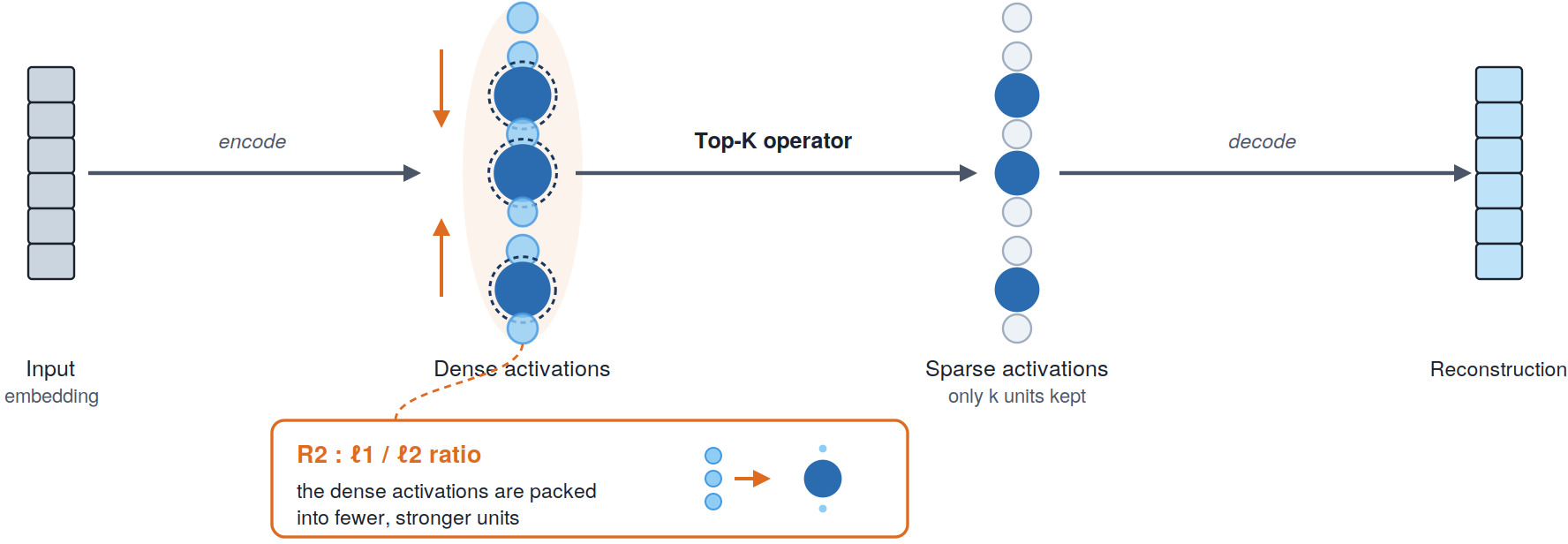
Figure 1: Effect of the two regularizers on the pre-selection activations. (left) Regularizer 1 shrinks the activations not selected by the Top-\(k\) operator toward \(0\); (right) Regularizer 2 concentrates the activation vector onto fewer units..
3.1 3.1 Notation and Architecture↩︎
We train a Top-\(k\) sparse autoencoder on embeddings \(x \in \mathbb{R}^d\) produced by a frozen vision foundation model. A batch of \(N\) samples is denoted \(\mathcal{B} = \{x^{(1)}, \dots, x^{(N)}\}\). The SAE has \(m \gg d\) latent units, with encoder weights \(W_e \in \mathbb{R}^{m \times d}\), decoder weights \(W_d \in \mathbb{R}^{d \times m}\), an encoder bias \(b_e \in \mathbb{R}^m\) over the latent space, and a bias \(b_d \in \mathbb{R}^d\) over the input space. As is standard for this architecture [2], [7], \(b_d\) serves as a centering bias: it is subtracted from the input before the encoder and added back after the decoder, so no separate decoder bias is used.
For a sample \(x^{(i)}\), the encoder first produces the pre-activations \[\pi^{(i)} = W_e\,\big(x^{(i)} - b_d\big) + b_e \in \mathbb{R}^m ,\] to which a ReLU is applied to obtain the activations \[a^{(i)} = \mathrm{ReLU}\!\left(\pi^{(i)}\right) \in \mathbb{R}^m_{\geq 0}.\] The Top-\(k\) operator then retains the \(k\) largest activations and zeros the rest. Let \(S^{(i)} \subseteq \{1, \dots, m\}\), with \(|S^{(i)}| = k\), denote the index set of the \(k\) largest coordinates of \(a^{(i)}\). The sparse code is \[z^{(i)} = \mathrm{TopK}_k\!\left(a^{(i)}\right), \qquad z^{(i)}_j = \begin{cases} a^{(i)}_j, & j \in S^{(i)}, \\ 0, & j \notin S^{(i)}. \end{cases}\] Finally, the decoder reconstructs the input from the sparse code, adding the centering bias back, \[\hat{x}^{(i)} = W_d\, z^{(i)} + b_d .\]
3.2 3.2 Active-Unit Mask↩︎
Both regularizers are restricted to the activations selected by the Top-\(k\) operator for at least one sample of the batch. We define this active set as \[\mathcal{A}(\mathcal{B}) = \bigcup_{i=1}^{N} S^{(i)} \subseteq \{1, \dots, m\},\] and encode it as a binary mask \(\mu \in \{0,1\}^m\), the per-unit indicator of the active set, \[\mu_j = \mathbf{1}\big[\, j \in \mathcal{A}(\mathcal{B}) \,\big] = \begin{cases} 1, & \text{if } \exists\, i \in \{1,\dots,N\}:\;j \in S^{(i)}, \\ 0, & \text{otherwise.} \end{cases}\] The mask is recomputed for each batch and treated as a constant during backpropagation; no gradient flows through \(\mu\). Masking restricts the penalty to units that contribute to the reconstruction of the batch. Units that are never selected receive no reconstruction gradient, so penalizing them would drive their activations toward zero with no counteracting signal, inflating the number of dead neurons.
3.3 3.3 Regularizers↩︎
Both regularizers act on the activations \(a^{(i)}\), restricted to the batch-active units by the mask \(\mu\). They share the notation above and differ only in their expression. We denote the regularizer evaluated on a batch by \(R(\mathcal{B})\).
3.3.0.1 Regularizer 1 (off-support \(\ell_1\)).
We penalize the \(\ell_1\) norm of the masked residual between the activations and the sparse code, \[R(\mathcal{B}) = \sum_{i=1}^{N} \big\| \mu \odot \big( a^{(i)} - z^{(i)} \big) \big\|_1 ,\] where \(\odot\) is the elementwise (Hadamard) product. Since \(a^{(i)}_j = z^{(i)}_j\) on the selected units, this residual is supported exactly on the units not selected by the Top-\(k\) operator (the off-support units); the mask further restricts it to the units active across the batch. Minimizing \(R\) thus drives the off-support activation mass of the batch-active units toward zero.
3.3.0.2 Regularizer 2 (\(\ell_1/\ell_2\) ratio).
We penalize the ratio of the \(\ell_1\) to the \(\ell_2\) norm of the masked activations, \[R(\mathcal{B}) = \sum_{i=1}^{N} \frac{\big\| \mu \odot a^{(i)} \big\|_1}{\big\| \mu \odot a^{(i)} \big\|_2 },\] The ratio \(\|\cdot\|_1 / \|\cdot\|_2\) is scale-invariant, so the penalty concentrates the code without competing with the reconstruction term over its overall magnitude. Its square is a standard proxy for the effective number of active units [14], so minimizing \(R\) pushes each code toward fewer effective active units.
3.4 3.4 Training Objective↩︎
With the reconstruction loss \[\mathcal{L}_{\text{recon}}(\mathcal{B}) = \frac{1}{N} \sum_{i=1}^{N} \big\| x^{(i)} - \hat{x}^{(i)} \big\|_2^2,\] and the auxiliary Top-\(k\) loss \(\mathcal{L}_{\text{aux}}(\mathcal{B})\) that reconstructs the residual from the top unselected (dead) units [7], the total objective is \[\mathcal{L}(\mathcal{B}) = \mathcal{L}_{\text{recon}}(\mathcal{B}) + \alpha\, \mathcal{L}_{\text{aux}}(\mathcal{B}) + \lambda\, R(\mathcal{B}),\] where \(\lambda \geq 0\) controls the strength of the sparsity penalty and \(\alpha \geq 0\) the auxiliary term. The baseline Top-\(k\) SAE corresponds to \(\lambda = 0\).
| \(k=32\) | \(k=64\) | \(k=128\) | ||||||||||||
|---|---|---|---|---|---|---|---|---|---|---|---|---|---|---|
| 4-7 (lr)8-11 (lr)12-15 Encoder | Data | Method | \(R^2\) | M\(_\mu\) | M\(_m\) | Dead | \(R^2\) | M\(_\mu\) | M\(_m\) | Dead | \(R^2\) | M\(_\mu\) | M\(_m\) | Dead |
| CLIP | ImageNet | Baseline | 0.774 | 0.497 | 0.484 | 29 | 0.824 | 0.462 | 0.432 | 5 | 0.873 | 0.423 | 0.381 | 1 |
| Reg. 1 | 0.774 | 0.525 | 0.522 | 26 | 0.824 | 0.504 | 0.491 | 1 | 0.874 | 0.444 | 0.410 | 0 | ||
| Reg. 2 | 0.776 | 0.501 | 0.493 | 59 | 0.825 | 0.482 | 0.463 | 10 | 0.875 | 0.431 | 0.393 | 1 | ||
| Open Images | Baseline | 0.700 | 0.417 | 0.414 | 29 | 0.758 | 0.386 | 0.372 | 2 | 0.811 | 0.360 | 0.351 | 0 | |
| Reg. 1 | 0.700 | 0.444 | 0.450 | 40 | 0.759 | 0.424 | 0.418 | 2 | 0.815 | 0.392 | 0.379 | 0 | ||
| Reg. 2 | 0.706 | 0.425 | 0.426 | 45 | 0.767 | 0.402 | 0.392 | 11 | 0.820 | 0.367 | 0.357 | 5 | ||
| SigLIP | ImageNet | Baseline | 0.773 | 0.579 | 0.588 | 233 | 0.827 | 0.572 | 0.574 | 227 | 0.871 | 0.558 | 0.545 | 133 |
| Reg. 1 | 0.773 | 0.587 | 0.598 | 232 | 0.828 | 0.588 | 0.588 | 176 | 0.871 | 0.578 | 0.568 | 72 | ||
| Reg. 2 | 0.775 | 0.577 | 0.589 | 248 | 0.830 | 0.572 | 0.576 | 255 | 0.875 | 0.560 | 0.550 | 157 | ||
| Open Images | Baseline | 0.684 | 0.536 | 0.553 | 197 | 0.752 | 0.520 | 0.525 | 140 | 0.802 | 0.500 | 0.496 | 62 | |
| Reg. 1 | 0.687 | 0.545 | 0.564 | 182 | 0.753 | 0.545 | 0.550 | 77 | 0.802 | 0.528 | 0.524 | 7 | ||
| Reg. 2 | 0.692 | 0.539 | 0.556 | 224 | 0.759 | 0.522 | 0.534 | 257 | 0.807 | 0.504 | 0.500 | 84 | ||
| ViT | ImageNet | Baseline | 0.775 | 0.345 | 0.337 | 0 | 0.809 | 0.238 | 0.217 | 0 | 0.838 | 0.155 | 0.129 | 0 |
| Reg. 1 | 0.778 | 0.471 | 0.473 | 0 | 0.811 | 0.308 | 0.293 | 0 | 0.839 | 0.193 | 0.170 | 0 | ||
| Reg. 2 | 0.800 | 0.413 | 0.400 | 0 | 0.824 | 0.289 | 0.262 | 0 | 0.842 | 0.164 | 0.133 | 0 | ||
| Open Images | Baseline | 0.658 | 0.187 | 0.169 | 0 | 0.702 | 0.128 | 0.105 | 0 | 0.742 | 0.091 | 0.072 | 0 | |
| Reg. 1 | 0.658 | 0.289 | 0.272 | 12 | 0.704 | 0.217 | 0.199 | 0 | 0.743 | 0.151 | 0.129 | 0 | ||
| Reg. 2 | 0.683 | 0.264 | 0.248 | 9 | 0.715 | 0.194 | 0.175 | 0 | 0.748 | 0.120 | 0.099 | 0 | ||
3pt
4 4 Experiments↩︎
We investigate whether the proposed regularizers improve the interpretability of Top-\(k\) SAEs. We train matched pairs of models, with and without a regularizer, and evaluate them quantitatively on (i) reconstruction and monosemanticity and (ii) class purity, followed by a qualitative inspection of neurons across their full activation range.
4.0.0.1 Setup.
We train and evaluate Top-\(k\) SAEs on the image embeddings of three frozen vision foundation models—(i) CLIP ViT-L/14 [17], (ii) SigLIP2 [18], and (iii) a supervised ViT-L/16 [19]—and on two datasets, ImageNet-1K [15] and Open Images V7[16]. The latent dimension is \(8192\) and the only hyperparameter varied across runs is \(k \in \{32, 64, 128\}\). For each (encoder, dataset, \(k\)) configuration, we compare the unregularized Top-\(k\) baseline (\(\lambda = 0\)) against our regularized model (for both regularizers), keeping all other settings identical so that the two differ only in the regularizer \(R\) and its coefficient \(\lambda\).
4.0.0.2 Reconstruction and interpretability.
The primary goal of an SAE is to expose interpretable features, which we quantify with the Monosemanticity Score. All metrics are computed on the test set. \(R^2\) measures reconstruction quality, and monosemanticity is computed per latent unit and reported as its mean (M\(_\mu\)) and median (M\(_m\)) across units; for all three, higher is better. We additionally report the number of dead neurons–latent units never activated on the test set–for which lower is better.
For both regularizers, increasing \(\lambda\) initially improves the reconstruction before degrading it, whereas monosemanticity increases monotonically over the range we consider. Since our objective is to maximize interpretability, for each configuration we select the largest \(\lambda\) whose \(R^2\) remains superior to the baseline, yielding the largest monosemanticity gain at no reconstruction cost. Results are reported in Table 1.
Under this protocol, both regularizers improve monosemanticity while preserving reconstruction quality across all configurations, with a single exception: SigLIP on ImageNet under the Regularizer 2 (\(\ell_1/\ell_2\) ratio), where mean monosemanticity decreases marginally (\(-0.002\)). Regularizer 1 (off-support \(\ell_1\)) yields the larger monosemanticity gain in every configuration. The effect is most pronounced for the ViT encoder, where adding a regularizer improves mean monosemanticity by up to \(0.13\) (Regularizer 1) and \(0.07\) (Regularizer 2), while SigLIP shows the most modest improvements.
Finally, the two regularizers have opposite effects on the number of dead neurons: Regularizer 2 (\(\ell_1/\ell_2\)) tends to increase it, whereas Regularizer 1 (off-support \(\ell_1\)) tends to decrease it, in some cases substantially (e.g.on SigLIP).
| Binary purity | Weighted purity | ||||||
|---|---|---|---|---|---|---|---|
| 3-5 (lr)6-8 Enc. | \(k\) | Base | Reg. 1 | Reg. 2 | Base | Reg. 1 | Reg. 2 |
| CLIP | 32 | 0.220 | 0.280 | 0.235 | 0.290 | 0.359 | 0.308 |
| 64 | 0.149 | 0.207 | 0.165 | 0.225 | 0.301 | 0.253 | |
| 128 | 0.103 | 0.126 | 0.105 | 0.167 | 0.204 | 0.176 | |
| SigLIP | 32 | 0.286 | 0.313 | 0.288 | 0.358 | 0.383 | 0.359 |
| 64 | 0.239 | 0.264 | 0.242 | 0.330 | 0.357 | 0.335 | |
| 128 | 0.188 | 0.213 | 0.188 | 0.287 | 0.319 | 0.291 | |
| ViT | 32 | 0.244 | 0.383 | 0.314 | 0.418 | 0.551 | 0.479 |
| 64 | 0.128 | 0.176 | 0.158 | 0.311 | 0.372 | 0.343 | |
| 128 | 0.065 | 0.080 | 0.067 | 0.224 | 0.259 | 0.229 | |
3pt
4.0.0.3 Class purity.
The Monosemanticity Score captures monosemanticity through the similarity of embeddings. To corroborate it with a label-grounded measure, we evaluate the class purity of the latent units on the ImageNet-1K validation set. For each active latent \(j\), we define its dominant class as the label that fires it most often, \[c_j^\star = \arg\max_{c} \sum_{n\,:\,y_n = c} \mathbf{1}\!\left[z^{(n)}_j > 0\right],\] where \(y_n\) is the label of sample \(n\) and \(z^{(n)}_j\) its activation on latent \(j\). We then summarize how concentrated each latent is on its dominant class with two metrics. Binary purity is the fraction of samples activating the latent whose label is \(c_j^\star\), counting every activation equally. Weighted purity is the same fraction but weighted by activation strength, so that strongly activating samples contribute more; it measures whether a latent’s strongest responses, in particular, are class-consistent. A latent that responds exclusively to a single class attains a purity of \(1\), whereas one that responds indiscriminately scores near the class prior. We average each metric over the active latents and report the mean per configuration.
As shown in Table 2, both regularizers increase binary and weighted purity across all encoders (except a single regression–a \(-0.00035\) change in binary purity for SigLIP at \(k{=}128\) under Regularizer 2). The gains are largest on the ViT encoder, where Regularizer 1 raises binary purity by up to \(0.14\) and weighted purity by up to \(0.13\). Consistent with the monosemanticity results, Regularizer 1 (off-support \(\ell_1\)) improves purity more than Regularizer 2.
4.0.0.4 Qualitative analysis.
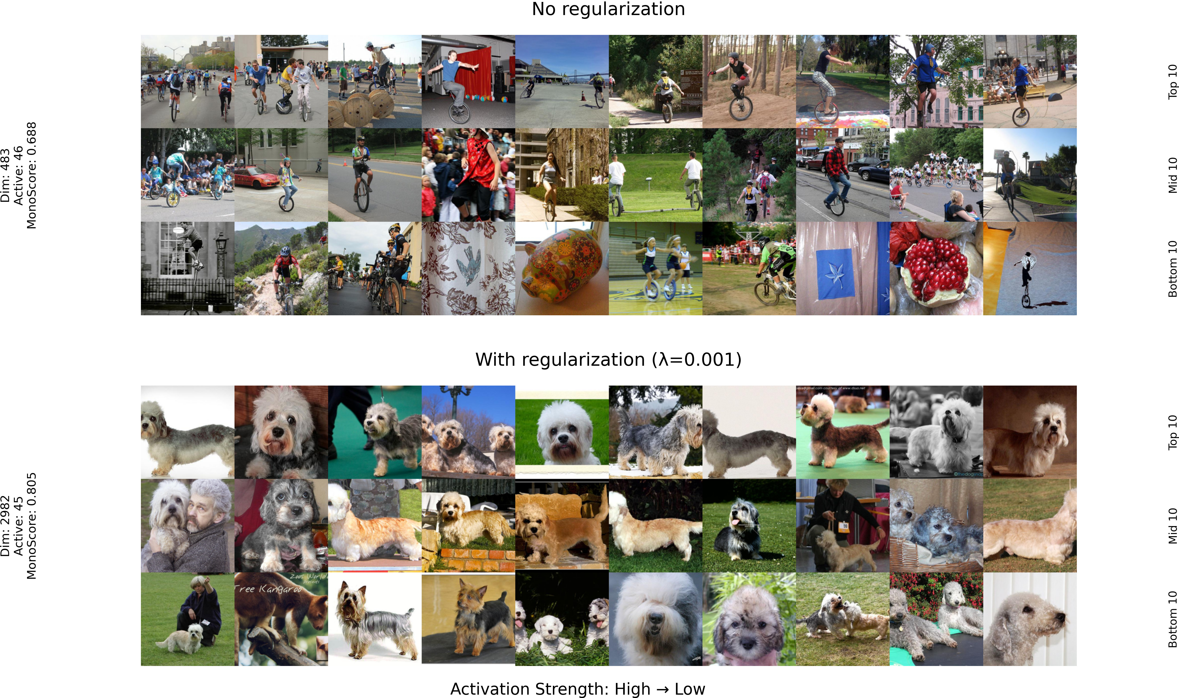
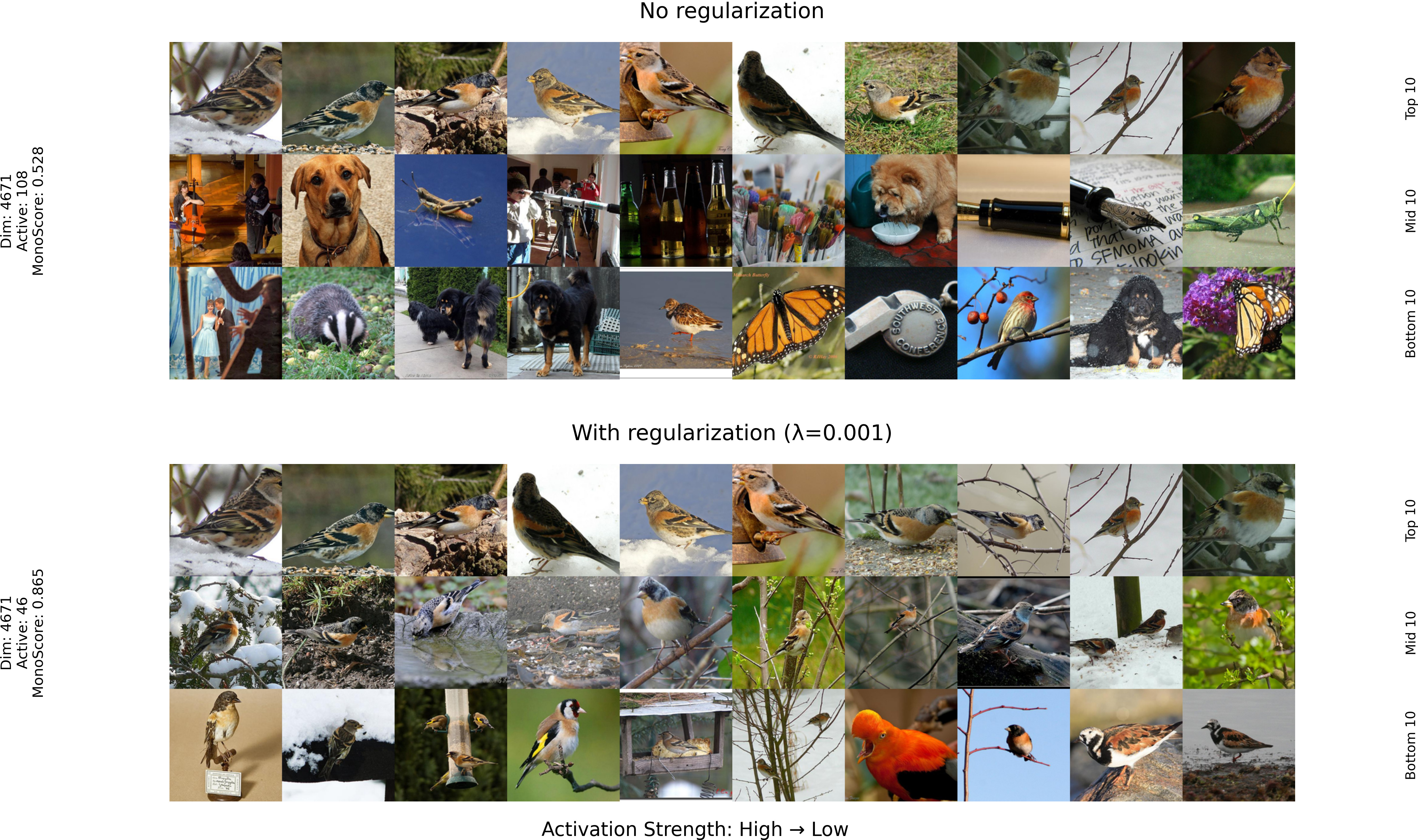
The Monosemanticity Score is intended to quantify how visually and semantically coherent the images activating a latent are. We complement it with a direct qualitative inspection of these images. We focus on the ViT encoder with \(k=32\) and rank the latents by their test-set monosemanticity score, separately for the baseline and for Regularizer 1 (off-support \(\ell_1\)). For a given latent, we examine its top-10, middle-10, and bottom-10 activating images–that is, the images eliciting its strongest, median, and weakest activations—which probes coherence across the full activation range rather than at the peak alone.
We conduct two complementary comparisons. The first is rank-matched: we compare the latent at a given monosemanticity rank with the regularizer against the latent at the same rank without it (in general two distinct units), isolating how coherent a latent of comparable standing is in each model. The second is unit-matched: we compare the same latent (identical position in the dictionary) with and without the regularizer, isolating the effect of the penalty on a fixed unit.
The rank-matched comparison (Figure 2) shows that, with the regularizer, the dominant concept of a latent remains consistent down to its weakest (bottom-10) activations, whereas for the baseline coherence degrades away from the top activations. The unit-matched comparison (Figure 3) shows that a given latent continues to encode the same concept with and without the regularizer, but its set of activating images becomes markedly more coherent.
4.0.0.5 Sparsity effects of the regularizers.
While the regularizers were shown above to improve monosemanticity, their original motivation is to impose an additional sparsity constraint. To visualize their effect on the activation distribution, we sort each test sample’s \(m\) activations in decreasing order and average them rank-by-rank across the ImageNet-1K test set, obtaining the mean magnitude of the \(r\)-th largest activation as a function of rank \(r\). Figure 4 plots this averaged, rank-ordered profile for CLIP ViT-L/14 at \(k=64\), for the baseline and for each regularizer; the red line at rank \(k=64\) separates the activations kept by the Top-\(k\) operator (left) from those it zeroes out (right).
The two regularizers act on this profile in qualitatively different ways. Regularizer 1 (off-support \(\ell_1\)) leaves the kept activations almost unchanged relative to the baseline and only suppresses the off-support tail, consistent with its design. Regularizer 2 (\(\ell_1/\ell_2\) ratio) instead reshapes the entire profile, concentrating mass onto the very top ranks: its largest activation is substantially higher than the baseline’s while the remaining ranks decay much faster. The \(\ell_1/\ell_2\) ratio thus has the more pronounced effect on the activation distribution, whereas the off-support penalty acts only where activations are already small.
So far, our interpretability analysis considered both regularizers and showed that Regularizer 1 yields the larger monosemanticity gains. The activation profiles, however, reveal that Regularizer 2 reshapes the latent geometry far more aggressively. The remaining experiments focus on Regularizer 2, showing that its concentrated geometry brings substantial benefits beyond monosemanticity.
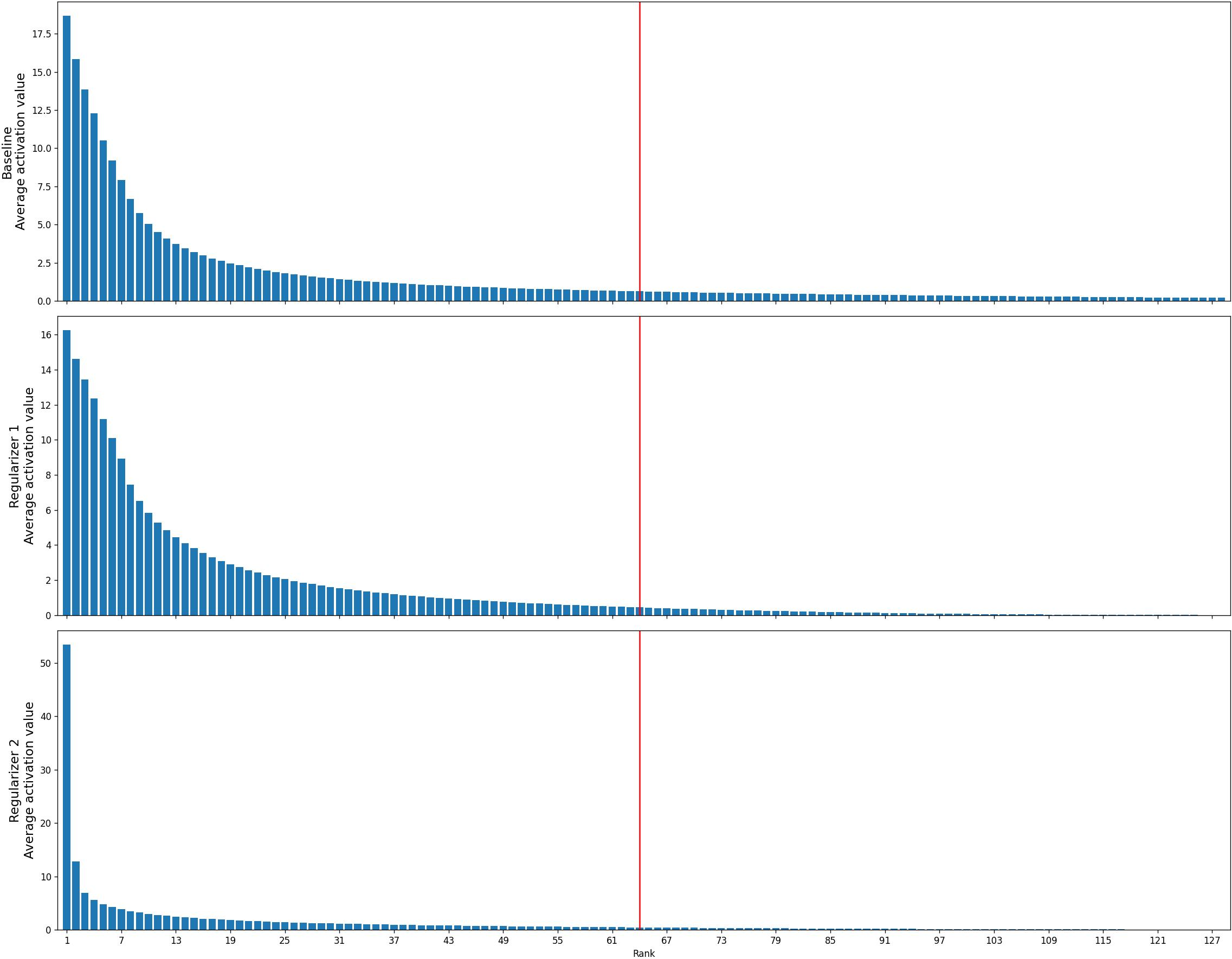

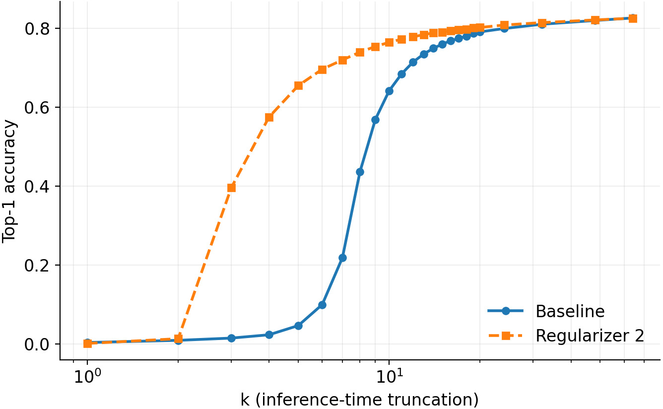
Figure 5: Two consequences of the concentration induced by Regularizer 2 (\(\ell_1/\ell_2\) ratio), on ImageNet-1K with CLIP ViT-L/14. (left) Robustness to the inference-time number of retained units: each panel is a model trained at a fixed \(k\) (left to right: \(k=32, 64, 128\); dotted line) and evaluated while varying \(k_{\text{inf}}\) at inference; both axes are logarithmic. (right) Probing under activation truncation at \(k=64\): a linear probe is trained on codes truncated to their \(k'\) largest activations, and top-1 test accuracy is plotted against \(k'\) (log scale)..
4.0.0.6 Robustness to the inference-time \(k\).
A direct consequence of the concentration induced by Regularizer 2 is that activation magnitudes decay quickly with rank (Figure 4), so that most of the reconstructed signal is carried by a small number of units. This suggests that the exact number of units retained at inference should matter less than for the baseline: keeping slightly fewer or more than the training \(k\) should leave reconstruction largely unchanged. Such a property would mitigate a known limitation of Top-\(k\) SAEs, namely their sensitivity to the arbitrary choice of \(k\) and the resulting overfitting to the training value [7]. To test this, we train Top-\(k\) SAEs on ImageNet-1K with CLIP ViT-L/14 at \(k \in \{32, 64, 128\}\), with and without Regularizer 2, and evaluate each model while varying the number of retained units \(k_{\text{inf}}\) at inference around the training value. We report the normalized reconstruction error (NMSE) as a function of \(k_{\text{inf}}\).
Figure 5 reveals two complementary effects, both more pronounced at larger training \(k\). For \(k_{\text{inf}}\) below the training value (i.e.under truncation), Regularizer 2 attains a consistently lower NMSE than the baseline, and the gap widens as the model is truncated more aggressively–most strikingly at training \(k=128\), where the regularized model degrades far more gracefully. For \(k_{\text{inf}}\) above the training value, the baseline NMSE rises back up, indicating that it has overfit to using exactly \(k\) units, whereas Regularizer 2 remains essentially flat. Together, these show that the concentrated geometry makes reconstruction substantially more robust to the inference-time \(k\).
4.0.0.7 Probing under activation truncation.
If Regularizer 2 concentrates activation magnitude onto fewer units, it should also concentrate the information carried by the code, in the sense that fewer units suffice to identify the class of a sample. We test this by probing the code under activation truncation. For each trained SAE, we form a truncated code by keeping only the \(k'\) largest activations of each sample and zeroing the rest, fit a linear probe on these truncated codes for ImageNet-1K classification (\(1000\) classes), training the probe on the training split and reporting top-1 accuracy on the test split. Sweeping the truncation level \(k'\) yields an accuracy-versus-\(k'\) curve; a curve that rises steeply at small \(k'\) indicates that the discriminative information is packed into few coordinates. We train Top-\(k\) SAEs on ImageNet-1K with CLIP ViT-L/14, SigLIP2, and a supervised ViT-L/16, and compare the baseline against Regularizer 2.
Figure 5 shows the curve for CLIP ViT-L/14 at \(k=64\). The two models reach the same asymptotic test accuracy (\({\approx}0.82\)) once enough units are retained, so the regularizer does not change the total information recoverable from the code; it reaches high accuracy with far fewer units, dominating the baseline across the entire small-budget regime.
To quantify this concentration of discriminative information, we report the normalized area under the accuracy-versus-\(k'\) curve, defined as the AUC over \(k' \in [1, K]\) divided by \(K\); this rescaling places it in \([0,1]\) and keeps it comparable across integration ranges. A higher value indicates that accuracy is attained at smaller truncation levels. We set \(K = 32\), integrating only up to this point because the accuracy curves of the two models converge once enough units are retained, so beyond it their difference adds no discriminative signal and would only attenuate the metric.
Table 3 reports the normalized AUC across all nine configurations, together with the top-1 accuracy at the full budget \(k'=32\). The AUC is higher for Regularizer 2 in every configuration, confirming that it consistently front-loads discriminative information into the leading activations. At the same time, the accuracy at \(k'=32\) is essentially unchanged relative to the baseline, showing that this gain in early-budget accuracy comes at no cost to overall performance.
| Norm.AUC | Top-1 @ \(k'{=}32\) | ||||
|---|---|---|---|---|---|
| 3-4 (lr)5-6 Enc. | \(k\) | Base | Reg. 2 | Base | Reg. 2 |
| CLIP | 32 | 0.683 | 0.731 | 0.815 | 0.815 |
| 64 | 0.607 | 0.726 | 0.810 | 0.814 | |
| 128 | 0.479 | 0.692 | 0.773 | 0.804 | |
| SigLIP | 32 | 0.706 | 0.778 | 0.856 | 0.856 |
| 64 | 0.625 | 0.771 | 0.853 | 0.856 | |
| 128 | 0.485 | 0.757 | 0.803 | 0.851 | |
| ViT | 32 | 0.758 | 0.784 | 0.801 | 0.804 |
| 64 | 0.743 | 0.782 | 0.802 | 0.802 | |
| 128 | 0.752 | 0.755 | 0.801 | 0.802 | |
3pt
4.0.0.8 Necessity of the active-unit mask.
Both regularizers are restricted to the batch-active units–those selected in the Top-\(k\) of at least one sample of the batch (Section 2.2). We motivated this design by noting that an unselected unit receives no gradient from the reconstruction term; penalizing it directly therefore applies a one-sided force that drives its activations to zero and eventually kills the unit. To test this, we repeat every configuration of Tables 1 and 2 with the regularization applied to all units (no mask) and report the resulting number of dead neurons.
Table 4 confirms the claim. Removing the mask increases the number of dead neurons in nearly every configuration, frequently by one to two orders of magnitude (e.g.from \(12\) to \(2426\) dead units for the supervised ViT-L/16 on Open Images V7 at \(k=32\) under Regularizer 1). The few exceptions are configurations in which no units die even without the mask, such as the supervised ViT-L/16 on ImageNet-1K at \(k \in \{64,128\}\). Beyond the increase in dead neurons, the unmasked variant also systematically lowers mean monosemanticity relative to the masked one. The mask is thus necessary both for stability and for the interpretability gains reported above.
| ImageNet-1K | Open Images V7 | |||||
|---|---|---|---|---|---|---|
| 4-5 (lr)6-7 Enc. | \(k\) | Method | Masked | No mask | Masked | No mask |
| CLIP | 32 | Reg. 1 | 26 | 1052 | 40 | 2514 |
| Reg. 2 | 59 | 303 | 45 | 801 | ||
| 64 | Reg. 1 | 1 | 316 | 2 | 837 | |
| Reg. 2 | 10 | 276 | 11 | 319 | ||
| 128 | Reg. 1 | 0 | 27 | 0 | 423 | |
| Reg. 2 | 1 | 69 | 5 | 150 | ||
| SigLIP | 32 | Reg. 1 | 232 | 1066 | 182 | 1438 |
| Reg. 2 | 248 | 428 | 224 | 1107 | ||
| 64 | Reg. 1 | 176 | 595 | 77 | 1205 | |
| Reg. 2 | 255 | 394 | 257 | 858 | ||
| 128 | Reg. 1 | 72 | 301 | 7 | 600 | |
| Reg. 2 | 157 | 257 | 84 | 191 | ||
| ViT | 32 | Reg. 1 | 0 | 625 | 12 | 2426 |
| Reg. 2 | 0 | 490 | 9 | 2052 | ||
| 64 | Reg. 1 | 0 | 0 | 0 | 391 | |
| Reg. 2 | 0 | 0 | 0 | 617 | ||
| 128 | Reg. 1 | 0 | 0 | 0 | 12 | |
| Reg. 2 | 0 | 0 | 0 | 12 | ||
3pt
5 5 Conclusion↩︎
We introduced two sparsity regularizers compatible with the Top-\(k\) architecture, both acting on the activations before the Top-\(k\) selection: an \(\ell_1\) penalty on the off-support units and an \(\ell_1/\ell_2\)-ratio penalty on the full activation vector. Across two datasets, three vision foundation models, and a range of \(k\), both regularizers consistently improve interpretability—measured by monosemanticity and class purity–at no cost to reconstruction quality. Beyond interpretability, we showed that the concentration induced by the \(\ell_1/\ell_2\)-ratio penalty makes reconstruction substantially more robust to the inference-time choice of \(k\) and front-loads discriminative information into the leading units, improving small-budget linear probing.
These results carry a simple message: although the Top-\(k\) SAE was introduced specifically to avoid the \(\ell_1\) penalty and its known drawbacks, it still benefits from an explicit sparsity constraint–provided the constraint acts on the pre-selection activations rather than the sparse code, and is restricted to the batch-active units so as not to create dead latents. Hard architectural sparsity and soft regularization are thus complementary rather than mutually exclusive.
Several directions follow naturally. The regularizers could be extended to other members of the Top-\(k\) family, such as BatchTopK [10] and Matryoshka SAEs [22], whose selection mechanisms differ from the per-sample Top-\(k\) studied here. More broadly, the \(\ell_1/\ell_2\) ratio is a scale-invariant sparsity measure that remains underused in representation learning, and our results suggest it is a promising and largely unexplored tool for shaping the geometry of sparse codes.