Exact and Deterministic Patch Descriptor Retrieval
via Hierarchical Normalization
June 25, 2026
Abstract
We present a patch descriptor retrieval method that returns the exact nearest neighbour—provably identical to exhaustive full-vector search—while evaluating only a small fraction of the database, and does so deterministically: the same (database, query) pair always produces the same result, independent of run order, thread count, or hardware; the output depends on database ordering only in the negligible event of exact inner-product ties (see Theorem [thm:det]). This sets our method apart from approximate nearest-neighbour (ANN) approaches such as HNSW and IVF-PQ, and from Matryoshka-style pipelines built on such indexes, which trade exactness for speed and may return different results across runs. The enabling mechanism is Hierarchical Normalization (HN): a normalisation scheme that replaces the standard L2 normalisation layer and splits the pre-normalisation feature vector into a \(K\)-dim major component with norm \(\sqrt{1{-}\alpha}\) and a \((128{-}K)\)-dim minor component with norm \(\sqrt{\alpha}\). Because the minor inner product is bounded by \(\alpha\) (Cauchy–Schwarz on the prescribed norms), the major similarity plus \(\alpha\) serves as an admissible upper bound on the full similarity: the search scans the \(K\)-dim major component for all entries, then performs full \(128\)-dim evaluation only for the small fraction that cannot be pruned—a branch-and-bound scan that is provably exact. We train HN-modified HardNet on the notredame split of the UBC patch dataset and evaluate on trevi and halfdome. With a cache-optimised Structure-of-Arrays (SoA) layout and \(K{=}8\), \(\alpha{=}1/32\), the search achieves \(\mathbf{13.7\times}\) (trevi) / \(\mathbf{12.7\times}\) (halfdome) wall-clock speed-up over brute-force 128-dim search, with only \(0.4\%\) of entries requiring full 128-dim evaluation. At \(K{=}16\), \(\alpha{=}1/8\)—the recommended operating point—FPR@95 rises only from \(0.0062\) (pretrained baseline) to \(0.0064\) on trevi at \(7.2\times\) speed-up, with \(98.8\%\) of entries bypassing full evaluation.
1 Introduction↩︎
Dense nearest-neighbour search over high-dimensional embedding vectors has become central to modern AI: retrieval-augmented generation (RAG) pipelines for large language models retrieve relevant context by dot-product similarity over billions of text and image embeddings; image authentication systems (e.g.FaceNet-style face verification) compare identity embeddings by L2 distance; and visual place recognition localises a scene by matching query embeddings against a geotagged database. In all these settings, returning an exact and reproducible answer is increasingly important alongside raw speed. Although we evaluate on local patch descriptors, the HN normalisation is agnostic to the embedding type and is directly applicable wherever embeddings are compared by inner product.
Large-scale patch matching requires searching millions of descriptors. With \(D\)-dimensional vectors (128 for HardNet) this costs \(O(DN)\) per query, so production systems often turn to approximate nearest-neighbour (ANN) indexes such as HNSW [2] and IVF-PQ [3]. ANN buys sub-linear—or at minimum cache-efficient—search at two costs that are easy to overlook: (i) it is approximate—the returned item may not be the true nearest neighbour, and (ii) it is non-deterministic—results depend on graph construction order, entry-point selection, thread count, and hardware platform. For A/B testing, result caching, regression tracking, and safety auditing, returning a different or wrong top result across runs is a real liability.
Our key insight is that a descriptor can be trained so that exact search is cheap. By constraining the normalisation, we concentrate \(1{-}\alpha\) of each descriptor’s energy into a compact \(K\)-dim major prefix and cap the remaining minor contribution at \(\alpha\). This gives an admissible upper bound: \(\mathrm{sim}_{\mathrm{full}} \le \mathrm{dot}_K + \alpha\). A branch-and-bound scan over the major prefix then returns the exact nearest neighbour while fully evaluating only the small fraction of entries that could plausibly beat the running best.
Relation to prior work on non-uniform prefix embeddings. The idea of concentrating discriminative information into a compact prefix of an embedding vector—so that the prefix alone can serve as a coarse index—was first disclosed in a patent filed in June 2020 [1], predating subsequent work on elastic or multi-granularity embeddings. Matryoshka Representation Learning (MRL) [4] independently popularised a related training objective for general-purpose representations (NeurIPS 2022). The present paper reproduces and extends the retrieval algorithm described in [1], now with formal proofs of exactness and determinism, and evaluated on the public UBC patch benchmark.
Contributions.
Exact retrieval (Theorem 1). We prove that HN-based two-phase search returns precisely the nearest neighbour of exhaustive full-vector search; the speed-up incurs zero retrieval error.
Determinism (Theorem 2). HN search is reproducible across runs, index builds, and thread counts; given a fixed database ordering it is fully deterministic, and in practice ordering-independent (exact inner-product ties are negligible with floating-point descriptors)—in contrast to HNSW/IVF-PQ and MRL pipelines that rely on them.
Efficiency. A cache-optimised SoA layout with \(K{=}8\), \(\alpha{=}1/32\) achieves \(13.7\times\) (trevi) / \(12.7\times\) (halfdome) wall-clock speed-up on CPU with \(500{,}000\) database entries, with only \(0.4\%\) of entries requiring full 128-dim evaluation (see Table 3 for the full quality–speed Pareto frontier). At \(K{=}16\), \(\alpha{=}1/8\) the FPR@95 cost is only \(0.0002\) on trevi at \(7.2\times\) speed-up.
2 Related Work↩︎
2.0.0.1 Local feature descriptors.
Hand-crafted descriptors (SIFT [5], ORB [6]) have largely been supplanted by learned descriptors [7]. HardNet [7] trains a 128-dim descriptor with hard-negative triplet loss, setting the state of the art on the UBC patch benchmark.
2.0.0.2 Approximate nearest-neighbour search.
FAISS [8], HNSW [2], and IVF-PQ [3] accelerate retrieval via quantisation and graph indexes. ScaNN [9] improves inner-product quantisation via anisotropic scoring; DiskANN [10] scales graph indexes to disk for billion-scale retrieval. Binary hashing methods (LSH [11]) achieve sub-linear search via compact codes at the cost of recall guarantees. All of these methods are approximate or non-deterministic by construction. Our method is orthogonal to these approaches; building a sub-linear index on the \(K\)-dim major for Phase-1 is theoretically possible, though whether it helps with HN-trained descriptors in practice remains an open question (see Section 7).
2.0.0.3 Non-uniform prefix embeddings.
The concept of assigning non-uniform importance to dimensions and using a compact prefix for coarse-to-fine retrieval was first disclosed in a patent filed June 24, 2020 [1]. Matryoshka Representation Learning [4] independently introduced a training scheme that makes representations elastic in size (NeurIPS 2022), enabling nested sub-vectors to be used as approximate indexes at varying granularities. Unlike HN, MRL makes no admissibility guarantee: MRL retrieval pipelines rely on ANN indexes for efficiency and therefore inherit their approximate, non-deterministic behaviour.
2.0.0.4 Cascaded/hierarchical retrieval.
Cascaded hashing [12] and multi-resolution methods reduce computation by progressively refining candidate sets. HN achieves a similar effect with a single normalisation and a mathematically grounded, provably exact pruning criterion.
3 Hierarchical Normalization↩︎
3.1 Formulation↩︎
HN replaces the standard L2 normalisation layer of the descriptor network. Let \(\mathbf{f} \in \mathbb{R}^D\) be the pre-normalisation feature vector. We split \(\mathbf{f}\) into a major prefix of \(K\) dimensions and a minor suffix of \(D - K\) dimensions, normalising each part to prescribed norms:
\[\mathbf{f}_{\mathrm{major}} = \sqrt{1-\alpha}\,\frac{\mathbf{f}_{[:K]}}{\|\mathbf{f}_{[:K]}\|}, \qquad \mathbf{f}_{\mathrm{minor}} = \sqrt{\alpha}\,\frac{\mathbf{f}_{[K:]}}{\|\mathbf{f}_{[K:]}\|}, \label{eq:hn}\tag{1}\]
so that \(\|\mathbf{f}_{\mathrm{major}}\|^2 = 1{-}\alpha\), \(\|\mathbf{f}_{\mathrm{minor}}\|^2 = \alpha\), and the full vector \([\mathbf{f}_{\mathrm{major}},\mathbf{f}_{\mathrm{minor}}]\) has unit norm. The scalar \(\alpha \in [0,1)\) controls the energy split.
Why fine-tuning is necessary. HardNet is trained to maximise discriminability via hard-negative triplet loss; as a result, energy tends to spread uniformly across all 128 dimensions. Replacing the L2 normalisation with HN post-hoc—without any further training—does not concentrate energy in the major subspace. The major component then represents only an arbitrary \(K\)-dimensional slice of a uniformly distributed descriptor, so Phase-1 scores are weaker predictors of the full inner product and fewer database entries are pruned. Concretely, at \(K{=}16\), \(\alpha{=}1/8\) on \(N{=}99{,}000\) UBC patches, applying HN post-hoc to pretrained HardNet gives Phase-2% \(= 9.2\%\) on trevi; fine-tuning reduces this to \(1.1\%\)—an \(8{\times}\) improvement that directly translates to higher wall-clock speed-up. Fine-tuning shifts energy toward the major component, making the first \(K\) dimensions carry the bulk of the discriminative signal and Phase-1 scores reliable predictors of the full ranking.
3.2 Admissible Bound↩︎
For query \(\mathbf{q}\) and database entry \(\mathbf{x}\) (both HN-normalised network outputs), the inner product decomposes naturally as
\[\langle \mathbf{q}, \mathbf{x} \rangle = \underbrace{\langle \mathbf{q}_{\mathrm{major}}, \mathbf{x}_{\mathrm{major}}\rangle}_{\mathrm{dot}_{K}(\mathbf{q},\mathbf{x})} + \underbrace{\langle \mathbf{q}_{\mathrm{minor}}, \mathbf{x}_{\mathrm{minor}}\rangle}_{\le\,\alpha}. \label{eq:decomp}\tag{2}\]
By Cauchy–Schwarz, \(\langle\mathbf{q}_{\mathrm{minor}},\mathbf{x}_{\mathrm{minor}}\rangle \le \|\mathbf{q}_{\mathrm{minor}}\|\|\mathbf{x}_{\mathrm{minor}}\| = \alpha\), so we obtain the admissible upper bound:
\[\boxed{ \langle \mathbf{q}, \mathbf{x} \rangle \;\le\; \mathrm{dot}_{K}(\mathbf{q}, \mathbf{x}) + \alpha. } \label{eq:bound}\tag{3}\]
The bound is tight when the minor components are identical; it is independent of database size and holds for any \(\alpha \in [0,1)\).
3.3 Exact and Deterministic Two-Phase Search↩︎
Figure 1: 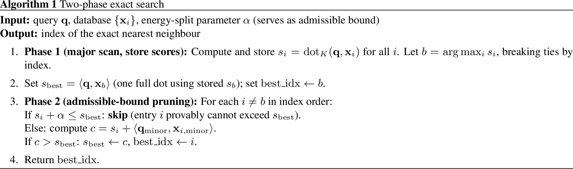 .
.
Theorem 1 (Exactness). For any database and query using descriptors satisfying Eq. 1 , Algorithm 1 returns the same index as exhaustive full-vector search.
Proof. For any entry \(i\) skipped in Phase 2: the skip condition gives \(s_i + \alpha \le s_{\mathrm{best}}\). By Eq. 3 , \(\langle\mathbf{q},\mathbf{x}_i\rangle \le s_i + \alpha \le s_{\mathrm{best}}\), so entry \(i\) provably cannot exceed the current best. Entry \(b\) is fully evaluated first, and \(s_{\mathrm{best}}\) is updated for every non-skipped entry; hence it equals the maximum inner product over all fully evaluated entries. Since every skipped entry is known to lie at or below \(s_{\mathrm{best}}\) without computing its full inner product, \(s_{\mathrm{best}}\) attains the global maximum; the returned index is therefore the global nearest neighbour. ◻
Theorem 2 (Determinism). For a fixed database ordering and tie-breaking rule, Algorithm 1 produces a unique output for each query, reproducible across runs on the same platform.
Proof. \(\mathrm{dot}_K(\mathbf{q},\mathbf{x}_i)\) is a deterministic matrix–vector product; ties are resolved by index, giving a total order. The Phase-2 traversal, bound test, and maximisation use no randomness. The output is a deterministic function of (database, query, database ordering). ◻
Remark (ordering dependence in practice). The dependence on database ordering in Theorem 2 arises only when two entries share an identical full inner product with the query—an exact numerical tie resolved by index. With 32-bit floating-point HN-normalised descriptors optimised by gradient descent, such ties occur with negligible probability, so the output is effectively independent of database ordering for virtually all (database, query) pairs. In contrast, with quantised descriptors (e.g.-bit integer or binary codes), the discrete value space makes exact ties considerably more likely; in those settings, database ordering becomes a meaningful part of the determinism guarantee and should be explicitly fixed and documented.
Note on Phase-2 scan order. Algorithm 1 traverses entries in index order rather than sorted by descending \(s_i\). A sorted scan would enable early loop termination (once \(s_i + \alpha < s_{\mathrm{best}}\), all remaining entries are prunable), but sorting adds \(O(N\log N)\) overhead. In the SoA layout the score buffer (2 MB for \(K{=}16\), \(N{=}500{,}000\)) fits entirely in the \(12\) MB L3 cache, so the \(N\) sequential score reads in Phase-2 are cheap; the index-order design avoids sorting while incurring negligible memory bandwidth cost.
Together, Theorems 1 and 2 separate HN from ANN methods (HNSW, IVF-PQ) and from MRL pipelines built on such indexes: those trade exactness for speed and produce run-varying results, whereas HN reproduces the exhaustive-search result every time.
4 Experimental Setup↩︎
4.0.0.1 Backbone.
HardNet [7] with publicly available pre-trained weights, modified by replacing the final L2 normalisation with \(\mathrm{HN}_\alpha\).
4.0.0.2 Training.
All models are initialised from the pretrained HardNet weights and fine-tuned on the notredame split of the UBC patch dataset [13] with TripletMarginLoss (margin \(1.0\)), Adam (\(\mathrm{lr}{=}10^{-4}\)), batch size 32 (empirically chosen for the fine-tuning regime; larger batches yielded no improvement). We report two settings: \(K{=}16\) (30 epochs) and \(K{=}8\) (10 epochs); epoch counts were determined by monitoring the training loss on a held-out validation subset and stopping when the loss plateaued. Because HN fine-tuning only needs to shift energy into the major subspace—not relearn full discriminability—and because HardNet’s original training data is no longer readily accessible (retraining on substitute data degrades quality), a short fine-tuning schedule suffices for both settings.
4.0.0.3 Dataset.
The UBC patch dataset [13] provides three independent patch collections: notredame (train), trevi and halfdome (test). Pre-extracted patches are used directly, without a keypoint detector front-end. Cross-scene evaluation measures generalisation under domain shift.
4.0.0.4 Metric.
FPR@95: false positive rate at \(95\%\) true positive rate. Lower is better.
5 Experiments↩︎
5.1 Descriptor Quality↩︎
| Method | \(\alpha\) | trevi | halfdome |
|---|---|---|---|
| SIFT | — | 0.0617 | 0.1415 |
| (pretrained)\(^\dagger\) | — | 0.0062 | 0.0201 |
| \(K{=}16\), \(\alpha{=}0\) | 0 | 0.0109 | 0.0787 |
| \(K{=}16\), \(\alpha{=}1/32\) | 1/32 | 0.0089 | 0.0653 |
| \(K{=}16\), \(\alpha{=}1/16\) | 1/16 | 0.0078 | 0.0539 |
| \(K{=}16\), \(\alpha{=}1/8\) | 1/8 | 0.0064 | 0.0462 |
| \(K{=}16\), \(\alpha{=}1/4\) | 1/4 | 0.0056 | 0.0414 |
| \(K{=}8\), \(\alpha{=}0\) | 0 | 0.0447 | 0.2243 |
| \(K{=}8\), \(\alpha{=}1/32\) | 1/32 | 0.0397 | 0.1837 |
| \(K{=}8\), \(\alpha{=}1/16\) | 1/16 | 0.0339 | 0.1565 |
| \(K{=}8\), \(\alpha{=}1/8\) | 1/8 | 0.0270 | 0.1186 |
| \(K{=}8\), \(\alpha{=}1/4\) | 1/4 | 0.0164 | 0.0904 |
4pt
5.1.0.1 \(K{=}16\).
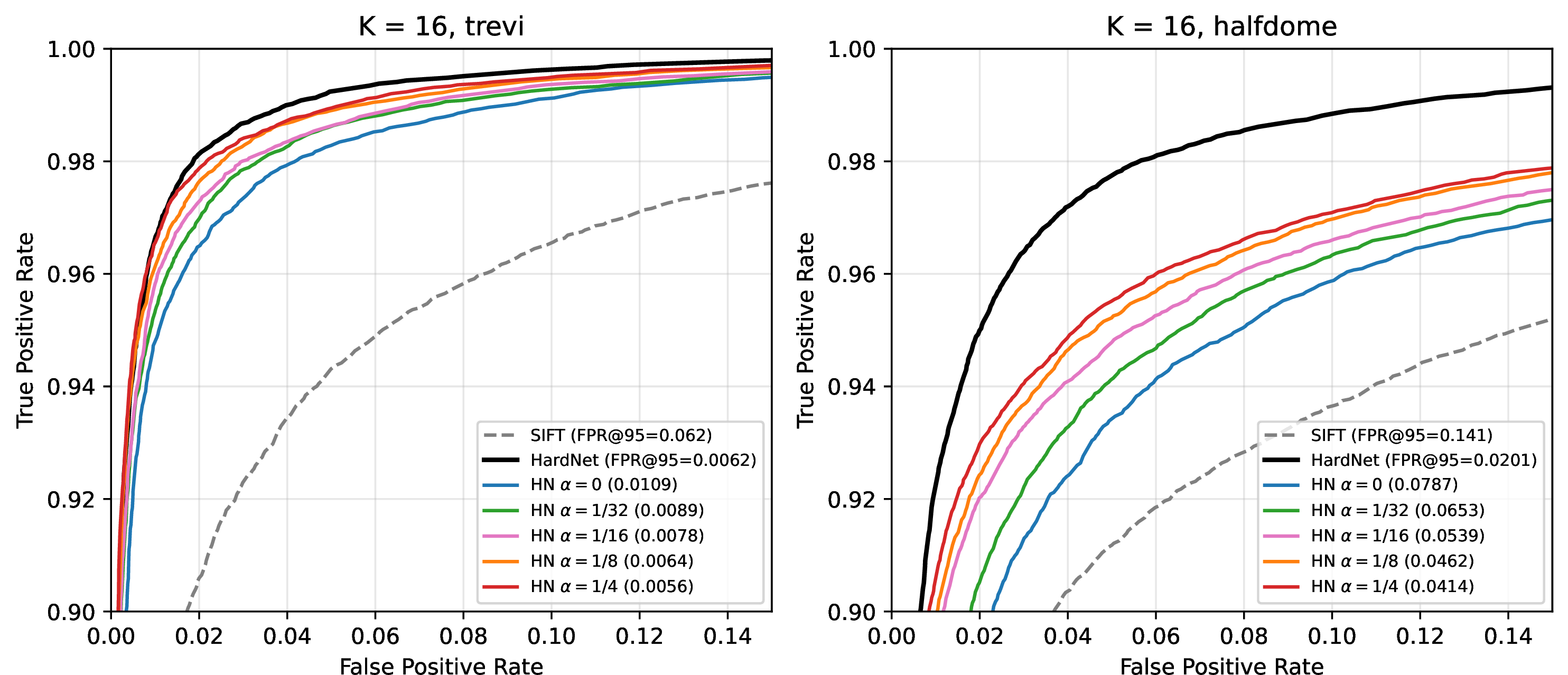
Quality improves monotonically with \(\alpha\). At \(\alpha{=}0\) (pure major-only), FPR@95 is \(0.0109\) on trevi. At \(\alpha{=}1/8\) the gap to the pretrained baseline is already negligible (\(0.0002\)), confirming that HN normalisation preserves almost all discriminative information at a substantial speed-up. At \(\alpha{=}1/4\), FPR@95 reaches \(0.0056\)—below the pretrained baseline of \(0.0062\)—because HN fine-tuning reshapes the descriptor geometry to concentrate energy in the major subspace; this restructuring incidentally improves cross-scene discriminability, consistent with known regularisation effects of fine-tuning under constrained normalisation. All configurations satisfy the exactness guarantee of Theorem 1. Figure 2 shows the full ROC curves.
5.1.0.2 \(K{=}8\).
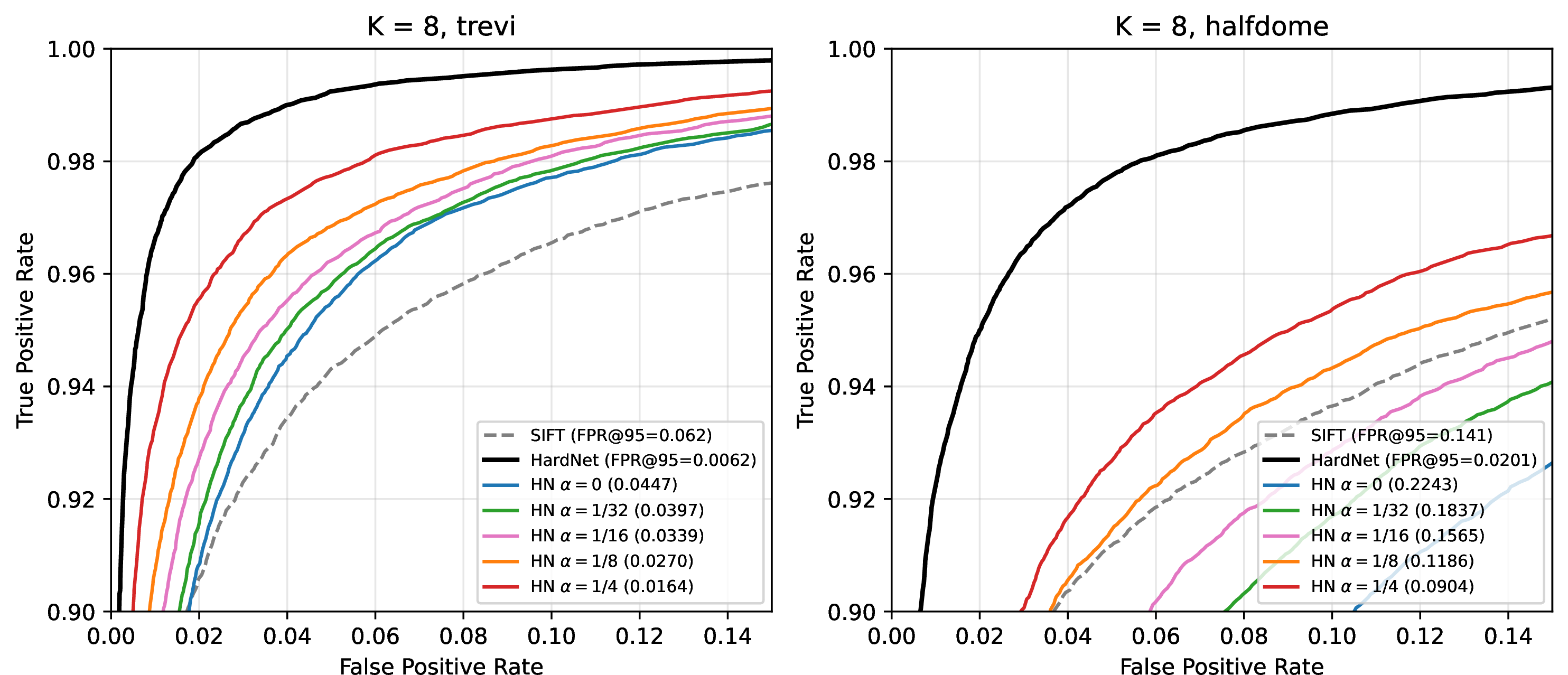
Quality improves monotonically with \(\alpha\), mirroring the \(K{=}16\) trend. At \(\alpha{=}1/4\), FPR@95 reaches \(0.0164\) on trevi and \(0.0904\) on halfdome; \(\alpha{=}1/8\) gives \(0.0270\) on trevi, already well below SIFT (\(0.0617\)). The larger gap vs.the pretrained baseline reflects the greater challenge of representing information with only an 8-dim major prefix. Figure 3 shows the full ROC curves.
5.1.0.3 Effect of \(\alpha\).
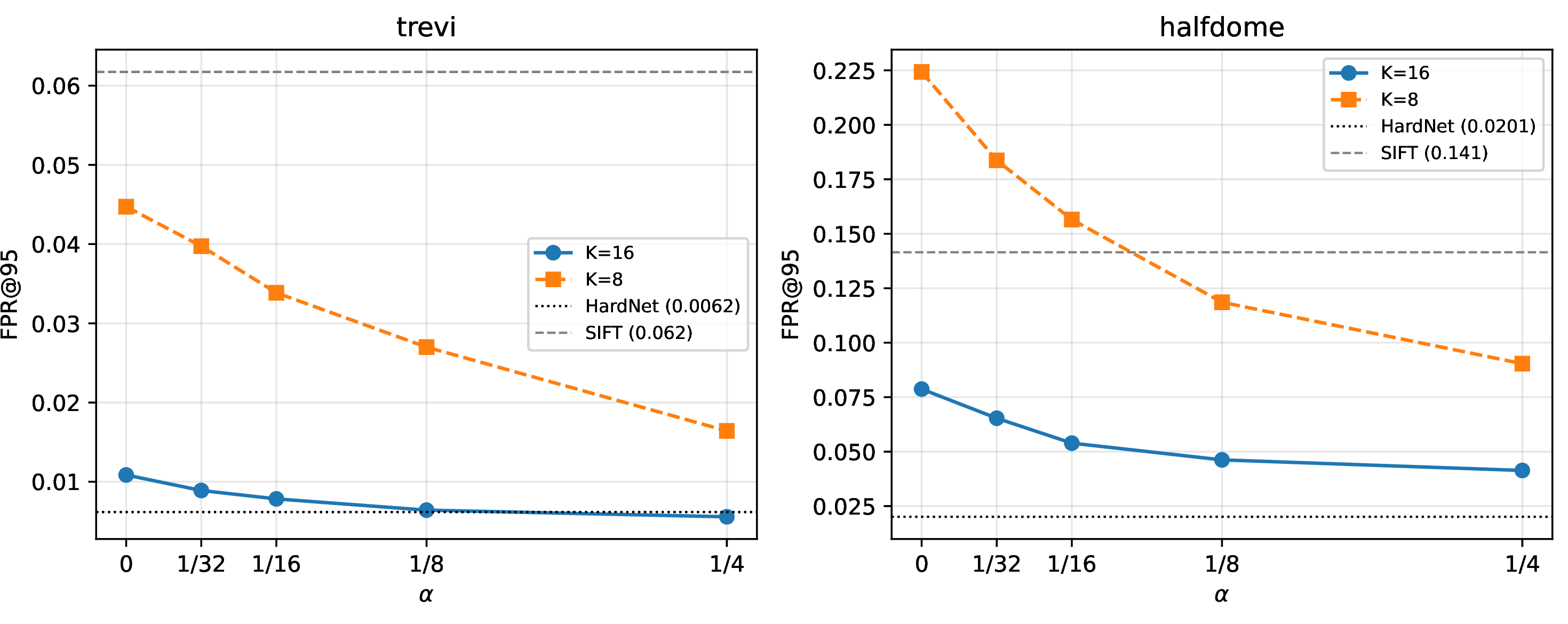
Across both \(K\) settings, larger \(\alpha\) consistently reduces FPR: with greater \(\alpha\), more energy is allocated to the \((128{-}K)\)-dim minor component, spreading discriminative information across additional dimensions and enabling a richer overall descriptor representation. At \(K{=}16\), the FPR improvement from \(\alpha{=}1/32\) to \(\alpha{=}1/4\) spans only \(0.0033\) on trevi; at \(K{=}8\) the same range spans \(0.0233\), confirming gradual and stable improvement in both settings. Figure 4 shows this trend across both scenes.
5.1.0.4 Note on halfdome vs.trevi.
FPR@95 is consistently higher on halfdome across all configurations. This is not specific to HN: the pretrained HardNet baseline already shows \(0.0201\) on halfdome vs.\(0.0062\) on trevi, reflecting greater photometric and viewpoint variation in the halfdome scene. The relative advantage of HN configurations over SIFT is maintained on both scenes.
5.2 Quality–Speed Trade-off↩︎
| Method | trevi | halfdome | ||
|---|---|---|---|---|
| 2-3(lr)4-5 | FPR@95 | Speed | FPR@95 | Speed |
| pretrained | 0.0062 | \(1.0\times\) | 0.0201 | \(1.0\times\) |
| \(K{=}16\), \(\alpha{=}1/8\) | 0.0064 | \(7.2\times\) | 0.0462 | \(5.8\times\) |
| \(K{=}8\), \(\alpha{=}1/8\) | 0.0270 | \(10.1\times\) | 0.1186 | \(5.4\times\) |
2pt
\(K{=}16\) trades a small quality cost (\(+0.0002\) FPR on trevi) for a \(7.2\times\) speed-up with full exactness. At \(\alpha{=}1/8\), \(K{=}8\) achieves higher throughput on trevi (\(10.1\times\) vs.\(7.2\times\)) at a larger quality cost; on halfdome the elevated Phase-2% (\(6.6\%\) vs.\(2.8\%\)) reverses this advantage (\(5.4\times\) vs.\(5.8\times\)), making \(K{=}8\) most useful when Phase-2% stays low. Figure 5 visualises the full Pareto frontier.
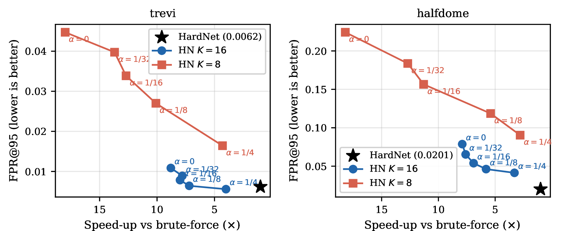
6 Speed Analysis↩︎
6.1 Memory Layout: SoA↩︎
In the conventional Array of Structures (AoS) layout, the \(K\)-dim major scan must load all 128 floats per entry (\(512\) bytes), wasting cache. A Structure of Arrays (SoA) layout stores majors and minors in separate contiguous arrays. For \(K{=}8\) and \(N{=}500{,}000\), the major array is \(16\) MB—versus \(256\) MB for the full descriptor bank—reducing memory bandwidth by \(16\times\). For \(K{=}16\), the major array is \(32\) MB.
6.2 Wall-clock Benchmark↩︎
| \(K\) | \(\alpha\) | trevi | halfdome | ||
|---|---|---|---|---|---|
| 3-4(lr)5-6 | SpeedHier | Phase2% | SpeedHier | Phase2% | |
| 16 | 0 | \(8.8\times\) | 0.0% | \(7.9\times\) | 0.0% |
| 16 | 1/32 | \(7.8\times\) | 0.4% | \(7.6\times\) | 0.5% |
| 16 | 1/16 | \(8.0\times\) | 0.6% | \(6.9\times\) | 1.1% |
| 16 | 1/8 | \(7.2\times\) | 1.2% | \(5.8\times\) | 2.8% |
| 16 | 1/4 | \(4.0\times\) | 5.5% | \(3.3\times\) | 6.5% |
| 8 | 0 | \(18.0\times\) | 0.0% | \(18.2\times\) | 0.0% |
| 8 | 1/32 | \(13.7\times\) | 0.4% | \(12.7\times\) | 0.6% |
| 8 | 1/16 | \(12.7\times\) | 0.6% | \(11.3\times\) | 1.0% |
| 8 | 1/8 | \(10.1\times\) | 1.5% | \(5.4\times\) | 6.6% |
| 8 | 1/4 | \(4.3\times\) | 6.6% | \(2.8\times\) | 11.5% |
3.5pt
At \(K{=}8\), the 16 MB major array is \(16\times\) smaller than the full descriptor bank (256 MB), reducing memory pressure and achieving up to \(18.2\times\) speed-up (\(18.0\times\) on trevi, \(18.2\times\) on halfdome); the 16 MB buffer is close to the \(12\) MB L3 boundary, so partial caching amplifies the bandwidth advantage beyond the nominal \(16\times\) ratio. At \(K{=}16\), peak speed is \(8.8\times\) (trevi, \(\alpha{=}0\)); the larger 32 MB major array exceeds L3 and is fully bandwidth-bound, consistent with the \(8\times\) bandwidth ratio of 32 MB vs. MB. For \(\alpha{\le}1/8\), Phase-2 rates stay below \(2\%\) on trevi and below \(7\%\) on halfdome; at \(\alpha{=}1/4\), Phase-2 rises to at most \(6.6\%\) on trevi and \(11.5\%\) on halfdome (\(K{=}8\)), so the exactness overhead (Theorem 1) is negligible in practice. A notable exception to the decreasing-speed-with-\(\alpha\) trend is \(K{=}8\), \(\alpha{=}0\): at \(\alpha{=}0\), HN normalisation sets all 120 minor components to exactly zero, so Phase 2 never accesses the 240 MB minor array at all. Any \(\alpha{>}0\) forces even a handful of Phase-2 entries (\({\approx}2{,}000\) at \(\alpha{=}1/32\)) to issue random reads into the 240 MB minor array, causing L3 misses and a sharp drop from \(18.0\times\) to \(13.7\times\). Minor fluctuations in Table 3 (e.g.\(K{=}16\) trevi, \(\alpha{=}1/32\) vs.\(1/16\)) are within timing noise; the overall trend is decreasing speedup with increasing \(\alpha\). The largest scene-dependent variation is at \(K{=}8\), \(\alpha{=}1/8\): trevi achieves \(10.1\times\) while halfdome achieves \(5.4\times\). Halfdome’s greater photometric variation makes the 8-dimensional major subspace less discriminative, raising Phase-2% from \(1.5\%\) (trevi) to \(6.6\%\) (halfdome); the resulting \({\sim}33{,}000\) random accesses into the \(240\) MB minor array saturate the \(12\) MB L3 cache. With Phase-1 at \(4\) M FLOPs (\(N{\times}8\)) and Phase-2 at \(4\) M FLOPs (\(33{,}000{\times}120\)), the FLOP model predicts \(64/8 = 8\times\) speed-up. The observed \(5.4\times\) falls below this prediction because the \(33{,}000\) random Phase-2 accesses are latency-bound (L3 cache misses), not throughput-bound—while the lower-Phase-2 trevi case remains bandwidth-dominated at \(10.1\times\).
6.2.0.1 FLOP analysis.
At \(K{=}16\), \(\alpha{=}1/32\) on trevi (Phase2 \(= 0.4\%\)): \[\begin{align} \text{Full 128-dim:} &\quad N{\times}128 = 64\text{M} \\ \text{Phase~1 (major + store):} &\quad N{\times}16 = 8\text{M} \\ \text{Phase~2 (check stored):} &\quad {\approx}\,0\text{M (L3)} \\ \text{Phase~2 (full, 0.4\%):} &\quad 0.004N{\times}(112{+}\tau) \approx 0.2\text{M}{+}2{,}000\tau \\ \text{Total:} &\quad \approx 8.2\text{M}{+}2{,}000\tau \end{align}\] The FLOP ratio predicts \(\approx7.8\times\) speed-up, consistent with the observed \(7.8\times\) in Table 3, where \(\tau\) denotes the DRAM read latency per Phase-2 entry in FLOP-equivalent units; at \(2{,}000\) entries, \(2{,}000\tau\) is small relative to \(8.2\) M. Phase 1 writes the \(N\) major scores (2 MB) to a score buffer that resides in L3 cache; Phase 2 reads this buffer sequentially at negligible cost. The rare Phase-2 full evaluations (\(0.4\%\), \({\approx}2{,}000\) entries) access the 224 MB minor array, which is entirely cold at this point: the SoA layout ensures Phase 1 never touches the minor array, so every Phase-2 access is a first-time DRAM read. At only \(2{,}000\) such accesses, the total latency overhead is negligible.
At \(\alpha{=}0\), HN normalisation sets the minor components to exactly zero, so Phase 2 requires no dot-product computation at all—only the 2 MB score buffer is read for comparison. The bandwidth ratio of the 32 MB major array to the 256 MB full descriptor bank is \(8\times\); the observed \(8.8\times\) (\(K{=}16\), trevi) is consistent with this prediction.
7 Discussion↩︎
7.0.0.1 Why determinism matters.
Modern retrieval systems benefit directly from reproducible results. Caching requires that the same query always returns the same item; A/B testing requires that both branches search the same result space; regression tracking requires that a code change—not hardware or thread scheduling—explains any difference in top-1 output. ANN indexes (HNSW, IVF-PQ) and MRL pipelines built on them fail all three: graph-build order and entry-point selection cause query-time non-determinism. HN satisfies all three by construction (Theorem 2).
7.0.0.2 Why exactness matters.
ANN search introduces silent errors: the returned item may look correct but not be the true nearest neighbour. In safety-critical matching (e.g.forensic image identification, visual place recognition for autonomous navigation), this is unacceptable. HN provides a mathematical certificate of correctness (Theorem 1): the returned result is always the true nearest neighbour.
7.0.0.3 Speed comparison with HNSW.
Reviewers naturally ask how HN speed compares to HNSW, which achieves far higher throughput via approximation. We benchmarked both methods in the same C++ binary on the same machine using \(N{=}99{,}000\) UBC Trevi descriptors (fine-tuned HN, 128-dim, inner-product space; HNSW: \(M{=}16\), efconstruction\(=200\); HNSW was benchmarked on trevi only). On halfdome at \(N{=}99{,}000\), HN \(K{=}16\) achieves \(12.1\)–\(12.9\times\) across \(\alpha{=}0\)–\(1/8\) and \(10.3\times\) at \(\alpha{=}1/4\), consistent with the trevi pattern. Results for trevi are summarised in Table 4.
| Method | Recall@1† | Speed-up | ||
|---|---|---|---|---|
| 3-5 | \(N{=}1\text{K}\) | \(N{=}5\text{K}\) | \(N{=}99\text{K}\) | |
| Brute-force | 100% (exact) | \(1.0\times\) | \(1.0\times\) | \(1.0\times\) |
| \(K{=}16\), \(\alpha{=}0\) (exact) | 100% (proven) | — | — | \(12.7\times\) |
| \(K{=}16\), \(\alpha{=}1/32\) (exact) | 100% (proven) | — | — | \(12.6\times\) |
| \(K{=}16\), \(\alpha{=}1/16\) (exact) | 100% (proven) | — | — | \(12.6\times\) |
| \(K{=}16\), \(\alpha{=}1/8\) (exact) | 100% (proven) | \(\mathbf{9.5\times}\) | \(9.5\times\) | \(12.5\times\) |
| \(K{=}16\), \(\alpha{=}1/4\) (exact) | 100% (proven) | — | — | \(10.4\times\) |
| HNSW ef\(=10\) | 95–98%* | \(7.2\times\) | \(27.6\times\) | \(349\times\) |
| HNSW ef\(=50\) | 99.9%* | \(2.3\times\) | \(7.8\times\) | \(111.9\times\) |
| HNSW ef\(=100\) | 100%* | \(1.4\times\) | \(4.8\times\) | \(63.5\times\) |
| HNSW ef\(=200\) | 100%* | \(0.9\times\) | \(2.9\times\) | \(35.3\times\) |
| HNSW ef\(=500\) | 100%* | \(0.5\times\) | \(1.3\times\) | \(15.8\times\) |
2pt
Four observations follow. (i) HNSW is considerably faster at large \(N\). At ef\(=50\), HNSW achieves \(111.9\times\) vs.HN’s \(12.5\times\) (\(K{=}16\)) at \(N{=}99{,}000\). At the larger \(N{=}500{,}000\) scale (Table 3), \(K{=}16\) drops to \(7.2\times\): the 32 MB major buffer exceeds the 12 MB L3 cache, incurring memory-bandwidth overhead. \(K{=}8\), by contrast, maintains \(18.0\times\) at \(N{=}500{,}000\) because its 16 MB major buffer is close to the L3 boundary and benefits from partial caching. Even at ef\(=500\), HNSW reaches \(15.8\times\). (ii) HNSW’s recall is scale-dependent and unguaranteed. At \(N{=}99{,}000\), ef\(=100\) and above achieve 100% empirical recall on this dataset. On synthetic data at \(N{=}500{,}000\), ef\(=50\) drops to \(\approx\!94\%\) recall, and the ef required for full recall grows with \(N\). The safe ef value cannot be determined without a ground-truth oracle. (iii) HN provides a formal correctness certificate. Theorem 1 proves that HN never returns a wrong result, independent of dataset, size, or hardware ordering. For applications requiring auditable exactness—authentication, forensics, safety-critical navigation—this guarantee is irreplaceable, and no ef setting can provide it through HNSW. (iv) HN’s speed-up is N-independent; HNSW’s grows with \(N\). At \(N{=}5{,}000\), HN achieves \(9.5\times\)—only modestly lower than \(12.5\times\) at \(N{=}99{,}000\)—while HNSW ef\(=50\) drops to \(7.8\times\), falling below HN. At \(N{=}1{,}000\) (typical AR map: 300–1000 3-D landmarks), HN still achieves \(9.5\times\) while every HNSW setting falls below it: ef\(=10\) reaches only \(7.2\times\) with 98% recall, and ef\(\ge 200\) is slower than brute-force. HN’s phase-2 pruning rate is a property of the descriptor distribution alone, while HNSW’s advantage grows as \(N/\log N\) and disappears at small \(N\).
7.0.0.4 Choice of \(\alpha\) and \(K\).
The quality–speed trade-off is monotone: larger \(K\) or larger \(\alpha\) improves quality and reduces speed. The quality–speed curve for \(K{=}16\) has a pronounced elbow near \(\alpha{=}1/8\): for \(\alpha\in\{1/32,1/16,1/8\}\) the HN speed-up stays nearly constant (\(12.5\)–\(12.6\times\) on trevi; Table 4) while FPR@95 falls from \(0.0089\) to \(0.0064\). Increasing to \(\alpha{=}1/4\) reduces the speed-up to \(10.4\times\) on trevi (Table 4; \(10.3\times\) on halfdome) at \(N{=}99{,}000\) and \(4.0\times\)/\(3.3\times\) at \(N{=}500{,}000\) (Table 3), for a smaller quality gain (\(0.0064\to0.0056\)). We therefore recommend \(K{=}16\), \(\alpha{=}1/8\) as the default operating point, at the knee of the \(N{=}99{,}000\) quality–speed curve (Table 4), corresponding to \(7.2\times\) speed-up at \(N{=}500{,}000\) (Table 2). \(K{=}8\), \(\alpha{=}0\) maximises throughput (\(18.0\times\) on trevi / \(18.2\times\) on halfdome, FPR@95 \(= 0.0447\) / \(0.2243\)). Practitioners can select any \((K, \alpha)\) point on the Pareto frontier without sacrificing exactness or determinism.
7.0.0.5 Relation to PCA.
Standard PCA applied post-hoc to HardNet descriptors yields no useful low-dimensional compression. HardNet is trained with hard-negative triplet loss to maximise discriminability, which tends to distribute information uniformly across all 128 dimensions; PCA therefore finds no dominant principal components, and truncating to \(K\) dimensions discards roughly \(1 - K/128\) of the discriminative signal irrespective of which \(K\) are chosen. HN circumvents this by shaping the representation during training. Gradient flow is weighted \((1{-}\alpha)\) toward the major component and \(\alpha\) toward the minor, so the network actively encodes its most discriminative features into the first \(K\) dimensions. This is analogous to active PCA: rather than passively discovering principal components in a fixed embedding, HN trains the embedding so that a known prefix becomes the principal subspace—one whose information concentration is a learned property, not a post-hoc accident.
7.0.0.6 Power-of-two \(\alpha\).
The experimental \(\alpha\) values \(\{1/32, 1/16, 1/8, 1/4\}\) are all powers of two, a natural choice: in quantised implementations, the admissible threshold \(+\alpha = 2^{-n}\) maps to a single integer unit shift, and the relative scale between major and minor components aligns with integer bit widths. We leave a systematic study of fixed-point HN to future work.
7.0.0.7 Soft ANN mode via threshold relaxation.
Algorithm 1 can be extended to a tunable ANN mode by replacing the admissible threshold \(\alpha\) with a smaller value \(\beta < \alpha\) in the skip condition. At \(\beta{=}\alpha\) the algorithm is provably exact (Theorem 1); decreasing \(\beta\) toward zero trades exactness for additional pruning. This single-parameter spectrum—exact at one end, aggressive ANN at the other—requires no structural change to the index. We leave a systematic evaluation of this trade-off to future work.
7.0.0.8 Combination with ANN indexes.
In principle, the \(K\)-dim major vectors could be indexed (e.g.\(k\)-d tree, PQ) to make Phase-1 sub-linear. The lower dimensionality (\(K{=}8\) or \(16\)) does reduce the curse of dimensionality compared to full \(D\)-dim search. However, HN training maximises discriminability within the major subspace, which tends to distribute major vectors uniformly across the \(K\)-dim hypersphere—precisely the distribution for which \(k\)-d trees degrade toward linear scan and PQ quantisation loses the most quality. In practice, the current speed-ups derive from the SoA major-first layout (Phase 1 sequentially scans the compact major buffer) and from the admissible bound eliminating redundant Phase-2 full evaluations; whether sub-linear indexing on the major would further help remains an open question.
8 Conclusion↩︎
We presented a patch descriptor retrieval method that is exact—provably identical to exhaustive search—and deterministic—reproducible across every run and hardware configuration for a fixed database ordering (see Theorem 2). The enabling technique, Hierarchical Normalization (HN), concentrates \(1{-}\alpha\) of a HardNet descriptor’s energy into a compact \(K\)-dim major prefix, yielding an admissible upper bound that licenses branch-and-bound pruning. On the UBC benchmark (notredame \(\to\) trevi, halfdome), \(K{=}16\), \(\alpha{=}1/8\) achieves FPR@95 \(= 0.0064\) on trevi at \(7.2\times\) speed-up; \(K{=}8\), \(\alpha{=}1/32\) achieves \(13.7\times\) (trevi) / \(12.7\times\) (halfdome). In both cases the admissible bound provides a mathematical correctness certificate absent from ANN-based and MRL-based retrieval systems. Future directions include \(K{=}8\) training with larger batch sizes and hard-negative mining (to reduce the quality gap with \(K{=}16\)), higher-\(K\) ablations, the soft ANN mode (\(\beta{<}\alpha\)) trade-off, and sub-linear Phase-1 search via lightweight ANN indexing on the major subspace.