Effective Covariance Dynamics in Solvable High-Dimensional GANs
June 25, 2026
1 Introduction↩︎
Generative adversarial networks (GANs) [1] are trained through a coupled minimax game in which the generator and discriminator evolve simultaneously. This interaction makes their dynamics substantially harder to analyze than those of standard empirical-risk minimization: even simple games may exhibit oscillations, instability, or collapse. A large body of work has therefore studied stabilization mechanisms and convergence properties of GAN training, including Wasserstein objectives [2], gradient penalties [3], [4], unrolled or optimistic updates [5], [6], local stability analyses [4], [7], and two-timescale update rules [8]. These approaches provide important algorithmic and game-theoretic insights, but exact descriptions of the stochastic training trajectory remain rare.
A complementary route is to study solvable high-dimensional models, where the microscopic weights remain stochastic but low-dimensional macroscopic observables converge to deterministic dynamics. In this direction, [9] introduced a single-layer solvable GAN model whose training dynamics can be characterized exactly in the high-dimensional limit. Their analysis showed that learning rates and noise levels determine sharply separated regimes of successful recovery, oscillation, failure, and mode collapse. More recently, [10] extended this framework to multi-feature discriminators, showing that simultaneous discriminator features induce coupled subspace-learning dynamics rather than purely sequential feature recovery.
Despite these advances, existing solvable GAN analyses retain a restrictive structural assumption: the latent signal covariance is fixed, unconditional, and diagonal. This assumption is analytically convenient because the latent coordinates behave as independent modes. It is also limiting. Real datasets often contain class-dependent feature strengths, shared factors expressed with different amplitudes across classes, cross-feature correlations, and non-zero class means. Such structure is central in conditional generative modeling [11], [12], latent representation learning [13]–[15], and modern image generators whose latent spaces encode correlated semantic factors [16]. Yet the effect of this structured covariance on exact GAN training dynamics is not understood. This motivates the central question of this work:
How do conditional and correlated latent covariance structures modify the exact high-dimensional training dynamics of solvable multi-feature GANs?
We answer this question by exploiting a structural property of the multi-feature energy discriminator. Since the discriminator depends on samples through quadratic projection energies, the macroscopic dynamics depend on the data distribution only through second moments. Consequently, class-dependent covariance, cross-feature correlations, and class means collapse into a single probability-weighted effective covariance. This turns a heterogeneous multi-class latent model into an analytically tractable solvable GAN model: the limiting ODE has the same form as in the unconditional case, but with the diagonal latent covariance replaced by an effective covariance matrix.
The resulting dynamics reveal a mechanism that is absent from diagonal analyses. Off-diagonal covariance couples latent directions, allowing weak coordinates to combine into a stronger effective direction. In the stability analysis, the onset of learning is governed by the largest eigenvalue of the effective covariance rather than by individual diagonal entries. Thus, a low-rank correlation spike can lift a collection of individually weak coordinates above the noise threshold and initiate learning. The same mechanism has a stability limit: if the leading effective eigenvalue becomes too large, the perfect-recovery fixed point loses stability. This yields an explicit solvable region in learning-rate, noise, and covariance space. Our contributions are as follows.
Exact effective-covariance dynamics. We derive the high-dimensional macroscopic ODE for multi-feature GAN training with class-dependent, correlated, and non-zero-mean latent structure. Despite this heterogeneity, the conditional model collapses to the same ODE form as the unconditional model after replacing the latent covariance by a probability-weighted effective second moment.
Spectral solvable region and signal boosting. In the matched true/generated covariance and equal-noise specialization, we characterize the stability of the failure and recovery fixed points. The onset of learning is governed by the leading effective eigenvalue, while full recovery requires all effective modes to lie within a solvable interval determined by the learning rates and noise level. This spectral view reveals a signal-boosting mechanism: low-rank off-diagonal structure can lift weak coordinates above the learnability threshold, whereas overly strong correlations destabilize recovery.
Generator covariance as a predictive modeling lever. We show theoretically and empirically that the generator covariance affects not only convergence speed but also the limiting subspace selected by the dynamics. Numerical simulations match the ODE trajectories and predicted phase boundary, while experiments on MNIST, FashionMNIST, and CIFAR-10 show that informed conditional covariance recovers the data-driven reference subspace more accurately and produces coherent class-conditional samples within this solvable linear-generator model.
Notation. Bold capitals denote matrices and bold lowercase denote vectors. We write \(\mathbf{A}^{\top}\) for transpose, \(\operatorname{diag}(\cdot)\) for diagonalization, and \(\mathbf{I}\) for the identity. The true, generator, and discriminator subspaces are \(\mathbf{U}\), \(\mathbf{V}\), and \(\mathbf{W}\). All limiting dynamics are studied in the high-dimensional regime \(n\to\infty\) with fixed intrinsic dimension \(d\) and continuous time \(t=k/n\).
2 Related Work↩︎
GAN optimization and training dynamics The instability of GAN training has motivated a broad literature on alternative objectives, regularization, and game-dynamical algorithms. Wasserstein GANs [2] and gradient-penalized variants [3] improve the discriminator signal and stabilize training. Other approaches study local convergence and regularization [4], [7], two-timescale updates [8], unrolled optimization [5], and optimistic methods for reducing cycling in adversarial games [6]. These works typically analyze convergence near equilibria or propose stabilization mechanisms for broad classes of GANs. Our goal is different: we derive an exact high-dimensional description of the stochastic training trajectory for a solvable multi-feature GAN and use it to expose how latent covariance structure changes learning.
Solvable high-dimensional GAN models The closest line of work develops solvable high-dimensional models of GAN training. [9] analyzed a single-layer GAN in which macroscopic overlaps converge to deterministic ODEs, while the microscopic weights remain stochastic. This made it possible to characterize successful recovery, oscillation, failure, and mode collapse as distinct dynamical regimes. [10] extended the model to multi-feature discriminators, showing that simultaneous discriminator features yield coupled dynamics and faster subspace recovery than sequential single-feature learning. We build directly on this multi-feature framework, but replace the diagonal unconditional latent covariance by conditional, correlated, and non-zero-mean latent structure. The main new result is that this broader model remains solvable because all such structure enters through an effective second moment.
Structured latent variables and conditional generative models Conditional and structured latent representations are central in generative modeling. Conditional GANs [11] and auxiliary-classifier GANs [12] incorporate label information into the generator and discriminator, while representation-learning methods such as InfoGAN [13], and later disentanglement analyses [15] study how latent factors can encode interpretable variation. Style-based generators further demonstrate that learned latent spaces often organize semantic factors in correlated ways [16], and allow for interpretable controls [17]. These works motivate the importance of latent structure, but they do not give exact high-dimensional training dynamics. Our contribution is to show, in a solvable GAN model, how class-dependent covariance, low-rank correlations, and class means alter the dynamics through a single effective covariance.
Spiked covariance and high-dimensional subspace structure Our data model is based on the spiked covariance model [18], a classical framework for studying low-rank signal recovery in high dimensions. Related spectral analyses characterize when signal eigenvectors separate from noise and become recoverable [19], [20]. In our setting, however, the subspace is not estimated directly from a sample covariance matrix. It is learned indirectly through adversarial interaction between the generator and discriminator. The effective-covariance reduction therefore connects spiked high-dimensional signal models with exact adversarial training dynamics: the covariance spectrum governs the solvable region, while the GAN dynamics determine whether the generator converges to the corresponding subspace.
3 Problem Setup↩︎
We study a high-dimensional single-layer GAN as a solvable model of generative subspace learning. The data model, generator, discriminator, and macroscopic variables follow [9], [10], but the latent signal model is generalized to allow conditional covariance, cross-feature correlation, and non-zero class means.
3.1 Structured Spiked Data Model↩︎
At iteration \(k\), the observed sample \(\mathbf{y}_k\in\mathbb{R}^n\) is generated by \[\mathbf{y}_k = \mathbf{U}\mathbf{c}_k + \sqrt{\eta_T}\,\mathbf{a}_k, \label{eq:true95data95model}\tag{1}\] where \(\mathbf{U}\in\mathbb{R}^{n\times d}\) has orthonormal columns, \(\mathbf{c}_k\in\mathbb{R}^d\) is the latent coefficient vector, \(\mathbf{a}_k\sim\mathcal{N}(0,\mathbf{I}_n)\) is isotropic noise, and \(\eta_T>0\) controls the true-data noise level. The ambient dimension \(n\) is large, while \(d\ll n\) is fixed. The columns of \(\mathbf{U}\) define the target low-dimensional subspace.
The classical solvable setting assumes an unconditional Gaussian latent vector \(\mathbf{c}_k\sim\mathcal{N}(0,\boldsymbol{\Lambda})\) with diagonal \(\boldsymbol{\Lambda}\) [9], [10]. This corresponds to a single feature-strength profile shared by all samples and independent latent coordinates. We instead allow heterogeneous latent structure.
3.1.1 Conditional and Structured Latent Covariance↩︎
Let \(l_k\in\{1,\ldots,L\}\) be a discrete label with \(\mathbb{P}(l_k=\ell)=\pi_\ell\). Conditioned on \(l_k=\ell\), the latent vector follows \[\mathbf{c}_k\mid l_k=\ell \sim \mathcal{N}\!\left( \mathbf{m}_\ell, \boldsymbol{\Lambda}^\ell + \theta_c^\ell\boldsymbol{\gamma}_c^\ell(\boldsymbol{\gamma}_c^\ell)^\top \right), \label{eq:conditional95latent}\tag{2}\] where \(\boldsymbol{\Lambda}^\ell\) is positive semidefinite, \(\boldsymbol{\gamma}_c^\ell(\boldsymbol{\gamma}_c^\ell)^\top\) is a rank-one correlation component, and \(\theta_c^\ell\ge 0\) controls its strength. The zero-mean setting is recovered by taking \(\mathbf{m}_\ell=0\), and a shared-correlation setting by taking \(\theta_c^\ell=\theta_c\) and \(\boldsymbol{\gamma}_c^\ell=\boldsymbol{\gamma}_c\) for all \(\ell\).
The signal component is governed by the effective second moment \[\bar{\boldsymbol{\Lambda}} := \mathbb{E}[\mathbf{c}_k\mathbf{c}_k^\top] = \sum_{\ell=1}^{L} \pi_\ell \left( \boldsymbol{\Lambda}^\ell + \theta_c^\ell\boldsymbol{\gamma}_c^\ell(\boldsymbol{\gamma}_c^\ell)^\top + \mathbf{m}_\ell\mathbf{m}_\ell^\top \right). \label{eq:effective95cov95setup}\tag{3}\] Thus, class means and low-rank correlations enter the theory through the same object: a low-rank contribution to the effective covariance. This is the structural reduction used throughout the paper.
3.2 Linear GAN Model↩︎
The generator produces fake samples according to \[\tilde{\mathbf{y}}_k = \mathbf{V}_k\tilde{\mathbf{c}}_k + \sqrt{\eta_G}\,\tilde{\mathbf{a}}_k, \label{eq:generator95model}\tag{4}\] where \(\mathbf{V}_k\in\mathbb{R}^{n\times d}\) is the learned generator subspace, \(\tilde{\mathbf{a}}_k\sim\mathcal{N}(0,\mathbf{I}_n)\) is generator noise, and \(\eta_G>0\) is the generator noise level. We denote the generator effective latent second moment by \[\bar{\tilde{\boldsymbol{\Lambda}}} := \mathbb{E}[\tilde{\mathbf{c}}_k\tilde{\mathbf{c}}_k^\top]. \label{eq:generator95effective95cov}\tag{5}\] In general, \(\bar{\tilde{\boldsymbol{\Lambda}}}\) need not equal \(\bar{\boldsymbol{\Lambda}}\); this mismatch is central to the informed-versus-uninformed experiments in Section 7.
3.2.1 Discriminator: Multi-Feature EBGAN↩︎
We adopt the energy-based GAN formulation [21]. The discriminator measures projection energy onto a learned \(d\)-dimensional discriminator subspace: \[\mathcal{D}(\mathbf{y};\mathbf{W}) = \|\mathbf{y}^\top\mathbf{W}\|^2, \label{eq:energy95discriminator}\tag{6}\] where \(\mathbf{W}\in\mathbb{R}^{n\times d}\) has orthonormal columns. Unlike the single-feature discriminator of [9], the multi-feature discriminator evaluates all coordinates simultaneously. This simultaneous interaction is essential for the correlation effects.
3.2.2 Training Procedure↩︎
Training follows a two-timescale stochastic gradient descent/ascent scheme: \[\begin{align} \mathbf{V}_{k+1} &= \mathbf{V}_k - \frac{\tilde{\tau}}{n} \nabla_{\mathbf{V}_k} \mathcal{L}(\mathbf{y}_k,\tilde{\mathbf{y}}_k;\mathbf{W}_k),\\ \mathbf{W}_{k+1} &= \mathbf{W}_k + \frac{\tau}{n} \nabla_{\mathbf{W}_k} \mathcal{L}(\mathbf{y}_k,\tilde{\mathbf{y}}_k;\mathbf{W}_k), \end{align} \label{eq:sgda95updates}\tag{7}\] where \(\tau\) and \(\tilde{\tau}\) are the discriminator and generator learning rates. The loss is \[\mathcal{L}(\mathbf{y},\tilde{\mathbf{y}};\mathbf{W}) = F(\hat{D}(\mathbf{y}^\top\mathbf{W})) - \hat{F}(\hat{D}(\tilde{\mathbf{y}}^\top\mathbf{W})) - \frac{\lambda}{2}\operatorname{tr}\!\big(H(\mathbf{W}^\top\mathbf{W})\big) + \frac{\lambda}{2}\operatorname{tr}\!\big(H(\mathbf{V}^\top\mathbf{V})\big). \label{eq:gan95loss}\tag{8}\] In the solvable specialization analyzed below, \(\hat{D}(\mathbf{x})=\|\mathbf{x}\|\) and \(F(x)=\hat{F}(x)=x^2/2\), giving the quadratic energy in 6 . The regularizer drives \(\mathbf{V}\) and \(\mathbf{W}\) toward orthonormality as \(\lambda\to\infty\), equivalently implemented by orthonormalizing after each update.
3.3 Effective Covariance Reduction↩︎
The key reduction follows from the quadratic discriminator. Since \[\mathcal{D}(\mathbf{y};\mathbf{W}) = \|\mathbf{W}^\top\mathbf{y}\|^2 = \operatorname{tr}\!\left(\mathbf{W}^\top\mathbf{y}\mathbf{y}^\top\mathbf{W}\right),\] the expected energy and population gradients depend on the data distribution through \(\mathbb{E}[\mathbf{y}\mathbf{y}^\top]\). For true and generated samples, \[\mathbb{E}[\mathbf{y}_k\mathbf{y}_k^\top] = \mathbf{U}\bar{\boldsymbol{\Lambda}}\mathbf{U}^\top + \eta_T\mathbf{I}_n, \qquad \mathbb{E}[\tilde{\mathbf{y}}_k\tilde{\mathbf{y}}_k^\top] = \mathbf{V}_k\bar{\tilde{\boldsymbol{\Lambda}}}\mathbf{V}_k^\top + \eta_G\mathbf{I}_n. \label{eq:sample95second95moments}\tag{9}\] Consequently, the conditional labels, class means, and latent correlations are not tracked separately by the macroscopic dynamics. They are absorbed into \(\bar{\boldsymbol{\Lambda}}\) and \(\bar{\tilde{\boldsymbol{\Lambda}}}\). The rank-one terms \(\mathbf{m}_\ell\mathbf{m}_\ell^\top\) and \(\theta_c^\ell\boldsymbol{\gamma}_c^\ell(\boldsymbol{\gamma}_c^\ell)^\top\) later provide the signal-boosting directions analyzed in Section 6.
3.4 Informed and Uninformed Generator Covariance↩︎
A central modeling choice is the generator effective covariance \(\bar{\tilde{\boldsymbol{\Lambda}}}\). We call the generator informed when \(\bar{\tilde{\boldsymbol{\Lambda}}}\) is chosen to approximate the data effective covariance \(\bar{\boldsymbol{\Lambda}}\), for example using squared singular values from PCA estimated per class in the conditional setting. We call it uninformed when feature strengths are flat or chosen heuristically.
This choice is not merely a tuning detail. The limiting dynamics in Section 4 contain \(\bar{\tilde{\boldsymbol{\Lambda}}}\) explicitly, through terms such as \(\bar{\tilde{\boldsymbol{\Lambda}}}\mathbf{R}_t\) and through the stability matrices \(\mathbf{H}_t\) and \(\mathbf{L}_t\) defined in ?? . Thus, the generator covariance affects both convergence rate and limiting subspace. In synthetic settings, where \(\mathbf{U}\) is known, this determines whether the generator recovers the true subspace. On real datasets, where a ground-truth low-dimensional subspace is unavailable, we evaluate alignment with a data-driven PCA reference subspace.
4 High-Dimensional Training Dynamics↩︎
We now characterize the macroscopic training dynamics. Following [9], [10], we track low-dimensional overlaps among the true, generator, and discriminator subspaces and prove that these overlaps converge to a deterministic ODE as \(n\to\infty\).
4.1 Microscopic and Macroscopic States↩︎
Definition 1 (Microscopic state). The concatenated matrix \[\mathbf{X}_k \vcentcolon= \big[\,\mathbf{U},\,\mathbf{V}_k,\,\mathbf{W}_k\,\big] \in \mathbb{R}^{n\times 3d}\] is called the microscopic state* of the training process at iteration \(k\).*
Definition 2 (Macroscopic state). The tuple \(\{\mathbf{P}_k,\mathbf{Q}_k,\mathbf{R}_k,\mathbf{S}_k,\mathbf{Z}_k\}\) is called the macroscopic state* at time \(k\), where \[\mathbf{P}_k \vcentcolon= \mathbf{U}^\top\mathbf{V}_k, \quad \mathbf{Q}_k \vcentcolon= \mathbf{U}^\top\mathbf{W}_k, \quad \mathbf{R}_k \vcentcolon= \mathbf{V}_k^\top\mathbf{W}_k,\] \[\mathbf{S}_k \vcentcolon= \mathbf{V}_k^\top\mathbf{V}_k, \quad \mathbf{Z}_k \vcentcolon= \mathbf{W}_k^\top\mathbf{W}_k.\] Equivalently, \[\mathbf{M}_k = \mathbf{X}_k^\top\mathbf{X}_k = \begin{bmatrix} \mathbf{I} & \mathbf{P}_k & \mathbf{Q}_k \\ \mathbf{P}_k^\top & \mathbf{S}_k & \mathbf{R}_k \\ \mathbf{Q}_k^\top & \mathbf{R}_k^\top & \mathbf{Z}_k \end{bmatrix} \in\mathbb{R}^{3d\times 3d}. \label{eq:macro95state95matrix}\tag{10}\] *
The matrices \(\mathbf{P}_k\) and \(\mathbf{Q}_k\) measure alignment of the generator and discriminator with the true subspace, while \(\mathbf{R}_k\) measures generator–discriminator alignment and \(\mathbf{S}_k,\mathbf{Z}_k\) encode self-correlations.
4.2 Assumptions and Effective Covariances↩︎
We use the following assumptions, matching [10] except for the generalized latent distribution.
The latent sequences \(\{\mathbf{c}_k\}\) and \(\{\tilde{\mathbf{c}}_k\}\) are i.i.d. with bounded moments of all orders, and \(\{\mathbf{c}_k\}\) is independent of \(\{\tilde{\mathbf{c}}_k\}\). In the conditional case, \(\mathbf{c}_k\) follows 2 ; the generator has finite effective second moment \(\bar{\tilde{\boldsymbol{\Lambda}}}=\mathbb{E}[\tilde{\mathbf{c}}_k\tilde{\mathbf{c}}_k^\top]\).
The noise sequences \(\{\mathbf{a}_k\}\) and \(\{\tilde{\mathbf{a}}_k\}\) are i.i.d. Gaussian with zero mean and covariance \(\mathbf{I}_n\), and are independent of all latent variables.
The loss uses \(H(\mathbf{A})=\log\cosh(\mathbf{A}-\mathbf{I})\), \(\hat{D}(\mathbf{x})=\|\mathbf{x}\|\), and \(F(x)=\hat{F}(x)=x^2/2\), with the first four derivatives of \(F(\hat{D}(\cdot))\) and \(\hat{F}(\hat{D}(\cdot))\) existing and uniformly bounded, as in [9].
The initial state has bounded fourth moments: \(\mathbb{E}[\sum_{\ell=1}^d ([\mathbf{U}]_{i,\ell}^4+[\mathbf{V}_0]_{i,\ell}^4+[\mathbf{W}_0]_{i,\ell}^4)]\le C/n^2\) for all \(i\), with \(C\) independent of \(n\).
The initial macroscopic state concentrates: \(\mathbb{E}\|\mathbf{M}_0-\mathbf{M}_0^\ast\|\le C/\sqrt{n}\) for some deterministic \(\mathbf{M}_0^\ast\).
The discriminator columns are orthonormal, \(\mathbf{W}_k^\top\mathbf{W}_k=\mathbf{I}_d\), so \(\mathbf{Z}_k\equiv\mathbf{I}_d\).
For consistency with the theorem notation, we write \[\bar{\boldsymbol{\Lambda}} = \mathbb{E}[\mathbf{c}_k\mathbf{c}_k^\top], \qquad \bar{\tilde{\boldsymbol{\Lambda}}} = \mathbb{E}[\tilde{\mathbf{c}}_k\tilde{\mathbf{c}}_k^\top]. \label{eq:effective95cov}\tag{11}\] The unconditional diagonal model is recovered by taking \(\bar{\boldsymbol{\Lambda}}=\boldsymbol{\Lambda}\) and \(\bar{\tilde{\boldsymbol{\Lambda}}}=\tilde{\boldsymbol{\Lambda}}\).
4.3 Macroscopic ODE: Main Theorem↩︎
Theorem 1 (Macroscopic ODE limit). Fix \(T>0\). Under Assumptions (A.1)–(A.6), and letting \(\lambda\to\infty\), we have \[\max_{0\le k\le nT} \mathbb{E}\big\|\mathbf{M}_k-\mathbf{M}(k/n)\big\| \le \frac{C(T)}{\sqrt{n}}, \label{eq:ode95convergence}\qquad{(1)}\] where \(C(T)\) depends on \(T\) but not on \(n\), and \(\mathbf{M}(t)\in\mathbb{R}^{3d\times 3d}\) is deterministic. Moreover, \(\mathbf{M}(t)\) is the unique solution of \[\label{eq:ode95limit} \begin{align} \frac{d}{dt}\mathbf{P}_t &= \tilde{\tau}\big(\mathbf{Q}_t\mathbf{R}_t^\top\bar{\tilde{\boldsymbol{\Lambda}}}+\mathbf{P}_t\mathbf{L}_t\big),\quad \frac{d}{dt}\mathbf{Q}_t = \tau\big(\bar{\boldsymbol{\Lambda}}\mathbf{Q}_t-\mathbf{P}_t\bar{\tilde{\boldsymbol{\Lambda}}}\mathbf{R}_t+\mathbf{H}_t\mathbf{Q}_t\big),\\ \frac{d}{dt}\mathbf{R}_t &= \tau\big(\mathbf{P}_t^\top\bar{\boldsymbol{\Lambda}}\mathbf{Q}_t-\mathbf{S}_t\bar{\tilde{\boldsymbol{\Lambda}}}\mathbf{R}_t+\mathbf{H}_t\mathbf{R}_t\big) + \tilde{\tau}\big(\bar{\tilde{\boldsymbol{\Lambda}}}+\mathbf{L}_t\big)\mathbf{R}_t,\\ \frac{d}{dt}\mathbf{S}_t &= \tilde{\tau}\big(\mathbf{R}_t\mathbf{R}_t^\top\bar{\tilde{\boldsymbol{\Lambda}}} +\bar{\tilde{\boldsymbol{\Lambda}}}\mathbf{R}_t\mathbf{R}_t^\top +\mathbf{S}_t\mathbf{L}_t+\mathbf{L}_t\mathbf{S}_t\big),\quad \frac{d}{dt}\mathbf{Z}_t = 0, \end{align}\qquad{(2)}\] with initial condition \(\mathbf{M}(0)=\mathbf{M}_0^\ast\), where \[\mathbf{L}_t = -\operatorname{diag}\!\left(\mathbf{R}_t\mathbf{R}_t^\top\bar{\tilde{\boldsymbol{\Lambda}}}\right), \! \mathbf{H}_t = \left(1-\frac{\tau\eta_G}{2}\right) \mathbf{R}_t^\top\bar{\tilde{\boldsymbol{\Lambda}}}\mathbf{R}_t - \left(1+\frac{\tau\eta_T}{2}\right) \mathbf{Q}_t^\top\bar{\boldsymbol{\Lambda}}\mathbf{Q}_t - \tau\frac{\eta_G^2+\eta_T^2}{2}\mathbf{I}. \label{eq:Lt95Ht}\qquad{(3)}\]
Proof. A sketch of the proof of this theorem is included in Appendix 10. ◻
Theorem 1 is the central reduction of the paper. Conditional labels, heterogeneous class covariances, correlations, and class means do not introduce new macroscopic state variables; they only change the coefficients \(\bar{\boldsymbol{\Lambda}}\) and \(\bar{\tilde{\boldsymbol{\Lambda}}}\).
4.4 Interpretation↩︎
The ODE describes how the generator and discriminator subspaces evolve. The terms \(\bar{\boldsymbol{\Lambda}}\mathbf{Q}_t\) and \(\bar{\tilde{\boldsymbol{\Lambda}}}\mathbf{R}_t\) drive alignment along high-variance effective directions, while the matrices \(\mathbf{H}_t\) and \(\mathbf{L}_t\) regulate stability through quadratic forms involving \(\mathbf{Q}_t^\top\bar{\boldsymbol{\Lambda}}\mathbf{Q}_t\) and \(\mathbf{R}_t^\top\bar{\tilde{\boldsymbol{\Lambda}}}\mathbf{R}_t\). When \(\bar{\boldsymbol{\Lambda}}\) is diagonal, modes are largely separable. When \(\bar{\boldsymbol{\Lambda}}\) has off-diagonal or low-rank structure, the dynamics couple coordinates, so weak features can be amplified through correlated directions. Sections 5 and 6 make this mechanism explicit through fixed-point and eigenvalue analyses. The proof is given in Appendix 10.
5 Fixed Points and the Solvable Region↩︎
We next analyze the fixed points of the ODE and characterize when training succeeds. The full ODE allows \(\bar{\boldsymbol{\Lambda}}\ne\bar{\tilde{\boldsymbol{\Lambda}}}\) and \(\eta_T\ne\eta_G\). To obtain transparent closed-form conditions, this section studies the informative feature case \(\bar{\boldsymbol{\Lambda}}=\bar{\tilde{\boldsymbol{\Lambda}}}=\boldsymbol{\Lambda}, \eta_T=\eta_G=\eta.\)
Here \(\boldsymbol{\Lambda}\) may be either an unconditional covariance or the effective covariance of the conditional model. Appendix 9 verifies the fixed points for the general effective-covariance model and gives the stability calculation for the matched specialization.
5.1 Fixed Points and Their Interpretation↩︎
Two fixed points are central:
Perfect recovery: \(\mathbf{P}=\mathbf{I}\) and \(\mathbf{Q}=\mathbf{R}=0\). The generator aligns with the true subspace, while the discriminator has no residual direction separating real and generated samples.
Total failure: \(\mathbf{P}=\mathbf{Q}=\mathbf{R}=0\). Neither generator nor discriminator has aligned with the signal subspace.
Remark 2. In the matched diagonal sector used for the closed-form stability analysis, Appendix 9 shows that no admissible scalar fixed points with \(\mathbf{R}\neq0\) occur in the two-timescale regime considered here. This rules out additional scalar “stalemate” equilibria in the operating regime of our experiments, but the general non-diagonal effective-covariance ODE may have more complex stationary structure.
Linearizing around the two fixed points decouples the dynamics in the eigenbasis of \(\boldsymbol{\Lambda}\). Stability is therefore controlled mode-by-mode by the eigenvalues \(\{\lambda_i\}_{i=1}^d\) of \(\boldsymbol{\Lambda}\), and in particular by \(\lambda_{\min}:=\min_i\lambda_i, \lambda_{\max}:=\max_i\lambda_i.\)
The lower stability boundary determines whether a mode can escape the failure fixed point, while the upper boundary determines whether recovery remains stable.
5.2 Stability and the Solvable Region↩︎
In the practical two-timescale regime \(\tilde{\tau}<\tau\), the failure point is stable only when all effective eigenvalues remain below the noise threshold: \[\lambda_{\max}<\tau\eta^2. \label{eq:failure95stability}\tag{12}\] Thus, learning can start once at least one effective direction crosses the lower threshold, equivalently when \(\lambda_{\max}>\tau\eta^2\). Conversely, perfect recovery is stable, in the regime \(\tilde{\tau}<4\tau\), provided \[\lambda_{\max} < \frac{2\tau^2\eta^2}{\tilde{\tau}}. \label{eq:recovery95stability}\tag{13}\] Combining the lower escape condition with the upper recovery-stability condition gives the mode-wise solvable interval \[\boxed{ \tau\eta^2 < \lambda_i < \frac{2\tau^2\eta^2}{\tilde{\tau}} }. \label{eq:solvable95region}\tag{14}\] A direction whose effective eigenvalue lies inside this interval can be learned stably: it is strong enough to escape failure but not so strong that it destabilizes recovery. Full recovery of all \(d\) effective modes from a small initialization requires the aggregate condition \[\lambda_{\min}>\tau\eta^2, \qquad \lambda_{\max}<\frac{2\tau^2\eta^2}{\tilde{\tau}}.\] By contrast, the onset of learning is controlled by \(\lambda_{\max}\): if a correlation spike raises even one effective direction above the lower threshold, learning begins in that boosted direction even if the remaining modes stay sub-threshold. This distinction is important for the signal-boosting experiments, where the goal is to show that correlation can create a learnable direction from individually weak coordinates.
Writing \(\rho=\tilde{\tau}/\tau\), the upper boundary is \((2/\rho)\tau\eta^2\). Hence the interval is nonempty for \(\rho<2\) and widens as the generator becomes slower relative to the discriminator, consistent with two-timescale training intuition [8].
For diagonal \(\boldsymbol{\Lambda}\), the condition 14 applies independently to each mode. Correlation changes this picture by rotating the eigenbasis and changing the effective eigenvalues. In particular, off-diagonal or low-rank structure can increase \(\lambda_{\max}\) even when every marginal strength \(d_i\) lies below the noise threshold. The next section formalizes this effect and shows when correlation helps or harms learning.
6 Feature Correlation Mechanism for Signal Boosting↩︎
The previous section shows that the onset of learning is controlled by the largest eigenvalue of the effective covariance, whereas full recovery requires all relevant eigenvalues to lie inside the solvable interval. We now show how feature correlation can raise \(\lambda_{\max}\) even when every marginal coordinate is individually below the noise threshold. This provides a precise mechanism by which weak features can combine into a learnable effective direction. Let \[\boldsymbol{\Lambda}=\mathbf{D}+\theta\boldsymbol{\gamma}\boldsymbol{\gamma}^\top, \qquad \mathbf{D}=\operatorname{diag}(d_1,\ldots,d_d), \quad \theta\ge 0, \quad \boldsymbol{\gamma}\ne 0.\] For a unit vector \(\mathbf{v}\), the effective signal strength in direction \(\mathbf{v}\) is \[\sigma_{\mathrm{eff}}(\mathbf{v};\theta,\boldsymbol{\gamma},\mathbf{D}) := \mathbf{v}^\top\boldsymbol{\Lambda}\mathbf{v} = \sum_{i=1}^{d} d_i v_i^2 + \theta\langle\mathbf{v},\boldsymbol{\gamma}\rangle^2.\] Maximizing over \(\|\mathbf{v}\|=1\) gives \(\lambda_{\max}(\boldsymbol{\Lambda})\).
Proposition 3 (Correlation-induced boosting of weak features). Let \(\mathbf{D}=\operatorname{diag}(d_1,\ldots,d_d)\) with \(d_i<\tau\eta^2\) for all \(i\), so no coordinate direction is learnable in isolation under 14 . Let \(\boldsymbol{\Lambda}=\mathbf{D}+\theta\boldsymbol{\gamma}\boldsymbol{\gamma}^\top\), define \(\hat{\boldsymbol{\gamma}}=\boldsymbol{\gamma}/\|\boldsymbol{\gamma}\|\), and let \(\bar d_{\boldsymbol{\gamma}}=\hat{\boldsymbol{\gamma}}^\top \mathbf{D}\hat{\boldsymbol{\gamma}}\). If \[\theta > \frac{\tau\eta^2-\bar d_{\boldsymbol{\gamma}}}{\|\boldsymbol{\gamma}|^2}, \label{eq:boosting95bound}\qquad{(4)}\] then \(\lambda_{\max}(\boldsymbol{\Lambda})>\tau\eta^2\). Hence the total-failure fixed point is unstable, and learning can start along a boosted effective direction.
Proof. By the Rayleigh quotient, \[\lambda_{\max}(\boldsymbol{\Lambda}) \ge \hat{\boldsymbol{\gamma}}^\top\boldsymbol{\Lambda}\hat{\boldsymbol{\gamma}} = \hat{\boldsymbol{\gamma}}^\top \mathbf{D}\hat{\boldsymbol{\gamma}} + \theta(\boldsymbol{\gamma}^\top\hat{\boldsymbol{\gamma}})^2 = \bar d_{\boldsymbol{\gamma}}+\theta\|\boldsymbol{\gamma}\|^2.\] The condition ?? implies \(\lambda_{\max}(\boldsymbol{\Lambda})>\tau\eta^2\), which violates the failure stability condition 12 . ◻
Thus, even if every diagonal feature strength lies below the noise floor, a sufficiently aligned correlation component can create a dominant learnable direction.
Proposition 4 (Correlation-induced instability). Let \(\boldsymbol{\Lambda}=\mathbf{D}+\theta\boldsymbol{\gamma}\boldsymbol{\gamma}^\top\), with \(\hat{\boldsymbol{\gamma}}=\boldsymbol{\gamma}/\|\boldsymbol{\gamma}\|\) and \(\bar d_{\boldsymbol{\gamma}}=\hat{\boldsymbol{\gamma}}^\top \mathbf{D}\hat{\boldsymbol{\gamma}}\). If \[\bar d_{\boldsymbol{\gamma}}+\theta\|\boldsymbol{\gamma}\|^2 \ge \frac{2\tau^2\eta^2}{\tilde{\tau}}, \label{eq:instability95bound}\qquad{(5)}\] then \(\lambda_{\max}(\boldsymbol{\Lambda})\ge 2\tau^2\eta^2/\tilde{\tau}\), so the perfect-recovery fixed point is unstable.
Proof. The same Rayleigh-quotient lower bound gives \(\lambda_{\max}(\boldsymbol{\Lambda})\ge\bar d_{\boldsymbol{\gamma}}+\theta\|\boldsymbol{\gamma}\|^2\). Condition ?? violates the upper stability boundary 13 . ◻
Together, Propositions 3 and 4 show that correlation is beneficial only in a bounded range: a moderate spike lifts \(\lambda_{\max}\) above the failure threshold, while an excessive spike pushes it beyond the recovery threshold. In the conditional model, the same conclusions hold with \(\boldsymbol{\Lambda}\) replaced by the effective covariance \(\bar{\boldsymbol{\Lambda}}\).
7 Experimental Results↩︎
We validate the theory in two stages. First, controlled simulations compare the ODE with high-dimensional SGD and test the predicted stability boundary. Second, image experiments examine how informed and uninformed generator covariances affect the learned generative subspace on MNIST, FashionMNIST, and CIFAR-10. The goal is not to benchmark a practical image generator, but to test the qualitative predictions of the solvable model.
7.1 Theory vs. Simulations↩︎
We solve the macroscopic ODE and compare it to high-dimensional SGD with \(n=1500\). We track the generator overlap \[\operatorname{overlap}(\mathbf{U},\mathbf{V}) = \operatorname{tr}(\mathbf{P}\mathbf{S}^{-1}\mathbf{P}^\top)/d,\] which is the mean squared cosine of the principal angles. Unless otherwise stated, we use \(\tau=0.1\), \(\tilde{\tau}=0.01\), and \(d=2\).
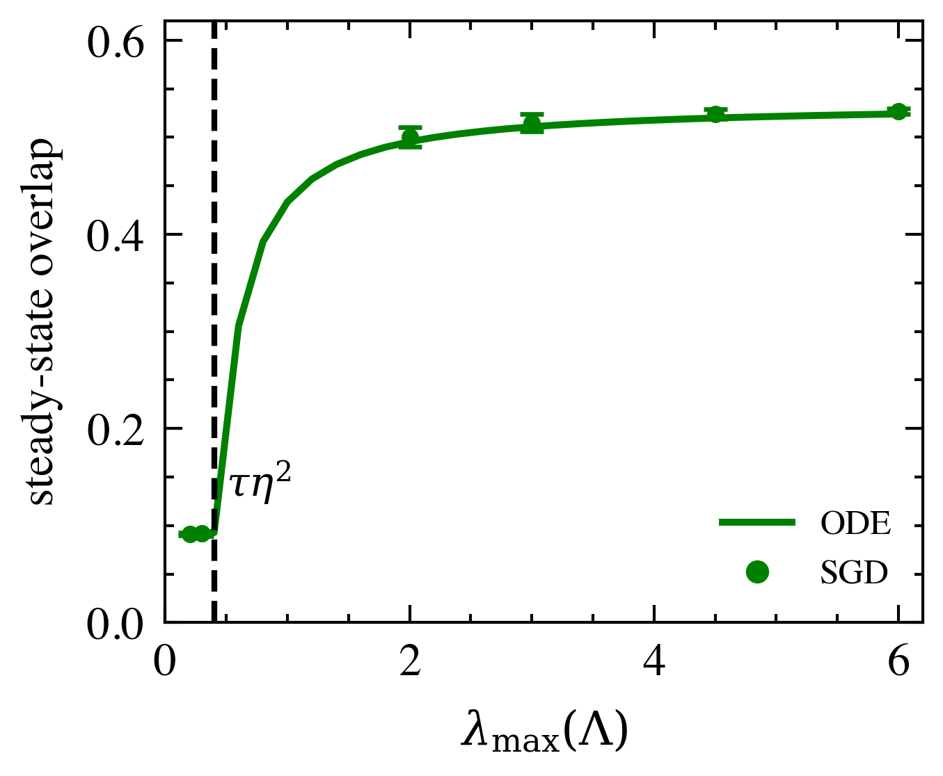
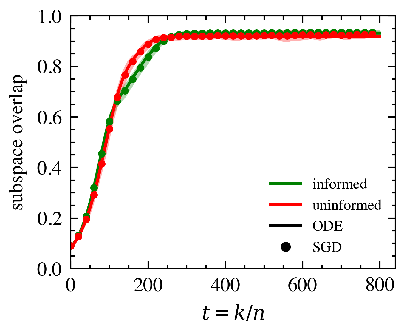
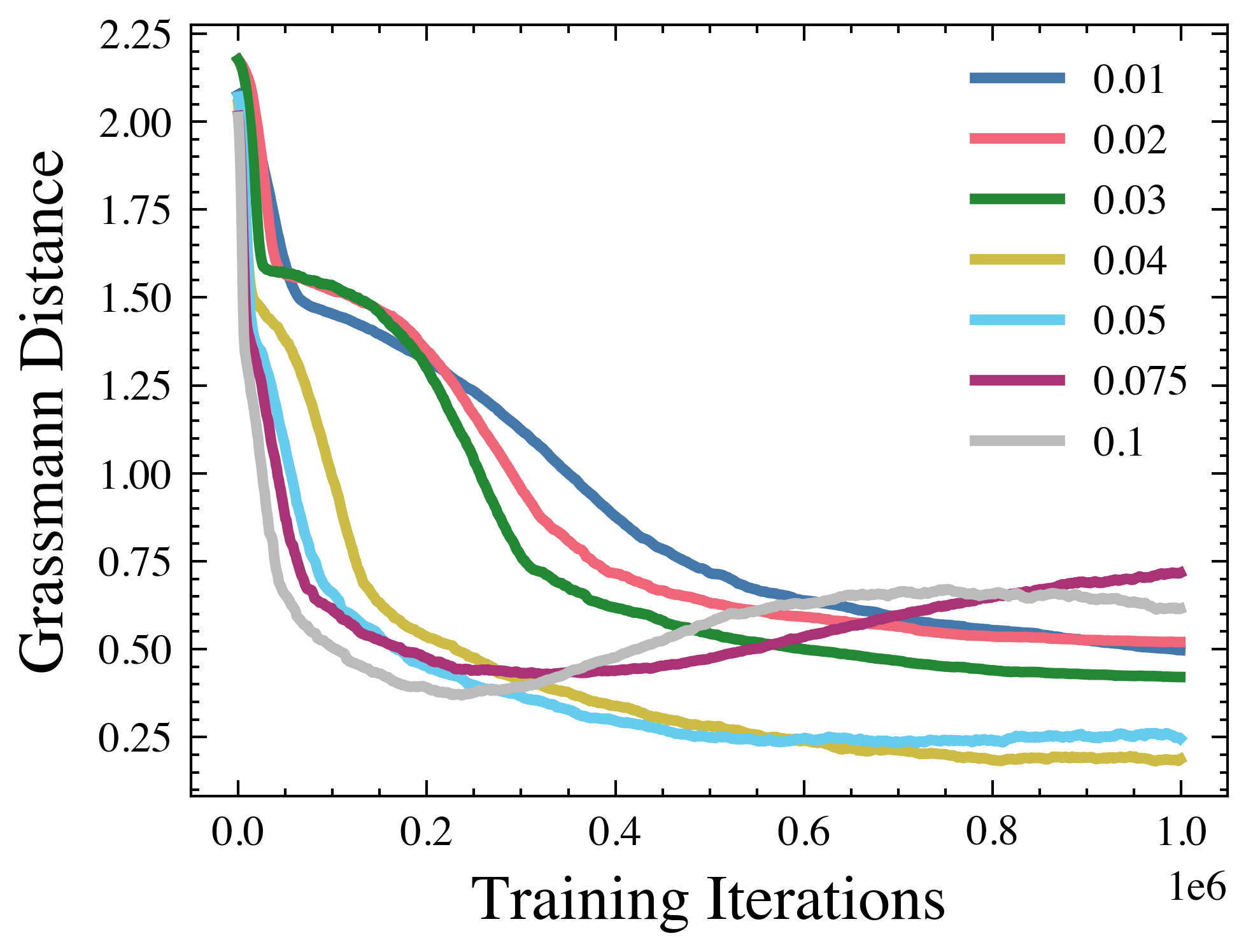
Figure 1: Validation of the theory. Left and middle panels report averages over 10 random seeds with \(3\sigma\) error bars. Left: Signal boosting (Proposition 3): steady-state overlap as a function of \(\lambda_{\max}(\boldsymbol{\Lambda})\) for \(\boldsymbol{\Lambda}=0.2\mathbf{I}+\theta\boldsymbol{\gamma}\boldsymbol{\gamma}^{\top}\). Below the threshold \(\tau\eta^2\) (dashed), recovery fails; once correlation lifts \(\lambda_{\max}\) above this threshold, the boosted direction becomes learnable. Middle: Informed generator covariance (\(\bar{\tilde{\boldsymbol{\Lambda}}}=\boldsymbol{\Lambda}\)) versus uninformed covariance (isotropic with equal total energy) for \(\boldsymbol{\Lambda}=\operatorname{diag}(2,4)\). Informed covariance yields a higher steady-state overlap. In both panels, the ODE prediction (solid) closely tracks high-dimensional SGD (dots). Right: Conditional model with effective eigenvalues \((1,10.8)\) and varying generator learning rate \(\tilde{\tau}\). The transition from convergence to divergence occurs near the predicted boundary \(\tilde{\tau}_{\max}\approx0.046\)..
7.1.1 ODE vs. SGD Dynamics: Signal Boosting and Informed Covariance↩︎
Figure 1 (a) demonstrates signal boosting. The effective covariance is \(\boldsymbol{\Lambda}=0.2\mathbf{I}+\theta\boldsymbol{\gamma}\boldsymbol{\gamma}^\top\), and varying \(\theta\) changes \(\lambda_{\max}(\boldsymbol{\Lambda})\). Below the threshold \(\tau\eta^2\), the steady-state overlap remains near zero. Once the low-rank correlation lifts \(\lambda_{\max}\) above the threshold, the boosted direction becomes recoverable. The SGD points match the ODE curves.
Figure 1 (b) compares informed and uninformed generator covariance for \(\boldsymbol{\Lambda}=\operatorname{diag}(2,4)\). The informed generator uses \(\bar{\tilde{\boldsymbol{\Lambda}}}=\boldsymbol{\Lambda}\), while the uninformed generator uses an isotropic covariance with the same total energy. The informed spectrum reaches a higher steady-state overlap, illustrating that the generator covariance affects the limiting subspace rather than only the convergence rate.
7.1.2 Conditional Model and Stability Boundary↩︎
Figure 1 (c) validates the conditional model and stability boundary on a two-class setup with \(L=2\) and \(d=2\). Class 1 has probability \(0.3\) and strengths \((1,1)\); class 2 has probability \(0.7\) and strengths \((1,15)\), yielding effective covariance \(\bar{\boldsymbol{\Lambda}}=\operatorname{diag}(1,10.8)\). With \(\tau=0.5\), \(\eta=1\), and varying \(\tilde{\tau}\in[0.01,0.1]\), the solvable-region condition predicts a maximal admissible generator learning rate above which the strong mode destabilizes recovery. We track the Grassmann distance \(d(\mathbf{U},\mathbf{V})=(\sum_i\theta_i^2)^{1/2}\), where \(\theta_i\) are principal angles. The empirical transition near \(\tilde{\tau}_{\max}\approx0.046\) matches the prediction.
7.2 Image Experiments: Informed and Uninformed Feature Strengths↩︎
![Figure 2: Informed vs. uninformed feature strengths across three datasets. Grassmann distance between the learned generator subspace and the top-d PCA reference subspace during training (d=64), for MNIST, FashionMNIST, and CIFAR-10 (grayscale). Informed strengths set the generator covariance to the per-class PCA spectrum; uninformed strengths use values sampled uniformly from [0.5,5]. Informed models converge more slowly but reach a lower steady-state distance, while uninformed models converge quickly to a biased plateau.](/article/2606.27246/grassmann_3data.png "fig:")
We next test whether the generator covariance predicted by the theory matters on real image datasets. Since the true low-dimensional subspace is unknown, we use the top-\(d\) PCA subspace of the dataset as a reference and measure the Grassmann distance between this reference and the learned generator subspace. This is not a claim of access to a ground-truth \(\mathbf{U}\); rather, it provides a consistent data-driven comparison across runs.
For MNIST [22], FashionMNIST [23], and CIFAR-10 [24], we compare two generator choices. The informed model sets the generator covariance to the per-class PCA spectrum. The uninformed model uses strengths sampled uniformly from \([0.5,5]\). Figure 2 shows a consistent pattern: informed strengths converge more slowly but reach a lower steady-state Grassmann distance, whereas uninformed strengths converge faster but saturate at a biased plateau. This supports the ODE prediction that \(\bar{\tilde{\boldsymbol{\Lambda}}}\) influences the limiting subspace.
Figure 3 shows samples from the informed conditional model. For each dataset, samples are drawn from the per-class latent distribution and mapped through the shared learned basis \(\mathbf{V}\). Despite the linear generator, the samples are recognizable and class structured, indicating that matching the conditional covariance is important for perceptually coherent generation in this solvable model. In CIFAR-10 case, we do not get sharp images due to the data complexity and limitations of a linear model.


Figure 3: Class-conditional samples from the informed conditional model (MNIST, FashionMNIST, CIFAR-10). For each dataset, the generator covariance is set per class to the data’s PCA spectrum, and samples are drawn from the per-class latent distribution \(\mathcal{N}(\tilde{\mathbf{m}}_\ell,\tilde{\boldsymbol{\Lambda}}_\ell)\) through the shared learned basis \(\mathbf{V}\). Rows correspond to classes and columns to samples..
8 Discussion and Conclusion↩︎
We developed a high-dimensional theory for multi-feature solvable GANs trained on data with conditional, correlated, and non-zero-mean latent structure. The main result is an effective-covariance reduction: for the quadratic energy discriminator, heterogeneous latent structure enters the macroscopic dynamics only through the second moments \(\bar{\boldsymbol{\Lambda}}=\mathbb{E}[\mathbf{c}\mathbf{c}^{\top}]\) and \(\bar{\tilde{\boldsymbol{\Lambda}}}=\mathbb{E}[\tilde{\mathbf{c}}\tilde{\mathbf{c}}^{\top}]\). This yields a deterministic ODE description of the high-dimensional training process and extends solvable GAN dynamics beyond the diagonal unconditional setting.
The stability analysis shows that learnability is governed by the spectrum of the effective covariance. A mode must be strong enough to escape the failure fixed point but not so strong that it destabilizes recovery. Consequently, low-rank correlations can either help or hurt: moderate correlations lift weak directions above the learnability threshold, whereas excessive correlations push the leading eigenvalue beyond the stable-recovery boundary. Numerical simulations validate the ODE, the predicted phase boundary, and this signal-boosting mechanism.
Our experiments further show that the generator covariance is a decisive modeling choice. On MNIST, FashionMNIST, and CIFAR-10, informed conditional feature strengths align the learned generator subspace more closely with the PCA reference subspace and produce coherent class-conditional samples, while uninformed strengths converge faster but saturate at a biased plateau.
The model is intentionally linear and single-layer, which is precisely what makes the training trajectory exactly solvable. Within this tractable setting, the analysis isolates how structured covariance reshapes adversarial subspace learning. Extending the effective-covariance reduction and signal-boosting mechanism to deeper nonlinear generators is a natural direction for future work.
This work was supported by TÜBİTAK 2232 Program (No. 118C337) and project 124E063, and by the KUIS AI Research Center.
Statements and Declarations↩︎
Funding: see Acknowledgements. Competing interests: none. Data availability: all datasets used (MNIST, FashionMNIST, CIFAR-10) are publicly available.
9 Details of the Stability Analysis↩︎
9.1 Fixed Points for the General Case↩︎
We verify that both \(\mathbf{P}=\mathbf{I},\,\mathbf{Q}=\mathbf{R}=0\) and \(\mathbf{P}=\mathbf{Q}=\mathbf{R}=0\) remain fixed points under the generalized effective-covariance model. Setting all derivatives in the macroscopic ODE to zero gives \[\begin{align} 0 &= \tilde{\tau}\bigl( \mathbf{Q}_t \mathbf{R}_t^\top \bar{\tilde{\boldsymbol{\Lambda}}} + \mathbf{P}_t \mathbf{L}_t \bigr), \qquad 0 = \tau\bigl( \bar{\boldsymbol{\Lambda}} \mathbf{Q}_t - \mathbf{P}_t \bar{\tilde{\boldsymbol{\Lambda}}} \mathbf{R}_t + \mathbf{H}_t \mathbf{Q}_t \bigr), \\ 0 &= \tau\bigl( \mathbf{P}_t^\top \bar{\boldsymbol{\Lambda}} \mathbf{Q}_t - \mathbf{S}_t \bar{\tilde{\boldsymbol{\Lambda}}} \mathbf{R}_t + \mathbf{H}_t \mathbf{R}_t \bigr) + \tilde{\tau}\bigl( \bar{\tilde{\boldsymbol{\Lambda}}} + \mathbf{L}_t \bigr) \mathbf{R}_t, \\ 0 &= \tilde{\tau}\bigl( \mathbf{R}_t \mathbf{R}_t^\top \bar{\tilde{\boldsymbol{\Lambda}}} + \bar{\tilde{\boldsymbol{\Lambda}}} \mathbf{R}_t \mathbf{R}_t^\top + \mathbf{S}_t \mathbf{L}_t + \mathbf{L}_t \mathbf{S}_t \bigr). \end{align}\] Both configurations have \(\mathbf{Q}=\mathbf{R}=0\), which gives \(\mathbf{L}=0\) and makes every right-hand side vanish; hence both are fixed points.
9.2 Linearization and Stability↩︎
For the closed-form stability analysis in Section 5, take the matched specialization \(\bar{\boldsymbol{\Lambda}}=\bar{\tilde{\boldsymbol{\Lambda}}}=\boldsymbol{\Lambda}\) and \(\eta_T=\eta_G=\eta\). At both fixed points, \(\mathbf{Q}=\mathbf{R}=0\), so \(\mathbf{L}=0\) and \(\mathbf{H}^*=-\tau\eta^2\mathbf{I}\). Perturbing \(\mathbf{P}=\mathbf{P}^*+\delta\mathbf{P}\), \(\mathbf{Q}=\delta\mathbf{Q}\), \(\mathbf{R}=\delta\mathbf{R}\), and \(\mathbf{S}=\mathbf{S}^*+\delta\mathbf{S}\), the \(\delta\mathbf{P}\) and \(\delta\mathbf{S}\) directions are marginal at first order, and stability is governed by \[\frac{d}{dt}\delta\mathbf{Q} = \tau(\boldsymbol{\Lambda}-\tau\eta^2\mathbf{I})\delta\mathbf{Q} - \tau\mathbf{P}^*\boldsymbol{\Lambda}\delta\mathbf{R}, \qquad \frac{d}{dt}\delta\mathbf{R} = \tau(\mathbf{P}^*)^\top\boldsymbol{\Lambda}\delta\mathbf{Q} + \bigl((\tilde{\tau}-\tau)\boldsymbol{\Lambda}-\tau^2\eta^2\mathbf{I}\bigr)\delta\mathbf{R}. \label{eq:linearized95subsystem}\tag{15}\]
Total failure: For \(\mathbf{P}^*=0\), the system decouples with eigenvalues \(\mu_{Q,i}=\tau(\lambda_i-\tau\eta^2)\) and \(\mu_{R,i}=(\tilde{\tau}-\tau)\lambda_i-\tau^2\eta^2\). Thus, for \(\tilde{\tau}<\tau\) and \(\boldsymbol{\Lambda}\succeq0\), the \(R\)-block is stable automatically, and failure is stable iff \(\lambda_{\max}<\tau\eta^2\); learning begins once \(\lambda_{\max}>\tau\eta^2\). Perfect recovery: For \(\mathbf{P}^*=\mathbf{I}\), each eigendirection gives \(J_i=\begin{psmallmatrix} \tau(\lambda_i-\tau\eta^2) & -\tau\lambda_i\\ \tau\lambda_i & (\tilde{\tau}-\tau)\lambda_i-\tau^2\eta^2 \end{psmallmatrix}\). The trace condition gives \(\tilde{\tau}\lambda_i-2\tau^2\eta^2<0\), i.e., \(\lambda_i<2\tau^2\eta^2/\tilde{\tau}\), and the determinant condition holds automatically for \(\tilde{\tau}<4\tau\). Hence recovery is stable when \(\lambda_{\max}<2\tau^2\eta^2/\tilde{\tau}\), yielding 14 .
9.3 Absence of \(\mathbf{R}\neq\mathbf{0}\) equilibria in the two-timescale regime↩︎
The fixed points of Section 5 all lie on the manifold \(\mathbf{Q}=\mathbf{R}=\mathbf{0}\) (perfect recovery and total failure). For completeness we show that, in the two-timescale regime \(\tilde{\tau}\ll\tau\) in which the solvable region is robust, there are no additional equilibria with \(\mathbf{R}\neq\mathbf{0}\)—i.e.no “stalemate” states in which the discriminator remains locked onto a direction the generator also occupies. Thus, we are free in our analysis to assume that \(\boldsymbol{R} = 0\).
9.3.0.1 Reduction to a single mode.
Take \(\bar{\boldsymbol{\Lambda}}=\bar{\tilde{\boldsymbol{\Lambda}}}=\boldsymbol{\Lambda}\) diagonal, \(\eta_G=\eta_T=\eta\), and \(\mathbf{Z}=\mathbf{I}\) as in Section 5. The macroscopic initialization is diagonal (\(\mathbf{P}_0=p_0\mathbf{I}\), \(\mathbf{Q}_0=q_0\mathbf{I}\), \(\mathbf{R}_0=p_0q_0\mathbf{I}\), \(\mathbf{S}_0=\mathbf{I}\)), and one checks directly from ?? that the diagonal subspace is invariant: every right-hand side maps diagonal states to diagonal states (in particular \(\mathbf{L}=-\operatorname{diag}(\mathbf{R}\mathbf{R}^\top\boldsymbol{\Lambda})\) is diagonal, and all products of diagonal matrices are diagonal). Hence the \(d\)-dimensional system decouples into \(d\) independent copies of the scalar system obtained by restricting ?? to one eigendirection. It therefore suffices to analyze a single mode with strength \(\lambda>0\) and macroscopic scalars \((p,q,r,s)\), where \(L=-r^2\lambda\) and \(H=\big(1-\tfrac{\tau\eta}{2}\big)r^2\lambda-\big(1+\tfrac{\tau\eta}{2}\big)q^2\lambda-\tau\eta^2\). The scalar fixed-point equations are \[\begin{align} 0 &= \tilde{\tau}\,r\lambda\,(q-pr), \tag{16}\\ 0 &= \tau\big(\lambda q-p\lambda r+Hq\big), \tag{17}\\ 0 &= \tau\big(p\lambda q-s\lambda r+Hr\big)+\tilde{\tau}(\lambda+L)r, \tag{18}\\ 0 &= 2\tilde{\tau}\,r^2\lambda\,(1-s). \tag{19} \end{align}\]
9.3.0.2 Structure of an \(r\neq0\) equilibrium.
Suppose \(r\neq0\) (and \(\lambda>0\)). Equation 19 forces \(s=1\), and 16 forces \(q=pr\). Substituting \(q=pr\) into 17 gives \(\lambda pr-p\lambda r+Hpr=Hpr=0\), so either \[\boldsymbol{(a)}\;\;p=0\quad(\text{hence } q=0),\qquad\text{or}\qquad \boldsymbol{(b)}\;\;H=0\;\;(p\neq0).\] We treat the two branches in turn and reduce each to an explicit value of \(r^2\); a genuine equilibrium additionally requires \(r^2\in(0,1]\) and (in branch (b)) \(p^2\in[0,1]\), since \(r=\mathbf{V}^\top\mathbf{W}/n\) and \(p=\mathbf{U}^\top\mathbf{V}/n\) are cosines of principal angles between unit-norm columns.
Branch (a) (pure stalemate, \(p=q=0\)). Here \(H=\big(1-\tfrac{\tau\eta}{2}\big)r^2\lambda-\tau\eta^2\). With \(p=q=0\), \(s=1\), equation 18 reads \(\tau(Hr-\lambda r)+\tilde{\tau}(\lambda-r^2\lambda)r=0\); dividing by \(r\) and solving the resulting linear equation in \(r^2\) gives \[r^2=\frac{\tau^2\eta^2+(\tau-\tilde{\tau})\lambda}{\lambda\big(\tau(1-\tfrac{\tau\eta}{2})-\tilde{\tau}\big)}. \label{eq:app95stalemate}\tag{20}\]
Branch (b) (partial alignment, \(H=0\)). Using \(q=pr\), the condition \(H=0\) is \[r^2\lambda\Big[\big(1-\tfrac{\tau\eta}{2}\big)-\big(1+\tfrac{\tau\eta}{2}\big)p^2\Big]=\tau\eta^2, \label{eq:app95H0}\tag{21}\] while 18 with \(q=pr\), \(s=1\), \(H=0\) becomes \(\tau\lambda r(p^2-1)+\tilde{\tau}\lambda r(1-r^2)=0\), i.e. \[r^2=1-\frac{\tau}{\tilde{\tau}}\,(1-p^2). \label{eq:app95align}\tag{22}\]
9.3.0.3 Infeasibility under TTUR.
Assume the two-timescale regime \(\tilde{\tau}\ll\tau\) together with the mild condition \(\tau\eta<2\) (so that \(1-\tfrac{\tau\eta}{2}>0\)); both hold throughout the operating points of Section 7.
Branch (a). The denominator of 20 is \(\lambda\big(\tau(1-\tfrac{\tau\eta}{2})-\tilde{\tau}\big)>0\) and the numerator \(\tau^2\eta^2+(\tau-\tilde{\tau})\lambda>0\), so \(r^2>0\). Admissibility \(r^2\le1\) would require \(\tau^2\eta^2+(\tau-\tilde{\tau})\lambda\le\lambda\big(\tau(1-\tfrac{\tau\eta}{2})-\tilde{\tau}\big)\), i.e. \[\tau^2\eta^2\le\lambda\Big[\tau\big(1-\tfrac{\tau\eta}{2}\big)-\tilde{\tau}-(\tau-\tilde{\tau})\Big] =-\tfrac{\tau^2\eta}{2}\,\lambda<0,\] which is impossible for \(\lambda>0\). Hence \(r^2>1\): branch (a) admits no equilibrium.
Branch (b). Non-negativity of 22 forces \(\tfrac{\tau}{\tilde{\tau}}(1-p^2)\le1\), i.e.\(p^2\ge1-\tilde{\tau}/\tau\). On the other hand the left-hand side of 21 equals the positive number \(\tau\eta^2\) and \(r^2\lambda>0\), so the bracket must be positive, giving \(p^2<\dfrac{1-\tfrac{\tau\eta}{2}}{1+\tfrac{\tau\eta}{2}}=\dfrac{2-\tau\eta}{2+\tau\eta}<1\). These two requirements are incompatible whenever \[1-\frac{\tilde{\tau}}{\tau}\;>\;\frac{2-\tau\eta}{2+\tau\eta}, \qquad\text{equivalently}\qquad \frac{\tilde{\tau}}{\tau}\;<\;\frac{2\,\tau\eta}{2+\tau\eta},\] which is satisfied in the two-timescale regime \(\tilde{\tau}\ll\tau\) (the right-hand side is a fixed positive number, e.g.\(\tfrac{2\tau\eta}{2+\tau\eta}=\tfrac{2}{5}\) at \(\tau\eta=\tfrac12\)). Hence branch (b) also admits no equilibrium.
Proposition 5 (No \(\mathbf{R}\neq\mathbf{0}\) fixed points under TTUR). For \(\tau\eta<2\) and \(\tilde{\tau}/\tau<2\tau\eta/(2+\tau\eta)\), the scalar system 16 –19 has no solution with \(r\neq0\) and \(r^2\in(0,1]\). By the diagonal-sector reduction, the macroscopic ODE ?? therefore has no equilibrium with \(\mathbf{R}\neq\mathbf{0}\) in this regime.
10 Proof of Main Theorem↩︎
This appendix follows the proof of the scaling-limit theorem in [9], [10]; we restate the key ingredients and indicate the modification required by the generalized latent model, deferring the unchanged moment-bound algebra to those references. The proof applies to the conditional/structured data model because the labels \(l_k\) are sampled i.i.d. and averaged inside the conditional expectations. Consequently, the covariance appearing in the drift is the population effective covariance \(\bar{\boldsymbol{\Lambda}}=\mathbb{E}[\mathbf{c}_k\mathbf{c}_k^\top]\), and likewise \(\bar{\tilde{\boldsymbol{\Lambda}}}\) for the generator. The argument relies on the following stochastic-approximation result from [25].
Lemma 1. Consider a sequence of stochastic processes \(\{\mathbf{x}_k^{(n)}, k=0,1,\dots,\lfloor nT\rfloor\}_{n\ge1}\) for fixed \(T>0\). Suppose \[\mathbf{x}_{k+1}^{(n)}-\mathbf{x}_k^{(n)} = \frac{1}{n}\phi(\mathbf{x}_k^{(n)}) + \boldsymbol{\rho}_k^{(n)} + \boldsymbol{\delta}_k^{(n)},\] where
\(\sum_{k'=0}^k\boldsymbol{\rho}_{k'}^{(n)}\) is a martingale and \(\mathbb{E}\|\boldsymbol{\rho}_k^{(n)}\|^2\le C(T)/n^{1+\epsilon_1}\) for some \(\epsilon_1>0\);
\(\mathbb{E}\|\boldsymbol{\delta}_k^{(n)}\|\le C(T)/n^{1+\epsilon_2}\) for some \(\epsilon_2>0\);
\(\phi\) is Lipschitz;
\(\mathbb{E}\|\mathbf{x}_k^{(n)}\|^2\le C\) for all \(k\le\lfloor nT\rfloor\);
\(\mathbb{E}\|\mathbf{x}_0^{(n)}-\mathbf{x}_0^*\|\le C/n^{\epsilon_3}\) for some \(\epsilon_3>0\) and deterministic \(\mathbf{x}_0^*\).
Then \(\|\mathbf{x}_k^{(n)}-\mathbf{x}(k/n)\|\le C(T)n^{-\min(\epsilon_1/2,\epsilon_2,\epsilon_3)}\), where \(\mathbf{x}(t)\) is the unique solution of \(\frac{d}{dt}\mathbf{x}(t)=\phi(\mathbf{x}(t))\) with \(\mathbf{x}(0)=\mathbf{x}_0^*\).
10.0.0.1 Application to the macroscopic state.
We apply Lemma 1 to \(\mathbf{M}_k\), with \[\label{eq:M95decomposition} \mathbf{M}_{k+1}-\mathbf{M}_k = \frac{1}{n}\phi(\mathbf{M}_k) + \underbrace{\bigl(\mathbf{M}_{k+1}-\mathbb{E}_k\mathbf{M}_{k+1}\bigr)}_{\boldsymbol{\rho}_k^{(n)}} + \underbrace{\bigl[\mathbb{E}_k\mathbf{M}_{k+1}-\mathbf{M}_k-\tfrac{1}{n}\phi(\mathbf{M}_k)\bigr]}_{\boldsymbol{\delta}_k^{(n)}},\tag{23}\] where \(\phi\) is the right-hand side of ?? . Conditions (C.3) and (C.5) follow from assumptions (A.3) and (A.5). The martingale and moment estimates required for (C.1), (C.2), and (C.4) are the same as in [9], [10], using (A.6) to control the discriminator block.
10.0.0.2 Where the effective covariance enters.
The latent distribution appears in the drift through expectations of quadratic latent terms. Averaging the generator and discriminator updates over latent variables, noise, and conditional labels gives \[\mathbb{E}_k\mathbf{P}_{k+1}-\mathbf{P}_k = \frac{\tilde{\tau}}{n} \bigl[\mathbf{Q}_k\mathbf{R}_k^\top\bar{\tilde{\boldsymbol{\Lambda}}}+\mathbf{P}_k\mathbf{L}_k\bigr], \quad \mathbb{E}_k\mathbf{Q}_{k+1}-\mathbf{Q}_k = \frac{\tau}{n} \bigl[\bar{\boldsymbol{\Lambda}}\mathbf{Q}_k-\mathbf{P}_k\bar{\tilde{\boldsymbol{\Lambda}}}\mathbf{R}_k+\mathbf{H}_k\mathbf{Q}_k\bigr].\] The remaining \(\mathbf{R}_k\) and \(\mathbf{S}_k\) drift terms are obtained analogously. Thus, the only change from the unconditional proof is the replacement of \((\boldsymbol{\Lambda},\tilde{\boldsymbol{\Lambda}})\) by \((\bar{\boldsymbol{\Lambda}},\bar{\tilde{\boldsymbol{\Lambda}}})\).
Conclusion. With (C.1)–(C.5) verified, Lemma 1 applies to the macroscopic process \(\mathbf{M}_k\), proving Theorem 1.