Abstract. We construct explicit approximations to the solution of a second-order parabolic partial differential equation on the real line with variable coefficients. The method is based on Chernoff’s product formula and uses a new operator-valued function defined through proper Riemann integrals over a bounded interval, which makes the approach readily usable in numerical practice. For sufficiently smooth initial data and coefficients, we prove that the resulting Chernoff approximations converge uniformly in space and time with a quadratic rate, improving the standard first-order estimate. The construction yields a new class of quasi-Feynman formulas that are neither grid-based nor Galerkin-type, but instead rely on semigroup theory and multiple bounded integrals. The theoretical findings are validated by symbolic computation, and the paper contributes both refined error bounds and a practical analytical tool for parabolic problems.

Keywords: Cauchy problem for parabolic PDE, approximation of solution, rate of convergence to the solution, multiple proper Riemann integral, one-parameter semigroup of operators, Chernoff product formula

MSC2020: primary 65M15, secondary 47D06, 35K15

1 Introduction↩︎

Theory and practice of solving partial differential equations (PDEs) numerically is an old branch of applied mathematics. Finding solution with appropriate accuracy is extremely important in almost all areas of advanced contemporary engineering, experimental and theoretical physics and chemistry, in particular, in construction of materials, projecting of buildings and devices. The literature on this topic is abundant: almost every large publishing house has in its portfolio a book called Numerical methods for partial differential equations, see [1]–[4]. All this abundance grows from the fact that it is difficult and important to solve partial differential equations, and there is no numerical method which is applicable to all useful equations. This is why research in this direction is far from ending.

This paper is devoted to derivation of a formula that expresses arbitrary accurate approximations to solution of PDE with variable coefficients explicitly in terms of these coefficients that play a role of parameters in the problem. This can be considered as a new method for solving parabolic PDEs with variable coefficients.

At the present time we know of a relatively small number of situations where a short formula expresses the solution of a partial differential equation with variable coefficients in terms of these coefficients and initial/boundary conditions. However, with the use of Chernoff’s theorem (see original paper by Paul Chernoff [5], textbook [6] or Theorem 2 below) it is possible to write such formulas for approximations to the solution. This fact gives a birth to a new branch of numerical methods which are neither grid-based, nor Galerkin, nor Monte-Carlo, nor iterative, but something in between and at the same time something apart, with the rich flavour of functional analysis. There is a very good recent overview [7] describing the results and history of the method of Chernoff approximations.

Employing this method we construct a sequence of functions (Chernoff approximations) which converges (uniformly in \(x\in\mathbb{R}\), \(t\in[0,t_0]\) for arbitrary \(t_0>0\)) to the exact solution of the Cauchy problem for diffusion-type second order parabolic equation given by \[\label{firsteq} \left\{ \begin{array}{ll} u'_{t}(t,x)=a(x)u_{xx}''(t,x)+b(x)u'_x(t,x) +c(x)u(t,x)\stackrel{denote}{=}(Hu(t,\cdot))(x), \\ u(0,x)=u_0(x). \end{array} \right.\tag{1}\]

Where \(x\in\mathbb{R}\), \(t\geq0\), \(u\colon [0,+\infty)\times \mathbb{R}\to \mathbb{R}\), and functions \(a,b,c,u_0\colon\mathbb{R}\to\mathbb{R}\) are bounded and uniformly continuous. We also assume that \(a(x)>a_0\equiv\mathrm{const}>0\) for all \(x\in\mathbb{R}\), and first and second derivatives of \(a,b,c\) are bounded and uniformly continuous as functions \(\mathbb{R}\to\mathbb{R}\).

This paper is dedicated to deriving formulas presented in Theorem 4 and Theorem 5 that give the solution of (1 ) in terms of \(a\), \(b\), \(c\), \(u_0\) assuming that the second order differential operator \(H\) is an infinitesimal generator of the \(C_0\)-semigroup \(\left(e^{tH}\right)_{t\geq 0}\) (later we will explain meaning of these words in the Preliminaries section). This assumption is a standard case in studies of class of evolution equations that the examined equation (1 ) belongs to. According to general theory of \(C_0\)-semigroups [6] this assumption implies that the solution of the Cauchy problem (1 ) exists, is bounded and uniformly continuous with respect to \(x\) for each \(t\), depends on \(u_0\) continuously, and can be represented in a form \(u(t,x)=\left(e^{tH}u_0\right)(x)\), we will discuss this in more words below in Theorem 1. The last equality means that if one knows \(e^{tH}\) for each \(t>0\) then (1 ) is solved (in the appropriate sense) for each \(u_0\). We apply the Chernoff theorem to a specially constructed family of linear bounded operators \((S(t))_{t\geq 0}\) defined as proper Riemann integrals of functions containing \(a\), \(b\), \(c\). This allows us to express \(e^{tH}\) in terms of \(a\), \(b\), \(c\), reaching the proposed goal. The aim of the paper do not include detailed discussion of the problem of finding the class of functions in which the solution to (1 ) is unique under certain assumptions on functions \(a\), \(b\), \(c\), \(u_0\), but we keep in mind that for the heat equation there are known unbounded solutions. To have high speed of convergence of our approximations we ask additionally that initial condition \(u_0\) has bounded uniformly continuous derivatives up to order 8, and coefficients \(a,b,c\) have bounded uniformly continuous derivatives up to order 6.

For (1 ) there are known Chernoff approximations for the solution in terms of shift operators [8], [9] and in terms of improper Riemann integral operators [10] but they are difficult to use in practice, meanwhile our approximations are better designed for real-world applications.

An important question is how fast the error decreases in the approximation expression \(e^{tH}u_0\approx S(t/n)^nu_0\) provided by the Chernoff theorem as \(n\) tends to infinity. For a particular case of Schrödinger equation this question was discussed in [11], but generally this issue is not well developed at the present moment. It was mentioned in [12] that the speed of convergence depends sufficiently on the initial condition, and for some semigroups there are Chernoff functions providing arbitrary slow convergence of approximations. The notion of approximation subspace was proposed in [12] to study this issue, and some numerical experiments were performed recently in [13]–[15].

There is a recent improvement [16] in direction of research where the convergence \(S(t/n)^n\to e^{tH}\) as \(n\to \infty\) is studied in operator norm hence convergence \(S(t/n)^nu_0\to e^{tH}u_0\) as \(n\to \infty\) is uniform with respect to initial condition \(u_0\) from unit sphere in \(\mathcal{F}\), but examples from [12], [13], [17], [18] show that only convergence \(S(t/n)^nu_0\to e^{tH}u_0\) as \(n\to \infty\) on each vector \(u_0\) is what we should expect in general case. However, in [17], [18] conditions were found that provide estimate from above on the norm of approximation error that appears in the Chernoff theorem. We will use results of [17], [18] as one of the technical tools, see Theorem 3.

See also research [19]–[21] (and references therein) in a more general setting than Chernoff’s theorem. The same question arises for the Trotter product formula \(e^{A+B}=\lim_{n\to\infty}(e^{A/n}e^{B/n})^n\) which we do not use but which is a particular case of Chernoff’s theorem for operator-valued Chernoff function \(G(t)=e^{tA}e^{tB}\), see [22]–[24].

The main result of the present paper is Theorem 5.

2 Preliminaries↩︎

We employ extensively the language and methods of functional analysis and \(C_0\)-semigroup theory, information on these topics can be found e.g. in classical textbooks [6], [25], [26]. This list is not exhaustive but each of these books is sufficient to understand well all the contents of the paper. Nevertheless, in this section we recall some basic definitions and facts to fix the notation, make the paper self-contained, and highlight the ideas that we will use. All information that is given in Preliminaries section without references is available in [6], [25], [26], the best choice is probably [6].

2.1 \(C_0\)-semigroups↩︎

Let \(\mathcal{F}\) be a real Banach space. Let \(\mathscr{L}(\mathcal{F})\) be a set of all bounded linear operators in \(\mathcal{F}\). Suppose we have a mapping \(V\colon [0,+\infty)\to \mathscr{L}(\mathcal{F}),\) i.e., \(V(t)\) is a bounded linear operator \(V(t)\colon \mathcal{F}\to \mathcal{F}\) for each \(t\geq 0.\) The mapping \(V\) is called a \(C_0\)-semigroup, or a strongly continuous one-parameter semigroup of operators, if it satisfies the following conditions:

1) \(V(0)\) is the identity operator \(I\), i.e., for each \(\varphi\in \mathcal{F}\) we have \(V(0)\varphi=\varphi;\)

2) \(V\) maps the addition of numbers in \([0,+\infty)\) into a composition of operators in \(\mathscr{L}(\mathcal{F})\), i.e., for all \(t\geq 0\) and all \(s\geq 0\) we have \(V(t+s)=V(t)\circ V(s),\) where \((A\circ B)(\varphi)=A(B(\varphi))=AB\varphi\);

3) \(V\) is continuous with respect to the strong operator topology in \(\mathscr{L}(\mathcal{F})\), i.e., for all \(\varphi\in \mathcal{F}\) function \(t\longmapsto V(t)\varphi\) is continuous as a mapping from \([0,+\infty)\) to \(\mathcal{F}.\)

It is known that if \((V(t))_{t\geq 0}\) is a \(C_0\)-semigroup in Banach space \(\mathcal{F}\) then the set \[\left\{\varphi\in \mathcal{F}: \exists \lim_{t\to +0}\frac{V(t)\varphi-\varphi}{t}\right\}\stackrel{denote}{=}D(L)\] is a dense linear subspace in \(\mathcal{F}\). The operator \(L\) defined on the domain \(D(L)\) by the equality \[L\varphi=\lim_{t\to +0}\frac{V(t)\varphi-\varphi}{t}\] is called an infinitesimal generator (or just generator for short) of the \(C_0\)-semigroup \((V(t))_{t\geq 0}\). The generator \((L,D(L))\) is a closed linear operator that defines the \(C_0\)-semigroup \((V(t))_{t\geq 0}\) uniquely, and notation \(V(t)=e^{tL}\) is used. If \(L\) is a bounded operator and \(D(L)=\mathcal{F}\), then \(e^{tL}\) is indeed the exponent defined by the power series \(e^{tL}=\sum_{k=0}^\infty\frac{t^kL^k}{k!}\) converging with respect to the norm topology in \(\mathscr{L}(\mathcal{F})\). In most interesting cases the generator is an unbounded differential operator, e.g., Laplacian \(\Delta\) is the generator of a multidimensional heat semigroup, and operator \(H\) is the generator of semigroup providing solutions to (1 ) in the sense that will be explained below.

2.2 Abstract Cauchy problem for evolution equation in Banach space↩︎

One of the reasons for the study of \(C_0\)-semigroups is their connection with differential equations. We will start from the so-called abstract Cauchy problem (2 ) and then explain how it is related to (1 ). Consider Banach space \(\mathcal{F}\), vector \(u_0\in\mathcal{F}\), linear operator \(L\colon D(L)\to\mathcal{F}\) with domain \(D(L)\subset\mathcal{F}\), and state the following abstract Cauchy problem: find function \(U\colon [0,+\infty)\to\mathcal{F}\) such that \[\label{aCp} \left\{ \begin{array}{ll} U'(t)=LU(t) \;\mathrm{ for }\;t\geq 0,\\ U(0)=u_0. \end{array} \right.\tag{2}\]

Equality \(U'(t)=LU(t)\) is called linear evolution equation in \(\mathcal{F}\) with operator \(L\). Function \(U\) is called a classical solution to (2 ) iff \(U\) has continuous derivative with respect to norm in \(\mathcal{F}\), \(U(t)\in D(L)\) for all \(t\geq 0\) and (2 ) holds. Function \(U\) is called a mild solution to (2 ) iff \(U\) is continuous with respect to norm in \(\mathcal{F}\), and for all \(t\geq 0\) we have \(\int\limits_0^tU(s)ds\in D(L)\) and \(U(t)=u_0+L\int\limits_0^tU(s)ds\).

In elementary example provided by one-dimensional Banach space \(\mathcal{F}=\mathbb{R}\) we have \(D(L)=\mathbb{R}\), \(u_0\in\mathbb{R}\), and \(L\) is a real number which also can be considered as an operator of multiplication by \(L\). Then (2 ) is a standard ordinary differential equation which is known to have solution \(U(t)=e^{tL}u_0\) both in mild and classical sense which is easy to check by direct computation. It is beautiful and amazing that in case of infinite-dimensional space \(\mathcal{F}\) this fact holds true (with some technical details added) and even the formula \(U(t)=e^{tL}u_0\) continues to work properly. The following statement gives exact meaning to this emotional comment.

Recall also that \(e^{tL}\) is a linear bounded operator, so for each \(t\geq 0\) solution \(U(t)=e^{tL}u_0\) depends on \(u_0\) linearly and continuously with respect to norm in \(\mathcal{F}\). Now let us explain how initial-value problems similar to (1 ) and even more general are related with (2 ).

2.3 Cauchy problem for partial differential equation (PDE) of evolution type and its connection to abstract Cauchy problem↩︎

In general situation, if \(Q\) is a set (in (1 ) we have \(Q=\mathbb{R}\)), then the function \(u\colon [0,+\infty)\times Q\to \mathbb{R}\), \(u\colon (t,x)\longmapsto u(t,x)\) of two variables \((t,x)\) can be considered as a function \(U\colon t\longmapsto [x\longmapsto u(t,x)]=u(t,\cdot)\) of one variable \(t\) with values in the space of real-valued functions of variable \(x\). Let \(\mathcal{F}\subset\mathbb{R}^Q\) be a space of (not necessarily all) real-valued functions on \(Q\). Suppose that \(\mathcal{F}\) is a Banach space with respect to some appropriate norm, and \((L,D(L))\) is a closed densely defined linear operator in \(\mathcal{F}\). If \(U(t)=u(t,\cdot)\in\mathcal{F}\) for all \(t\geq 0\) then one can define \(Lu(t,x)=(Lu(t,\cdot))(x)=(LU(t))(x).\) With these definitions it is clear that the Cauchy problem \[\label{aCpforPDE} \left\{ \begin{array}{ll} u'_t(t,x)=Lu(t,x) \;\mathrm{ for }\;t\geq 0, x\in Q\\ u(0,x)=u_0(x)\;\mathrm{ for } \;x\in Q \end{array} \right.\tag{3}\] is exactly (2 ) with the only one difference: derivative \(u'_t(t,x)\) in (3 ) above is taken in \(\mathbb{R}\) pointwise for each \(x\in Q\), meanwhile in (2 ) the derivative \(U'(t)\) is taken with respect to norm in \(\mathcal{F}\): \[u'_t(t,x)=p(t,x)\iff \lim_{\varepsilon\to0}\left|\frac{u(t+\varepsilon,x)-u(t,x)}{\varepsilon}-p(t,x)\right|=0\textrm{ for all }x\in Q,\] \[U'(t)=P(t)\iff \lim_{\varepsilon\to0}\left\|\frac{U(t+\varepsilon)-U(t)}{\varepsilon}-P(t)\right\|=0.\]

If there exists a \(C_0\)-semigroup \((e^{tL})_{t\geq 0}\) then thanks to theorem 1 Cauchy problem (2 ) has unique classical solution for each \(u_0\in D(L)\) and unique mild solution for each \(u_0\in\mathcal{F}\). If one selects appropriate definition of solution to (3 ) that meets the above-mentioned difference in understanding the time derivative, then solution to (3 ) is made of solution to (2 ), i.e., function \(u(t,x)=(U(t))(x)=(e^{tL}u_0)(x)\) solves (3 ) in the appropriate sense.

Setting (3 ) is very general because the role of \(L\) can be played, e.g., by arbitrary differential operator with derivatives of any order and coefficients that depend on \(x\) but do not depend on \(t\). This covers the case (1 ) in particular. Also \(L\) may be a pseudo-differential operator. If \(L=-i\mathcal{H}\), where \(\mathcal{H}\) is the Hamiltonian of a quantum system then (3 ) is a Schrödinger equation. Variable \(x\) can run over \(\mathbb{R}\), \(\mathbb{R}^n,\) manifold, ramified surface, infinite-dimensional space or a subset in these spaces, examples can be found in [7].

2.4 Assumptions and notation that we use↩︎

Now it is time to introduce the case which we study in the paper. In our consideration \(Q=\mathbb{R}\), and \(\mathcal{F}=UC_b(\mathbb{R})\) is the space of all bounded and uniformly continuous real-valued functions that are defined on \(\mathbb{R}\). We consider \(\mathcal{F}=UC_b(\mathbb{R})\) with the uniform norm \(\|f\|=\sup_{x\in\mathbb{R}}|f(x)|\). It is easy to check that \(UC_b(\mathbb{R})\) is a closed subset of the space \(C_b(\mathbb{R})\) of all bounded real-valued functions defined on \(\mathbb{R}\). It is a standard fact that \(C_b(\mathbb{R})\) is a Banach space with respect to uniform norm, so our \(\mathcal{F}=UC_b(\mathbb{R})\) is also a Banach space. We also will use notation \[UC_b^n(\mathbb{R})=\{f\in UC_b(\mathbb{R})\;|\;f',f'',\dots,f^{(n)}\in UC_b(\mathbb{R})\}\subset\mathcal{F}=UC_b(\mathbb{R})\textrm{ and } C_b^\infty(\mathbb{R})=\bigcap\limits_{n=1}^\infty UC_b^n(\mathbb{R}).\] It is proved in [9] that \(C_b^\infty(\mathbb{R})\) is dense in \(UC_b(\mathbb{R})\). In our consideration \(L=H\), i.e., \[(Lf)(x)=(Hf)(x)=a(x)f''(x)+b(x)f'(x)+c(x)f(x)\] for each point \(x\in\mathbb{R}\) and each function \(f\in UC_b^\infty(\mathbb{R})\). The domain \(D(L)=D(H)\) is defined via the following assumption.

Assumption 1. We assume that operator \(H\) defined above on the set \(C_b^\infty(\mathbb{R})\) is closable and its closure \((H,D(H))\) generates a \(C_0\)-semigroup \((e^{tH})_{t\geq 0}\) in \(\mathcal{F}=UC_b(\mathbb{R})\) endowed with the uniform norm \(\|f\|=\sup_{x\in\mathbb{R}}|f(x)|\). In other words: \((H,D(H))\) is a closed linear operator that generates a \(C_0\)-semigroup, and \(C_b^\infty(\mathbb{R})\) is a core for \((H,D(H))\).

This assumption is a condition on properties of function \(a,b,c\) and usually is not very restrictive. For example, it holds for the case \(a(x)\equiv 1, b(x)\equiv c(x)\equiv 0\) when (1 ) is the heat equation. Also it holds if \(a,b,c\in C_b^\infty(\mathbb{R})\) and there exists such \(\varepsilon_0>0\) that \(a(x)\geq\varepsilon_0\) for all \(x\in\mathbb{R}\). We will use Theorem 3 which also states that Assumption 1 holds for the case that we study.

Domain of the operator which is a closure of some other operator is usually difficult to express explicitly, but at least we know that \(C_b^\infty(\mathbb{R})\subset D(L)\). In practice of solving (1 ) the set \(D(L)\) is not important because the solution to (1 ) is given by \(u(t,x)=(e^{tL}u_0)(x)\), and, independently of how big the set \(D(L)\) is, \(e^{tL}\) is a linear bounded operator defined everywhere on \(\mathcal{F}\). So, with the use of Theorem 1, we see that important thing is that \(C_0\)-semigroup \((e^{tL})_{t\geq 0}\) exists because it gives the solution to (2 ) hence the solution to (1 ).

The last thing that we need to discuss here is the time derivative. Suppose that \(U(t)\) is the mild or the classical solution of (1 ) in \(\mathcal{F}=UC_b(\mathbb{R})\); what does this mean for \(u\) defined as \(u(t,x)=(U(t))(x)\)? For the mild solution of (1 ) it is required that \(U(t)\) is continuous in \(t\), which means that \(u(t,x)\) is continuous in \(t\) uniformly with respect to \(x\in\mathbb{R}\). Also \(U(t)=u(t,\cdot)\in\mathcal{F}\) which means that \(u(t,x)\) is bounded and uniformly continuous in \(x\) for each \(t\geq 0\). Condition \(U(t)=u_0+H\int\limits_0^tU(s)ds\) means that the integral \(\int\limits_0^tu(s,x)ds\) exists uniformly with respect to \(x\in\mathbb{R}\) and \([x\longmapsto \int\limits_0^tu(s,x)ds]\in D(H)\) where \(D(H)\) is defined in the Assumption 1.

Suppose now that \(U(t)\) is the classical solution of (1 ). Suppose that we have some function \(p(t)\in\mathcal{F}\), i.e. \(p(t,x)\) is bounded and uniformly continuous in \(x\) for each \(t\geq 0\), and \(p(t)=U'(t)\). This means that \(0=\lim_{\varepsilon\to0}\left\|\frac{U(t+\varepsilon)-U(t)}{\varepsilon}-p(t)\right\|=\lim_{\varepsilon\to0}\sup_{x\in\mathbb{R}}\left|\frac{u(t+\varepsilon,x)-u(t,x)}{\varepsilon}-p(t,x)\right|\), so \((U'(t))(x)=u'_t(t,x)=p(t,x)\) exists for each fixed \(x\in\mathbb{R}\), and, moreover function \(u'_t(t,x)\) is bounded and uniformly continuous in \(x\) for each \(t\geq 0\). The limit expression above means exactly that \(u(t,x)\) is differentiable in \(t\) uniformly in \(x\in\mathbb{R}\). Finally, it follows from the definition of a classical solution, that \(U'(t)\) is continuous with respect to the norm in \(\mathcal{F}\), so for each \(t\geq 0\) we have \(0=\lim_{\varepsilon\to0}\|U'(t+\varepsilon)-U'(t)\|=\lim_{\varepsilon\to0}\sup_{x\in\mathbb{R}}|u'_t(t+\varepsilon,x)-u'_t(t,x)|\) which means exactly that \(u_t'(t,x)\) is continuous in \(t\) uniformly in \(x\in\mathbb{R}\) for each \(t\geq 0\).

Now we have introduced everything which is needed to define the solution of (1 ) which we are eager to find approximately via Chernoff approximations.

2.5 Setting of the problem that is solved in the paper↩︎

Problem 1. For the Cauchy problem (1 ) \[\left\{ \begin{array}{ll} u'_{t}(t,x)=a(x)u_{xx}''(t,x)+b(x)u'_x(t,x) +c(x)u(t,x)\stackrel{denoted}{=}(Hu(t,\cdot))(x), \\ u(0,x)=u_0(x). \end{array} \right.\] we wish to find (approximately with estimates on the approximation error):

1. Mild solution, i.e. function \(u(t,x)\) which for each \(t\geq 0\) is: bounded, uniformly continuous in \(x\), continuous in \(t\) uniformly with respect to \(x\in\mathbb{R}\), and satisfies \(u(t,x)=u_0(x)+\left(a(x)\frac{\partial^2}{\partial x^2}+b(x)\frac{\partial}{\partial x}+c(x)\right)\int\limits_0^tu(s,x)ds\) where the integral exists uniformly with respect to \(x\in\mathbb{R}\), and \([x\longmapsto \int\limits_0^tu(s,x)ds]\in D(H)\) where \(D(H)\) is defined in the Assumption 1.

2. Classical solution, i.e. function \(u(t,x)\) which for each \(t\geq 0\) is: bounded, uniformly continuous in \(x\), continuous and differentiable in \(t\) uniformly with respect to \(x\in\mathbb{R}\). Moreover \(u_t'(t,x)\) is continuous in \(t\) for each \(t\geq 0\) uniformly with respect to \(x\in\mathbb{R}\), \([x\longmapsto u(t,x)]\in D(H)\) where \(D(H)\) is defined in the Assumption 1, and \(u'_t(t,x)=\left(a(x)\frac{\partial^2}{\partial x^2}+b(x)\frac{\partial}{\partial x}+c(x)\right)u(t,x)dx\) holds.

Comment on the problem. Both solutions mentioned in items 1 and 2 above are given by the formula \(u(t,x)=(e^{tH}u_0)(x)\) thanks to general theory of \(C_0\)-semigroups and introductive considerations made above; see propositions 6.3 and 6.4 in the book [6]. So Problem 1 is reduced to problem of approximating of \(e^{tH}\) with controlled approximation error. The key instrument for doing this is Theorem 3.

What do we do to solve this problem. In terms of linear bounded operators \(S(t)\) introduced in Theorem 5 below, we will construct a sequence of functions \(u_n(t,x)=(S(t/n)^nu_0)(x)\) which for each \(t\geq 0\) and each \(n=1,2,3,\dots\) are: bounded, uniformly continuous in \(x\), continuous in \(t\) uniformly with respect to \(x\in\mathbb{R}\). For each \(t_0>0\) sequence \(u_n(t,x)\) satisfies \[\lim_{n\to\infty}\sup_{t\in[0,t_0]}\sup_{x\in\mathbb{R}}|u_n(t,x)-u(t,x)|=0\] where \(u(t,x)\) is the classical solution of (1 ) for all \(u_0\in D(H)\), and \(u(t,x)\) is the mild solution of (1 ) for all \(u_0\in UC_b(\mathbb{R})\). Moreover, we prove the following estimate on the rate of convergence: \[\sup_{t\in[0,t_0]}\sup_{x\in\mathbb{R}}|u_n(t,x)-u(t,x)|=O(1/n^2) \textrm{ as } n\to\infty\] at least for all \(u_0\in UC_b^8(\mathbb{R})\) and \(a,b,c\in UC_b^6(\mathbb{R})\) satisfying Assumption 1.

3 Main result↩︎

3.1 Approach proposed (the method of Chernoff approximation)↩︎

To reach the aim of the paper we use the method of Chernoff approximation [7]. Let us explain what it is.

Division of (CT) into (CT0)-(CT1) helps to check these subconditions separately because they are usually proved by methods of different nature. The condition of Chernoff tangency implies that \(G(t)f=f+tLf+o(t)\) as \(t\to 0\) for all \(f\) from the space which is a core for \((L,D(L))\). With the notion of Chernoff tangency the classic Chernoff theorem can be stated in the following form.

If \(G\) is Chernoff-tangent to \(L\), then the expression \(G(t/n)^nf\) is called a Chernoff approximation expression for \(e^{tL}f\), and \(G(t/n)^nu_0\) is called a Chernoff formal solution for Cauchy problem \([U'(t)=LU(t); U(0)=u_0]\). If, moreveover, (?? ) holds, then \(G\) is called a Chernoff function for operator \(L\), and \(G\) is called Chernoff-equivalent to \(C_0\)-semigroup \((e^{tL})_{t\geq 0}\); in this case \(U(t)=\lim_{n\to\infty}G(t/n)^nu_0=e^{tL}u_0\) is the solution of this Cauchy problem due to Theorem 1.

The Chernoff theorem (and definitions derived from it) admit two equivalent wordings: with unbounded time and with arbitrary small time. The first is provided above. The second arises when Chernoff function in (CT) is defined not for all \(t\geq 0\), but only for \(t\in[0,\delta)\) for fixed small \(\delta>0\). The condition \((N)\) in the second case is substituted by the following condition (N’):

(N’) There exists \(\omega_1>0\) such that \(\|G(t)\|\leq 1+\omega_1 t\) for all \(t\in[0,\delta)\).

This wording is motivated by the fact that the value of \(t/n\) in Chernoff approximation expression \(G(t/n)^nf\) becomes arbitrary small as \(n\to\infty\) while \(t\in[0,t_0]\). This is also in line with the condition (CT3) which itself uses \(G(t)\) defined only for small values of \(t>0\).

One may ask why finding Chernoff function for operator \(L\) is simpler than finding \(e^{tL}\) using some other method? Why one should use Chernoff’s theorem? The first reason is that there are no standard methods of finding \(e^{tL}\) for most interesting operators \(L\) with variable coefficients, so usually we can only refer to solving the Cauchy problem (3 ) for each \(u_0\in\mathcal{F}\) or to finding the resolvent of \(L\) which is not an easy task when \(L\) has variable coefficients. The second reason is that Chernoff function \(G\) may not have semigroup composition property, i.e. \(G(t_1+t_2)\) is allowed to be not equal to \(G(t_1)G(t_2)\)), which gives us some freedom in writing the formula for \(G\). With this freedom, sometimes it is possible to define \(G(t)\) by a short formula containing variable coefficients of operator \(L\) as parameters. It is exactly what we do in the paper.

The definition of Chernoff equivalence goes back to 2002’s definiton by O.G. Smolyanov [28], who since 2000’s papers [29]–[31] until his death in 2021 systematically applied Chernoff’s theorem to solving Cauchy problem for linear evolution equations, see overviews [7], [32]. We will use the following result from [17]:

3.2 Derivation of a formula for Chernoff approximations based on S(t)↩︎

Theorem 4 constructs a Chernoff function that does not generate rapidly converging approximations. However, it allows the solution to the Cauchy problem (1 ) for a parabolic differential equation to be represented in the form of a new type of Feynman formula. Specifically, in the formula defining the solution, the integral is not taken over the set traversed by the variable \(x\), i.e., not along the line \(\mathbb{R}\). Instead, the integral is taken over the interval \([-1,1]\), and due to the boundedness of the integrand and the interval of integration, it is a proper Riemann integral. Subsequently, the Chernoff function from Theorem 4 is used in Theorem 5 to create another Chernoff function (which we again denote by symbol \(S\)) that generates rapidly converging Chernoff approximations.

The following Theorem 5 is the main result of the present paper. It proposes Chernoff function \(S(t)\) which provides Chernoff approximations to solutions of (1 ). The solution is given in the form \(u(t,x)=\lim_{n\to\infty}u_n(t,x)\) where Chernoff approximations \(u_n(t,x)\) are defined by \(u_n(t,x)=(S(t/n)^nu_0)(x)\). The operator \(S(t)\) that we introduce below is a sum of two integrals, so representation \[u(t,x)=\lim_{n\to\infty}(S(t/n)^nu_0)(x)\] is an expression which contains integrals of arbitrary high multiplicity \(n\). Such expressions are called quasi-Feynman formulas in [27], meanwhile representation of a function as a limit of one multiple integral with multiplicity tending to infinity are known as Feynman formulas, see [27], [32] for details. Moreover the integrals that appear in Theorem 5 are over the cube \([-1,1]^n\) which is a bounded set, so they can be treated as proper Riemann integrals, which is very useful in practice for numerical computation of the integrals (compared with integrals over \(\mathbb{R}^n\) that are proposed in [32]). As one can find from the overciew [7] it is the first concrete example of such representation of the solution of an evolution equation.

Recall the notation that is given in section 2.4.

Acknowledgements↩︎

Authors are thankful to O.E. Galkin for fruitful discussion of the issues raised in the paper. Theorem 4 was created in the Dobrushin’s mathematical laboratory IITP RAS. Theorem 5 was created in the HSE University Nizhny Novgorod.

4 Appendix: symbolic computation verification of the formula for \(S(t)\)↩︎

As can be seen in the text above, many concrete number coefficients were obtained via rather lengthy calculations, which potentially leaves space for a mistake to occur. In order to prove that the formula presented in (?? ) is correct and indeed has the expansion in \(t\) as we state in item 3 of Theorem 5, we wrote a program on Wolfram Language. We aim to check that \[S(t)f= f+tHf+\frac{1}{2}(tH)^2+o(t^2)\] as \(t \to +0\) for each \(f\in C_b^\infty(\mathbb{R})\). We show the code (input) and the result (output), so everyone can check and make sure that we found the correct number values of the coefficients. We present several screenshots and comments to them.

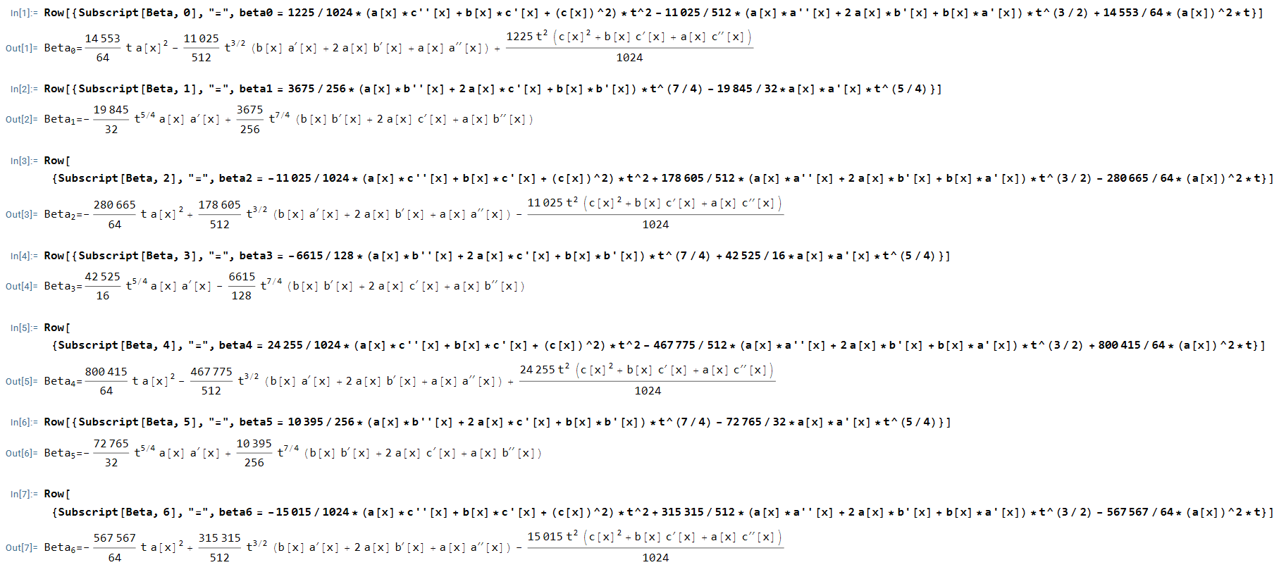
For brevity, we omit argument \(x\) below in functions \(a,b,c\) and their derivatives, i.e. we write \(a,a',a'',b,b',b'',c,c',c''\) instead of \(a(x),a'(x),a''(x),b(x),b'(x),b''(x),c(x),c'(x),c''(x)\). This omitting is justifiable because, first, only derivatives of function \(f\) are calculated symbolically, and second, \(x\) is constant when we expand \(f\) via Taylor’s formula (assuming \(t\to 0\)) and integrate in \(y\). However, we keep \(x\) in argument of function \(f\) and it is not possible to omit it. There will be some white spaces below because we wish our screenshots be of appropriate (readable) size and followed by the comments on the same page. First, we write \(\beta_0\), ..., \(\beta_6\), see Wolfram input and output below:

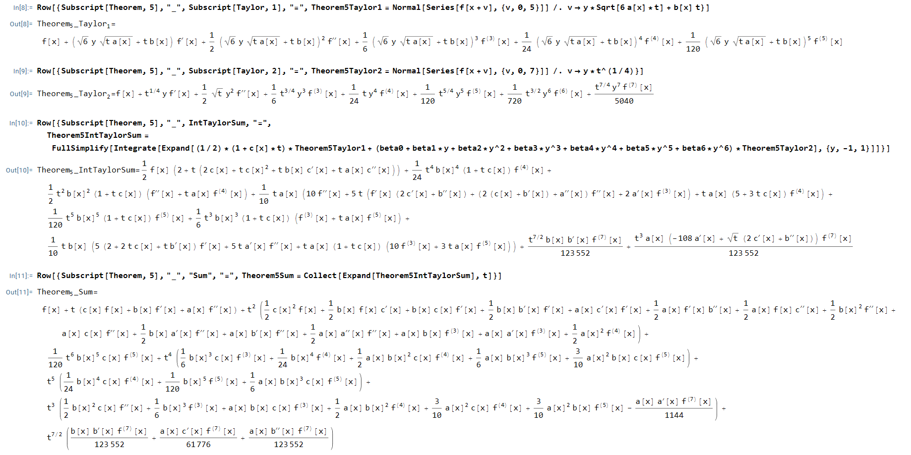
We use symbol \(Theorem_5\_Taylor_1\) to denote the Taylor expansion of the function
\(x\mapsto f(x+(6a(x)t)^{1/2}y+b(x)t)\) at the point \(x\) up to the 5th derivative, assuming that number \(y\in[-1,1]\) is fixed and \(t\to 0\), which gives us that \((6a(x)t)^{1/2}y+b(x)t\to0\). The residual terms with derivatives with powers greater than 5 we can represent in the Lagrange’s form for \(f \in C_b^6(\mathbb{R})\).

We use symbol \(Theorem_5\_Taylor_2\) to denote the Taylor expansion of the function \(x\mapsto f(x+yt^{1/4})\) at the point \(x\) up to the 7th derivative, assuming that number \(y\in[-1,1]\) is fixed and \(t\to 0\), which gives us that \(yt^{1/4})\). The residual terms with derivatives with powers greater than 7 we can represent in the Lagrange’s form for \(f \in C_b^8(\mathbb{R})\).

Then, we integrate \(\int\limits_{-1}^{1}\frac{1}{2}\Big(1+c(x)t\Big)Theorem_5\_Taylor_1dy+\int\limits_{-1}^{1}\Big(\beta_0(t,x)+\beta_1(t,x)y+\beta_2(t,x)y^2+\beta_3(t,x)y^3+\beta_4(t,x)y^4+\beta_5(t,x)y^5+\beta_6(t,x)y^6\Big)Theorem_5\_Taylor_2dy\) and denote this integral as \(Theorem_5\_IntTaylorSum\).

We group the terms of this expression into powers of \(t\) and denote \(Theorem_5\_Sum\)

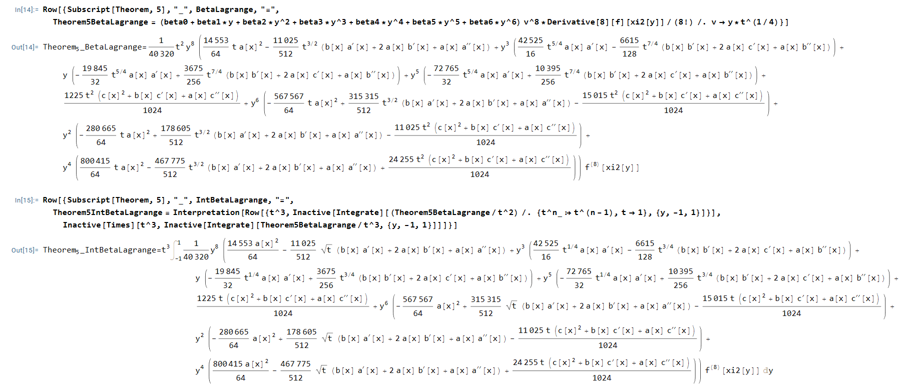
We also consider The Taylor expansion of the function \(f(x+(6a(x)t)^{1/2}y+b(x)t)\) at the point \(x\). We represent the remainder with the 6th derivative as a Lagrange’s form and denote it \(Teorem_5\_Lagrange\) Then we write the integral \(\int\limits_{-1}^{1}\frac{1}{2}\Big(1+c(x)t\Big)Theorem_5\_Lagrange dy\) We denote this integral \(Theorem_5\_IntLagrange\).

We also consider The Taylor expansion of the function \(f(x+yt^{1/4})\) at the point \(x\). We represent the remainder with the 8th derivative as a Lagrange’s form, multiply by \(\Big(\beta_0(t,x)+\beta_1(t,x)y+\beta_2(t,x)y^2+\beta_3(t,x)y^3+\beta_4(t,x)y^4+\beta_5(t,x)y^5+\beta_6(t,x)y^6\Big)\) and denote it \(Teorem_5\_BetaLagrange\) Then we write the integral \(\int\limits_{-1}^{1}\frac{1}{2}\Big(1+c(x)t\Big)Theorem_5\_Lagrange dy\) We denote this integral \(\int\limits_{-1}^{1}\frac{1}{2}\Big(1+c(x)t\Big)Theorem_5\_BetaLagrange dy\) We denote this integral

\(Theorem_5\_IntLagrange\).\(Theorem_5\_IntBetaLagrange\).

Then we sum \(Theorem_5\_Sum\), \(Theorem_5\_IntLagrange\) and \(Theorem_5\_IntBetaLagrange\). We get the final result.

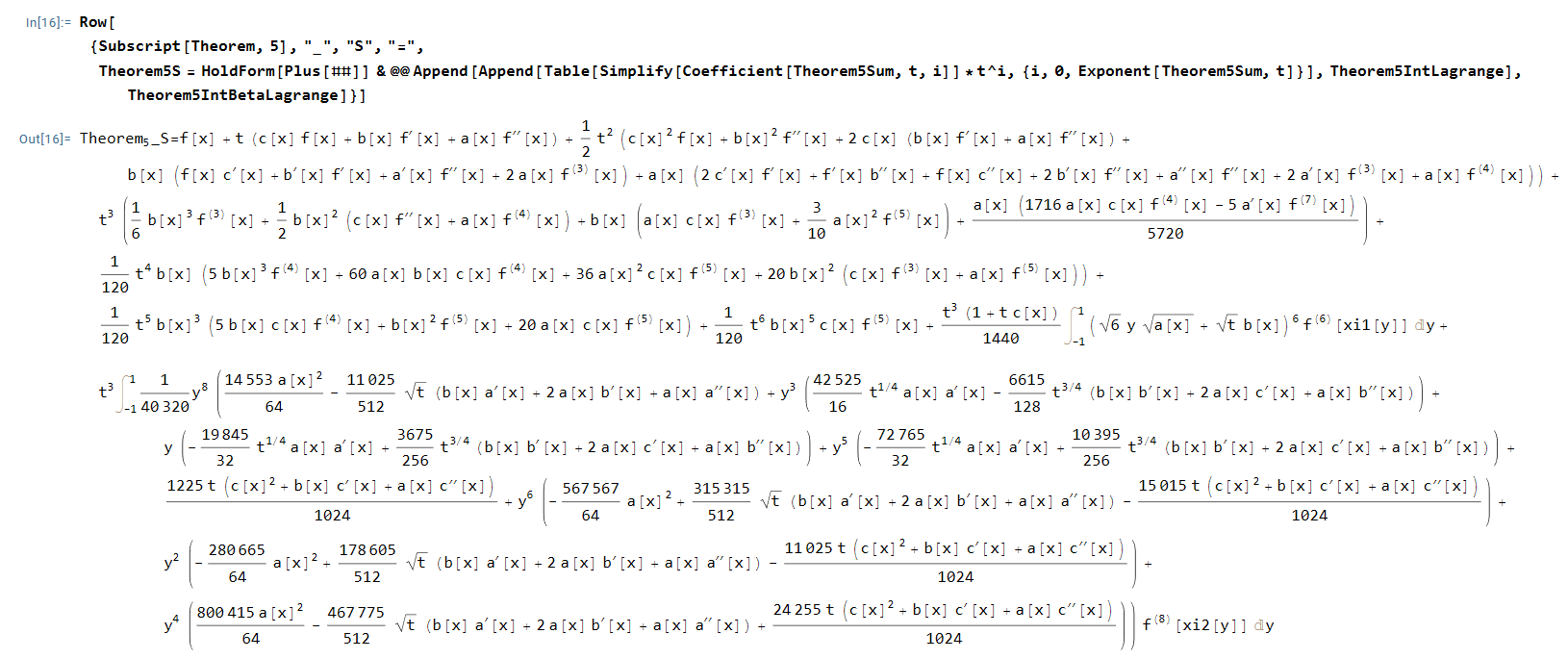
We have come to the following fact: the Chernoff function \(S(t)\), which is defined in (?? ) indeed satisfies item 3 of Theorem 5. This means that the coefficients in (?? ) are selected in such a way that \(S(t)f= f+tHf+\frac{1}{2}(tH)^2+o(t^2)\) as \(t \to +0\) for each \(f\in C_b^\infty(\mathbb{R})\).

References↩︎