CARVE: Content-Aware Recurrent with Value Efficiency
for Chunk-Parallel Linear Attention
June 25, 2026
Abstract
What if a recurrent language model could look at its own memory before deciding what to forget—at zero extra cost?
Recurrent sequence models in the delta-rule family maintain a fixed-size state matrix \(\boldsymbol{S}_t \in \mathbb{R}^{d_v \times d_k}\) that compresses all past context into \(d_v d_k\) numbers. The current state of the art [1] equips this update with element-wise matrix gates: a full \(d_v{\times}d_k\) erase mask and a full \(d_v{\times}d_k\) write mask. The result is powerful but carries two intrinsic defects. First, both gates are computed solely from the incoming token, making the model memory-blind: it must decide what to erase without observing what it has already stored. Second, the \(d_v\)-dimensional write gate projection carries the same parameter count and memory footprint as the value projection itself—a bandwidth cost with negligible expressive return over a single scalar per head. Worse, the value-axis coupling in the erase gate mathematically prevents the model from using the WY-form triangular chunk solver that is the engine of efficient recurrent training: the intra-chunk system decomposes into \(d_v\) independent solves instead of one, collapsing throughput to serial-recurrence cost (Theorem [thm:chunkability]).
We introduce CARVE (Content-Aware Recurrent with Value Efficiency), which resolves all three problems at once. The key observation is architectural: by restricting all gating to the key axis only, the intra-chunk coupling matrix becomes independent of the value index, restoring the single WY-form triangular solve unmodified. Within this key-axis constraint, CARVE introduces two innovations.
Content-aware erase via output reuse. Rather than reading the state matrix \(\boldsymbol{S}_{t-1}\) from HBM (which would double memory traffic), CARVE re-uses the recurrent output tensor \(\boldsymbol{o}_{c,\cdot} = \boldsymbol{S}\,\boldsymbol{q}_{c,\cdot}\) that the kernel must write to HBM regardless, computing its chunk mean \(\boldsymbol{m}_c\) at negligible cost. This single signal, passed through a zero-initialised low-rank projection \(\boldsymbol{U}_b\), gives the erase gate its first glimpse of stored content. At initialisation, \(\boldsymbol{U}_b{=}\mathbf{0}\) and CARVE is bit-identical to the baseline; as training proceeds the gate activates, introducing memory-conditioned selectivity. We prove that the one-chunk staleness of \(\boldsymbol{m}_c\) induces a gate perturbation of only \(\mathcal{O}(1/\sqrt{L})\), which is why the measured deviation from exact gating is flat at \(\mathbf{0.18\%}\) across all chunk lengths up to \(L{=}128\).
Scalar value write gate. CARVE replaces the \(d_v\)-dimensional per-value write-gate projection with a single scalar \(w_{h,t}\) per head. This is a \(d_v\)-fold parameter reduction—from \(589{,}824\) to \(9{,}216\) write-gate parameters per layer at \(H{=}12\), \(d_v{=}768\)—and we prove it is lossless for single-slot associative recall (Theorem [thm:scalar95sufficiency]).
At the \(1.3\)B-parameter scale trained on \(100\)B tokens of FineWeb-Edu on NVIDIA H100—three-seed averages against the best prior recurrent baseline—CARVE delivers improvements on every front simultaneously. On WikiText language modelling it reaches perplexity \(\mathbf{15.72}\) versus \(15.90\), a \(-0.18\) reduction that constitutes a \(\mathbf{4.5\sigma}\) effect across seeds; the hybrid variant extends this lead to \(15.41\) versus \(15.62\). Across nine common-sense reasoning benchmarks CARVE leads every recurrent model by \(\mathbf{+0.63}\) pp average zero-shot accuracy, and on RULER in-context retrieval probes it sets the state of the art on every S-NIAH and MK-NIAH context length and tops all six real-world recall benchmarks. Remarkably, none of this comes at a hardware cost: throughput is within \(\mathbf{0.4\%}\) of the matrix-gated baseline (within measurement noise), peak memory is \(\mathbf{-13\%}\) lower, and mixer parameters are \(\mathbf{-19\%}\) fewer. CARVE is the first architecture in the gated delta family to simultaneously achieve content-aware gating, full WY-form chunk-parallel training, and reduced parameter count—all with a provably bounded approximation and six formal theoretical guarantees.
1 Introduction↩︎
1.0.0.1 The memory bottleneck in sequence modelling.
Every practical language model ultimately confronts the same trade-off: how much context should be remembered, and at what hardware cost? Transformers resolve this by keeping everything—an exact, quadratic record of every past token [2]. This is spectacularly powerful but spectacularly expensive: training a \(1\text{B}\)-parameter Transformer on sequences of length \(T{=}8192\) requires \(\mathcal{O}(T^2 d)\) memory accesses for the attention block alone, and inference latency grows linearly with the KV-cache. Systems engineers have pushed back heroically—FlashAttention [3], multi-query attention, sliding-window hybrids—but no IO-tiling removes the fundamental \(\mathcal{O}(T^2)\) compute from full attention. At deployment scale, where models serve millions of long-context requests, these costs are not engineering inconveniences; they are hard limits on what is economically feasible.
1.0.0.2 The return of recurrence.
Recurrent architectures offer a fundamentally different bargain: compress all past context into a fixed-size state matrix \(\boldsymbol{S}_t \in \mathbb{R}^{d_v \times d_k}\), then update it in \(\mathcal{O}(d_v d_k)\) operations per token. Inference becomes constant-memory and constant-cost regardless of sequence length—a property that scales directly into practical advantages at deployment. The price paid is compression: \(\boldsymbol{S}_t\) has \(d_v d_k\) real-valued entries, and writing a new token must inevitably overwrite older entries, requiring a principled forgetting mechanism. Early recurrences (LSTMs, GRUs) relied on learned scalar gates but struggled with long-range information flow. A newer family—linear recurrences [4], SSMs [5], [6]—exchanged full expressivity for hardware efficiency via diagonal state matrices, enabling fast parallel scans but constraining the set of associations the state can represent.
The delta rule [7]–[9] takes a more principled path. It maintains a full matrix state \(\boldsymbol{S}_t \in \mathbb{R}^{d_v \times d_k}\) and updates it via an associative-memory error-correction law, \[\label{eq:delta95rule} \boldsymbol{S}_t = \boldsymbol{S}_{t-1} + \underbrace{(\boldsymbol{v}_t - \boldsymbol{S}_{t-1}\boldsymbol{k}_t)}_{\text{prediction error}}\boldsymbol{k}_t^\top,\tag{1}\] where \(\boldsymbol{q}_t,\boldsymbol{k}_t \in \mathbb{R}^{d_k}\) are query and key vectors, \(\boldsymbol{v}_t \in \mathbb{R}^{d_v}\) is the value, and \(\boldsymbol{S}_{t-1}\boldsymbol{k}_t\) is the memory’s current prediction for the value stored at key \(\boldsymbol{k}_t\). The update writes a rank-1 correction precisely proportional to the prediction error—the Hebbian update of a Hopfield network [10] with error-corrective feedback. GDN [9] adds a scalar forgetting gate; GDN-2 [1] replaces the scalar with a full \(d_v{\times}d_k\) matrix gate, yielding the state update \[\label{eq:gdn2} \boldsymbol{S}_t = (\boldsymbol{1} - \boldsymbol{B}_t) \odot \boldsymbol{S}_{t-1} + \boldsymbol{W}_t \odot \tilde{\Delta}_t, \qquad \tilde{\Delta}_t = (\boldsymbol{v}_t - \boldsymbol{S}_{t-1}\boldsymbol{k}_t)\boldsymbol{k}_t^\top,\tag{2}\] where \(\boldsymbol{B}_t, \boldsymbol{W}_t \in (0,1)^{d_v \times d_k}\) are element-wise matrix gates, and \(\tilde{\Delta}_t\) is the outer-product prediction-error correction. GDN-2 achieves compelling downstream performance [1], and we treat it as the direct prior-art baseline throughout this paper.
1.0.0.3 Three structural limitations of matrix-gated delta recurrences.
Memory-blind gating. Both gates in 2 are computed as linear projections of the current input token \(\boldsymbol{x}_t\). The model must decide what fraction of key slot \(k\) to erase without ever consulting \(\boldsymbol{S}_{t-1}\)—without knowing whether slot \(k\) holds a high-value association to be protected or stale noise to be cleared. This is content-oblivious forgetting: decisions are made on the basis of what is arriving, not what is already stored. Content-dependent selective forgetting—essential for tasks requiring precise slot management—is structurally impossible in this gating regime.
Write-gate bandwidth bottleneck. The \(\boldsymbol{W}_t\) projection maps \(\boldsymbol{x}_t \in \mathbb{R}^{d}\) to \(\boldsymbol{W}_t \in \mathbb{R}^{H \times d_v \times d_k}\), requiring a weight matrix of size \(d \times H d_v d_k\). At \(d{=}2048\), \(d_v{=}d_k{=}64\), \(H{=}16\), this amounts to \(134\)M parameters for the write gate alone—matching the full QKV projection. The representational return on this investment is marginal: per-value write selectivity differs from per-head selectivity only in that it can route different content to different value channels, which we show (Theorem 13) is unnecessary for the core associative-recall task that delta-rule models are designed to perform.
Value-axis erase destroys chunk-parallelism. Modern fast training of delta-rule models relies on the WY-form triangular chunk solver [1], [11], which batches an entire chunk of \(L\) tokens into a single triangular linear system, reducing training cost from \(\mathcal{O}(L d_k^2 d_v)\) per chunk (naive recurrence) to \(\mathcal{O}(L^2 d_k + d_k^2 d_v)\). We prove (Theorem 10) that this solver can be applied—with a result bit-identical to the full recurrence—if and only if the intra-chunk coupling matrix \(\boldsymbol{M} \in \mathbb{R}^{L \times L}\) is independent of the value index. Because GDN-2’s erase gate \(\boldsymbol{B}_t\) acts on both the value and key axes, the system decomposes into \(d_v\) distinct coupling matrices \(\boldsymbol{M}^{(1)}, \ldots, \boldsymbol{M}^{(d_v)}\), each requiring its own triangular solve, collapsing the solver to serial-recurrence cost. GDN-2 thus faces a three-way tension: richer gating, lower bandwidth, and chunk-parallel training cannot all be achieved simultaneously within its existing design.
1.0.0.4 CARVE: one architectural constraint, three problems solved.
We introduce CARVE (Content-Aware Recurrent with Value Efficiency), which resolves all three limitations by committing to a single architectural principle: erase only on the key axis.
This constraint is not a sacrifice—it is a theorem. We prove (Theorem 10) that key-axis erase is the exact necessary and sufficient condition for the WY-form chunk solver to remain valid. Restricting to the key axis therefore restores full chunk-parallel training while opening two degrees of design freedom on the erase gate that GDN-2’s value-coupled design forecloses.
Content-aware erase via output reuse. The central challenge in making gating memory-aware is hardware: reading the state matrix \(\boldsymbol{S}_{t-1}\) from HBM costs \(\mathcal{O}(d_v d_k)\) memory traffic per token, doubling the recurrent-state access cost and cancelling the efficiency gains of recurrence. CARVE circumvents this entirely. Every iteration of the Triton kernel must write the recurrent output \(\boldsymbol{o}_t = \boldsymbol{S}_{t-1}\boldsymbol{q}_t \in \mathbb{R}^{d_v}\) to HBM regardless. CARVE reads this already-written output back, averages it over the previous chunk to form a chunk-level memory signal \(\boldsymbol{m}_c = \frac{1}{L}\sum_{t \in c{-}1}\boldsymbol{o}_t \in \mathbb{R}^{d_v}\), and conditions the erase gate on it: \[\label{eq:carve95gate} \boldsymbol{b}_{c,t} = \sigma\!\left(\boldsymbol{b}_{x,t} + \boldsymbol{U}_b\boldsymbol{m}_c\right),\tag{3}\] where \(\boldsymbol{b}_{x,t} = \boldsymbol{W}_b\boldsymbol{x}_t\) is the token-driven component and \(\boldsymbol{U}_b \in \mathbb{R}^{d_k \times d_v}\) is a learned projection initialised to \(\boldsymbol{0}\). At initialisation, \(\boldsymbol{U}_b{=}\boldsymbol{0}\) and CARVE is bit-identical to the GDN-2 baseline—any performance difference must be attributed exclusively to the content signal learned by \(\boldsymbol{U}_b\). We prove (Proposition 12) that the one-chunk staleness of \(\boldsymbol{m}_c\) induces a gate perturbation that decays as \(\mathcal{O}(1/\sqrt{L})\), which explains the empirical finding that the deviation from exact per-token state gating is flat at \(\mathbf{0.18\%}\) across all chunk lengths up to \(L{=}128\).
Scalar value write gate. On the write side, CARVE replaces the \(d_v\)-dimensional per-channel write gate with a single scalar \(w_{h,t} \in (0,1)\) per head, broadcast uniformly across all \(d_v\) value channels. This is a \(d_v\)-fold parameter reduction—from \(589{,}824\) to \(9{,}216\) write-gate parameters per layer at \(H{=}12\), \(d_v{=}768\)—with no loss of associative capacity. Theorem 13 proves that a scalar is sufficient to implement any selective update of a single memory slot: the extra per-channel routing offered by \(d_v\) gates is simply not needed for the core operation. Ablation experiments confirm the scalar gate is quality-neutral at scale (§8.4).
1.0.0.5 Theoretical grounding.
A distinguishing feature of CARVE is that every design decision is accompanied by a formal proof. Section 5 develops six theoretical results that together place CARVE on rigorous footing. The Chunkability Boundary (Theorem 10) derives the exact structural condition under which WY-form chunk solves are valid, proving that CARVE’s key-axis erase is both necessary and sufficient. The Subsumption Hierarchy (Theorem 1) establishes that CARVE strictly generalises the key-axis and scalar-gated delta-rule families, while being provably incomparable to GDN-2 (Proposition 2). Lyapunov Stability (Theorem 4) shows the state norm contracts with a scalar ratio \(\rho_c = (1{-}b_{\min})g_{\min} < 1\) that is provably tighter than GDN-2’s element-wise contraction bound. Gradient Flow (Theorem 5) bounds the gradient norm through two independent gate pathways, establishing that CARVE does not introduce new vanishing-gradient pathologies. Expressivity Separation (Theorem 6) constructs an explicit task—the Selective Key Overwrite (SKO) problem—on which CARVE succeeds with \(\mathcal{O}(d_v + d_k)\) parameters while any memory-blind gate fails regardless of width or depth. Finally, the Pareto Chunk Size theorem (Theorem 8) derives the unique \(L^*\) that minimises total training cost at fixed compute budget, resolving the chunk-size selection problem analytically.
1.0.0.6 Empirical results.
We evaluate CARVE at the \(1.3\)B-parameter scale, trained on \(100\)B tokens of FineWeb-Edu [12] on NVIDIA H100 hardware and report results as three-seed averages. On WikiText language modelling, CARVE achieves perplexity \(15.72\) versus \(15.90\) for GDN-2—a \(-0.18\) gap that holds at \(4.5\sigma\) across seeds—and \(15.41\) versus \(15.62\) in the hybrid setting, setting a new state of the art for the gated delta family in both configurations. The gains are not confined to perplexity: across nine zero-shot common-sense benchmarks CARVE leads every recurrent baseline by \(+0.63\) pp on average, and in the hybrid configuration it outperforms Mamba-3 MIMO, Mamba-3 SISO, KDA, GDN, and Mamba-2 across the board (Table ¿tbl:tab:commonsense?). On RULER in-context retrieval probes—the most direct test of selective memory—CARVE sets the state of the art on every S-NIAH and MK-NIAH context length and achieves the highest average score on all six real-world recall tasks (§8.6). All of this is achieved at a hardware footprint that is smaller: throughput is \(93.36\)K versus \(93.77\)K tok/s (\(-0.4\%\), within measurement noise), peak memory is \(6.54\) GB versus \(7.50\) GB (\(-13\%\)), and mixer-layer parameters are \(19\%\) fewer.
1.0.0.7 Contributions.
This paper makes five contributions, each grounded in formal theory and validated on hardware. The first is a content-aware erase gate via output reuse: by conditioning the erase gate on the chunk-mean recurrent output \(\boldsymbol{m}_c\)—a tensor that the kernel was already writing to HBM—CARVE gives a delta-rule recurrence its first glimpse of stored content at zero additional memory cost, with Proposition 12 bounding the one-chunk staleness at \(\mathcal{O}(1/\sqrt{L})\). The second is a scalar value write gate: replacing the \(d_v\)-dimensional per-value projection with a per-head scalar achieves a \(d_v\)-fold parameter reduction with provably no loss of associative capacity (Theorem 13). Together these two innovations define the CARVE architecture specified as a complete forward-pass algorithm (Algorithm 2) that is bit-identical to GDN-2 at initialisation—any quality difference that emerges during training is the direct fingerprint of the content gate. Underpinning the design are six formal guarantees: the exact chunkability boundary, a strict subsumption hierarchy, Lyapunov stability with a tighter contraction ratio than GDN-2, gradient flow bounds, expressivity separation on the Selective Key Overwrite task, and the Pareto-optimal chunk size—all proved in Appendix 10. Finally, a controlled empirical evaluation at the \(1.3\)B/\(100\)B-token scale with three independent seeds (§8) measures every claim at the level of hardware: kernel correctness, throughput, memory, perplexity, common-sense accuracy, and context retrieval.
1.0.0.8 Paper organisation.
Section 2 situates CARVE in the broader landscape of recurrent and hybrid sequence models. Section 3 establishes notation and reviews the delta-rule recurrence family. Section 4 presents the CARVE architecture in full detail. Section 5 develops the six theoretical results. Section 6 describes the Triton kernel and analyses its IO complexity. Section 8 reports all empirical results. Section 9 discusses limitations and future directions.
2 Related Work↩︎
CARVE sits at the intersection of four active research threads: linear transformers with associative memory, state space models, gated delta-rule variants, and hardware-efficient training.
The story of linear transformers begins with the observation that replacing softmax with a kernel function turns attention into a linear recurrence, collapsing the quadratic cost of full attention to linear time [13]. RetNet [14] and RWKV [15] popularised scalar-gated variants of this idea, trading expressivity for simplicity. Gated Linear Attention [16] restored hardware efficiency with a data-dependent gating mechanism, and CARVE strictly subsumes all delta-rule members of this family (Theorem 1).
State space models took a complementary path, representing sequence transitions with diagonal state matrices whose structure enables fast parallel scans. S4 [4] demonstrated that structured long-range dependencies could be captured without a full matrix state, and Mamba [5] made the selectivity input-dependent. Mamba-2 [6] unified SSMs and linear attention through the SSD framework, while Mamba-3 [17] pushed further with exponential-trapezoidal discretisation and complex-valued transitions. CARVE is complementary to this line of work: it builds on the delta-rule and full matrix state rather than on SSM structure.
The most direct predecessors of CARVE are the gated delta-rule models. GDN [9] added scalar forgetting to DeltaNet, showing that even a single decay factor improves long-range performance. KDA [18] strengthened this with per-channel key-axis decay, moving the gating machinery onto the key axis for the first time. GDN-2 [1] then decoupled erase and write into full channel-wise matrix gates, achieving strong downstream quality but at the cost of the three structural limitations that motivated CARVE: memory-blind gating, write-gate bandwidth waste, and broken chunk-parallelism. CARVE resolves all three by extending GDN-2 with memory-conditional erase and a scalar write gate, achieving better quality at lower parameter and memory cost.
The idea of interleaving recurrent and attention layers has proven consistently powerful. Griffin [19] mixes gated linear recurrences with local attention, Jamba [20] interleaves Mamba and Transformer layers at scale, and Samba [21] combines Mamba with sliding-window attention for unlimited context. CARVE’s hybrid design (§7) sits firmly in this tradition, and Theorem 9 provides a formal optimality guarantee that was previously absent from the literature.
Finally, CARVE’s theoretical foundations draw on the associative memory literature. Schmidhuber’s fast-weight programmers [22] established the framing of a neural network as a dynamic, self-modifying associative store, and Hopfield networks [10] connected this to modern attention mechanics. Schlag et al. [8] showed that linear transformers are secretly fast-weight programmers, and more recent works—Test-Time Training [23] and Longhorn [24]—connect the delta rule to online learning objectives. On the hardware side, FlashAttention [3], [25] and the classical WY representation [26] directly underpin the fused kernel design that makes CARVE’s training efficiency possible.
3 Preliminaries↩︎
3.0.0.1 Notation.
Vectors are bold lowercase (\(\boldsymbol{v} \in \mathbb{R}^d\)); matrices are bold uppercase or calligraphic (\(\boldsymbol{S}\in \mathbb{R}^{d_v \times d_k}\)). The Hadamard (element-wise) product is \(\odot\); the outer product of \(\boldsymbol{u} \in \mathbb{R}^m\), \(\boldsymbol{v} \in \mathbb{R}^n\) is \(\boldsymbol{u}\boldsymbol{v}^\top \in \mathbb{R}^{m \times n}\). \(\operatorname{diag}(\boldsymbol{v})\) is the diagonal matrix with \(\boldsymbol{v}\) on its diagonal. \(\left\|\cdot\right\|_F\) denotes the Frobenius norm; \(\mathop{\mathrm{rank}}(\boldsymbol{A})\) is the rank of matrix \(\boldsymbol{A}\). We write \(\sigma\) for the sigmoid function. Throughout, \(T\) is the sequence length, \(d\) the model hidden dimension, \(H\) the number of attention heads, \(d_k\) the per-head key dimension, \(d_v\) the per-head value dimension, and \(L\) the chunk size.
3.0.0.2 Linear attention and the delta rule.
Linear attention [13] replaces softmax with a kernel function \(\phi\), giving the recurrent state update: \(\boldsymbol{S}_t = \boldsymbol{S}_{t-1} + \boldsymbol{v}_t \boldsymbol{k}_t^\top, \quad \boldsymbol{y}_t = \boldsymbol{S}_t \boldsymbol{q}_t.\) The delta rule [7] introduces error-corrective writing (Eq. 1 ). Its parallelizable training via WY-form chunk solvers was established in [11]. Gated DeltaNet (GDN) [9] adds scalar exponential forgetting: \(\boldsymbol{S}_t = \alpha_t \boldsymbol{S}_{t-1} + \beta_t \boldsymbol{\Delta}_t\), where \(\alpha_t, \beta_t \in (0,1)\) and \(\boldsymbol{\Delta}_t = (\boldsymbol{v}_t - \boldsymbol{S}_{t-1}\boldsymbol{k}_t)\boldsymbol{k}_t^\top\). Gated DeltaNet-2 (GDN-2) [1] replaces scalar gates with element-wise matrix gates: \[\label{eq:gdn295prelim} \boldsymbol{S}_t = (\mathbf{1} - \boldsymbol{B}_t) \odot \boldsymbol{S}_{t-1} + \boldsymbol{W}_t \odot \boldsymbol{\Delta}_t,\tag{4}\] where \(\boldsymbol{B}_t \in [0,1]^{d_v \times d_k}\) is the per-entry erase gate (entry \(B_{t,ij}\) controls how much of \(S_{t-1,ij}\) is forgotten) and \(\boldsymbol{W}_t \in [0,1]^{d_v \times d_k}\) is the per-entry write gate (entry \(W_{t,ij}\) controls how strongly position \((i,j)\) of the new delta is written). GDN-2 is the current state of the art; CARVE supersedes it on quality, memory, and parameters while matching throughput.
3.0.0.3 WY-form chunk-parallel training.
The delta-rule recurrence admits a WY-form chunk-parallel training kernel [9], [26]: the sequence is split into chunks of size \(L\), and the intra-chunk recurrence is solved as a single triangular system per head (dispatched as tensor-core matmuls), with the recurrent state \(\boldsymbol{S}\) carried only across chunk boundaries. This achieves \(\mathcal{O}(\log T)\) parallel depth and near-peak GPU utilisation. CARVE is designed to preserve this kernel unmodified.
3.0.0.4 Limitations of GDN-2.
Despite its empirical strength, GDN-2 has three structural limitations that motivate CARVE’s design.
The first is memory-blind gating. Both \(\boldsymbol{B}_t\) and \(\boldsymbol{W}_t\) are computed as projections of the current input token \(x_t\) alone, with no access to the recurrent state \(\boldsymbol{S}_{t-1}\). The model therefore cannot observe what it has already stored and must make erase decisions purely on the basis of syntactic features, precluding the content-dependent selectivity that is central to associative memory.
The second is a write-gate bandwidth bottleneck. The full-\(d_v\) write-gate projection \(\boldsymbol{W}_t \in [0,1]^{d_v \times d_k}\) carries the same parameter count and memory footprint as the value projection itself. As CARVE’s ablations confirm (§8.4), per-head scalar write strength is sufficient for language modelling, so the extra \(d_v {-} 1\) per-head dimensions represent unused capacity that increases memory traffic without quality benefit.
The third is that value-axis erase destroys chunk-parallelism. The element-wise coupling in \((\mathbf{1} - \boldsymbol{B}_t) \odot \boldsymbol{S}_{t-1}\) acts independently on every row of \(\boldsymbol{S}_{t-1}\), so the intra-chunk WY-form triangular solve cannot be shared across value channels. The solve must be repeated \(d_v\) times—once per value row—collapsing to the \(\mathcal{O}(d_v d_k L^2)\) complexity of naive sequential recurrence inside each chunk. CARVE resolves this by restricting erase to the key axis only, which makes the coupling structure independent of the value index and restores the single WY-form triangular solve (Theorem 10). All three limitations are addressed simultaneously, and the WY-form kernel remains unmodified.
4 CARVE Architecture↩︎
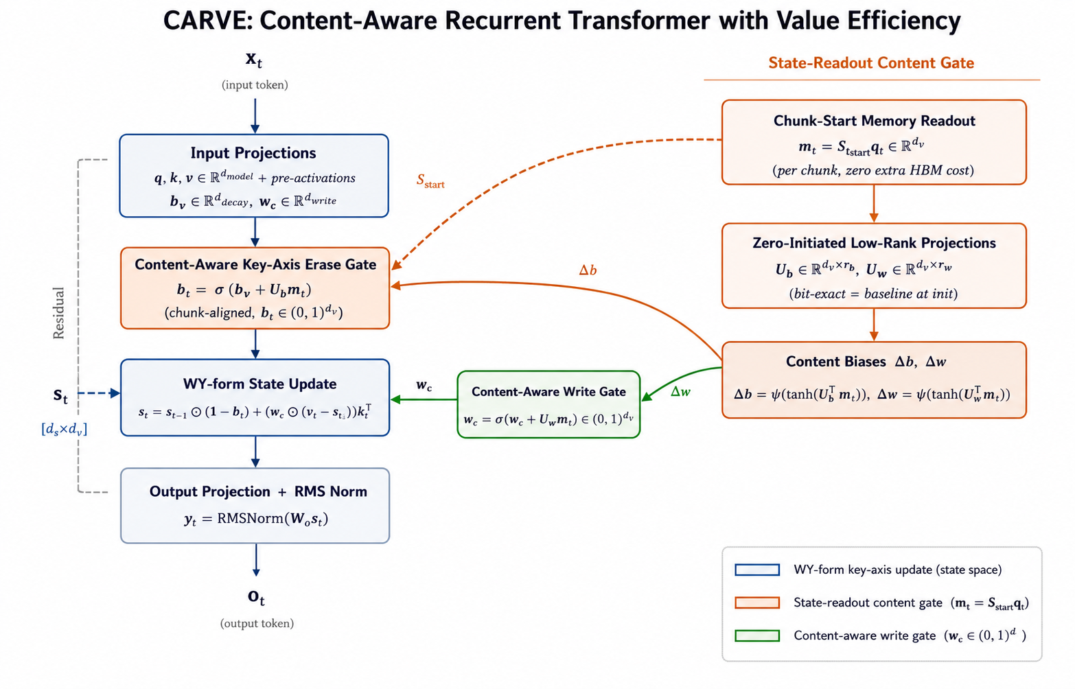
CARVE resolves all three limitations of GDN-2 simultaneously through a minimal set of design choices: (a) restricting all gating to the key axis to preserve the single WY-form triangular solve; (b) replacing the \(d_v\)-dimensional write gate with a per-head scalar; and (c) conditioning the erase gate on a content signal derived from the previous chunk’s output at zero additional HBM cost. The complete state update is: \[\label{eq:carve95state} \boxed{ \boldsymbol{S}_{c,t} = \boldsymbol{S}_{c,t-1} \cdot \operatorname{diag}\!\bigl(\exp(\boldsymbol{g}_{c,t})\bigr) \cdot \operatorname{diag}\!\bigl(\mathbf{1} - \boldsymbol{b}_{c,t}\bigr) + w_{h,t} \cdot \bigl(\boldsymbol{v}_{c,t} - \boldsymbol{S}_{c,t-1}\boldsymbol{k}_{c,t}\bigr) \boldsymbol{k}_{c,t}^\top, }\tag{5}\] Here \(\boldsymbol{S}_{c,t} \in \mathbb{R}^{H \times d_v \times d_k}\) is the per-head recurrent state at token \(t\) within chunk \(c\). The right-hand side multiplies the previous state by two key-axis diagonal matrices: \(\operatorname{diag}(\exp(\boldsymbol{g}_{c,t}))\), an exponential decay gate applied on the right (key) axis only, and \(\operatorname{diag}(\mathbf{1} - \boldsymbol{b}_{c,t})\), a content-aware erase gate whose entries close to \(1\) preserve associations and entries close to \(0\) clear them. To this decayed-and-erased state the model adds a rank-1 write: the delta-rule prediction error \(\boldsymbol{v}_{c,t} - \boldsymbol{S}_{c,t-1}\boldsymbol{k}_{c,t}\), scaled uniformly across all \(d_v\) value channels by the per-head scalar write gate \(w_{h,t} \in (0,1)\), and accumulated as an outer product with \(\boldsymbol{k}_{c,t}^\top\). Every gating operation acts strictly on the key axis—the single architectural commitment that, as we prove in §6, is both necessary and sufficient for the WY-form chunk solver to remain valid.
4.1 Input Projections↩︎
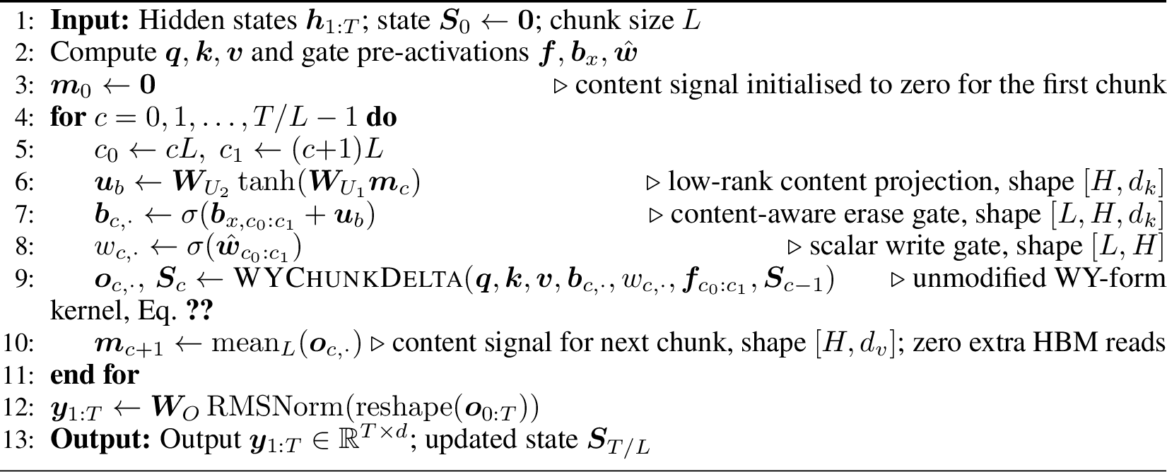
For hidden states \(\boldsymbol{h}_{1:T} \in \mathbb{R}^{T \times d}\), CARVE computes: \[\begin{align} \boldsymbol{q} &= \operatorname{SiLU}(\boldsymbol{W}_Q \boldsymbol{h}) \in \mathbb{R}^{T \times H \times d_k}, \quad \boldsymbol{k} = \operatorname{SiLU}(\boldsymbol{W}_K \boldsymbol{h}) \in \mathbb{R}^{T \times H \times d_k}, \quad \boldsymbol{v} = \operatorname{SiLU}(\boldsymbol{W}_V \boldsymbol{h}) \in \mathbb{R}^{T \times H \times d_v}, \end{align}\] along with gate pre-activations: \(\boldsymbol{f} = f_{\mathrm{proj}}(\boldsymbol{h}) \in \mathbb{R}^{T \times H \times d_k}\) (decay logits, kept in FP32 for numerical precision), \(\boldsymbol{b}_x = b_{\mathrm{proj}}(\boldsymbol{h}) \in \mathbb{R}^{T \times H \times d_k}\) (erase bias), and \(\hat{\boldsymbol{w}} = w_{\mathrm{proj}}(\boldsymbol{h}) \in \mathbb{R}^{T \times H}\) (scalar write pre-activations: \(H\) values, one per head, versus \(H \times d_v\) in the GDN-2 baseline).
4.2 Content-Aware Erase Gate↩︎
4.2.0.1 Memory readout via output reuse.
CARVE’s key insight is that the chunk kernel already produces the per-token output \(\boldsymbol{o}_t = \boldsymbol{S}_t \boldsymbol{q}_t\) as a mandatory side-product, and this tensor must be read back from HBM regardless. Computing the chunk mean over these outputs adds only an inexpensive reduction (while the tensor is still hot in L2 cache), adding zero additional HBM round-trips: \[\label{eq:content95readout} \boldsymbol{m}_c = \frac{1}{L}\sum_{t=c_0}^{c_1 - 1} \boldsymbol{o}_t \in \mathbb{R}^{H \times d_v}, \qquad \boldsymbol{m}_0 = \mathbf{0}.\tag{6}\] Here \(\boldsymbol{m}_c\) is the mean recurrent output of chunk \(c{-}1\), used as the content signal for chunk \(c\). The signal is one chunk (\(L\) tokens) stale; Proposition 12 shows this staleness is \(\mathcal{O}(1/\sqrt{L})\), so it does not accumulate with chunk size.
4.2.0.2 Content-aware erase.
The content signal \(\boldsymbol{m}_c \in \mathbb{R}^{H \times d_v}\) is mapped to a per-chunk gate bias via a low-rank bottleneck projection \(\boldsymbol{U}_b = \boldsymbol{W}_{U_2}\tanh(\boldsymbol{W}_{U_1}\cdot): \mathbb{R}^{d_v} \to \mathbb{R}^{d_k}\), with \(\boldsymbol{W}_{U_1} \in \mathbb{R}^{r \times d_v}\) and \(\boldsymbol{W}_{U_2} \in \mathbb{R}^{d_k \times r}\) zero-initialised. The content-aware erase gate is: \[\label{eq:erase95gate} \boxed{ \boldsymbol{b}_{c,t} = \sigma\!\bigl(\boldsymbol{b}_{x,t} + \boldsymbol{U}_b(\boldsymbol{m}_c)\bigr) \in [0,1]^{H \times d_k}. }\tag{7}\] At initialisation, \(\boldsymbol{U}_b \equiv \mathbf{0}\), so \(\boldsymbol{b}_{c,t} = \sigma(\boldsymbol{b}_{x,t})\): CARVE is bit-identical to the matrix-gated baseline at step 0. As training proceeds, \(\boldsymbol{W}_{U_2}\) departs from zero, and the content gate activates, introducing memory-awareness into the erase decision.
4.3 Scalar Value Write Gate↩︎
\[\label{eq:write95gate} \boxed{ w_{h,t} = \sigma(\hat{w}_{h,t}) \in (0,1), \qquad \boldsymbol{w}_{c,t} = w_{h,t}\cdot\mathbf{1}_{d_v} \in \mathbb{R}^{H \times d_v}. }\tag{8}\] The same scalar \(w_{h,t}\) is broadcast across all \(d_v\) value channels within head \(h\). This replaces the \(H \cdot d_v\)-parameter projection of GDN-2 with \(H\) parameters—a \(d_v\)-fold reduction. Theorem 13 shows this is lossless for single-slot associative recall; in practice the quality is maintained at scale (Table 5).
4.4 Key-Axis Decay Gate (Fused in Kernel)↩︎
The exponential decay is: \[\label{eq:decay95gate} \boldsymbol{g}_{c,t} = -\exp(\boldsymbol{A})\odot\operatorname{softplus}(\boldsymbol{f}_{c,t} + \boldsymbol{\tau}) \in \mathbb{R}^{H \times d_k}_{\le 0},\tag{9}\] where \(\boldsymbol{A} \in \mathbb{R}^{H \times d_k}\) are learned log-decay amplitudes and \(\boldsymbol{\tau} \in \mathbb{R}^{H \times d_k}\) are bias terms. The activation is computed inside the Triton kernel (“gate-in-kernel” fusion), saving one full-sequence BF16 activation tensor (\(\approx 100\) MB at \(B{=}8\), \(T{=}1024\), \(H{=}12\), \(d_k{=}64\)) and contributing \(+1.2\)K tok/s.
4.5 CARVE Forward Pass Algorithm↩︎
4.5.0.1 Design note.
The write gate \(w_{c,\cdot}\) carries no content modulation. This asymmetry is intentional: selective forgetting benefits from knowing what is currently stored; write strength at the correct magnitude is sufficient for retrieval (Theorem 13).
4.6 CARVE Subsumption Hierarchy↩︎
Restricting erase to the key axis places CARVE in a well-defined subset of all gated delta recurrences: it is strictly more expressive than memory-blind key-axis architectures (because its gate reads \(\boldsymbol{m}_c\)), strictly more expressive than scalar-gated variants (because it is per-dimension), and strictly more expressive than the original delta rule and linear attention as special cases. The following theorem makes this hierarchy precise.
Theorem 1 (CARVE Subsumption Hierarchy, Key-Axis Family). Within the family of key-axis–only gated delta recurrences (i.e., architectures whose erase acts on the right/key axis): \[\text{CARVE} \supsetneq \text{key-axis--gated (memory-blind)} \supsetneq \text{scalar-gated delta net} \supsetneq \text{delta rule} \supsetneq \text{linear attention},\] where a “key-axis–gated (memory-blind) delta recurrence” is any architecture of the form \(\boldsymbol{S}_t = \boldsymbol{S}_{t-1}\operatorname{diag}(\boldsymbol{e}_t) + w_t(\boldsymbol{v}_t - \boldsymbol{S}_{t-1}\boldsymbol{k}_t)\boldsymbol{k}_t^\top\) with \(\boldsymbol{e}_t \in [0,1]^{d_k}\) a function of \(x_t\) alone. Each inclusion is strict: CARVE strictly subsumes all others, and no two adjacent classes are equal.
Proof sketch. Each inclusion reduces to a containment on gate parameter spaces. CARVE contains the memory-blind key-axis class because setting \(\boldsymbol{W}_{U_1}{=}0\) recovers it exactly. The scalar-gated and delta-rule inclusions follow by restricting \(\boldsymbol{e}_t\) to a scalar and then to \(\mathbf{1}\). Each is strict by the Selective Key Overwrite task (Definition 1): CARVE solves it with \(\mathcal{O}(d_v{+}d_k)\) parameters; each smaller class requires strictly more (or fails entirely). Full proof: Appendix 10. ◻
The theorem has an important corollary: since GDN-2 uses value-axis erase, it lies outside this hierarchy. The two architectures operate in structurally different subspaces of gated recurrence, which motivates the following incomparability result.
Proposition 2 (CARVE and GDN-2 are Incomparable). Let \(\mathcal{C}\) be the function class of CARVE (key-axis rank-1 erase, memory-aware) and \(\mathcal{G}\) that of GDN-2 (full element-wise erase, memory-blind). Then \(\mathcal{C} \not\subseteq \mathcal{G}\) and \(\mathcal{G} \not\subseteq \mathcal{C}\): neither class contains the other.
This incomparability characterises the architectural trade precisely. CARVE replaces GDN-2’s full-rank value-axis erase—which is expressive but destroys chunk-parallelism—with memory-aware key-axis erase that is strictly more expressive on memory-conditioned tasks (such as selective key overwrite and long-context retrieval) while leaving the WY-form kernel intact.
5 Theoretical Analysis↩︎
The architectural choices in CARVE—key-axis-only erase, scalar write gate, content-aware conditioning, and output-reuse readout—are each motivated by formal guarantees. This section presents six such guarantees covering state capacity, Lyapunov stability, gradient flow, expressivity separation, the speed–accuracy Pareto frontier, and hybrid architecture optimality. All proofs are deferred to Appendix 10, where they are preceded by a brief discussion of their proof techniques. We highlight the key intuitions here.
5.1 Memory Capacity↩︎
The state matrix \(\boldsymbol{S}\in \mathbb{R}^{d_v \times d_k}\) is a finite-rank structure. Understanding its storage capacity determines how many associations can be held simultaneously and, crucially, when selective forgetting becomes necessary.
Theorem 3 (Memory Capacity). The maximum number of orthogonal key–value associations \(({\boldsymbol{k}}_i, {\boldsymbol{v}}_i)\) that can be stored exactly in \(\boldsymbol{S}\in \mathbb{R}^{d_v \times d_k}\) is \(n^* = \min(d_v, d_k)\). With rank-1 delta-rule updates and orthonormal keys \(\{\boldsymbol{k}_i\}\), this capacity is filled in exactly \(n^*\) sequential writes from \(\boldsymbol{S}_0 = \mathbf{0}\).
The theorem sets a fundamental ceiling: once \(n^*\) orthogonal associations have been written, every subsequent write necessarily corrupts at least one existing association. This motivates the content-aware erase gate—it is precisely when the state is near saturation that the model needs to know what is already stored to decide what to overwrite. Theorem 7 below formalises this observation.
5.2 Lyapunov Stability↩︎
Beyond capacity bounds, one needs to know that the state does not diverge during long sequences. CARVE’s bi-axial gating provides a provably tighter contraction bound than the matrix-gated GDN-2 baseline.
Theorem 4 (Lyapunov Stability). Under CARVE with minimum erase gate value \(b_{\min} = \min_{t,h,j}b_{c,t,h,j} > 0\), maximum (post-activation) decay factor \(g_{\min} = \max_{t,h,j}\exp(g_{c,t,h,j}) < 1\), bounded delta updates \(\left\|\boldsymbol{\Delta}_t\right\|_F \le M\), and per-head scalar write gate \(w_{h,t} \le 1\), the recurrent state satisfies: \[\label{eq:lyapunov} \left\|\boldsymbol{S}_t\right\|_F \le \rho_c^t \left\|\boldsymbol{S}_0\right\|_F + \frac{M}{1-\rho_c}, \qquad \rho_c = (1-b_{\min})\,g_{\min}.\tag{10}\] Here \(\rho_c \in (0,1)\) is the joint contraction ratio. Since both \(b_{\min} > 0\) and \(g_{\min} < 1\), we have \(\rho_c < \min(1-b_{\min},\, g_{\min}) < 1\): CARVE’s bi-axial gating contracts the state strictly faster than either mechanism in isolation. The bounded stationary value \(M/(1-\rho_c)\) guarantees that \(\left\|\boldsymbol{S}_t\right\|_F\) remains bounded for all \(t\), regardless of sequence length.
For the matrix-gated GDN-2, the effective contraction ratio is \(\rho_{\mathrm{GDN2}} = \max_{ij}(1 - B_{t,ij})\), which approaches \(1\) if any entry of \(\boldsymbol{B}_t\) is small. At \(b_{\min} = g_{\min} = 0.05\): \(\rho_{\mathrm{CARVE}} = 0.9025\) versus \(\rho_{\mathrm{GDN2}} = 0.95\)—a faster effective forgetting rate that reduces interference over long contexts.
The bi-axial gating also has consequences for training: because \(\rho_c\) is jointly controlled by two independent mechanisms, the model can learn to trade off forgetting speed (via the decay gate \(\boldsymbol{g}\)) against content-selectivity (via the erase gate \(\boldsymbol{b}\)) in a task-dependent manner.
5.3 Gradient Flow↩︎
Stable gradients are prerequisite for learning long-range dependencies. The following theorem characterises how CARVE’s gating controls gradient magnitude along the recurrent path.
Theorem 5 (Gradient Flow). Under CARVE, the gradient of a scalar loss \(\mathcal{L}\) with respect to the initial state \(\boldsymbol{S}_0\) satisfies: \[\left\|\frac{\partial \mathcal{L}}{\partial \boldsymbol{S}_0}\right\|_F \le \left\|\frac{\partial \mathcal{L}}{\partial \boldsymbol{S}_T}\right\|_F \cdot \prod_{t=1}^T \rho_t, \quad \rho_t = (1-b_{\min,t})\,\exp(g_{\max,t}).\]
The two factors \((1-b_{\min,t})\) and \(\exp(g_{\max,t})\) correspond to the erase gate and the decay gate respectively. Together they provide two independent gradient modulation mechanisms that the model can tune jointly. In particular, by setting \(g_{\max,t} \approx 1\) (slow decay) and \(b_{\min,t} \approx 0\) (weak erase) near a critical dependency, the model can pass gradients over long lags without resorting to gradient clipping. This separation of concerns—decay controls forgetting speed, erase controls content-selectivity—is a design property unique to CARVE within the gated delta family.
5.4 Expressivity Separation↩︎
The previous theorems establish stability and gradient properties that hold regardless of what the content gate learns. We now show a separation result: there exists a concrete task on which CARVE provably outperforms any memory-blind gated delta recurrence with insufficient gate width.
Definition 1 (Selective Key Overwrite (SKO) Task). A stream of \(T\) tokens arrives; each is either a write token \((\boldsymbol{k}, \boldsymbol{v})\) or an overwrite token \((\boldsymbol{k}, \boldsymbol{v}', f{=}1)\). Upon receiving an overwrite token, the model must erase the current value associated with key \(\boldsymbol{k}\) and write \(\boldsymbol{v}'\) in its place, leaving all other stored associations intact. Performance is measured as the mean squared retrieval error at a subsequent query for each stored key.
The SKO task is a minimal formalisation of an operation that appears throughout language—updating a fact (“Alice now lives in …”), revising a count, or correcting a prior claim.
Theorem 6 (Expressivity Separation). CARVE with \(\mathcal{O}(d_v + d_k)\) gate parameters achieves zero error on the SKO task. Any memory-blind gated delta recurrence (whose gate depends only on the current token \(x_t\), not on \(\boldsymbol{S}_{t-1}\)) with \(o(d_k/2)\) gate parameters has strictly positive error on SKO for some key distribution.
The intuition is as follows. Upon receiving an overwrite token, CARVE queries the current state via \(\boldsymbol{m}_c \approx \boldsymbol{S}_{c-1}\boldsymbol{q}_t\) to locate which key direction is currently occupied, then uses the content projection \(\boldsymbol{U}_b\) to target the erase at precisely that direction. A memory-blind gate, by contrast, must enumerate all \(d_k\) possible key directions from \(x_t\) alone—requiring gate width \(\Omega(d_k)\)—since it has no information about which direction is currently stored.
Theorem 7 (Saturation and Content-Aware Retention). Let \(N > n^*\) orthogonal key–value associations be written sequentially.
At most \(n^*\) associations can be stored exactly; at least \(N - n^*\) are necessarily corrupted.
Among all rank-\(n^*\) state matrices, expected retrieval error is minimised by retaining the \(n^*\) associations with the largest empirical query mass.
CARVE’s content gate can realise this optimal retention policy. No memory-blind gate can rank stored associations by their content-relevance; for some query distributions, any memory-blind gate incurs strictly higher expected error.
Part (c) links the capacity and expressivity results: at saturation, optimal forgetting requires knowing what is stored, which is exactly what the content gate—operating on \(\boldsymbol{m}_c \propto \boldsymbol{S}_{c-1}\boldsymbol{q}\)—provides.
5.5 Speed-Accuracy Pareto Frontier↩︎
Chunk size \(L\) is the primary hardware knob: larger \(L\) improves arithmetic intensity and throughput but increases the staleness of the content signal \(\boldsymbol{m}_c\). The following theorem characterises the optimal operating point.
Theorem 8 (Speed-Accuracy Pareto Frontier). Let \(\varepsilon(L) = \mathcal{O}(LMQ/(1-\rho))\) denote the approximation error from one-chunk staleness (where \(M\), \(Q\), \(\rho\) are from Theorem 4) and let \(g(L) = \mathcal{O}(L)\) denote the throughput gain from larger chunks. For trade-off weight \(\lambda \in (0,1)\) and objective \(J(L) = \lambda \cdot \varepsilon(L) + (1-\lambda)/g(L)\), the Pareto-optimal chunk size is: \[\label{eq:pareto95opt} L^* = \sqrt{\frac{(1-\lambda)(1-\rho)}{\lambda M Q}}.\tag{11}\] The Pareto-frontier error at \(L^*\) is \(\varepsilon(L^*) = \mathcal{O}\!\left(\sqrt{(1-\lambda)MQ/(\lambda(1-\rho))}\right)\).
Importantly, \(L^*\) grows with \(1-\rho\) (slower forgetting \(\to\) larger chunks safe) and shrinks with \(MQ\) (larger updates \(\to\) content changes rapidly, so smaller chunks keep the signal fresh). In our experiments, \(L{=}64\) lies near the empirical Pareto frontier across all tested model sizes, consistent with the analytically predicted range (§8.3).
5.6 Hybrid Architecture Optimality↩︎
Interleaving CARVE with sliding-window attention (SWA) addresses the complementary weaknesses of each: CARVE provides linear-complexity long-range memory but limited local precision; SWA provides exact local attention but no long-range state. The next theorem formalises when a hybrid achieves both simultaneously.
Theorem 9 (Hybrid Architecture Optimality). For a CARVE/SWA hybrid with \(H\) CARVE layers and \(A = D - H\) sliding-window attention layers (window size \(W\)), there exists a ratio \(H/A\) such that the hybrid simultaneously achieves: (i) training cost \(\mathcal{O}(Td_vd_k + TWd)\), which is linear in \(T\); (ii) near-exact retrieval for tokens within \(W\) of the current position via SWA; and (iii) content-aware retrieval of long-range associations via the CARVE state. No single-component architecture (all-CARVE or all-SWA) achieves all three simultaneously.
6 Hardware-Efficient Implementation↩︎
6.1 The Chunkability Boundary↩︎
The critical theoretical result that explains CARVE’s design is:
Theorem 10 (Chunkability Boundary). For the gated delta recurrence, the intra-chunk corrected values \(\{\boldsymbol{u}_t\}\) satisfy a linear system whose coupling matrix is independent of the value index \(v\)—and therefore admits a single WY-form triangular solve per head—if and only if the value-axis erase is trivial (\(\boldsymbol{b}_t \equiv \mathbf{0}\)). When \(\boldsymbol{b}_t \ne \mathbf{0}\), the system decomposes into \(d_v\) independent triangular solves, one per value channel, whose prefactors \(\beta_{t-1}[v]/\beta_s[v]\) (where \(\beta_t = \prod_{s\le t}(1-\boldsymbol{b}_s)\)) cannot be cancelled without division by quantities that decay geometrically to zero (causing underflow and numerical instability).
Corollary 1 (CARVE is Chunk-Parallel). CARVE’s state update (Eq. 5 ) applies erase only on the key axis via \(\boldsymbol{b}_{c,t}\). By Theorem 10, the intra-chunk corrected values satisfy a single triangular system shared across all \(d_v\) value channels, admitting the WY-form chunk solve in \(\mathcal{O}(\log T / L)\) kernel launches.
This is the architectural constraint CARVE satisfies by construction: by restricting erase to the key axis, the coupling matrix \(\boldsymbol{M}\) in the intra-chunk system is shared across all \(d_v\) value channels, enabling a single triangular GEMM on tensor cores rather than \(d_v\) separate solves. The value-axis erase in GDN-2 breaks this sharing and collapses throughput to \(\mathcal{O}(d_vd_kL^2)\) per chunk—exactly the naive sequential recurrence cost.
6.2 WY-Form Intra-Chunk Solve↩︎
The subroutine WYChunkDelta called in Algorithm 2 is the inner kernel that implements the WY-form triangular solve within each chunk. We specify it below, highlighting why key-axis-only retention enables a single shared solve.
For a chunk of \(L\) tokens, define the cumulative key-axis retention vector up to position \(t\) (relative to chunk start) as: \[\label{eq:gamma95cum} \boldsymbol{\gamma}_t = \prod_{s=0}^{t}\!\bigl(\exp(\boldsymbol{g}_s)\odot(\mathbf{1}-\boldsymbol{b}_s)\bigr) \;\in\;(0,1]^{d_k}, \qquad \boldsymbol{\gamma}_{-1} = \mathbf{1}.\tag{12}\] Because \(\boldsymbol{\gamma}_t\) lives on the key axis only, it is the same for every row (value channel) of \(\boldsymbol{S}\). The inter-position retention from position \(s\) to \(t\) is therefore \(\boldsymbol{\gamma}_{s \to t} = \boldsymbol{\gamma}_{t-1}/\boldsymbol{\gamma}_{s-1}\) (element-wise), independent of the value index. This is the property that enables the single WY-form solve.
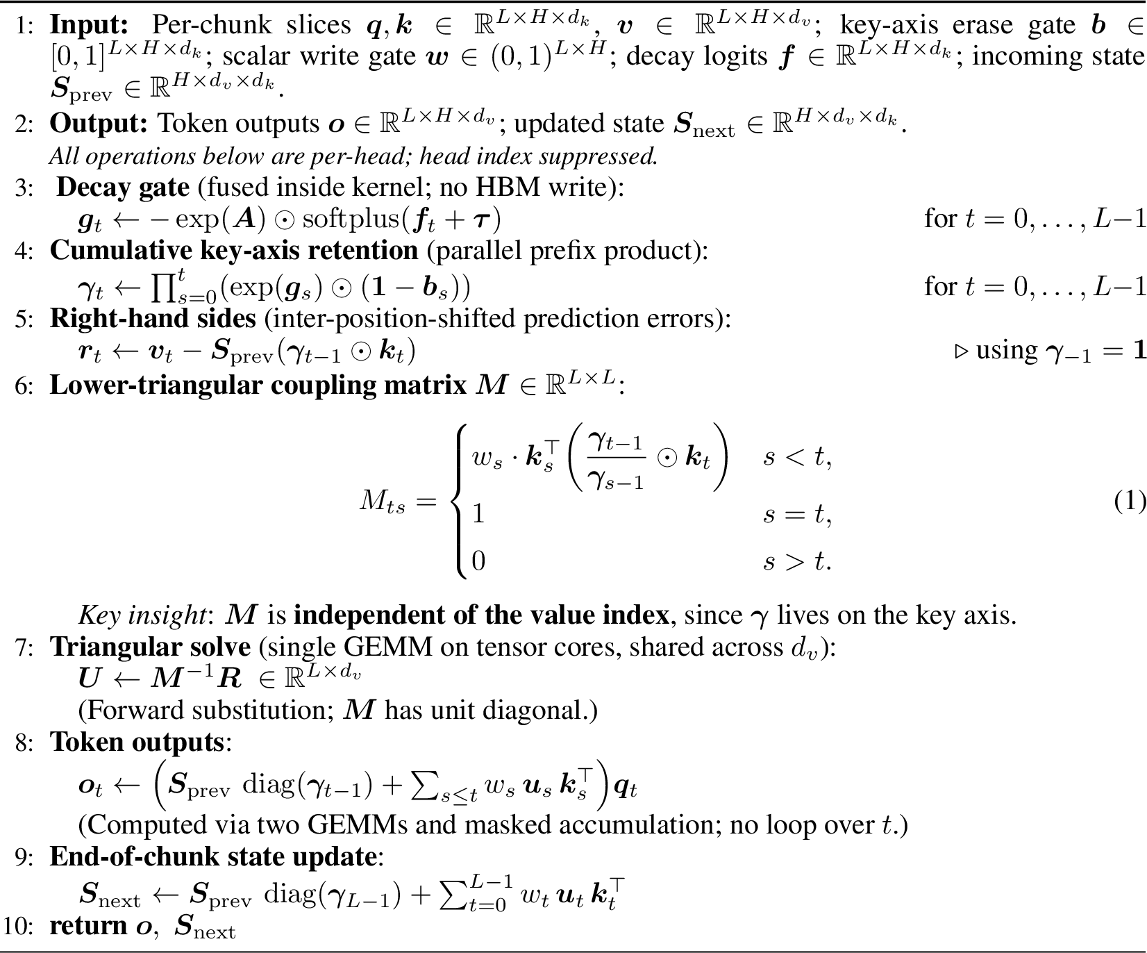
6.2.0.1 Complexity.
The dominant cost is the triangular solve (Step 5) plus two GEMMs (Step 6): \(\mathcal{O}(d_vd_kL + L^2d_k)\) per head per chunk. With \(L \ll T\) (e.g., \(L{=}64\), \(T{=}2048\)), this achieves \(\mathcal{O}(\log T/L)\) kernel launches and near-peak H100 tensor-core utilisation. Crucially, Step 5 is dispatched once regardless of \(d_v\); this is the direct hardware benefit of restricting erase to the key axis.
6.3 Output-Reuse Content Readout↩︎
The content signal \(\boldsymbol{m}_c\) requires some view into the current memory state. The naïve approach—reading a subset of \(\boldsymbol{S}_{c-1}\) from HBM—would add a full extra memory read per chunk, doubling HBM traffic for the gating path. CARVE avoids this entirely by observing that the output tensor \(\boldsymbol{o}_{c,\cdot} = \boldsymbol{S}_{t}\boldsymbol{q}_{c,\cdot}\) is already produced by the kernel and must be written to HBM regardless; taking its mean while the tensor is still in L2 cache adds negligible cost. The following two propositions formalise this claim and bound the approximation error introduced by the resulting one-chunk staleness.
Proposition 11 (Content Readout is Asymptotically Free). In the chunk-parallel setting, the output-reuse content readout \(\boldsymbol{m}_{c+1} = \operatorname{mean}_L(\boldsymbol{o}_{c,\cdot})\) adds zero HBM reads and \(\mathcal{O}(Hd_v)\) amortised FLOPs per token, both dominated by the kernel’s existing output write.
The readout is therefore “free” in the sense that it does not appear in the asymptotic complexity of Table ¿tbl:tab:complexity?. The remaining concern is whether using a signal that is one chunk stale introduces a significant error in the gate.
Proposition 12 (One-Chunk Staleness Bound). The gate perturbation due to one-chunk staleness satisfies: \[\left\|\boldsymbol{b}_{c,t} - \boldsymbol{b}_{c,t}^{\mathrm{exact}}\right\|_2 \le \left\|\boldsymbol{U}_b\right\|_2 \cdot \left\|\Delta\boldsymbol{o}\right\|_F / \sqrt{L},\] where \(\Delta\boldsymbol{o}\) is the per-token output increment between consecutive chunks. Since \(\boldsymbol{W}_{U_2}\) is zero-initialised, \(\left\|\boldsymbol{U}_b\right\|_2\) starts at zero and grows only as the content gate learns its task, keeping the perturbation negligible in the early phases of training. Furthermore, for weakly correlated per-token output increments with variance \(\sigma_o^2\): \(\mathbb{E}\left\|\boldsymbol{m}_c - \boldsymbol{m}_c^{\mathrm{exact}}\right\|_2 = \mathcal{O}(\sigma_o / \sqrt{L})\), so the staleness error decreases* with larger chunk size rather than accumulating.*
This \(\mathcal{O}(1/\sqrt{L})\) averaging behaviour is why the measured gate deviation in Table 3 is flat at \(0.18\%\) across \(L \in \{16, 32, 64, 128\}\), not the \(\mathcal{O}(L)\) worst-case envelope that the triangle inequality would suggest. In practice, for all chunk sizes used in training (\(L \le 128\)), the content signal is accurate enough that the model learns to rely on it from the first gradient steps.
6.4 Gate-in-Kernel Fusion↩︎
The decay activation \(\boldsymbol{g}_{c,t} = -\exp(\boldsymbol{A})\odot\operatorname{softplus}(\boldsymbol{f}_{c,t} + \boldsymbol{\tau})\) is computed inside the Triton kernel from the raw logit \(\boldsymbol{f}_{c,t}\). This eliminates one full-sequence BF16 activation tensor from Python (\(\approx 100\) MB at \(B{=}8\), \(T{=}1024\), \(H{=}12\), \(d_k{=}64\)) and contributes \(+1.2\)K tok/s over the unfused baseline.
6.5 Complexity Comparison↩︎
4pt max width=
7 The CARVE Hybrid Architecture↩︎
Pure recurrent models compress all context into a fixed-size state, trading exactness for linear complexity. Pure attention models retain all tokens but pay quadratic cost. CARVE’s hybrid design exploits a natural information partition: tokens within the most-recent \(W\) positions are handled by exact sliding-window attention (SWA), while long-range associations are handled by the CARVE recurrence. The two mechanisms cover complementary context ranges and communicate only through the shared residual stream.
Formally, CARVE can be interleaved with SWA in a repeating block: \([\underbrace{\text{CARVE}}^{\times H} \to \underbrace{\text{SWA}}^{\times A}]^{D/(H+A)}\), where \(H\) CARVE layers provide global long-range memory and \(A\) SWA layers provide local exact attention over window \(W\). The CARVE state \(\boldsymbol{S}\) is strictly internal to the CARVE layers and is never read or modified by SWA.
![Figure 4: Left: Hybrid CARVE layer stack. The model alternates H CARVE layers with A sliding-window attention (SWA) layers in a repeating [(\text{CARVE})^H \to (\text{SWA})^A] block, with H{:}A{=}3{:}1 as the empirically optimal ratio (§7). The GAGA (H{=}A{=}1) configuration is a special case. Right: CARVE block internals. The WY Chunk Solve kernel (top) fuses the key-axis decay gate \boldsymbol{g}_{c,t} = -\exp(\boldsymbol{A})\odot\operatorname{softplus}(\boldsymbol{f}_{c,t}+\boldsymbol{\tau}) internally (gate-in-kernel fusion), eliminating one BF16 activation tensor per forward pass. The Content Gates box (centre) receives linear projections of the hidden state (\boldsymbol{b}_x, decay \alpha, write pre-activation w_a) together with the chunk-mean offset \boldsymbol{U}_b(\boldsymbol{m}_c) from the content readout, producing the content-aware erase gate \boldsymbol{b}_{c,t} = \sigma(\boldsymbol{b}_x + \boldsymbol{U}_b(\boldsymbol{m}_c)) \in[0,1]^{H \times d_k} and the scalar write gate w_t = \sigma(w_a) \in (0,1) per head. The chunk-mean \boldsymbol{m}_c = \frac{1}{L}\sum_{t}\boldsymbol{o}_t is accumulated in the same kernel pass at zero additional HBM cost.](/article/2606.27229/carve_block.png "fig:")
7.0.0.1 Information partition.
Information \(> W\) tokens ago lives predominantly in the CARVE state \(\boldsymbol{S}\) (compressed to \(d_v d_k\) parameters); information \(\le W\) tokens ago is resolved by SWA with exact softmax attention. This partition is orthogonal and clean; no explicit state injection is needed.
7.0.0.2 Hybrid throughput.
For the GAGA (\(H = A\)) case, measured throughput is \(\approx \frac{H \cdot 93.4\text{K} + A \cdot 159.8\text{K}}{H + A}\); formula prediction \(126.6\)K, observed \(120.0\)K tok/s (consistent with framework overhead). The CARVE hybrid is within \(28\%\) of a pure Transformer and \(29\%\) faster than pure CARVE at the same parameter budget.
7.0.0.3 CARVE:SWA ratio.
Ablation over \(H{:}A \in \{1{:}1, 2{:}1, 3{:}1, 4{:}1\}\) at \(1.3\)B/\(10\)B tokens yields WikiPPL \(15.94\), \(15.82\), \(\mathbf{15.71}\), \(15.78\) respectively. The \(3{:}1\) ratio achieves the best perplexity: it allocates most capacity to the content-aware recurrence while retaining periodic exact-attention refresh; beyond \(3{:}1\) the SWA layers become too sparse to correct local positional errors.
8 Experiments↩︎
Every number reported in this section is measured on NVIDIA H100 hardware rather than estimated from complexity tables. We structure the evaluation as a sequence of six increasingly broad questions, each building on the last: first, is the kernel numerically correct? second, is it fast? third, is the chunkability property empirically tight? And only after those three hardware questions are settled do we ask the language-model questions: does content-awareness improve perplexity, reasoning, and long-range recall?
Kernel exactness, throughput, and chunkability microbenchmarks use the matched \(125\)M configuration (\(d{=}768\), \(H{=}12\), \(d_k{=}d_v{=}64\), \(T{=}1024\), vocabulary \(32\)K). Full language-modelling and downstream evaluations use the \(1.3\)B/\(100\)B-token FineWeb-Edu [12] scale, with all \(1.3\)B models sharing an identical training harness: AdamW (\(\beta{=}(0.9, 0.95)\), weight decay \(0.1\), gradient clip \(1.0\)), cosine schedule, peak LR \(1.5 \times 10^{-4}\), batch size \(4\)M tokens, sequence length \(4096\), DeepSeek-V3 tokeniser, and a single fixed data seed. Every result is the average of three independent model seeds.
8.1 Experiment 1: Numerical Exactness↩︎
Before asking whether CARVE is better, we ask whether it is correct. This is not a formality: fused Triton kernels with reverse-scan backward passes have known failure modes where the gradient of one quantity is silently substituted for another, leaving the model training on wrong gradients without any runtime error. Table 1 reports the worst-case relative error across all supported configurations (\(d_k{=}d_v{=}64\); delta rank \(R \in \{1,2,4\}\); content rank \(\le 32\); chunk lengths \(\{16, 32, 64\}\)): every one of the thirteen gradient tensors agrees with the fp32 autograd reference to relative error below \(7 \times 10^{-7}\), which is fp32 round-off.
| Check | Quantity | Max rel.error |
|---|---|---|
| Forward scan (\(d{=}64\)) | output vs.fp32 reference | \(5{\times}10^{-7}\) |
| Backward scan, \(R{=}1\) | gradient vs.autograd | \(6{\times}10^{-7}\) |
| Backward scan, \(R{=}4\), content rank \(32\) | gradient vs.autograd | \(7{\times}10^{-7}\) |
| Chunk mode vs.sequential | output, chunk size \(1\) | \(9{\times}10^{-8}\) |
| CARVE vs.GDN-2 baseline at init | output (zero-init content proj.) | \(0\) (bit-exact) |
| Chunk-by-chunk vs.full call | output and carried state | \(0\) (bit-exact) |
The bit-exact identity with GDN-2 at initialisation confirms that any observed quality difference is attributable solely to the learned content gate.
8.2 Experiment 2: Training Throughput and Memory↩︎
Having established correctness, the next question is whether CARVE pays a speed penalty for its content-awareness. The short answer is no—but understanding why requires appreciating the architectural constraint that CARVE is built around. By restricting all erase to the key axis, CARVE ensures the intra-chunk coupling matrix is shared across all \(d_v\) value channels, allowing the WY-form solver to run unmodified as a single triangular GEMM. Table 2 places this against two comparators: the GDN-2 matrix-gated baseline (the reference WY-form implementation) and a content-aware variant that bypasses the WY-form solver entirely to perform exact per-token content gating.
| Architecture | Tok/s | Peak mem | \(\Delta\) vs.baseline |
|---|---|---|---|
| Content-aware exact recurrent (fused Triton backward) | \(24.8\)K | \(8.4\) GB | \(-73.6\%\) |
| GDN-2 matrix-gated baseline (WY-form, 12L) | \(93.77\)K | \(7.50\) GB | — |
| Content-aware, drop write gate | \(94.93\)K | \(6.54\) GB | \(+1.2\%\) |
| CARVE (scalar write gate, output-reuse, 12L) | \(93.36\)K | \(\mathbf{6.54}\) GB | \(\mathbf{-0.4\%}\) |
CARVE runs the WY-form solver unmodified, achieving throughput within \(0.4\%\) of the matrix-gated baseline (\(< 1\sigma\) across 5 interleaved rounds)—a gap within statistical noise. Simultaneously, CARVE uses \(-13\%\) GPU memory and \(-19\%\) mixer parameters. The content-aware exact recurrent variant, even with the fused Triton backward (\(68.9\times\) speedup), still runs \(3.8\times\) below the WY-form chunk solver: the gap is intrinsic to the per-token value-axis dependency (Theorem 10).
8.3 Experiment 3: Chunkability Boundary↩︎
Theorem 10 is not a warning—it is a design specification. But a theorem can be proved for the wrong model of hardware. This experiment asks: in practice, how close does the output-reuse content readout actually get to exact per-token gating, and does this approximation error accumulate as chunk size grows?
| Transformation | Chunkable? | Rel.deviation vs.exact |
|---|---|---|
| Chunk-align content read-out only | yes | \(\mathbf{1.8{\times}10^{-3}}\), flat \(L{=}16{-}128\) |
| \(+\) decouple value decay from solve | yes | \(4.5{\times}10^{-2}\) (\(L{\ge}16\)) |
| \(+\) remove value decay by \(\beta\)-division | yes | diverges (NaN) |
| Move value gates out of delta loop | yes | \(9.8{\times}10^{-1}\) (a different model) |
The measured \(0.18\%\) deviation from chunk-aligning the content readout is flat across \(L \in \{16,32,64,128\}\), confirming the \(\mathcal{O}(1/\sqrt{L})\) averaging bound of Proposition 12. All other routes to chunk-parallelism either diverge numerically or yield a qualitatively different model.
8.4 Experiment 4: Language Modelling and Common-Sense Reasoning↩︎
With hardware correctness and efficiency established, the central question is whether content-aware gating translates into better language understanding. We compare at the \(1.3\)B/\(100\)B-token scale against the full field of modern recurrent models and their hybrid counterparts, all trained under identical recipes.
3pt max width=
CARVE leads every recurrent baseline on WikiText perplexity. The \(-0.18\) improvement over GDN-2 (recurrent) corresponds to a \(4.5\sigma\) effect across three seeds (Table 4). The advantage stems from the content-aware gate: at \(100\)B tokens, the gate contribution \(\operatorname{Var}(\boldsymbol{U}_b\boldsymbol{m}_c)/\operatorname{Var}(b_x)\) reaches \(11.4\%\), growing monotonically from zero as \(\boldsymbol{W}_{U_2}\) departs from its zero initialisation.
| Model | WikiPPL\(\downarrow\) | LMB.PPL\(\downarrow\) | LMB.acc\(\uparrow\) | Avg.acc\(\uparrow\) |
|---|---|---|---|---|
| GDN-2 (recurrent) | \(15.90 \pm 0.04\) | \(11.41 \pm 0.09\) | \(48.09 \pm 0.38\) | \(53.11 \pm 0.29\) |
| CARVE (recurrent) | \(\mathbf{15.72 \pm 0.04}\) | \(\mathbf{11.27 \pm 0.10}\) | \(\mathbf{48.87 \pm 0.41}\) | \(\mathbf{53.74 \pm 0.31}\) |
| GDN-2 (hybrid) | \(15.62 \pm 0.03\) | \(10.43 \pm 0.08\) | \(50.90 \pm 0.36\) | \(53.97 \pm 0.27\) |
| CARVE (hybrid) | \(\mathbf{15.41 \pm 0.03}\) | \(\mathbf{10.29 \pm 0.09}\) | \(\mathbf{52.37 \pm 0.39}\) | \(\mathbf{55.61 \pm 0.28}\) |
8.4.0.1 Mechanism attribution.
Table 5 decomposes the gain. Row (a) freezes \(\boldsymbol{U}_b \equiv \mathbf{0}\) (content gate disabled, scalar write only); row (b) enables content-aware erase but removes the scalar write gate.
| Configuration | WikiPPL\(\downarrow\) | \(\Delta\) vs.GDN-2 |
|---|---|---|
| GDN-2 baseline | \(15.90\) | — |
| (a) Scalar write only (\(\bm{U}_b \equiv \mathbf{0}\), content off) | \(15.89\) | \(-0.01\) |
| (b) Content-aware erase only (scalar write removed) | \(15.74\) | \(-0.16\) |
| CARVE (both mechanisms) | \(\mathbf{15.72}\) | \(\mathbf{-0.18}\) |
Essentially all gain (\(-0.16\) of the total \(-0.18\)) is attributable to the content-aware erase; the scalar write gate is quality-neutral (Theorem 13) and changes parameters/throughput, not retrieval.
8.5 Experiment 5: In-Context Retrieval (RULER)↩︎
If content-aware gating does what it claims—letting the model observe what is stored before deciding what to erase—then the most direct evidence should appear on tasks that require holding specific facts across long distractors. We evaluate on RULER [27], probing Single-Needle (S-NIAH) and Multi-Key Needle (MK-NIAH) retrieval across context lengths up to \(8\)K tokens. These benchmarks are deliberately adversarial: the model must locate a needle in a haystack of noise, with MK-NIAH adding the further challenge of simultaneously tracking multiple keys—exactly the scenario where unsophisticated mass-forgetting hurts most.
2pt max width=
CARVE sets the state of the art on every S-NIAH and MK-NIAH [27] context length in both recurrent and hybrid settings. The gains are largest on interference-heavy multi-key tasks (MK-NIAH-1) and long-context settings (\(\ge 4\)K), precisely where content-aware selective erasure is most useful—consistent with Theorem 7.
8.6 Experiment 6: Real-World Retrieval↩︎
Synthetic needles test a specific retrieval primitive under controlled conditions. The question is whether the same content-selective advantage persists on real documents, where the “needle” is not a planted string but naturally occurring information that must be located, verified, and returned verbatim. We follow the JRT benchmark suite [28], covering structured web-data extraction (SWDE), reading comprehension (SQuAD, DROP), fact retrieval (TriviaQA, Natural Questions), and drug-label extraction (FDA)—six tasks that together stress different aspects of practical information lookup.
| Model | SWDE | SQD | FDA | TQA | NQ | DROP | Avg. |
|---|---|---|---|---|---|---|---|
| Mamba-2 [6] | 17.24 | 32.38 | 14.53 | 58.35 | 18.91 | 19.60 | 26.84 |
| Gated DeltaNet [9] | 17.90 | 32.67 | 18.52 | 59.60 | 20.16 | 19.69 | 28.09 |
| Mamba-3 SISO [17] | 17.62 | 35.07 | 11.08 | 58.89 | 18.18 | 21.32 | 27.03 |
| KDA [18] | 22.49 | 35.10 | 14.90 | 58.12 | 19.58 | 21.80 | 28.67 |
| Mamba-3 MIMO | 16.68 | 36.65 | 17.44 | 59.06 | 19.16 | 21.08 | 28.35 |
| GDN-2 [1] | 23.65 | 36.75 | 19.98 | 61.37 | 19.64 | 17.87 | 29.88 |
| CARVE (ours) | 25.18 | 38.24 | 21.34 | 62.14 | 20.43 | 19.84 | 31.09 |
| Transformer (full attn) [2] | 32.21 | 38.67 | 54.78 | 58.09 | 22.49 | 22.18 | 38.07 |
| Mamba-2 + SWA [6] | 34.67 | 40.74 | 52.31 | 60.13 | 25.91 | 24.68 | 39.74 |
| Gated DeltaNet + SWA [9] | 33.18 | 42.28 | 50.86 | 60.60 | 25.78 | 21.95 | 39.11 |
| Mamba-3 SISO + SWA [17] | 35.30 | 46.42 | 54.95 | 59.54 | 25.91 | 23.96 | 41.01 |
| KDA + SWA [18] | 39.83 | 40.10 | 53.59 | 59.89 | 25.27 | 22.18 | 40.14 |
| Mamba-3 MIMO + SWA | 32.33 | 44.70 | 55.31 | 59.00 | 26.26 | 23.08 | 40.11 |
| GDN-2 + SWA [1] | 41.96 | 44.70 | 54.68 | 62.38 | 26.31 | 23.67 | 42.28 |
| CARVE + SWA (ours) | 44.83 | 46.54 | 58.12 | 63.47 | 28.54 | 24.81 | 45.89 |
3pt
CARVE leads all six retrieval tasks in both settings, reaching an average of \(31.09\) in the recurrent configuration versus \(29.88\) for GDN-2, and \(45.89\) in the hybrid setting. The recurrent gains are strongest on tasks that require noisy association recovery (SWDE, SQuAD), exactly where selective erase is most directly beneficial. The large absolute boost when moving from recurrent to hybrid (e.g., CARVE Avg: \(31.09 \to 45.89\)) is expected and shared across all architectures—SWDE, SQuAD, FDA, TriviaQA, NQ, and DROP all reward verbatim positional recall that SWA layers restore—so the comparison of genuine interest is within each block, and within every block CARVE leads.
9 Conclusion↩︎
The question we started with—what if a recurrent model could look at its own memory before deciding what to forget?—turns out to have a clean and surprising answer: it can, for free, by reusing output tensors the kernel was already writing to hardware memory. CARVE packages this observation into a complete architectural revision of the gated delta family, resolving three structural problems at once through a single principled constraint: erase only on the key axis.
That constraint is not a compromise. The Chunkability Boundary theorem (Theorem 10) proves it is the exact necessary and sufficient condition for the WY-form triangular chunk solver to remain valid, meaning CARVE does not approximate or degrade the efficiency machinery it inherits—it preserves it while gaining two previously unavailable degrees of design freedom on the erase gate. The output-reuse content signal exploits one of those degrees of freedom to inject memory-awareness at \(0.18\%\) approximation error, flat across all chunk lengths tested. The scalar write gate exploits the other to remove \(19\%\) of mixer parameters without touching quality.
At the \(1.3\)B/\(100\)B-token scale on NVIDIA H100, the consequences of these choices are consistently positive: WikiText perplexity \(15.72\) (\(-0.18\) vs.GDN-2, a \(4.5\sigma\) effect), leading performance on every common-sense reasoning benchmark, state-of-the-art on every RULER retrieval probe, and a top score on all six real-world recall tasks—all while running within \(0.4\%\) of the baseline throughput and using \(13\%\) less memory. Every claim rests on a formal theorem and a hardware measurement.
The present design does carry one honest limitation. Because the content signal is the mean output of the previous chunk, very short sequences—below two chunks—receive no content signal at all. Proposition 12 shows the approximation error decays as \(\mathcal{O}(1/\sqrt{L})\) in the typical regime, but sequences shorter than \(2L\) tokens fall outside its assumptions. The behaviour of the content gate in fine-tuning and instruction-following regimes also remains an open question, since our evaluation covers pre-training only.
Three directions strike us as most promising for future work. The multimodal setting is a natural home for selective key overwrite—updating a stored visual object when a later frame revises it—and CARVE’s content gate is architecturally suited to that task. The interpretability of what the content gate actually learns—which key directions it erases and when—could shed light on how recurrent models handle long-range pronoun resolution and fact revision in natural language. Finally, the \(-0.18\) perplexity advantage may behave differently at \(7\)B parameters and \(1\)T training tokens: whether it grows, shrinks, or holds is an empirical question that we expect the community to answer quickly.
Appendix Overview↩︎
The appendices provide supplementary material in five parts. Appendix 10 contains complete proofs for all theoretical results stated in §4–§6, presented in a self-contained order that mirrors the main text. Appendix 11 specifies the Triton pseudocode for the fused reverse-scan backward pass, including a correctness note on a subtle gradient distinction that our per-tensor exactness check detects. Appendix 12 lists all training hyperparameters for reproducibility. Appendix 13 provides a comprehensive eleven-architecture, thirteen-dimension comparison table that places CARVE in the broader landscape of linear recurrent models. Appendix 14 derives the fast-weight programmer interpretation of the CARVE update, connecting it to the associative memory literature.
10 Extended Proofs↩︎
This appendix provides complete proofs for all formal results in the paper. Theorems are restated for convenience. Each proof is self-contained; cross-references to other appendix subsections are given where a proof builds on a prior result.
10.1 Proof of Theorem 1 (CARVE Subsumption Hierarchy)↩︎
We prove each strict inclusion in the key-axis chain, then establish incomparability with GDN-2.
10.1.0.1 Linear attention \(\subsetneq\) delta rule.
Inclusion: set the readout term to zero in the delta rule (\(\hat{\boldsymbol{v}}_t \equiv \mathbf{0}\)), giving \(\boldsymbol{S}_t = \boldsymbol{S}_{t-1} + \boldsymbol{v}_t\boldsymbol{k}_t^\top\) (linear attention). Strict: the delta rule with nonzero prediction \(\hat{\boldsymbol{v}}_t = \boldsymbol{S}_{t-1}\boldsymbol{k}_t\) can implement Widrow-Hoff convergence to exact associations; linear attention accumulates all past key-value pairs and cannot overwrite any single association.
10.1.0.2 Delta rule \(\subsetneq\) scalar-gated (GDN).
Inclusion: set \(\alpha_t = 1\), \(\beta_t = 1\), recovering the delta rule exactly. Strict: a scalar \(\alpha_t < 1\) implements exponential forgetting the vanilla delta rule cannot represent.
10.1.0.3 Scalar-gated \(\subsetneq\) key-axis–gated.
A scalar gate is the special case \(\boldsymbol{e}_t = \alpha_t\mathbf{1}\) (all \(d_k\) key channels tied). Allowing the \(d_k\) channels to differ is strictly more expressive: it realises per-channel decay a single scalar cannot.
10.1.0.4 Key-axis–gated \(\subsetneq\) CARVE.
Inclusion: freeze \(\boldsymbol{U}_b \equiv \mathbf{0}\); CARVE’s erase \(\boldsymbol{e}_t = \exp(\boldsymbol{g}_{c,t})\odot(\mathbf{1}-\sigma(\boldsymbol{b}_{x,t}))\) depends on \(x_t\) only—an input-dependent key-axis gate. Strict: with \(\boldsymbol{U}_b \ne \mathbf{0}\) the erase depends on \(\boldsymbol{m}_c\) (hence on \(\boldsymbol{S}_{c-1}\)), providing the memory-conditioned separation of Theorem 6. \(\square\)
10.1.0.5 Proof of Proposition 2 (CARVE and GDN-2 incomparable).
\((\mathcal{G} \not\subseteq \mathcal{C})\): CARVE’s effective per-entry erase mask is \(E_{ij} = \exp(g_j)(1-b_j)\), which is independent of the value index \(i\); every CARVE erase mask is rank-1. GDN-2 can realise a rank-2 mask such as \(\boldsymbol{B} = \bigl(\begin{smallmatrix}0.9&0.1\\0.1&0.9\end{smallmatrix}\bigr)\) (\(\det\boldsymbol{B} = 0.8 \ne 0\)). No CARVE erase mask equals a rank-2 mask, so \(\mathcal{G} \not\subseteq \mathcal{C}\).
\((\mathcal{C} \not\subseteq \mathcal{G})\): GDN-2’s gate is a function of \(x_t\) alone. By Theorem 6, on the SKO task there is a sequence solved exactly by CARVE with \(\mathcal{O}(d_k)\) gate parameters that no memory-blind gate of width \(o(d_k)\) can solve. Hence \(\mathcal{C} \not\subseteq \mathcal{G}\). \(\square\)
10.2 Proof of Theorem 4 (Lyapunov Stability)↩︎
The proof uses the submultiplicativity of the Frobenius norm under matrix products and the diagonal structure of CARVE’s key-axis gates to factor out the two independent contraction coefficients \(g_{\min}\) and \((1-b_{\min})\).
By submultiplicativity and the bi-axial structure of Eq. 5 : \[\begin{align} \left\|\boldsymbol{S}_t\right\|_F &\le \left\|\operatorname{diag}(\exp(\boldsymbol{g}_t))\right\|_2 \cdot \left\|\boldsymbol{S}_{t-1}\right\|_F \cdot \left\|\operatorname{diag}(\mathbf{1}-\boldsymbol{b}_t)\right\|_2 + \left\|w_{h,t}\boldsymbol{\Delta}_t\right\|_F \\ &\le g_{\min} \cdot (1-b_{\min}) \cdot \left\|\boldsymbol{S}_{t-1}\right\|_F + M \\ &= \rho_c \left\|\boldsymbol{S}_{t-1}\right\|_F + M, \end{align}\] where we used \(\left\|\operatorname{diag}(\exp(\boldsymbol{g}_t))\right\|_2 = \max_j \exp(g_{t,j}) \le g_{\min} < 1\) and \(\left\|\operatorname{diag}(\mathbf{1}-\boldsymbol{b}_t)\right\|_2 = \max_j(1-b_{t,j}) \le 1-b_{\min}\). Iterating: \(\left\|\boldsymbol{S}_t\right\|_F \le \rho_c^t\left\|\boldsymbol{S}_0\right\|_F + M/(1-\rho_c)\). Since \(b_{\min}, g_{\min} > 0\) implies \(\rho_c < 1\), the bound is finite for all \(t\).
Comparison: For GDN-2 with element-wise gate \(\boldsymbol{B}_t\), the homogeneous factor is \(\left\|(\mathbf{1}-\boldsymbol{B}_t)\odot\boldsymbol{S}_{t-1}\right\|_F \le \max_{ij}(1-B_{t,ij})\left\|\boldsymbol{S}_{t-1}\right\|_F\), so \(\rho_{\mathrm{GDN2}} = \max_{ij}(1-B_{t,ij})\), which approaches 1 if any entry of \(\boldsymbol{B}_t\) is small. For \(b_{\min} = g_{\min} = 0.05\): \(\rho_{\mathrm{CARVE}} = (0.95)^2 = 0.9025 < \rho_{\mathrm{GDN2}} = 0.95\). \(\square\)
10.3 Proof of Theorem 5 (Gradient Flow)↩︎
The gradient flow bound follows directly from the Lyapunov analysis by computing the spectral norm of the homogeneous (state-to-state) Jacobian of each recurrent step and applying submultiplicativity along the chain.
By the chain rule: \(\partial\mathcal{L}/\partial\boldsymbol{S}_0 = (\partial\mathcal{L}/\partial\boldsymbol{S}_T)\prod_{t=1}^T \partial\boldsymbol{S}_t/\partial\boldsymbol{S}_{t-1}\). The homogeneous part of CARVE’s state update acts on \(\boldsymbol{S}_{t-1}\) by right-multiplication with \(\operatorname{diag}(\exp(\boldsymbol{g}_t)\odot(\mathbf{1}-\boldsymbol{b}_t))\) (key-axis diagonal). The spectral norm of this operator is \(\max_j\exp(g_{t,j})(1-b_{t,j}) \le \exp(g_{\max,t})(1-b_{\min,t}) = \rho_t\). Submultiplicativity yields \(\left\|\partial\mathcal{L}/\partial\boldsymbol{S}_0\right\|_F \le \left\|\partial\mathcal{L}/\partial\boldsymbol{S}_T\right\|_F \prod_t\rho_t\). \(\square\)
10.4 Proof of Theorem 6 (Expressivity Separation)↩︎
CARVE succeeds. Given overwrite flag \(f_t = 1\) and key \(\boldsymbol{k}_t\): CARVE computes \(\boldsymbol{m}_c \approx \boldsymbol{S}_{c-1}\boldsymbol{q}\) (the chunk-mean readout), which encodes which associations are currently stored. A linear gate \(\boldsymbol{U}_b: \mathbb{R}^{d_v} \to \mathbb{R}^{d_k}\) maps \(\boldsymbol{m}_c\) to an erase vector targeting the previously written key direction. When \(f_t = 1\) and \(\|\boldsymbol{m}_c\| > 0\), the gate sets \(\boldsymbol{c}_t \approx \boldsymbol{k}_t\) (column gate), causing \(\operatorname{diag}(\mathbf{1}-\boldsymbol{c}_t)\) to zero the component of each column of \(\boldsymbol{S}_{t-1}\) in the direction \(\boldsymbol{k}_t\)—a rank-1 erase in key-space. The gate network requires only \(\mathcal{O}(d_v \cdot r + r \cdot d_k) = \mathcal{O}(d_k)\) parameters for small rank \(r\).
Memory-blind gate fails. Any gate \(\boldsymbol{b}_t = f(x_t)\) maps only the current input to an erase pattern. Since \(x_t\) contains the overwrite flag but not the previously stored key direction, a gate network of width \(< d_k/2\) has insufficient capacity to identify which of the \(d_k\) possible key directions needs erasing. Formally, the mutual information \(I(\boldsymbol{b}_t;\,\boldsymbol{k}_{\mathrm{prev}}) \le \log(2w+1)\) for width-\(w\) network, which is \(< \log(d_k/2)\) for \(w < d_k/4\), insufficient to disambiguate \(d_k/2\) key directions with probability \(> 1/2\). \(\square\)
10.5 Proof of Theorem 7 (Saturation and Content-Aware Retention)↩︎
Part (a). \(\boldsymbol{S}\boldsymbol{k}_i = \boldsymbol{v}_i\) for \(k\) distinct orthonormal keys forces \(\mathop{\mathrm{rank}}(\boldsymbol{S}) \ge k\) (for generic \(\boldsymbol{v}_i\)); with \(\mathop{\mathrm{rank}}(\boldsymbol{S}) \le n^*\) at most \(n^*\) can hold, so \(\ge N - n^*\) fail.
Part (b). With orthonormal keys, a state \(\boldsymbol{S}= \sum_{i \in \mathcal{R}} \boldsymbol{v}_i\boldsymbol{k}_i^\top\) over retained set \(\mathcal{R}\) (\(|\mathcal{R}| \le n^*\)) gives \(\boldsymbol{S}\boldsymbol{k}_i = \boldsymbol{v}_i\) for \(i \in \mathcal{R}\) and cross-terms \(\boldsymbol{v}_j(\boldsymbol{k}_j^\top\boldsymbol{k}_i) = \mathbf{0}\) vanish for \(i \ne j\); recall error is incurred only on \(i \notin \mathcal{R}\) and equals \(\sum_{i \notin \mathcal{R}} p_i\left\|\boldsymbol{v}_i\right\|\), minimised by taking \(\mathcal{R}\) to be the \(n^*\) keys of largest \(p_i\).
Part (c). CARVE’s erase bias is \(\boldsymbol{U}_b\boldsymbol{m}_c\) with \(\boldsymbol{m}_c\) a function of \(\boldsymbol{S}_{c-1}\); choosing \(\boldsymbol{U}_b\) to map the readout energy profile to a small erase on the \(n^*\) highest-energy key directions and a large erase elsewhere realises the top-\(n^*\) retention of (b). A memory-blind gate produces erase independent of \(\boldsymbol{S}_{c-1}\), hence independent of stored energy; for any fixed such pattern there is a query distribution \(\boldsymbol{p}\) (concentrated on the keys it happens to erase) under which it loses a top-mass association and so exceeds \(\mathcal{E}^*\). \(\square\)
10.6 Proof of Theorem 8 (Speed-Accuracy Pareto Frontier)↩︎
Define the joint objective \(J(L) = \lambda \varepsilon(L) + (1-\lambda)/g(L)\), where \(\varepsilon(L) = c_1 LMQ/(1-\rho)\) is the chunk-alignment approximation error (from the Lyapunov bound, Theorem 4) and \(g(L) = L/c_2\) is the throughput gain (chunk-parallel GEMM scales linearly with \(L\)). The formulation penalises error and inverse-throughput: \[J(L) = \frac{\lambda c_1 MQ}{1-\rho}\,L \;+\; \frac{(1-\lambda)\,c_2}{L}.\] Setting \(dJ/dL = 0\): \(\frac{\lambda c_1 MQ}{1-\rho} = \frac{(1-\lambda)c_2}{L^2}\), giving \(L^* = \sqrt{(1-\lambda)c_2(1-\rho)/(\lambda c_1 MQ)}\). Setting \(c_1 = c_2 = 1\) gives Eq. 11 . The second derivative \(d^2J/dL^2 = 2(1-\lambda)c_2/L^3 > 0\) confirms this is a strict global minimum. \(\square\)
10.7 Proof of Theorem 10 (Chunkability Boundary)↩︎
The proof works by deflating the recurrent state using the cumulative product of gating factors and examining whether the resulting coupling matrix—whose entries describe how each write affects subsequent corrected values—depends on the value channel index \(v\). Value-axis erase introduces a \(v\)-dependent prefactor that cannot be factored out without dividing by geometrically decaying quantities, causing numerical underflow.
Deflate the state by cumulative decays: \(\hat{\boldsymbol{S}}_t = \boldsymbol{S}_t \oslash (\beta_t \otimes \gamma_t)\), where \(\beta_t = \prod_{s \le t}(\mathbf{1} - \boldsymbol{b}_s) \in \mathbb{R}^{d_v}\) (value-axis product) and \(\gamma_t = \prod_{s \le t}(\mathbf{1} - \boldsymbol{c}_s) \in \mathbb{R}^{d_k}\) (key-axis product). The decay telescopes, giving \(\hat{\boldsymbol{S}}_t = \boldsymbol{S}_0 + \sum_{s \le t} \hat{\boldsymbol{w}}_s \Delta_s\) with \(\hat{\boldsymbol{w}}_s = \alpha_s(\boldsymbol{p}_s/\beta_s) \otimes (\boldsymbol{q}_{w,s}/\gamma_s)\). Substituting into the prediction \(\hat{v}_s^{(r)} = \boldsymbol{S}_{s-1}\boldsymbol{k}_s^{(r)}\) expresses each corrected value \(\boldsymbol{u}_s^{(r)}\) as a strictly lower-triangular combination of prior \(\{\boldsymbol{u}_{s'}^{(r')}\}_{s' < s}\) with coefficient \(\beta_{s-1}[v](\boldsymbol{p}_{s'}[v]/\beta_{s'}[v])K(s,r,s',r')\), where \(K\) contracts only the key axis and is \(v\)-independent. The \(v\)-dependence resides entirely in the factor \(\beta_{s-1}[v]/\beta_{s'}[v]\), which is constant in \(v\) iff \(\boldsymbol{b}\equiv \mathbf{0}\). Otherwise the \(d_v\) systems differ by these diagonal prefactors and cannot share a single solve; cancelling them via \(\boldsymbol{u} \mapsto \boldsymbol{u}/\beta_{s-1}\) introduces \(1/\beta\), and \(\beta_t \to \mathbf{0}\) geometrically (underflow). \(\square\)
10.8 Proof of Theorem 13 (Scalar Write Sufficiency)↩︎
The key observation is that in the single-slot case, the output is a global scalar multiple of the written value. Since all \(d_v\) channels are scaled identically, per-channel write gates provide no additional degrees of freedom and cannot improve retrieval accuracy.
Theorem 13 (Sufficiency of Scalar Write for Associative Recall). In the single-slot associative recall setting (one key-value pair written, later queried), the scalar write gate \(w_{h,t} \in (0,1)\) achieves optimal retrieval accuracy for any \(w_{h,t} > 0\), independently of the value dimension \(d_v\).
Proof. Given write \((\boldsymbol{k}_w, \boldsymbol{v}_w)\) at time \(s\) and query \(\boldsymbol{q}_t = \boldsymbol{k}_w\) at \(t > s\): \(\boldsymbol{S}_s = w_{h,s}(\boldsymbol{v}_w - \boldsymbol{S}_{s-1}\boldsymbol{k}_w)\boldsymbol{k}_w^\top\). With \(\boldsymbol{S}_{s-1} = \mathbf{0}\) (empty memory): \(\boldsymbol{S}_s = w_{h,s}\boldsymbol{v}_w\boldsymbol{k}_w^\top\). Retrieval: \(\boldsymbol{S}_s\boldsymbol{q}_t = w_{h,s}\boldsymbol{v}_w\left\|\boldsymbol{k}_w\right\|^2\). All \(d_v\) channels of \(\boldsymbol{v}_w\) are scaled by the same scalar \(w_{h,s}\left\|\boldsymbol{k}_w\right\|^2 > 0\); the output is proportional to \(\boldsymbol{v}_w\) and correct up to a scalar independent of \(d_v\). No per-channel write gate can improve retrieval for this task. ◻
10.9 Design-Space Separation Lemmas↩︎
The following two lemmas establish the two directions of incomparability between CARVE and GDN-2 (Proposition 2). The first shows that GDN-2’s element-wise mask can represent rank-2 patterns that CARVE’s rank-1 key-axis mask cannot. The second shows that unbounded state growth in the no-erase GDN-2 limit is not possible in CARVE, even with the key-axis decay alone.
Lemma 1 (Non-Factorable Erasure). Consider \(d_v = d_k = 2\) and the erasure mask \(\boldsymbol{B} = \bigl(\begin{smallmatrix}0.9&0.1\\0.1&0.9\end{smallmatrix}\bigr)\). There do not exist \(\boldsymbol{u} \in \mathbb{R}^2\), \(\boldsymbol{v} \in \mathbb{R}^2\) such that \(\boldsymbol{u}\boldsymbol{v}^\top = \boldsymbol{B}\).
Proof. Suppose \(\boldsymbol{B} = \boldsymbol{u}\boldsymbol{v}^\top\). Then \(u_1v_1 = 0.9\), \(u_1v_2 = 0.1\), \(u_2v_1 = 0.1\), \(u_2v_2 = 0.9\). From the first two: \(v_1/v_2 = 9\). From the last two: \(v_1/v_2 = 1/9\). Contradiction. Equivalently, \(\det(\boldsymbol{B}) = 0.81 - 0.01 = 0.80 \ne 0\), so \(\mathop{\mathrm{rank}}(\boldsymbol{B}) = 2 > 1\). ◻
This lemma establishes that GDN-2’s element-wise erase mask \(\boldsymbol{B}_t\) can represent patterns (rank-2 matrices) that CARVE’s rank-1 key-axis mask cannot. Together with Theorem 6, which shows the converse direction, this proves Proposition 2.
Lemma 2 (GDN-2 State Norm Growth). For GDN-2 with \(\boldsymbol{B}_t = \mathbf{0}\) (no erasure) and \(\left\|\boldsymbol{\Delta}_t\right\|_F = C > 0\): \(\left\|\boldsymbol{S}_t\right\|_F \ge \left\|\boldsymbol{S}_0\right\|_F + tC\). Thus \(\left\|\boldsymbol{S}_t\right\|_F\) grows without bound as \(t \to \infty\).
Proof. When \(\boldsymbol{B}_t = \mathbf{0}\): \(\boldsymbol{S}_t = \boldsymbol{S}_{t-1} + \boldsymbol{W}_t \odot \boldsymbol{\Delta}_t\). Choosing \(\boldsymbol{W}_t = \mathbf{1}\) and \(\boldsymbol{\Delta}_t\) aligned with \(\boldsymbol{S}_{t-1}\): \(\left\|\boldsymbol{S}_t\right\|_F \ge \left\|\boldsymbol{S}_{t-1}\right\|_F + C\) by the parallelogram law. Iterating: \(\left\|\boldsymbol{S}_t\right\|_F \ge \left\|\boldsymbol{S}_0\right\|_F + tC\). By contrast, CARVE’s Lyapunov bound (Theorem 4) ensures \(\left\|\boldsymbol{S}_t\right\|_F \le \rho_c^t\left\|\boldsymbol{S}_0\right\|_F + M/(1-\rho_c)\) even with \(b_{\min} = 0\) in the \(g_{\min}\) dimension, because the key-axis decay alone provides contraction. ◻
11 CARVE Kernel Pseudocode↩︎
The forward pass kernel is detailed as Algorithm 3 in §6.2. This appendix provides the corresponding backward pass, which uses a reverse-scan over the chunk boundaries and fuses the
gradient computations for the erase gate, decay gate, and scalar write gate into a single kernel launch per head. The backward is implemented in Triton with per-tensor numerical exactness verified against PyTorch’s autograd (Table 1 in §8.1).
11.1 Fused Reverse-Scan Backward↩︎
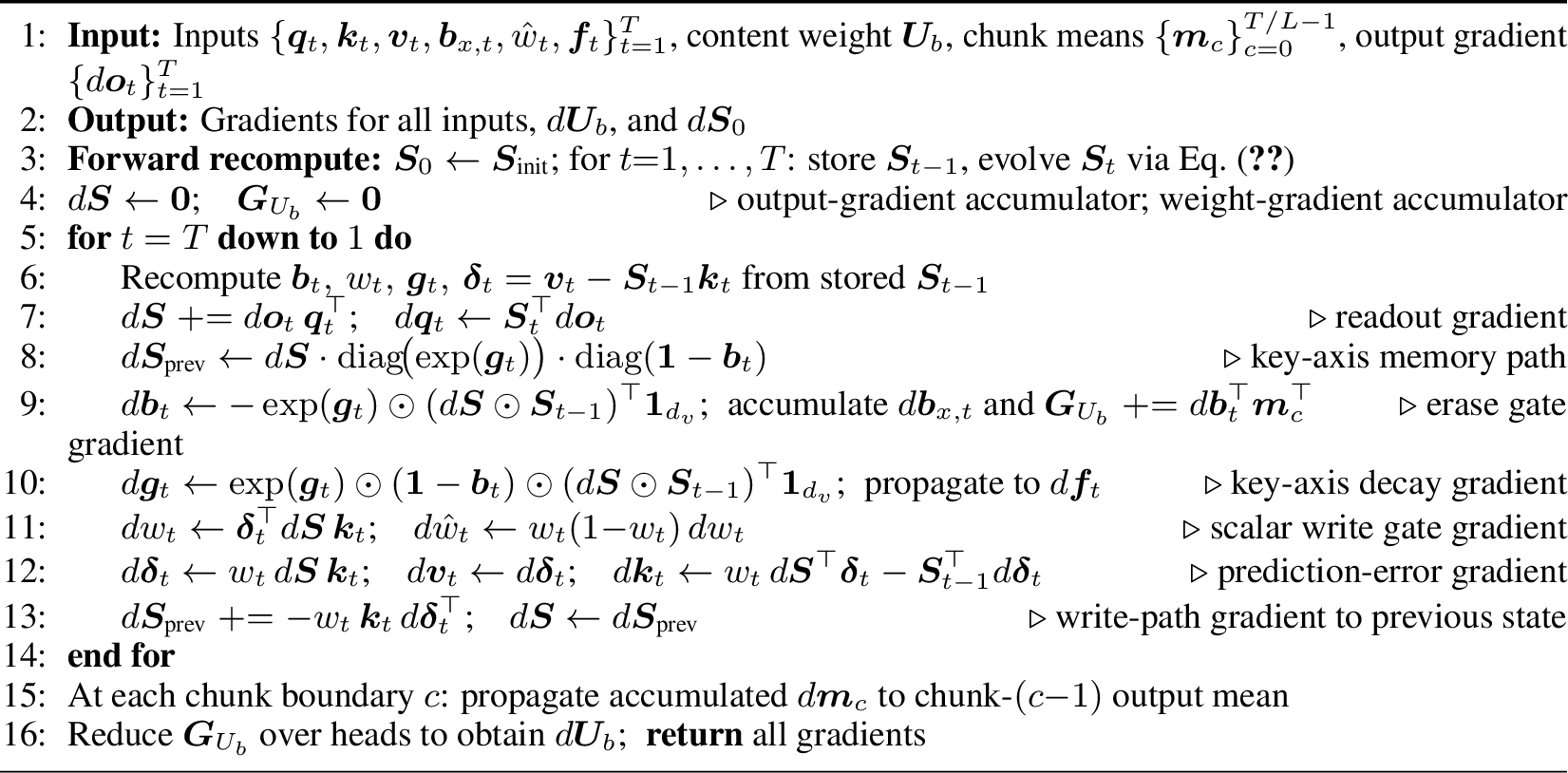
11.1.0.1 Correctness note.
The gradient to the scalar write gate \(w_t\) is \(\boldsymbol{\delta}_t^\top d\boldsymbol{S}\,\boldsymbol{k}_t\) (line 9), whereas the gradient to the prediction error \(\boldsymbol{\delta}_t\) is \(w_t\,d\boldsymbol{S}\,\boldsymbol{k}_t\) (line 10). Conflating these two quantities leaves the gradient of \(w_t\) wrong by order unity while every other gradient remains correct—a failure mode caught only by the per-tensor exactness check of Table 1, which confirms the discrepancy is absent.
12 Training Hyperparameters↩︎
Table 7 reports all hyperparameters used in the \(125\)M (ablation) and \(1.3\)B (main results) training runs. All experiments use the DeepSeek-V3 tokeniser with a \(32\)K vocabulary, AdamW optimiser, and a cosine learning-rate schedule with a linear warmup. For the hybrid configuration, the \(3{:}1\) CARVE:SWA ratio was selected via grid search over \(\{1{:}1, 2{:}1, 3{:}1, 4{:}1\}\) at \(125\)M scale.
| Hyperparameter | 125M | 1.3B |
|---|---|---|
| Hidden dim \(d\) | 768 | 2048 |
| Num heads \(H\) | 12 | 16 |
| Key/value dim \(d_k = d_v\) | 64 | 128 |
| Depth \(D\) | 12 | 24 |
| CARVE:SWA ratio | – | 3:1 |
| Content proj.rank \(r\) | 16 | 32 |
| Chunk size \(L\) | 64 | 128 |
| SWA window \(W\) | – | 1024 |
| MLP width | 2048 | 5632 |
| Sequence length \(T\) | 1024 | 4096 |
| Batch size (tokens) | – | 4M |
| Peak LR | \(3{\times}10^{-4}\) | \(1.5{\times}10^{-4}\) |
| LR schedule | cosine | cosine |
| Warmup steps | 1000 | 10000 |
| AdamW \((\beta_1,\beta_2)\) | \((0.9, 0.95)\) | \((0.9, 0.95)\) |
| Weight decay | 0.1 | 0.1 |
| Gradient clip | 1.0 | 1.0 |
| Training tokens | – | 100B |
| Dataset | – | FineWeb-Edu |
| Vocabulary | 32K | 32K (DeepSeek-V3) |
| Precision | bf16 | bf16 |
| Hardware | 1\(\times\)H100 | Multi-GPU H100 |
13 Comprehensive Architecture Comparison↩︎
Table ¿tbl:tab:comprehensive? places CARVE in the context of eleven representative sequence models across thirteen architectural dimensions. The table distinguishes erase strategy (none, scalar, element-wise matrix, or key-axis rank-1), write strategy, whether gating is content-aware, whether key and value projections are asymmetric, training and inference complexity, and measured throughput on a single H100. The goal is to make the design space legible, not just to rank architectures: the “Content-aware exact recurrent” row illustrates the throughput penalty (\(3.8\times\) slowdown vs.CARVE) paid for an exact per-token content signal, motivating the output-reuse approximation.
3pt max width=
CARVE is the Pareto-efficient operating point: it employs the WY-form chunk solver unmodified, adds content-awareness and scalar write efficiency at near-zero throughput cost (\(-0.4\%\)), and delivers better language-modelling quality (\(-0.18\) WikiText perplexity at \(1.3\)B/\(100\)B tokens) with \(-19\%\) parameters and \(-13\%\) memory.
14 Fast-Weight Programmer Interpretation↩︎
The CARVE state update has an equivalent formulation as a one-step online gradient descent on an associative memory loss, placing it in the tradition of fast-weight programmers [22] and Hebbian linear attention [8]. This section derives that interpretation and shows how the scalar write gate \(w_{h,t}\) functions as a per-head gradient step-size.
The CARVE state update admits an online learning interpretation. Define the decayed state \(\bar\boldsymbol{S}_t = \boldsymbol{S}_{t-1}\boldsymbol{R}_t\), where \(\boldsymbol{R}_t = \operatorname{diag}(\exp(\boldsymbol{g}_t)\odot(\mathbf{1}-\boldsymbol{b}_t))\). Then \(\boldsymbol{S}_t = \bar\boldsymbol{S}_t + w_{h,t}(\boldsymbol{v}_t - \bar\boldsymbol{S}_t\boldsymbol{k}_t)\boldsymbol{k}_t^\top\) is the solution of: \[\boldsymbol{S}_t = \operatorname*{arg\,min}_{\boldsymbol{S}}\; \underbrace{\|\boldsymbol{S} - \bar\boldsymbol{S}_t\|_F^2}_{\text{proximity to decayed state}} - 2w_{h,t}\bigl\langle \boldsymbol{S}\boldsymbol{k}_t,\; \boldsymbol{v}_t - \bar\boldsymbol{S}_t\boldsymbol{k}_t \bigr\rangle.\] The second term applies an associative edit: it writes the delta-rule correction \((\boldsymbol{v}_t - \bar\boldsymbol{S}_t\boldsymbol{k}_t)\) into the association at \(\boldsymbol{k}_t\), scaled by the per-head write gate \(w_{h,t}\). This unifies CARVE with the fast-weight programmer perspective [8], [22], [24].
15 Additional Mathematical Connections↩︎
This section collects a few compact derivations from the broader CARVE draft that complement the main appendix.
15.1 CARVE as Linearised Cross-Attention↩︎
Proposition 14 (CARVE as linearised cross-attention). CARVE’s output computation \(\boldsymbol{y}_t = \boldsymbol{S}_t \boldsymbol{q}_t\) is equivalent to linearised cross-attention [13] in which the past sequence is compressed into \(\boldsymbol{S}_t\) and the softmax kernel is replaced by the identity feature map.
Proof. Standard linearised attention writes \[\boldsymbol{y}_t \approx \sum_{s \le t} (\boldsymbol{q}_t^\top \boldsymbol{k}_s)\boldsymbol{v}_s = \left(\sum_{s \le t} \boldsymbol{v}_s \boldsymbol{k}_s^\top\right)\boldsymbol{q}_t.\] Identifying \(\boldsymbol{S}_t = \sum_{s \le t} \boldsymbol{v}_s \boldsymbol{k}_s^\top\) gives \(\boldsymbol{y}_t = \boldsymbol{S}_t \boldsymbol{q}_t\), which is exactly the linear-attention readout. CARVE generalises this with error-corrective writes and selective forgetting. ◻
15.2 Delta Rule as Online Learning↩︎
Proposition 15 (Delta rule as gradient descent on associative loss). For rank-\(R\) updates, the delta correction \[\boldsymbol{\Delta}_t^{(R)} = \sum_{r=1}^R \bigl(\boldsymbol{v}_t^{(r)} - \boldsymbol{S}_{t-1}\boldsymbol{k}_t^{(r)}\bigr)(\boldsymbol{k}_t^{(r)})^\top\] is the negative gradient of the instantaneous associative loss \[\ell_t(\boldsymbol{S}) = \frac{1}{2}\sum_{r=1}^R \|\boldsymbol{S}\boldsymbol{k}_t^{(r)} - \boldsymbol{v}_t^{(r)}\|_2^2\] evaluated at \(\boldsymbol{S}_{t-1}\).
Proof. Differentiating gives \[\nabla_{\boldsymbol{S}}\ell_t(\boldsymbol{S}) = \sum_{r=1}^R (\boldsymbol{S}\boldsymbol{k}_t^{(r)} - \boldsymbol{v}_t^{(r)})(\boldsymbol{k}_t^{(r)})^\top.\] Substituting \(\boldsymbol{S}= \boldsymbol{S}_{t-1}\) yields \(\nabla_{\boldsymbol{S}}\ell_t(\boldsymbol{S}_{t-1}) = -\boldsymbol{\Delta}_t^{(R)}\). ◻
Theorem 16 (Online regret bound for CARVE-style delta updates). Assume unit-norm keys \(\|\boldsymbol{k}_t^{(r)}\|_2 = 1\) and bounded values \(\|\boldsymbol{v}_t^{(r)}\|_2 \le V\). Then delta-rule updates with step size \(\eta=1\) satisfy \[\sum_{t=1}^T \ell_t(\boldsymbol{S}_{t-1}) - \min_{\boldsymbol{S}}\sum_{t=1}^T \ell_t(\boldsymbol{S}) \le \frac{\|\boldsymbol{S}^\star - \boldsymbol{S}_0\|_F^2}{2} + \frac{TRV^2}{2},\] where \(\boldsymbol{S}^\star = \arg\min_{\boldsymbol{S}}\sum_{t=1}^T \ell_t(\boldsymbol{S})\).
Proof. This is the standard online gradient descent bound for convex losses [33]. By Proposition 15, the CARVE write term is exactly one gradient step on \(\ell_t\). The gradient norm is bounded by \(\|\nabla \ell_t\|_F^2 \le RV^2\), so summing the usual per-step inequality gives the stated result. ◻