Hierarchical Muon: Tiled Newton–Schulz Updates for Efficient Muon Optimization
June 25, 2026
Abstract
Muon-type optimizers construct update directions for dense neural-network weights by applying a finite Newton–Schulz map to momentum-gradient matrices. For an \(H\times W\) matrix, with \(r=\min\{H,W\}\) and \(s=\max\{H,W\}\), \(K\) steps of the full-matrix Newton–Schulz update require \(\mathcal{O}(r^2sK)\) work and couple all rows and columns through repeated Gram matrix products. We introduce Hierarchical Muon (HiMuon), a tiled Newton–Schulz scheme for Muon-type optimization. HiMuon partitions each momentum-gradient matrix into \(T\times T\) tiles, applies the same finite Newton–Schulz map independently to each tile, and reassembles the results. For finite \(T\) below the matrix dimensions, HiMuon defines a local matrix-function map rather than a convergent approximation to the full-matrix update: spectral interactions are preserved within tiles and discarded across tile boundaries. For fixed finite \(T\), the leading Newton–Schulz work decreases to \(\mathcal{O}(HWTK)\), and the computation decomposes into independent small dense matrix operations. This structure enables tile-size-dependent GPU kernels, cross-layer batching, memory-bounded chunking, and runtime tile-size schedules. Experiments on transformer training and controlled matrix-function diagnostics show that HiMuon improves optimizer-step efficiency while keeping training behavior close to full-matrix Muon in the tested regimes. Our implementation is publicly available at https://github.com/tang0389/himuon.
Newton–Schulz iteration, tiled matrix-function updates, polar decomposition, LLM training, batched GPU linear algebra, finite-precision arithmetic
65F30, 90C06, 68T07
1 Introduction↩︎
In transformer models, a large share of the parameter count and arithmetic cost is concentrated in dense projection matrices in the attention and feed-forward sublayers. The gradients of these parameters inherit the same matrix form. Muon-type optimizers exploit this structure by applying a finite Newton–Schulz (NS) iteration to the momentum-gradient matrix associated with each matrix parameter [1]. The output is used as the update direction. This finite-step matrix function acts as a polar-factor surrogate: it drives the singular values of the update direction toward a common scale. Such matrix-function updates have been shown empirically to improve pretraining efficiency across several model scales [2]–[4].
The full-matrix Newton–Schulz map is a major computational component of the Muon optimizer step. For an \(H\times W\) momentum-gradient matrix, let \(r=\min\{H,W\}\) and \(s=\max\{H,W\}\). With the iteration oriented so that the Gram matrix has dimension \(r\), \(K\) Newton–Schulz steps require \[\mathcal{O}(r^2sK) = \mathcal{O}\!\left(HW\min\{H,W\}K\right)\] operations. When \(H\le W\), this becomes \(\mathcal{O}(H^2WK)\). The repeated Gram matrix products also create global spectral coupling: an entry of the update can depend on the entire momentum-gradient matrix. Thus the computational cost of the update and its spectral behavior are linked. Retaining full-matrix spectral coupling gives the standard Muon update, but doing so at every optimizer step requires large dense matrix products. In distributed parameter-sharded training, the full-matrix Newton–Schulz iteration may also require reconstructing matrix shards through additional collective communication inside the optimizer step.
In this paper, we study a tiled formulation in which the extent of this spectral coupling is controlled explicitly by the tile size. Tiling simultaneously reduces the cost of dense matrix products, localizes the Newton–Schulz computation within shard-resident submatrices, and exposes more parallel work to the hardware. Full-matrix Muon represents one extreme, where the Newton–Schulz map is applied to the entire matrix. Coordinatewise methods represent the opposite extreme, where no matrix-level spectral interaction is retained. Between these regimes is a family of local matrix-function updates: the same Newton–Schulz map is applied, but only to submatrices of a prescribed size. The goal is to retain useful local spectral behavior while reducing the cost of the optimizer step and exposing more parallel work to the hardware.
We introduce Hierarchical Muon (HiMuon), a tiled Newton–Schulz method based on this principle. Let \(\Phi_K\) denote the \(K\)-step Newton–Schulz map used in Muon. For a tile size \(T\), HiMuon partitions a momentum-gradient matrix into an \(R\times C\) grid of \(T\times T\) tiles, applies \(\Phi_K\) independently to each tile, and reassembles the tile outputs. For fixed finite \(T\) below the matrix dimensions, this construction does not recover the full-matrix Muon map. It defines a distinct local matrix-function update: spectral interactions are preserved within each tile and removed across tile boundaries. The tile size therefore acts as both a numerical parameter, controlling the amount of retained spectral coupling, and a computational parameter, controlling the cost of the Newton–Schulz computation. For fixed \(T\ll\min\{H,W\}\), the leading Newton–Schulz work scales as \[\mathcal{O}(HWTK).\]
The tiled formulation changes more than the arithmetic count. Once the partition is fixed, all tilewise Newton–Schulz evaluations are independent, so the optimizer step becomes a batched small-matrix linear algebra workload rather than a sequence of large full-matrix operations. HiMuon exploits this structure through tile-size-dependent kernels, cross-layer batching, memory-bounded chunking, and runtime tile-size schedules. The same representation also supports distributed layouts in which each rank performs its tiled Newton–Schulz work locally. In this sense, the numerical locality of the update and the GPU execution strategy are designed together.
The main contributions of this work are summarized as follows.
A tiled Newton–Schulz formulation of Muon. We define HiMuon as a finite-tile matrix-function update for Muon-type optimization. The formulation makes the degree of spectral coupling explicit through the tile size and distinguishes the full-matrix Muon update from local tiled alternatives.
An end-to-end GPU implementation. We develop an implementation that maps the tiled Newton–Schulz workload to batched small dense matrix operations, using tile-size-dependent kernels, cross-layer batching, memory-bounded chunking, and support for distributed parameter layouts.
Empirical characterization across quality, speed, and precision. We evaluate HiMuon at the matrix-function, layer, optimizer-step, and end-to-end training levels. The experiments study real transformer weight shapes, kernel and tile-shape choices, cross-layer batching, finite-precision Newton–Schulz computation, and the resulting training-quality trade-off. We also use an associative-memory benchmark as a structural diagnostic for tile-size selection.
The remainder of the paper is organized as follows. 2 introduces notation, the polar decomposition, the finite Newton–Schulz iteration, and the baseline Muon optimizer. 3 reviews efficient variants of Muon-type optimization and alternative reductions of the Newton–Schulz computation. 4 presents the HiMuon algorithm and its GPU implementation. 5 introduces a capacity-based diagnostic for the tiled map. 6 reports numerical experiments on training quality, computational efficiency, cross-layer batching, and finite-precision behavior. 7 concludes the paper.
2 Preliminaries↩︎
This section fixes the notation and the full-matrix Muon update used as the baseline throughout the paper. We first introduce matrix norms and the tiling operator, then distinguish the exact polar factor from the finite Newton–Schulz map used by Muon, and finally state the optimizer update that HiMuon modifies.
2.1 Notation↩︎
Matrices are denoted by bold uppercase letters, e.g., \(\mathbf{A}\), and \(\mathbf{I}\) denotes an identity matrix of the appropriate dimension. The model parameters are collected in \(\boldsymbol{\theta}\), and the training objective is \(\mathcal{L}(\boldsymbol{\theta})\). Subscript \(t\) denotes the optimizer step. For \(\mathbf{A}\in\mathbb{R}^{H\times W}\), we write \(\left\lVert \mathbf{A} \right\rVert_F\) and \(\left\lVert \mathbf{A} \right\rVert_2\) for the Frobenius and spectral norms.
For a finite tile size \(T\), let \(\mathcal{B}_{T}\) denote the tiling operator. Given \(\mathbf{A}\in\mathbb{R}^{H\times W}\), define \[R=\left\lceil H/T\right\rceil, \qquad C=\left\lceil W/T\right\rceil .\] The operator \(\mathcal{B}_{T}\) pads \(\mathbf{A}\) with zeros, if needed, to an \((RT)\times(CT)\) matrix and partitions the padded matrix into an \(R\times C\) grid of \(T\times T\) tiles: \[\mathcal{B}_{T}(\mathbf{A}) = \{\mathbf{A}_{rc}\}_{r=1,\ldots,R;\,c=1,\ldots,C}, \qquad \mathbf{A}_{rc}\in\mathbb{R}^{T\times T}.\] The inverse operation \(\mathcal{B}_{T}^{-1}\) denotes reassembly of the tiles followed by removal of the padding. We reserve the notation \(T=\infty\) for the no-tiling case, in which the full matrix is processed as a single object rather than padded to a square tile. Rectangular tiles \((T_h,T_w)\) are used only in the tile-shape study of 9; elsewhere \(T_h=T_w=T\).
2.2 Polar Factor and Newton–Schulz Map↩︎
We first recall the row-oriented polar factor. Suppose \(\mathbf{A}\in\mathbb{R}^{H\times W}\) has full row rank and \(H\le W\). Its row polar decomposition is \[\label{eq:polar95decomp} \mathbf{A}= \mathbf{U}\mathbf{P},\tag{1}\] where \(\mathbf{U}\in\mathbb{R}^{H\times W}\) has orthonormal rows, \(\mathbf{U}\mathbf{U}^\top=\mathbf{I}\), and \(\mathbf{P}=(\mathbf{A}^\top\mathbf{A})^{1/2}\) is symmetric positive semidefinite [5], [6]. The factor \(\mathbf{U}=\mathop{\mathrm{polar}}(\mathbf{A})\) is the closest row-orthonormal matrix to \(\mathbf{A}\) in any unitarily invariant norm. When \(\mathbf{A}\) is rank deficient, the polar factor need not be unique. In this paper, \(\mathop{\mathrm{polar}}(\mathbf{A})\) is used only as an exact reference matrix function; the optimizer update itself is defined by the finite Newton–Schulz map below.
Muon uses a quintic Newton–Schulz iteration as a finite polar-factor surrogate. For a nonzero matrix \(\mathbf{A}\in\mathbb{R}^{H\times W}\) with \(H\le W\), set \[\mathbf{X}_0=\frac{\mathbf{A}}{\left\lVert \mathbf{A} \right\rVert_F} .\] The row-oriented recurrence is \[\label{eq:ns95iteration} \mathbf{X}_{k+1} = \bigl( a\mathbf{I} + b\mathbf{X}_k\mathbf{X}_k^\top + c(\mathbf{X}_k\mathbf{X}_k^\top)^2 \bigr)\mathbf{X}_k ,\tag{2}\] with coefficients \[\label{eq:ns95quintic} (a,b,c)=(3.4445,-4.7750,2.0315),\tag{3}\] as in the Muon implementation [1]. Here \(\mathbf{I}\) has dimension \(H\times H\). If \(H>W\), the same recurrence is applied to \(\mathbf{A}^\top\) and the result is transposed back, so the Gram matrix in the iteration always has dimension \(\min\{H,W\}\). For the zero matrix, we set \(\Phi_K(\mathbf{0})=\mathbf{0}\).
We denote the result after \(K\) Newton–Schulz steps by \[\label{eq:phi95k95def} \Phi_K(\mathbf{A}) := \mathbf{X}_K .\tag{4}\] The map \(\Phi_K\) should not be identified with the exact polar factor. It is a finite Newton–Schulz map used to construct the optimizer direction. Although it drives singular values toward a common scale, it is not an exact polar decomposition.
2.3 The Muon Update↩︎
We now state the full-matrix Muon update that HiMuon modifies. Let \(\mathbf{W}_{t-1}\in\mathbb{R}^{H\times W}\) be a two-dimensional parameter matrix at optimizer step \(t\), and let \[\mathbf{G}_t = \nabla_{\mathbf{W}}\mathcal{L}(\boldsymbol{\theta}_{t-1})\] be its gradient. Muon first updates a momentum buffer, \[\label{eq:muon95momentum} \mathbf{M}_t = \beta\mathbf{M}_{t-1}+\mathbf{G}_t ,\tag{5}\] and then forms the Nesterov-type momentum gradient \[\label{eq:muon95lookahead} \widehat{\mathbf{G}}_t = \mathbf{G}_t+\beta\mathbf{M}_t .\tag{6}\] The matrix-valued update direction is obtained by applying the finite Newton–Schulz map to this momentum gradient: \[\label{eq:muon95direction} \mathbf{U}_t = \Phi_K(\widehat{\mathbf{G}}_t).\tag{7}\] With learning rate \(\eta\) and decoupled weight-decay coefficient \(\lambda\), the core parameter update is \[\label{eq:muon95update} \mathbf{W}_t = (1-\eta\lambda)\mathbf{W}_{t-1} - \eta\mathbf{U}_t .\tag{8}\] Equations 7 –8 define the full-matrix baseline. HiMuon keeps the momentum and weight-decay structure of Muon, but replaces the single full-matrix application of \(\Phi_K\) in 7 by tilewise applications of the same finite map.
3 Related Work↩︎
This section places HiMuon in context with prior work on Muon-type optimization and efficient matrix-function updates. We organize the discussion around five themes: update scaling, structured decompositions of the Newton–Schulz computation, alternative reductions of the Muon matrix function, batched GPU execution, and theoretical or diagnostic benchmarks.
3.1 Scaling and normalization in Muon-type optimizers↩︎
Muon-type optimizers apply a finite Newton–Schulz map to momentum-gradient matrices, but their practical behavior also depends on how the resulting update is scaled. Liu et al. [2] identify weight growth and shape-dependent update magnitudes as obstacles to scaling Muon, and address them through decoupled weight decay and a shape-dependent learning-rate scaler. Other variants modify the normalization before or after the Newton–Schulz map. MuonEq [7] equilibrates rows and columns before applying the map; Muon+ [8] and NorMuon [9] normalize the update after the map; RMNP [10] replaces the map by row-wise normalization; and TrasMuon [11] adds feature-wise trust-region clipping. These methods show that Muon-type optimization depends not only on singular-value homogenization, but also on how update magnitudes are balanced across rows, neurons, and parameter shapes.
3.2 Structured decompositions of Newton–Schulz updates↩︎
A closely related line of work reduces the cost of Muon by replacing one global Newton–Schulz update with smaller structured subproblems. GLM-5 [12] applies Muon independently to each attention-head submatrix, while Group Muon [13] treats the head-group size as a tunable hyperparameter; Boreiko et al. [14] study row-wise, column-wise, and square block splitting whose block sizes follow the tensor-parallel degree. MuonBP [15] uses block orthogonalization together with periodic global correction, while DASH [16] demonstrates the efficiency of batched block updates in Shampoo-type methods. TEON [17] takes a different direction by coupling multiple layers through tensorized orthogonalization. These methods decompose matrix-valued update computations using units motivated by model semantics, parallel layouts, correction schemes, or cross-layer tensor structure. HiMuon instead uses fixed two-dimensional intra-matrix tiles whose size is not determined by the sharding layout, making the tile size both a numerical parameter and a GPU execution parameter.
3.3 Alternative reductions of the Muon matrix function↩︎
Other approaches reduce Muon cost by changing the matrix being transformed, the polynomial map, or the matrix-function surrogate. Dion2 [18] orthogonalizes selected rows with error feedback, while Magma [19] uses stochastic masking based on momentum-gradient alignment. Turbo-Muon [20] reduces the number of Newton–Schulz steps; PRISM [21] adapts the polynomial coefficients to the observed spectrum; and IFNSO [22] replaces the iteration by a learned polynomial operator. MUD [23] uses triangular whitening instead of Newton–Schulz, and PolarGrad [24] studies orthogonalized updates from a broader matrix-optimization perspective. This line of work modifies the operator used to approximate or replace the polar-factor surrogate. HiMuon keeps the finite Newton–Schulz map itself unchanged, but changes the domain on which it is applied.
3.4 Batched GPU execution↩︎
Tiled Newton–Schulz computation exposes many independent small dense matrix products. This connects HiMuon to batched small-matrix linear algebra, where grouping independent operations is important for GPU utilization [25]. Related implementation ideas include epilogue fusion, on-chip data reuse, and custom Triton kernels [26], [27]. HiMuon uses these ideas inside the optimizer step through tilewise Newton–Schulz calls, cross-layer batching, memory-bounded chunking, and runtime tile-size reconfiguration.
3.5 Theory and diagnostic benchmarks↩︎
Recent theory has begun to clarify why Muon-type updates can differ from scalar adaptive methods. Kim and Oh [28] analyze finite-step Muon convergence; Su [29] studies singular-value homogenization under curvature models; Du and Su [30] derive an activation-aware Newton-Muon update; and Wen et al. [3] benchmark matrix-based optimizers across model scales. The associative-memory benchmark of Kim et al. [31] provides a controlled setting in which full-matrix Muon and SGD have sharply separated one-step capacity scalings. We use this benchmark in 5 as a diagnostic for whether tilewise Newton–Schulz updates retain the qualitative signal-amplification behavior of full-matrix Muon.
Taken together, these lines of work motivate the design studied in this paper. HiMuon keeps the finite Newton–Schulz map used by Muon, but applies it to fixed-size two-dimensional intra-matrix tiles. This choice makes the tile size a numerical parameter, controlling the amount of retained spectral coupling, and an execution parameter, producing uniform small dense matrix problems for batched GPU kernels. The resulting optimizer combines local matrix-function updates, runtime tile-size scheduling, and cross-layer batched execution. The capacity diagnostic in 5 is then used to assess how this local replacement affects the qualitative behavior of full-matrix Muon.
4 The HiMuon Method↩︎
We now present HiMuon. Starting from the full-matrix Muon update in 7 , HiMuon replaces the single application of \(\Phi_K\) to a momentum-gradient matrix by independent applications of the same finite Newton–Schulz map on fixed-size tiles. The tiled update is then implemented as a batched small-matrix workload on the GPU.
4.1 Tiled Newton–Schulz Map↩︎
Let \(\widehat{\mathbf{G}}\in\mathbb{R}^{H\times W}\) be the lookahead momentum gradient defined in 6 . In full-matrix Muon, the update direction is \(\Phi_K(\widehat{\mathbf{G}})\), where \(\Phi_K\) is the finite Newton–Schulz map defined in 2.2. For a finite tile size \(T\), HiMuon applies this map locally. Using the tiling operator \(\mathcal{B}_{T}\) from 2.1, we write \[\label{eq:tiling95operator} \mathcal{B}_{T}(\widehat{\mathbf{G}}) = \bigl\{\widehat{\mathbf{G}}_{rc}\bigr\}_{r=1,\ldots,R;\,c=1,\ldots,C}, \qquad R=\left\lceil H/T\right\rceil,\quad C=\left\lceil W/T\right\rceil ,\tag{9}\] where zero padding is used when needed and each tile \(\widehat{\mathbf{G}}_{rc}\) has size \(T\times T\). HiMuon applies the same map \(\Phi_K\) independently to each tile and then reassembles the outputs: \[\label{eq:tiled95ns} \Phi_{K,T}(\widehat{\mathbf{G}}) := \mathcal{B}_{T}^{-1} \!\left( \bigl\{\Phi_K(\widehat{\mathbf{G}}_{rc})\bigr\}_{r=1,\ldots,R;\,c=1,\ldots,C} \right).\tag{10}\] The inverse operator removes any padding introduced during tiling. 1 illustrates the construction. The special case \(T=\infty\) denotes the full-matrix branch, \[\label{eq:full95branch} \Phi_{K,\infty}(\widehat{\mathbf{G}}) := \Phi_K(\widehat{\mathbf{G}}) .\tag{11}\]

For finite \(T\) below the matrix dimensions, the tiled map is generally different from the full-matrix Muon map: \[\label{eq:tiled95not95global} \Phi_{K,T}(\widehat{\mathbf{G}}) \neq \Phi_K(\widehat{\mathbf{G}}) .\tag{12}\] This difference is structural: tiling does not commute with either the exact polar factor or the finite Newton–Schulz surrogate. It is a local matrix-function map whose tile size controls the amount of retained spectral coupling. Larger tiles preserve more of the full-matrix interaction, while smaller tiles reduce the cost and expose more independent work.
For square tiles, each tile requires \(\mathcal{O}(T^3K)\) arithmetic, and there are approximately \(HW/T^2\) tiles. Thus, up to lower-order padding effects, the leading Newton–Schulz work is \[\label{eq:tiled95cost} \mathcal{O}(HWTK),\tag{13}\] compared with the full-matrix cost \(\mathcal{O}(HW\min\{H,W\}K)\). The same parameter \(T\) determines both the numerical locality of the update and the size of the dense matrix problems issued to the GPU.
4.2 Update Scaling↩︎
As in Muon, we multiply the Newton–Schulz direction by a shape-dependent RMS-matching factor before applying the parameter update. For a full \(H\times W\) matrix, this factor is \(c\sqrt{\max\{H,W\}}\), since a semi-orthogonal reference direction has entrywise RMS \(1/\sqrt{\max\{H,W\}}\). In the tiled case, the Newton–Schulz map acts on \(T\times T\) blocks, so the corresponding factor is the single tile-size-dependent scalar \[\tau(T)=c\sqrt{T}.\] For the no-tiling branch, we set \(\tau_\ell(\infty)=c\sqrt{\max\{H_\ell,W_\ell\}}\) for \(\mathbf{W}^{(\ell)}\in\mathbb{R}^{H_\ell\times W_\ell}\). The scaled update is therefore \[\label{eq:scaled95update} \mathbf{W}_t^{(\ell)} = (1-\eta\lambda)\mathbf{W}_{t-1}^{(\ell)} - \eta\,\tau_\ell(T_t)\, \Phi_{K,T_t}(\widehat{\mathbf{G}}_t^{(\ell)}),\tag{14}\] where \[\tau_\ell(T_t) = \begin{cases} c\sqrt{\max\{H_\ell,W_\ell\}}, & T_t\ge\max\{H_\ell,W_\ell\},\\ c\sqrt{T_t}, & T_t<\max\{H_\ell,W_\ell\} . \end{cases}\] This scaling is a global scalar for each matrix update; it introduces no tilewise adaptation and leaves the learning rate, momentum, and weight decay unchanged from the Muon baseline.
4.3 Complete Algorithm↩︎
2 summarizes the HiMuon update. The index \(\ell\in\mathcal{E}\) enumerates the two-dimensional parameter matrices to which Muon-type updates are applied, with \(\mathbf{W}^{(\ell)}\in\mathbb{R}^{H_\ell\times W_\ell}\). The value \(T_t\) denotes the tile size used at optimizer step \(t\); the special value \(T_t=\infty\) selects the full-matrix branch.
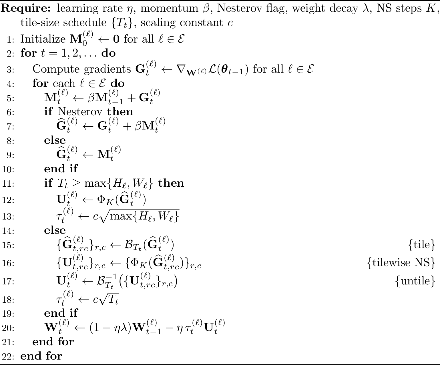
The branch \(T_t\ge\max\{H_\ell,W_\ell\}\), for example \(T_t=\infty\), denotes the full-matrix Muon update. Smaller tile sizes are interpreted through the padding-and-tiling operator \(\mathcal{B}_{T_t}\). For square finite tiles, \(\tau_t^{(\ell)}=c\sqrt{T_t}\) is a single scalar shared by all tiles in the matrix; it introduces no tilewise adaptation. Rectangular tiles use \(\tau_t^{(\ell)}=c\sqrt{\max\{T_h,T_w\}}\) in the tile-shape experiments.
4.4 GPU Implementation↩︎
The mathematical definition of HiMuon creates many independent Newton–Schulz problems, one for each tile. This independence is useful only if the implementation can execute the tilewise computations without introducing new overheads that offset the arithmetic reduction. A naive implementation would allocate a fresh tile tensor and launch many small Newton–Schulz computations every step, writing intermediate matrices to high-bandwidth memory (HBM) between the \(K\) Newton–Schulz steps. These costs can dominate when the tile size is small.
The implementation contribution is therefore an optimizer-level execution plan for the tiled Newton–Schulz map. The plan has three goals: avoid unnecessary data movement, aggregate small independent tile computations into large GPU batches, and allow the tile size to change during training without resetting optimizer state. These choices do not change the mathematical update in 2; they determine how the independent evaluations of \(\Phi_K\) are scheduled on the GPU.
4.4.1 Tile-size-dependent Newton–Schulz kernels↩︎
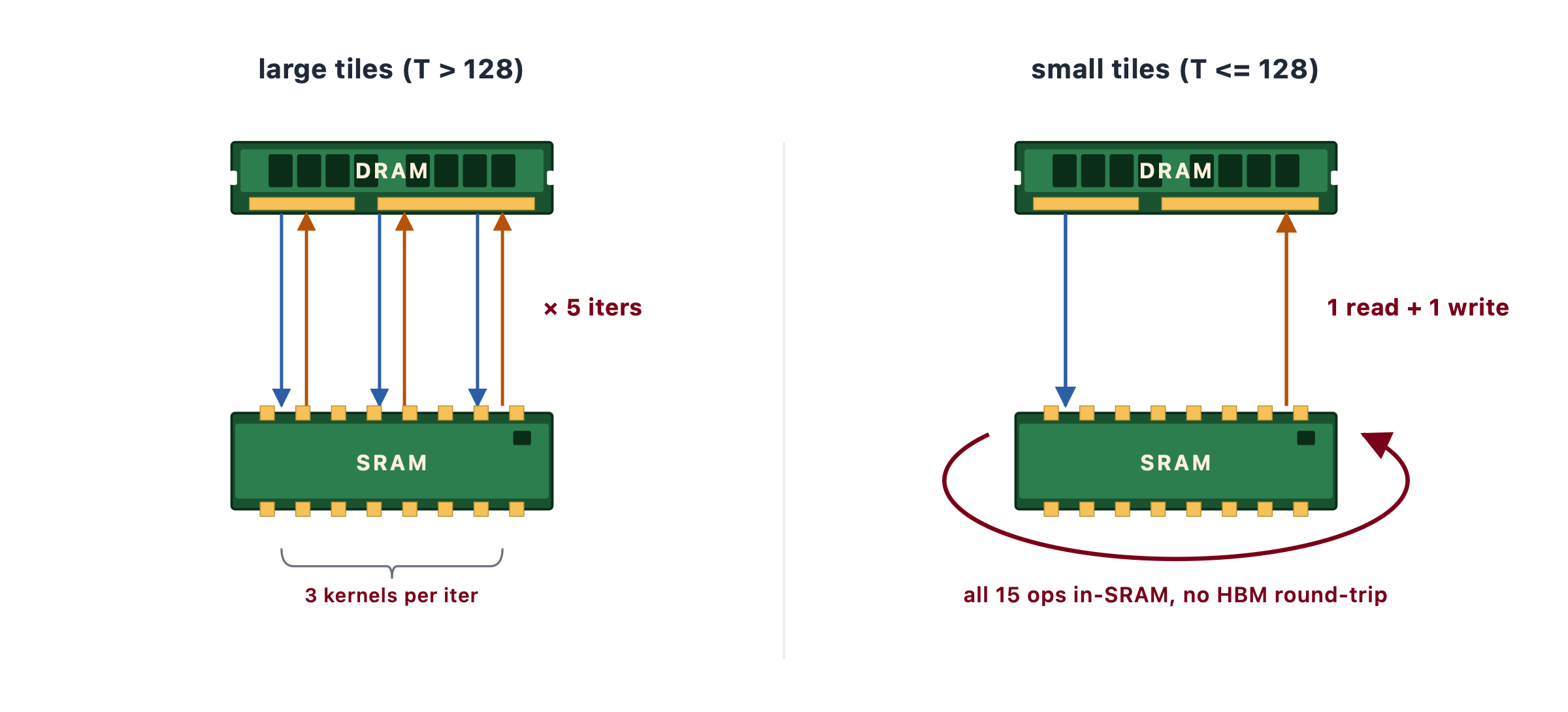
The best kernel strategy depends on the tile size. For larger tiles, each Newton–Schulz step contains enough arithmetic to amortize kernel launches, and HiMuon uses a multi-kernel Triton [26] path. In this path, matrix products and the polynomial update in the Newton–Schulz recurrence are fused where possible before intermediate results are written back to HBM.
For smaller tiles, the arithmetic per tile is lower and repeated memory traffic becomes the main bottleneck. In this regime, the tile working set fits in on-chip static random-access memory (SRAM). HiMuon therefore uses an SRAM-resident kernel that keeps all \(K\) Newton–Schulz iterations inside a single kernel, avoiding intermediate HBM round trips through the iteration loop. The threshold between the two paths is hardware dependent; in our implementation, the SRAM-resident path is used for tiles up to \(T=128\).
3 summarizes this tile-size-dependent dispatch rule. These kernel choices do not change the arithmetic complexity \(\mathcal{O}(HWTK)\); their purpose is to make the reduced arithmetic cost visible in wall-clock time by reducing memory traffic and kernel-launch overhead.
4.4.2 Cross-layer batching↩︎
Tilewise Newton–Schulz evaluations are independent not only within a single matrix, but also across different parameter matrices. This is important in transformer models, where each layer contains several Muon-eligible matrices and each matrix may contain only a moderate number of tiles. Launching one Newton–Schulz computation per matrix can underutilize the GPU because each launch may expose too little work.
HiMuon thus groups compatible tiles across layers into larger batched Newton–Schulz calls. Tiles are compatible when they have the same tile shape, dtype, and kernel path. The batched call computes the same tilewise outputs as processing each matrix separately; only the execution order changes. Momentum buffers, parameter tensors, and weight decay remain indexed by the original parameter \(\ell\), so cross-layer batching is an implementation strategy rather than a change to the optimizer update.
For large models, a single global batch of all compatible tiles may exceed the available memory budget. HiMuon handles this with memory-bounded chunking: the batched tile set is split into the fewest chunks whose input, intermediate workspace, and output fit within a prescribed memory budget. Since the Newton–Schulz evaluations are independent across tiles, chunking is mathematically equivalent to processing the full batch at once. It only bounds temporary memory usage.
In single-GPU and Distributed Data Parallel (DDP) runs, the batched tiles are assembled during each optimizer step into reusable batched buffers whose storage is cached across steps. Under the bank-sharded Fully Sharded Data Parallel (FSDP) layout used in our experiments, same-shape matrices are stored along a leading batch axis, so each rank owns a subset of complete matrices in its local shard. The tiled Newton–Schulz computation is therefore rank-local and does not require an optimizer-internal all-gather.
4.4.3 Runtime tile-size reconfiguration↩︎
The tile size is exposed as a runtime parameter rather than being fixed at optimizer construction. A reconfigure() routine updates the tile-dependent execution plan when \(T_t\) changes. This plan includes
tile indexing metadata, batching buckets, chunking decisions, kernel-path selection, and graph-capture state when applicable. The optimizer state itself, including the momentum buffers, is independent of the tile size and is preserved across
reconfiguration.
We treat \(T_t=\infty\) as the full-matrix branch, in which \(\Phi_K\) is applied to the original matrix. Finite tile sizes are interpreted through the padded tiling operator \(\mathcal{B}_{T_t}\), where zero padding only aligns the matrix boundaries with the tile grid: padded rows and columns remain identically zero throughout the iteration 2 and do not affect the Frobenius normalization of the tile. Tiling is therefore meaningful only when \(T_t<\max\{H_\ell,W_\ell\}\). When \(T_t\ge\max\{H_\ell,W_\ell\}\), the partition reduces to a single tile (\(R=C=1\)) and the tiled map coincides with the full-matrix map, \(\Phi_{K,T_t}(\widehat{\mathbf{G}}_t^{(\ell)}) =\Phi_K(\widehat{\mathbf{G}}_t^{(\ell)})\); this case is therefore identified with the full-matrix branch, including its scaling factor \(c\sqrt{\max\{H_\ell,W_\ell\}}\).
In the end-to-end experiments of 6.2, we use a full-to-local schedule, \[T_t = \begin{cases} \infty, & t < t_1,\\ 512, & t_1 \le t < t_2,\\ 128, & t \ge t_2 . \end{cases}\] The initial full-matrix phase preserves global spectral coupling during the earliest optimization steps, when gradient statistics and dominant directions are least settled. The optimizer then switches to lower-cost tiled maps for the remainder of training. The DDP experiments use \((t_1,t_2)=(100,500)\), while the FSDP experiment uses \((t_1,t_2)=(200,500)\). These breakpoints are fixed empirical choices in our experiments. The capacity diagnostic in 5 motivates the full-to-local form of the schedule qualitatively, but does not determine the switch times.
5 Capacity Diagnostic↩︎
Many-step transformer training entangles the effect of the update map with learning-rate schedules, changing gradient statistics, stochasticity, and architecture-specific dynamics. To isolate the effect of replacing a full-matrix Newton–Schulz map by a tiled one, we use the one-step linear associative-memory benchmark of Kim et al. [31]. This benchmark is useful because full-matrix Muon and SGD have sharply separated capacity scalings, so the signal-amplification behavior of matrix-function updates can be observed directly. We use the benchmark as an empirical diagnostic for how the tiled map \(\Phi_{K,T}\) changes this behavior as the tile size varies.
5.1 Linear Associative-Memory Benchmark↩︎
We first recall the benchmark. The task consists of \(N\) key–value pairs \((v_i,u_i)\), where \[v_i,u_i \sim \mathcal{N}(0,d^{-1}\mathbf{I}_d).\] The associations are stored in a matrix \(\mathbf{W}\in\mathbb{R}^{d\times d}\). Given an input key \(v_i\), the model assigns logits \[u_j^{\!\top}\mathbf{W}v_i,\qquad j=1,\ldots,N,\] and is trained with cross-entropy loss to predict the matching value index \(i\). The \(i\)th training example is sampled with probability \(p_i\propto i^{-\alpha}\). Starting from \(\mathbf{W}_0=0\), one optimizer update using a minibatch of size \(B\) produces \(\mathbf{W}_1\). An item \(k\) is counted as recovered if \[\arg\max_j u_j^{\!\top}\mathbf{W}_1 v_k = k .\] The one-step storage capacity is the number of recovered items.
The benchmark separates scalar gradient updates from spectral matrix-function updates through their capacity scalings. Under the assumptions of Kim et al. [31], with \(\alpha>1\) and appropriate scaling of the stabilized polar map, the full-matrix Muon update has one-step capacity \[\label{eq:kim95muon95capacity} \widetilde{\Theta} \!\left( \min\{d^{1+1/(2\alpha)},\,B^{1/\alpha}\} \right),\tag{15}\] where \(B\) is the minibatch size. Under the same data model, SGD has capacity \[\label{eq:kim95sgd95capacity} \widetilde{\Theta} \!\left( \min\{d^{1/(2\alpha)},\,B^{1/\alpha}\} \right).\tag{16}\] Thus, in the dimension-limited regime, the Muon capacity term is larger than the SGD term by a factor of \(d\). The shared term \(B^{1/\alpha}\) is a finite-sample ceiling: items absent from the minibatch provide no direct training signal in the one-step gradient.
A useful interpretation of 15 is bulk singular-value amplification. At initialization, the one-step gradient contains strong directions associated with high-frequency sampled items and a bulk of weaker directions associated with lower-frequency items. A stabilized polar-type update amplifies this bulk more uniformly than a scalar gradient update, enabling recovery of weaker associations. Since HiMuon applies the finite Newton–Schulz map only within tiles, the experiments below test how much of this full-matrix amplification behavior remains after tilewise processing and reassembly.
5.2 Tile-Size Capacity Diagnostic↩︎
The capacity scalings in 15 and 16 are stated for global update maps. HiMuon replaces the full map \(\Phi_K(\cdot)\) by the tiled map \(\Phi_{K,T}(\cdot)\). Each tile can amplify only the singular directions present in its own submatrix, while singular directions whose support spans several tiles are not treated coherently by a single Newton–Schulz map. This suggests a tile-size heuristic: larger tiles should better preserve full-matrix behavior because each tile contains a richer local spectrum, whereas smaller tiles reduce cost but may weaken the reassembled signal amplification. We therefore evaluate two one-step diagnostics: aggregate capacity scaling with dimension and top-\(k\) recovery over the sampled item support.
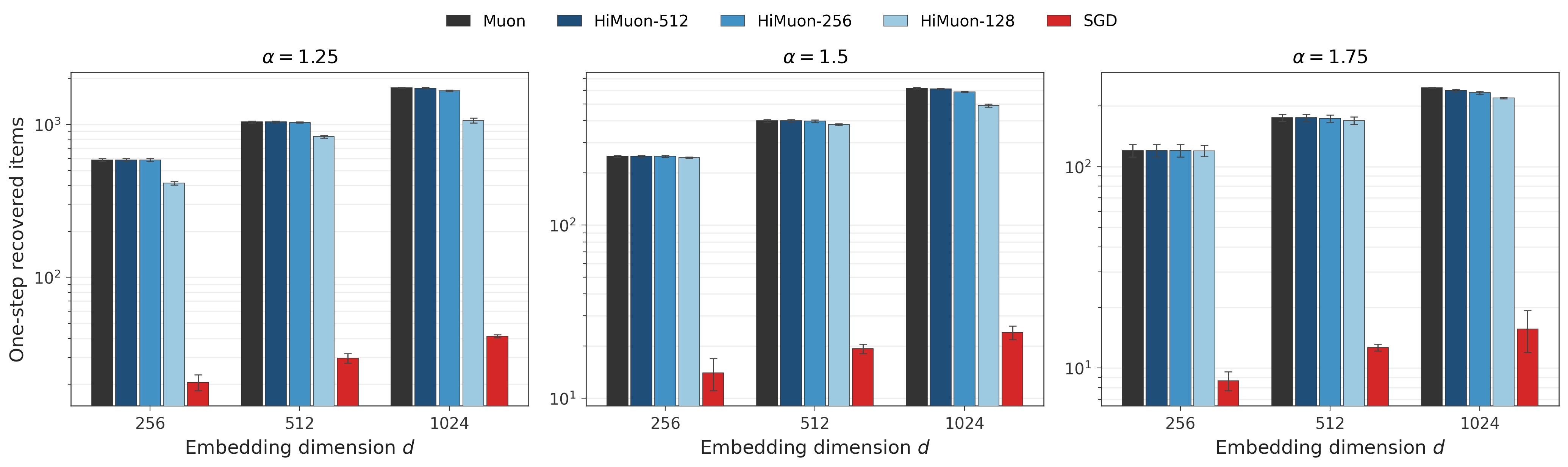
4 reports one-step capacity for SGD, full-matrix Muon, and HiMuon with \(T\in\{128,256,512\}\) across \(\alpha\in\{1.25,1.5,1.75\}\), all within the \(\alpha>1\) regime of 15 . We use \(d\in\{256,512,1024\}\), \(B/d=10\), \(N=10^5\), and three random seeds. Across the tested values of \((d,\alpha)\), the same qualitative ordering is observed: \[\text{Muon}\approx \text{HiMuon-}512 > \text{HiMuon-}256 > \text{HiMuon-}128 \gg \text{SGD}.\] At \(d=1024\), HiMuon-\(512\) is within \(3\%\) of full-matrix Muon across all three values of \(\alpha\), and HiMuon-\(256\) is within \(6\%\). HiMuon-\(128\) trails full-matrix Muon by \(11\%\)–\(39\%\), but remains well above SGD in every panel. The Muon/SGD gap also grows with \(d\), consistent with the dimension-dependent separation predicted by 15 and 16 .
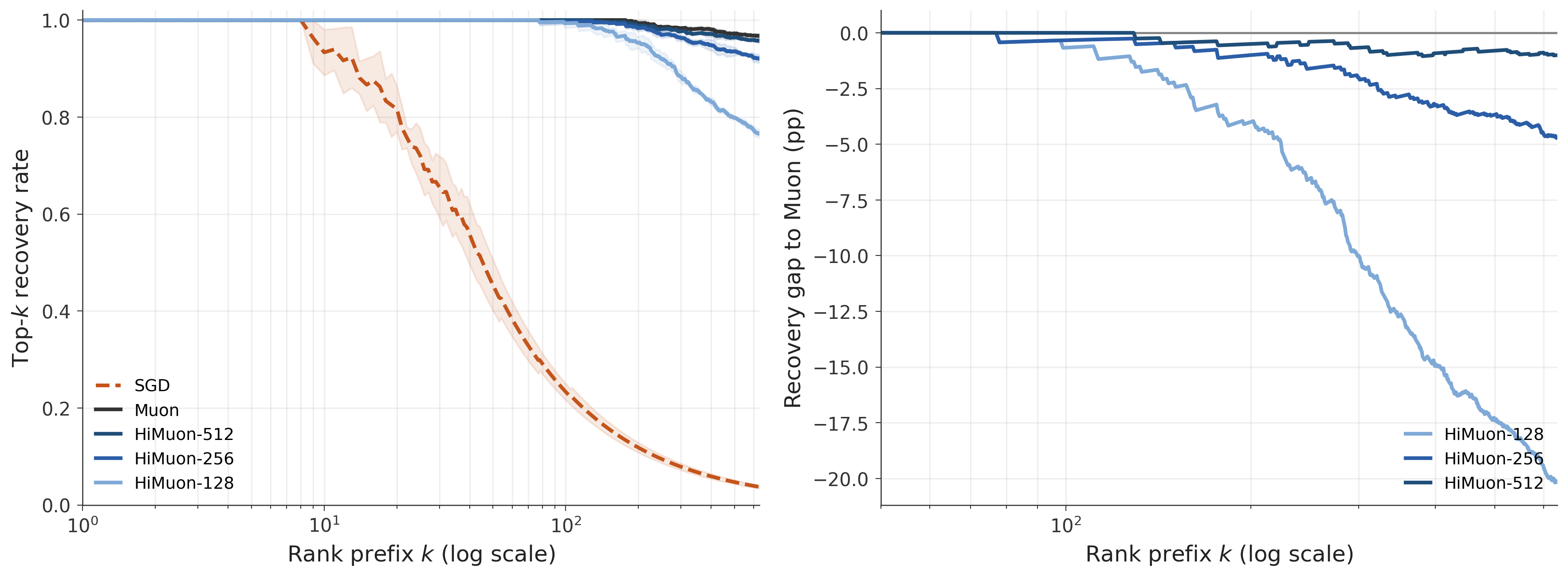
5 examines which sampled items are recovered at \(d=1024\), \(\alpha=1.5\), and \(B/d=10\). We restrict this evaluation to the unique sampled support \(\mathcal{S}\) in the minibatch. This avoids mixing update-map quality with finite-sample coverage, since items outside \(\mathcal{S}\) do not contribute directly to the one-step gradient. Across seeds, \(|\mathcal{S}|\) averages \(639\). We sort sampled items by decreasing population frequency and report top-\(k\) recovery up to the common cutoff \(k_{\max}=632\).
The head of the sampled distribution is insensitive to tile size. Through \(k\approx128\), full-matrix Muon and all HiMuon variants recover nearly all sampled top-\(k\) items, whereas SGD drops much earlier. Tile size matters more deeper in the sampled support, where recovery depends on amplifying weaker directions. At \(k=k_{\max}\), HiMuon-\(128\) trails full-matrix Muon by about \(20\) percentage points, HiMuon-\(256\) by about \(5\) percentage points, and HiMuon-\(512\) by about \(1\) percentage point. This rank-dependent pattern supports the interpretation that high-frequency sampled items are robust to tiling, while recovery of weaker sampled items depends more strongly on the amount of retained spectral coupling.
These diagnostics suggest that the importance of tile size depends on which capacity limit is active. If the finite-sample term \(B^{1/\alpha}\) is the bottleneck, recovery is limited mainly by minibatch coverage, and smaller tiles may be sufficient. If the dimension-dependent Muon term in 15 is the bottleneck, the update map matters more, and larger tiles are needed to better preserve full-matrix spectral behavior. In our experiments, \(T=512\) is closest to full-matrix Muon, \(T=256\) retains much of the gain at lower cost, and \(T=128\) shows visible capacity loss.
The diagnostic also gives a qualitative rationale for the runtime tile-size schedule in 4.4.3. Because the benchmark isolates a one-step update from \(\mathbf{W}_0=0\), it is most analogous to the earliest stage of training, where global spectral coupling is most directly exposed. This motivates using a full-matrix warm start before switching to finite tiles, and using larger tiles before smaller ones in a full-to-local schedule. The benchmark does not determine the switch times or the final tile size; those choices are fixed empirical hyperparameters in the end-to-end experiments.
6 Numerical Experiments↩︎
We evaluate HiMuon along four axes: end-to-end training behavior, matrix-function runtime on transformer layer shapes, optimizer-step speed under cross-layer batching, and robustness to low-precision Newton–Schulz computation. Unless otherwise stated, the baseline is full-matrix Muon [2], and HiMuon uses the same learning rate as the corresponding Muon run. This isolates the effect of replacing the full-matrix Newton–Schulz map by the tiled map.
6.1 Experimental Setup↩︎
Models and data. End-to-end training experiments use Qwen3-0.6B, Qwen3-1.7B, and Qwen3-4B transformer language models [32]. The two smaller models are trained with Distributed Data Parallel (DDP), while the 4B model is trained with Fully Sharded Data Parallel (FSDP). Layer-level performance studies use the same model family to probe the larger-matrix regime. Training uses the FineWeb dataset [33] in streaming mode with sequence length \(1024\), drawing from its official sample-10BT subset (\({\sim}10\)B tokens). Held-out evaluation uses FineWeb’s CC-MAIN-2024-51 configuration, a Common Crawl snapshot disjoint from the training sample.
Optimizer settings. Unless otherwise stated, HiMuon uses momentum \(\beta=0.95\) and \(K=5\) Newton–Schulz steps, following the default setting of Muon [2], with the update scaling of 4.2 and \(c=0.2\). The end-to-end runs use the runtime tile-size schedule described in 4.4.3: an initial full-matrix phase, followed by \(T=512\), then \(T=128\). The DDP runs switch at steps \(100\) and \(500\), while the FSDP run switches at steps \(200\) and \(500\). Isolated matrix-function, kernel, and optimizer-step studies use a fixed tile size, stated with each experiment.
The learning rate is selected by grid search for full-matrix Muon, and HiMuon reuses the same value. The DDP runs use a cosine learning-rate schedule with a \(100\)-step linear warmup, decaying to zero. The FSDP run uses a warmup-stable-decay (WSD) schedule with the same \(100\)-step warmup and a final \(400\)-step decay to \(0.1\times\) the peak learning rate.
Hardware and timing protocol. End-to-end training runs use \(4\times\) NVIDIA A40 GPUs: Qwen3-0.6B and Qwen3-1.7B in DDP, and Qwen3-4B in FSDP. Matrix-function, kernel, and optimizer-step performance
studies run on a single NVIDIA A40 GPU unless otherwise stated. Latencies are measured with CUDA events after a warmup phase, and we report medians with interquartile ranges over \(30\)–\(50\) timed repetitions. Layer-level speedups are measured in paired trials: the baseline and test configuration are run back-to-back, and the per-trial ratio is taken. Aggregate step-time and kernel speedups are reported as
ratios of the corresponding medians. Peak memory is the maximum allocated memory (torch.cuda.max_memory_allocated) recorded over a short run of optimizer steps after warmup. All experiments use PyTorch 2.6.0 with CUDA 12.4; for details, please
refer to our code repository.
Numerical precision. All training and performance experiments use bf16 mixed-precision computation, matching the default Muon implementation. The precision studies in [sec:precision_recovery,sec:precision_descent] vary the precision used inside the Newton–Schulz inner GEMMs as described there.
Code availability. The implementation and the scripts for all experiments in this section are available at https://github.com/tang0389/himuon.
6.2 Training Quality↩︎
We first evaluate the effect of the tiled update on end-to-end pretraining. HiMuon replaces one global Newton–Schulz map by many local maps, so the goal is to test whether the wall-clock reduction is accompanied by a visible loss penalty in short training runs. We report next-token cross-entropy on both the training stream and a held-out validation split disjoint from the training data.
Each model is trained for \(1000\) steps on the FineWeb sample-10BT, comparing HiMuon against full-matrix Muon at the same learning rate and a single fixed seed. Qwen3-0.6B and Qwen3-1.7B run in \(4\times\)A40 DDP with an effective batch of \(64\) length-\(1024\) sequences (\(31.3\)M non-padding tokens), using \(\eta=0.02\) and \(\eta=0.01\), respectively. Qwen3-4B runs in \(4\times\)A40 FSDP with an effective batch of \(32\) length-\(512\) sequences and \(\eta=0.005\). The HiMuon schedule starts with the full-matrix branch, so HiMuon and Muon share the same update early in training and differ only after the tile-size switches.
1 reports the training loss at selected steps, smoothed by a trailing mean over the preceding \(50\) steps to reduce minibatch noise. Across checkpoints, the HiMuon–Muon differences are small relative to the loss scale; the tiled run is sometimes lower and sometimes higher.
| Step | |||||||
|---|---|---|---|---|---|---|---|
| 3-8 Model | Optimizer | \(100\) | \(200\) | \(300\) | \(500\) | \(700\) | \(1000\) |
| 0.6B | Muon | \(3.220\) | \(2.913\) | \(2.744\) | \(2.521\) | \(2.338\) | \(2.236\) |
| HiMuon | \(3.183\) | \(2.901\) | \(2.723\) | \(2.493\) | \(2.281\) | \(2.162\) | |
| 1.7B | Muon | \(3.169\) | \(2.909\) | \(2.746\) | \(2.507\) | \(2.305\) | \(2.189\) |
| HiMuon | \(3.162\) | \(2.914\) | \(2.736\) | \(2.495\) | \(2.277\) | \(2.142\) | |
| 4B | Muon | \(4.838\) | \(4.590\) | \(4.082\) | \(3.701\) | \(3.698\) | \(3.719\) |
| HiMuon | \(4.836\) | \(4.583\) | \(4.103\) | \(3.721\) | \(3.717\) | \(3.733\) | |
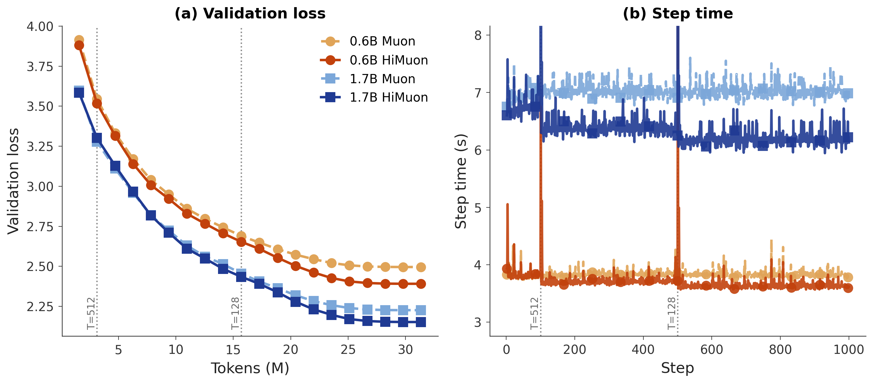
DDP. 6 plots validation loss against tokens processed and per-step wall time for the two DDP models. HiMuon tracks full-matrix Muon through the initial full-matrix phase and then settles to a lower step time after the tile-size switches. In these single-seed runs, the validation losses remain close to, and in these cases below, the corresponding Muon curves.
For Qwen3-0.6B, the step time decreases from \(3.80\) s in the full-matrix phase to \(3.70\) s after the first switch and \(3.62\) s after the second switch, a \(4.7\%\) per-step reduction. Total wall time changes from \(3959\) s to \(3822\) s, a \(3.5\%\) reduction. The final training loss is lower for HiMuon by \(\Delta=-0.074\) at step \(1000\), and the final validation loss is \(2.391\) versus \(2.496\) for Muon.
For Qwen3-1.7B, the larger matrices make the tiled Newton–Schulz computation more beneficial. Step time decreases from \(6.72\) s to \(6.36\) s and then \(6.16\) s, an \(8.3\%\) per-step reduction. Total wall time changes from \(7157\) s to \(6610\) s, a \(7.6\%\) reduction. The final training-loss difference is \(\Delta=-0.047\), and the final validation loss is \(2.152\) for HiMuon versus \(2.226\) for Muon. The brief upward spikes in step time coincide with tile-size switches, where the kernels and cross-layer batching plan are rebuilt; this overhead is amortized over subsequent steps.
FSDP. The Qwen3-4B model is too large for the DDP setup on \(4\times\)A40 and is therefore run under FSDP. Because the Muon baseline in this setting is an FSDP adaptation rather than the implementation used in the DDP runs, we treat the 4B experiment as a quality and scaling check rather than a direct timed comparison. HiMuon’s training loss stays within a few hundredths of full-matrix Muon in 1; the final validation losses are \(3.629\) for HiMuon and \(3.613\) for Muon. HiMuon’s step time decreases as the schedule shrinks the tiles, from \(17.55\) s to \(17.32\) s and then \(17.18\) s after the switches at steps \(200\) and \(500\). End-to-end throughput tuning under FSDP is left to future work.
Overall, the tiled update gives lower wall-clock time in the DDP runs while keeping training and validation losses close to full-matrix Muon in these single-seed experiments. The reported wall-clock reductions should be interpreted as short-run measurements: in these \(1000\)-step runs, the initial full-matrix phase and schedule-switch overheads form a larger fraction of total time than they would in longer pretraining runs.
6.3 Matrix-Function Performance↩︎
We next study the tiled Newton–Schulz map in isolation, separated from the full training loop. This isolates the matrix-function computation from the forward pass, backward pass, communication, and data movement that also contribute to end-to-end training time. The experiments in this subsection measure speedup on real Qwen3 layer shapes, compare kernel strategies, and examine the speed–quality trade-off across tile shapes.
Speedup on real transformer layer shapes. We first measure the isolated tiled/full-matrix Newton–Schulz speedup on actual Qwen3 weight matrices. For each Qwen3 model, we extract the seven Muon-eligible matrices from Block 0:
q_proj, k_proj, v_proj, o_proj, gate_proj, up_proj, and down_proj; their shapes are listed in 2. For each shape, we apply the
full-matrix map \(\Phi_K\) and the tiled map \(\Phi_{K,T}\) with \(T=512\) and \(K=5\) to a single random bf16 Gaussian
matrix of that shape. We report the paired speedup \(t_{\mathrm{full}}/t_{\mathrm{tile}}\) as the median over \(30\) timed repetitions after \(3\) warmup
iterations.
| Model | q_proj | k_proj | v_proj | o_proj | gate_proj | up_proj | down_proj |
|---|---|---|---|---|---|---|---|
| 0.6B | \(2048\times1024\) | \(1024\times1024\) | \(1024\times1024\) | \(1024\times2048\) | \(3072\times1024\) | \(3072\times1024\) | \(1024\times3072\) |
| 1.7B | \(2048\times2048\) | \(1024\times2048\) | \(1024\times2048\) | \(2048\times2048\) | \(6144\times2048\) | \(6144\times2048\) | \(2048\times6144\) |
| 4B | \(4096\times2560\) | \(1024\times2560\) | \(1024\times2560\) | \(2560\times4096\) | \(9728\times2560\) | \(9728\times2560\) | \(2560\times9728\) |
4pt
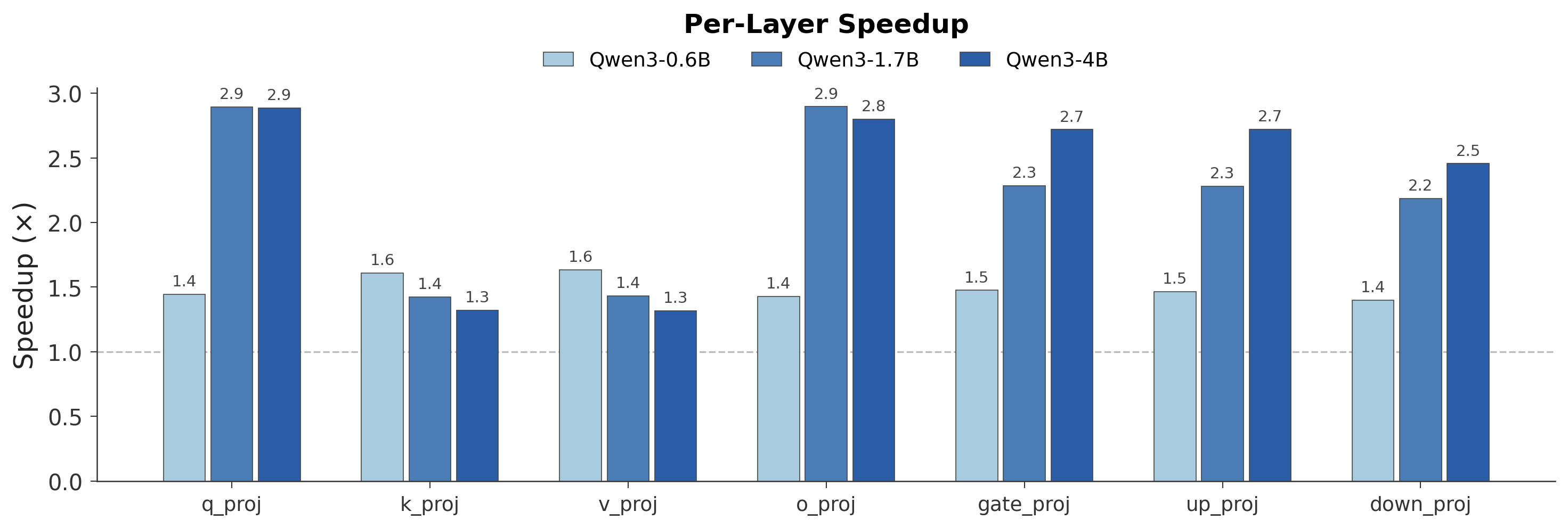
7 shows that the measured per-layer speedups at \(T=512\) range from \(1.4\)–\(1.6\times\) for Qwen3-0.6B, \(1.4\)–\(2.9\times\) for Qwen3-1.7B, and \(1.3\)–\(2.9\times\) for Qwen3-4B. The largest gains occur on the attention projections
q_proj and o_proj and on the wide MLP projections gate_proj, up_proj, and down_proj. In contrast, k_proj and v_proj show smaller gains. Qwen3 uses grouped-query
attention, which reduces the output dimension of these two projections relative to the hidden size; the full-matrix Newton–Schulz work on these narrower matrices is already smaller, so tiling has less work to reduce. Across the remaining projections, the
measurements show that the \(\mathcal{O}(HWTK)\) cost model translates into practical speedups on real transformer weight matrices, with larger gains when \(H\) and \(W\) are large relative to \(T\).
Kernel strategy. The tiled map changes the performance regime of Newton–Schulz. At small tile sizes, the arithmetic work per tile is low, and repeated memory traffic can dominate. Without fusion, each Newton–Schulz iteration writes intermediate matrices to HBM and reads them back. Small tiles are also the regime in which the full \(K\)-step computation can fit in on-chip SRAM, enabling a single SRAM-resident kernel.
We study this regime at \(T=128\), comparing four implementations: a PyTorch eager loop, torch.compile, a three-kernel Triton implementation with epilogue fusion, and an SRAM-resident kernel that keeps all
\(K=5\) Newton–Schulz iterations on chip. Each implementation processes a batch of random bf16 Gaussian \(T\times T\) tiles. We sweep the tile batch size \(B_{\mathrm{tile}}\) and report the median over \(50\) timed repetitions after \(10\) warmup iterations, with speedup measured relative to the eager loop.
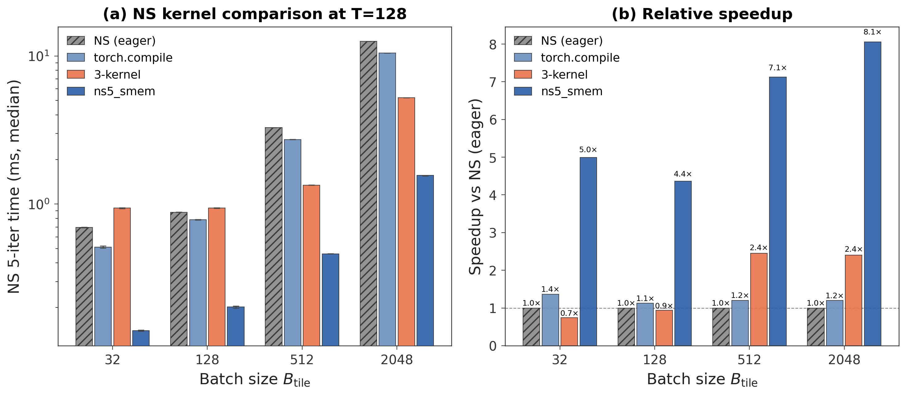
8 shows that the SRAM-resident path gives the largest improvement for \(T=128\), achieving roughly \(4\)–\(8\times\) speedup over eager execution, with the largest gain at \(B_{\mathrm{tile}}=2048\). The three-kernel epilogue-fusion path is useful only at larger batch sizes, where its launch overhead
is amortized. torch.compile gives a smaller but consistent improvement, reflecting partial reduction of launch overhead without fusing the full Newton–Schulz iteration loop.
Tile shape. The tile shape affects both execution and optimization behavior because it defines the local matrix to which \(\Phi_K\) is applied. We compare rectangular tile shapes using two measurements: isolated kernel speed and final training loss for Llama-220M, a small non-Qwen model for inexpensive tile-shape sweeping, trained with HiMuon for \(300\) steps.
For the kernel-speed panel of 9, we sweep tile shapes \((T_h,T_w)\) drawn from \(\{16,32,64,128,256,512,1024,2048\}\), keeping only shapes that fit the A40 SRAM budget. The tile batch size is chosen so that the working set \(B_{\mathrm{tile}}T_hT_w\) is constant across shapes. The reported speedup is the fused NS5 kernel over the three-kernel path. For the training-quality panel, we train Llama-220M on FineWeb sample-10BT for \(300\) steps at batch size \(8\), sequence length \(1024\), and \(\eta=0.02\), using a \(20\)-step linear warmup followed by a \(60\)-step cosine decay to a \(0.1\) learning-rate floor. The experiment uses a single fixed seed and replays the same preloaded batch sequence for every tile shape; the reported loss is the mean over the final \(100\) steps.
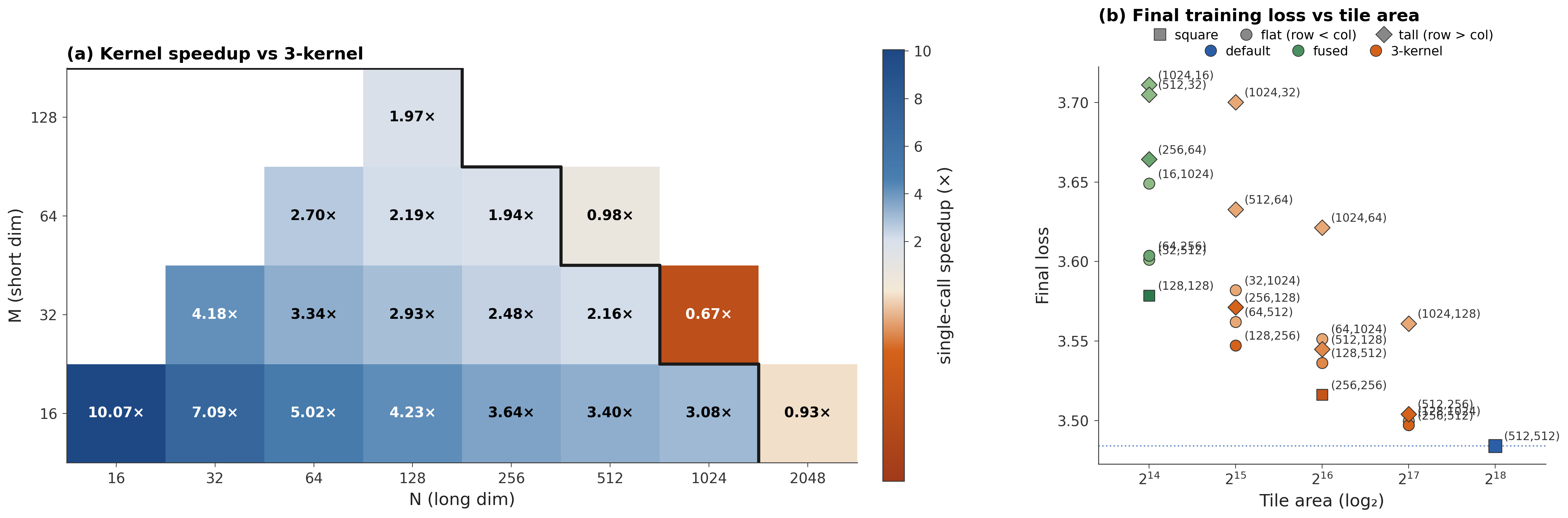
9 shows that kernel speed alone is not sufficient to select a tile shape. Smaller or more rectangular tiles can improve isolated kernel speed, but may worsen training loss in this diagnostic. In the tested setting, square tiles give a more favorable quality–speed trade-off than highly rectangular tiles. We therefore use square \(T=512\) tiles as the default on A40.
6.4 Cross-Layer Batching↩︎
We next evaluate the cross-layer batching strategy described in 4.4.2. This experiment separates the gain from tiling itself from the additional gain obtained by aggregating many independent tile computations into larger GPU launches.
In Qwen3-1.7B, there are \(28\) transformer blocks and \(7\) Muon-eligible matrices per block, giving \(196\) independent per-layer Newton–Schulz calls in an unbatched implementation. With \(T=512\), each individual matrix contains only a modest number of tiles, so launching one Newton–Schulz call per matrix can underutilize the GPU. Cross-layer batching groups compatible tiles across layers and processes them in a small number of larger batched calls.
Tiles of the same shape and dtype are grouped across layers and concatenated into a batched buffer. When the buffer exceeds the memory budget, it is split into the fewest chunks that fit, with intermediate workspace reused across steps. At \(T=512\), the \(1680\) tiles of Qwen3-0.6B fit in a single call, whereas the \(5376\) tiles of Qwen3-1.7B are processed in two chunks of \(2688\). In this benchmark, every optimizer is run on the same synthetic workload: \(8\) stacked bias-free Linear(\(H\),\(H\)) layers in bf16, fed fresh random Gaussian gradients at each step. HiMuon uses \(T=512\) and \(K=5\). Per-step time is the median over \(50\) steps after \(20\) warmup steps, and peak memory is the maximum allocated over a short run. The cross-layer variant additionally captures the batched Newton–Schulz workspace in a CUDA
graph, which pools and reuses that workspace across steps.
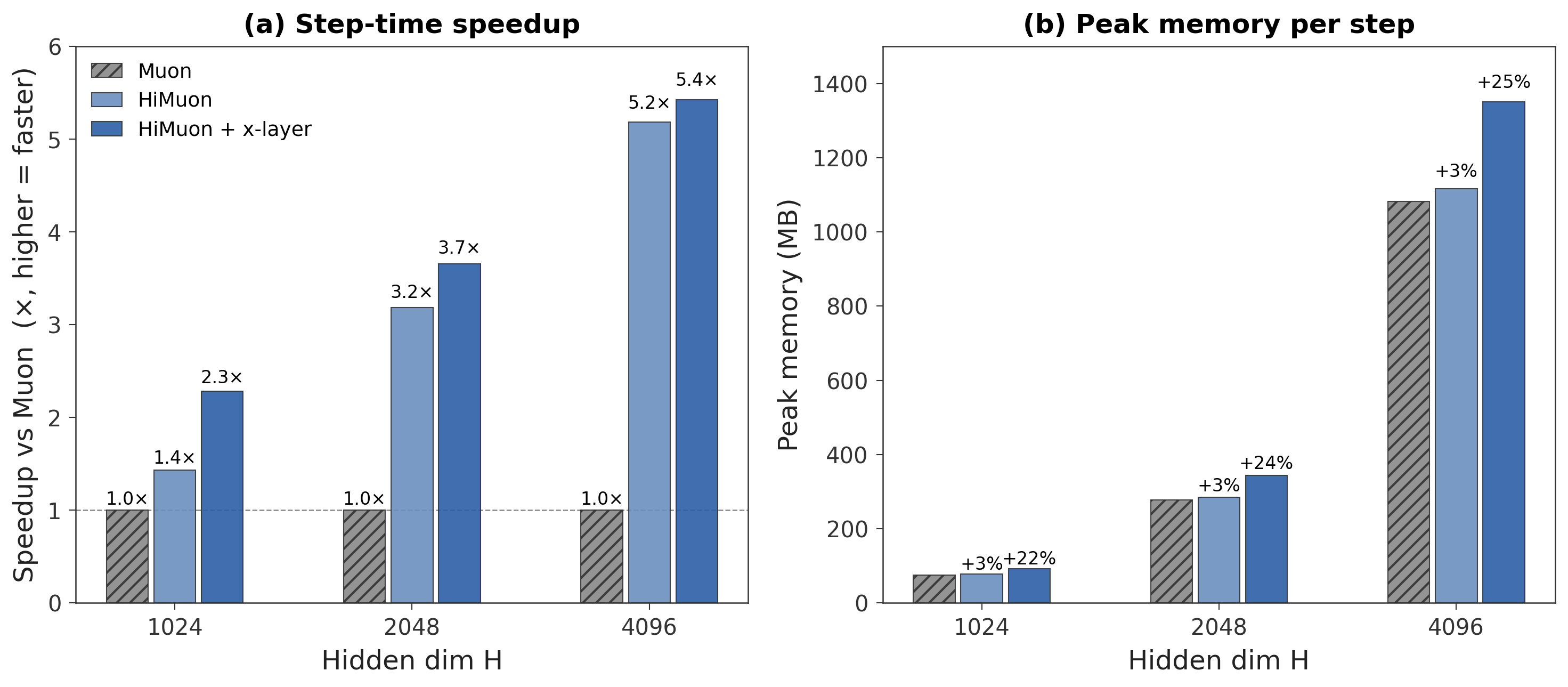
10 shows that the tiled map provides the dominant optimizer-step speedup. Cross-layer batching gives an additional wall-clock reduction by replacing many small Newton–Schulz calls with fewer larger batched calls. The incremental benefit is largest at \(H=1024\), where the plain tiled calls are small; it shrinks at \(H=4096\), where each call is already large enough to better utilize the GPU. The batching buffer increases peak memory, but the overhead is controlled by chunking and workspace reuse and does not grow with the number of training steps.
6.5 Capacity Robustness to Low Precision↩︎
Low-precision arithmetic in the Newton–Schulz inner GEMM is attractive on modern accelerators, but it perturbs the matrix-function update through rounding error [34]. We assess whether this perturbation changes the optimizer’s behavior on a controlled downstream metric. Using the one-step associative-memory benchmark of 5, we hold the problem instance and gradient fixed within each seed and vary only the GEMM precision used inside the Newton–Schulz iteration. Thus differences in recovered items reflect finite-precision arithmetic in the map rather than a different problem instance or tuned learning rate.
The setup uses \(d=1024\), \(N=4096\) keys, Zipf exponent \(\alpha=1.5\), batch-to-dimension ratio \(B/d=10\), \(K=5\) Newton–Schulz iterations, and five random seeds, executed on a single NVIDIA L40S. For each seed, the key–value pairs \((v_i,u_i)\sim\mathcal{N}(0,d^{-1}\mathbf{I}_d)\) and the resulting minibatch gradient \(\mathbf{G}_0\) are constructed in fp64 and held fixed across precision variants. The four precision settings are an fp64 reference, fp32, bf16, and fp8e4m3 with per-tensor scaling. The learning rate \(\eta=1.0\) is chosen once from the fp64 reference run and reused for every precision. We compare full-matrix Muon and HiMuon with \(T\in\{128,256,512\}\).
| Recovered items | Op.gap \(\delta_F\) to fp64 | |||||
|---|---|---|---|---|---|---|
| 2-5 (lr)6-7 Method | fp64 | fp32 | bf16 | fp8e4m3 | bf16 | fp8e4m3 |
| Muon | \(517.8\!\pm\!11.3\) | \(517.8\!\pm\!11.3\) | \(517.4\!\pm\!11.7\) | \(517.2\!\pm\!11.4\) | 0.062 | 0.019 |
| HiMuon-\(512\) | \(508.8\!\pm\!12.1\) | \(508.8\!\pm\!12.1\) | \(508.2\!\pm\!11.8\) | \(509.0\!\pm\!11.9\) | 0.061 | 0.027 |
| HiMuon-\(256\) | \(486.4\!\pm\!12.6\) | \(486.4\!\pm\!12.6\) | \(486.4\!\pm\!11.2\) | \(485.8\!\pm\!12.6\) | 0.058 | 0.039 |
| HiMuon-\(128\) | \(408.0\!\pm\!15.3\) | \(408.0\!\pm\!15.3\) | \(406.6\!\pm\!15.6\) | \(406.8\!\pm\!14.6\) | 0.052 | 0.059 |
3 shows that, for every update rule, the recovered item counts agree across precision settings to well within the seed-to-seed standard deviation. fp32 reproduces the fp64 means exactly under this setup. bf16 and fp8e4m3 produce operator-level gaps of roughly \(2\%\)–\(6\%\) relative to the per-method fp64 reference, yet change the mean recovered count by at most about one item out of roughly \(400\)–\(520\) recovered items. This is much smaller than the seed-to-seed standard deviation of roughly \(11\)–\(16\) items. Thus, in this diagnostic, using bf16 or fp8e4m3 for the Newton–Schulz inner GEMMs does not measurably change the downstream recovery metric.
6.6 Alignment and Descent Potential under Low Precision↩︎
The recovery test in 6.5 examines one downstream metric. We also evaluate two local quantities associated with per-step progress of Muon-type updates: the alignment \(\gamma\) of the update with the true gradient and the descent potential \(\phi\) along the update direction, as studied by Shumaylov et al. [35]. This experiment asks whether tile size and low-precision Newton–Schulz arithmetic change these quantities on a controlled quadratic proxy.
We write \(\langle\mathbf{A},\mathbf{B}\rangle_F=\mathop{\mathrm{tr}}(\mathbf{A}^\top\mathbf{B})\) for the Frobenius inner product. Given a full-batch gradient \(\mathbf{G}\), a minibatch gradient \(\widetilde{\mathbf{G}}\), an update direction \(\mathbf{D}\), and Hessian action \(\mathcal{H}[\mathbf{D}]\), define \[\gamma = \frac{\langle\mathbf{G},\mathbf{D}\rangle_F}{\langle\widetilde{\mathbf{G}},\mathbf{D}\rangle_F}, \qquad \phi = \frac{\langle\widetilde{\mathbf{G}},\mathbf{D}\rangle_F^2}{\langle\mathbf{D},\mathcal{H}[\mathbf{D}]\rangle_F}.\] Larger values correspond to faster local progress under an appropriately tuned step size. We evaluate these quantities on a teacher–student quadratic least-squares proxy after Davis and Drusvyatskiy [36]: \[f(\mathbf{W}) = \frac{1}{2} \mathbb{E}_{\boldsymbol{x}\sim\mathcal{N}(0,\boldsymbol{\Sigma})} \left\|(\mathbf{W}-\mathbf{W}^\star)\boldsymbol{x}\right\|^2 .\] The anisotropic covariance \(\boldsymbol{\Sigma}\) and teacher \(\mathbf{W}^\star\) yield the full gradient, minibatch gradient, and Hessian action in closed form.
Protocol. We use \(d=1024\), spectrum \(\lambda_i\propto i^{-\alpha}\) with \(\alpha=1\) and unit mean, a random orthogonal eigenbasis, minibatch size \(B=256\), and one seed. The teacher \(\mathbf{W}^\star\) and initial iterate are random unit-Frobenius matrices. A single fp32 full-matrix Muon trajectory of \(40\) steps (\(\eta=0.03\), unit-Frobenius-normalized update) generates the iterates. At each step, every tile-size and precision variant sees the same minibatch gradient \(\widetilde{\mathbf{G}}\). The evaluated update is \(\mathbf{D}=\Phi_{K,T}(\widetilde{\mathbf{G}})\) for \(T\in\{128,256,512\}\), or the full map \(\Phi_K(\widetilde{\mathbf{G}})\) on the full \(1024\times1024\) matrix, with \(K=5\). The map is evaluated in fp32, bf16, and fp8e4m3 with per-tile dynamic scaling on an NVIDIA L40S.
![Figure 11: Update alignment \gamma (left) and descent potential \phi (right) along a 40-step fp32 full-matrix Muon trajectory on a teacher–student quadratic proxy after Davis and Drusvyatskiy [36]. The setup uses d=1024, \alpha=1, B=256, K=5, one seed, and an NVIDIA L40S. Line color encodes the Newton–Schulz operator, from T=128 to T=512 and the full 1024\times1024 map. Precision is overlaid as bf16 circles and fp8 crosses on the fp32 line, sampled every fourth step.](/article/2606.27216/figures/microbench_precision_descent.png "fig:")
11 shows that both \(\gamma\) and \(\phi\) decline along the trajectory as the iterate approaches the teacher. The precision variants are visually indistinguishable at the plotted resolution: bf16 and fp8 markers lie on the corresponding fp32 curves for each tile size. Tile size has a more visible effect. The alignment curves remain close across tile sizes, while the descent-potential curves follow the ordering \(\text{full}>512>256>128\), with the largest gap early in the trajectory. This matches the qualitative ordering seen in the capacity diagnostic of 5.2. These results suggest that, in this controlled proxy, tile size changes the local update geometry more than the tested Newton–Schulz GEMM precisions.
7 Conclusion↩︎
In this paper, we introduced HiMuon, a tiled Newton–Schulz update for Muon-type optimization. HiMuon replaces one full-matrix Newton–Schulz map by independent applications of the same finite map on fixed-size intra-matrix tiles. This defines a local matrix-function update whose tile size controls the trade-off between retained spectral coupling and computational cost. For fixed \(T\), the leading Newton–Schulz work scales as \(\mathcal{O}(HWTK)\) rather than \(\mathcal{O}(HW\min\{H,W\}K)\).
The experiments characterize this trade-off at several levels. Capacity diagnostics show that larger tiles more closely preserve the behavior of full-matrix Muon, while smaller tiles reduce cost. GPU experiments show that the tiled formulation can be implemented efficiently through tile-size-dependent kernels, cross-layer batching, and memory-bounded chunking. End-to-end Qwen3 training experiments indicate that HiMuon reduces optimizer-step and wall-clock time while maintaining training and validation losses close to full-matrix Muon in the tested single-seed runs.
Future work includes a theory of the tiled map, adaptive schedules that choose \(T\) from training state or layer shape, and broader evaluation across model families, hardware platforms, and distributed training layouts.
Acknowledgments↩︎
The authors acknowledge the Minnesota Supercomputing Institute (MSI) at the University of Minnesota for providing the computational resources on which the majority of the experiments in this paper were run. The authors thank the developers of the Muon optimizer for making their implementation publicly available.
References↩︎
Department of Computer Science and Engineering, University of Minnesota, Minneapolis (, ). The research of Tang and Saad is supported by the NSF award DMS-2513117.↩︎
Department of Mathematics, Emory University, Atlanta, GA 30322 (, ). The research of Xi and Xu is supported by NSF award DMS-2513118.↩︎