The Observer World: A Cryptographic Extension of Impagliazzo’s Five Worlds
June 25, 2026
Abstract
Impagliazzo’s five worlds classify computational assumptions along a single axis, the existence of cryptographic primitives. All five worlds implicitly assume that every party, including the adversary, observes the full input, that the observer is always \(O_{\top}\). This assumption is so natural that it is never stated. This work makes it explicit and relaxes it by introducing a second, orthogonal axis, the observational axis, defined by the observer hierarchy of [1]. Relaxing the assumption reveals structural phenomena, such as the collapse \(\mathbf{P}_{O_{\mathrm{prof}}} = \mathbf{NP}_{O_{\mathrm{prof}}} \subsetneq \mathbf{P}\), that the five-world framework cannot express. We prove that this collapse holds unconditionally in all five worlds, showing that observational blindness and computational hardness are independent. We define the Observer World \(W_O\), classify all world-observer pairs, identify the labeled cells (a)–(d), and introduce a parametric family \(W_O^\varepsilon\) modelling partial violations of observational invariants. The framework also interfaces with physical information limits, including thermodynamic, quantum, and cosmological bounds.
1 Introduction↩︎
Impagliazzo’s five worlds [2] provide the most influential framework for reasoning about the gap between average-case and worst-case complexity, and about the foundations of cryptography. The five worlds \(\mathsf{Algorithmica}\), \(\mathsf{Heuristica}\), \(\mathsf{Pessiland}\), \(\mathsf{Minicrypt}\), \(\mathsf{Cryptomania}\) are defined by progressively stronger assumptions about the existence of computational hardness, from a world where \(\mathsf{P} = \mathsf{NP}\) to a world where public-key cryptography is possible.
Every one of the five worlds makes an implicit assumption that has not been made explicit in the five-world framework: that every party, including the adversary, has complete access to the input. In the language of [1], all five worlds assume that the observer is always \(O_{\top}\), the identity function on strings. This assumption is so natural in the computational setting that it is never stated.
This paper makes it explicit and relaxes it.
The observer theory of [1] introduces a partial order on functions \(O : \Sigma^* \to S\) that map inputs to observations, and proves that when the observer is structurally constrained (i.e.\(O \prec O_{\top}\)), the class of languages decidable under \(O\) depends on \(O\) alone and not on the nondeterministic power of the machine. In particular, the structural collapse \[\mathbf{P}_{O_{\mathrm{prof}}} = \mathbf{NP}_{O_{\mathrm{prof}}} \subsetneq \mathbf{P}\] holds unconditionally [1]: it is not a resolution of \(\mathsf{P}\) vs \(\mathsf{NP}\), but evidence that the distinction between computational hardness and structural blindness is real and independent of any computational assumption.
Since this result is unconditional, it holds in all five worlds simultaneously. The five worlds do not have the vocabulary to express it: they parametrise the computational axis but leave the observational axis fixed at \(O_{\top}\). In this sense the five worlds do not suffice: they describe variations along a line, while the observational axis exists orthogonally, and its structure is invisible from within any of the five worlds.
1.0.0.1 Cryptographic motivation.
In every cryptographic security argument, the adversary sees a ciphertext. The five worlds model computational power but say nothing about what the adversary sees: they implicitly assume \(O_{\top}\). The observational axis makes this explicit. Each labeled cell (a)–(d) of the world-observer table identifies a cryptographic phenomenon that the five-world framework cannot express: the observational collapse below the \(\mathsf{P}/\mathsf{NP}\) gap in every world including \(\mathsf{Algorithmica}\) (cell (a)), the non-additivity of computational hardness and observational blindness (cell (b)), a structural lower bound on one-way functions (cell (c)), and perfect secrecy as \(O_{\bot}\)-blindness on the plaintext (cell (d)).
1.0.0.2 Main contributions.
We prove that the structural collapse \(\mathbf{P}_{O_{\mathrm{prof}}} = \mathbf{NP}_{O_{\mathrm{prof}}} \subsetneq \mathbf{P}\) holds unconditionally in all five worlds simultaneously (Proposition 4), and classify the world-observer table, identifying four cells (a)–(d) that each witness a cryptographic phenomenon invisible to the five-world framework (Section 4).
We define the Observer World \(W_O\) formally as a sixth landscape (Definition 5) and prove it is not reducible to any of the five worlds (Proposition 14, Section 5).
We introduce the parametric family \(W_O^\varepsilon\) with invariant violation parameter \(\varepsilon\in [0,1]\), modelling worlds in which an adversary partially circumvents observational blindness, and identify the most informationally rich cell: \(\mathsf{Pessiland}\times O_{\mathrm{prof}}\times \varepsilon> 0\) (Section 6).
We identify connections between the Observer World framework and physical information limits, thermodynamic, quantum, and cosmological, and state precise open problems formalising each connection (Section 7).
1.0.0.3 Limitations.
The author is a computer scientist, not a physicist. The physical connections of Section 7 are stated as open problems and conjectures, not theorems; no physical conclusions are claimed beyond what the mathematical framework directly implies. All machines in this paper are standard multi-tape deterministic or nondeterministic Turing machines over \(\{0,1\}^*\); the observer is a fixed preprocessing map applied before any machine computation begins (see Remark 1). The parametric family \(W_O^\varepsilon\) (Section 6.2) requires an information metric whose precise formulation is an open direction (Section 7.1, Open Problem 28).
2 Preliminaries: canonical observers↩︎
We recall the definitions and results from [1] used throughout this paper. All machines are standard multi-tape Turing machines. An observer \(O : \Sigma^* \to S\) is a fixed total function applied once to the input before any machine computation begins; it does not interact with the machine and does not extend the computational model.
Remark 1 (Machine model). \(\mathbf{P}_{O}\) consists of languages decidable in time polynomial in \(|\mathrm{enc}(O(x))|\) by a deterministic TM receiving \(\mathrm{enc}(O(x))\) as its entire input, where \(\mathrm{enc} : S \to \{0,1\}^*\) is a fixed canonical injective encoding. \(\mathbf{NP}_{O}\) is defined analogously with a nondeterministic TM and a polynomial-length certificate. For \(O = O_{\top}\) these reduce to standard \(\mathbf{P}\) and \(\mathbf{NP}\) [1]. The observer only reduces available information and never increases computational power [1]. Throughout this paper we identify \(O(x)\) with \(\mathrm{enc}(O(x))\) and write, e.g., “the TM receives \(O(x)\)” as shorthand for “the TM receives \(\mathrm{enc}(O(x))\)”; all complexity bounds are in terms of \(|\mathrm{enc}(O(x))|\).
Definition 1 (Canonical observers [1]). Let \(\Sigma = \{0, 1\}\) (see Remark 2). The canonical observers are:
\(O_{\bot}: \Sigma^* \to \{\star\}\), \(O_{\bot}(x) = \star\) for all \(x\). Map: constant map. Invariant: discards all information. Decidable class: \(\mathcal{L}(O_{\bot}) = \{\emptyset, \Sigma^*\}\) by [1].
\(O_{\mathrm{len}}: \Sigma^* \to \mathbb{N}\), \(O_{\mathrm{len}}(x) = |x|\). Map: string length. Invariant: length-determined languages. Decidable class: all \(L\) with \(x \in L \iff |x| \in I\) for some \(I \subseteq \mathbb{N}\).
\(O_{\mathrm{par}}: \Sigma^* \to \{0,1\}^2\), \(O_{\mathrm{par}}(x) = (|x|_0 \bmod 2,\, |x|_1 \bmod 2)\). Map: symbol-count parities. Invariant: parity of each symbol count. Decidable class: all \(L\) determined by symbol-count parities.
\(O_{\mathrm{prof}}: \Sigma^* \to \mathbb{N}^2\), \(O_{\mathrm{prof}}(x) = (|x|_0, |x|_1)\) (the profile of \(x\)). Map: symbol counts. Invariant: permutation-closure. Decidable class: all permutation-closed languages [1].
\(O_k : \Sigma^* \to \mathcal{P}(\Sigma^{\leq k})\), where \(O_k(x)\) is the set of subsequences of \(x\) of length \(\leq k\) (\(k \geq 1\)). Map: \(k\)-subsequence set. Invariant: \(k\)-piecewise testability. Decidable class: all \(k\)-piecewise testable languages (Simon’s hierarchy [1]).
\(O_{\top}: \Sigma^* \to \Sigma^*\), \(O_{\top}(x) = x\). Map: identity. Invariant: none (full information). Decidable class: all languages.
Remark 2 (Alphabet convention). Definition 1 uses \(\Sigma = \{0,1\}\) for concreteness. For a general \(k\)-symbol alphabet \(\Sigma = \{a_0,\dots,a_{k-1}\}\), replace \((|x|_0, |x|_1)\) with \((|x|_{a_0},\dots,|x|_{a_{k-1}}) \in \mathbb{N}^k\). All order relations and separation witnesses carry over unchanged [1].
The following table summarises the canonical observers.
| Observer | Map \(O(x)\) | Key invariant | Example \(L \in \mathcal{L}(O)\) | \(\mathbf{P}_{O} = \mathbf{NP}_{O}\)? |
|---|---|---|---|---|
| \(O_{\bot}\) | \(\star\) | all | \(\emptyset\) | yes (trivially) |
| \(O_{\mathrm{len}}\) | \(|x|\) | length | \(\{x \mid |x|\;\text{even}\}\) | open |
| \(O_{\mathrm{par}}\) | parities of counts | symbol parities | \(\{x \mid |x|_1 \equiv 0\}\) | open |
| \(O_{\mathrm{prof}}\) | \((|x|_0, |x|_1)\) | perm.-closure | \(\{x \mid |x|_0 = |x|_1\}\) | yes (structurally) |
| \(O_k\) | \(k\)-subsequence set | \(k\)-p.t. | \(\{x \mid 01 \sqsubseteq x\}\) | open |
| \(O_{\top}\) | \(x\) | none | \(0^*1^*\) | open (P vs NP) |
The partial order \(\preceq\) on observers is defined by [1]: \(O_1 \preceq O_2\) if there exists a function \(f\) with \(O_1 = f \circ O_2\). The complete order relations among the canonical observers are: \[\begin{align} &O_{\bot}\prec O_{\mathrm{len}}\prec O_{\mathrm{prof}}\prec O_{\top}, \\ &O_{\bot}\prec O_{\mathrm{par}}\prec O_{\mathrm{prof}}\prec O_{\top}, \\ &O_{\bot}\prec O_1 \prec O_2 \prec \cdots \prec O_{\top}, \end{align}\] with \(O_{\mathrm{len}}\) and \(O_{\mathrm{par}}\) incomparable, and \(O_{\mathrm{prof}}\) incomparable with every \(O_k\) [1].
A language \(L \subseteq \Sigma^*\) is \(O\)-saturated (Definition 3.2 of [1], also called \(O\)-invariant) if \(O(x) = O(y)\) implies \(x \in L \iff y \in L\), where we write \(x \sim_O y\) to denote the equivalence relation \(O(x) = O(y)\). Equivalently, \(L\) is \(O\)-saturated if it is a union of \(\sim_O\)-equivalence classes, or if membership in \(L\) is determined entirely by \(O(x)\). We use both terms interchangeably throughout the paper.
3 The five worlds and their silent assumption↩︎
We recall the five worlds of Impagliazzo [2] and make their shared implicit assumption explicit.
Definition 2 (Impagliazzo’s five worlds [2]).
\(\mathsf{Algorithmica}\): \(\mathsf{P} = \mathsf{NP}\). Every problem in \(\mathsf{NP}\) is solvable in polynomial time.
\(\mathsf{Heuristica}\): \(\mathsf{P} \neq \mathsf{NP}\) but no NP problem is hard on average: every NP problem has a polynomial-time algorithm that succeeds on all but a negligible fraction of instances under any efficiently samplable distribution.
\(\mathsf{Pessiland}\): NP problems are hard on average, but one-way functions do not exist: no function is hard to invert on average.
\(\mathsf{Minicrypt}\): one-way functions exist, but public-key cryptography does not: no key-exchange protocol is secure against a computationally bounded adversary.
\(\mathsf{Cryptomania}\): public-key cryptography exists: there exist functions that are easy to compute but hard to invert even given additional public information (trapdoor one-way functions).
Remark 3 (The silent assumption). In every world of Definition 2, every machine, including the adversary, receives the complete input \(x\). In the language of [1], the observer is always \(O_{\top}: x \mapsto x\). This assumption is never stated in the five-world framework because it is universal and no party is ever observationally constrained. The five worlds vary the computational assumption (what is hard) but not the observational assumption (what is visible).
Proposition 4 (The observational collapse is world-independent). In every world \(W_i\) of Definition 2, the following holds unconditionally: \[\mathbf{P}_{O_{\mathrm{prof}}} = \mathbf{NP}_{O_{\mathrm{prof}}} \subsetneq \mathbf{P}.\]
Proof. By [1], this holds with no assumption on \(\mathsf{P}\) vs \(\mathsf{NP}\) and with no cryptographic assumption. Since the five worlds are defined by computational and cryptographic assumptions, and the collapse is independent of all such assumptions, it holds in every world of Definition 2.
We now sketch why the collapse holds. Any language in \(\mathbf{P}_{O_{\mathrm{prof}}}\) has membership determined solely by \(O_{\mathrm{prof}}(x) = (|x|_0, |x|_1)\). A TM under \(O_{\mathrm{prof}}\) receives \(O_{\mathrm{prof}}(x)\) as its entire input, a string of length \(O(\log|x|)\). Any nondeterministic certificate must also be a function of this input alone; it cannot depend on \(x\) itself (which the machine does not receive). Hence a nondeterministic TM under \(O_{\mathrm{prof}}\) decides exactly the same languages as a deterministic one: \(\mathbf{P}_{O_{\mathrm{prof}}} = \mathbf{NP}_{O_{\mathrm{prof}}}\). The language \(L_0 = 0^*1^*\) is in \(\mathbf{P}\) (one linear scan) but not \(O_{\mathrm{prof}}\)-decidable: \(O_{\mathrm{prof}}(01) = O_{\mathrm{prof}}(10) = (1,1)\) while \(01 \in L_0\) and \(10 \notin L_0\). Hence \(\mathbf{P}_{O_{\mathrm{prof}}} \subsetneq \mathbf{P}\). Full proof in [1]. ◻
Remark 5 (What Proposition 4 says). Proposition 4 does not say that \(\mathsf{P} = \mathsf{NP}\) holds in all five worlds: it says that a different collapse, one that places \(\mathbf{P}_{O_{\mathrm{prof}}}\) strictly below \(\mathbf{P}\) in the language containment order, due to structural blindness rather than computational coincidence, holds regardless of where we are in the five-world landscape. The five worlds cannot distinguish between a problem that is computationally hard and a problem that is not well-posed for a given observer; Proposition 4 shows that these two phenomena are genuinely independent.
4 The world-observer table↩︎
We construct the table of all pairs \((W_i, O)\) where \(W_i\) is one of the five worlds and \(O\) is a canonical observer of [1]. We first formalise the notions of a labeled cell and cell reduction.
Definition 3 (Non-trivial cell). A cell \((W_i, O)\) of the world-observer table is non-trivial if there exists a language \(L \in \mathbf{P}_{O_{\top}} \setminus \mathbf{P}_{O}\), i.e.if the observational constraint strictly reduces the class of decidable languages. A cell is trivial if \(\mathbf{P}_{O} = \mathbf{NP}_{O} = \{\emptyset, \Sigma^*\}\), which holds whenever \(O \preceq O_{\bot}\) [1].
Note. We call cells (a)–(d) the labeled cells of the table: they are the cells singled out for individual analysis below. Cells (a)–(c) are non-trivial in the formal sense above. Cell (d) (\(\mathsf{Cryptomania}\times O_{\bot}\)) is formally trivial (\(\mathbf{P}_{O_{\bot}} = \{\emptyset, \Sigma^*\}\)), but is labelled separately in the table because the world \(\mathsf{Cryptomania}\) contains public-key primitives that create a cryptographically meaningful contrast with the classical cell \((\mathsf{Cryptomania}, O_{\top})\); this distinction is invisible to the formal condition above and is explained in the legend below.
Definition 4 (Cell reduction). We say cell \((W_i, O)\) many-one reduces to \((W_j, O')\) if there exists a polynomial-time computable map \(T : \Sigma^* \to \Sigma^*\) such that for every language \(L\) decidable in \((W_i, O)\), there exists a language \(L'\) decidable in \((W_j, O')\) with \(x \in L \iff T(x) \in L'\) for all \(x\), and \(T\) preserves observational transcripts: \(O(x) = O'(T(x))\) for all \(x\). Cell reductions are not used in the proofs of this paper; the definition is included to make precise the sense in which cells are independent that is implicit in Proposition 14.
4.1 The table↩︎
| \(O_{\bot}\) | \(O_{\mathrm{len}}\)/\(O_{\mathrm{par}}\) | \(O_{\mathrm{prof}}\) | \(O_k\) | \(O_{\top}\) | |
|---|---|---|---|---|---|
| \(\mathsf{Algorithmica}\) | trivial | trivial | (a) | standard | classical |
| \(\mathsf{Heuristica}\) | trivial | trivial | (a) | standard | classical |
| \(\mathsf{Pessiland}\) | trivial | trivial | (b) | standard | classical |
| \(\mathsf{Minicrypt}\) | trivial | trivial | (c) | standard | classical |
| \(\mathsf{Cryptomania}\) | (d) | trivial | (a) | standard | classical |
Legend. Trivial: \(\mathbf{P}_{O} = \mathbf{NP}_{O} = \{\emptyset, \Sigma^*\}\) by [1]; computational assumptions are irrelevant. Standard: Simon’s hierarchy applies; see [1]. Classical: \(\mathbf{P}_{O_{\top}} = \mathbf{P}\) and \(\mathbf{NP}_{O_{\top}} = \mathbf{NP}\); the standard five-world analysis applies [2]. Cells (a)–(c) are non-trivial in the sense of Definition 3 and are treated in Section 4.2. Cell (d) (\(\mathsf{Cryptomania}\times O_{\bot}\)) is formally trivial by Definition 3 but is labelled separately because, as explained in the note within Definition 3 and below, the world \(\mathsf{Cryptomania}\) creates a cryptographically distinct situation for an \(O_{\bot}\)-blind adversary. All other \(O_{\bot}\) cells are listed as trivial: they share the structural property \(\mathbf{P}_{O_{\bot}} = \{\emptyset, \Sigma^*\}\) and their computational world creates no analogous contrast. The cell \((\mathsf{Cryptomania}, O_{\bot})\) is the sole \(O_{\bot}\) entry worth distinguishing: in \(\mathsf{Cryptomania}\), an adversary with \(O_{\top}\) could exploit public-key primitives, while one with \(O_{\bot}\) cannot even pose the question of which plaintext was encrypted. It is this contrast, absent in all other worlds, that motivates its separate label.
4.2 The labeled cells (a)–(d)↩︎
Proposition 6 (Cell (a): any world \(\times\) \(O_{\mathrm{prof}}\)). In every world \(W_i\): \[\mathbf{P}_{O_{\mathrm{prof}}} = \mathbf{NP}_{O_{\mathrm{prof}}} \subsetneq \mathbf{P}_{O_{\top}} = \mathbf{P}.\] If additionally \(\mathsf{P} \neq \mathsf{NP}\) (which is assumed in all worlds except \(\mathsf{Algorithmica}\)): \[\mathbf{NP}_{O_{\mathrm{prof}}} = \mathbf{P}_{O_{\mathrm{prof}}} \subsetneq \mathbf{P} \subsetneq \mathbf{NP}.\] The observational collapse occurs strictly below the \(\mathsf{P}\)/\(\mathsf{NP}\) gap, on the opposite side from \(\mathsf{NP}\).
Proof. Unconditional part: Proposition 4. Conditional part: combining with \(\mathbf{P} \subsetneq \mathbf{NP}\) under the assumption \(\mathsf{P} \neq \mathsf{NP}\). ◻
4.2.0.1 Toy example for cell (a).
Let \(L = \{x \in \{0,1\}^* \mid x_1 = 1\}\) (strings whose first symbol is \(1\)). For any \(x, x'\) with \(O_{\mathrm{prof}}(x) = O_{\mathrm{prof}}(x')\) we can have \(x_1 = 1\) and \(x'_1 = 0\) (e.g.\(x = 10\), \(x' = 01\), both with profile \((1,1)\)). Hence \(L\) is not \(O_{\mathrm{prof}}\)-decidable. However, \(L \in \mathbf{P}\) (read the first symbol in \(O(1)\) time). This witnesses \(\mathbf{P}_{O_{\mathrm{prof}}} \subsetneq \mathbf{P}\) independently of any of the five worlds.
Remark 7. Cell (a) is the most important labeled cell. It shows that even in \(\mathsf{Algorithmica}\), where \(\mathsf{P} = \mathsf{NP}\), the observational collapse \(\mathbf{P}_{O_{\mathrm{prof}}} \subsetneq \mathbf{P}\) persists. The collapse is not cancelled by the strongest possible computational assumption. The observational and computational axes are orthogonal.
Proposition 8 (Cell (b): \(\mathsf{Pessiland}\times O_{\mathrm{prof}}\)). In \(\mathsf{Pessiland}\):
NP problems are hard on average, but no one-way function exists.
An adversary with observer \(O_{\mathrm{prof}}\) cannot pose any problem that depends on the ordering of input symbols: such problems are not \(O_{\mathrm{prof}}\)-saturated and are not well-formed in the adversary’s observation space.
The hardness in \(\mathsf{Pessiland}\) and the blindness of \(O_{\mathrm{prof}}\) interact non-additively: problems that are hard on average in \(\mathsf{Pessiland}\) may be problems that the \(O_{\mathrm{prof}}\) adversary cannot even recognise as distinct from trivial ones.
There is no cryptographic security in \(\mathsf{Pessiland}\) (no one-way functions), but the adversary with \(O_{\mathrm{prof}}\) faces a different limitation: structural blindness to ordering. These two limitations are independent; neither implies the other.
Proof. Parts (i) and (iv): by definition of \(\mathsf{Pessiland}\) [2].
Part (ii): by [1], a language is decidable under \(O_{\mathrm{prof}}\) if and only if it is permutation-closed; languages depending on ordering are not permutation-closed and hence not \(O_{\mathrm{prof}}\)-decidable, regardless of computational power.
Part (iii): the hardness of NP problems in \(\mathsf{Pessiland}\) is a property of the problem as seen by an \(O_{\top}\) adversary. An \(O_{\mathrm{prof}}\) adversary does not see the same problem: ordering-dependent difficulty is invisible to it. The two phenomena apply to different parts of the problem landscape and do not combine additively. ◻
4.2.0.2 Toy example for cell (b).
The following example illustrates the independence between observational blindness and average-case hardness, not their co-occurrence. Consider the problem: given \(x \in \{0,1\}^*\), determine whether \(x\) is the lexicographically sorted version of its symbols (all \(0\)s precede all \(1\)s). This problem is in \(\mathbf{P}\) (one linear scan), not NP-hard, and not hard on average. Nevertheless, an \(O_{\mathrm{prof}}\) adversary sees only \((|x|_0, |x|_1)\) and cannot distinguish \(0^a 1^b\) from any other string with the same profile; the problem is therefore not \(O_{\mathrm{prof}}\)-decidable. This shows that ordering-dependence and \(O_{\mathrm{prof}}\)-blindness are independent of the computational difficulty of the problem: a problem can be easy (in \(\mathbf{P}\)), ordering-dependent, and \(O_{\mathrm{prof}}\)-invisible simultaneously. The same independence holds for NP-hard ordering-dependent problems in \(\mathsf{Pessiland}\): their hardness is a property relative to \(O_{\top}\), not a property that \(O_{\mathrm{prof}}\) can detect.
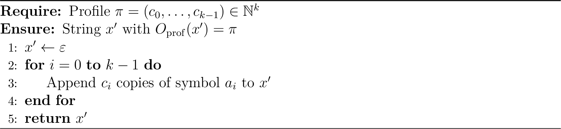
Lemma 1 (Profile preimage construction). Given a profile \(\pi = (c_0, \dots, c_{k-1}) \in \mathbb{N}^k\) with \(n = \sum_{i=0}^{k-1} c_i\), Algorithm 1 constructs a string \(x' \in \Sigma^*\) with \(O_{\mathrm{prof}}(x') = \pi\) in time \(O(n)\). Full proof in Appendix 10.
Proposition 9 (Cell (c): \(\mathsf{Minicrypt}\times O_{\mathrm{prof}}\)). In \(\mathsf{Minicrypt}\), where one-way functions exist:
No one-way function \(f : \Sigma^* \to \Sigma^*\) can be \(O_{\mathrm{prof}}\)-saturated.
Equivalently, every one-way function that exists in \(\mathsf{Minicrypt}\) must depend on the ordering of its input symbols in an essential way.
Proof. We use the general-alphabet form of \(O_{\mathrm{prof}}\) (Remark 2): for a \(k\)-symbol alphabet \(\Sigma = \{a_0, \dots, a_{k-1}\}\), \(O_{\mathrm{prof}}(x) = (|x|_{a_0}, \dots, |x|_{a_{k-1}}) \in \mathbb{N}^k\).
Part (i): suppose \(f\) is \(O_{\mathrm{prof}}\)-saturated and one-way. By [1], \(f(x)\) depends only on \(O_{\mathrm{prof}}(x) = (|x|_{a_0}, \dots, |x|_{a_{k-1}})\).
An adversary with \(O_{\top}\) who observes \(y = f(x)\) inverts \(f\) as follows. By the standard definition of one-way functions, the inverting algorithm receives \((1^n, y)\) where \(n = |x|\), so \(n\) is known. The adversary enumerates all profiles \(\pi \in \mathbb{N}^k\) with \(\sum_i \pi_i = n\) (at most \((n+1)^{k-1}\) many, polynomial in \(n\) for fixed \(k\)), and for each \(\pi\) evaluates \(f(\mathrm{ConstructFromProfile}(\pi))\) using Algorithm 1 and the publicly known \(f\). Since \(f\) is \(O_{\mathrm{prof}}\)-saturated, \(f\) takes the same value on every string sharing a profile; hence there exists some \(\pi^*\) among those enumerated with \(f(\mathrm{ConstructFromProfile}(\pi^*)) = y\). Setting \(x' = \mathrm{ConstructFromProfile}(\pi^*)\) gives a string satisfying \(f(x') = y\). The entire procedure runs in time polynomial in \(n\), contradicting the one-wayness of \(f\).
Part (ii): the contrapositive of part (i). If \(f\) is one-way in \(\mathsf{Minicrypt}\), then \(f\) is not \(O_{\mathrm{prof}}\)-saturated, which means \(f(x) \neq f(x')\) for some \(x, x'\) with \(O_{\mathrm{prof}}(x) = O_{\mathrm{prof}}(x')\). Hence \(f\) distinguishes permutations of the same input. ◻
Remark 10. Proposition 9 gives a structural lower bound on one-way functions: they must be ordering-sensitive. Any candidate one-way function that is invariant under permutation of its input, for example, any function of the Hamming weight alone, cannot be one-way, even in \(\mathsf{Minicrypt}\). This is a consequence of observational structure, not of any hardness assumption.
4.2.0.3 Toy example for cell (c).
Let \(f(x) = |x|_1\) (Hamming weight, interpreted as an integer). This function depends only on the symbol count \(|x|_1\), which is the second component of \(O_{\mathrm{prof}}(x) = (|x|_0, |x|_1)\); hence \(f\) is \(O_{\mathrm{prof}}\)-saturated. By Proposition 9(i), \(f\) cannot be one-way in \(\mathsf{Minicrypt}\). Indeed, to invert \(f\) on a value \(v\) for an input of length \(n = |x|\), Algorithm 1 constructs \(0^{n-v}1^v\) in \(O(n)\) time, giving a preimage with \(|x'|_1 = v\).
Proposition 11 (Cell (d): \(\mathsf{Cryptomania}\times O_{\bot}\)). In \(\mathsf{Cryptomania}\), an adversary with observer \(O_{\bot}\) on the plaintext space cannot recover any information about the plaintext from the ciphertext, for any encryption scheme.
Proof. Since \(O_{\bot}(m) = \star\) for all \(m\) (Definition 1(i)), a machine receiving only \(O_{\bot}(m)\) receives the same input \(\star\) regardless of \(m\). No machine, regardless of computational power, can distinguish any two plaintexts from \(\star\) alone: the adversary’s observation space contains no information about the plaintext. This is structural blindness: by [1], \(\mathbf{P}_{O_{\bot}} = \mathbf{NP}_{O_{\bot}} = \{\emptyset, \Sigma^*\}\). The existence of cryptographic primitives in \(\mathsf{Cryptomania}\) is irrelevant, since the adversary cannot even pose the question of which plaintext was encrypted. ◻
4.2.0.4 Toy example for cell (d): MR-OTP perfect secrecy.
Let \(B = (2, 3)\) and consider the MR-OTP [3] with message \(M = (m_1, m_2) \in \mathbb{Z}_2 \times \mathbb{Z}_3\) and key \(K = (k_1, k_2)\) uniform on \(\mathbb{Z}_2 \times \mathbb{Z}_3\). Ciphertext: \(C = ((m_1 + k_1) \bmod 2,\, (m_2 + k_2) \bmod 3)\). For any fixed \(c = (c_1, c_2)\) and any \(m\), the unique key mapping \(m\) to \(c\) is \(K = (c_1 - m_1 \bmod 2,\, c_2 - m_2 \bmod 3)\). Since \(K\) is uniform, \(\Pr[C = c \mid M = m] = 1/6\) for all \(m\) and \(c\). Hence \(\Pr[M = m \mid C = c] = \Pr[M = m]\): perfect secrecy [3]. The adversary’s observer on the plaintext is \(O_{\bot}\): the ciphertext carries zero information about \(m\).
Remark 12 (Cell (d) and the MR-OTP). Cell (d) describes the situation of an adversary facing the Mixed-Radix One-Time Pad [3] in the ciphertext-only setting (see Definition 5 in Section 5 for the formal definition of the Observer World and the adversary/defender asymmetry). By [3], the MR-OTP achieves Shannon perfect secrecy [4]: the ciphertext distribution is identical for every plaintext, placing the adversary in the \(O_{\bot}\)-on-plaintext situation of Proposition 11. This holds in every world \(W_i\), including \(\mathsf{Cryptomania}\): the perfect secrecy of the MR-OTP is not a consequence of the hardness assumptions of \(\mathsf{Cryptomania}\) but of the information-theoretic structure of the cipher. Even the strongest cryptographic adversary in \(\mathsf{Cryptomania}\) is reduced to \(O_{\bot}\) on the plaintext.
5 The Observer World: a sixth landscape↩︎
Definition 5 (Observer World). An Observer World is a pair \(W_O = (W_i, O)\) where \(W_i\) is one of the five worlds of Definition 2 and \(O : \Sigma^* \to S\) is an observer in the hierarchy of [1]. In \(W_O\):
The computational assumptions of \(W_i\) hold for all parties.
The adversary’s input is \(O(x)\), not \(x\): the adversary operates under observer \(O\) rather than \(O_{\top}\).
The defender’s input is \(O_{\top}(x) = x\): the defender has full access to the input.
Remark 13 (Cryptographic interpretation of the asymmetry). The asymmetry between adversary (\(O\)) and defender (\(O_{\top}\)) in Definition 5 is deliberate and models the cryptographic setting: the defender generates and knows the key, while the adversary observes only the ciphertext (or a more informative projection of the input, depending on the attack model). The case \(O = O_{\top}\) recovers the classical five-world framework with no observational constraint on the adversary.
The following lemma constructs, for any \(O \prec O_{\top}\), a language that is \(O\)-saturated but whose membership is independent of every five-world computational assumption.
Lemma 2 (Observationally invariant, computationally independent language). Let \(O \prec O_{\top}\). There exists a language \(L\) that is \(O\)-saturated and such that membership in \(L\) cannot be decided from any purely computational assumption about \(W_i\) alone. The language \(L\) constructed below may or may not belong to \(\mathbf{P}\) or \(\mathbf{NP}\); the lemma asserts only that its membership is independent of the five-world assumptions.
Proof sketch. Partition \(\Sigma^*\) into \(\sim_O\)-equivalence classes \([u_0]_O, [u_1]_O, \dots\), and let \(M_0, M_1, \dots\) enumerate all polynomial-time machines receiving \(O(x)\). For each \(e\), pick a canonical representative \(u_e^* \in [u_e]_O\) and define \([u_e]_O \subseteq L\) iff \(M_e\) rejects \(O(u_e^*)\) (a diagonalisation). The resulting \(L\) is a union of \(\sim_O\)-classes, hence \(O\)-saturated; by construction, no \(M_e\) decides \(L\) correctly, so \(L \notin \mathbf{P}_{O}\). The construction uses only the \(\sim_O\) relation (a property of \(O\) alone) and makes no assumption about \(\mathsf{P}\) vs \(\mathsf{NP}\), one-way functions, or public-key cryptography; hence membership in \(L\) is independent of all five-world computational assumptions. ◻
The full constructive proof is in Appendix 9.
Proposition 14 (The Observer World is not reducible to the five worlds). For \(O \prec O_{\top}\), the Observer World \(W_O = (W_i, O)\) is not equivalent to any of the five worlds \(W_j\) with observer \(O_{\top}\): no computational assumption about \(W_j\) implies the structural collapse \(\mathbf{P}_{O} = \mathbf{NP}_{O} \subsetneq \mathbf{P}\), and no observational constraint in \(W_O\) implies any of the computational assumptions of \(W_i\).
Proof. We exhibit the argument for \(O = O_{\mathrm{prof}}\); the general case \(O \prec O_{\top}\) follows by the same structure using Lemma 2 for arbitrary \(O\).
No computational assumption implies the observational collapse. The structural collapse \(\mathbf{P}_{O_{\mathrm{prof}}} = \mathbf{NP}_{O_{\mathrm{prof}}} \subsetneq \mathbf{P}\) is unconditional [1]: it holds regardless of which \(W_i\) contains us, and hence cannot be a consequence of any computational assumption. By Lemma 2, there exists a language \(L\) that is \(O_{\mathrm{prof}}\)-saturated and independent of all five-world assumptions; this witnesses the orthogonality of the two axes.
No observational constraint implies any computational assumption. The observational constraint \(O \prec O_{\top}\) is a statement about the information available to the adversary, not about the computational difficulty of any problem. By [1], computational hardness and observational saturation are independent: there exist languages in \(\mathbf{P}\) that are not \(O_{\mathrm{prof}}\)-saturated, and languages outside \(\mathbf{RE}\) that are \(O_{\mathrm{prof}}\)-saturated. The observational parameter \(O\) carries no information about the computational structure of \(W_i\). ◻
Remark 15 (The Observer World as a sixth world). Proposition 14 shows that the parameter \(O\) adds genuinely new content to the five-world framework: it cannot be encoded as a computational assumption within the existing five worlds. The Observer World \(W_O\) is therefore a sixth landscape, not a variation on an existing world, but an orthogonal dimension of the complexity landscape.
The analogy with Impagliazzo’s construction is structural. Impagliazzo introduced five worlds by varying a single parameter (the existence of one-way functions) along a single axis. We introduce the Observer World by varying a second parameter (the observer \(O\)) along a second axis. The resulting landscape is two-dimensional: the five-world axis (computational) and the observational axis.
6 Observer worlds with broken invariants↩︎
The Syntactic Invariance Principle (SIP) of [5] states that a syntactic system cannot derive clauses that violate a syntactic invariant. In the observational setting, the observer \(O\) defines an observational invariant: a language \(L\) is \(O\)-invariant (equivalently, \(O\)-saturated; see Section 2) if membership in \(L\) is determined entirely by \(O(x)\). An Observer World with observer \(O\) places the adversary within the observational invariant defined by \(O\): the adversary cannot access information that \(O\) discards.
An Observer World with broken invariant is one in which the adversary finds a mechanism to circumvent this constraint, the observational analogue of SIP violation.
6.1 Three cases of invariant violation↩︎
Definition 6 (Oracle violation). In an Observer World \(W_O = (W_i, O)\) with oracle violation, the adversary has observer \(O\) on the input but additionally has adaptive oracle access to queries \(q_1, q_2, \dots, q_d\) on \(x\), where each \(q_{j+1}\) may depend on the responses \((x[q_1], \dots, x[q_j])\). The adversary’s total observation is the pair \((O(x),\, (x[q_1], \dots, x[q_d]))\).
Remark 16 (Oracle violation and adaptive observers). As formalised in Remark 26 below (Section 7), an oracle queried adaptively is an adaptive observer of finite depth. Definition 6 is therefore the special case of an adaptive observer of depth \(d\) applied to an Observer World. The oracle-relative separations of the relativisation barrier [6] are separations in the hierarchy of adaptive Observer Worlds, not in the static observational hierarchy of [1].
Proposition 17 (Oracle violation and the MR-OTP). In the ciphertext-only setting of \(W_O = (W_i, O_{\bot})\), oracle access to the ciphertext \(C = \mathrm{Enc}(M, K)\) (where \(\mathrm{Enc}\) denotes MR-OTP encryption: \(C_i = (M_i + K_i) \bmod b_i\)) provides no information about the plaintext \(M\) for the MR-OTP [3], regardless of the number of oracle queries and regardless of which world \(W_i\) we are in.
Proof. By [3], the MR-OTP achieves perfect secrecy: for every plaintext \(M\) and every ciphertext \(c \in \mathcal{D}_B\), \(\Pr[C = c \mid M] = |\mathcal{D}_B|^{-1}\). In particular, \(C\) and \(M\) are independent random variables.
We prove by induction on depth \(d\) that the adaptive query transcript \((C[q_1], \dots, C[q_d])\) is independent of \(M\).
Base case (\(d = 0\)). The empty transcript carries no information; independence holds trivially.
Inductive step. Assume \((C[q_1], \dots, C[q_{d-1}])\) is independent of \(M\). Query \(q_d\) is determined by the previous responses \((C[q_1], \dots, C[q_{d-1}])\); since these are independent of \(M\), so is \(q_d\). The response \(C[q_d]\) is the \(q_d\)-th coordinate of \(C\), which by perfect secrecy is uniform on its range and independent of \(M\) (conditioning on any realisation of \(q_d\) and the previous transcript does not change the distribution of \(C[q_d]\) given \(M\), because \(C\) is independent of \(M\) unconditionally). Hence \((C[q_1], \dots, C[q_d])\) is independent of \(M\).
By induction, the full transcript at any depth is independent of \(M\), so oracle access to \(C\) provides no advantage to the adversary. ◻
Definition 7 (Side-channel violation). In an Observer World \(W_O = (W_i, O)\) with side-channel violation, the adversary has observer \(O\) on the input but additionally observes a second signal \(O'(\mathrm{Comp})\) where \(\mathrm{Comp}\) is the computation process of the defender (timing, power consumption, cache access patterns, etc.) and \(O' : \mathrm{Process} \to S'\) is a second observer on that process.
Remark 18 (Notation: oracle violation vs adaptive observer). Definition 6 writes query responses as \(x[q_j]\) (direct symbol access to the input string \(x\)). Definition 11 in Section 7 writes responses as \(r_i = \mathcal{O}(q_i)\) for an oracle \(\mathcal{O}\). The two are consistent: \(x[q_j]\) is the special case in which the oracle returns the \(q_j\)-th symbol of the input, while \(\mathcal{O}(q_i)\) allows more general queries whose address \(q_i\) is generated adaptively from previous responses. Both are adaptive observers of finite depth in the sense of Definition 11.
Remark 19. Side-channel violation is formally distinct from oracle violation: the additional observation is on the computation process, not on the input \(x\). The combination \((O(x), O'(\mathrm{Comp}))\) may exceed the limitations of \(O(x)\) alone if the computation process leaks information about the parts of \(x\) that \(O\) discards. This is the observational formalisation of side-channel attacks in cryptography.
Definition 8 (Structural violation). In an Observer World \(W_O = (W_i, O)\) with structural violation, the problem \(L\) is \(O\)-saturated (the adversary can pose the problem correctly under \(O\)) but the algorithm solving \(L\) produces output from which the adversary can recover information about the parts of \(x\) discarded by \(O\). The computation betrays the observer’s invariant even though the problem statement does not.
Remark 20 (Structural violation and the SIP). Definition 8 is the precise observational analogue of the Syntactic Invariance Principle of [5]. In the SIP, a syntactic calculus cannot derive clauses violating a syntactic invariant, but a semantic computation might produce such clauses as a side effect of solving a syntactically invariant problem. In Definition 8 the problem is \(O\)-invariant (syntactic level), but the algorithm’s output violates the invariant (semantic level).
6.2 The parametric family \(W_O^\varepsilon\)↩︎
Definition 9 (Information distance between observers). Fix a prior \(P_X\) on \(\Sigma^*\). For observers \(O_1 \preceq O_2\), the information distance from \(O_1\) to \(O_2\) under \(P_X\) is \[d_{\mathrm{info}}(O_1, O_2) = I_{P_X}(X;\, O_2(X)) - I_{P_X}(X;\, O_1(X)),\] where \(I_{P_X}(X; Y)\) denotes mutual information under \(P_X\). Note \(d_{\mathrm{info}}(O_1, O_2) \geq 0\) since \(O_1 \preceq O_2\) implies \(I(X; O_1(X)) \leq I(X; O_2(X))\) by the data processing inequality [7].
Definition 10 (Parametric Observer World). Fix a prior \(P_X\) on \(\Sigma^*\) and an Observer World \(W_O = (W_i, O)\) with \(O \prec O_{\top}\) strictly (so that \(d_{\mathrm{info}}(O, O_{\top}) > 0\)). For \(\varepsilon\in [0,1]\), the parametric Observer World \(W_O^\varepsilon= (W_O, \varepsilon)\) is an Observer World in which the adversary’s effective observer is some \(O_\varepsilon\) with \(O \preceq O_\varepsilon\preceq O_{\top}\) satisfying \[\varepsilon= \frac{d_{\mathrm{info}}(O, O_\varepsilon)}{d_{\mathrm{info}}(O, O_{\top})} = \frac{I_{P_X}(X; O_\varepsilon(X)) - I_{P_X}(X; O(X))}{I_{P_X}(X; O_{\top}(X)) - I_{P_X}(X; O(X))}.\] The denominator is positive by the strict inequality \(O \prec O_{\top}\) and the data processing inequality.
\(\varepsilon= 0\): pure Observer World \(W_O\); the adversary has \(O\).
\(\varepsilon= 1\): classical world; the adversary has \(O_{\top}\).
\(0 < \varepsilon< 1\): partial violation; the adversary has recovered some but not all of the discarded information.
Remark 21. The information distance \(d_{\mathrm{info}}\) in Definition 10 requires a probability measure on \(\Sigma^*\) and an entropy functional compatible with the observer. The precise formulation is an open direction; Appendix 11 discusses two concrete alternatives (statistical distance and channel capacity). The qualitative structure of \(W_O^\varepsilon\), interpolating between the pure Observer World (\(\varepsilon= 0\)) and the classical world (\(\varepsilon= 1\)), is well-defined without specifying the metric, since the endpoints are determined by the observers alone.
Remark 22 (Robustness with respect to the prior). The quantitative value of \(\varepsilon\) for a given \(O_\varepsilon\) depends on the choice of prior \(P_X\). We conjecture that the qualitative results of Proposition 23, in particular, the identification of \((\mathsf{Pessiland}, O_{\mathrm{prof}}, \varepsilon> 0)\) as the most informationally rich cell, are robust across the family of product priors and max-entropy priors. Appendix 11 provides examples supporting this conjecture. A formal robustness theorem is an open direction.
6.3 The most informationally rich cell↩︎
Proposition 23 (\(\mathsf{Pessiland}\times O_{\mathrm{prof}}\times \varepsilon> 0\)). The cell \((\mathsf{Pessiland}, O_{\mathrm{prof}}, \varepsilon)\) for \(\varepsilon> 0\) is the most informationally rich cell of the parametric table, in the sense that it simultaneously lacks all three sources of potential security. In this world:
NP problems are hard on average and no one-way function exists (\(\mathsf{Pessiland}\)).
The adversary in its pure state (\(\varepsilon= 0\)) cannot see the ordering of symbols (\(O_{\mathrm{prof}}\)).
The adversary has partially broken the observational invariant (\(\varepsilon> 0\)), recovering ordering information through oracle queries, side channels, or structural violations.
There is no computational security (no one-way functions in \(\mathsf{Pessiland}\)), no invariant security (\(\varepsilon> 0\) means the observational invariant of \(O_{\mathrm{prof}}\) is partially broken), and no observational security in the pure sense (the adversary is no longer confined to \(O_{\mathrm{prof}}\)).
This world is genuinely insecure for reasons that no single framework, five-world, SIP, or observational, addresses individually.
Proof. Parts (i) and (ii): by definitions of \(\mathsf{Pessiland}\) [2] and \(O_{\mathrm{prof}}\) [1]. Part (iii): by Definition 10 with \(\varepsilon> 0\). Part (iv): in \(\mathsf{Pessiland}\) there are no one-way functions, so no computational security primitive exists. With \(\varepsilon> 0\), the adversary’s effective observer \(O_\varepsilon\) carries strictly more information about \(x\) than \(O_{\mathrm{prof}}\) does (under \(P_X\), by Definition 10), so the observational invariant of \(O_{\mathrm{prof}}\) is partially broken. The three sources of potential security, computational hardness, observational blindness, and invariant confinement, have all failed simultaneously. ◻
Remark 24 (Connection to the Base Recovery Problem). The Base Recovery Problem (BRP) of [8] asks an adversary to recover the base sequence \(B\) of an MR-OTP from plaintext-ciphertext pairs. In the world \((\mathsf{Pessiland}, O_{\mathrm{prof}}, \varepsilon= 0)\), the BRP is not even well-posed for the adversary: the base sequence \(B\) encodes the structure of the cipher at the ordering level, which \(O_{\mathrm{prof}}\) discards. With \(\varepsilon> 0\), for instance, when the adversary has a side-channel on the encryption process, the BRP becomes increasingly tractable as \(\varepsilon\) increases. Whether the lower bound of [8] on the query complexity of the BRP degrades gracefully with \(\varepsilon\) is Open Problem 25 below.
Open Problem 25 (BRP complexity as a function of \(\varepsilon\)). Does the lower bound of [8] on the query complexity of the Base Recovery Problem degrade gracefully as \(\varepsilon\) increases in the parametric Observer World \((\mathsf{Pessiland}, O_{\mathrm{prof}}, \varepsilon)\)? Characterise the function \(f(\varepsilon)\) such that the BRP requires at least \(\Omega(\prod_i b_i \cdot f(\varepsilon))\) queries, with \(f(0) = 1\) (the unconditional lower bound) and \(f(1) = 0\) (classical world, where the BRP is information-theoretically solvable with sufficient plaintext-ciphertext pairs).
7 Physical instantiation of the Observer World↩︎
The results of the preceding sections are mathematical. This section identifies connections between the observer-world framework and physical theory; each connection is formalised as an open problem. The author is a computer scientist, not a physicist. The observations below are offered as open questions, stated with precise mathematical hypotheses, not as established results. The three subsections follow a common pattern: a mathematical property of the observational hierarchy corresponds to a physical phenomenon, a cost, a transition, or a bound. In each case the mathematical structure was identified first and the physical correspondence found second. Each subsection closes with a precise formulation of the open problem. Numerical estimates are in Appendix 11.
7.1 Adaptive observers, oracles, and the cost of observation↩︎
The observational hierarchy of [1] consists of non-adaptive observers: each \(O : \Sigma^* \to S\) is a fixed preprocessing map, independent of any computation that follows. A natural extension replaces \(O\) with an adaptive observer \(\mathcal{T}\): a decision tree in which each internal node is a query and each branch is a possible response. An adaptive observer of depth \(d\) makes at most \(d\) sequential queries, each potentially depending on previous responses.
Definition 11 (Adaptive observer and parametrised complexity classes). An adaptive observer of depth \(d\) is a protocol that sequentially issues queries \(q_1, q_2, \dots, q_d\) to the input string \(x\) and collects responses \(r_i = x[q_i]\) (or more generally \(r_i = \mathcal{O}(q_i)\) for an oracle \(\mathcal{O}\)), where each query \(q_{i+1}\) may depend on the previous responses \(r_1, \dots, r_i\). The transcript \(T_d(x) = (r_1, \dots, r_d)\) is the adaptive observer’s output. The observer-and-depth parametrised class is \[\mathbf{P}_{O,d} = \bigl\{L \;\bigm|\; \exists \text{ poly-time TM } M : M(O(x), T_d(x)) \text{ decides } L\bigr\}.\] Non-adaptive observers of [1] correspond to \(d = 0\).
Remark 26 (Oracles are adaptive observers). A computational oracle \(\mathcal{O} : \Sigma^* \to \{0,1\}\), queried adaptively with query sequence \(q_1, q_2, \dots, q_d\) where each \(q_{i+1}\) may depend on the previous responses \((\mathcal{O}(q_1), \dots, \mathcal{O}(q_i))\), is an adaptive observer of depth \(d\): its transcript is \((\mathcal{O}(q_1), \dots, \mathcal{O}(q_d))\). The non-adaptive observers of [1] correspond to the special case \(d = 0\) (all queries are fixed in advance, independent of responses). Oracle-relative separations in complexity theory, in particular, the relativisation barrier of Baker, Gill, and Solovay [6], are therefore separations in the hierarchy of adaptive Observer Worlds, not in the non-adaptive hierarchy studied in [1].
The adaptive hierarchy has a physical cost. By Landauer’s principle [9], each query that is recorded and subsequently erased to allow cyclic operation dissipates at least \(k_B T \ln 2\) joules. A system operating as an adaptive observer of depth \(d\) in a cycle must erase at least \(d\) bits per cycle, at a minimum thermodynamic cost of \(d \cdot k_B T \ln 2\) joules per cycle.
Remark 27 (The Maxwell demon as adaptive observer). The Maxwell demon of [10] is an adaptive observer of depth proportional to the number of molecules it measures: each measurement is a query on the velocity of a molecule, and the demon’s decision to open or close the partition is the query-dependent response. Bennett’s resolution of the paradox [10], that the demon must erase its measurement records at a cost that cancels the apparent entropy decrease, is the statement that an adaptive observer cannot operate cyclically without paying the Landauer cost of its depth. The impossibility of a perpetual motion machine is the theorem that no physical system can operate as a non-trivial adaptive observer in a cycle without this cost.
Open Problem 28 (Adaptive observer hierarchy and Landauer cost). Formalise the hierarchy of adaptive observers as an extension of the non-adaptive hierarchy of [1], characterise the complexity classes \(\mathbf{P}_{O,d}\) and \(\mathbf{NP}_{O,d}\) parametrised by observer \(O\) and adaptive depth \(d\), and determine whether the Landauer cost of depth provides a physical lower bound on the complexity of transitioning between levels of the hierarchy. The information distance \(d_{\mathrm{info}}\) of Definition 9 would provide a natural measure for such a lower bound.
7.2 Quantum measurement as an observational transition↩︎
Prior to measurement, a quantum system in superposition is one in which the observer has \(O_{\bot}\) on the definite value of the observable: the value is not determined in the observation space of any non-trivial observer. After measurement, the observer has a definite value: a transition to a higher level of the observational hierarchy. The collapse of the wave function, in this reading, is the transition from a lower to a higher level of the observational hierarchy, and the irreversibility of that transition is the Landauer cost of recording the measurement outcome.
The decoherence programme [11] provides a continuous version of this picture: the quantum-to-classical transition is the gradual suppression of interference terms as the system becomes entangled with its environment, corresponding to the continuous transition from an observer that can detect interference (closer to \(O_{\top}\) in the quantum extension of the hierarchy) to one that cannot (closer to \(O_{\mathrm{prof}}\) in the classical limit).
The formal extension of the observational hierarchy to quantum systems would replace \(O : \Sigma^* \to S\) with \(O : \mathcal{H} \to \mathcal{M}\), where \(\mathcal{H}\) is a Hilbert space and \(\mathcal{M}\) is a measurement space; the appropriate formalism is that of positive operator-valued measures (POVMs) [12].
Open Problem 29 (Quantum extension of the observational hierarchy). Construct a quantum extension of the observational hierarchy in which the non-adaptive observers of [1] are the classical limit, decoherence corresponds to a downward transition in the hierarchy, and the Landauer cost of measurement is the energy required to move between levels. Determine whether the five-world framework extends naturally to this quantum setting.
7.3 The cosmological bit budget and the physical ceiling of the observational hierarchy↩︎
The holographic bound of Bekenstein [13], [14] and ’t Hooft–Susskind [15], [16] limits the information content of any physical region to at most \(A/4\ell_P^2\) bits, where \(A\) is the area of the bounding surface and \(\ell_P\) is the Planck length. For the observable universe, this gives approximately \(10^{122}\) bits, a finite number. The Margolus-Levitin bound [17] limits the total number of elementary operations a physical system of energy \(E\) can perform per unit time to \(2E/h\); integrated over the lifetime of the observable universe, this gives approximately \(10^{121}\) total operations.
These bounds imply that the complete observer \(O_{\top}\) of the abstract hierarchy is not physically realisable: the physical \(O_{\top}^{\mathrm{phys}}\) has capacity at most \(10^{122}\) bits, and lies strictly below the mathematical \(O_{\top}\) in the observational order. The observational hierarchy, when instantiated in a physical universe with finite information capacity, has a finite, measurable ceiling.
The 203-bit temporal bound and its origin↩︎
The starting point for the following observation was a computer-science argument: to index all physically distinguishable moments in the lifetime of the observable universe, one needs a pigeonhole with one slot per Planck-time step, and the number of bits required to address that pigeonhole is \(\lceil \log_2 N_t \rceil\), where \(N_t\) is the number of Planck-time steps since the Big Bang.
The numerical value of \(N_t\) was computed with the assistance of an AI language model using standard physical values: the age of the universe (\(\approx 4.3 \times 10^{17}\) s) and the Planck time (\(t_P \approx 5.39 \times 10^{-44}\) s), giving \(N_t \approx 8 \times 10^{60}\) and \(\lceil \log_2 N_t \rceil \approx 203\) bits. The author verified the order of magnitude and subsequently found that this specific calculation already appears in the literature [18], though not in the context of observational hierarchies. The idea of applying the pigeonhole argument to cosmic time in order to characterise the informational cost of the temporal coordinate of \(O_{\mathrm{prof}}\) originated with the author.
Having established that 203 bits suffice to index cosmic time, the author then asked whether this figure coincides with the maximum entropy generation rate of a physical true random number generator, that is, whether the informational compression of cosmic time has a direct structural counterpart in the universe’s capacity to generate randomness. The answer is negative, the Margolus-Levitin bound gives approximately \(10^{121}\) total operations over the lifetime of the observable universe, requiring approximately 402 bits to index. The original hypothesis does not hold.
However, the investigation yields a more precise structural observation than the one originally sought. The gap between 203 and 402 reflects the factor of 2 in the Margolus-Levitin bound \(2E/h\), which is structural. The comparison reveals:
203 bits suffice to index all of cosmic time at Planck resolution.
\(\approx 402\) bits suffice to index the total number of operations the universe can have performed.
\(\approx 10^{122}\) bits describe the total state space by the Bekenstein bound.
The observer \(O_{\mathrm{prof}}\), which discards the temporal coordinate, discards the informationally cheapest dimension of the physical universe, the one that costs only 203 bits, but loses all causal structure in doing so. This asymmetry between the informational cost of time (minimal) and its structural role (maximal, as the carrier of all causal order) is the physical counterpart of the central result of [1]: that \(O_{\mathrm{prof}}\)-saturation is a structurally strong condition that eliminates all ordering-dependent difficulty.
Remark 30 (Connection to the five worlds). In each of the five worlds of Impagliazzo [2], the bounds of Sections 7.1–7.3 apply: they are consequences of the physics of the universe, not of the computational assumptions that define the worlds. An Observer World \(W_O\) instantiated in the physical universe therefore carries the constraint that the adaptive depth of any physically realisable observer is bounded by \(10^{121}\) total operations (assuming each query costs at least one elementary operation), and the total information budget is \(10^{122}\) bits. The temporal coordinate costs 203 bits of that budget; this is a negligible fraction (\(203 / 10^{122} \approx 0\)) of the total, yet it is the dimension that carries all causal order. The remaining \(\approx 10^{122}\) bits describe spatial and energetic state. Whether this split has consequences for the complexity of problems in the cells of the world-observer table (Section 4) is an open question.
Open Problem 31 (Cosmological cutoff and the observational hierarchy). Does the observational hierarchy, when instantiated in a physical universe with the Bekenstein and Margolus-Levitin bounds as constraints, predict a natural cutoff adaptive depth that coincides with the physical bounds? Is there a sense in which the 203-bit temporal bound emerges from the theory rather than being imported from physics as an external parameter?
A remark on the scope of these connections↩︎
The connections identified in Sections 7.1–7.3 share a common structure: a mathematical property of the observational hierarchy (non-adaptivity, the gap between levels, the finite ceiling of \(O_{\top}^{\mathrm{phys}}\)) corresponds to a physical phenomenon (thermodynamic cost of measurement, wave function collapse, the holographic bound). In each case the mathematical structure was identified first and the physical correspondence found second.
Whether these correspondences reflect a deeper unity, whether the laws of thermodynamics are, in some precise sense, theorems about the observational hierarchy of physical systems, is a question that the present framework cannot answer, but for which it offers a precise mathematical vocabulary. The formalisation would require, at minimum, a probability measure on physical histories, a dynamics compatible with the observational order, and an entropy functional consistent with both Landauer’s principle and the holographic bound. These things are not assembled here; identifying them as a coherent research programme is the contribution of this section.1
8 Conclusion↩︎
The five worlds of Impagliazzo describe a line: a single axis parametrising the existence of computational hardness and cryptographic primitives. This paper has shown that the observational hierarchy of [1] defines a second, orthogonal axis, producing a two-dimensional landscape in which the five worlds are five columns and the observational levels are the rows.
The central result, that the structural collapse \(\mathbf{P}_{O_{\mathrm{prof}}} = \mathbf{NP}_{O_{\mathrm{prof}}} \subsetneq \mathbf{P}\) holds unconditionally in all five worlds, shows that the two axes are genuinely independent: no computational assumption implies the observational collapse, and no observational constraint implies any computational assumption.
The Observer World \(W_O\) formalises this independence as a sixth landscape. The labeled cells (a)–(d) of the world-observer table identify four phenomena that the five-world framework cannot express: the observational collapse in \(\mathsf{Algorithmica}\) despite \(\mathsf{P} = \mathsf{NP}\), the non-additive interaction of hardness and blindness in \(\mathsf{Pessiland}\), the ordering-sensitivity lower bound on one-way functions in \(\mathsf{Minicrypt}\), and the \(O_{\bot}\)-blindness security of the MR-OTP in the \(\mathsf{Cryptomania}\times O_{\bot}\) cell.
The parametric family \(W_O^\varepsilon\) extends the framework to worlds in which the observational invariant is partially violated, with the most informationally rich cell being \(\mathsf{Pessiland}\times O_{\mathrm{prof}}\times \varepsilon> 0\): a world in which computational, invariant, and observational security have all failed simultaneously.
Section 7 identifies three connections between the Observer World framework and physical information limits, thermodynamics (Landauer cost of adaptive observation), quantum mechanics (decoherence as a downward transition in the hierarchy), and cosmology (the holographic bound as a physical ceiling on \(O_{\top}\)), and states a precise open problem for each.
The Observer World provides a unified language for modelling adversaries in cryptography, extending Impagliazzo’s five worlds with an orthogonal axis that captures what the adversary can observe. Formal open directions include: characterising how the BRP query lower bound degrades with \(\varepsilon\) (Open Problem 25); formalising the hierarchy of adaptive observer complexity classes \(\mathbf{P}_{O,d}\) and the Landauer cost of depth as a physical lower bound (Open Problem 28); constructing a quantum extension of the observational hierarchy (Open Problem 29); and determining whether the cosmological bounds predict a natural cutoff depth (Open Problem 31). The information metric for \(\varepsilon\) and the robustness of qualitative results with respect to the prior are addressed in Appendix 11 and remain an open direction.
8.0.0.1 Personal note.
Several of the connections developed in this paper emerged unexpectedly during work on the Observer paper [1]. The observation that the five worlds presuppose \(O_{\top}\) silently led naturally to the question of what happens when the adversary’s observer is constrained. The connection to thermodynamics emerged from the question of what it costs an observer to become more powerful. The 203-bit cosmological bound emerged from applying a pigeonhole argument to the indexing of Planck-time steps, an idea that originated with the author and was verified numerically with AI assistance. The connection to the SIP emerged from asking what it means for an adversary to circumvent an observational constraint. Each connection was forced by the logic of the previous one; none was planned in advance.2
9 Proof of Lemma 2↩︎
This appendix provides the complete constructive proof of Lemma 2.
Full proof of Lemma 2. Let \(O \prec O_{\top}\); since \(O \not\simeq O_{\top}\), there exist \(x_0 \neq x_1\) with \(O(x_0) = O(x_1)\). Enumerate the \(\sim_O\)-equivalence classes as \([u_0]_O, [u_1]_O, [u_2]_O, \dots\) (where \([u]_O = \{x \mid O(x) = O(u)\}\)) and let \(M_0, M_1, M_2, \dots\) be a standard enumeration of all deterministic polynomial-time Turing machines that receive \(O(x)\) as input. For each \(e \in \mathbb{N}\), choose a canonical representative \(u_e^* \in [u_e]_O\) and define: \[[u_e]_O \subseteq L \quad \iff \quad M_e \text{ rejects } O(u_e^*).\]
\(L\) is \(O\)-saturated. By construction, \(L\) is a union of complete \(\sim_O\)-classes. If \(O(x) = O(y)\) then \(x\) and \(y\) are in the same class, so either both are in \(L\) or neither is: \(x \in L \iff y \in L\). By Definition 3.2 of [1], \(L\) is \(O\)-saturated.
\(L \notin \mathbf{P}_{O}\). Suppose for contradiction that some \(M_e\) decides \(L\) under observer \(O\). Consider the class \([u_e]_O\):
If \(M_e\) accepts \(O(u_e^*)\): then by our construction, \([u_e]_O \not\subseteq L\), so \(u_e^* \notin L\). But \(M_e\) accepts \(O(u_e^*)\), so \(M_e\) decides \(u_e^* \in L\): contradiction.
If \(M_e\) rejects \(O(u_e^*)\): then \([u_e]_O \subseteq L\), so \(u_e^* \in L\). But \(M_e\) rejects \(O(u_e^*)\): contradiction.
In both cases \(M_e\) is wrong on \(u_e^*\), so \(M_e\) does not decide \(L\). Since \(e\) was arbitrary, \(L \notin \mathbf{P}_{O}\).
Independence from five-world assumptions. The construction uses only: the \(\sim_O\) relation (a property of the observer), the canonical enumeration of polynomial-time TMs (a standard recursion-theoretic object), and the choice of representatives. No assumption about \(\mathsf{P}\) vs \(\mathsf{NP}\), about the existence of one-way functions, or about public-key cryptography is invoked at any step. Hence membership in \(L\) is independent of all five-world assumptions. ◻
10 Profile preimage: correctness and complexity↩︎
This appendix provides the complete proof of Lemma 1.
Full proof of Lemma 1. Correctness. Algorithm 1 appends \(c_i\) copies of symbol \(a_i\) for each \(i \in \{0, \dots, k-1\}\). By construction, the resulting string \(x'\) satisfies \(|x'|_{a_i} = c_i\) for all \(i\): symbol \(a_i\) appears exactly \(c_i\) times and no other appearances are introduced. Hence \(O_{\mathrm{prof}}(x') = (c_0, \dots, c_{k-1}) = \pi\).
Complexity. The outer loop executes \(k\) iterations. In iteration \(i\), the append operation is performed \(c_i\) times; each append is \(O(1)\) amortised over a dynamic array. Total operations: \(\sum_{i=0}^{k-1} c_i = n\). Time complexity: \(O(n)\).
Remark on uniqueness. Algorithm 1 returns the canonically sorted string \(a_0^{c_0} a_1^{c_1} \cdots a_{k-1}^{c_{k-1}}\). For the purposes of Proposition 9, any string with profile \(\pi\) suffices; the sorted string is one concrete choice. ◻
11 Cosmological calculations and alternative metrics↩︎
This appendix documents the numerical calculations cited in Section 7.3, and the alternative information metrics discussed in Remarks 21 and 22.
11.1 Cosmological bit budget↩︎
Let \(t_{\mathrm{universe}} \approx 4.3 \times 10^{17}\) s be the age of the observable universe and \(t_P \approx 5.39 \times 10^{-44}\) s be the Planck time (standard CODATA values). The number of Planck-time steps since the Big Bang is: \[N_t = \frac{t_{\mathrm{universe}}}{t_P} \approx \frac{4.3 \times 10^{17}}{5.39 \times 10^{-44}} \approx 7.98 \times 10^{60}.\] The number of bits to index all such steps is: \[\lceil \log_2 N_t \rceil = \lceil \log_2(7.98 \times 10^{60}) \rceil = \lceil 202.6 \rceil = 203.\] These are order-of-magnitude estimates; the physical constants carry observational uncertainties at the few-percent level, which do not affect the rounded result. This calculation was verified numerically with AI assistance and is also reported in [18] (in a different context).
For the Margolus-Levitin bound [17]: total observable-universe energy \(E \approx 10^{69}\) J, giving \(\approx 2E/h \cdot t_{\mathrm{universe}} \approx 10^{121}\) operations and \(\lceil \log_2 10^{121} \rceil \approx 402\) bits.
11.2 Alternative metrics for \(\varepsilon\)↩︎
Statistical distance. \(d_{\mathrm{info}}^{\mathrm{TV}}(O_1, O_2) = \mathbb{E}_{x \sim P_X}[ d_{\mathrm{TV}}(\delta_{O_1(x)}, \delta_{O_2(x)})]\) where \(d_{\mathrm{TV}}\) is total variation. For deterministic observers, this reduces to the probability under \(P_X\) that \(O_1(x) \neq O_2(x)\), which is \(0\) when \(O_1 = O_2\) and positive otherwise. This gives the same \(\varepsilon= 0\) and \(\varepsilon= 1\) endpoints as Definition 10.
Channel capacity. \(d_{\mathrm{info}}^{\mathrm{cap}}(O_1, O_2) = \mathrm{cap}(O_2) - \mathrm{cap}(O_1)\) where \(\mathrm{cap}(O) = \max_{P_X} I(X; O(X))\) is the channel capacity of observer \(O\). This is prior-independent but requires solving a maximisation problem over all priors.
Both alternatives give the same qualitative picture for the example of Section 6.3: the cell \((\mathsf{Pessiland}, O_{\mathrm{prof}}, \varepsilon> 0)\) remains the most informationally rich regardless of which metric is used, because all three metrics (mutual information from Definition 9, statistical distance, and channel capacity) agree on \(\varepsilon= 0\) (pure Observer World) and \(\varepsilon= 1\) (classical world).
11.3 Landauer cost and reversible computation↩︎
Landauer’s principle [9] states that erasing one bit at temperature \(T\) requires at least \(k_B T \ln 2\) joules. For an adaptive observer of depth \(d\) operating cyclically with \(b\) bits per response, the minimum cost per cycle is \(bd \cdot k_B T \ln 2\) joules. The hypothesis that the observer operates cyclically (and thus must erase) is a physical modelling assumption, not derived from the mathematical framework [10]. Reversible computation can in principle approach the Landauer bound arbitrarily closely; the bound is a lower limit, not a prediction of typical behaviour.
References↩︎
urlhttps://davidpratten.com/2008/02/11/addressing-the-observable-universe/.
The numerical estimates in Section 7.3 were computed with AI assistance and verified by the author. All scientific ideas and conclusions are the author’s own.↩︎
The author used an artificial intelligence based language assistant to support text traslation, revision and numerical verification. All scientific ideas and conclusions are the author’s own.↩︎