An Arbitrary-Lagrangian-Eulerian solver for relativistic detonation waves
June 25, 2026
Abstract
In this paper we study the dynamics of relativistic detonation waves theoretically and numerically. The reaction is physically accounted for by an extra term in the definition of the total energy density and by an additional equation for the evolution of the mass fraction of the reactant, while leaving formally unmodified the equations of mass and energy-momentum conservation. In this way, the Rankine-Hugoniot relations maintain the same formal structure of the inert version. For the numerical solution we use a second order finite volume ALE scheme with TVD reconstruction, where the mesh velocity is chosen equal to the shock speed. We also adopt a locally implicit algorithm for the treatment of potentially stiff reaction source terms that arise in the equation of the reactant. We furthermore propose a particularly efficient algorithm for the conversion from the conserved to the primitive variables, which for the relativistic Euler equations is known to be nontrivial. Following this approach, we can successfully solve the Zel’dovich-von Neumann-Doering profile of a relativistsic detonation wave, up to Lorentz factors of the shock front \(\gamma_S\sim 7\). Our analysis allowed us to highlight a new special relativistic effect, which has remained unnoticed so far. While in Newtonian detonations the Zel’dovich pressure jump decreases monotonically with the mass flux through the shock front, in the relativistic case it shows a minimum and then rises monotonically as a function of the mass flux. This may have interesting physical implications on the amount of energy that can be extracted from a relativistic detonation wave.
relativistic detonation waves ,relativistic Euler equations ,reacting relativistic flows ,Arbitrary-Lagrangian-Eulerian (ALE) finite volume schemes ,relativistic Zel’dovich-von Neumann-Doering (ZND) profile
1 Introduction↩︎
Reaction fronts are discontinuities in a fluid flow that are described as moving surfaces where a chemical (or nuclear) reaction takes place. Pioneering investigations in the context of classical Newtonian mechanics were carried out by Zel’dovich in [1], [2], followed by a large number of further analysis for which an extended review has been elaborated in [3], [4]. Depending on the physical conditions, the propagating front can be either a shock wave, behind which the fluid is compressed and ignited, or a flame front, which moves subsonically with respect to the ambient medium and driven by diffusion of heat. This different phenomenology corresponds to detonations, [5]–[7], and deflagrations [8], respectively.
In addition to the classical (Newtonian) behavior, reaction flows are also studied in the relativistic regime, mainly due to their relevance for astrophysics, particularly in the cosmological context and as a possible generation mechanism of a stochastic gravitational wave background [9]–[13]. One of the first analysis of detonation waves in special relativistic hydrodynamics can be found in [14], who considered some general conditions under which the solutions of these equations exist. The relativistic Rankine Hugoniot relations with combustion were also studied by [15] and, more recently, [16] addressed the full solution of the Riemann problem for relativistic reaction flows, focusing in particular on potential effects induced by tangential velocities, like those found by [17]. When we look at the numerical solution of detonation waves, we find several attempts performed in the Newtonian regime, starting from the first preliminary investigations originated in the military context [18], [19]. Further studies of combustion-driven reaction waves, focusing on the interplay between dynamics and chemistry, were carried out in [20]. For instance, [21] used a fractional step method with a modified Riemann solver; [22] adopted a second-order Godunov-type scheme to study pulsating detonations while [23] propose a hybrid front tracking / front capturing scheme. A nonlinear oscillator model for pulsating detonations was proposed in [24].
A considerable step forward in accuracy of high order schemes for hyperbolic conservation laws with stiff reaction source terms was obtained by [25], who used the ADER schemes of [26]–[28] to solve non linear systems of stiff advection–diffusion–reaction equations. On the contrary, when we move to the relativistic regime, the only numerical study of detonations, that we are aware of, is that of [16].
The aim of this paper is to provide a detailed analysis of relativistic detonation waves, both semi-analytically, through the solution of the Zel’dovich-von Neumann-Doering (ZND) profile [29] of an isolated travelling wave, and numerically, via a truly time dependent solution of the corresponding nonlinear system of conservation laws with reaction source terms. To this extent, we have found convenient to adopt an Arbitrary-Lagrangian-Eulerian (ALE) scheme, originally proposed by [30]–[32], which allows to solve the dynamics of combustion in a reference frame comoving with the shock front. A similar approach, but in the Newtonian regime, has been followed by [33] to study the dynamics of detonation waves. We recall that, due to their flexibility, ALE schemes represent a flourishing field of research, with many relevant results obtained with a variety of different numerical schemes and applications [34]–[39].
The plan of the paper is the following: in Sect. 2 we present the governing equations of reaction fronts in special relativity, showing how the ZND profile can be computed as the solution of an ordinary differential equation. Sect. 3 is instead devoted to the presentation of the numerical discretization via an ALE finite volume scheme, which includes the treatment of stiff source terms. Sect. 4 contains the (one dimensional) numerical results of our investigation, and Sect. 5 concludes our work.
We adopt a geometrized set of units, in which the speed of light is set to unity, i.e., \(c=1\), and we assume \((-, +, +, +)\) as signature of the spacetime metric. Greek indices denote spacetime indices ranging from 0 to 3, while Latin indices are purely spatial, ranging from 1 to 3. Moreover, we set \(m_p/k_B=1\), where \(k_B\) is the Boltzmann constant and \(m_p\) is the molecular mass.
2 Relativistic reaction shocks↩︎
In this section we will first present the fundamentals of relativistic fluid dynamics and combustion shock waves in a one-dimensional space setting.
2.1 Governing equations↩︎
We assume a flat space-time in Cartesian coordinates, with a metric simply given by \[\mathrm{d}s^2=\eta_{\mu\nu}dx^\mu dx^\nu=-\mathrm{d}t^2+\mathrm{d}x^2+\mathrm{d}y^2+\mathrm{d}z^2\,.\] Even in a framework where reactions take place, we still limit our attention to perfect fluids, which are described by an energy momentum tensor given by \[T^{\mu\nu}=(e+p)\,u^{\,\mu}u^{\nu}+p\,\eta^{\,\mu\nu}\,, \label{eq:T95matter}\tag{1}\] where \(u^\mu\) is the four-velocity of the fluid, while \(e\) and \(p\) are the energy density and the pressure of the fluid, respectively. The energy density is composed of three terms, namely \[e=\rho + \rho\epsilon + \rho q Z\,,\] where \(\epsilon\) is the specific (per unit mass) internal energy, while the term \(\rho q Z\) represents the chemical (or nuclear) energy released during the reaction with \(0<q<1\) being the specific energy of the reaction. The dimensionless variable \(0 \leq Z \leq 1\) denotes the mass fraction of the reactant and it varies from \(Z=1\), unreacted (unburnt) gas, to \(Z=0\), completely reacted (burnt) gas. Since the enthalpy density is given by \(\rho h = e +p\), it follows that the specific enthalpy is affected by the reaction process as \[\label{phrelation-1} h=1+\frac{\Gamma}{\Gamma-1}\frac{p}{\rho} +qZ\,. \\\tag{2}\] The equation of state (EOS) is that of an ideal gas1, i.e. \[p=\rho \epsilon(\Gamma-1), \label{peosrel}\tag{3}\] where \(\Gamma=4/3\) is the adiabatic index of the gas2. From now on, we will consider a one dimensional motion for the fluid, such that the four velocity becomes \(u^\mu=\gamma\left(1,v,0,0\right)\), where \(v\) is the velocity with respect to the laboratory frame and \(\gamma\) is the corresponding Lorentz factor. As usual, the equations for the conservation of mass and of energy-momentum, which in the relativistic language are expressed by \(\partial_{\mu} (\rho u^{\mu})=0\) and \(\partial_{\mu} (T^{\mu\nu})=0\), can then be rephrased as [43] \[\begin{align} \tag{4} \partial_t(\rho \gamma) +\partial_x(\rho \gamma v)&=0\\ \tag{5} \partial_t(h\rho \gamma^2 v)+\partial_x(h\rho \gamma^2 v^2 + p)&=0\\ \tag{6} \partial_t(h\rho \gamma^2 -p)+\partial_x(h\rho \gamma^2 v)&=0. \end{align}\] The conserved variables of this system are: \[D=\rho\gamma, \qquad S=h \rho \gamma^2 v, \qquad E=h\rho \gamma^2 -p.\] In addition to Eqs. 4 6 , an extra evolution equation is introduced, governing the variation of the mass fraction of the reactant as \[\label{eq-Z} u^\mu\partial_\mu Z = -K(T) Z\,,\tag{7}\] where \(K(T)\) is the reaction rate, while \(T\) denotes the temperature, which is computed from the ideal gas EOS as \(T=p/\rho\). In this paper we consider two different choices for \(K(T)\):
Discrete ignition temperature model with
\[\label{Eq:K-ignition} K(T)= \left\{ \begin{array}{ll} 0 \textrm{if}\,\,\, T<T_i\\[10pt] K_0 \textrm{if}\,\,\, T\geq T_i\\[10pt] \end{array} \right.\tag{8}\] where \(T_i\) is the ignition temperature for the combustion.
Arrhenius law model with \[\label{Eq:K-Arrhenius} K(T)=K_0\exp{(-E_a/T)}\,,\tag{9}\] where \(E_a\) is called the activation energy.
Eq. 7 can be written in a fully conservative form, after combining with the continuity equation. Hence, the complete system of partial differential equations (PDEs) to solve is: \[\begin{align} \tag{10} \partial_t D+\partial_x(D v)&=&0,\\ \tag{11} \partial_t S+\partial_x(S v+p)&=&0,\\ \tag{12} \partial_t E+\partial_x S&=&0,\\ \tag{13} \partial_t (Z\rho\gamma) + \partial_x(Z \rho \gamma v)&=& -K(T)\rho Z. \end{align}\] A word of caution is also necessary at this stage: the model presented so far should be regarded as a first step towards a more realistic description of detonation waves, whose dynamics is likely to be affected by radiation processes [44], which are out of scope of the study conducted in the present paper.
2.2 Rankine Hugoniot conditions↩︎
In this section we review the Rankine Hugoniot conditions for the PDEs system 10 –13 (see also [15]). As it is customary in this context, we consider a reference frame comoving with the shock front. Let \(V_{s}>0\) be the speed of the shock front propagating to the right, and \(w\) the speed of the fluid with respect to it. We therefore define \[w=\frac{v-V_{s}}{1-V_{s} v}<0, \qquad \gamma_w=\frac{1}{\sqrt{1-w^2}}, \qquad v=\frac{w+V_{s}}{1+V_{s} w}. \label{vwequations}\tag{14}\]
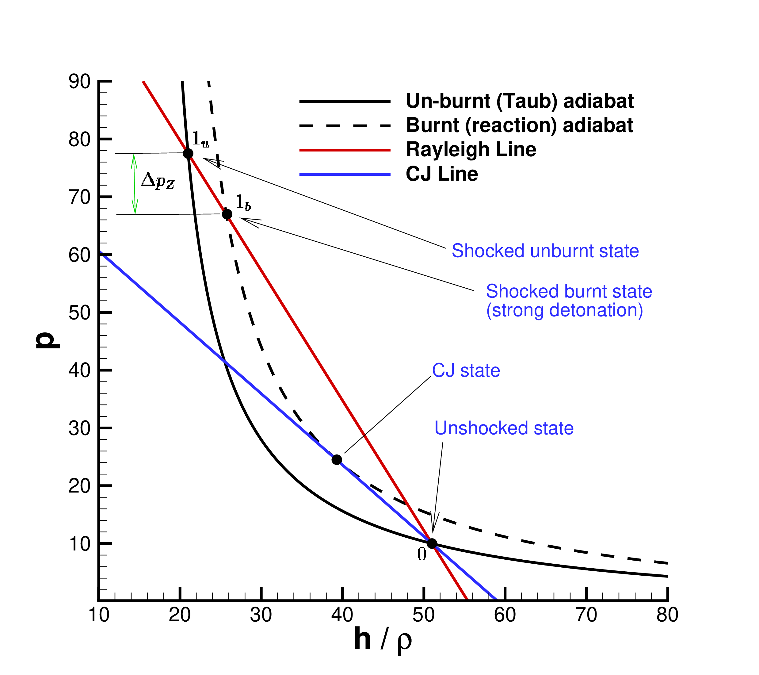
Since the first three equations of the system 10 –13 do not have any source term, the standard Rankine Hugoniot conditions for un-reactive flows apply unmodified (see [43], Sect. 4.4.3), i.e. \[\begin{align} \llbracket \rho \gamma_w w \rrbracket&=0, \tag{15}\\ \llbracket h\rho \gamma_w^2 w^2+p \rrbracket&=0, \tag{16}\\ \llbracket h\rho \gamma_w^2 w \rrbracket&=0\,,\tag{17} \end{align}\] where, as usual, \(\llbracket x \rrbracket=x_1-x_0\) indicates the difference of the variable \(x\) across the two sides of the shock3. From (15 ) the mass flux \(m=-\gamma_w \rho w>0\) is constant through the shock front. By substituting the mass flux in (16 ) and (17 ), they are equivalent to: \[\begin{align} \llbracket p\rrbracket&= -m^2 \bigg\llbracket \frac{h}{\rho} \bigg\rrbracket, \tag{18}\\ \llbracket h \gamma_w \rrbracket&=0.\tag{19}\\ \llbracket h^2 \rrbracket&=\left(\frac{h_0}{\rho_0}+\frac{h_1}{\rho_1}\right)\llbracket p\rrbracket\,.\tag{20} \end{align}\] In the presence of combustion, all relations from 15 to 20 still hold, with the reaction energy affecting the thermodynamics through the specific enthalpy \(h\). The whole process can be represented in the \((h/\rho,p)\) plane, as shown in Fig. 1, which is the relativistic analog of the \((1/\rho,p\)) plane in the classical (Newtonian) case [45], [46]. All the points in this plane have a enthalpy that can be written as a function of the pressure after solving the quadratic equation \[\label{eq:reaction95adiabat} \frac{p+p_0(\Gamma-1)}{\Gamma p}h^2+\frac{\Gamma-1}{\Gamma}(1+qZ)\frac{p-p_0}{p}h-h_0^2-\frac{h_0}{\rho_0}(p-p_0)=0\,,\tag{21}\] which follows from Eq. 20 by replacing the mass density \(\rho\) via the equation of state 2 . See also Eq. (4.16) of [47] for a similar expression without the combustion term \(qZ\). For each value of \(Z\), Eq. 21 generates a curve in the \((h/\rho,p)\) plane, and in Fig. 1 the two extreme cases are drawn. Firstly, the solid line indicates those states that can be connected through a shock to the initial "\(0\)" state, but for which combustion has not been ignited yet, hence with \(Z=1\). They collectively form the so called inert Taub adiabat, after [48]. In the figure, a representative of such state is indicated by "\(1_u\)", with the subscript \(u\) specifying that it is an un-burnt state. Secondly, the dashed line indicates those states that can be connected through a shock to the initial "\(0\)" state, but for which complete combustion has occurred, hence with \(Z=0\). In the figure, a representative such state is indicated by "\(1_b\)", with the subscript \(b\) specifying that it is completely burnt state. The two states "\(1_u\)" and "\(1_b\)" belong to the same Reyleigh line, which comes from Eq. 18 for a constant mass flux \(m\).
In the figure we have also reported the so called Chapman-Jouguet (CJ) line, which is tangent to the fully burnt adiabat. We recall that, both in the Newtonian and in the relativistic regime, the CJ line corresponds to the minimum possible mass flux through the detonation wave [9]. The computation of the CJ state, including the value of the mass flux \(m_{CJ}\), is postponed to Sect. 2.4.
2.3 The relativistic Zel’dovich-von Neumann-Doering profile↩︎
Ahead of the shock, which moves at constant speed \(V_s\), no reaction has occurred yet. Just behind the shock front, the temperature raises abruptly, igniting the reaction. This is the state "\(1_u\)". As the combustion goes on, new shocked states all along the Reyleigh line are formed, up until the final fully burnt shocked state "\(1_b\)" is produced. In this way a Zel’dovich-von Neumann-Doering (ZND) profile, characterized by a typical spike (henceforth denoted as the Zel’dovich spike), is produced.
Let us see how this Zel’dovich profile can be computed in semi-analytic way. First of all, from (15 ) we find the following additional useful kinematic expressions: \[\begin{align} w(\rho,m) &=-\frac{m}{\sqrt{m^2+\rho^2}} \tag{22}\\ \gamma_w(\rho,m) &=\frac{\sqrt{m^2+\rho^2}}{\rho}\tag{23}\\ v(\rho,m) &=\frac{V_{s}\sqrt{m^2+\rho^2}-m}{\sqrt{m^2+\rho^2}-V_{s}m} \tag{24}\,. \end{align}\] We now perform a Lorentz transformation into the rest frame of the shock front, i.e. \[\label{eq:lorentz} \xi = \gamma_s( x-V_{s} t)\,, \textrm{where}\gamma_s=\frac{1}{\sqrt{1-V_s^2}}\tag{25}\] and we reduce Eq. 7 into an ordinary differential equation (ODE) \[\partial_{\xi}Z = \frac{K(T) Z}{\gamma\gamma_s(V_s-v)}=\frac{\rho K(T) Z}{m} \,, \label{eq:odez}\tag{26}\] where we have used \(\partial_t=-V_s\gamma_s\partial_\xi\) and \(\partial_x=\gamma_s\partial_\xi\) and where the mass flux has been written as \[m=-\gamma_w \rho w=\rho \gamma\gamma_s(V_s-v)\,.\] Let \(V_0=(\rho_0,v_0,p_0,Z_0)\) be the vector of primitive variables of the unshocked (and unburnt) state with \(Z_0=1\). From (15 ) we compute the mass flux as \(m=-\gamma_{w,0} \rho_0 w_0\). According to (19 ), \(L= h_0 \gamma_{w,0}\) is constant through the shock, thus leading to \[\label{eq:h-rho} h(\rho)=\frac{L}{\gamma_w}=\frac{L \rho}{\sqrt{m^2 +\rho^2}}\,.\tag{27}\] Moreover, from the Rankine Hugoniot condition (18 ) we can also write: \[p(\rho)=p_0 -m^2 \left( \frac{L }{\sqrt{m^2 +\rho^2}}- \frac{h_0}{\rho_0}\right). \label{eq:prho}\tag{28}\] We now replace the pressure \(p\) by the equation of state 2 , to find \[\begin{align} \frac{\Gamma-1}{\Gamma}\rho(h-1-qZ) &=&p_0 -m^2 \left( \frac{L }{\sqrt{m^2 +\rho^2}}- \frac{h_0}{\rho_0}\right)\\ \Longrightarrow \frac{\Gamma-1}{\Gamma}\rho\left(\frac{L \rho}{\sqrt{m^2 +\rho^2}}-1-qZ\right) &=&p_0 -m^2 \left( \frac{L }{\sqrt{m^2 +\rho^2}}- \frac{h_0}{\rho_0}\right). \label{rhoZ} \end{align}\tag{29}\] This leads to a fourth degree polynomial equation of the type \[\label{eq:rho4} a\rho^4 +b\rho^3 +c \rho^2 +d \rho +e=0\,,\tag{30}\] with coefficients that depend only on the state ahead of the shock and on the value of \(Z\) as follow: \[\begin{align} \tag{31} a &= \left( \frac{\Gamma - 1}{\Gamma} \right)^{2} \left( L^{2} - (1 + qZ)^{2} \right) \\[8pt] b &= -2 \left( \frac{\Gamma - 1}{\Gamma} \right) (1 + qZ)\left( p_{0} + m^{2}\frac{h_{0}}{\rho_{0}} \right) \\[8pt] c &= -\left( p_{0} + m^{2}\frac{h_{0}}{\rho_{0}} \right)^{2} + \left( \frac{\Gamma - 1}{\Gamma} \right) m^{2} \left( 2L^{2} - \left( \frac{\Gamma - 1}{\Gamma} \right)(1 + qZ)^{2} \right) \\[8pt] d &= -2 \left( \frac{\Gamma - 1}{\Gamma} \right) (1 + qZ)\left( p_{0} + m^{2}\frac{h_{0}}{\rho_{0}} \right) m^{2} \\[8pt] \tag{32} e &= m^{2}\left( m^{2}L^{2} - \left( p_{0} + m^{2}\frac{h_{0}}{\rho_{0}} \right)^{2} \right)\,. \end{align}\] The strategy is now the following: we solve numerically the ODE of Eq. 26 using a standard fourth order Runge-Kutta scheme, where the coefficients 31 –32 of the quartic for the computation of \(\rho\) on the right hand side of 26 depend themselves on \(Z\). For each value of \(Z\) that is obtained from that ODE, we solve the quartic 30 to obtain \(\rho(Z)\), and, subsequently, \(p(Z)\) and \(v(Z)\) from (28 ) and (24 ). In this way the whole ZND profile can be computed.
2.4 The Chapman-Jouguet state↩︎
Unlike the Newtonian case, a closed form expression for the Chapman-Jouguet state is not available in the relativistic regime. As discussed above when commenting Fig.1, the mass flux \(m_{CJ}\) is obtained as the slope of the line that is tangent to the Taub adiabat and passes trough the initial unburnt state. The numerical computation of the CJ state that we propose here is based on the strategy outlined in [49]. We first use Eq. (20 ) to build the functional \[\mathcal{H}:= h^2 -h_0^2 -\left(\frac{h}{\rho}+\frac{h_0}{\rho_0}\right)(p-p_0).\] The curve \(\mathcal{H}=0\) describes the Hugoniot curve in the \(\left(\frac{h}{\rho},p\right)\) plane. Its total differential is given by \[\begin{align} d{\mathcal{H}}&= 2h d{h} -(p-p_0) d{\left(\frac{h}{\rho}\right)}-\left(\frac{h}{\rho}+\frac{h_0}{\rho_0}\right) d{p},\nonumber \\ &=2hT d{s} -(p-p_0) d{\left(\frac{h}{\rho}\right)}+\left(\frac{h}{\rho}-\frac{h_0}{\rho_0}\right) d{p}\,, \label{dH1} \end{align}\tag{33}\] where we have used the first principle of thermodynamics in the form \[\begin{align} \tag{34} d{h} &= \frac{1}{\rho} d{p} + Td{s},\\ d{\epsilon} &= T d{s} +\frac{p}{\rho^2} d{\rho} \tag{35}\,. \end{align}\] From these we deduce \[\begin{align} \tag{36} \left. \frac{\partial h }{\partial p} \right|_{s}&=\frac{1}{\rho}, \qquad \qquad \qquad \qquad \left. \frac{\partial h }{\partial s} \right|_{p}=T,\\ \tag{37} \left. \frac{\partial \epsilon }{\partial \rho} \right|_{s}&=\frac{p}{\rho^2}=c_v \left. \frac{\partial T }{\partial \rho} \right|_{s}, \qquad \left. \frac{\partial \epsilon }{\partial s} \right|_{p}=T+ \frac{p}{\rho^2} \left. \frac{\partial \rho }{\partial s} \right|_{p}\,. \end{align}\] After introducing \(\tau=h/\rho\) for ease of notation, the Rankine Hugoniot condition (18 ) becomes \(\llbracket p\rrbracket / \big\llbracket \tau \big\rrbracket= -m^2\), which, in differential form, translates into \(dp=-m^2 d\tau\). Using \((p,\tau)\) as primary thermodynamic variables, we can write \[\label{dsdtau} \frac{ds}{d\tau}= \left. \frac{\partial s}{\partial \tau} \right|_{p}+ \left. \frac{\partial s}{\partial p} \right|_{\tau} \frac{dp}{d\tau}\,.\tag{38}\] Moreover, from the differential relation \(d\tau=\partial\tau/\partial p|_s dp + \partial\tau/\partial s|_p ds\) it follows that \[\label{dsdp} \left. \frac{\partial s}{\partial p} \right|_{\tau} = -\bigg( \left. \frac{\partial \tau}{\partial s} \bigg)\right|_{p}^{-1} \left. \frac{\partial \tau }{\partial p} \right|_{s}\,.\tag{39}\] Since the Chapman-Jouguet state is characterized by \(\frac{d\mathcal{H}}{d\tau}=0\) and \(dp/d\tau=(p-p_0)/(\tau-\tau_0)\), we can write, from Eq. 33 \[\begin{align} \frac{d\mathcal{H}}{d\tau}=&2hT\bigg( \left. \frac{\partial \tau}{\partial s} \bigg)\right|_{p}^{-1} + \bigg( 2hT \bigg( \left. \frac{\partial \tau}{\partial s} \bigg)\right|_{p}^{-1} \left. \frac{\partial \tau }{\partial p} \right|_{s} + (\tau-\tau_0) \bigg)\frac{dp}{d\tau} -(p-p_0)=0\nonumber\\ \Longrightarrow &2hT\bigg( \left. \frac{\partial \tau}{\partial s} \bigg)\right|_{p}^{-1} + 2hT \bigg( \left. \frac{\partial \tau}{\partial s} \bigg)\right|_{p}^{-1} \left. \frac{\partial \tau }{\partial p} \right|_{s} \frac{dp}{d\tau}=0\,, \label{dHdtau} \end{align}\tag{40}\] where we have used both 38 and 39 . From (36 ) it follows immediately that: \[\begin{align} \tag{41} \left. \frac{\partial \tau }{\partial p} \right|_{s} &= \frac{1}{\rho}\left. \frac{\partial h }{\partial p} \right|_{s}-\frac{h}{\rho^2} \left. \frac{\partial \rho }{\partial p} \right|_{s} =\frac{1}{\rho^2}-\frac{h}{\rho^2} \left. \frac{\partial \rho }{\partial p} \right|_{s} \\ \tag{42} \left. \frac{\partial \tau}{\partial s} \right|_{p}&= \frac{1}{\rho} \left. \frac{\partial h}{\partial s} \right|_{p}- \frac{h}{\rho^2}\left. \frac{\partial \rho}{\partial s} \right|_{p}=\frac{p}{\rho^2}- \frac{h}{\rho^2}\left. \frac{\partial \rho}{\partial s} \right|_{p}\,. \end{align}\] So far, no assumption has been made on the equation of state adopted. If we now specialize to an ideal gas equation of state, i.e. Eq. 3 in (37 ) we find that: \[\left. \frac{\partial \rho }{\partial p} \right|_{s} =\frac{\rho}{\Gamma p},\qquad \left. \frac{\partial \rho}{\partial s} \right|_{p}=-\frac{\rho(\Gamma-1)}{\Gamma },\] Thus Eq. 41 42 become \[\begin{align} \tag{43} \left. \frac{\partial \tau }{\partial p} \right|_{s} &= \frac{1}{\rho^2}- \frac{\tau}{\Gamma p},\\ \tag{44} \left. \frac{\partial \tau}{\partial s} \right|_{p}&=\frac{p}{\rho^2}+\frac{\tau(\Gamma-1)}{\Gamma }, \end{align}\] Replacing 43 –44 into Eq. (40 ) we obtain the relation: \[\left.\frac{dp}{d\tau}\right|_{CJ}=-m_{CJ}^2=\frac{ \Gamma p\rho^2 }{p \Gamma - h\rho}. \label{eqCJ}\tag{45}\] For any initial state \((\rho_0,v_0,p_0,Z_0=1)\) we solve numerically a system of three equations in three unknowns, namely: Eq. (18 ), Eq. (30 ) and Eq. (45 ), to find \(\rho\), \(p\) and the mass flux \(m\) at the Chapman-Jouguet state. Wherever the enthalpy \(h\) is needed, this is obtained from (2 ), while at the CJ state Z is zero and the constant \(L\), that is needed for the coefficients of the quartic equation 30 , follows from Eq. 27 , i.e. \[L=L(m)=\frac{h_0}{\rho_0}\sqrt{m^2+\rho_0^2}\,.\]
| \(q\) | \(m_{CJ}\) | \(\rho_{CJ}\) | \(p_{CJ}\) |
|---|---|---|---|
| 0.001 | \(0.698452\) | \(1.0060743\) | \(10.081408\) |
| 0.01 | \(0.707656\) | \(1.0192469\) | \(10.285730\) |
| 0.1 | \(0.737000\) | \(1.0611998\) | \(10.860056\) |
| 0.5 | \(0.790686\) | \(1.1377871\) | \(12.073315\) |
| 0.8 | \(0.816556\) | \(1.1746128\) | \(12.718200\) |
Following this procedure, it is possible to compute the variables of the CJ state for any set of the initial states "0". Table 1 reports the CJ variables in a representative case, for different values of the parameter \(q\).
2.5 A new relativistic effect↩︎
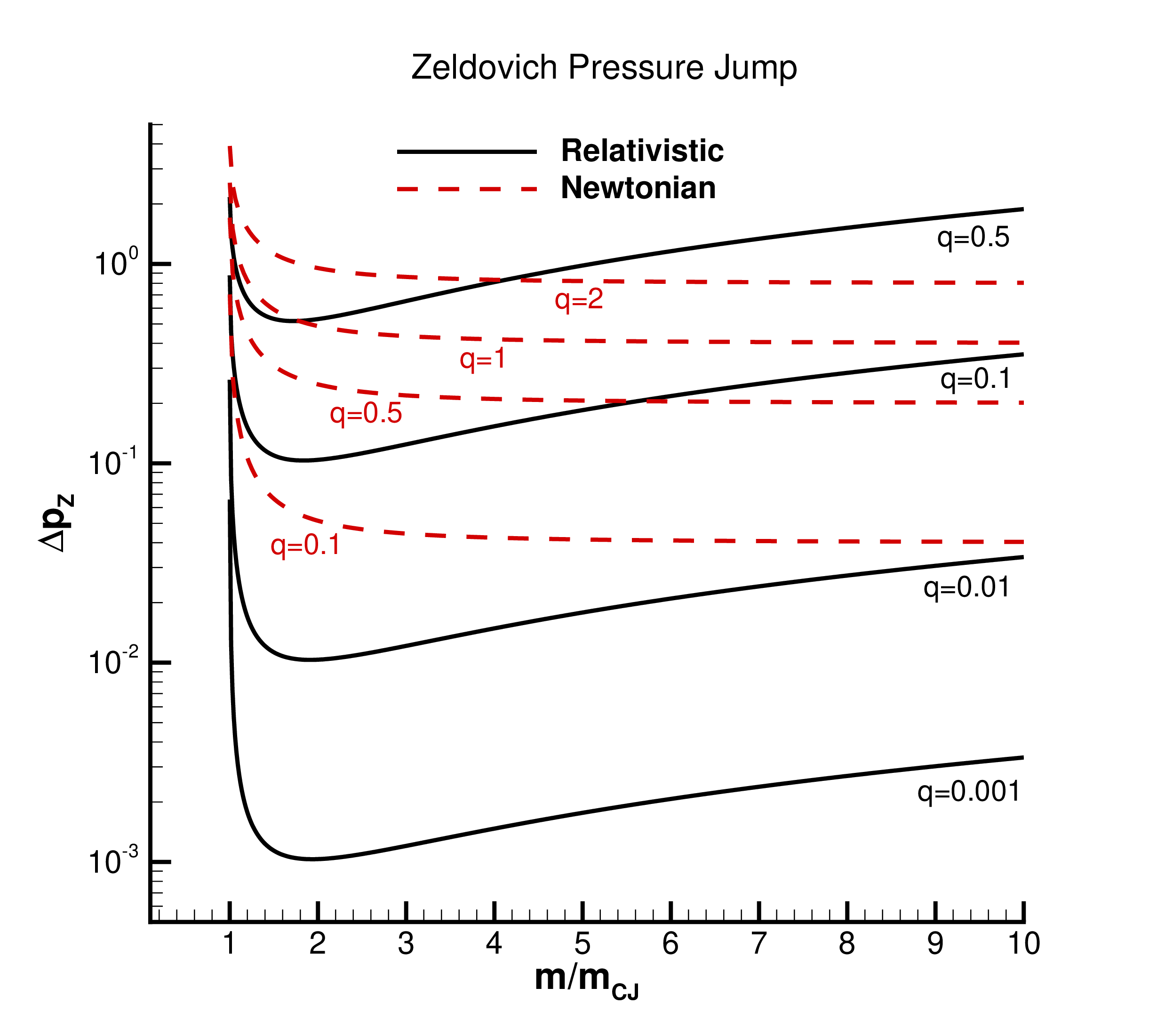
Qualitatively, the phenomenology described so far does not differ much from what was already known in the classical (Newtonian) context. Fig. 4 of [3], for instance, analyzes classical detonations reproducing the same physical effects as those shown in Fig. 1 above, except for the quantities reported along the axis, which in the relativistic case are \((h/\rho,p)\) rather than \((1/\rho,p)\). However, there is a purely relativistic effect hidden in those figures which is related to the Zel’dovich pressure jump \(\Delta p_Z\). This quantity is highlighted in Fig. 1 with a green arrowed vertical line. It represents the pressure difference among the shocked un-burnt and the shocked fully burnt states connected by the Rayleigh line. Now, the following crucial difference is observed:
Newtonian regime: the Zel’dovich pressure jump is maximum at the Chapman-Jouguet state, which, we recall, corresponds to the minimum possible mass flux. When the mass flux through the shock front is increased, the Zel’dovich pressure jump decreases monotonically to the asymptotic value \(\Delta p_Z=(\Gamma-1)q\rho_0\).
Relativistic regime: the Zel’dovich pressure jump \(\Delta p_Z\) decreases for small mass fluxes, down to a minimum value, but then increases again to arbitrary large values for very high mass fluxes. Hence, in the extreme relativistic regime, the Zel’dovich pressure jump can become huge.
The comparison among the two regimes is reported in Fig. 2 for a few generic but representative thermodynamic states. The continuous black lines and the dashed red lines refer to the relativistic and to the Newtonian regimes, respectively. While in both cases the Zel’dovich pressure jump increases with \(q\), the dependence on the mass flux is quite different, as just commented. The comparison has been performed after adopting the same values of the unshocked state, i.e. \(p_0=10\), \(v_0=0\), \(\rho_0=1\), but different adiabatic indices, i.e. \(\gamma=4/3\) and \(\gamma=1.4\), for the relativistic and for the Newtonian regimes, respectively. Since the units of measure are effectively different in the two regimes, absolute numbers are not relevant in this plot, but one should only pay attention to the different functional dependence on the mass flux.
This purely relativistic effect, which has no analog in the Newtonian case, has also an impact on the energy that is released during the combustion, which can be computed as \[\begin{align} \Delta E_{comb,rel} &=&q_0\cdot M_{burnt}=q_0\cdot\int \rho\gamma Z d\xi \,,\\ \Delta E_{comb,Newt}&=&q_0\cdot M_{burnt}=q_0\cdot\int \rho Z d\xi\,, \end{align}\] with integration performed along the ZND profile.
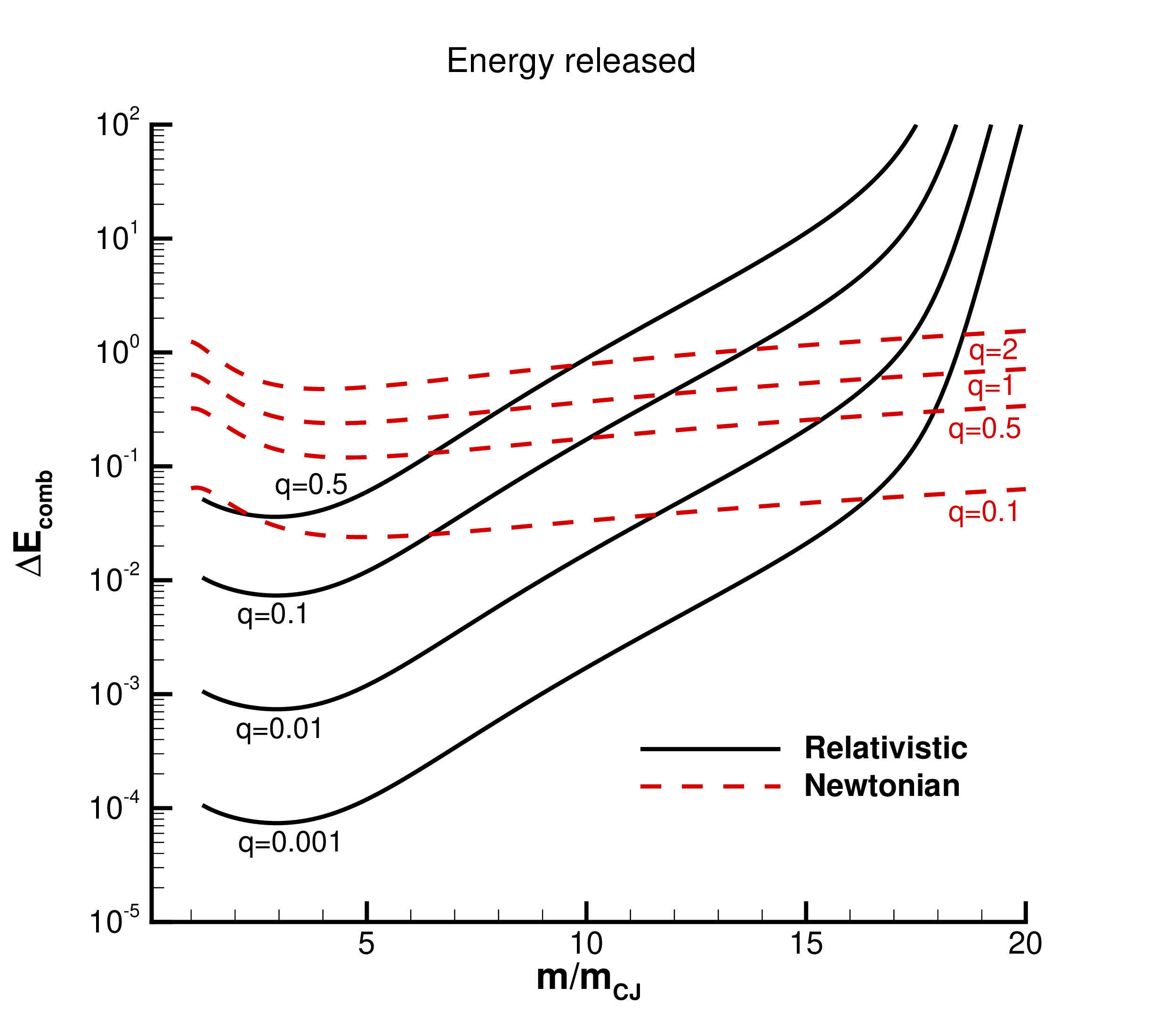
The result of this comparison is shown in Fig. 3. While the Zel’dovich pressure jump of Fig. 2 does not depend on the reaction rate \(K(T)\), the amount of energy released is indeed affected by \(K(T)\), for which we have assumed the Arrhenius model, adopting \(E_a=35\) and \(K_0=120\). There are at least two results that can be extracted from the analysis reported in Fig. 3. The first one is that, for small values of the mass flux, say \(m\sim\) a few \(m_{CJ}\), the energy manifests a mild decreasing behavior, which is due to the reduction of the Zel’dovich pressure jump, that is present both in the Newotonian and in the relativistic regime. The second result is that, for large mass fluxes, the higher mass densities of the shocked detonation play a major role. In the Newtonian regime, such higher densities contrast the asymptotic reduction of the Zel’dovich pressure jump, producing a linear growth of the energy released as the mass flux grows. In the relativistic regime, the higher mass densities combine with the increasing values of the Zel’dovich pressure jump, producing an exponential growth of the energy released. This enhanced efficiency of energy production in highly relativistic strong detonations can become important in the astrophysical context, and it may deserve a separate investigation.
3 The numerical method↩︎
3.1 ALE finite volume schemes↩︎
In this section we will briefly recall the strategy to solve stiff hyperbolic balance laws through high order accurate Arbitrary Lagrangian-Eulerian one-step TVD finite volume schemes. The state vector is the typical one for special relativistic hydrodynamics, with the addition of the combustion term, i.e. \(\mathbf{Q}=(D,S,E,W)\), with \(W=\rho\gamma Z = D \, Z\). Moreover, fluxes and sources are defined by \(\mathbf{F}(\mathbf{Q})=(Dv, Sv +p, S, W v)\) and \(\mathbf{S}(\mathbf{Q})=(0,0,0,-K(T)\rho Z)\). In this way, the one dimensional PDEs 10 13 can be cast as a nonlinear system of balance laws \[\frac{\partial \mathbf{Q}}{\partial t} +\frac{\partial \mathbf{F}(\mathbf{Q})}{\partial x} = \mathbf{S}(\mathbf{Q})\label{balancelaw}\tag{46}\] defined within a spatial domain \(\Omega(t)\) that moves and changes in time. Our aim is to follow the fluid as the shock propagates, hence with a mesh that moves with the speed of the shock. The computational domain \(\Omega\) is discretized by a set of moving mesh points \(x_{i+1/2}\) that move with a general mesh velocity \(V_{i+1/2}\), thus: \[\frac{d}{dt}x_{i+1/2}=V_{i+1/2}.\] The spacial control volumes are defined at the current time \(t^n\) as \(T^n=[x_{i-1/2}^n, x_{i+1/2}^n]\) where \(x_{i+1/2}^n=x_{i+1/2}(t^n)\). We obtain the integral formulation for the balance law (46 ) by integrating it in the moving space-time control volume \([x_{i-1/2}(t), x_{i+1/2}(t)]\times[t^n, t^{n+1}]\) and by applying the Gauss Theorem: \[\label{eq:generalALEscheme} \Delta x^{n+1}_i \mathbf{Q}^{n+1}_i = \Delta x^n_i \mathbf{Q}^n_i - \Delta t \left( \mathbf{F}^V_{i+\frac{1}{2}} - \mathbf{F}^V_{i-\frac{1}{2}} \right) + \Delta x_i^n \, \Delta t \, \mathbf{S}_i.\tag{47}\] We denoted the time step \(\Delta t =t^{n+1}-t^n\), while the mesh spacing at time \(t^n\), \(\Delta x^n_i=x_{i+1/2}^n-x_{i-1/2}^n\). As in standard finite volume schemes, the cell average at time \(t^n\), the fluxes and the sources are respectively given by \[\begin{align} \mathbf{Q}^n_i &=& \frac{1}{\Delta x^n_i} \int_{x^n_{i-\frac{1}{2}}}^{x^n_{i+\frac{1}{2}}} \mathbf{Q}(x, t^n) dx\,,\\ \mathbf{F}^V_{i+\frac{1}{2}} &=& \frac{1}{\Delta t} \int_{t^n}^{t^{n+1}} \left[ \mathbf{F}(x_{i+\frac{1}{2}}(t), t) - V_{i+\frac{1}{2}}(t) \, \mathbf{Q}(x_{i+\frac{1}{2}}(t), t) \right] dt\,,\\ \mathbf{S}_i &=& \frac{1}{\Delta x^n_i \, \Delta t} \int_{t^n}^{t^{n+1}} \int_{x_{i-\frac{1}{2}}(t)}^{x_{i+\frac{1}{2}}(t)} \mathbf{S}(\mathbf{Q}(x,t)) dx \, dt\,. \end{align}\] The exact flux \(\mathbf{F}^V_{i+1/2}\) is approximated with a numerical flux \(\mathbf{F}^V(\mathbf{Q}^-_h, \mathbf{Q}^+_h)\) where \(\mathbf{Q}^-_h=\mathbf{Q}(x_{i+1/2}^-, t)\) and \(\mathbf{Q}^+_h=\mathbf{Q}_h(x_{i+1/2}^+, t)\) and: \[\mathbf{F}^V(\mathbf{Q},V)=\mathbf{F}(\mathbf{Q})-V\mathbf{Q}\;\;\;\;\;\;\;and \;\;\;\;\;\;\;{\boldsymbol{A}}^V(\mathbf{Q},V)=\frac{\partial \mathbf{F}^V}{\partial \mathbf{Q}}.\] Second-order accuracy in space is achieved through a Total Variation Diminishing (TVD) spatial reconstruction using as \(\mathbf{Q}_h^+= \mathbf{Q}^{n+\frac{1}{2},\,+}_{i+\frac{1}{2}}\) and \(\mathbf{Q}_h^-= \mathbf{Q}^{n+\frac{1}{2},\,-}_{i+\frac{1}{2}}\) the following reconstruction: \[\mathbf{Q}^{n+\frac{1}{2},\,\mp}_{i\pm\frac{1}{2}} = \mathbf{Q}^n_i \pm \frac{1}{2}\,\Delta \mathbf{Q}_i + \frac{1}{2}\, \Delta t \,\partial_t \mathbf{Q}_i,\] where: \[\begin{align} \partial_t \mathbf{Q}_i &\approx - \frac{ \mathbf{F}^V\left(\mathbf{Q}^{n,-}_{i+\frac{1}{2}}\right) - \mathbf{F}^V\left(\mathbf{Q}^{n,+}_{i-\frac{1}{2}}\right) }{\Delta x}. \\ \Delta \mathbf{Q}_i &= \operatorname{minmod} \bigl( \mathbf{Q}^n_{i+1} - \mathbf{Q}^n_i,\; \mathbf{Q}^n_i - \mathbf{Q}^n_{i-1} \bigr), \\ \mathbf{Q}^{n,\,\mp}_{i\pm\frac{1}{2}} &= Q^n_i \pm \frac{1}{2}\,\Delta \mathbf{Q}_i. \end{align}\]
In our numerical tests we have computed these fluxes following two different approaches
Rusanov flux: \[\mathbf{F}^{V}_h(\mathbf{Q}_h^-,\mathbf{Q}_h^+)=\frac{1}{2}\left(\mathbf{F}^V (\mathbf{Q}_h^-,V_{1+\frac{1}{2}})+ \mathbf{F}^V(\mathbf{Q}_h^+,V_{1+\frac{1}{2}})\right) -\frac{1}{2}s_{max}(\mathbf{Q}_h^+-\mathbf{Q}_h^-)\] where \(s_{\max}=\max\bigl(\max(|\lambda({\boldsymbol{A}}^V(\mathbf{Q}_h^-,V_{i+\frac{1}{2}}))|),\max(|\lambda({\boldsymbol{A}}^V(\mathbf{Q}_h^+,V_{i+\frac{1}{2}}))|)\bigr)\) is the maximum signal speed,
the Osher-type flux [50]: \[\begin{align} \mathbf{F}^V_h(\mathbf{Q}^-_h, \mathbf{Q}^+_h) =\;\frac{1}{2} \left[ \mathbf{F}^V(\mathbf{Q}^-, V_{i+\frac{1}{2}}) + \mathbf{F}^V(\mathbf{Q}^+, V_{i+\frac{1}{2}}) \right] - \frac{1}{2} \left( \int_0^1 \left| {\boldsymbol{A}}^V(\boldsymbol{\psi}(s), V_{i+\frac{1}{2}}) \right| ds \right)(\mathbf{Q}^+_h - \mathbf{Q}^-_h)\,, \end{align}\] where \(\boldsymbol{\psi}(s)\) is a straight line segment path connecting the two states \(\mathbf{Q}^-_h\) and \(\mathbf{Q}^+_h\), i.e. \[\boldsymbol{\psi} = \boldsymbol{\psi}(\mathbf{Q}_h^-, \mathbf{Q}_h^+, s) = \mathbf{Q}_h^- + s \left( \mathbf{Q}_h^+ - \mathbf{Q}_h^- \right), \qquad 0 \leq s \leq 1\,.\] The absolute value of a matrix is calulated by: \[|{\boldsymbol{A}}|=\mathbf{R}|\Lambda|\mathbf{R}^{-1}\] with \(\mathbf{R}\) the matrix of the right-eigenvectors and \(|\Lambda|\) the diagonal matrix of the absolute values of the eigenvalues of \({\boldsymbol{A}}\).
In our specific case, since the mesh velocity is constant in space and in time, the new position of the mesh point \(x_{i+1/2}\) at time \(t^{n+1}\) is simply given by \(x_{i+1/2}^{n+1}=x_{i+1/2}^{n}+ \Delta t V\).
3.2 Conversion from conserved to primitive variables↩︎
In order to compute both the fluxes \(\mathbf{F}\) and the sources \(\mathbf{S}\), given a state vector of conserved variables \(\mathbf{Q}\), it is
necessary to recover the primitive variables \(\rho, v, p\) and \(Z\). Except for \(Z\), which can be easily computed as \(Z=W/D\), the remaining quantities cannot be explicitly reformulated using conservative variables, a fact that represents a well known obstacle in relativistic hydrodynamics, with a variety of solutions proposed over the years
[43], [51]–[53]. Here we follow the same approach of [54], which has been proved to be very robust in the absence of
reactions. First of all, we define the space of admissible solutions: \[\mathcal{G}=\left\{ \mathbf{Q}=(D,S,E,W)\; | \;\rho(\mathbf{Q})>0,\; p(\mathbf{Q})>0,\; |v(\mathbf{Q})|<1,\; Z(\mathbf{Q})\in[0,1]
\right\}.\] If \(p(\mathbf{Q})\) is known then: \[\begin{align}
\tag{48} v(\mathbf{Q}) &=& \frac{S}{E + p(\mathbf{Q})}, \\
\tag{49} \rho(\mathbf{Q}) &=& D\,\sqrt{1 - v^2(\mathbf{Q})} .
\end{align}\] Similarly to [55] we now
demonstrate that the admissible set \(\mathcal{G}\) is equivalent to the following set \[\mathcal{G}_1=\left\{ \mathbf{Q}=(D,S,E,W)\; | \;D>0,\;g(\mathbf{Q}):=E-\sqrt{D^2(1+qZ)^2 +S^2}>0,
\;\; W/D\in[0,1] \right\},\] Let us first verify that \(\mathcal{G}\subseteq \mathcal{G}_1\), namely that if \(\mathbf{Q}\in \mathcal{G}\) then \(\mathbf{Q}\in \mathcal{G}_1\).
First of all, \(D=\rho \gamma = \frac{\rho}{\sqrt{1-v^2}}>0\) and \(E=\frac{\rho h}{1-v^2}-p>e>0\) if \(\mathbf{Q}\in \mathcal{G}\) . As previously
mentioned, \(W/D=Z\) so \(Z\in[0,1]\) if and only if \(W/D\in[0,1]\). We now only need to verify that \(E>\sqrt{D^2(1+qZ)^2
+S^2}\) which is true if and only if \(E^{2} > \left(D^{2} (1+qZ)^2 +S^2\right)\). Now, it follows that \[\begin{align} E^{2} - \left(D^{2}(1+qZ)^2 +S^2\right) &= \left(\frac{\rho
h}{1 - v^{2}} - p\right)^{2} - \frac{\rho^{2}}{1 - v^{2}}(1+qZ)^2 - \left(\frac{\rho h v}{1 - v^{2}}\right)^{2} \nonumber\\[6pt] &= \left(\frac{\rho h}{1 - v^{2}}\right)^{2} + p^{2} - 2p \frac{\rho h}{1 - v^{2}} - \frac{\rho^{2}}{1 - v^{2}}(1+qZ)^2 -
\left(\frac{\rho h v}{1 - v^{2}}\right)^{2} \nonumber\\[6pt] &= \frac{1}{1 - v^{2}} \left[ (\rho h - p)^{2} - \rho^{2}(1+qZ)^2 - p^{2} v^{2} \right] \nonumber \\[6pt] &\overset{(\ref{phrelation-1})}{=} \frac{1}{1 - v^{2}} \left[
\rho^{2}\left(1+\frac{1}{\Gamma-1}\frac{p}{\rho}+q Z\right)^{2} - \rho^{2}(1+qZ)^2 - p^{2} v^{2} \right]\nonumber\\[6pt] &= \frac{1}{1 - v^{2}} \left[\frac{1}{(\Gamma-1)^2}p^2+\frac{2}{\Gamma-1}\rho p(1+qZ) - p^{2} v^{2} \right] \nonumber\\[6pt]
&\overset{|v|<1}{>} \frac{1}{1 - v^{2}} \left[ p^2 \frac{\Gamma(2-\Gamma)}{(\Gamma-1)^2}+ \frac{2}{\Gamma-1}\rho p(1+qZ) \right] > 0
\end{align}\] for any \(\mathbf{Q}\in\mathcal{G}\) and \(\Gamma\in (1,2]\). Thus \(q(\mathbf{Q})>0\) and \(\mathbf{Q}\in
\mathcal{G}_1\).
Secondly, let us verify that \(\mathcal{G}_1\subseteq \mathcal{G}\), namely that if \(\mathbf{Q}\in \mathcal{G}_1\) then \(\mathbf{Q}\in \mathcal{G}\).
Consider the function of \(p\) defined by \[\label{phipprim2cons} \Phi(p) := \frac{S^{2}}{E+p} + D(1+qZ) \sqrt{1 - \frac{S^{2}}{(E+p)^{2}}}
+\frac{p}{\Gamma -1} - E , \qquad p \in [0,+\infty),\tag{50}\] with \(\mathbf{Q}\in \mathcal{G}_1\). Obviously, \(\Phi(p) \in C^{1}[0,+\infty)\), and \[\Phi'(p) = -\frac{S^2}{(E+p)^2}\left(1-\frac{D(1+qZ)}{\sqrt{(E+p)^2-S^2}}\right) +\frac{1}{\Gamma-1} \ge 1 -\frac{S^2}{(E+p)^2} > 0,\] for all \(p \in [0,+\infty)\), when \(E>\sqrt{D^{2}(1+qZ)^2+S^{2}}\) and \(\Gamma \in (1,2]\) since \(Z=W/D \in[0,1]\). This means that \(\Phi(p)\) is a strictly
monotonically increasing function of \(p\) on \([0,+\infty)\). Since \[\begin{align} \Phi(0) &= \frac{S^{2}}{E} + D (1+qZ)\sqrt{1 - \frac{S^{2}}{E^{2}}} - E
\nonumber\\ &= \left( D (1+qZ) -\sqrt{E^2-S^2} \right)\sqrt{\frac{E^2-S^2}{E^2}} < 0,
\end{align}\] and \[\lim_{p \to +\infty} \Phi(p) = +\infty, \qquad \text{since } \lim_{p \to +\infty} \frac{\Phi(p)}{p} = \frac{1}{\Gamma-1} > 0 ,\] by the intermediate value theorem and the monotonicity of \(\Phi(p)\), there exists a unique positive solution to the equation \(\Phi(p)=0\) and such \(p(\mathbf{Q})\) is also the solution of: \[E+p=D(1+qZ)\gamma +\frac{\Gamma}{\Gamma-1}p\gamma^2\,.\] It is immediate that for any \(\mathbf{Q}\in \mathcal{G}_1\) and \(p(\mathbf{Q})\) the solution of (50 ) \[v(\mathbf{Q}) = \frac{S}{E+p(\mathbf{Q})} < \frac{S}{E} < 1, \qquad \rho(S) = \frac{D}{\sqrt{1-v^{2}(\mathbf{Q})}} > 0\,,\] which concludes the proof.
Another easily proven property of the set \(G_1\) is that it is convex. Following closely the argument of [55], we verify that
for any \(\mathbf{Q}_1,\;\mathbf{Q}_2 \in \mathcal{G}_1\) also \(\mathbf{Q}_{\lambda}:=\lambda \mathbf{Q}_1 + (1-\lambda)\mathbf{Q}_2\in \mathcal{G}_1\) for any \(\lambda\in[0,1]\).
Since \(D_1,\;D_2 \in \mathcal{G}_1\) then \(D_{\lambda}:=\lambda D_1+(1-\lambda) D_2>0\). Similarly follows that \(W_{\lambda}:=\lambda W_1+(1-\lambda)
W_2\geq0\). Let us now verify that \(W_{\lambda}/D_{\lambda}\leq 1\), this is equivalent to verify that: \[\label{convexityW} \lambda
(W_1-D_1)+(1-\lambda) (W_2-D_2)\leq 0,\tag{51}\] since \(D_{\lambda}>0\). For hypothesis \(W_i/D_i\leq1\) this means that \(W_i-D_i \leq 0\)
for \(i\in\{1,2\}\). Thus equation (51 ) is immediately satisfied. We now only need to show that \(g(\mathbf{Q}_{\lambda})\in \mathcal{G}_1\): \[\begin{align} E_{\lambda}:&=\lambda E_1 +(1-\lambda)E_2>\lambda \sqrt{(D_1+qW_1)^2+S_1^2}+ (1-\lambda) \sqrt{(D_2+qW_2)^2+S_2^2}\nonumber\\ &\geq \sqrt{(\lambda(D_1+qW_1)+(1-\lambda)(D_2+qW_2))^2 + (\lambda S_1 +
(1-\lambda)S_2)^2}\nonumber\\ &\geq \sqrt{(D_{\lambda}+qW_{\lambda} )^2+S_{\lambda}^2}\,,
\end{align}\] where the Minkowski inequality was used in the inequality computation.
Let us now consider the auxiliary function \[\Bar{\Phi}(p)=\Phi(p)^2(E+p)^2\,,\] which has the same zeroes of the original function \(\Phi(p)\). The function \(\Bar{\Phi}(p)\) can be written as: \[\label{eq:barPhi} \Bar{\Phi}(p)=( \Gamma -1)^2 (h_1(p)-h_2(p))=c_0+c_1p+c_2p^2+c_3p^3+c_4p^4\tag{52}\] where
\[\begin{align} h_1(p)&=S^2+(E+p)\left(\frac{p}{\Gamma-1}-E\right)\\ h_2(p)&=(D+qW)^2((E+p)^2-S^2)
\end{align}\] and \[\begin{align} c_0&=(\Gamma-1)^2(S^2-E^2)(S^2-E^2+(D+qW)^2)\\ c_1&=2E(\Gamma-1)(2-\Gamma)(S^2-E^2)-2E(D+qW)^2(\Gamma-1)^2\\ c_2&=E^2(6-6\Gamma+\Gamma^2)+2S^2(\Gamma-1)-(D+qW)^2(\Gamma-1)^2\\
c_3&=2E(2-\Gamma)\\ c_4&=1.
\end{align}\] The nature of the roots of the polynomial \(\Bar{\Phi}(p)\) has already been analyzed by [54], and their reasoning expressed by Lemmas (2.1), (2.2), and (2.3) remains valid also in the presence of reactions. In particular, it is possible to show that there are either two positive and two negative roots or two
positive and two complex roots. Similarly, the smallest positive root of \(\Bar{\Phi}(p)\) is the unique positive root of \(\Phi(p)\), which is the physical pressure \(p(\mathbf{Q})\). A first possible approach is to find \(p^*\) as the solution of \(\Bar{\Phi}(p^*)=0\) using a Newton algorithm and initial guess as in Algorithm
2.1 of [54]. Alternatively, we adopt: \[\psi(p):=(E+p)\Phi(p)=S^2+(E+p)\left(\frac{p}{\Gamma-1}-E\right)+
(D+qW)\sqrt{(E+p)^2-S^2}.\] with an initial guess \(p_c^\mathbf{Q}\) given by \[p_c^\mathbf{Q}:=\frac{1}{2}\left( (\Gamma-2)E
\sqrt{(2-\Gamma)^2E^2-4(\Gamma-1)\left((S^2-E^2)+\left(D+qW\right)\sqrt{E^2-S^2}\right)}\right)\] such that \(h_1(p_c^\mathbf{Q})=h_2(0)\) (see Lemma (2.6) of [54]). Hence, on a practical ground we recover the unknown pressure \(p^*\) as the solution of \(\psi(p)=0\) using a Newton
algorithm with an initial guess \(p^0=0\) if \(D(1+qW)\geq \frac{E^2-S^2}{E^2}\) or \(p^0=p_c^\mathbf{Q}\) otherwise. Once the pressure has been computed,
the velocity and density follow immediately from Eq. 48 49 .
3.3 Treatment of the reaction source term↩︎
The combustion process is characterized by fast reacting components that reach their final equilibrium almost instantly. The source term needs to take into account the instant reaction, hence it is considered to be stiff. This rapid change in the
reactant creates numerical difficulties in the computation of the solution of the evolutionary problem.
To avoid instability, it is common to use implicit schemes in case of stiff problems. In our numerical simulations we employ a classical splitting technique, hence we first assume all source terms to be zero. In these conditions we compute a predictor
\(\mathbf{Q}^{*}\) explicitly from the homogeneous hyperbolic system of conservation laws (47 ). We then use this predictor solution as the initial guess of a Newton iteration that
accounts only for the reaction source. Namely, we look for \(\tilde{\mathbf{Q}}\) such that \[\tilde{\mathbf{Q}}-\mathbf{Q}^*-\Delta t \mathbf{S}(\tilde{\mathbf{Q}})=0\,.\] From our
numerical experiments we find that in general around 3 iterations are needed for the convergence of the Newton algorithm.
4 Numerical tests↩︎
In this section we present some numerical tests that illustrate the propagation of different relativistic detonation waves. The numerical solutions are obtained with the ALE finite volume scheme described above, using a moving mesh with a constant velocity equal to the shock speed \(V_s\). The numerical solution obtained with the ALE finite volume scheme is then validated against the reference solution obtained from the corresponding ODE, described in Sect. 2.3 and indicated as in the following as the exact solution as we can solve the ODE up to arbitrary precision.
In all of our tests we consider the spatial domain \(\Omega=[-1,1]\), with a CFL factor given by \(CFL=0.5\). As a general criterion, we state that the ALE scheme converges to a stationary solution in the comoving frame if \(||Q^{n+1}-Q^{n}||_2/ ||Q^{n}||_2<\epsilon\) for a set tolerance \(\epsilon\sim 10^{-12}\). An important remark for a correct comparison among the ODE solution and the ALE one is the following: the ODE is actually solved in the comoving frame of the shock through an explicit Lorentz transformation, c.f. 25 . The ALE scheme, on the contrary, follows the shock front on a moving mesh but with respect to the rest fame, hence it does not imply any Lorentz contraction. Thus, the ZND profile has maximum length in the comoving frame, while, for a proper comparison, the width of all ALE profiles must be expanded through multiplication by \(\gamma_S\).
4.1 Test 1↩︎
The physical setting in this test case is given by the quantities in Tab. 2. This test simulates the shock profile for the case of a Chapman-Jouguet mass flux.
| Cathegory | Quantity | Value |
|---|---|---|
| Physical parameters | \(\Gamma\) | \(4/3\) |
| \(K_0\) | 20.0 | |
| \(q\) | 0.8 | |
| \(T_{\mathrm{i}}\) | 2.25 | |
| \(m_{CJ}\) | 0.9059044176707772 | |
| \(\gamma_s\) | 1.2892391965094305 | |
| Unshocked state | \(\rho_0\) | 1.0 |
| \(p_0\) | 2.0 | |
| \(v_0\) | 0.5 | |
| \(Z_0\) | 1.0 | |
| Shocked burnt state | \(\rho_b\) | 1.3735273312153142 |
| \(p_b\) | 3.4470794604193897 | |
| \(v_b\) | 0.6311617316827067 | |
| \(Z_b\) | 0.0 |
The source term is modeled with the discrete ignition temperature model of Eq. 8 . In this configuration the difference between the shocked burnt state and the shocked un-burnt state is relatively small. The results are shown in Fig. 4 and they prove the ability of the ALE scheme in reproducing the Zel’dovich spike with a very good accuracy. We also stress that the ALE algorithm uses as initial conditions the unshocked state and the shocked fully burnt state, while the shocked un-burnt state is recovered as a result of the simulation. The choice of \(T_i\) is critical. It has to satisfy the constraint \(T_0<T_i<T_b\). In this test case \(T_0=2.0\) and \(T_b=2.509655\). Numerical experiments indicates that selecting the ignition temperature \(T_i\) closer to the initial temperature \(T_0\) results in smaller spikes amplitudes, while choosing \(T_i\) too close to the shocked burnt state temperature leads to increased propagation of numerical viscosity which, ultimately, leads to incorrect solutions.

4.2 Test2↩︎
The aim of this second test is to investigate the effect of the source term on the ZND profile, in particular the difference among a sharp activation of the combustion, see Eq. 8 , and the one provided by Arrhenius law, see Eq. 9 . The physical setting in this test case is given by the quantities in Table 3. The corresponding results are shown in Fig. 5 only for the rest mass density and the mass fraction of the chemical reactant. For the number chosen, the combustion process is faster with abrupt ignition. For smaller values of the activation energy \(E_a\), though, the combustion can be made increasingly faster. Similarly, sharper profiles are obtained for larger vales of \(K_0\).
| Cathegory | Quantity | Value |
|---|---|---|
| Physical parameters | \(\Gamma\) | \(4/3\) |
| \(K_0\) | 20.0 | |
| \(q\) | 0.8 | |
| \(T_{\mathrm{i}}\) | 2.55 | |
| \(m\) | 1.0 | |
| \(\gamma_s\) | 1.414213562373095 | |
| \(E_a\) | 2.0 | |
| Unshocked state | \(\rho_0\) | 1.0 |
| \(p_0\) | 2.0 | |
| \(v_0\) | 0.0 | |
| \(Z_0\) | 1.0 | |
| Shocked burnt state | \(\rho_b\) | 1.8932771241912965 |
| \(p_b\) | 5.327155603035775 | |
| \(v_b\) | 0.35844083213660444 | |
| \(Z_b\) | 0.0 |
4.3 Test3↩︎
With this test, we check the ability of the code in dealing with larger and larger velocities of the shock front. The physical settings are given in Table 4. In this case we set the mass flux \(m=1.0\) and we are interested to evaluate the solution for different values of \(\gamma_s\). To this extent it is necessary to increase \(v_0\). This follows directly from the definition of the mass flux, which can be computed as \(m=-\gamma_{w,0}\rho_0 w_0\). By keeping \(m\) and \(\rho_0\) equal for all tests, \(\gamma_{w,0}\) and \(w_0\) remain unchanged. Hence, the Lorentz factor \(\gamma_s\) is fully controlled by the value of \(v_0\). Table 4 contains all these information for different values of the initial velocity. After correcting for the Lorentz contraction, we expect all the profiles to match each other. This is indeed the case as reported in Fig. 6 where the exact solution is again reported for comparison. We stress that, in order to cope with large velocities, it has been fundamental to use the algorithm shown in Sect. 3.2 for the conversion from the conservative to the primitive variables.
| Cathegory | Quantity | Value |
|---|---|---|
| Physical parameters | \(\Gamma\) | \(4/3\) |
| \(K_0\) | 20 | |
| \(q\) | 0.8 | |
| \(T_{\mathrm{i}}\) | 2.55 | |
| \(m\) | 1.0 | |
| Unshocked state | \(\rho_0\) | 1 |
| \(p_0\) | 2 | |
| \(Z_0\) | 1 | |
| Shocked burnt state | \(\rho_b\) | 3.2439997343540887 |
| \(p_b\) | 66.8686254804732 | |
| \(Z_b\) | 0 | |
| Case 1 | \(\gamma_s\) | \(1.414213562373095\) |
| \(v_0\) | \(0.0\) | |
| \(v_b\) | \(0.35844083213660444\) | |
| Case 2 | \(\gamma_s\) | \(2.210343431045077\) |
| \(v_0\) | \(0.5\) | |
| \(v_b\) | \(0.7279731765489392\) | |
| Case 3 | \(\gamma_s\) | \(5.309170027450286\) |
| \(v_0\) | \(0.9\) | |
| \(v_b\) | \(0.951492458424244\) | |
| Case 4 | \(\gamma_s\) | \(7.213169017266528\) |
| \(v_0\) | \(0.945\) | |
| \(v_b\) | \(0.9736422996362623\) |

5 Conclusions↩︎
We have used a one-dimensional Arbitrary-Lagrangian-Eulerian (ALE) finite volume scheme to solve the dynamics of relativistic detonation waves. Apart from an additional equation for the mass fraction of the reactant, the remaining equations preserve the same formal structure as those of an inert shock, since the chemistry of the process is accounted for by a simple extra term in the definition of the total energy density. Our ALE scheme is based on a combination of the following main properties:
flux correction to track the propagation of the shock front in its rest frame;
TVD reconstruction in space;
usage of a particularly robust algorithm for the recovering of the primitive variables from the conserved ones, adapted from [56];
operator splitting to treat the stiff reaction source terms in a robust manner.
In this way we have been able to reproduce the relativistic Zel’dovich-von Neumann-Doering profile with very good accuracy, up to Lorentz factors of the shock front \(\gamma_S\sim 7\).
In addition, we have provided a clean strategy for the numerical computation of the Chapman-Jouguet mass flux, which was so far missing in the relativistic regime. When compared to the Newtonian regime, relativistic detonations manifest a sharp qualitative difference. In the Newtonian case, the Zel’dovich pressure jump \(\Delta p_Z\), i.e. the pressure difference among the shocked un-burnt and fully burnt states, is a monotonically decreasing function of the mass flux through the shock, reaching an asymptotic value given by \((\Gamma-1)q\rho_0\). On the contrary, in the relativistic regime, the Zel’dovich pressure jump shows a decreasing trend only for small values of the mass flux. It then reaches a minimum value, followed by an increasing trend (see Fig. 2). The potential impact of this new relativistic effect on the energy extraction from relativistic detonation waves have only been partially covered here, and it may deserve a separate investigation.
We should also mention that studying reaction flows withing a single fluid approximation can be regarded as a preliminary step towards a more realistic modeling where two-phase flows are considered.
6 Acknowledgments↩︎
We would like to thank Ilya Peshkov for inspiring discussions. The authors of this work are all members of the INdAM GNCS group in Italy. MD was funded by the Fondazione Caritro via the project SOPHOS and by the European Research Council (ERC) under the European Union’s Horizon 2020 research and innovation programme, Grant agreement No. ERC-ADG-2025-101265878-SOPHOS.
References↩︎
In the Newtonian regime, detonations for non-ideal equations of state have been considered by [40].↩︎
In a non-degenerate relativistic fluid as described by [41], one can define an adiabatic index as \(\Gamma=1+p/\rho\epsilon\) and find that \(\Gamma\rightarrow 4/3\) in the limit of \(k_B T\gg m c^2\). Moreover, \(\Gamma=4/3\) satisfies Taub’s relativistic inequality \((h-p/\rho)(h-4p/\rho)\geq 1\) for any value of the temperature, while \(\Gamma=5/3\) does not [42].↩︎
We adopt the convention to indicate the unshocked state with the subscript \(0\).↩︎