1 Introduction↩︎

Q-learning [1] is one of the most fundamental and widely used methods in reinforcement learning (RL) [2]. In the tabular discounted setting, it learns the optimal Q-function through Bellman optimality updates without requiring an explicit transition model, and it also underlies modern deep variants such as deep Q-learning [3]. The usual convergence argument relies on the contraction property of the Bellman optimality operator, but this contraction can be weak when the discount factor is close to one. Therefore, many methods have tried to improve the speed of Q-learning or closely related value-iteration recursions. Examples include speedy Q-learning [4], momentum-based Q-learning [5], proportional-integral-derivative (PID)-type value iteration [6], first-order accelerated value iteration [7], and rank-one correction or deflation methods [8], [9]. However, theoretical guarantees that a modified recursion is faster than standard Q-learning remain comparatively limited, especially for control problems in which the active greedy policy can change along the trajectory.

This paper proposes a corrected heavy-ball Q-learning method obtained by modifying the simplest heavy-ball Q-learning recursion. The correction is designed so that the associated mean mappings share a common eigenvector. Along this common eigenvector, we derive conditions under which the corrected heavy-ball recursion has a smaller certified rate than the standard Q-learning recursion. The common eigenvector makes the analysis tractable and is the reason such a theoretical acceleration guarantee can be obtained. In the directions orthogonal to this common eigenvector, the present argument does not give the same acceleration guarantee. The contribution is therefore a precise certificate in one analytically identifiable direction, rather than a full-direction acceleration theorem, and this gives a useful perspective on the geometry of the heavy-ball Q-learning.

For this analysis, we model the heavy-ball Q-learning mean dynamics as a switched linear system (SLS) [10]–[12]. The greedy action in the Bellman maximum determines the active mode of the SLS, and the resulting matrix family is analyzed through the joint spectral radius (JSR) [13], [14]. This switching-system viewpoint provides a new route for studying the proposed heavy-ball Q-learning recursion and gives additional intuition about when acceleration can be certified.

We also extend the method to linear function approximation and obtain analogous conclusions. The main analysis is written for deterministic mean dynamics, which keeps the role of the common eigenvector clear. The same update can be implemented as a model-free stochastic RL recursion. We also give a short discussion of the independent and identically distributed (i.i.d.) observation version. A Markovian observation version can be developed with standard stochastic approximation tools, as in [15], but that extension is not developed here.

2 Related work↩︎

Momentum-based modifications of value iteration have been studied from several perspectives. The proportional-integral-derivative (PID) accelerated value iteration framework in [6] interprets value iteration as a feedback-control system and introduces proportional-derivative (PD), proportional-integral (PI), and related PID variants. In fixed-policy settings, the PD/heavy-ball term changes the eigenvalues of the value-iteration error dynamics through a second-order companion polynomial associated with each eigenvalue of the transition matrix. Momentum value computation and accelerated value iteration were also studied in [7], which connects value iteration with first-order optimization methods and analyzes momentum-type value-iteration updates for policy evaluation. Momentum-based accelerated Q-learning has also been studied in stochastic approximation settings [5], [16].

Other acceleration mechanisms for dynamic programming iterations are related but technically different. Adaptive relaxation and lookahead methods for value iteration were studied in [17], [18]; Anderson acceleration applies a general fixed-point acceleration scheme to dynamic programming iterations [19]; momentum value iteration in [20] averages successive \(Q\)-functions rather than using the heavy-ball Q-value iteration update analyzed here; and anchored/Halpern-type value iteration gives another provably accelerated Bellman-error mechanism for both Bellman consistency and optimality operators [21]. Speedy Q-learning is also relevant because it uses two successive Q-estimates to obtain faster finite-sample bounds in a model-free setting [4]. These works support the broader idea that past iterates or modified Bellman updates can accelerate Bellman-type recursions.

In contrast, this paper proposes a modified heavy-ball Q-learning recursion that yields a theoretically verifiable acceleration certificate. To the best of our knowledge, the algorithm studied here has not appeared previously, and the convergence and acceleration analysis developed below is new. Unlike much of the existing momentum-based value-iteration and Q-learning literature, which focuses mainly on policy evaluation or stochastic approximation bounds, this paper treats the control setting for a simple constant-stepsize heavy-ball Q-learning recursion. The proof technique is also different: we represent the recursion as a switched linear system and compare the resulting switching families through the joint spectral radius rather than relying on fixed-policy spectral or contraction arguments.

The slow constant direction of discounted dynamic programming iterations has a long history. Rank-one correction and extrapolation methods exploit the dominant stochastic matrix direction to improve value-iteration behavior [8]. Recent rank-one or deflation-based methods also use dominant-direction information, including rank-one modified value iteration and deflated dynamics value iteration [22], [23]. More recent deflation-based approaches remove or quotient out the component along the common eigenvector in order to expose faster transverse dynamics; see, for example, the switching-geometry analysis of deflated Q-value iteration (Q-VI) [9]. The present paper is related in that every standard Q-VI switching matrix treats the constant-vector direction in the same way. This shared direction fixes the ambient-space benchmark rate, even though the remaining policy-dependent directions may decay faster. The mechanism studied here is different: heavy-ball momentum does not deflate or remove this direction, but turns it into a second-order linear time-invariant dynamics.

The JSR is a standard measure of worst-case exponential growth for products of matrices under arbitrary switching; see, for example, [14]. Value-iteration updates naturally lead to SLS representations because the greedy action can change with the iterate. The SLS analysis used here is close to the direct switching representation of Q-learning [15]. The projected-error viewpoint is also related to recent JSR analyses of Q-VI geometry, including [9], [24].

3 Preliminaries↩︎

3.1 Notation↩︎

The set of real numbers is denoted by \(\mathbb{R}\); \(\mathbb{R}^m\) is the \(m\)-dimensional Euclidean space; and \(\mathbb{R}^{m\times n}\) is the set of all \(m\times n\) real matrices. For a matrix \(A\), \(A^\top\) denotes its transpose. The identity matrix is denoted by \(I\). For a finite state set \(\mathcal{S}\) and a finite action set \(\mathcal{A}\), \(e_s\) and \(e_a\) denote the standard basis vectors associated with \(s\in\mathcal{S}\) and \(a\in\mathcal{A}\), respectively. For the state-action index \(i=(s,a)\), write \(e_i=e_s\otimes e_a\). More generally, standard basis vectors in other Euclidean spaces use the same notation when the dimension is clear from context, and \(\otimes\) denotes the Kronecker product. For a finite set \(\mathcal{S}\), \(|\mathcal{S}|\) denotes its cardinality. For finite tabular state and action sets, set \(n:=|\mathcal{S}||\mathcal{A}|\). Moreover, we write \(\Delta_m:=\left\{q\in\mathbb{R}^m:q_i\geq0,\;\sum_{i=1}^m q_i=1\right\}\) for the probability simplex in \(\mathbb{R}^m\). For a finite matrix family \(\mathcal{H}=\{A_1,\ldots,A_N\}\), \(\operatorname{co}(\mathcal{H}) :=\left\{\sum_{i=1}^N\lambda_i A_i: \lambda_i\geq0,\;\sum_{i=1}^N\lambda_i=1\right\}\) denotes its convex hull. We also use standard matrix notation that appears repeatedly below. For a vector \(x\), \(\|x\|_2\) is the Euclidean norm. For a square matrix \(A\), \(\rho(A)\) denotes its ordinary spectral radius. After the matrix-family radius is introduced in 1, the notation \(\rho(\mathcal{H})\) is used for that quantity when the argument is a switching family. For a matrix \(B\), \(\operatorname{range}(B)\) denotes its column space, \(B\succ0\) means that \(B\) is symmetric positive definite, and \(\lambda_{\max}(B)\) denotes the largest eigenvalue when \(B\) is symmetric. For square matrices \(A\) and \(B\) of the same size, we write \(A\sim B\) when they are similar, that is, when \(B=S^{-1}AS\) for some nonsingular matrix \(S\). Expectations are denoted by \(\mathbb{E}[\cdot]\).

3.2 Switched linear systems↩︎

The stability certificates used later are stated in the language of switched systems, so we first recall the basic model before specializing it to the Bellman-induced switching families. Consider the discrete-time switching affine system (SAS) [10]–[12] \[\begin{align} x_{k+1}=A_{\sigma_k}x_k+b_{\sigma_k}, \end{align}\] where each index \(i\in\{1,2,\ldots,M\}\), equivalently each affine pair \((A_i,b_i)\), is called a mode, and \(\sigma_k\) is the switching signal that selects the active mode at time \(k\). The matrix \(A_{\sigma_k}\) is selected from the prescribed family \(\mathcal{H}:=\{A_1,A_2,\ldots,A_M\}\), which is called a switching family; \(b_{\sigma_k}\) is a mode-dependent affine term. When \(b_{\sigma_k}=0\), the deterministic part reduces to a switched linear system (SLS), \(x_{k+1}=A_{\sigma_k}x_k\). The worst-case exponential rate of the SLS family is characterized by the joint spectral radius (JSR), defined as follows.

We note that the JSR is independent of the chosen submultiplicative norm [13], [14]. When \(\mathcal{H}\) is finite, the supremum for each fixed product length is a maximum over products generated by matrices in \(\mathcal{H}\). For a finite family \(\mathcal{H}\), the notation \(\rho(\operatorname{co}(\mathcal{H}))\) means the JSR computed when each factor in a product is allowed to be any convex combination of matrices in \(\mathcal{H}\). Throughout the later JSR certificates, \(\rho(\mathcal{H})\) denotes this same JSR value when the argument is a switching family.

Three standard JSR facts used below, convex-hull invariance, similarity invariance, and block upper triangular decomposition, are collected in 15.2.

3.3 Joint spectral radius and Lyapunov certificates↩︎

The JSR in 1 turns arbitrary switched products into a single worst-case exponential rate. An SLS is uniformly exponentially stable under arbitrary switching if there exist constants \(C\geq1\) and \(\eta\in(0,1)\) such that \(\|A_{\sigma_{k-1}}\cdots A_{\sigma_0}x\|_2\leq C\eta^k\|x\|_2\) for every horizon \(k\geq0\), every initial state \(x\in\mathbb{R}^m\), and every switching sequence. A common Lyapunov function for \(\mathcal{H}\) is a positive definite function that decreases along every mode. In the analysis below, the Bellman maximum induces stochastic-policy switching, and the Lyapunov functions are built from products of the corresponding mode matrices. The following finite-family piecewise-quadratic construction [15], [25] is the Lyapunov certificate used in the deterministic arguments.

Throughout the sequel, whenever this construction is applied to a switching family with JSR less than one, we call the resulting \(V_\epsilon^\infty\) a JSR Lyapunov function for that family, and we call the associated norm \(p_\epsilon\) a JSR Lyapunov norm. The following lemma is the common bridge from a JSR bound to convergence of the corresponding error recursion.

The rest of the paper uses this JSR implication as the main convergence certificate. Once an error recursion has been written as an SLS whose mode family has JSR below one, convergence and an exponential rate bound follow from [lem:basic95jsr95convergence]. After each deterministic mean recursion is introduced, the corresponding sampled stochastic RL recursion is also given. For the sampled version, a JSR bound below one for the associated conditional-mean switching family gives the drift part needed for stochastic convergence and finite-time error bounds, as in [15]. This paper treats only the independent and identically distributed (i.i.d.) sampling case to keep the formulas transparent. The same conditional-mean and noise decomposition can be combined with Markovian-observation stochastic-approximation arguments, as in [26], to extend the setting beyond i.i.d. samples.

3.4 Discounted Markov decision processes↩︎

We consider a finite discounted Markov decision process (MDP), the standard model for reinforcement learning (RL) control [27], [28], with state-space \(\mathcal{S}=\{1,\ldots,|\mathcal{S}|\}\), action-space \(\mathcal{A}=\{1,\ldots,|\mathcal{A}|\}\), transition probability \(P(s'\mid s,a)\), real-valued one-step reward \(r(s,a,s')\), expected reward \(R(s,a):=\sum_{s'\in\mathcal{S}}P(s'\mid s,a)r(s,a,s')\), and discount factor \(\gamma\in(0,1)\). State-action functions are viewed as vectors in \(\mathbb{R}^{n}\) using the action-block ordering \((1,1),(2,1),\ldots,(|\mathcal{S}|,1), (1,2),(2,2),\ldots,(|\mathcal{S}|,|\mathcal{A}|)\). All matrices and vectors indexed by state-action pairs use this ordering. Define \[\begin{align} P:= \begin{bmatrix} P_1\\ \vdots\\ P_{|\mathcal{A}|} \end{bmatrix} \in\mathbb{R}^{n\times |\mathcal{S}|}, \qquad R:= \begin{bmatrix} R(\cdot,1)\\ \vdots\\ R(\cdot,|\mathcal{A}|) \end{bmatrix} \in\mathbb{R}^{n}, \end{align}\] where \(P_a=P(\cdot\mid\cdot,a)\in\mathbb{R}^{|\mathcal{S}|\times|\mathcal{S}|}\). Let \(\Theta\) denote the set of deterministic stationary policies \(\pi:\mathcal{S}\to\mathcal{A}\). For any stochastic policy \(\mu:\mathcal{S}\to\Delta_{|\mathcal{A}|}\), define \[\begin{align} \Pi^\mu:= \begin{bmatrix} \mu(1)^\top\otimes e_1^\top\\ \mu(2)^\top\otimes e_2^\top\\ \vdots\\ \mu(|\mathcal{S}|)^\top\otimes e_{|\mathcal{S}|}^\top \end{bmatrix} \in\mathbb{R}^{|\mathcal{S}|\times n}. \end{align}\] For a deterministic policy \(\pi\in\Theta\), the same notation \(\Pi^\pi\) is used by identifying \(\pi(s)\) with its one-hot encoding. For \(Q\in\mathbb{R}^{n}\), define \[\begin{align} V_Q(s):=\max_{a\in\mathcal{A}}Q(s,a), \qquad V_Q:=(V_Q(1),\ldots,V_Q(|\mathcal{S}|))^\top. \end{align}\] The Bellman optimality operator is \(F(Q):=R+\gamma P V_Q\). Let \(Q^\star\) denote the unique fixed point of the Bellman optimality operator, \(Q^\star=F(Q^\star)\). For a tie-broken greedy policy \(\pi_Q\) satisfying \[\begin{align} \pi_Q(s)\in\operatorname*{arg\,max}_{a\in\mathcal{A}}Q(s,a), \qquad s\in\mathcal{S}, \end{align}\] one has \(V_Q=\Pi^{\pi_Q}Q\) and \[F(Q)=R+\gamma P\Pi^{\pi_Q}Q.\] The following lemma is used repeatedly to write Bellman differences as linear maps depending on stochastic policies.

We use \(d\) to denote a state-action sampling distribution on \({\mathcal{S}}\times {\mathcal{A}}\). In the i.i.d. observation model, \(d\) is the sampling distribution of \((s_k,a_k)\); in the Markovian observation model, \(d\) is the stationary state-action distribution of the behavior-induced chain. Throughout the paper, we assume that the sampling distribution satisfies \(d(s,a)>0\) for every \((s,a)\in {\mathcal{S}}\times {\mathcal{A}}\). This distribution forms the full-support state-action weight vector \(d\in\mathbb{R}^n\) with \(d^\top\mathbf{1}=1\), and we define \[D:=\operatorname{diag}(d), \qquad d_{\max}:=\max_{(s,a)\in\mathcal{S}\times\mathcal{A}} d(s,a) .\]

4 Corrected Q-learning↩︎

In this section, we first introduce the deterministic standard Q-learning (QL) update in 1 as the baseline against which the subsequent convergence rates will be compared.

This deterministic recursion is a natural starting point for stochastic RL extensions with sampled coordinate updates. However, after inserting \(D\), the common all-ones eigenvector argument in [29], which is central to the acceleration analysis developed below, no longer applies in general: the corresponding matrices need not map the all-ones vector to a scalar multiple of itself unless the diagonal weights in \(D\) are uniform. Motivated by this obstruction, this section introduces a modification that keeps a nonuniform diagonal weighting on the Bellman residual components while restoring the common eigenvector needed for the SLS-based JSR analysis below.

The next lemma states the property that makes this correction useful: multiplication by \(H\) maps a constant vector to a constant vector.

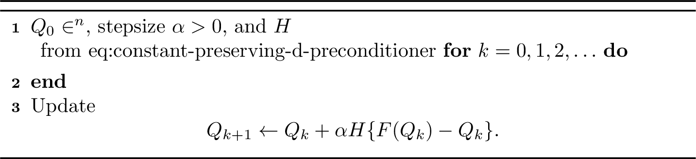
The proposed construction replaces the stochastic weighting matrix \(D\) in the update of 1 with the correction matrix \(H\). The resulting algorithm is given in 2 and is called corrected Q-learning (CQL). To analyze its fixed point, define the corresponding map \[g(Q):=Q+\alpha H\{F(Q)-Q\}. \label{eq:cpd-standard-map}\tag{1}\] The next lemma shows that the correction does not move the Bellman fixed point \(Q^\star\).

Subtracting \(Q^\star=F(Q^\star)\) from the update in 2 gives the error recursion \[\begin{align} Q_{k+1}-Q^\star=(Q_k-Q^\star) +\alpha H\{F(Q_k)-F(Q^\star)-(Q_k-Q^\star)\}.\label{eq:1} \end{align}\tag{2}\]

We next show that the error recursion in 2 admits an exact SLS representation.

The corresponding switching family associated with deterministic policies is \[\mathcal{A}^{\rm CQL} :=\left\{A_\pi^{\rm CQL}:\pi\in\Theta\right\}.\] It follows directly that, for every stochastic selector \(\mu_k\), \(A_{\mu_k}^{\rm CQL}\in\operatorname{co}(\mathcal{A}^{\rm CQL})\). Using the identity in ?? , one can prove that every switching mode in \(\operatorname{co}(\mathcal{A}^{\rm CQL})\) has a common eigenvector.

Therefore, the all-ones direction is again a common invariant direction, equivalently a common eigenvector, with scalar factor \(1-\alpha\delta(1-\gamma)\). Throughout the paper, we require this factor to lie strictly between zero and one so that each mode in \(\operatorname{co}(\mathcal{A}^{\rm CQL})\) is stable before any momentum is added.

The correction matrix \(H\) should be viewed as a structural correction rather than as a universal accelerator. It is introduced in place of \(D\) to recover the common eigenvector property in ?? for all switching modes. This property alone does not imply that CQL is always faster than QL. The value of \(H\) is that it creates the decomposition needed to certify the acceleration of the heavy-ball CQL recursion introduced next. Indeed, adding a heavy-ball momentum term directly to QL may also improve convergence, and in some instances it may even be faster than CQL with a heavy-ball momentum term. The difficulty is that, without the common eigenvector in ?? , an analogous JSR-based certificate is harder to obtain for the heavy-ball QL without the modification. The subsequent theory and numerical examples show cases in which CQL with momentum is both theoretically certified and empirically observed to be faster than the corresponding corrected or standard baseline.

The analysis in this paper separates this all-ones direction from its orthogonal complement. For this purpose, we introduce the following projection and the associated projected SLS. Let \(U\in\mathbb{R}^{n\times(n-1)}\) have orthonormal columns spanning \(\operatorname{span}\{\mathbf{1}\}^\perp\), so that \(U^\top U=I_{n-1}\), \(U^\top\mathbf{1}=0\), and \(UU^\top=I-n^{-1}\mathbf{1}\mathbf{1}^\top\). Define the projected standard family \[\bar A_\pi^{\rm CQL}:=U^\top A_\pi^{\rm CQL}U, \qquad \bar{\mathcal{A}}^{\rm CQL} :=\left\{\bar A_\pi^{\rm CQL}:\pi\in\Theta\right\}. \label{eq:cpd-projected-standard-family}\tag{3}\] The matrix \(\bar A_\pi^{\rm CQL}\) is the mode induced by \(A_\pi^{\rm CQL}\) on the orthogonal component. The next lemma makes this statement precise at each iteration.

This decomposition gives a direct expression for the full JSR \(\rho(\mathcal{A}^{\rm CQL})\) in terms of the constant scalar block corresponding to the common eigenvector and the projected SLS family \(\bar{\mathcal{A}}^{\rm CQL}\).

The decomposition immediately implies that the projected SLS family \(\bar{\mathcal{A}}^{\rm CQL}\) cannot have a larger JSR than the full SLS family \({\mathcal{A}}^{\rm CQL}\).

The same decomposition also gives the corresponding lower bound for the constant scalar mode.

This paper focuses on the case in which the projected SLS family \(\bar{\mathcal{A}}^{\rm CQL}\) is strictly faster than the full SLS family \({\mathcal{A}}^{\rm CQL}\). In that regime, the decomposition in ?? shows that the standard rate is governed by the common all-ones eigenvalue. The proposed modifications can then improve convergence along the corresponding invariant direction without being blocked by the projected SLS dynamics represented by \(\bar{\mathcal{A}}^{\rm CQL}\).

Under this assumption, the decomposition in ?? shows that \(\rho(\mathcal{A}^{\rm CQL})\) is exactly the eigenvalue of the common all-ones eigenvector.

Combining [ass:cpd-projected-gap,lem:cpd-standard-benchmark] with 1, we obtain the equivalent form \[\rho(\bar{\mathcal{A}}^{\rm CQL})<1-\alpha\delta(1-\gamma)<1.\]

The projected modes given in 3 have a useful structural feature: the tuning parameter \(\delta\) affects only the common all-ones direction, not the projected dynamics. This result is formally summarized in the following.

Intuitively, changing \(\delta\) moves only the all-ones common eigenvalue in ?? , while leaving the projected SLS family in 3 unchanged by ?? . This separation is useful when choosing \(\delta\): it allows dynamics along the common eigenvector direction to be tuned without changing the projected JSR term that appears in ?? .

5 Heavy-ball corrected Q-learning↩︎

Before introducing the corrected heavy-ball recursion, it is useful to contrast it with the deterministic heavy-ball Q-value iteration studied in [29]. That work considers the unweighted heavy-ball Q-value iteration update \[Q_{k+1} =Q_k+\alpha\{F(Q_k)-Q_k\}+\eta(Q_k-Q_{k-1}). \label{eq:unweighted-hb-qvi-update}\tag{4}\] Its acceleration mechanism is to improve the convergence rate along the common eigenvector direction. A stochastic heavy-ball Q-learning analogue, however, has the conditional mean dynamics \[Q_{k+1}=Q_k+\alpha D\{F(Q_k)-Q_k\}+\eta(Q_k-Q_{k-1}),\] in which the diagonal sampling matrix \(D\) multiplies the Bellman residual. As noted after 1, this multiplication generally destroys the common eigenvector property unless \(D\) is uniform. The corrected matrix \(H\) in ?? is introduced precisely to retain nonuniform sampling weights while restoring the common eigenvector direction needed by the JSR analysis below.

This section studies the effect of adding a heavy-ball momentum term to the CQL update in 2. The resulting update is given in 3 and is called heavy-ball corrected Q-learning (HBCQL).

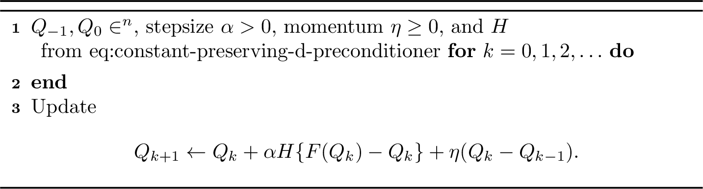
To proceed, define the augmented map \[g(Q,Q^-) := \begin{bmatrix} Q+\alpha H\{F(Q)-Q\}+\eta(Q-Q^-)\\ Q \end{bmatrix}.\] The augmented map has the same fixed point in both blocks as the corrected standard map in 1 .

Subtracting \(Q^\star=F(Q^\star)\) from the HBCQL update in 3 gives the error recursion \[\begin{align} Q_{k+1}-Q^\star &=(Q_k-Q^\star) +\alpha H\{F(Q_k)-F(Q^\star)-(Q_k-Q^\star)\} +\eta\{(Q_k-Q^\star)-(Q_{k-1}-Q^\star)\}.\label{eq:2} \end{align}\tag{5}\] The next lemma shows that the error recursion in 5 can be expressed as an SLS.

The corresponding SLS family is defined and denoted by \[\mathcal{A}^{\rm HBCQL} :=\left\{A_\pi^{\rm HBCQL}:\pi\in\Theta\right\}. \label{eq:cpd-hb-family}\tag{6}\] Moreover, for every stochastic selector \(\mu_k\), one has \(A_{\mu_k}^{\rm HBCQL}\in\operatorname{co}(\mathcal{A}^{\rm HBCQL})\). For the augmented heavy-ball recursion, the one-dimensional common eigenvector argument on \(\operatorname{span}\{\mathbf{1}\}\) becomes an argument with respect to a two-dimensional invariant subspace. To show this, define the subspace \[\mathcal{I} :=\left\{ \begin{bmatrix}a\mathbf{1}\\ b\mathbf{1}\end{bmatrix}:a,b\in\mathbb{R} \right\}. \label{eq:cpd-hb-constant-subspace}\tag{7}\] If the augmented error belongs to this subspace, then the next augmented error also belongs to it, and the scalar coefficients are updated by the following \(2\times2\) matrix: \[C:= \begin{bmatrix} \bigl(1-\alpha\delta(1-\gamma)\bigr)+\eta&-\eta\\ 1&0 \end{bmatrix}.\] This invariance is summarized in the next lemma.

Thus, the common eigenvector direction \(\operatorname{span}\{\mathbf{1}\}\) of CQL is lifted, in HBCQL, to the invariant subspace \(\mathcal{I}\) of the augmented state. On \(\operatorname{span}\{\mathbf{1}\}\), CQL follows the first-order scalar dynamics \[x_{k+1}=\bigl(1-\alpha\delta(1-\gamma)\bigr)x_k,\quad x_k\in \operatorname{span}\{\mathbf{1}\},\] whereas HBCQL follows the second-order dynamics on \(\mathcal{I}\) governed by the matrix \(C\) in ?? as follows: \[x_{k+1}=Cx_k,\quad x_i \in {\mathcal{I}}.\] The preceding lemma therefore implies that the augmented SLS family of HBCQL cannot have a JSR smaller than the spectral radius of \(C\). To explain this, define, for any stochastic policy \(\mu\), the following projected mode and its associated SLS family: \[\bar A_\mu^{\rm HBCQL}:= \begin{bmatrix} U^\top A_\mu^{\rm CQL}U+\eta I_{n-1}&-\eta I_{n-1}\\ I_{n-1}&0 \end{bmatrix}, \qquad \bar{\mathcal{A}}^{\rm HBCQL} :=\left\{\bar A_\pi^{\rm HBCQL}:\pi\in\Theta\right\}. \label{eq:cpd-projected-hb-family}\tag{8}\] The next lemma shows that the projected augmented error associated with ?? can be represented by an SLS.

As in the CQL analysis, we can now decompose the augmented SLS family in 6 into the constant-error subspace in 7 and the projected dynamics in 8 .

The decomposition in ?? gives the following two lower bounds.

A natural question is whether the HBCQL recursion can improve the convergence rate. The common eigenvector direction can be accelerated by a suitable positive momentum. The next theorem gives a sufficient condition under which HBCQL has a strictly smaller JSR than CQL.

1 implies that, under its hypotheses, HBCQL converges to \(Q^\star\) and has a strictly smaller JSR certificate than the CQL recursion in 2. Note that 1 assumes the strict inequality in 2. Because this condition may be hard to verify directly, the following corollary gives a simple sufficient interval for \(\delta\) that automatically guarantees 2.

6 Hyperparameter conditions for improving over standard Q-learning↩︎

The previous theorem compares HBCQL with CQL (\(\eta =0\)). We also state a useful sufficient condition under which HBCQL is faster than the standard QL benchmark in 1, obtained by setting the momentum term to zero and not applying the correction. Since \(D\) is nonsingular, the fixed point of 1 is \(Q^\star\). Subtracting \(Q^\star=F(Q^\star)\) from the update given in 1 gives the error recursion \[\begin{align} Q_{k+1}-Q^\star &=(Q_k-Q^\star) +\alpha D\{F(Q_k)-F(Q^\star)-(Q_k-Q^\star)\}.\label{eq:3} \end{align}\tag{9}\] The next lemma uses ?? to derive an SLS model associated with the error recursion in 9 .

The corresponding SLS family is \[\mathcal{A}^{\rm QL}:=\left\{A_\pi^{\rm QL}:\pi\in\Theta\right\}. \label{eq:direct-d-standard-family}\tag{10}\] We now compare CQL with the standard QL benchmark. The correction in CQL is designed to preserve a common eigenvector, but this structural property alone does not imply an improvement over QL. The next result gives a sufficient condition under which the JSR of CQL is no larger than that of the QL benchmark.

The remaining question is whether HBCQL can be faster than the QL benchmark itself. Combining the previous comparison with the heavy-ball improvement theorem 1 gives the following sufficient condition for a strict JSR comparison of HBCQL against QL.

The previous lemma packages two requirements into the interval for \(\delta\): the upper bound gives the hypotheses of 1, while \(d_{\max}\le\delta\) gives the comparison between CQL and QL. The following corollary separates these two roles. It assumes the projected gap directly and states the conclusion in terms of the hyperparameters.

7 Numerical illustration↩︎

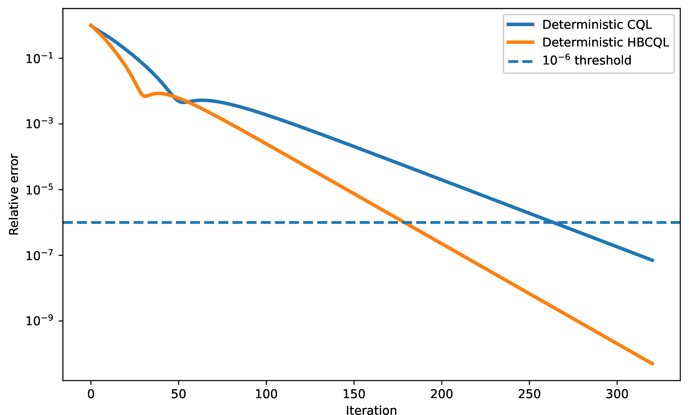
This section gives an example for [alg:cpd-standard-update,alg:cpd-hb-update]. The purpose of this example is to show in a reproducible finite example how the heavy-ball momentum term can accelerate convergence. We consider an MDP with \(\mathcal{S}=\{1,2\}\), \(\mathcal{A}=\{1,2\}\), and \(\gamma=0.9\). The transition-to-next-state probabilities are \[P_s= \begin{bmatrix} 0.85&0.15\\ 0.70&0.30\\ 0.25&0.75\\ 0.10&0.90 \end{bmatrix}.\] The one-step reward entries are \(r(1,1,1)=r(1,1,2)=1.0\), \(r(1,2,1)=r(1,2,2)=0.2\), \(r(2,1,1)=r(2,1,2)=0.1\), and \(r(2,2,1)=r(2,2,2)=0.8\). The nonuniform sampling vector is set to \(d=(0.45,0.05,0.40,0.10)^\top\) and \(D=\operatorname{diag}(d)\), and the shared numerical parameters are \[\alpha=1.10, \qquad \delta=0.80, \qquad \eta=0.30.\] For the simulation, we use the initial values \(Q_{-1}=Q_0=(3,-2.5,1.5,0)^\top\), and the optimal Q-function is obtained by value iteration and is \(Q^\star\approx (9.16923,8.28615,7.93692,8.55385)^\top\). For comparative analysis, define the relative error \[e_k^Q=\frac{\left\|Q_k-Q^\star\right\|_2}{\left\|Q_0-Q^\star\right\|_2}.\] 4 compares 2 and 3. The figure shows that HBCQL reduces the relative error faster than CQL on this instance.

8 Stochastic heavy-ball corrected Q-learning↩︎

This section studies a model-free stochastic counterpart of the HBCQL recursion in 3. We first recall standard tabular Q-learning. Given \(Q_k\), draw \(i_k=(s_k,a_k)\sim d\), draw \(s_k^\prime\sim P(\cdot\mid s_k,a_k)\), and define \(\Delta_k:=r(s_k,a_k,s_k^\prime)+\gamma\max_{b\in\mathcal{A}}Q_k(s_k^\prime,b)-Q_k(s_k,a_k)\). The standard sampled update changes the sampled coordinate only: \[Q_{k+1}=Q_k+\alpha_k\Delta_ke_{i_k}.\] Equivalently, it can be written as \[Q_{k+1}(s,a)= \begin{cases} Q_k(s,a)+\alpha_k\Delta_k, & (s,a)=i_k,\\ Q_k(s,a), & (s,a)\ne i_k . \end{cases}\] The complete procedure is stated in 5.

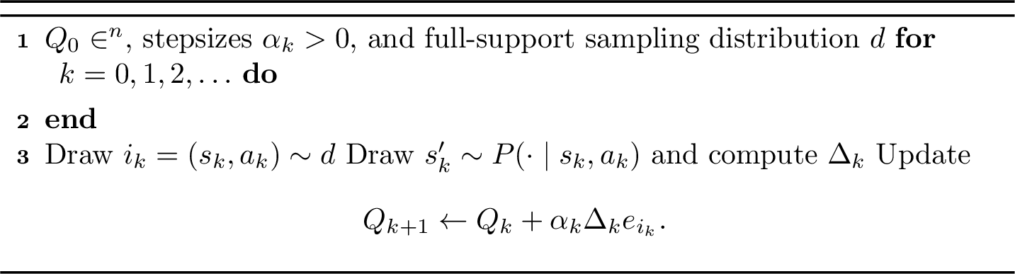
Throughout this section, samples are drawn i.i.d. from the full-support distribution \(d\). Markovian sampling is not treated here in order to keep the presentation focused, but the same conditional-mean switching viewpoint can be combined with Markovian stochastic-approximation tools, as in [15]. A replay buffer can also be used to approximate the independent sampling required below, following the experience-replay idea used in deep Q-networks (DQN) [3].

We now consider a sampled counterpart of the HBCQL in 3. At time \(k\), we sample \[i_k\sim d, \qquad j_k\sim d,\] where \(j_k\) is independent of \(i_k\) and of the transition sample used below. After \(i_k=(s_k,a_k)\) is selected, draw \(s'_k\) according to \(P(\cdot\mid s_k,a_k)\) and form \[\Delta_k :=r(s_k,a_k,s'_k) +\gamma\max_{b\in\mathcal{A}}Q_k(s'_k,b)-Q_k(s_k,a_k). \label{eq:sampled-hb-td-error}\tag{11}\] The stochastic HBCQL is written as \[Q_{k+1} =Q_k +\alpha\Delta_k\bigl(e_{i_k}+\delta\mathbf{1}-e_{j_k}\bigr) +\eta(Q_k-Q_{k-1}). \label{eq:sampled-hb-d-randomized-update}\tag{12}\] For each state-action pair \((s,a)\), this is equivalently written as \[Q_{k+1}(s,a) =Q_k(s,a) +\alpha\Delta_k \left(\mathbf{1}_{\{(s,a)=i_k\}}+\delta-\mathbf{1}_{\{(s,a)=j_k\}}\right) +\eta\{Q_k(s,a)-Q_{k-1}(s,a)\}.\] The complete pseudocode is given in 6.

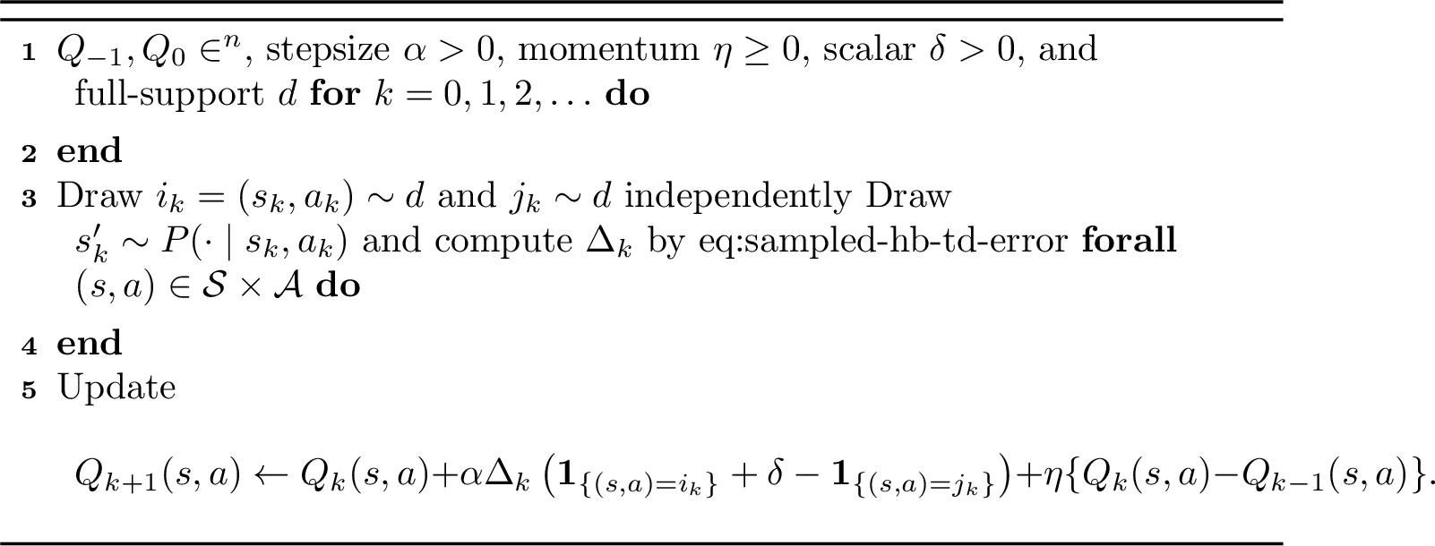
Setting \(\eta=0\) in 6 gives the sampled stochastic version of CQL. Compared with classical Q-learning, the update uses two independent state-action indices, \(i_k\) and \(j_k\). This increases the sampling burden, but it is not the double-sampling issue associated with residual-gradient methods in [30]: only one next-state sample is drawn from the selected pair \(i_k\), while the second draw is an independent state-action index used to approximate the centering term. In practice, the second index can be drawn from a replay buffer. Equivalently, with the noise \[\xi_{k+1} :=\Delta_k\bigl(e_{i_k}+\delta\mathbf{1}-e_{j_k}\bigr) -H\{F(Q_k)-Q_k\},\] one has \(\mathbb{E}[\xi_{k+1}\mid Q_k,Q_{k-1}]=0\), and the recursion in 12 can equivalently be written as \[Q_{k+1} =Q_k+ \alpha H\{F(Q_k)-Q_k\} +\eta(Q_k-Q_{k-1}) +\alpha\xi_{k+1}. \label{eq:sampled-hb-d-randomized-noise-form}\tag{13}\] The noise form in 13 shows that 12 is an unbiased stochastic approximation of the deterministic HBCQL update in 3. The next lemma gives the corresponding conditional-mean identity.

The conditional-mean update in ?? is exactly the deterministic HBCQL recursion analyzed in the previous section. Hence its right-hand side admits the same SLS representation as ?? . Therefore, the deterministic HBCQL JSR certificates apply to the conditional-mean recursion associated with 12 . When the corresponding JSR is smaller than one, finite-time error bounds can be derived by applying the Lyapunov-based SLS analysis in [15]. The convergence and acceleration conclusions established for deterministic HBCQL therefore transfer to this conditional-mean recursion, so we omit the repeated argument.

9 Numerical illustration↩︎

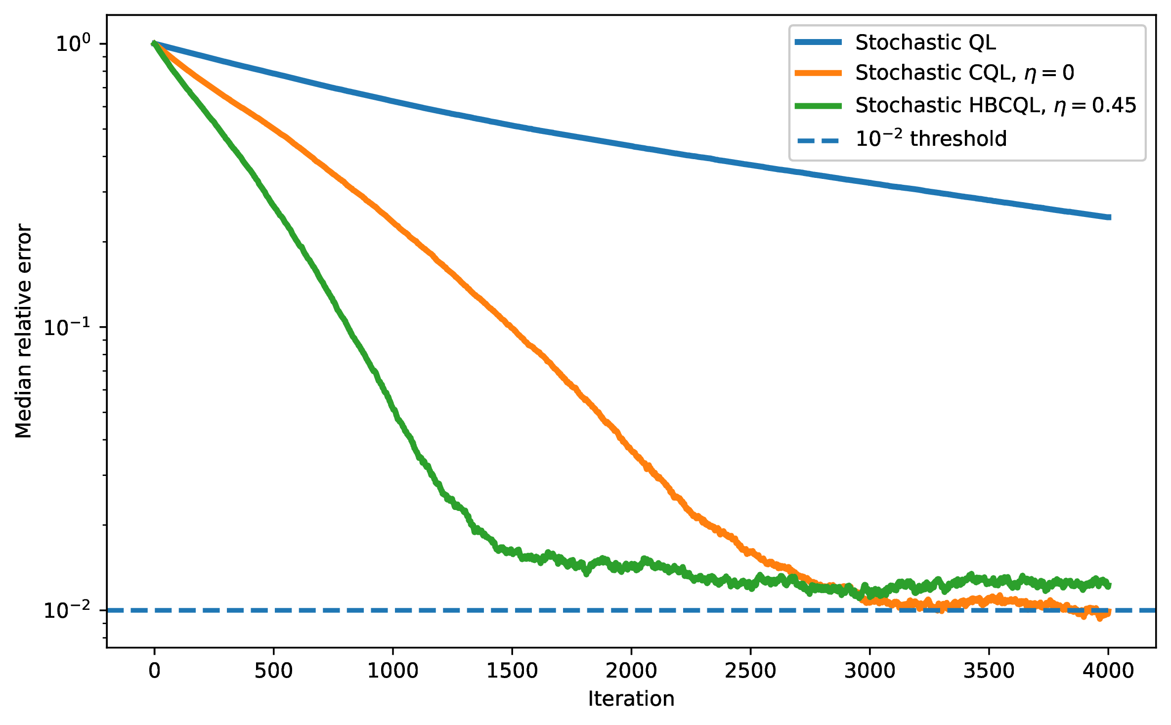
This section adds an experiment for 6, where we use the same MDP and parameter settings as in 7. The only change is that the Bellman residual is now observed through transition samples rather than evaluated as a full vector. We compare two choices of this update, \(\eta=0\) (CQL counterpart) and \(\eta=0.45\) (HBCQL), against standard tabular Q-learning with the same samples. All three methods are run with common random numbers, so differences between the curves are not due to different random seeds. The numerical parameters are \(\alpha=0.020\), \(\delta=0.80\), \(\eta\in\{0,0.45\}\), and \(K=4000\). The reported curve is the median over \(400\) independent Monte Carlo paths of the relative error \[e_k^{\rm mc} =\frac{\|Q_k-Q^\star\|_2}{\|Q_0-Q^\star\|_2}.\] Because the stepsize is constant, the stochastic methods should be interpreted as approaching a noise neighborhood of \(Q^\star\), not as converging exactly to zero error. 7 shows the median relative \(Q\)-error curves. The CQL update (\(\eta=0\)) is already much faster than standard Q-learning in this nonuniformly sampled example. Adding the heavy-ball term gives a further transient acceleration: the median first passage time below \(10^{-2}\) drops from about \(2693\) iterations to about \(1556\) iterations.

10 Corrected Q-learning with linear function approximation↩︎

The correction method from the previous sections can be extended to deterministic Q-learning with linear function approximation, referred to as linear Q-learning (LQL). Let the parameter vector be \(\theta\in\mathbb{R}^m\), and approximate the Q-vector by \(\Phi\theta\in\mathbb{R}^n\), where the feature matrix \(\Phi\in\mathbb{R}^{n\times m}\) has one row for each state-action pair and one column for each feature. We impose the standard rank condition on the feature matrix.

To use the ideas from the previous sections, we introduce the following assumption.

This assumption is easy to enforce in tabular feature constructions: one may include an intercept feature, namely a column of \(\Phi\) filled with ones. Then the corresponding coordinate vector can be chosen as \(c\). The standard deterministic LQL update is summarized in 8.

The corresponding map is defined as \[g(\theta):=\theta+\alpha\Phi^\top D\{F(\Phi\theta)-\Phi\theta\}.\] Its fixed points, \(g(\theta)=\theta\), are characterized by the associated residual equation below.

Subtracting the fixed-point identity in ?? from the update in 8 gives \[\begin{align} \theta_{k+1}-\bar\theta =\theta_k-\bar\theta +\alpha\Phi^\top D\{F(\Phi\theta_k)-F(\Phi\bar\theta) -\Phi(\theta_k-\bar\theta)\}.\label{eq:5} \end{align}\tag{14}\] The next lemma states an SLS error system associated with the above error recursion.

For the matrix in ?? , the modes generally do not share a common eigenvector. Consequently, the common-eigenvector acceleration argument used in the tabular analysis does not apply directly. To remove this obstruction, we introduce the corrected map below.

The map \(G\) has a structure similar to the tabular correction, as summarized in the following result.

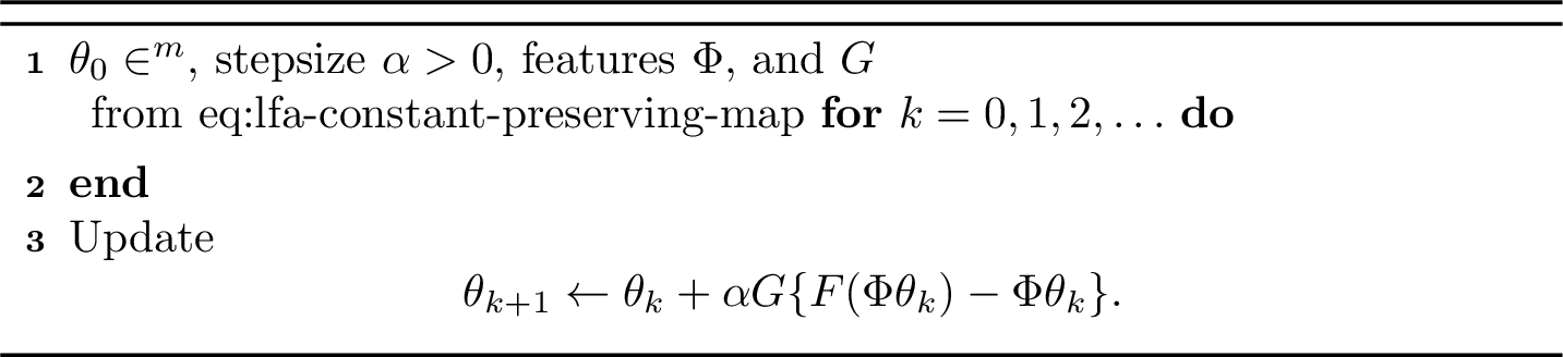
The corresponding deterministic corrected linear Q-learning (CLQL) is given in 9. Note that this is exactly the tabular correction when \(\Phi=I\) and \(c=\mathbf{1}\).

Define the corresponding feature-space map \[g(\theta) :=\theta+\alpha G\{F(\Phi\theta)-\Phi\theta\}. \label{eq:lfa-cpd-standard-map}\tag{15}\] The next lemma characterizes the fixed points of this map.

Unlike the tabular matrix \(H\), the map \(G\) is generally not nonsingular. It is often rectangular, since it maps a Bellman residual in \(\mathbb{R}^n\) to a parameter update in \(\mathbb{R}^m\), and even in the square case its rank depends on \(\Phi\), \(D\), \(d\), and \(c\). Hence, the feature-space analysis in the sequel uses the fixed-point equation in ?? and explicitly assumes uniqueness.

The fixed point condition in ?? should be compared with the standard LQL update in 8. A fixed point corresponding to the standard LQL satisfies \(\Phi^\top D\{F(\Phi\theta)-\Phi\theta\}=0\), which is the usual \(D\)-weighted projected Bellman equation: the Bellman residual is orthogonal to every feature column in the \(D\)-weighted inner product. By contrast, a fixed point of the update in 9 satisfies \(G\{F(\Phi\theta)-\Phi\theta\}=0\). Thus the two fixed-point equations generally need not have the same solution.

Next, subtracting the fixed-point equation in ?? from the update in 9 gives the error recursion \[\begin{align} \theta_{k+1}-\theta^\star =(\theta_k-\theta^\star)+ \alpha G\{F(\Phi\theta_k)-F(\Phi\theta^\star) -\Phi(\theta_k-\theta^\star)\}.\label{eq:4} \end{align}\tag{16}\] We next rewrite this error recursion as an SLS.

The corresponding SLS family is \[\mathcal{A}^{\rm CLQL} :=\left\{A_\pi^{\rm CLQL}:\pi\in\Theta\right\}.\] As in the tabular case, every mode in \(\mathcal{A}^{\rm CLQL}\) has a common eigenvector as shown below.

By ?? , the direction \(\operatorname{span}\{c\}\) is a common eigenvector direction of the SLS family \(\mathcal{A}^{\rm CLQL}\). As in the tabular analysis, we decompose the feature-space dynamics into this common direction and the induced dynamics on the quotient space. This decomposition provides the same type of convergence benchmark as in the tabular analysis. Let \(\bar{\mathcal{A}}^{\rm CLQL}\) denote the quotient family induced by \(\mathcal{A}^{\rm CLQL}\) on \(\mathbb{R}^m/\operatorname{span}\{c\}\).

The decomposition in ?? immediately gives the following lower bounds.

As in the tabular case, acceleration is certified under a strict JSR gap between the full SLS family \(\mathcal{A}^{\rm CLQL}\) and the projected SLS family \(\bar{\mathcal{A}}^{\rm CLQL}\) as summarized in the following assumption.

Under 6, the decomposition in ?? shows that \(\rho(\mathcal{A}^{\rm CLQL})\) is identical to the eigenvalue associated with the common eigenvector direction.

We now add the heavy-ball momentum term to the CLQL recursion in 9. The resulting algorithm is summarized in 10 and is called heavy-ball corrected linear Q-learning (HBCLQL).

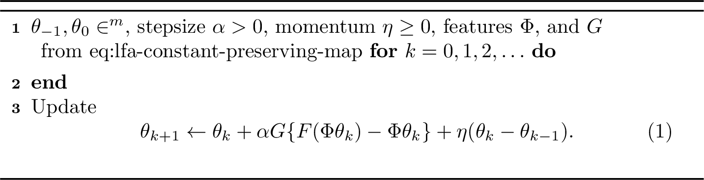
The next lemma writes the resulting second-order error recursion as a first-order augmented SLS.

The corresponding SLS family is given by \[\mathcal{A}^{\rm HBCLQL} :=\left\{A_\pi^{\rm HBCLQL}:\pi\in\Theta\right\}. \label{eq:lfa-cpd-hb-family}\tag{17}\] As in the tabular case, the augmented feature-space dynamics preserve the subspace \[{\mathcal{I}}:=\left\{ \begin{bmatrix}ac\\bc\end{bmatrix}:a,b\in\mathbb{R} \right\} \subset \mathbb{R}^{2m}.\] Indeed, for every policy \(\mu\), [eq:lfa-cpd-common-vector,eq:lfa-cpd-hb-mode] imply that \(A_\mu^{\rm HBCLQL}\) maps any vector in \({\mathcal{I}}\) to another vector in \({\mathcal{I}}\). If the augmented error belongs to this subspace, then the next augmented error also belongs to it, and the scalar coefficients are updated by the following constant matrix: \[C := \begin{bmatrix} \bigl(1-\alpha\delta(1-\gamma)\bigr)+\eta&-\eta\\ 1&0 \end{bmatrix}.\]

Using the quotient basis from 1, define \[\bar A_\pi^{\rm HBCLQL} :=\begin{bmatrix}\bar A_\pi^{\rm CLQL}+\eta I_{m-1}&-\eta I_{m-1}\\ I_{m-1}&0\end{bmatrix}, \qquad \bar{\mathcal{A}}^{\rm HBCLQL} :=\left\{\bar A_\pi^{\rm HBCLQL}:\pi\in\Theta\right\}.\] The block-triangular decomposition in the same basis gives \[\rho(\mathcal{A}^{\rm HBCLQL}) =\max\{\rho(C),\rho(\bar{\mathcal{A}}^{\rm HBCLQL})\}. \label{eq:lfa-cpd-hb-jsr-decomposition}\tag{18}\] The next theorem gives conditions under which HBCLQL converges faster than CLQL.

This result establishes a condition in which HBCLQL improves over CLQL. Conditions under which both HBCLQL and CLQL improve over LQL can be obtained by the same argument as in the tabular case; the details are omitted to avoid repetition.

11 Numerical illustration↩︎

This example compares [alg:lfa-direct-phi-d-update,alg:lfa-cpd-standard-update,alg:lfa-cpd-hb-update]. We use the same two-state, two-action MDP as in 7, together with the feature matrix specified below. Throughout this comparison, we use the parameters \(\alpha=2.5,\delta= 2,\eta = 0.1\), and \[\Phi= \begin{bmatrix} 1& 1& 1\\ 1& 1&-1\\ 1&-1& 1\\ 1&-1&-1 \end{bmatrix},\] and one verifies that \(c=(1,0,0)^\top\) satisfies \(\Phi c=\mathbf{1}\). The feature recursions use \(\theta_{-1}=\theta_0=(3,-2.5,1.5)^\top\). In this example, the fixed points of LQL and CLQL coincide numerically: \[\theta^\star\approx(6.21874,0.75652,0.02213)^\top, \qquad \Phi\theta^\star\approx(6.99739,6.95313,5.48435,5.44009)^\top .\] For the comparison, we define the relative error \[e_k^\theta=\frac{\left\|\theta_k-\theta^\star\right\|_2}{\left\|\theta_0-\theta^\star\right\|_2}.\] 11 compares the three algorithms. CLQL reaches the \(10^{-6}\) threshold after 22 iterations, compared with 28 iterations for LQL. Adding the small heavy-ball momentum term further reduces the hit time to 15 iterations. All three final relative parameter errors are at the \(10^{-15}\) scale by the end of the run.

The momentum parameter remains deliberately small in this illustration. Larger values of \(\delta\) or \(\eta\) can make the numerical comparison even more aggressive, but this moderate setting already shows the intended ordering: CLQL is faster than the direct feature recursion, and HBCLQL is faster than CLQL on this instance.

12 Sampled stochastic heavy-ball linear function approximation↩︎

Based on the deterministic HBCLQL analysis, this section extends the sampled model-free construction to linear function approximation. For comparison, we first recall sampled Q-learning with linear function approximation. Let \(Q_k=\Phi\theta_k\). Given \(\theta_k\), draw \(i_k=(s_k,a_k)\sim d\), draw \(s_k^\prime\sim P(\cdot\mid s_k,a_k)\), and define \[\Delta_k :=r(s_k,a_k,s_k^\prime) +\gamma\max_{b\in\mathcal{A}}(\Phi\theta_k)(s_k^\prime,b) -(\Phi\theta_k)(s_k,a_k). \label{eq:sampled-standard-lfa-q-learning-td-error}\tag{19}\] The corresponding standard linear Q-learning update is given in 12.

We now consider a stochastic HBCLQL counterpart. Set \(Q_k=\Phi\theta_k\) and start from \(\theta_{-1},\theta_0\in\mathbb{R}^m\). At time \(k\), we draw \(i_k\sim d\) and \(j_k\sim d\) independently. If \(i_k=(s_k,a_k)\), draw \(s'_k\sim P(\cdot\mid s_k,a_k)\) and form \[\Delta_k :=r(s_k,a_k,s'_k) +\gamma\max_{b\in\mathcal{A}}(\Phi\theta_k)(s'_k,b) -(\Phi\theta_k)(s_k,a_k). \label{eq:sampled-lfa-hb-td-error}\tag{20}\] The parameter is then updated as in 13.

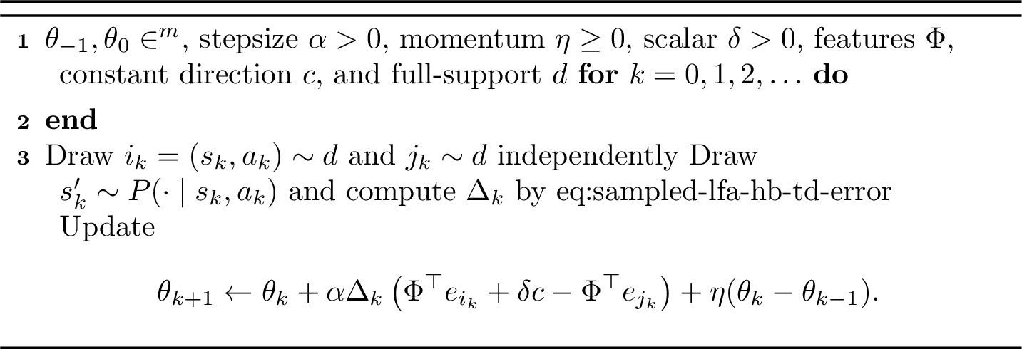
The update in 13 is an unbiased stochastic approximation of the deterministic HBCLQL recursion in [eq:lfa-cpd-hb-update]. The next lemma summarizes this conditional-mean relation.

By the same argument used in 30, the right-hand side of ?? is represented by the SLS in ?? . Therefore, the convergence and acceleration certificates for stochastic HBCLQL hold at the conditional-mean level by the deterministic analysis in 10. A full stochastic RL analysis, including martingale noise, constant-stepsize neighborhoods, and Markovian sampling, can be developed by combining this drift representation with Lyapunov-based stochastic approximation arguments as in [15]. We do not repeat those technical steps here.

13 Numerical illustration↩︎

Consider again the example in 11, where the MDP, feature matrix, sampling distribution \(d\), constant direction \(c\), initial parameter, and fixed point \(\theta^\star\) are the same as in that section. We use the constant stepsize \(\alpha=0.002\), the correction parameter \(\delta=2\), and the momentum parameter \(\eta=0.1\) for HBCLQL. Stochastic CLQL is obtained from 13 by setting \(\eta=0\), while stochastic LQL uses 12. The three methods are run for \(12{,}000\) iterations over \(400\) independent sample paths. To make the comparison depend on the update rule rather than sampling variation, the same sampled state-action pairs, centering samples, and next-state draws are used across the methods whenever applicable.

The quantity in 14 is the median, over the \(400\) paths, of the relative parameter error \(e_k^\theta\) defined in 11. In this run, stochastic HBCLQL reaches median error \(10^{-1}\), \(5\times10^{-2}\), and \(2\times10^{-2}\) after \(4074\), \(5418\), and \(7177\) iterations, respectively. Stochastic CLQL reaches the same thresholds after \(4560\), \(6036\), and \(8202\) iterations, while stochastic LQL reaches the first two thresholds after \(6840\) and \(9219\) iterations and does not reach \(2\times10^{-2}\) within \(12{,}000\) iterations. Thus the sampled experiment preserves the early-stage ordering observed in the deterministic example in 11. At later iterations, stochastic fluctuations produce a small neighborhood around the fixed point, so the final curves need not remain strictly ordered.

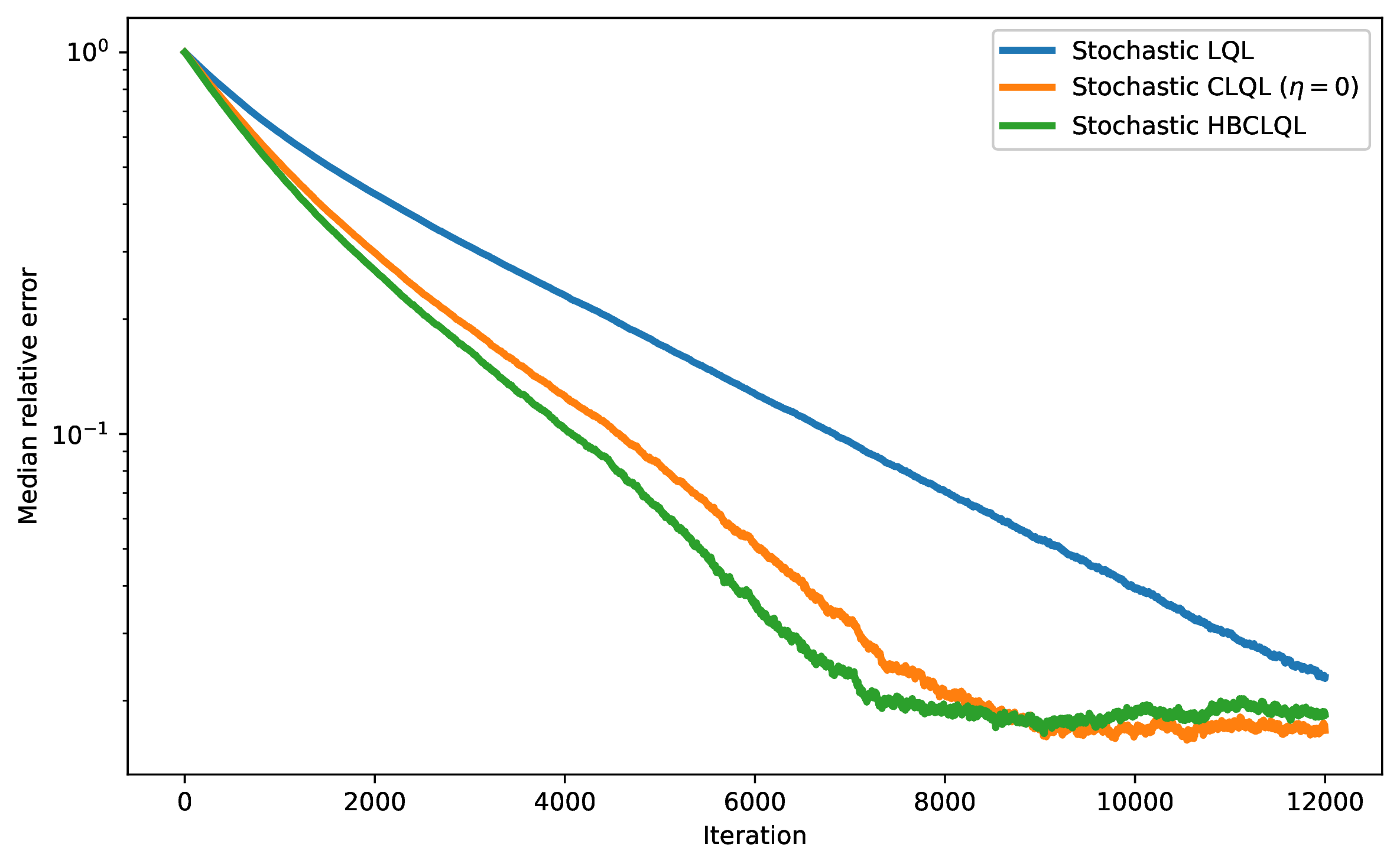
14 Conclusion↩︎

This paper proposed CQL and combined it with heavy-ball momentum. The analysis used SLS and JSR tools to separate the dynamics along a common eigenvector direction from the dynamics along the orthogonal directions. Under the stated projected-gap and small-momentum conditions, HBCQL has a smaller JSR certificate than CQL, and analogous statements hold for linear function approximation.

15 Auxiliary results↩︎

15.1 Nonnegative matrix row-sum bounds↩︎

The following standard row-sum bound is the form of the Collatz–Wielandt inequality used below; see, for example, [31].

15.2 Standard JSR lemmas↩︎

This standard property follows from norm equivalence in the definition of the JSR; see, for example, [14].

15.3 Feature-space two-point difference identity↩︎

The following identity is the two-point version of the fixed-point error system in 26. It is placed in the appendix because the main feature-space development only needs the fixed-point form.

15.4 Jury stability criterion↩︎

The proof is omitted; see [32].

15.5 Scalar heavy-ball acceleration conditions↩︎

References↩︎