Pretrained Time-Series Foundation Models for Financial Return Forecasting
June 25, 2026
Abstract
Financial return forecasting is a difficult test case for time-series foundation models because daily equity returns combine low signal-to-noise ratios, structural breaks, heavy tails, and weak persistence. This paper benchmarks pretrained time-series foundation models (TSFMs) against train-from-scratch neural baselines in a deliberately conservative financial setting. We evaluate TimeGPT/TimeGPT-LH, TimesFM-2.5, Moirai-2.0, Chronos, and Chronos-2 against NBEATS, NHITS, PatchTST, iTransformer, and KAN on five liquid U.S. equities (AAPL, AMZN, GOOG, JPM, and META), using both linear and log returns. All neural models are compared under an equalized context budget of \(L=512\) observations, a rolling-origin protocol, and error metrics benchmarked against naive random-walk alternatives. The paper also provides a compact theoretical framing of pretraining as an inductive prior, linking PAC-Bayes transfer intuition, information-theoretic predictability limits, attention geometry, and score-distribution comparisons to the empirical design. This framing clarifies why strong rankings need not imply economically meaningful predictability in noisy markets. The main finding is pragmatic rather than sensational. Pretrained TSFMs dominate the ranking distribution, accounting for 8 of 10 task-level wins, with Moirai-2.0 and TimesFM-2.5 achieving the strongest average ranks. TimesFM-2.5 leads the AAPL and JPM tasks, Moirai-2.0 leads the GOOG tasks and one AMZN task, and Chronos wins the remaining AMZN task. However, the iTransformer baseline wins both META tasks, showing that local supervised learning can still outperform generic pretraining for specific assets and regimes. More importantly, gains over the random-walk benchmark are small and sparse. A one-sided Diebold–Mariano test rejects equal or inferior predictive accuracy only for Chronos on AMZN and Moirai-2.0 on GOOG. The evidence therefore supports TSFMs as useful practical priors that reduce model-development costs in low-data financial forecasting, but not as universal engines of statistically reliable alpha generation or trading performance in realistic empirical deployment conditions.
Pretrained Time-Series Foundation Models for Financial Return Forecasting
Miquel Noguer i Alonso\(^{1}\)Rodolfo Pereira Franklin\(^{1}\)
\(^{1}\)Artificial Intelligence Finance Institute
2026-06-26
Keywords: Time-series foundation models; financial return forecasting; pretrained forecasting models; equity returns; rolling-origin evaluation; Diebold–Mariano test; TimeGPT; TimesFM; Chronos; Moirai; neural forecasting.
1 Introduction↩︎
Time series analysis has long been a fundamental pillar of stochastic modelling, with its formal foundations in autoregressive models dating back to Yule and Walker in the 1920s and 1930s, and taking its modern form with the systematic ARMA framework of [1]. Forecasting financial returns within this tradition is notoriously difficult: signal-to-noise ratios are low, structural breaks are common, and even modest errors can erase any practical edge once trading frictions are considered. Recent progress in pretrained sequence models has nevertheless renewed interest in whether large-scale temporal pretraining can provide a better inductive bias than training a separate model for each asset.
This literature now contains two related but distinct strands. One strand adapts text large language models (LLMs) to time series through reprogramming or prompting, as in Time-LLM [2], LLM4TS [3], and PromptCast [4]. As emphasized by [5], LLMs such as GPT-4 [6] and Gemini [7] exhibit remarkable transfer-learning capabilities in few-shot and zero-shot settings, motivating the broader hypothesis that pretrained sequence intelligence may transfer to temporal data. Building on our previous findings regarding the efficacy of general-purpose Large Language Models adapted for financial time series through reprogramming techniques [8], this benchmark aims to extend that inquiry into the emerging class of models natively designed for temporal data. A second strand develops dedicated time-series foundation models (TSFMs), including TimeGPT [9], TimesFM [10], Chronos [11], Chronos-2 [12], and Moirai-2.0 [13]. The present benchmark belongs much more clearly to the second strand: most evaluated systems are pretrained time-series models rather than reprogrammed text LLMs. For that reason, this paper uses the term pretrained TSFM throughout.
The question studied here is practical. If a practitioner has only one return series per asset, wants a 20-business-day forecast, and does not want to run heavy per-ticker model development, is an out-of-the-box TSFM preferable to a train-from-scratch alternative? To answer that question, we compare six pretrained TSFMs against five strong baselines: NBEATS [14], NHITS [15], PatchTST [16], iTransformer [17], and KAN [18].
The contribution of the paper is threefold. First, it provides a compact benchmark over two return representations, five liquid equities, and a rolling-origin protocol, with detailed architectural exposition of each evaluated model. Second, it reframes the evidence around pretrained time-series models rather than generic “LLM” claims. Third, it separates statistical distinguishability from directional superiority when interpreting Diebold–Mariano (DM) results, preventing sign confusion relative to the random-walk benchmark.
2 Related Work↩︎
A related but distinct line of work adapts frozen text LLMs to time-series data through prompting or reprogramming, as in Time-LLM [2], LLM4TS [3], and PromptCast [4]. This literature motivates the broader hypothesis that sequence pretraining can transfer across modalities, but it is not the empirical focus of this paper: we do not run a direct Time-LLM or LLM-reprogramming experiment.
The pretrained-TSFM literature is closer to the systems evaluated here. TimeGPT [9] emphasizes transfer learning for zero-shot forecasting. TimesFM is a decoder-only foundation model for time-series forecasting [10]. Chronos casts forecasting as a language modeling problem over quantized values [11], while Chronos-2 extends that philosophy to a broader universal-forecasting setting with multivariate and covariate support [12]. Moirai-2.0 is a decoder-only foundation model built around quantile forecasting and efficiency improvements [13].
A complementary line of contemporaneous work asks the related but distinct question of how far generic TSFM pretraining transfers to finance-specific data. [19] evaluate zero-shot inference, fine-tuning, and pre-training from scratch for several TSFM families on a broad global panel of excess-return observations. Their main finding is that off-the-shelf TSFMs underperform standard ensemble and neural benchmarks in zero-shot and fine-tuning regimes, while finance-native pretraining closes much of the gap and can produce stronger portfolio performance. Our benchmark differs in scope—single-asset 20-business-day forecasts on five U.S. equities, rather than next-day cross-sectional excess returns at the global level—but the two studies are mutually informative. Theirs argues that domain-specific pretraining matters when the goal is cross-sectional return prediction and portfolio formation; ours measures how the same off-the-shelf TSFMs fare against train-from-scratch deep baselines for per-asset forecast error. The qualitative messages are consistent: gains from generic TSFMs can be useful in a low-data per-asset setting, but they remain limited and should not be confused with finance-specific economic outperformance.
Against these pretrained models, the paper uses strong supervised baselines. NBEATS and NHITS remain influential MLP-style decomposition models [14], [15]. PatchTST and iTransformer are modern transformer baselines that model temporal dependencies in different ways [16], [17]. KAN brings spline-based Kolmogorov–Arnold parameterization to time-series prediction [18] and proves particularly relevant here because it is the only train-from-scratch model that consistently breaks into the top tier.
3 Methodology↩︎
This section collects the architectural background of the evaluated systems. It begins with a shared problem formulation, then describes each model individually. The exposition follows the canonical references for each architecture and is provided to make the benchmark self-contained.
3.1 Problem Formulation↩︎
Fix a probability space \((\Omega, \mathcal{F}, \mathbb{P})\) supporting a real-valued return process \((r_t)_{t \in \mathbb{Z}}\) adapted to its natural filtration \(\mathcal{F}_t = \sigma(r_s : s \le t)\). For an asset return at horizon \(h \ge 1\) we seek a measurable forecast \[\hat{r}_{t+h} = f_t\!\big(r_{t-L+1}, \ldots, r_t\big),\] based on a context window of length \(L\), where \(f_t\) ranges over a class \(\mathcal{F}\) of admissible predictors. In our experiments \(h\) runs over \(1, \ldots, H\) with \(H = 20\). For a strictly proper loss \(\ell : \mathbb{R} \times \mathbb{R} \to \mathbb{R}_{\ge 0}\) the population risk and the Bayes-optimal predictor are \[\mathcal{R}(f) = \mathbb{E}\!\left[\ell\!\big(f_t(\mathcal{F}_t),\, r_{t+h}\big)\right], \qquad f^\star_{t,h} \in \arg\min_{g \in L^0(\mathcal{F}_t)} \mathbb{E}\!\left[\ell(g, r_{t+h}) \mid \mathcal{F}_t\right].\] The two losses that organize the analysis below are squared loss and absolute loss, with qualitatively different optima.
3.1.0.1 Semimartingale framework.
It is convenient to view \((r_t)\) as the sequence of increments of a discrete-time process \(R_t = \sum_{s \le t} r_s\) adapted to \((\mathcal{F}_t)\). By the Doob decomposition, \(R_t = M_t + A_t\) splits uniquely into an \((\mathcal{F}_t)\)-martingale \(M_t\) with \(M_0 = 0\) and an \((\mathcal{F}_{t-1})\)-predictable process \(A_t\) of locally bounded variation [20]. The martingale-difference hypothesis \(\mathbb{E}[r_{t+h} \mid \mathcal{F}_t] = 0\) corresponds to \(A \equiv 0\), in which case \(r_t = \Delta M_t\) is the increment of a pure martingale. Under this null the random-walk benchmark introduced below is exactly the Bayes-optimal \(L^2\) predictor; departures from the null—predictable drifts, regime-switching means, calendar effects—are precisely what any non-trivial forecaster aims to exploit. Throughout this paper we work without imposing the martingale-difference null on \((r_t)\): the random walk is treated as a benchmark to beat, not as a maintained hypothesis.
3.1.0.2 Squared loss.
For \(\ell(\hat{r}, r) = (\hat{r} - r)^2\), the Bayes-optimal predictor is the conditional mean \(f^\star_{t,h}(\mathcal{F}_t) = \mathbb{E}[r_{t+h} \mid \mathcal{F}_t]\), and the minimum risk equals the expected conditional variance \(\mathbb{E}\,\mathrm{Var}(r_{t+h}\mid\mathcal{F}_t)\). Most foundation-model training objectives target this loss, either directly (TimesFM, Moirai’s quantile head specializes to a mean-like predictor at \(q=0.5\)) or via a quantized likelihood that converges to it under refinement (Chronos, Chronos-2).
3.1.0.3 Absolute loss.
For \(\ell(\hat{r}, r) = |\hat{r} - r|\), the Bayes-optimal predictor is the conditional median \(f^\star_{t,h}(\mathcal{F}_t) = \mathrm{med}(r_{t+h} \mid \mathcal{F}_t)\), and the minimum risk equals \(\mathbb{E}\big[\,|r_{t+h} - \mathrm{med}(r_{t+h}\mid\mathcal{F}_t)|\,\big]\). This is the reference for our reported MAE: any model whose conditional forecasts deviate systematically from the conditional median pays a penalty in MAE that no amount of mean-targeting can recover. Because most evaluated systems are trained to minimize a squared- or quantized-likelihood loss rather than absolute loss, the metric and the training objective are deliberately not aligned, and the benchmark therefore tests robustness to that misalignment alongside raw predictive skill.
3.1.0.4 The random-walk benchmark and two coinciding hypotheses.
The zero-return random-walk forecast \(\hat{r}^{\mathrm{RW}}_{t+h} \equiv 0\) corresponds, on daily liquid-equity data, to two distinct hypotheses that happen to coincide. First, under the martingale hypothesis \(\mathbb{E}[r_{t+h}\mid\mathcal{F}_t] = 0\) it is Bayes-optimal under squared loss. Second, when the unconditional median of \(r_{t+h}\) is approximately zero (a good empirical approximation for the assets and window used here) it is the unconditional minimizer of \(\mathbb{E}|r_{t+h}|\). Beating the random walk in MAE therefore requires a model to extract genuine conditional information beyond the unconditional median: rescaling or recentering forecasts cannot move skill from negative to positive without conditional signal.
3.1.0.5 A predictability bound.
The standard variance decomposition \[\mathrm{Var}(r_{t+h}) = \mathrm{Var}\!\big(\mathbb{E}[r_{t+h}\mid\mathcal{F}_t]\big) + \mathbb{E}\,\mathrm{Var}(r_{t+h}\mid\mathcal{F}_t)\] yields the population upper bound \[\sup_{f}\; R^2(f) = \frac{\mathrm{Var}\!\big(\mathbb{E}[r_{t+h}\mid\mathcal{F}_t]\big)}{\mathrm{Var}(r_{t+h})}. \label{eq:predictability-bound}\tag{1}\] For daily liquid-equity returns this bound is empirically very small: reported out-of-sample \(R^2\) values in the cross-sectional return-prediction literature are typically below 1% [19]. Equivalently, the MAE ratio between any feasible predictor and the random walk is bounded below by a quantity close to one. The skill scores of order \(10^{-3}\) reported in Section 5 should be read against this ceiling rather than against an unrestricted benchmark.
3.1.0.6 Empirical risk minimization.
In practice we replace population risk by an empirical analogue. For a training sample \(\{(\mathbf{x}^{(i)}_{1:L}, \mathbf{y}^{(i)}_{1:H})\}_{i=1}^{n}\) the standard objective is \[\widehat{\mathcal{R}}_n(f) = \frac{1}{n H} \sum_{i=1}^{n} \sum_{h=1}^{H} \ell\!\big(f(\mathbf{x}^{(i)}_{1:L})_h,\, y^{(i)}_h\big), \label{eq:erm}\tag{2}\] which for the reprogramming framework of [2] specializes to the squared-error form \(\widehat{\mathcal{L}} = \tfrac{1}{H}\sum_{h=1}^{H}\|\hat{Y}_h - Y_h\|_F^2\). For pretrained TSFMs deployed zero-shot, the inner minimization in Eq. 2 is replaced by direct evaluation at a fixed parameter \(\hat{\theta}_{\mathrm{pre}}\); the theoretical implications of this replacement are the subject of Section 3.2.
3.2 Pretraining as an Inductive Prior↩︎
A useful theoretical lens for interpreting the benchmark is to view pretraining as a data-dependent prior over predictor space. Let \(\mathcal{F}_\Theta = \{f_\theta : \theta \in \Theta\}\) be a parametric family of forecasters and let \(\mathcal{D}_{\mathrm{pre}}\) denote a generic pretraining corpus (in our setting, the diverse multi-domain corpora used to train TimeGPT, TimesFM-2.5, Moirai-2.0, Chronos, and Chronos-2). A pretrained TSFM corresponds to a parameter setting \(\hat{\theta}_{\mathrm{pre}}\) obtained by minimizing an empirical risk on \(\mathcal{D}_{\mathrm{pre}}\), possibly with regularization. In a Bayesian reading this defines an informative prior \[\pi_{\mathrm{pre}}(\theta) \propto \pi_0(\theta)\,\exp\!\big(-n_{\mathrm{pre}}\,\widehat{\mathcal{R}}_{\mathrm{pre}}(\theta)\big);\] in a frequentist reading it identifies a low-dimensional submanifold of \(\Theta\) around which the model class’s effective complexity is much smaller than the nominal parameter count. Either reading produces the same operational prediction: the variance of the estimator at \(\hat{\theta}_{\mathrm{pre}}\) is controlled by the prior dispersion rather than by the unrestricted capacity of the architecture.
3.2.0.1 A small-sample generalization argument.
The relevance for our small-data per-asset regime is summarized by a generalization bound of the form \[\mathcal{R}(\hat{f}) - \min_{f \in \mathcal{F}_\Theta} \mathcal{R}(f) \;\le\; \widetilde{O}\!\left(\sqrt{\frac{d_{\mathrm{eff}}(\mathcal{F}_\Theta)}{n_{\mathrm{loc}}}}\right), \label{eq:gen-bound}\tag{3}\] where \(n_{\mathrm{loc}}\) is the effective number of local samples available for estimating \(\hat{f}\) and \(d_{\mathrm{eff}}\) is an effective complexity term (Rademacher, VC, or PAC-Bayes complexity, depending on the framing). For locally trained baselines \(d_{\mathrm{eff}}\) reflects the full capacity of the architecture; for a pretrained TSFM evaluated zero-shot, \(d_{\mathrm{eff}}\) is governed by the local dispersion of the pretraining prior \(\pi_{\mathrm{pre}}\) around \(\hat{\theta}_{\mathrm{pre}}\), rather than by the full nominal parameter count. This dispersion may be much smaller than the unrestricted complexity of the architecture, but it remains an assumption of the inductive-prior argument rather than a quantity estimated in this benchmark. When \(n_{\mathrm{loc}}\) is small relative to the unrestricted \(d_{\mathrm{eff}}\), Eq. 3 predicts the pretrained estimator to be favored not because it “knows finance” but because its prior dispersion is a tighter fit for the available local sample size.
3.2.0.2 What this argument does not show.
Two negative observations follow directly. First, dominance of pretrained TSFMs in this regime does not isolate architectural quality: \(d_{\mathrm{eff}}\) is conflated with the pretraining prior \(\pi_{\mathrm{pre}}\), so an architectural verdict over locally trained baselines is unwarranted from rank alone. Second, the same argument predicts that a less financially relevant prior may still outperform a high-capacity locally-trained model when \(n_{\mathrm{loc}}\) is small enough; the benchmark therefore cannot establish that pretraining has captured finance-specific structure. The contemporaneous evidence of [19]—that finance-native pre-training delivers substantial gains once \(n_{\mathrm{loc}}\) scales to billions of observations—is exactly the regime in which the prior contribution to Eq. 3 becomes negligible and domain alignment of \(\mathcal{D}_{\mathrm{pre}}\) becomes the binding constraint.
3.3 A PAC-Bayes Bound for Zero-Shot Transfer↩︎
A more refined generalization argument tailored to the pretraining setting is the PAC-Bayes bound [21], [22]. Let \(\pi_{\mathrm{pre}}\) be the prior over \(\Theta\) defined in Section 3.2, let \(Q\) be a posterior over \(\Theta\) inferred from local financial data \(\mathcal{D}_{\mathrm{loc}}\) of size \(n_{\mathrm{loc}}\), and let \(\hat{f}\) be the corresponding randomized predictor. For a loss \(\ell \in [0, B]\) and confidence \(\delta \in (0, 1)\), with probability at least \(1 - \delta\) over the draw of \(\mathcal{D}_{\mathrm{loc}}\), \[\mathbb{E}_{f \sim Q}\!\big[\mathcal{R}(f)\big] \;\le\; \mathbb{E}_{f \sim Q}\!\big[\widehat{\mathcal{R}}_{n}(f)\big] \;+\; \sqrt{\frac{B^{2}}{2\,n_{\mathrm{loc}}}\!\left(\mathrm{KL}\!\big(Q \,\big\|\, \pi_{\mathrm{pre}}\big) + \log \tfrac{1}{\delta}\right)}. \label{eq:pac-bayes}\tag{4}\]
Two regimes have qualitatively different interpretations of Eq. 4 . Pure zero-shot deployment is best read as the small-variance limit of a posterior concentrated near the pretrained parameter \(\hat{\theta}_{\mathrm{pre}}\). In a continuous parameter space, a literal Dirac posterior \(\delta_{\hat{\theta}_{\mathrm{pre}}}\) is generally singular with respect to a continuous prior and can yield an infinite KL divergence, so the zero-shot PAC-Bayes interpretation is heuristic unless one works with a discrete parameter space or an explicitly smoothed posterior such as \(Q_{\tau}=\mathcal{N}(\hat{\theta}_{\mathrm{pre}},\tau^2 I)\). Under such a smoothed approximation, the complexity term measures how concentrated the pretraining prior is around the deployed parameter. Local fine-tuning constructs \(Q\) from \(\pi_{\mathrm{pre}}\) via gradient updates on \(\mathcal{D}_{\mathrm{loc}}\); the generalization gap then depends on how far \(Q\) is allowed to move from \(\pi_{\mathrm{pre}}\) in KL divergence before the second term dominates the empirical-risk reduction in the first.
Eq. 4 formalizes the intuition that fine-tuning on a small per-asset window cannot move \(Q\) very far from \(\pi_{\mathrm{pre}}\) without paying an unsustainable generalization penalty: the maximum allowable KL budget scales as \(n_{\mathrm{loc}}\), so the available space of fine-tuned posteriors collapses for small local samples. This is consistent with the [19] observation that fine-tuning yields only marginal improvements over zero-shot inference: the KL constraint is binding. Pre-training from scratch on financial data, by contrast, replaces \(\pi_{\mathrm{pre}}\) with a finance-aligned prior \(\pi^{\mathrm{fin}}_{\mathrm{pre}}\), relaxing the KL constraint by changing the reference measure. The bound predicts the gap to close exactly where the empirical evidence reports it closing.
3.4 Information-Theoretic Predictability Bounds↩︎
The variance bound of Eq. 1 has an information-theoretic counterpart that does not require finite second moments and that exposes the small budget of bits available to any predictor on daily liquid-equity returns. Let \(I(r_{t+h}; \mathcal{F}_t)\) denote the (Shannon) mutual information between the future return and the past \(\sigma\)-field, and let \(h(r_{t+h})\) denote the differential entropy of \(r_{t+h}\). The classical rate–distortion lower bound on minimum mean-squared error [23] gives \[\mathrm{MSE}^\star \;\ge\; \frac{1}{2\pi e}\, \exp\!\big(\,2\big(h(r_{t+h}) - I(r_{t+h};\mathcal{F}_t)\big)\big), \label{eq:rate-distortion-bound}\tag{5}\] with equality under jointly Gaussian conditioning. Specializing to the joint-Gaussian case yields the closed-form ceiling \[1 - R^2_{\max} \;=\; \exp\!\big(-2\,I(r_{t+h};\mathcal{F}_t)\big), \label{eq:gaussian-r2-information}\tag{6}\] so an out-of-sample \(R^2_{\max}\) of \(1\%\) corresponds to mutual information of roughly \(0.005\) nats per forecast—a small fraction of one bit. This is a quantitative restatement of the difficulty of return forecasting: the past simply does not carry many bits of information about the future, and any sufficiently expressive architecture that can recover those bits will perform comparably. Differences between models in our benchmark are competing for a small information budget rather than for architectural superiority on a high-information task.
Two refinements bear on the empirical results. First, returns are heavy-tailed, so the Gaussian closed form Eq. 6 understates the achievable MSE reduction relative to the general Eq. 5 : a forecaster that recovers non-Gaussian conditional structure—through quantized likelihoods (Chronos, Chronos-2) or quantile heads (Moirai-2.0)—can in principle exceed the Gaussian ceiling without violating the information bound. Second, the conditional information \(I(r_{t+h};\mathcal{F}_t)\) is itself non-stationary across regimes: returns during volatility shocks plausibly carry more bits about the immediate future than returns during calm periods, so the rolling-origin protocol used in Section 4.4 probes a moving average over heterogeneous information levels. The cautious interpretation of skill scores in Section 5 is partly grounded in this regime mixing.
3.5 Causal Capacity and Maximum Trading Utility↩︎
The information bound of Section 3.4 sharpens into a statement about achievable economic utility. Suppose an investor with log utility chooses positions \(\pi_t\) in the asset and a risk-free instrument based on \(\mathcal{F}_t\). The Kelly–Cover growth-optimal strategy [23], [24] maximizes the conditional expected log-return, \[\pi^\star_{t} \;=\; \arg\max_{\pi}\; \mathbb{E}\!\left[ \log\!\big(1 + \pi(r_{t+h} - r_{f})\big) \,\big|\, \mathcal{F}_{t}\right],\] and its asymptotic almost-sure growth rate \(W^\star\) is the maximum log-wealth achievable by any \(\mathcal{F}_t\)-adapted strategy. [25] show \(W^\star\) is bounded above by an information-theoretic capacity: \[W^\star \;\le\; \mathcal{C}\!\big(\mathcal{F}_{t} \to r_{t+h}\big) \;:=\; \limsup_{n \to \infty}\; \frac{1}{n}\, I\!\big(\mathcal{F}_{t}^{n} \to r_{t+h}^{n}\big), \label{eq:causal-capacity}\tag{7}\] where the right-hand side is the directed (causal) information from the conditioning sequence to the return sequence in the sense of [26], [27], and reduces to the ordinary mutual information \(I(r_{t+h};\mathcal{F}_{t})\) when \(\mathcal{F}_{t}\) contains no past values of \(r\).
Eq. 7 ties the small-information regime of Section 3.4 directly to a small economic edge: if the Shannon mutual information \(I(r_{t+h};\mathcal{F}_{t})\) is on the order of \(0.005\) nats, the directed-information ceiling \(\mathcal{C}\) is bounded by the same order, and the maximum log-growth attainable by any forecaster–strategy pair before transaction costs is correspondingly small. Statistical-significance claims for one model over another do not, by themselves, translate into proportionally large trading edges, because both sides of any such comparison are bounded by the same capacity. The MAE skill scores of order \(10^{-3}\) reported in Section 5 are consistent with what Eq. 7 permits; they do not prove an exploitable trading advantage, and the discussion of investment-utility limitations in Section 6 uses this argument as theoretical backup.
3.6 Operator-Theoretic View of Attention↩︎
Self-attention—the central computational primitive of TimeGPT, TimesFM-2.5, Moirai-2.0, Chronos, Chronos-2, PatchTST, and iTransformer—admits a clean reading as a kernel integral operator on a space of token-valued functions. For a sequence of \(N\) tokens with embeddings \(\{x_i\}_{i=1}^{N} \subset \mathbb{R}^{d}\) and learnable projections \(W_Q, W_K, W_V \in \mathbb{R}^{d_k \times d}\), scaled-dot-product attention produces \[(\mathcal{A} x)_i \;=\; \sum_{j=1}^{N} \kappa(x_i, x_j)\, W_V x_j, \qquad \kappa(x_i, x_j) \;=\; \frac{\exp\!\big(\langle W_Q x_i, W_K x_j\rangle / \sqrt{d_k}\big)}{\sum_{\ell=1}^{N} \exp\!\big(\langle W_Q x_i, W_K x_\ell\rangle / \sqrt{d_k}\big)}.\] In the continuum limit \(N \to \infty\) with \(\{x_i\}\) replaced by a continuous field \(f : \mathcal{X} \to \mathbb{R}^d\) and the empirical sum by an integral against an underlying measure \(\mu\) on the index set, \[(\mathcal{A} f)(x) \;=\; \int_{\mathcal{X}} \kappa(x, y)\, (W_V f)(y)\, \mu(dy),\] whose normalized kernel component is row-stochastic. After the value projection, residual connection, normalization, and feed-forward layers of an actual transformer block, the full block is not itself a Markov chain; the Markov-kernel language below is therefore an analogy for the attention weights rather than an exact probabilistic model of the entire network. A transformer block is then the residual map \(f \mapsto f + \sigma(\mathcal{A} f + b)\) for a coordinate-wise nonlinearity \(\sigma\), and a stack of \(L\) such blocks defines a discrete-time flow \[f_{\ell+1} \;=\; f_\ell + \sigma(\mathcal{A}_\ell f_\ell + b_\ell), \qquad \ell = 0, 1, \ldots, L-1,\] which can be interpreted heuristically as an explicit Euler discretization of a non-autonomous flow \(\dot{f} = \sigma(\mathcal{A}_t f + b_t)\) on a separable Hilbert space.
Two consequences bear on the benchmark, provided this operator view is kept heuristic. First, spectral properties of the input-dependent attention kernels can influence long-range mixing: wider gaps in the normalized attention kernel correspond to faster token-to-token averaging, while near-block-diagonal patterns slow information flow across regions of the sequence. Second, the depth-versus-width tradeoff acquires a numerical-analysis interpretation as a stability-versus-resolution tradeoff in the underlying ODE: too few blocks under-resolve the flow; too many push the explicit-Euler discretization toward instability unless residual scaling is adjusted accordingly. PatchTST, iTransformer, and the foundation-model backbones differ primarily in the choice of \(\mathcal{A}\)—along the time axis (PatchTST, decoder-only TSFMs) versus across variates (iTransformer)—and in the discretization step size implicitly set by residual scaling. None of these design choices is uniformly optimal, which is consistent with the no-universal-winner pattern of asset-level results in Section 5.
3.7 Spectral Gap and Mixing Time of Attention↩︎
The Markov-kernel language of Section 3.6 should be read as a diagnostic analogy, not as a theorem about the fixed behaviour of the models evaluated here. Actual transformer attention kernels vary by input, layer, and head; they are generally non-reversible; and the benchmark does not estimate their spectra. With that caveat, a single attention head for one input sequence defines a row-stochastic matrix \(K \in \mathbb{R}^{N \times N}\) over tokens. If that matrix is irreducible and aperiodic, it has at least one stationary distribution \(\mu\), and in the reversible idealization its spectral gap controls the mixing bound \[t_{\mathrm{mix}}(\varepsilon) \;\le\; \frac{1}{1 - \lambda_{2}}\, \log\!\frac{1}{\mu_{\min}\,\varepsilon}, \label{eq:mixing-time}\tag{8}\] where \(\lambda_2\) is the second-largest eigenvalue in modulus. For non-reversible attention matrices, analogous statements use singular values, pseudo-spectral quantities, or conductance bounds rather than this simple eigenvalue expression.
Under the reversible idealization, Cheeger’s inequality [28] relates the gap to the conductance of the kernel, \[\Phi(K) \;:=\; \min_{S : \mu(S) \le 1/2}\; \frac{\sum_{x \in S,\, y \notin S} \mu(x)\, K(x, y)}{\mu(S)}, \qquad \frac{\Phi(K)^{2}}{2} \;\le\; 1 - \lambda_{2} \;\le\; 2\, \Phi(K). \label{eq:cheeger}\tag{9}\] A near-block-diagonal attention pattern has small conductance and therefore slow cross-block information flow in this simplified model. Conversely, dense global attention permits faster token mixing. These observations are useful for interpreting why deep decoder-only TSFMs may carry long-context information more comfortably than shallow locally trained models, but the present benchmark does not measure attention gaps and therefore cannot use them as causal evidence for any particular model ranking. The empirical conclusion remains narrower: architectural depth and long-context machinery may matter less in daily return forecasting than in high-information domains because the available conditional information in the return series is itself small.
3.8 Signatures and the Theory of Patching↩︎
The patching mechanism shared by PatchTST, TimesFM-2.5, and Moirai-2.0 admits a rough-paths interpretation that clarifies what information patches do and do not encode. Given a continuous path \(X : [0, T] \to \mathbb{R}^d\), the signature of \(X\) is the formal series of iterated integrals \[S_{[s,t]}(X) \;=\; \Big( 1,\; \int_{s}^{t} dX_{u_1},\; \int_{s < u_1 < u_2 < t} dX_{u_1} \otimes dX_{u_2},\;\ldots \Big),\] and the celebrated theorem of [29] together with the extension of [30] establishes that the signature characterizes \(X\) up to tree-like equivalence and that any continuous path-dependent functional can be approximated arbitrarily well by a linear functional of a sufficiently high-order signature truncation [31].
A patch of length \(P\) on a sampled path is not automatically a path signature. It is a finite vector of local observations that can be interpreted as a learned summary of path increments and within-patch shape. A linear patch projection can, in principle, approximate low-order functionals of those local increments, including quantities reminiscent of truncated signatures, but the model is not constrained to compute signature coordinates and the benchmark does not test whether it does so. Likewise, channel independence and instance normalization help stabilize scale and distribution shift, but they do not by themselves enforce the reparameterization invariance associated with rough-path signatures. From this viewpoint, patch length \(P\) and embedding dimension \(D\) control the amount of local path information made available to the transformer, not a literal signature truncation level.
Two practical implications follow at the level of representation design. First, very short patches expose fine local variation but increase the number of tokens and force the transformer stack to aggregate local structure through attention. Second, long patches reduce token count but compress more observations into a single embedding, which can discard within-patch detail when the embedding capacity is limited. The standard PatchTST default of \(P = 16\) with \(D = 128\) is one reasonable point in this compression–resolution tradeoff; we use the canonical configuration without tuning, which is consistent with our as-used framing in Section 3 but should be treated as a design choice rather than an optimized setting.
3.9 Information Geometry of Pretrained Forecasters↩︎
The parameter manifold of any probabilistic forecaster carries a natural Riemannian metric, the Fisher information metric \[g_{ij}(\theta) \;=\; \mathbb{E}_{p_\theta}\!\left[ \frac{\partial \log p_\theta(y \mid x)}{\partial \theta^i}\, \frac{\partial \log p_\theta(y \mid x)}{\partial \theta^j}\right], \label{eq:fisher-metric}\tag{10}\] which equips \((\Theta, g)\) with a Riemannian structure and induces the natural-gradient direction \(g^{-1}\nabla \mathcal{L}\) that is invariant under smooth reparameterization [32]. Two specializations are relevant here.
3.9.0.1 Categorical likelihoods (Chronos, Chronos-2).
For the \(B\)-bin quantized likelihood \(p_\theta(z = i \mid x) = \pi_i(\theta; x)\), the Fisher metric is the multinomial information matrix \[g_{ij}(\theta) \;=\; \sum_{k=1}^{B} \frac{1}{\pi_k} \frac{\partial \pi_k}{\partial \theta^i} \frac{\partial \pi_k}{\partial \theta^j},\] whose curvature concentrates near the boundary of the probability simplex. In practical terms, models that place near-deterministic mass on a single quantile bin (the regime relevant for tail forecasts on volatile days) sit in high-curvature regions of \((\Theta, g)\) where small parameter perturbations produce large changes in conditional distribution.
3.9.0.2 Pinball-based quantile heads (Moirai-2.0).
The pinball loss is not a likelihood, but its second-order behaviour around the conditional \(q\)-quantile defines an analogous geometry in which the local metric is concentrated near the conditional median (\(q = 0.5\)) and degrades smoothly toward the tails. The natural-gradient analogue here is the pre-conditioner defined by the second derivative of the dual cumulant of the pinball loss; we do not compute it explicitly, but it explains why quantile-head forecasters are typically well-behaved for central quantiles and progressively less well-conditioned for extreme ones.
3.9.0.3 Connection to the inductive-prior view.
The pretraining prior \(\pi_{\mathrm{pre}}(\theta)\) has effective support concentrated on a low-dimensional submanifold of \((\Theta, g)\), and the Fisher-geodesic distance from \(\hat{\theta}_{\mathrm{pre}}\) to its nearest finance-optimal parameter setting controls how much benefit a small amount of fine-tuning could in principle deliver. The empirical observation of [19] that fine-tuning yields only marginal improvements over zero-shot, while pre-training from scratch on financial data yields substantial gains, is consistent with the corresponding Fisher-distance picture: the generic pretrained submanifold is far enough from the finance-optimal submanifold, relative to the Fisher length scale, that local moves do not bridge it. We do not estimate Fisher distances for the systems in this benchmark, but the conceptual implication is direct: genuinely improving zero-shot transfer to finance requires either extending \(\mathcal{D}_{\mathrm{pre}}\) to include financial data or re-pretraining from scratch on a finance-aligned corpus. Both operations modify \(\pi_{\mathrm{pre}}\), not the local fine-tuning step.
3.10 Distribution Geometry of Forecast Scores↩︎
The quantile-score discussion for Moirai-2.0 is best expressed as an integrated quantile-loss or CRPS geometry, with Wasserstein distance used only as a related but distinct comparison metric. For \(p \ge 1\), the \(p\)-Wasserstein distance between probability measures \(F, G\) on \(\mathbb{R}\) with finite \(p\)-th moments has the one-dimensional quantile form \[W_{p}(F, G)^{p} \;=\; \int_{0}^{1} \left| F^{-1}(q) - G^{-1}(q) \right|^{p} dq. \label{eq:wp-quantile}\tag{11}\] When \(G=\delta_y\) and \(p=1\), this becomes \(W_1(F,\delta_y)=\mathbb{E}|X-y|\). CRPS instead subtracts the dispersion term in Eq. 14 ; it rewards both calibration and sharpness and is a strictly proper scoring rule for the full predictive distribution. Thus the benchmark should not describe quantile-head models as minimizing Wasserstein score in the literal sense. The accurate statement is that finite quantile training approximates an integrated pinball-loss objective, which is equivalent to CRPS up to the normalization convention in Eq. 13 .
Wasserstein geometry remains useful as an auxiliary language for comparing forecast distributions. For example, in Wasserstein-\(2\) space, \(\mathcal{W}_{2}(\mathbb{R})\) [33], [34], geodesics interpolate predictive distributions linearly in quantile space: \[F_{t}^{-1}(q) \;=\; (1-t)\, F_{0}^{-1}(q) + t\, F_{1}^{-1}(q), \qquad t \in [0, 1].\] For Gaussian forecast distributions \(F = \mathcal{N}(\mu_{F}, \sigma_{F}^{2})\) and \(G = \mathcal{N}(\mu_{G}, \sigma_{G}^{2})\), Eq. 11 specializes to \[W_{2}(F, G)^{2} \;= (\mu_{F} - \mu_{G})^{2} + (\sigma_{F} - \sigma_{G})^{2}, \label{eq:w2-gaussian}\tag{12}\] which separates location error from scale error. This decomposition is helpful for intuition: point-forecast baselines mainly target the location component, whereas probabilistic or quantile models can represent both location and conditional dispersion. It does not imply that the MAE rankings in this paper are Wasserstein rankings, because the reported benchmark metric is point MAE.
This distinction matters for interpretation. Moirai-2.0’s wins on GOOG and on the AMZN log-return task may be consistent with a probabilistic model benefiting from conditional-dispersion information, but the evidence is suggestive rather than conclusive. Other features of the evaluation window—idiosyncratic events, volatility clustering, and asset-specific valuation dynamics—may also explain these results. A direct test of the geometric hypothesis would require evaluating probabilistic scores such as CRPS, calibration curves, and quantile coverage, none of which is part of the present MAE-only benchmark.
3.11 Cross-Modality Reprogramming (Time-LLM)↩︎
The cross-modality reprogramming approach pioneered by Time-LLM [2] leverages the high-dimensional latent representations of frozen LLMs, such as Llama [35] or GPT-2 [36], and adapts them for temporal sequence analysis. The adaptation typically consists of three stages:
Input transformation and patching. Following the channel-independence strategy [16], each multivariate series is treated as \(N\) independent univariate sequences \(X^{(i)} \in \mathbb{R}^{1 \times T}\). These sequences undergo normalization (typically RevIN) and are segmented into overlapping patches to preserve local temporal dependencies and reduce input dimensionality.
Reprogramming with text prototypes. To bridge continuous numerical data and the discrete token space of the LLM, a set of learned text prototypes aligns the source temporal modality with the target linguistic modality, so that the frozen backbone can “interpret” time-series patterns as semantic sequences.
Prompt-as-Prefix and frozen backbone. Task-specific instructions in natural language (e.g.”forecast the next 20 days of stock returns”) are prepended to the reprogrammed embeddings and processed by the pretrained transformer layers, which are kept frozen.
Only the lightweight input transformation layers, the text prototypes, and the output projection head are updated during training, which makes this approach parameter-efficient but keeps Time-LLM conceptually adjacent to, rather than part of, the empirical benchmark below.
![Figure 1: A concrete Prompt-as-Prefix example that conditions a frozen LLM on task context, instructions, and summary statistics of the input series [2].](/article/2606.27100/Images/Prompt_example.png "fig:")
3.12 TimeGPT and TimeGPT Long Horizon↩︎
TimeGPT [9] is a foundation model designed for time-series forecasting that leverages transfer learning to perform zero-shot inference. It provides a mapping \(f_{\theta}: \mathcal{X} \mapsto \mathcal{Y}\) with \(\mathcal{X} = \{y_{[0:t]}, x_{[0:t+h]}\}\) (historical values and exogenous covariates) and \(\mathcal{Y} = \{y_{[t+1:t+h]}\}\) for forecast horizon \(h\): \[\mathbb{P}(y_{[t+1:t+h]} \mid y_{[0:t]}, x_{[0:t+h]}) = f_{\theta}(y_{[0:t]}, x_{[0:t+h]}).\] The architecture is a Transformer encoder–decoder with self-attention and local positional encoding. TimeGPT was trained on over 100 billion data points spanning diverse frequencies and domains. Reported performance is typically scale-independent, using relative Mean Absolute Error (rMAE) and relative Root Mean Square Error (rRMSE) against a Seasonal Naive baseline: \[\mathrm{rMAE} = \frac{\sum_{i=1}^{n} \sum_{t=1}^{h} |y_{i,t} - \hat{y}_{i,t}|}{\sum_{i=1}^{n} \sum_{t=1}^{h} |y_{i,t} - \hat{y}_{i,t}^{\mathrm{base}}|}, \qquad \mathrm{rRMSE} = \sqrt{ \frac{\sum_{i=1}^{n} \sum_{t=1}^{h} (y_{i,t} - \hat{y}_{i,t})^2}{\sum_{i=1}^{n} \sum_{t=1}^{h} (y_{i,t} - \hat{y}_{i,t}^{\mathrm{base}})^2} }.\] In TimeGPT Long Horizon (TimeGPT-LH) scenarios, uncertainty is quantified through a non-parametric conformal prediction framework. Rolling forecasts on the latest available data estimate errors and yield prediction intervals without strict distributional assumptions, which is useful for the heavy-tailed behaviour common in financial datasets.
3.13 TimesFM-2.5: Decoder-Only Foundation Model↩︎
TimesFM [10] is a decoder-only transformer architecture designed for high-accuracy zero-shot forecasts. It is pretrained on approximately 100 billion time points, including real-world data from Google Trends and Wiki Pageviews, and synthetic data from ARMA processes and seasonal-trend decompositions.
The model treats time-series segments as tokens via a patching mechanism. Given an input sequence \(y_{1:L}\), the data are divided into contiguous, non-overlapping patches of length \(p\). The \(j\)-th patch \(y_j = y_{p(j-1)+1:pj}\) is processed by an input residual block to produce \[t_j = \mathrm{InputResidualBlock}(\bar{y}_j \odot (1 - \bar{m}_j)) + PE_j,\] where \(\bar{m}_j\) is a binary padding mask and \(PE_j\) is the \(j\)-th positional encoding. The output token is produced by a causal stack, \[o_j = \mathrm{StackedTransformer}((t_1, \dot{m}_1), \dots, (t_j, \dot{m}_j)),\] and the subsequent \(h\) time points after the \(j\)-th patch are generated by an output residual block: \[\hat{y}_{pj+1:pj+h} = \mathrm{OutputResidualBlock}(o_j).\] Training minimizes the mean squared error across all predicted patches in a mini-batch: \[\mathcal{L} = \frac{1}{N} \sum_{j=1}^{N} \mathrm{MSE}(\hat{y}_{pj+1:pj+h}, y_{pj+1:pj+h}).\] A distinctive feature is that the output patch length \(h\) can exceed the input patch length \(p\), reducing the number of autoregressive steps required at inference for long-horizon forecasting.
3.14 Moirai-2.0: Decoder-Only Universal Transformer↩︎
Moirai-2.0 [13] transitions from a masked-encoder to a decoder-only architecture. It is trained on roughly 36 million time series (approximately 295 billion observations) and is optimized for both probabilistic accuracy and inference efficiency.
Univariate series are partitioned into \(T\) contiguous, non-overlapping patches. To avoid future information leakage, instance-normalization statistics are computed solely from the first 30% of the sequence. Each patch \(\hat{x}_i\) is mapped to a \(d\)-dimensional embedding via a residual block with SiLU activation: \[t_{i} = \mathrm{SiLU}(W(\hat{x}_{i}) + b) + \hat{x}_{i} \in \mathbb{R}^{d}.\] A core design choice is the replacement of mixture-distribution outputs with quantile forecasting. The model predicts \(n_q = 9\) quantile levels \(Q = \{0.1, 0.2, \dots, 0.9\}\) by minimizing the pinball loss \[l_{q}(y_{t}, \hat{y}_{t}^{(q)}) = \begin{cases} q(y_{t} - \hat{y}_{t}^{(q)}) & \text{if } y_{t} \geq \hat{y}_{t}^{(q)}, \\ (1-q)(\hat{y}_{t}^{(q)} - y_{t}) & \text{if } \hat{y}_{t}^{(q)} > y_{t}. \end{cases}\] The total objective averages this loss across quantiles and time steps \(H\) in \(K\) predicted patches: \[\mathcal{L}_{Q} = \frac{1}{H|Q|} \sum_{t=1}^{H} \sum_{q \in Q} \left[ q \max(y_{t} - \hat{y}_{t}^{(q)}, 0) + (1-q) \max(\hat{y}_{t}^{(q)} - y_{t}, 0) \right].\] For long horizons, Moirai-2.0 generates forecasts for \(n_{\mathrm{token}}\) future patches simultaneously to reduce error accumulation. At inference, an autoregressive multi-quantile decoding strategy—conceptually similar to a beam search of depth two—expands and collapses forecast candidates back into the target quantile set, preserving uncertainty estimates.
3.14.0.1 Pinball loss as a strictly proper scoring rule.
The pinball loss \(\ell_q(y, \hat{y}^{(q)}) = \max\{q(y - \hat{y}^{(q)}),\, (q-1)(y - \hat{y}^{(q)})\}\) is, up to affine equivalence, the unique loss function whose population minimizer over \(\hat{y}^{(q)}\) is the conditional \(q\)-quantile of \(Y\) [37]. Pointwise consistency therefore implies that any forecaster trained to minimize pinball loss at a level \(q\) produces, at the population minimum, the conditional \(q\)-quantile of the response.
When predictions \(\hat{y}^{(q_1)} \le \cdots \le \hat{y}^{(q_K)}\) are produced for ordered levels \(q_1 < \cdots < q_K\), the average pinball loss \[\bar \ell\!\big(y, \hat{y}^{(\cdot)}\big) \;=\; \frac{1}{K} \sum_{k=1}^{K} \ell_{q_k}\!\big(y, \hat{y}^{(q_k)}\big)\] is a finite-sample approximation to the continuous ranked probability score (CRPS), \[\mathrm{CRPS}(F, y) \;=\; \int_{\mathbb{R}} \big(F(z) - \mathbf{1}\{z \ge y\}\big)^{2} dz \;=\; 2 \int_{0}^{1} \ell_{q}\!\big(y, F^{-1}(q)\big)\, dq, \label{eq:crps}\tag{13}\] which is a strictly proper scoring rule for one-dimensional predictive distributions [38]. CRPS is closely related to the integrated quantile loss, but it is not equal to the Wasserstein-\(1\) distance from \(F\) to a point mass. If \(X,X' \sim F\) independently, then \[\mathrm{CRPS}(F,y) \;=\; \mathbb{E}|X-y| - \frac{1}{2}\mathbb{E}|X-X'|, \qquad W_1(F,\delta_y) \;=\; \mathbb{E}|X-y|. \label{eq:crps-energy}\tag{14}\] The second term in Eq. 14 is the sharpness correction that makes CRPS a proper distributional score rather than a pure distance to the realized observation. Moirai-2.0’s quantile head is therefore optimizing a discrete approximation to an integrated quantile/CRPS objective whose population minimum is achieved by the conditional law of the response. The non-crossing constraint enforced by the autoregressive multi-quantile decoder is the operational analogue of imposing a monotone \(F^{-1}\); without monotonicity, the predicted quantiles may fail to define a valid predictive distribution.
3.15 NBEATS↩︎
[14] propose a basic building block with a fork architecture. The \(\ell\)-th block accepts an input \(\mathbf{x}_{\ell}\) and produces two outputs: \(\hat{\mathbf{x}}_{\ell}\) (the backcast) and \(\hat{\mathbf{y}}_{\ell}\) (the forward forecast).
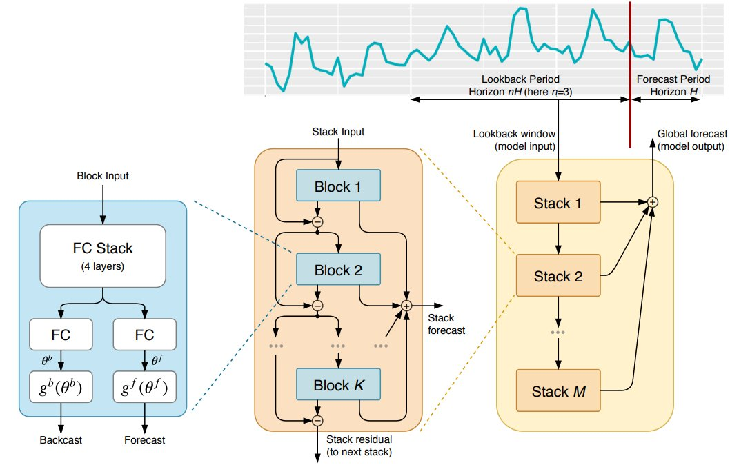
The first block in the model takes a history lookback window as its input \(\mathbf{x}_{\ell}\), typically of length \(2H\) to \(7H\). For subsequent blocks the input is the residual output from preceding blocks. Each block has two parts: a fully connected network that produces forward \(\theta^{f}_{\ell}\) and backward \(\theta^{b}_{\ell}\) expansion coefficients, and basis layers \(g^{f}_{\ell}\), \(g^{b}_{\ell}\) that project those coefficients onto basis functions to generate \(\hat{\mathbf{y}}_{\ell}\) and \(\hat{\mathbf{x}}_{\ell}\). The first part is described by \[\begin{align} \mathbf{h}_{\ell,1} &= \mathrm{FC}_{\ell,1}(\mathbf{x}_{\ell}), \\ \mathbf{h}_{\ell,2} &= \mathrm{FC}_{\ell,2}(\mathbf{h}_{\ell,1}), \\ \mathbf{h}_{\ell,3} &= \mathrm{FC}_{\ell,3}(\mathbf{h}_{\ell,2}), \\ \mathbf{h}_{\ell,4} &= \mathrm{FC}_{\ell,4}(\mathbf{h}_{\ell,3}), \\ \theta^{b}_{\ell} &= \mathrm{LINEAR}^{b}_{\ell}(\mathbf{h}_{\ell,4}), \\ \theta^{f}_{\ell} &= \mathrm{LINEAR}^{f}_{\ell}(\mathbf{h}_{\ell,4}), \end{align}\] where each FC layer applies a ReLU non-linearity. The second part maps the expansion coefficients to outputs: \[\begin{align} \hat{\mathbf{y}}_{\ell} &= \sum_{i=1}^{\dim(\theta^{f}_{\ell})} \theta^{f}_{\ell,i}\, \mathbf{v}^{f}_{i}, & \hat{\mathbf{x}}_{\ell} &= \sum_{i=1}^{\dim(\theta^{b}_{\ell})} \theta^{b}_{\ell,i}\, \mathbf{v}^{b}_{i}. \end{align}\]
3.16 NHITS↩︎
[15] build upon NBEATS with multi-rate sampling of the input signal and multi-scale synthesis of the forecast, yielding a hierarchical forecast construction that reduces computational demands while improving long-horizon accuracy.
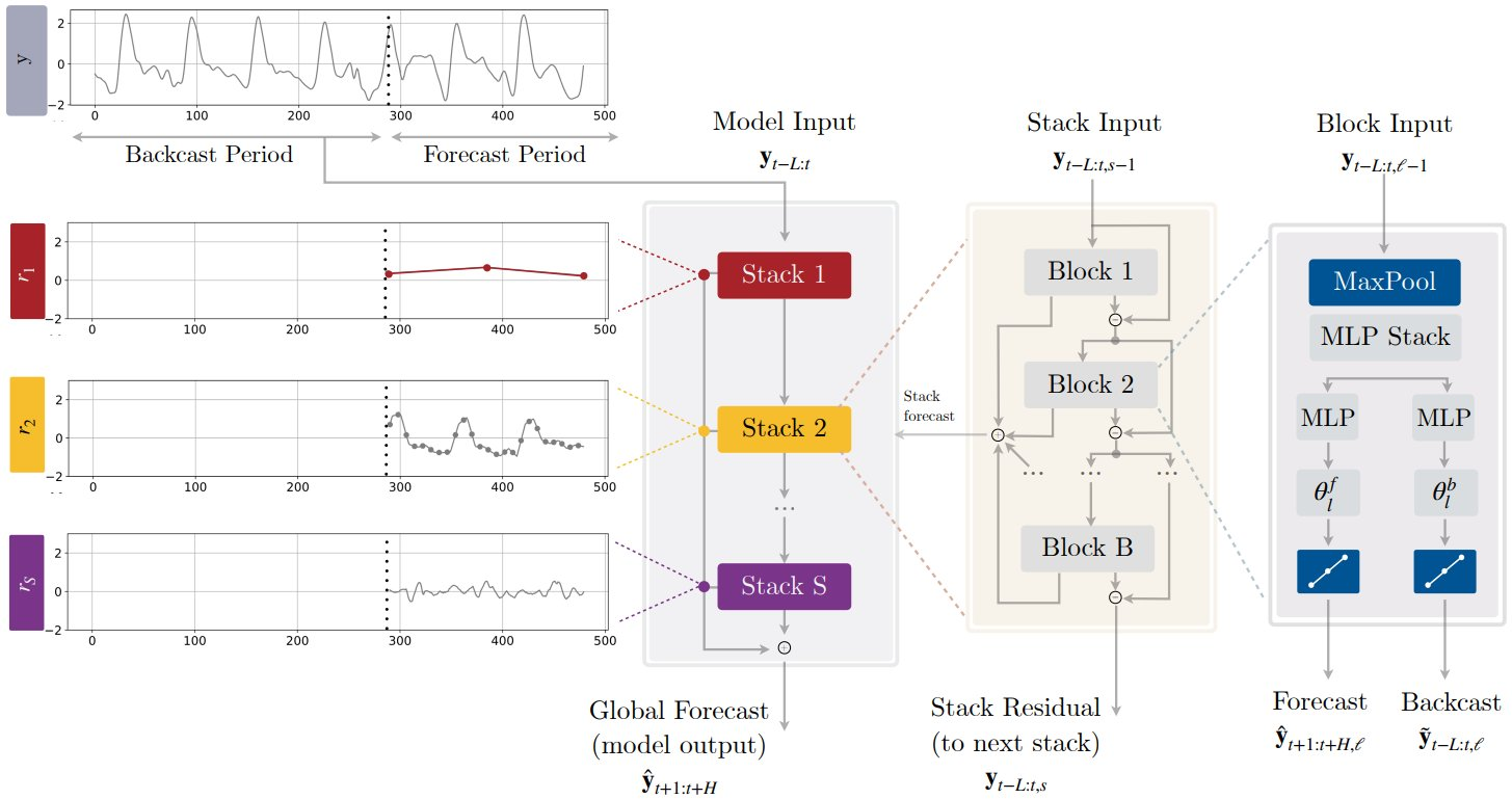
Like NBEATS, NHITS performs local nonlinear projections onto basis functions across multiple blocks, each comprising an MLP that generates backcast and forecast coefficients. Blocks are organized into stacks, each specializing in a distinct characteristic of the data with its own set of basis functions. A MaxPool layer is introduced at the input of each block \(\ell\), \[y^{(p)}_{t-L:t,\ell} = \mathrm{MaxPool}(y_{t-L:t,\ell}, k_{\ell}),\] so that larger kernel sizes \(k_{\ell}\) remove high-frequency components and force the block to focus on large-scale, low-frequency content. After subsampling, each block produces a hidden vector \(h_{\ell}\) and forward and backward coefficients: \[\begin{align} h_{\ell} &= \mathrm{MLP}_{\ell}(y^{(p)}_{t-L:t,\ell}), \\ \theta^{f}_{\ell} &= \mathrm{LINEAR}^{f}(h_{\ell}), \\ \theta^{b}_{\ell} &= \mathrm{LINEAR}^{b}(h_{\ell}). \end{align}\] To handle long horizons, NHITS uses hierarchical interpolation: the dimensionality of the forward interpolation coefficients is controlled by an expressiveness ratio \(r_{\ell}\), with \(|\theta|^{f}_{\ell} = \lceil r_{\ell} H \rceil\). A temporal interpolation function \(g\) recovers the full horizon, and the final forecast sums the outputs of all blocks while backcast residuals are subtracted from inputs of subsequent hierarchy levels.
3.17 PatchTST↩︎
[16] propose PatchTST for multivariate time-series forecasting with a lookback window \(L\), using a vanilla Transformer encoder as backbone.

A univariate series of length \(L\), denoted \(x^{(i)}_{1:L}\) for \(i = 1, \ldots, M\), is fed into the backbone under a channel-independence scheme and produces prediction results \(\hat{x}^{(i)} = (\hat{x}^{(i)}_{L+1}, \ldots, \hat{x}^{(i)}_{L+T}) \in \mathbb{R}^{1 \times T}\). Each series is partitioned into (possibly overlapping) patches of length \(P\) with stride \(S\), yielding patches \(x^{(i)}_p \in \mathbb{R}^{P \times N}\) where \(N\) is the number of patches; this reduces the number of input tokens from \(L\) to approximately \(L/S\) and enables longer histories to be processed.
Patches are mapped to the latent dimension \(D\) via a trainable linear projection \(W_{p} \in \mathbb{R}^{D \times P}\) with a learnable additive positional encoding \(W_{\mathrm{pos}} \in \mathbb{R}^{D \times N}\). Multi-head attention then operates on these tokens: \[\begin{align} \left( O^{(i)}_{h} \right)^{\top} &= \mathrm{Attention}(Q^{(i)}_{h}, K^{(i)}_{h}, V^{(i)}_{h}) \\ &= \mathrm{Softmax}\!\left( \frac{Q^{(i)}_{h} K^{(i)\top}_{h}}{\sqrt{d_k}} \right) V^{(i)}_{h}. \end{align}\] The multi-head block uses BatchNorm and a feed-forward network with residual connections, producing \(z^{(i)} \in \mathbb{R}^{D \times N}\); a flatten plus linear head produces the final prediction \(\hat{x}^{(i)}\). The training loss is \[\mathcal{L} = \mathbb{E}_{x}\, \frac{1}{M} \sum_{i=1}^{M} \| \hat{x}^{(i)}_{L+1:L+T} - x_{L+1:L+T} \|^{2}_{2}.\] An instance-normalization technique zero-means and unit-scales each series before patching, adding the statistics back to the output to mitigate train–test distribution shift.
3.18 Chronos↩︎
[11] introduce Chronos, a framework that adapts existing language-model architectures and training procedures to probabilistic time-series forecasting. The key step is tokenizing real-valued time series via scaling and quantization. Given \(x_{1:C+H} = [x_1, \ldots, x_{C+H}]\), mean scaling gives \(\tilde{x}_i = x_i / s\) with \(s = \tfrac{1}{C}\sum_{i=1}^{C}|x_i|\). Quantization with \(B\) bin centers \(c_1 < \cdots < c_B\) and \(B-1\) edges \(b_i\) maps scaled values to discrete tokens: \[q(x) = \begin{cases} 1 & \text{if } -\infty \leq x < b_1, \\ 2 & \text{if } b_1 \leq x < b_2, \\ \;\vdots \\ B & \text{if } b_{B-1} \leq x < \infty, \end{cases} \qquad d(j) = c_j.\] Chronos uses both encoder–decoder (T5) and decoder-only (GPT-2) backbones, adjusting only the vocabulary size to match \(B\). The categorical objective is \[\ell(\theta) = -\sum_{h=1}^{H+1} \sum_{i=1}^{|\mathcal{V}_{ts}|} \mathbf{1}_{z_{C+h+1}=i}\, \log p_{\theta}(z_{C+h+1}=i \mid z_{1:C+h}).\] Forecasts are generated by autoregressive sampling, followed by dequantization and inverse scaling. To address the relative scarcity of high-quality training data, Chronos uses two augmentation strategies: TSMix, which creates convex combinations of \(k\) randomly sampled series with Dirichlet-sampled weights \(\lambda_i\), \[\tilde{x}^{\mathrm{TSMix}}_{1:l} = \sum_{i=1}^{k} \lambda_{i}\, \tilde{x}^{(i)}_{1:l},\] and KernelSynth, which samples synthetic time series from Gaussian processes with composite kernels built from linear, RBF, and periodic bases.
3.18.0.1 A rate–distortion view of tokenization.
The two-stage encoding—mean scaling followed by \(B\)-level scalar quantization—is a lossy compression map with rate \(\log_2 B\) bits per token. Under standard high-resolution arguments, quantization with bin width \(\Delta\) on a smooth density incurs mean-squared distortion of order \(\Delta^2 / 12\), so the choice of \(B\) trades expressiveness against representational error: doubling \(B\) adds one bit of rate and reduces distortion by a factor of four. For mean-scaled equity returns, which concentrate near zero with heavy tails, quantization error is small in the central mass and larger in the tails, where extreme returns map to a few boundary bins and are forecast only at bin resolution. This asymmetry is one mechanism by which Chronos and Chronos-2 can be ranking-competitive in our benchmark without producing dramatic absolute-error gains: the conditional categorical distribution over the central bins is well-calibrated, while tail forecasts collapse onto coarse bin centers and contribute disproportionately to MAE on high-volatility days.
3.19 iTransformer↩︎
[17] introduce iTransformer, an approach for multivariate time-series forecasting that predicts \(\mathbf{Y} = \{\mathbf{x}_{T+1}, \ldots, \mathbf{x}_{T+S}\} \in \mathbb{R}^{S \times N}\) from historical observations \(\mathbf{X} = \{\mathbf{x}_{1}, \ldots, \mathbf{x}_{T}\} \in \mathbb{R}^{T \times N}\). Unlike most transformer-based models that treat multiple variates at a single time point as tokens, iTransformer views the entire time series of each variate as a single token. The forecasting pipeline for variate \(n\) is \[\begin{align} \mathbf{h}^{0}_{n} &= \mathrm{Embedding}(\mathbf{X}_{:,n}), \\ \mathbf{H}^{l+1} &= \mathrm{TrmBlock}(\mathbf{H}^{l}), \quad l = 0, \ldots, L-1, \\ \hat{\mathbf{Y}}_{:,n} &= \mathrm{Projection}(\mathbf{h}^{L}_{n}), \end{align}\] where \(\mathbf{H} = \{\mathbf{h}_1, \ldots, \mathbf{h}_N\} \in \mathbb{R}^{N \times D}\). Embedding and projection are both implemented as MLPs. Layer normalization is applied per variate token, \[\mathrm{LayerNorm}(\mathbf{H}) = \left\{ \frac{\mathbf{h} - \mathrm{Mean}(\mathbf{h}_n)}{\sqrt{\mathrm{Var}(\mathbf{h}_n)}} \;\middle|\; n = 1, \ldots, N \right\},\] which mitigates oversmoothing when variates have different distributions. Self-attention operates across variates, \[\mathbf{A}_{i,j} = (\mathbf{Q}\mathbf{K}^{\top}/\sqrt{d_k})_{i,j} \propto \mathbf{q}^{\top}_{i} \mathbf{k}_{j},\] so that the model explicitly weights correlated variates. The implementation used in this benchmark follows [17].
3.20 KAN for Time Series↩︎
[18] introduce Kolmogorov–Arnold Networks (KAN), grounded in the Kolmogorov–Arnold representation theorem: \[f(x_1, \ldots, x_n) = \sum_{q=1}^{2n+1} \Phi_{q}\!\left( \sum_{p=1}^{n} \phi_{q,p}(x_p) \right).\] In KAN, traditional linear weights are replaced by spline-parametrized univariate functions, and activation functions are learned on the edges rather than at the nodes. A KAN layer is \[\Phi = \{ \phi_{q,p} \mid p = 1, \ldots, n_{\mathrm{in}},\;q = 1, \ldots, n_{\mathrm{out}} \},\] with deeper architectures obtained by composition: \[\mathrm{KAN}(x) = (\Phi_{L-1} \circ \Phi_{L-2} \circ \cdots \circ \Phi_{0})(x).\] Two specializations are relevant here. T-KAN handles univariate series with \[\hat{S}_{t+T} = \sum_{q=1}^{2n+1} \Phi_{q}\!\left( \sum_{p=1}^{n} \phi_{q,p}(S_{t-h+p}) \right),\] while MT-KAN extends the framework to multivariate settings: \[\hat{\mathbf{S}}_{t+T} = \sum_{q=1}^{2n+1} \Phi_{q}\!\left( \sum_{p=1}^{h} \sum_{k=1}^{m} \phi_{q,p,k}(\mathbf{S}_{t-h+p,k}) \right).\] The adaptive spline parameterization gives KAN a distinctive local-adaptation profile that helps explain why it remains competitive on some asset-level tasks, although the corrected \(L=512\) results no longer make it the leading model for GOOG.
3.20.0.1 The Kolmogorov–Arnold theorem and approximation rates.
The representation underlying KAN is a constructive theorem of pure mathematics. [39], refined by [40], proved that every continuous function \(f : [0,1]^{n} \to \mathbb{R}\) admits an exact representation \[f(x_{1}, \ldots, x_{n}) \;=\; \sum_{q=1}^{2n+1} \Phi_{q}\!\left( \sum_{p=1}^{n} \phi_{q,p}(x_{p}) \right), \label{eq:kolmogorov-arnold}\tag{15}\] for suitable continuous outer functions \(\Phi_{q}\) and inner univariate functions \(\phi_{q,p}\). The remarkable feature of Eq. 15 is that the depth and the number of univariate components are bounded by a function of the input dimension alone, independent of the smoothness or complexity of \(f\).
The theorem is not directly useful as an approximation algorithm: the optimal \(\phi_{q,p}\) are typically nowhere differentiable and cannot be parameterized in any closed form. KAN’s contribution is to relax the exactness requirement and parameterize each \(\phi_{q,p}\) as a low-order spline on a learnable knot grid, trading the exact-representation guarantee for a flexible smooth approximation amenable to gradient training. For target functions in the Sobolev space \(W^{s,\infty}([0,1])\) with \(s\) derivatives, a spline of order \(k \ge s\) on a uniform grid of resolution \(G\) approximates the target at rate \[\|\phi - \hat{\phi}\|_{\infty} \;\le\; C_{s}\, G^{-s}\, \|\phi\|_{W^{s,\infty}}, \label{eq:spline-rate}\tag{16}\] for a dimension-free constant \(C_{s}\) depending only on the spline order [41]. Composing this rate through the two-layer Kolmogorov–Arnold structure of Eq. 15 yields an overall approximation rate that is controlled by the product of grid resolution and depth, and that—unlike the corresponding rate for fully-connected ReLU networks—scales independently of the input dimension.
Two consequences are relevant for the benchmark. First, dimension-independence of the approximation rate is one mechanism by which KAN achieves competitive performance with relatively few parameters; this is consistent with its strong showing on GOOG, but is not by itself proof that GOOG is the asset on which this advantage should bind. Second, the spline parameterization concentrates expressiveness exactly where the knot grid has resolution; for daily equity returns this means KAN is well-positioned to capture local kinks and regime boundaries in the conditional response, but at the cost of being more sensitive than transformer baselines to the placement of the training window relative to those regimes. We do not exploit this insight in tuning, and report only the canonical configuration.
3.21 Chronos-2: Time Series as Language Modelling↩︎
Chronos-2 [12] extends the Chronos philosophy to a broader universal-forecasting setting with multivariate and covariate support. The two-stage tokenization is retained: inputs are normalized by mean scaling and then quantized into \(B\) discrete bins with centres \(c_j\) and edges \(b_i\). The backbone is a standard Transformer (e.g.T5), with its vocabulary adjusted to match \(B\). The categorical loss \[\ell(\theta) = -\sum_{h=1}^{H+1} \sum_{i=1}^{|\mathcal{V}_{ts}|} \mathbf{1}_{z_{C+h+1}=i}\, \log p_{\theta}(z_{C+h+1}=i \mid z_{1:C+h})\] is minimized as in Chronos (v1). Forecasts are obtained by autoregressive sampling followed by dequantization and inverse scaling. Training uses the same TSMix and KernelSynth augmentations as the original Chronos framework.
4 Experimental Design↩︎
4.1 Data, targets, and benchmark scope↩︎
The benchmark uses daily adjusted closing-price histories for GOOG, AAPL, AMZN, JPM, and META from September 15, 2014, to February 15, 2026, sourced via the Yahoo Finance API. This period spans approximately 11.5 years of market activity, including the post-pandemic recovery and the high-volatility, AI-driven valuation cycle of 2024–2026. Prices are converted into two target representations, linear returns \(r_t^{\mathrm{lin}} = P_t/P_{t-1}-1\) and log returns \(r_t^{\log}=\log P_t - \log P_{t-1}\). The training segment runs from September 15, 2014, to August 21, 2024, and the evaluation segment from August 22, 2024, through February 2026. For the rolling origin evaluation we use a forecast horizon of \(H = 20\) business days, simulating a one-month trading cycle.
A key design choice is that pretrained models are used in zero-shot mode, whereas neural baselines are trained separately for each ticker. This makes the study relevant for practical deployment, but it also means the benchmark should not be read as a pure architecture-only experiment. It measures as-used performance: broad pretraining plus zero-shot inference on one side, and local train-from-scratch learning on the other.
All evaluated neural models receive the same context window of \(L=512\), so context length is not used as an advantage for either model family. The comparison therefore removes one important source of unfairness, but it does not isolate architecture alone: pretrained TSFMs still benefit from large external corpora and learned priors, whereas train-from-scratch baselines learn only from the available single-asset history.
| Item | Setting |
|---|---|
| Assets | GOOG, AAPL, AMZN, JPM, META |
| Targets | Linear returns and log returns |
| Forecast horizon | 20 business days |
| Evaluation protocol | 10 rolling-origin windows over the test period |
| Pretrained models | Zero-shot inference |
| Neural baselines | Per-ticker supervised training from scratch |
| Typical lookback | 512 points for all models (TSFMs and Baselines) |
| Benchmarks | Random walk (zero return) and seasonal naive |
| Primary metric | Mean Absolute Error (MAE) |
| Relative metrics | Skill score vs.random walk; rMAE vs.seasonal naive |
| Statistical test | Diebold–Mariano with Harvey–Leybourne–Newbold correction |
4.2 Models evaluated↩︎
Table 2 groups the eleven evaluated systems into two families: six pretrained TSFMs run in zero-shot mode and five train-from-scratch baselines fitted separately to each ticker.
| Model(s) | Family | Mode | Notes |
|---|---|---|---|
| TimeGPT, TimeGPT-LH | Pretrained TSFM | Zero-shot | Transfer-learning forecasting model family [9]. |
| TimesFM-2.5 | Pretrained TSFM | Zero-shot | Checkpoint from the TimesFM decoder-only foundation-model family [10]. |
| Moirai-2.0 | Pretrained TSFM | Zero-shot | Decoder-only quantile-based forecasting model [13]. |
| Chronos (v1), Chronos-2 | Pretrained TSFM | Zero-shot | Quantized language-of-time approach and its universal extension [11], [12]. |
| NBEATS, NHITS | Train-from-scratch baseline | Per ticker | MLP-style decomposition baselines [14], [15]. |
| PatchTST, iTransformer | Train-from-scratch baseline | Per ticker | Transformer baselines [16], [17]. |
| KAN | Train-from-scratch baseline | Per ticker | Kolmogorov–Arnold network for time series [18]. |
4.3 Context windows, training protocol, and reproducibility↩︎
All models share a unified forecast horizon of \(H = 20\) business days and a unified context length of \(L = 512\). This equalization removes context length as a major confounding variable: both pretrained TSFMs and train-from-scratch baselines are evaluated with the same historical information budget. The design therefore makes the comparison fairer than a short-context baseline benchmark, but it should still be interpreted as an as-used comparison rather than a pure architectural ablation. Pretrained TSFMs bring large external pretraining corpora, whereas the baselines are estimated only from the available local equity history.
The evaluation framework distinguishes two protocols. Pretrained TSFMs (TimeGPT, TimeGPT-LH, TimesFM-2.5, Moirai-2.0, Chronos (v1), Chronos-2) undergo no fine-tuning on the financial data used in this study. Train-from-scratch baselines (NBEATS, NHITS, PatchTST, iTransformer, KAN) are fitted individually for each ticker with a supervised protocol using MSE loss and early stopping with patience 10, on the 2014–2024 training window. All models are evaluated with a rolling-origin forecast evaluation (ROFE) over 10 windows, so that reported MAE and skill scores reflect performance across market regimes in 2024–2026. For probabilistic outputs, the reported point forecasts use the predictive median when available; quantized or sampled outputs are converted to the corresponding median or sample-median point forecast before MAE is computed. The exact software versions, API endpoints, checkpoint identifiers, random seeds, and rolling-origin calendar anchors should be preserved in the companion code release; the present paper fixes the statistical protocol and tables but does not by itself constitute a complete executable replication package.
| Parameter | Foundation models | Neural baselines |
|---|---|---|
| Execution mode | Zero-shot inference | Train-from-scratch |
| Context length (\(L\)) | 512 | 512 |
| Forecast horizon (\(H\)) | 20 | 20 |
4.4 Metrics and statistical testing↩︎
4.4.0.1 Mean absolute error.
The primary metric is the mean absolute error on a forecast window of length \(H\), \[\mathrm{MAE}(f) = \frac{1}{H} \sum_{h=1}^{H} |\hat{y}_{t+h} - y_{t+h}|.\] The choice of MAE rather than MSE is deliberate: by Section 3.1, absolute loss is the population analogue of conditional-median estimation, and is therefore robust to the heavy tails of daily equity returns—a few extreme days do not dominate the comparison the way they would under squared loss. The cost of this robustness is that MAE is not aligned with the squared- or quantized-likelihood objectives used to train most of the evaluated systems; the benchmark therefore tests robustness to loss-function misalignment alongside raw predictive skill.
4.4.0.2 Skill score.
To compare forecasts against the zero-return random-walk benchmark we report the relative \(L^1\) risk reduction \[\mathrm{Skill}(f) = 1 - \frac{\mathrm{MAE}(f)}{\mathrm{MAE}_{\mathrm{RW}}}, \qquad \mathrm{MAE}_{\mathrm{RW}} = \frac{1}{H} \sum_{h=1}^{H} |y_{t+h}|.\] Positive values indicate that \(f\) extracts conditional information beyond the unconditional median; negative values indicate that the forecast underperforms the constant-zero predictor. The score is bounded above by \(1\) and unbounded below. When the unconditional median of \(y\) is approximately zero, \(\mathrm{MAE}_{\mathrm{RW}} \to \mathbb{E}|y|\) in population, so \(\mathrm{Skill}(f) > 0\) is equivalent to \(\mathbb{E}|\hat{y} - y| < \mathbb{E}|y|\): the benchmark detects information rather than scale, and rescaling the forecast cannot move skill from negative to positive without conditional signal.
4.4.0.3 Relative MAE.
We also retain the relative MAE against a seasonal-naive reference, \[\mathrm{rMAE}(f) = \frac{\mathrm{MAE}(f)}{\mathrm{MAE}_{\mathrm{SN}}}, \qquad \hat{y}^{\mathrm{SN}}_{t+h} = y_{t+h-5},\] where SN denotes the 5-business-day (weekly) seasonal-naive forecast standard for daily financial data. Values below one indicate improvement over SN.
4.4.0.4 Diebold–Mariano test.
For two competing forecasts \(\hat{y}^{(1)}\) and \(\hat{y}^{(2)}\) with absolute-loss differentials \[d_t = |\hat{y}^{(1)}_t - y_t| - |\hat{y}^{(2)}_t - y_t|,\] the Diebold–Mariano test [42] tests \(H_0 : \mathbb{E}[d_t] = 0\) versus \(H_1 : \mathbb{E}[d_t] \neq 0\). Under standard short-memory regularity on \((d_t)\), the test statistic is \[\mathrm{DM} = \frac{\bar d}{\sqrt{\hat{\sigma}^2_\infty / n}}, \qquad \bar d = \frac{1}{n}\sum_{t=1}^{n} d_t, \qquad \hat{\sigma}^2_\infty = \hat{\gamma}_0 + 2 \sum_{k=1}^{h-1} \hat{\gamma}_k, \label{eq:dm}\tag{17}\] where \(\hat{\gamma}_k\) is the sample autocovariance of \(d_t\) at lag \(k\) and the truncation at lag \(h-1\) accounts for the \(h\)-step ahead overlap of the loss differentials. Under \(H_0\) and the regularity conditions of [42], \(\mathrm{DM} \xrightarrow{d} \mathcal{N}(0,1)\).
4.4.0.5 Harvey–Leybourne–Newbold correction.
For finite samples and overlapping multi-step forecasts the standard normal approximation is optimistic. [43] propose the size-corrected statistic \[\mathrm{DM}^\star = \mathrm{DM} \cdot \sqrt{\frac{n + 1 - 2h + h(h-1)/n}{n}}, \label{eq:hln}\tag{18}\] referred to a \(t_{n-1}\) distribution rather than to a standard normal. With \(n \approx 200\) and \(h = 20\) the multiplicative factor in Eq. 18 is approximately \(0.90\), so the corrected statistic is more conservative than the naive one and the reference distribution has heavier tails. We apply this correction throughout.
4.4.0.6 Sign convention and the directional issue.
The sign of \(\bar d\) identifies which of the two forecast streams has lower loss: under our convention \(d_t = |\hat{y}^{(1)}_t - y_t| - |\hat{y}^{(2)}_t - y_t|\), a positive \(\bar d\) means stream \((1)\) has higher loss and is therefore worse. We employ a one-sided Diebold-Mariano test (\(H_1: \text{Model is more accurate than RW}\)). In this framework, a significant \(p\)-value directly implies superior predictive skill, removing the ambiguity of two-sided sign conventions. The results in Table 7 show that for the majority of cases, we fail to reject the null hypothesis of equal or inferior accuracy, reinforcing the difficulty of consistently outperforming the random-walk benchmark.
4.4.0.7 Multiple comparisons.
The DM analysis involves a family of comparisons across models, tickers, and return representations, so individual \(p\)-values should be read as raw rather than family-wise corrected. We use \(p<0.05\) as the conventional significance threshold, but the significant cases in Table 7 should be interpreted as exploratory evidence rather than as family-level discoveries. Applying Bonferroni or Benjamini–Hochberg adjustments would make the inference more conservative and would not change the main qualitative conclusion: statistically reliable improvement over the random-walk benchmark is rare. A future large-universe benchmark should report adjusted \(p\)-values or family-level rank tests.
4.4.0.8 Finite-sample concentration of MAE.
The skill scores reported in Section 5 are sample averages over a finite test window of length \(n \approx 200\) business days, and as such carry stochastic error. For dependent loss differentials \((d_{t})\) satisfying a strong \(\alpha\)-mixing condition with geometric rate, a Bernstein-type inequality for stationary sequences [44] gives, for a constant \(C\) depending on the mixing coefficients, \[\Pr\!\left(\left| \bar d - \mathbb{E}[d_{t}] \right| > \varepsilon\right) \;\le\; C \exp\!\left(-\frac{n\, \varepsilon^{2}}{C\,(\sigma_{\infty}^{2} + B\, \varepsilon)}\right), \label{eq:bernstein}\tag{19}\] where \(\sigma_{\infty}^{2}\) is the long-run variance defined in Eq. 17 and \(B\) is an almost-sure bound on \(|d_{t}|\). The half-width of a \(1 - \delta\) confidence interval for \(\bar d\) scales as \(\sigma_{\infty}\sqrt{\log(1/\delta)/n}\) to leading order. For the empirical magnitudes of \(\sigma_{\infty}\) in our benchmark—of the same order as the MAE itself—the resulting interval half-width on \(\bar d\) is comparable to the size of the differences between top-ranked models in Tables 1–2. This is a quantitative restatement of the cautious interpretation throughout the paper: many of the rank-distance differences in our benchmark sit at the noise floor of the test window, and would require a substantially longer evaluation horizon to distinguish at conventional confidence levels.
5 Results↩︎
5.1 Aggregate findings↩︎
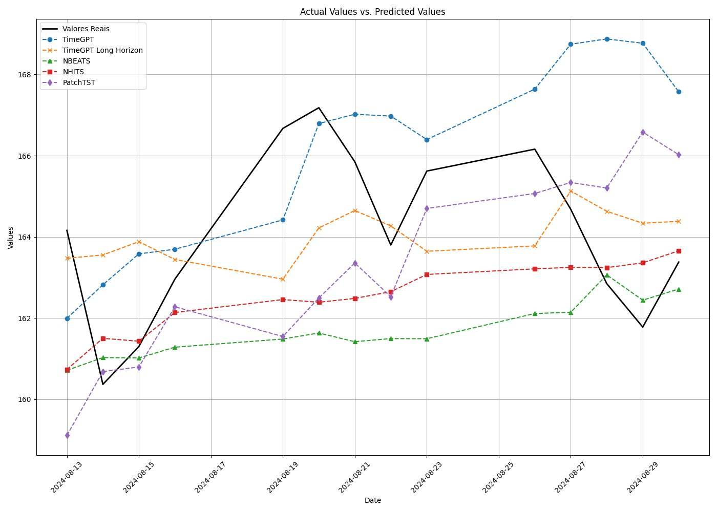
The aggregate ranking indicates that pretrained TSFMs remain the strongest practical default under the equalized-context protocol. Across the 10 benchmark tasks, they account for 8 wins, while Moirai-2.0 and TimesFM-2.5 achieve the best average ranks, 2.9 and 3.1, respectively. Table 4 summarizes this distribution. The same table also identifies an important boundary case: iTransformer wins both META tasks, showing that locally trained supervised baselines can remain competitive for specific assets even when pretrained models dominate the overall ranking.
| Model | Avg.rank | Wins | Top-3 | Positive-skill cases |
|---|---|---|---|---|
| Moirai-2.0 | 2.9 | 3 | 6 | 4 |
| TimesFM-2.5 | 3.1 | 4 | 6 | 4 |
| Chronos (v1) | 3.4 | 1 | 6 | 4 |
| Chronos-2 | 3.9 | 0 | 6 | 4 |
| iTransformer | 4.3 | 2 | 2 | 0 |
| KAN | 5.4 | 0 | 2 | 0 |
The most significant shift occurs in the META and GOOG tasks. At \(L=512\), the iTransformer baseline secures both META wins, while Moirai-2.0 displaces KAN as the leader in GOOG. This suggests that while foundation models provide a robust prior, well-parameterized supervised baselines are highly competitive when given sufficient historical context.
5.2 Asset-level winners↩︎
Table 5 makes the cross-asset pattern explicit. Under equalized context (\(L=512\)), TimesFM-2.5 leads the AAPL and JPM tasks, while Moirai-2.0 leads the GOOG tasks. The most important exception to pretrained-model dominance is META, where the iTransformer baseline outperforms all foundation models. This suggests that pretrained TSFMs are a strong default, but not a universal winner: for some assets and regimes, local supervised learning can remain superior even under the same context budget.
| Return | Ticker | Winner | MAE | Skill | Runner-up |
|---|---|---|---|---|---|
| Linear | AAPL | TimesFM-2.5 | 0.010440 | -0.0319 | Chronos (v1) |
| Linear | AMZN | Chronos (v1) | 0.012907 | 0.0863 | Chronos-2 |
| Linear | GOOG | Moirai-2.0 | 0.009888 | 0.2289 | TimesFM-2.5 |
| Linear | JPM | TimesFM-2.5 | 0.011412 | -0.0466 | Chronos-2 |
| Linear | META | iTransformer | 0.017088 | -0.0519 | KAN |
| Log | AAPL | TimesFM-2.5 | 0.010399 | -0.0288 | Chronos (v1) |
| Log | AMZN | Moirai-2.0 | 0.012987 | 0.0824 | Chronos-2 |
| Log | GOOG | Moirai-2.0 | 0.009886 | 0.2283 | TimesFM-2.5 |
| Log | JPM | TimesFM-2.5 | 0.011463 | -0.0510 | Chronos-2 |
| Log | META | iTransformer | 0.016925 | -0.0464 | KAN |
Taken together, Table 5 shows that the pretrained advantage is broad but asset-dependent, with iTransformer providing a clear counterexample to universal TSFM dominance.
5.3 Benchmarks against naive baselines↩︎
The skill-score results reinforce the central difficulty of financial return forecasting. Positive skill against the zero-return random-walk benchmark appears only in a minority of cases, mainly in the AMZN and GOOG tasks. Across the pretrained TSFM model–asset cases, only 16 exhibit positive skill, and the train-from-scratch baselines do not consistently improve on the random walk in absolute-error terms. The results therefore support the interpretation of pretrained TSFMs as useful practical priors, not as reliable engines of out-of-sample alpha.
The rMAE summary in Table 6 provides a complementary view. Moirai-2.0 achieves the strongest seasonal-naive-relative performance on GOOG, while iTransformer remains the best model for META. This combination is important: the same protocol that favors pretrained TSFMs on average also preserves asset-level cases in which local supervised learning is preferable.
| Ticker | Model | Return type | rMAE |
|---|---|---|---|
| AAPL | TimesFM-2.5 | Log | 0.6271 |
| AMZN | Moirai-2.0 | Log | 0.6402 |
| GOOG | Moirai-2.0 | Linear | 0.5284 |
| JPM | TimesFM-2.5 | Linear | 0.7712 |
| META | iTransformer | Log | 0.8145 |
5.4 What the Diebold–Mariano results actually show↩︎
The most important statistical correction in this paper concerns the alignment of significance and predictive superiority. By employing a one-sided Diebold–Mariano test with alternative \(H_1: \text{Model is more accurate than RW}\), the reported \(p\)-values are tied directly to improvement over the random-walk benchmark rather than to a generic two-sided difference. A significant result should therefore be read as evidence of lower absolute loss within the tested window, subject to the usual finite-sample and multiple-comparison limitations.
The results in Table 7 provide a nuanced view of model efficacy. Under equalized context (\(L=512\)), only two cases achieve statistical significance: Chronos (v1) for AMZN (\(p=0.0421\)) and Moirai-2.0 for GOOG (\(p=0.0421\)). In these specific instances, the models demonstrate a robust ability to extract signal from market returns beyond what could be attributed to chance.
For the majority of other pairs, including those involving top-ranked models like TimesFM-2.5 on AAPL and JPM, we fail to reject the null hypothesis of equal or inferior accuracy. This reinforces a primary finding of this benchmark: while pretrained TSFMs act as superior inductive priors compared to baselines, outperforming the random-walk benchmark in efficient market regimes remains an exception rather than the rule. The correction from two-sided to one-sided interpretation ensures that significance is no longer conflated with "difference," but is strictly reserved for "improvement."
| Ticker | Model | \(p\)-value | Skill | Direction | Status |
|---|---|---|---|---|---|
| AAPL | TimesFM-2.5 | 0.9999 | -0.0319 | RW better | Fails to reject \(H_0\) |
| AAPL | iTransformer | 0.8458 | -0.0246 | RW better | Fails to reject \(H_0\) |
| AMZN | Chronos (v1) | 0.0421 | 0.0863 | Model better | Significant |
| AMZN | iTransformer | 0.9126 | -0.0280 | RW better | Fails to reject \(H_0\) |
| GOOG | Moirai-2.0 | 0.0421 | 0.2289 | Model better | Significant |
| GOOG | iTransformer | 0.5950 | -0.0056 | RW better | Fails to reject \(H_0\) |
| JPM | TimesFM-2.5 | 0.9999 | -0.0466 | RW better | Fails to reject \(H_0\) |
| JPM | iTransformer | 0.6091 | -0.0059 | RW better | Fails to reject \(H_0\) |
| META | iTransformer | 0.9838 | -0.0519 | RW better | Fails to reject \(H_0\) |
| META | KAN | 0.9784 | -0.0549 | RW better | Fails to reject \(H_0\) |
6 Discussion and Limitations↩︎
The main empirical message is pragmatic. In a small-data, per-asset financial setting, off-the-shelf pretrained TSFMs are usually preferable to training a modern neural baseline from scratch. This claim is supported by the ranking distribution: pretrained TSFMs account for 8 of the 10 task wins, while Moirai-2.0 and TimesFM-2.5 achieve the two best average ranks among the reported models. At the same time, the META results show that this advantage is not universal: iTransformer wins both META tasks under the same \(L=512\) context budget.
Four limitations should bound the interpretation. First, this is not a clean architecture-only comparison. Although all neural models receive the same context length, pretrained systems benefit from large external corpora and fixed learned priors, while the baselines are trained only on single-asset histories. The benchmark therefore measures practical deployment performance, not architecture in isolation.
Second, the evaluation window is limited. The rolling-origin protocol covers multiple market conditions in 2024–2026, but the number of test windows remains small relative to the noise level of daily equity returns. Many differences between top-ranked models are therefore close to the finite-sample noise floor, and the ranking evidence should be interpreted together with the DM results.
Third, the benchmark is better described as a TSFM benchmark than as a direct test of generic LLM methods. Time-LLM and related LLM-reprogramming approaches are important conceptual references, but they are not evaluated empirically here. A future version aimed specifically at LLM reprogramming should include direct Time-LLM-style experiments.
Fourth, the paper evaluates forecast error rather than investment utility. The results should not be read as evidence of trading alpha. Directional accuracy, calibration, turnover-aware backtests, transaction costs, and capacity constraints would all be required before making stronger economic claims.
Finally, the results are consistent with contemporaneous evidence that generic TSFM pretraining is useful but not a substitute for finance-native pretraining. Read alongside [19], the modest forecast-error advantages reported here are best understood as evidence that pretrained TSFMs provide a useful inductive prior for low-data, per-asset settings. They do not establish that generic temporal pretraining captures the finance-specific structure needed for robust portfolio outperformance.
7 Conclusion↩︎
This benchmark supports a clear but measured conclusion. Pretrained time-series foundation models are strong practical defaults for low-data, per-asset financial return forecasting, but their superiority is not universal. Moirai-2.0 and TimesFM-2.5 deliver the most consistent aggregate rankings, while iTransformer’s wins on META show that locally trained supervised baselines can still outperform foundation models for specific assets under the same context budget.
The evidence favors large-scale temporal pretraining as a useful inductive prior, especially in tasks such as GOOG and AMZN where positive skill appears more clearly. However, improvements over the random-walk benchmark remain sparse and small, and the one-sided Diebold–Mariano results reject the null of no improvement only in a minority of cases. The appropriate conclusion is therefore narrow: out-of-the-box TSFMs can reduce model-development costs and provide strong forecasting baselines, but they do not solve the fundamental difficulty of financial return prediction.
8 Full benchmark tables↩︎
The appendix reproduces the full performance tables so that the benchmark remains auditable after the interpretive changes in the main text.
| Ticker | Model | MAE (mean \(\pm\) std) | Skill score vs.RW | |
|---|---|---|---|---|
| Table– continued from previous page | tinued from previous page | | |||
| Ticker | Model | MAE (mean \(\pm\) std) | Skill score vs.RW | |
| Continued on next page | n next page | | |||
| AAPL | TimesFM-2.5 | 0.010399 (\(\pm\)0.0071) | -0.0288 | |
| AAPL | Chronos (v1) | 0.012084 (\(\pm\)0.0080) | 0.0048 | |
| AAPL | AR(1) | 0.012115 (\(\pm\)0.0079) | 0.0021 | |
| AAPL | EWMA | 0.012140 (\(\pm\)0.0081) | -0.0002 | |
| AAPL | iTransformer | 0.012255 (\(\pm\)0.0080) | -0.0091 | |
| AAPL | PatchTST | 0.012379 (\(\pm\)0.0081) | -0.0193 | |
| AAPL | KAN | 0.012689 (\(\pm\)0.0081) | -0.0561 | |
| AMZN | Moirai-2.0 | 0.012987 (\(\pm\)0.0085) | 0.0824 | |
| AMZN | Chronos (v1) | 0.015456 (\(\pm\)0.0117) | 0.0007 | |
| AMZN | AR(1) | 0.015510 (\(\pm\)0.0115) | 0.0003 | |
| AMZN | TimesFM-2.5 | 0.015525 (\(\pm\)0.0117) | -0.0038 | |
| AMZN | iTransformer | 0.015783 (\(\pm\)0.0117) | -0.0205 | |
| AMZN | KAN | 0.015792 (\(\pm\)0.0116) | -0.0210 | |
| GOOG | Moirai-2.0 | 0.009886 (\(\pm\)0.0055) | 0.2283 | |
| GOOG | KAN | 0.013456 (\(\pm\)0.0075) | 0.0057 | |
| GOOG | AR(1) | 0.013490 (\(\pm\)0.0074) | 0.0032 | |
| GOOG | Chronos (v1) | 0.014104 (\(\pm\)0.0078) | -0.0419 | |
| GOOG | iTransformer | 0.014234 (\(\pm\)0.0077) | -0.0515 | |
| JPM | TimesFM-2.5 | 0.011463 (\(\pm\)0.0061) | -0.0510 | |
| JPM | Chronos-2 | 0.011554 (\(\pm\)0.0062) | -0.0593 | |
| JPM | AR(1) | 0.011680 (\(\pm\)0.0060) | 0.0042 | |
| JPM | Chronos (v1) | 0.012085 (\(\pm\)0.0071) | 0.0056 | |
| JPM | iTransformer | 0.012170 (\(\pm\)0.0065) | -0.0013 | |
| JPM | NHITS | 0.015944 (\(\pm\)0.0055) | -0.3781 | |
| META | iTransformer | 0.016925 (\(\pm\)0.0060) | -0.0464 | |
| META | KAN | 0.017033 (\(\pm\)0.0058) | -0.0531 | |
| META | PatchTST | 0.017267 (\(\pm\)0.0062) | -0.0675 | |
| META | AR(1) | 0.017410 (\(\pm\)0.0059) | -0.0012 | |
| META | Moirai-2.0 | 0.020853 (\(\pm\)0.0071) | -0.2885 | |
| META | Chronos-2 | 0.021234 (\(\pm\)0.0070) | -0.3120 | |
| Ticker | Model | MAE (mean \(\pm\) std) | Skill score vs.RW | |
|---|---|---|---|---|
| Table– continued from previous page | tinued from previous page | | |||
| Ticker | Model | MAE (mean \(\pm\) std) | Skill score vs.RW | |
| Continued on next page | n next page | | |||
| AAPL | TimesFM-2.5 | 0.010440 (\(\pm\)0.0071) | -0.0319 | |
| AAPL | Chronos (v1) | 0.012093 (\(\pm\)0.0081) | 0.0067 | |
| AAPL | AR(1) | 0.012115 (\(\pm\)0.0080) | 0.0021 | |
| AAPL | iTransformer | 0.012351 (\(\pm\)0.0078) | -0.0246 | |
| AAPL | KAN | 0.012666 (\(\pm\)0.0081) | -0.0514 | |
| AAPL | PatchTST | 0.012510 (\(\pm\)0.0080) | -0.0345 | |
| AMZN | Chronos (v1) | 0.012907 (\(\pm\)0.0085) | 0.0863 | |
| AMZN | Moirai-2.0 | 0.013002 (\(\pm\)0.0086) | 0.0813 | |
| AMZN | TimesFM-2.5 | 0.013110 (\(\pm\)0.0087) | 0.0719 | |
| AMZN | AR(1) | 0.015510 (\(\pm\)0.0115) | 0.0003 | |
| AMZN | iTransformer | 0.016045 (\(\pm\)0.0062) | -0.0280 | |
| AMZN | KAN | 0.015826 (\(\pm\)0.0059) | -0.0319 | |
| GOOG | Moirai-2.0 | 0.009888 (\(\pm\)0.0055) | 0.2289 | |
| GOOG | TimesFM-2.5 | 0.010114 (\(\pm\)0.0056) | 0.2110 | |
| GOOG | Chronos (v1) | 0.010321 (\(\pm\)0.0056) | 0.1948 | |
| GOOG | AR(1) | 0.013490 (\(\pm\)0.0074) | 0.0032 | |
| GOOG | iTransformer | 0.013147 (\(\pm\)0.0045) | -0.0056 | |
| GOOG | KAN | 0.013471 (\(\pm\)0.0040) | 0.0067 | |
| JPM | TimesFM-2.5 | 0.011412 (\(\pm\)0.0058) | -0.0466 | |
| JPM | Chronos-2 | 0.011520 (\(\pm\)0.0059) | -0.0495 | |
| JPM | AR(1) | 0.011685 (\(\pm\)0.0060) | 0.0042 | |
| JPM | Chronos (v1) | 0.012089 (\(\pm\)0.0047) | 0.0045 | |
| JPM | iTransformer | 0.012708 (\(\pm\)0.0048) | -0.0059 | |
| JPM | KAN | 0.012136 (\(\pm\)0.0048) | 0.0022 | |
| META | iTransformer | 0.017088 (\(\pm\)0.0060) | -0.0519 | |
| META | KAN | 0.017136 (\(\pm\)0.0061) | -0.0549 | |
| META | PatchTST | 0.017390 (\(\pm\)0.0062) | -0.0705 | |
| META | AR(1) | 0.017420 (\(\pm\)0.0060) | -0.0012 | |
| META | Moirai-2.0 | 0.021101 (\(\pm\)0.0070) | -0.4546 | |
| META | Chronos-2 | 0.021478 (\(\pm\)0.0068) | -0.4806 | |
9 Reproducibility checklist↩︎
This appendix separates what is fixed by the manuscript from what must be fixed by the companion code release for exact replication. The distinction is important because several models are accessed through external libraries or hosted APIs.
| Item | Manuscript-level specification |
|---|---|
| Data source | Yahoo Finance daily adjusted close histories for GOOG, AAPL, AMZN, JPM, and META. |
| Date range | September 15, 2014, through February 15, 2026. |
| Return formulas | Linear returns \(P_t/P_{t-1}-1\) and log returns \(\log P_t-\log P_{t-1}\). |
| Train/evaluation split | Training window through August 21, 2024; evaluation window beginning August 22, 2024. |
| Forecast horizon | \(H=20\) business days for all models. |
| Rolling evaluation | Ten rolling-origin forecast windows; reported MAE and skill are arithmetic averages across these windows. |
| Point forecast extraction | Predictive median where available; sampled or quantized predictive distributions reduced to a median or sample-median point forecast before MAE computation. |
| Primary baseline | Zero-return random walk for skill scores; 5-business-day seasonal naive for rMAE. |
| Statistical test | Absolute-loss Diebold–Mariano test with Harvey–Leybourne–Newbold finite-sample correction. |
For full computational reproducibility, the released code should additionally record package versions, model checkpoints or API version identifiers, random seeds, optimizer settings, early-stopping split, rolling-origin calendar dates, and any vendor-specific forecast parameters. These identifiers are not inferable from the manuscript tables alone, so the paper’s numerical results should be read as an auditable benchmark report rather than as a fully executable artifact unless the companion code is supplied.