A geometric multimessenger consistency test of radiative and near-zone gravity with LISA and SKA
June 25, 2026
Abstract
Compact binary pulsars observed both through precision radio timing and low-frequency gravitational waves offer a direct way to compare the same binary geometry with two independent messengers. We propose a multimessenger consistency test based on the orbital inclination, measured from the Shapiro-delay shape parameter in radio timing and from the tensor polarization amplitude ratio in the gravitational-wave signal. Defining the common-epoch residual \(\varepsilon(t_0)=s_{\rm Shapiro}(t_0)-s_{\rm GW}(t_0)\), general relativity predicts \(\varepsilon=0\), while a nonzero value would indicate either an unmodeled systematic or a mismatch between the near-zone and radiative descriptions of gravity. We estimate the attainable precision on this quantity for representative LISA–SKA compact binary pulsars using a seven-parameter timing Fisher matrix and a sky-averaged LISA sensitivity curve including the Galactic foreground. We adopt a conservative radio baseline, \(\sigma_{\rm TOA}=1\,\mu{\rm s}\) and \(N_{\rm eff}=10^4\), intended to summarize radiometer noise, jitter, residual dispersion-measure and scattering effects, profile evolution, and cadence losses after wideband timing. For systems at \(d=5\,{\rm kpc}\) observed for four years, we find \(\sigma_\varepsilon\simeq4\times10^{-3}\) for a favorable double neutron star and \(\sigma_\varepsilon\simeq9\times10^{-4}\) for a hypothetical pulsar–black-hole system. The former is the more robust astrophysical benchmark; the latter illustrates the reach if such a high-SNR chirping source is discovered. The useful cases remain limited mainly by gravitational-wave polarimetry, while radio timing supplies the near-zone reference measurement of the inclination. These results define a quantitative target for future joint Bayesian analyses of compact binary pulsars observed in both radio and gravitational waves.
1 Introduction↩︎
Binary pulsars provide some of the most precise tests of gravity currently available. Radio timing probes the near-zone spacetime through pulse propagation effects, orbital dynamics, and post-Keplerian timing parameters [1]–[5]. The coming low-frequency gravitational-wave era adds a complementary view of the same systems. A subset of compact binary pulsars, especially short-period Galactic double neutron stars and possible pulsar–black-hole systems, should be observable both as radio pulsars timed with SKA-class precision and as slowly evolving low-frequency sources in LISA-like detectors [6]–[8]. LISA studies of Galactic binaries, verification binaries, and time-delay interferometry have already established the detector-response language needed to discuss such systems [9]–[13]. This opens up a multimessenger problem that is more interesting than parameter combination alone: the same binary geometry can be measured in two physically distinct ways.
In this paper we focus on the orbital inclination \(\iota\). In the gravitational-wave channel, \(\iota\) is inferred from the polarization content of the radiative field. In the radio channel, \(s=\sin\iota\) is inferred from the Shapiro delay experienced by pulses propagating through the companion’s gravitational potential. In general relativity these are simply different functions of the same angle. More generally they need not agree. A non-tensor contribution can bias the tensor-only polarization ratio used in the GW analysis, while a modified near-zone metric can bias the Shapiro-delay shape. The equality between \(s_{\rm GW}\) and \(s_{\rm Shapiro}\) is therefore a geometric cross-check between the radiative and near-zone sectors of the theory.
The point is not that this test outperforms every existing binary-pulsar bound. It does not. The strongest scalar-tensor constraints from systems such as PSR J1738+0333 and the double pulsar rely on dipole-radiation and orbital-damping channels [3], [4]. The observable studied here probes something different: whether the inclination inferred from the radiative polarization geometry agrees with the inclination inferred from the near-zone metric. In that sense it is complementary to the usual \(\dot{P}_b\) tests, just as polarization, propagation, and generation tests are complementary within the broader GW tests-of-GR program [5], [14]–[16].
The credibility of this comparison depends on several practical issues. On the timing side, the Shapiro Fisher matrix must include the Roemer covariance and should be separated cleanly from assumptions about cadence and the effective amount of independent information. On the gravitational-wave side, the polarimetric inclination estimate must be used with due care, since it is only an analytic approximation to a full LISA inference problem. The Galactic foreground is anisotropic, and non-contemporaneous observations may be affected by secular changes in the projected orbit. Our aim here is to keep these issues explicit while still working with an analytic calculation that makes the basic scaling of the observable transparent.
The paper is organized as follows. Section 2 places the observable in the context of existing binary-pulsar and GW tests. Section 3 defines the radiative and near-zone inclination measurements and the common-epoch residual. Section 4 discusses phenomenological non-tensor leakage and the associated phase-coherence caveat. Section 5 develops the timing Fisher matrix, explains the treatment of cadence and effective timing weight, and summarizes omitted timing terms such as the Einstein delay. Section 6 describes the LISA estimate and the way we bracket its unmodeled covariance. Section 7 presents the benchmark results. Section 8 discusses cadence, Galactic confusion, chirping, precession, and common-epoch modeling. Section 9 reports algebraic and numerical checks. Section 10 explains how the observable should be interpreted in specific theories, and Sec. 11 outlines the corresponding Bayesian analysis. Appendices summarize the Takahashi–Seto scaling used here, the circular Shapiro identity, the seven-parameter timing derivatives, and reproducibility details. We use \(G=c=1\) in analytic formulae unless SI units are displayed.
2 Relation to existing binary-pulsar and GW tests↩︎
It is useful to separate three types of tests that are often grouped together. The first class consists of timing-only post-Keplerian tests. In those tests one measures several timing parameters, such as periastron advance, Einstein delay, Shapiro range and shape, and orbital decay, and asks whether a single pair of masses in a specified theory explains them. The second class consists of radiative tests, where the waveform phase, polarization, or propagation is compared with GR. The third class, to which the present paper belongs, compares two operational definitions of the same source geometry obtained from different sectors of the field. The inclination residual is not a stronger version of \(\dot{P}_b\); it is a different null relation.
This distinction matters for interpreting numerical reach. A scalar-tensor theory with a light scalar can generate dipole radiation that is strongly constrained by \(\dot{P}_b\). The same theory may generate much smaller changes in the tensor polarization ratio for a given binary orientation. It would therefore be misleading to rank the present observable solely by whether it improves the best scalar-tensor coupling bound. Its value is that it tests whether the radiative field and the near-zone metric encode the same inclination. This is the same logic that makes polarization tests interesting even when phase tests give stronger bounds in a specific model: the two observables probe different projections of theory space.
The observable is also distinct from ordinary LISA–radio parameter combination. A joint fit that assumes GR will return a better common inclination, Eq. 10 . A null test instead asks whether the two inclination estimates are mutually consistent before imposing the equality. In a data-analysis implementation, one would therefore run at least two fits: a GR-constrained joint fit with a common \(\iota\), and a consistency fit with independent \(s_{\rm Shapiro}\) and \(s_{\rm GW}\). The residual \(\varepsilon\) is the difference between the two independently inferred quantities in the latter fit.
3 The geometric observable↩︎
3.1 Radiative inclination from GW polarimetry↩︎
For a slowly evolving compact binary in the LISA band, the leading tensor quadrupole waveform can be written, in the standard transverse-traceless convention, as \[\begin{align} h_+(t) &= A_0(1+\cos^2\iota)\cos\Phi(t),\tag{1}\\ h_\times(t) &= 2A_0\cos\iota\sin\Phi(t),\tag{2} \end{align}\] where \(A_0\) absorbs the conventional factor \(2(\pi f\mathcal{M})^{2/3}\mathcal{M}/d\) and any detector-response normalization. The SNR calculation below uses the standard sky-averaged LISA sensitivity curve, so no additional response factor is applied to Eqs. 1 –2 . Here \(\mathcal{M}\) is the chirp mass, \(f=2/P_b\) for the dominant harmonic, and \(d\) is the distance. The tensor polarization amplitude ratio is \[\mathcal{R}_{\rm GW}\equiv \frac{A_\times}{A_+}=\frac{2\cos\iota}{1+\cos^2\iota}. \label{eq:rgw}\tag{3}\] It is independent of \(\mathcal{M}\), \(d\), and \(f\) at this order. On the branch \(0\leq \iota\leq \pi/2\), the inverse is \[\cos\iota_{\rm GW}(\mathcal{R}_{\rm GW})=\frac{1-\sqrt{1-\mathcal{R}_{\rm GW}^2}}{\mathcal{R}_{\rm GW}}, \label{eq:inv}\tag{4}\] with the edge-on limit taken by continuity. We define \[s_{\rm GW}=\sqrt{1-\cos^2\iota_{\rm GW}}.\] The reflection ambiguity between \(\iota\) and \(\pi-\iota\) is less dangerous for this particular observable than for many inclination measurements, because \(s=\sin\iota\) is branch-invariant. A practical LISA analysis may still sample both signs of \(\cos\iota\) because the polarization phase and orbital ephemeris can carry sign information, but both branches are mapped to the same \(s_{\rm GW}\) before forming \(\varepsilon\). Thus the ordinary inclination-reflection degeneracy does not by itself generate a bimodal \(\varepsilon\) posterior; only effects that break the simple tensor-ratio symmetry, such as a response-dependent non-tensor leakage, would require branch-specific interpretation.
3.2 Near-zone inclination from the Shapiro delay↩︎
In the Damour–Taylor parametrization, the Shapiro delay for a binary pulsar is [1] \[\Delta_S(u)=-2r\ln A(u),\qquad A(u)=1-e\cos u-sq(u), \label{eq:shapiro}\tag{5}\] where \(r=Gm_c/c^3\), \(s=\sin\iota\), \(u\) is the eccentric anomaly, \(e\) is the eccentricity, and \[q(u)=\sin\omega(\cos u-e)+\sqrt{1-e^2}\cos\omega\sin u. \label{eq:q}\tag{6}\] The corresponding Roemer delay is \[\Delta_R(u)=xq(u), \label{eq:roemer}\tag{7}\] where \(x=a_p\sin\iota/c\) is the projected semimajor axis of the pulsar orbit. In what follows \(s_{\rm Shapiro}\) means the marginalized posterior for the Shapiro shape parameter obtained from a global radio timing model. It is not a direct measurement of \(s\) in isolation: real fits include Roemer, Shapiro, Einstein, secular, propagation, and instrumental terms. The simplified Fisher block used here isolates the local information carried by the Roemer–Shapiro shape after the long-term timing solution has constrained the remaining orbital geometry.
3.3 Cross-messenger residual↩︎
The null residual is a common-epoch quantity, \[\varepsilon(t_0)\equiv s_{\rm Shapiro}(t_0)-s_{\rm GW}(t_0;\mathcal{R}_{\rm GW}). \label{eq:eps}\tag{8}\] The epoch \(t_0\) is a source-frame orbital reference epoch propagated consistently through the radio and GW ephemerides; the common light-travel time to the Solar System barycenter cancels because both messengers originate from the same binary. If the radio and LISA data are not contemporaneous, or if the orbital plane precesses, both posteriors must be transported to \(t_0\) under a shared orientation model before Eq. 8 is interpreted. In GR, and in the absence of unmodeled systematics, \(\varepsilon(t_0)=0\). Linear propagation gives \[\sigma_\varepsilon^2=(\sigma_s^{\rm Shapiro})^2+\cos^2\iota\,(\sigma_\iota^{\rm LISA})^2, \label{eq:sigeps}\tag{9}\] where the two channels are independent. The same data also give a joint estimate of the common inclination, \[\frac{1}{(\sigma_\iota^{\rm joint})^2}=\frac{1}{(\sigma_\iota^{\rm LISA})^2}+\frac{\cos^2\iota}{(\sigma_s^{\rm Shapiro})^2}. \label{eq:joint}\tag{10}\] Equations 9 and 10 answer different questions. The former is the threshold for detecting a disagreement; the latter is the precision on \(\iota\) if GR is assumed.
4 Non-tensor polarizations and near-zone biases↩︎
The observable is most cleanly defined without committing to a specific modified-gravity Lagrangian. For interpretation, however, it is useful to write down how a generic non-tensor sector enters. Let the strain measured by a LISA channel \(I\) be \[h_I=F_I^+ h_+ + F_I^\times h_\times + \sum_A F_I^A h_A, \label{eq:response95modes}\tag{11}\] where \(A\) runs over possible breathing, longitudinal, and vector modes [15], [16]. In a tensor-only analysis the additional terms are absorbed into effective plus and cross amplitudes. To leading order this can be written as \[\begin{align} A_+^{\rm eff} &= A_+(1+\delta_+),\; A_\times^{\rm eff} &= A_\times(1+\delta_\times), \end{align}\] where \(\delta_+\) and \(\delta_\times\) are not fundamental constants; they depend on sky position, polarization angle, detector response, source orientation, and the amplitudes of the extra modes. The observed ratio becomes \[\mathcal{R}_{\rm GW}^{\rm obs}=\mathcal{R}_{\rm GW}^{\rm GR}\left[1+\delta_\times-\delta_+ +O(\delta^2)\right]. \label{eq:deltaR}\tag{12}\] Since \[\frac{\mathrm{d}s}{\mathrm{d}\mathcal{R}_{\rm GW}}=-\frac{\cos\iota(1+\cos^2\iota)^2}{2\sin^3\iota}, \label{eq:dsdR}\tag{13}\] up to the sign convention for the inclination branch, the induced radiative contribution to the residual is approximately \[\varepsilon_{\rm rad}\simeq -\frac{\mathrm{d}s}{\mathrm{d}\mathcal{R}_{\rm GW}}\,\mathcal{R}_{\rm GW}\,(\delta_\times-\delta_+). \label{eq:epsrad}\tag{14}\] A near-zone modification may similarly bias the Shapiro shape. If the timing model returns \(s_{\rm Shapiro}=s+\delta s_{\rm NZ}\), then \[\varepsilon\simeq \delta s_{\rm NZ}+\varepsilon_{\rm rad}. \label{eq:eps95decomp}\tag{15}\] A useful order-of-magnitude calibration follows immediately from Eq. 14 . At the fiducial inclination \(\iota=65^\circ\), \(\mathcal{R}_{\rm GW}=0.717\) and \(|\mathrm{d}s/\mathrm{d}\mathcal{R}_{\rm GW}|=0.394\), so \[|\varepsilon_{\rm rad}|\simeq 0.28\,|\delta_\times-\delta_+|. \label{eq:nontensor95example}\tag{16}\] If a breathing-mode amplitude \(A_b\) leaks into a tensor-only fit with an effective projection coefficient \(\eta_b\) such that \(\delta_\times-\delta_+\simeq \eta_b A_b/A_T\), the DNS baseline sensitivity \(\sigma_\varepsilon\simeq4.1\times10^{-3}\) corresponds to a fractional leakage \(A_b/A_T\sim1.5\times10^{-2}\eta_b^{-1}\), while the PSR+BH reach value corresponds to \(\sim3\times10^{-3}\eta_b^{-1}\). This is not a theory-parameter bound; it only translates the observable into the size of a tensor-amplitude bias. In scalar-tensor binaries, quadrupolar scalar amplitudes can be suppressed by powers of the orbital velocity, while dipole radiation can instead dominate the phase evolution. Therefore there are two regimes: if phase dephasing is large, a phase test will detect the inconsistency before Eq. 14 is meaningful; if the signal is phase coherent but has small response-dependent polarization leakage, \(\varepsilon\) provides an independent amplitude-geometry check.
This decomposition is the main theoretical point. Following the conservative choice adopted here, we do not build a toy scalar-tensor exclusion map. The test is a clean residual, but its interpretation is deliberately phenomenological until one supplies a theory-specific waveform and a near-zone metric. We therefore quote sensitivities in \(\sigma_\varepsilon\), not as exclusion contours in a surrogate scalar-tensor parameter plane. A faithful Damour–Esposito–Farese interpretation would require scalarized stellar structure, modified radiative polarizations, and a LISA response fit; that is beyond the present forecasting paper [17], [18].
There is also a phase-coherence caveat. Many theories that generate scalar or vector radiation also change the phase evolution, for instance through dipole radiation. If such dephasing is large over the LISA observation, a strictly GR extraction template would fail before the polarization-ratio test is applied. The amplitude-bias description above therefore assumes either that the signal remains phase coherent under the extraction template, or that \(A_+\) and \(A_\times\) are measured using a theory-agnostic or theory-specific phase model. In a real analysis, a large phase inconsistency would be a separate detection channel, and the residual \(\varepsilon\) should be evaluated only after a waveform model capable of coherently extracting the polarizations has been specified.
5 Timing Fisher analysis↩︎
5.1 Seven-parameter timing Fisher matrix↩︎
The timing observable used in the Fisher matrix is \[\Delta(u)=\Delta_R(u)+\Delta_S(u)=xq(u)-2r\ln A(u). \label{eq:total95delay}\tag{17}\] For the fiducial forecasts we use the seven-parameter vector \[\boldsymbol{\theta}=(s,r,x,P_b,T_0,e,\omega).\] The parameters \(e\) and \(\omega\) are therefore included explicitly in the local Fisher matrix, with modest Gaussian priors representing information from the long-term timing solution. Our default prior widths are \[\sigma_e=10^{-4},\qquad \sigma_\omega=10^{-3}\, {\rm rad}. \label{eq:eomega95priors}\tag{18}\] These priors are not meant to replace a global timing analysis. They simply prevent the short local Roemer–Shapiro block from being asked to determine the full eccentric geometry by itself, which is not how a real compact-binary timing solution is obtained. The seven-parameter derivatives are given in Appendix 15 and are used for the production values in Tables ¿tbl:tab:forecast? and ¿tbl:tab:timing95robust?. A five-parameter block is retained only as a diagnostic comparison. The results remain conditional on a timing solution that tracks the secular eccentric geometry, in particular \(\omega(t)\), over the observing span.
Let \[M=\frac{2\pi(t-T_0)}{P_b},\qquad u-e\sin u=M,\] so that \[\frac{\partial u}{\partial P_b}=-\frac{M}{P_b(1-e\cos u)},\qquad \frac{\partial u}{\partial T_0}=-\frac{2\pi}{P_b(1-e\cos u)}. \label{eq:du}\tag{19}\] Writing \[\dot{q}\equiv\frac{\partial q}{\partial u}=-\sin\omega\sin u+\sqrt{1-e^2}\cos\omega\cos u, \label{eq:qdot}\tag{20}\] we obtain the partial derivatives used in the body of the calculation: \[\begin{align} \frac{\partial\Delta}{\partial s} &= \frac{2rq}{A}, \tag{21}\\ \frac{\partial\Delta}{\partial r} &= -2\ln A,\tag{22}\\ \frac{\partial\Delta}{\partial x} &= q,\tag{23}\\ \frac{\partial\Delta}{\partial u} &= x\dot{q}+\frac{2r}{A}\left(s\dot{q}-e\sin u\right),\tag{24}\\ \frac{\partial\Delta}{\partial P_b} &= \frac{\partial\Delta}{\partial u}\left[-\frac{M}{P_b(1-e\cos u)}\right],\tag{25}\\ \frac{\partial\Delta}{\partial T_0} &= \frac{\partial\Delta}{\partial u}\left[-\frac{2\pi}{P_b(1-e\cos u)}\right].\tag{26} \end{align}\] The sign in Eq. 24 is worth noting: \(\partial_u[-2r\ln A]=-(2r/A)\partial_u A=(2r/A)(s\dot{q}-e\sin u)\).
The Fisher matrix is evaluated as \[\Gamma_{ij}=\sum_{k=1}^{N_{\rm samp}}\frac{1}{\sigma_{\rm TOA}^2} \frac{\partial\Delta(t_k)}{\partial\theta_i} \frac{\partial\Delta(t_k)}{\partial\theta_j}w, \label{eq:fisher}\tag{27}\] where \(w=N_{\rm eff}/N_{\rm samp}\) rescales the dense numerical grid to the assumed effective number of statistically independent timing measurements. Our baseline uses \[N_{\rm eff}=10^4,\qquad T_{\rm obs}=4~{\rm yr},\qquad \sigma_{\rm TOA}=1~\mu{\rm s}, \label{eq:sampling}\tag{28}\] and Fig. 4 scans \(N_{\rm eff}=10^3,10^4,10^5\). As a rough physical anchor, \(N_{\rm eff}=10^4\) may be thought of as a multi-year campaign with a few hundred useful observing epochs and tens of effectively independent orbital-phase measurements per epoch after folding, de-dispersion, and profile-domain compression. It is an information weight, not a literal count of individual pulses. The earlier shorthand \(20T_{\rm obs}/P_b\) is useful only as a phase-quadrature scale and is not interpreted here as a continuous-observing schedule.
The adopted \(1\,\mu{\rm s}\) value is deliberately more conservative than the \(\sim100\,{\rm ns}\) precision achievable for the best bright millisecond pulsars. A compact PSR+BH at several kpc need not be such an ideal timing source. The radio flux decreases as \(d^{-2}\), while the integration time needed to reach a fixed radiometer-limited TOA precision scales roughly as \(d^4\). Residual dispersion-measure variations, scattering, scintillation, pulse jitter, profile evolution, calibration errors, and imperfect wideband template modeling then enter the effective timing covariance rather than the binary Shapiro formula itself [19]–[22]. In the compressed Fisher calculation we summarize these effects by \[\sigma_{\rm TOA}^2=\sigma_{\rm rad}^2+\sigma_{\rm jitter}^2+\sigma_{\rm DM}^2+\sigma_{\rm scatt}^2+\sigma_{\rm prof}^2+\cdots, \label{eq:sigma95toa95budget}\tag{29}\] and by reducing the raw number of phase samples to \(N_{\rm eff}\). In a full analysis one should instead use the complete covariance, \[\Gamma_{ij}=\partial_i\boldsymbol{\Delta}^T C^{-1}\partial_j\boldsymbol{\Delta},\] where \(C\) contains white, chromatic, profile-domain, and correlated timing-noise terms. Thus the present \(\sigma_{\rm TOA}\) and \(N_{\rm eff}\) are not instrumental constants; they are the effective timing quality after the radio data have been reduced to orbital-phase information. The marginal timing uncertainty is \[\sigma_s^{\rm Shapiro}=\sqrt{(\Gamma^{-1})_{ss}}. \label{eq:sigmas}\tag{30}\]
5.2 Omitted timing terms and Einstein-delay robustness↩︎
The seven-parameter block is still not a full pulsar-timing model. In an eccentric relativistic binary the Einstein delay has the standard Damour–Deruelle form \[\Delta_E=\gamma_E\sin u, \label{eq:einstein95delay}\tag{31}\] and a global timing solution may also include secular periastron advance, aberration, dispersion-measure variations, profile evolution, and clock or ephemeris terms [23], [24]. The question for the present paper is narrower: does omitting \(\gamma_E\) from the local Roemer–Shapiro Fisher block artificially improve the marginalized error on \(s\) for the benchmark systems?
We checked this by adding \(\gamma_E\) as a sixth timing parameter with derivative \(\partial\Delta/\partial\gamma_E=\sin u\) and by including the corresponding \(\gamma_E\cos u\) contribution in \(\partial\Delta/\partial u\). In GR its scale is \[\gamma_E=e\left(\frac{P_b}{2\pi}\right)^{1/3}T_\odot^{2/3} \frac{m_c(m_p+2m_c)}{(m_p+m_c)^{4/3}}, \label{eq:gamma95gr}\tag{32}\] with masses in solar units and \(T_\odot=GM_\odot/c^3\). The diagnostic calculations are summarized in Table ¿tbl:tab:timing95robust?. For the useful DNS and PSR+BH benchmarks the change in \(\sigma_s\) is below the quoted precision when \(\gamma_E\) is freely fitted, and comparison with the five-parameter block shows that the adopted priors on \((e,\omega)\) do not artificially drive the result. This does not prove that a real timing data set can ignore Einstein delay; rather, it shows that within the local phase-coverage forecast the Shapiro-shape information is not an artifact of having omitted a sinusoidal Einstein term. A full radio analysis should fit the standard timing model globally.
5.3 Corrected circular Shapiro identity↩︎
At \(e=0\), Eq. 5 reduces to \(\Delta_S=-2r\ln(1-s\sin\phi)\), and \[\partial_s\Delta_S=\frac{2r\sin\phi}{1-s\sin\phi}.\] The orbit-averaged Fisher integrand is therefore \[I_s\equiv\left\langle(\partial_s\Delta_S)^2\right\rangle =\frac{4r^2}{s^2}\left[1-\frac{2}{\sqrt{1-s^2}}+\frac{1}{(1-s^2)^{3/2}}\right]. \label{eq:correct}\tag{33}\] This expression corrects the often tempting but incorrect form \(4r^2s^2/(1-s^2)^{3/2}\). The latter fails the face-on limit. Expanding the bracket in Eq. 33 gives \(s^2/2+9s^4/8+O(s^6)\), so \(I_s\to2r^2\) as \(s\to0\), matching the elementary average \(4r^2\langle\sin^2\phi\rangle\). The derivation is given in Appendix 14.
5.4 Effective cadence and dense phase quadrature↩︎
Equation 27 separates numerical quadrature from statistical weight. The dense grid is used only to evaluate the phase average. In the implementation we sample uniformly in coordinate time and solve Kepler’s equation at each sample, so the Keplerian Jacobian is automatically included; equivalently, a uniform grid in eccentric anomaly would require the weight \(\mathrm{d}t/\mathrm{d}u=(P_b/2\pi)(1-e\cos u)\). The grid does not assert millions of independent TOAs. Real observations fold pulses over finite sessions, sample orbital phase irregularly, and produce correlated residuals through jitter, scintillation, dispersion-measure variations, calibration errors, and red spin noise [23]–[26]. These effects determine \(N_{\rm eff}\) and \(\sigma_{\rm TOA}\).
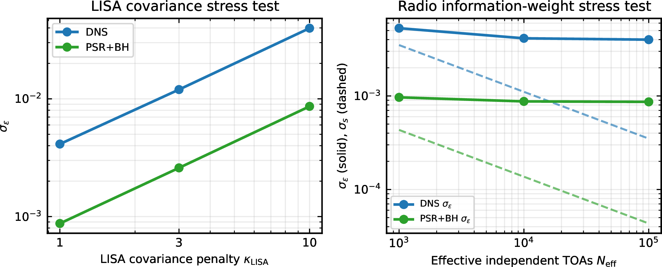
The useful question is therefore not whether the dense grid is a realistic observing schedule; it is how large \(N_{\rm eff}\) must be before the radio contribution is below the LISA one. Figure 4 shows the explicit \(N_{\rm eff}\) dependence for \(10^3\)–\(10^5\) effective samples. Correlated noise with a correlation time comparable to an orbital period can be represented, at this level, by a smaller effective \(N_{\rm eff}\); red spin noise and DM variations are partly absorbed by an inflated effective \(\sigma_{\rm TOA}\), but this is not a substitute for a profile-domain timing analysis. Thus the cadence test is conservative but not exhaustive. A real detection paper must replace this effective treatment by a timing likelihood with the actual cadence and frequency-dependent residuals. The conclusion that the useful benchmarks are mainly LISA-limited survives the conservative radio choice, but the DNS case is no longer radio-negligible by orders of magnitude.
6 LISA forecast model↩︎
On the gravitational-wave side we work with an analytic estimate of the inclination precision rather than a full source-specific LISA covariance matrix. The purpose is to keep the role of the polarization geometry explicit and to show how the resulting residual scales with the detector sensitivity. The signal-to-noise ratio is computed with the sky-averaged LISA sensitivity curve of Robson, Cornish, and Liu [27]. In this convention the response factor is already included in the noise curve. We therefore use the intrinsic tensor amplitude \[h_{\rm rss}=\left(A_+^2+A_\times^2\right)^{1/2},\] and compute \[\rho=h_{\rm rss}\left[\frac{T_{\rm obs}}{S_n(f)}\right]^{1/2}\sqrt{F(e)}. \label{eq:snr}\tag{34}\] The baseline values in Table ¿tbl:tab:forecast? include the time-averaged Galactic confusion term in \(S_n(f)\); Fig. 5 varies a simple local foreground factor to illustrate sky dependence. The inclination error is approximated by the Takahashi–Seto polarimetric Fisher expression [28] \[\sigma_\iota^{\rm LISA}=\frac{1}{\rho}\left[\frac{1+6\cos^2\iota+\cos^4\iota}{4\sin^2\iota(1+\cos^2\iota)^2}\right]^{1/2}. \label{eq:ts02}\tag{35}\] This expression is the sky-averaged, high-SNR, long-observation polarimetric scaling obtained by inverting the Takahashi–Seto Fisher matrix for Galactic binaries after annual modulation has supplied independent tensor-polarization information. Appendix 13 gives the short derivation used here and states which correlations are retained only through the prefactor \(\rho\). Equation 35 should therefore be interpreted as a calibrated scaling ansatz for the inclination variance, not as a source-specific LISA covariance matrix. The use of a sky-averaged SNR together with a modulation-based inclination factor is itself an order-unity compression of the real TDI response. The known radio position, orbital period, and phase evolution should reduce the dimensionality of the LISA fit relative to a blind search, but correlations with polarization angle, amplitude or luminosity distance, residual eccentric harmonics, and imperfect foreground subtraction can still broaden the posterior on \(\iota\) [9], [11], [13]. Although \(d_L\) cancels from the ideal ratio in Eq. 3 , it does not necessarily decouple from the marginalized measurement uncertainty because the detector measures linear combinations of amplitude, polarization angle, phase, and inclination. We therefore do not attempt to calibrate Eq. 35 against a full TDI analysis in this paper, and the quoted numerical sensitivities should be read inside the envelope \(1\leq\kappa_{\rm LISA}\leq10\). For the hypothetical PSR+BH case, Eq. 35 is additionally a monochromatic polarimetric approximation applied to a slowly evolving chirping source; any resulting change in amplitude–phase–inclination covariance is part of what \(\kappa_{\rm LISA}\) is meant to cover. The \(\kappa_{\rm LISA}=3\) column in Table ¿tbl:tab:forecast? and Fig. 4 should therefore be read as a practical robustness check rather than as a calibrated TDI posterior.
To keep this limitation visible, we introduce a covariance-inflation parameter \[\sigma_{\iota}^{\rm LISA,eff}=\kappa_{\rm LISA}\sigma_{\iota}^{\rm TS02}, \label{eq:kappa}\tag{36}\] with \(\kappa_{\rm LISA}=1\) corresponding to the baseline analytic estimate and \(\kappa_{\rm LISA}=3,10\) used to bracket order-unity covariance inflation. This does not replace a TDI likelihood, but it makes transparent which results depend linearly on the simplified polarimetric model. A source-specific detector-level validation remains future work [13], [29].
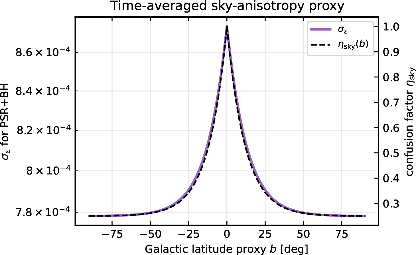
For the Galactic foreground we use the same Robson–Cornish–Liu analytic confusion fit when a sky-averaged comparison is desired [27]. We then introduce a phenomenological local factor \(\eta_{\rm sky}\) such that \[S_n^{\rm eff}(f,\hat{n})=S_n^{\rm inst}(f)+\eta_{\rm sky}(\hat{n})S_n^{\rm conf}(f). \label{eq:conf}\tag{37}\] The factor \(\eta_{\rm sky}\) is not a new LISA foreground model; it is a time-averaged isotropic-equivalent stress parameter that asks how the cross-check changes when the source lies in a cleaner or dirtier sky direction. It does not model the annual modulation of the antenna response or global foreground subtraction. We use \(\eta_{\rm sky}=1\) for the sky-averaged foreground and \(\eta_{\rm sky}=0.5\) as a representative off-plane value. Section 8.2 gives a simple latitude proxy to show the dependence explicitly.
7 Fiducial systems and numerical results↩︎
We consider four representative binaries: a double neutron star (DNS), a pulsar–white-dwarf binary (PSR+WD), an idealized pulsar–black-hole binary (PSR+BH), and a double-pulsar-like longer-period system. These are benchmarks rather than a population model. The PSR+BH row is included as a high-mass-companion scaling case and is explicitly conditional on the discovery of such a system. The PSR+WD and double-pulsar-like rows are useful negative controls: they can be excellent radio systems while remaining poor LISA sources for the adopted periods.
| Class | \(m_p/M_\odot\) | \(m_c/M_\odot\) | \(P_b\) [s] | \(f_{\rm GW}\) [mHz] | \(d\) [kpc] | Role in the forecast |
|---|---|---|---|---|---|---|
| DNS | 1.40 | 1.35 | 900 | 2.222 | 5 | known/future DNS-like; favorable short period |
| PSR+WD | 1.60 | 0.30 | 30600 | 0.065 | 5 | excellent timing but poor LISA source |
| PSR+BH | 1.40 | 10.00 | 900 | 2.222 | 5 | hypothetical; high-SNR chirping case |
| double-pulsar-like | 1.34 | 1.25 | 8640 | 0.231 | 5 | known-like period; weak LISA source |
| Class | \(\rho_{\rm LISA}\) | \(\sigma_\iota^{\rm LISA}\) [deg] | \(\sigma_s^{\rm Shapiro}\) | \(\sigma_\varepsilon\) | \(\sigma_\varepsilon(\kappa_{\rm LISA}=3)\) | \(\sigma_\iota^{\rm joint}\) [deg] |
|---|---|---|---|---|---|---|
| DNS | 72.1 | 0.54 | \(1.11\times10^{-3}\) | \(4.13\times10^{-3}\) | \(1.20\times10^{-2}\) | \(0.144\) |
| PSR+WD | \(<1\) | – | \(6.21\times10^{-3}\) | undetectable | undetectable | – |
| PSR+BH | 332.4 | 0.117 | \(1.37\times10^{-4}\) | \(8.74\times10^{-4}\) | \(2.59\times10^{-3}\) | \(1.83\times10^{-2}\) |
| double-pulsar-like | \(<1\) | – | \(1.43\times10^{-3}\) | undetectable | undetectable | – |
| Class | 7p main | \(7p+\gamma_E\) | 5p reference | 7p loose priors | 7p fixed-\(\omega\) free |
|---|---|---|---|---|---|
| DNS | \(1.11\times10^{-3}\) | \(1.11\times10^{-3}\) | \(1.10\times10^{-3}\) | \(1.11\times10^{-3}\) | \(1.39\times10^{-3}\) |
| PSR+BH | \(1.37\times10^{-4}\) | \(1.37\times10^{-4}\) | \(1.36\times10^{-4}\) | \(1.37\times10^{-4}\) | \(1.88\times10^{-4}\) |
The basic scaling is easy to understand. At fixed inclination and observation time, whenever the radio error is subdominant, \[\sigma_\varepsilon\simeq |\cos\iota|\,\kappa_{\rm LISA}\sigma_\iota^{\rm TS02} \propto \kappa_{\rm LISA}\frac{d\,S_n^{1/2}(2/P_b)}{\mathcal{M}^{5/3}P_b^{-2/3}}. \label{eq:scaling}\tag{38}\] Shorter periods help until the source enters a noisier part of the LISA band or evolves enough that a chirping template is required. Larger companion masses help both the GW amplitude and the Shapiro range. This explains why the hypothetical PSR+BH benchmark performs best, why a short-period DNS remains useful, and why the PSR+WD and double-pulsar-like examples are not useful for the cross-check despite radio timing precision.
Tables ¿tbl:tab:benchmarks? and ¿tbl:tab:forecast? separate the source assumptions from the forecast outputs. The baseline numbers use \(N_{\rm eff}=10^4\), \(\sigma_{\rm TOA}=1\,\mu{\rm s}\), the seven-parameter timing block, and \(\kappa_{\rm LISA}=1\), while the additional \(\kappa_{\rm LISA}=3\) column shows how the result changes when the LISA covariance is inflated by an order-unity factor. For the benchmarks considered here, the useful systems are still mainly LISA-limited, so the residual sensitivity scales almost linearly with \(\kappa_{\rm LISA}\). The quoted \(10^{-3}\)-level values should therefore be read as analytic polarimetric estimates rather than as final detector posteriors. The PSR+BH row is retained as a scaling benchmark rather than a source-count prediction. At the fiducial period its GR inspiral time is about \(4\times10^4\) yr, long on observing times but short enough that the source would be a rare high-SNR system if discovered. The PSR+WD and double-pulsar-like rows make the opposite point: excellent radio timing does not by itself guarantee a useful cross-messenger comparison if LISA polarimetry is uninformative. In the useful regime the comparison is therefore operationally asymmetric: the Shapiro measurement supplies a sharp near-zone reference, and the practical question is whether LISA’s radiative inclination agrees with it. For context, the double pulsar already reaches Shapiro-shape precision at the few \(10^{-5}\) level in long timing solutions [4]; the few-\(10^{-3}\) floor in the DNS forecast is therefore set mainly by LISA rather than by the intrinsic usefulness of Shapiro timing.
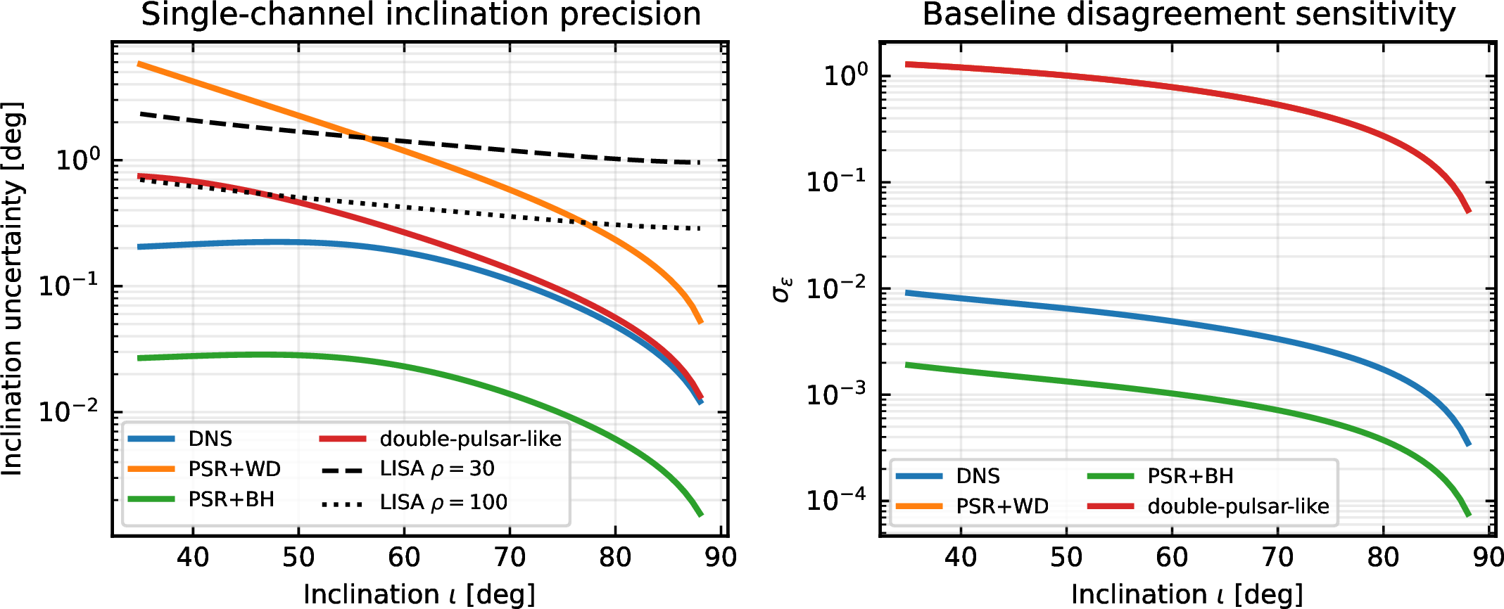
Figure 1 shows the inclination dependence. The face-on region is poor for LISA polarimetry because the polarization ratio changes only weakly with inclination. In the analytic model the residual sensitivity improves toward edge-on because the factor \(|\cos\iota|\,g(\iota)\) decreases and the Shapiro feature sharpens. We therefore no longer identify a formal optimum at \(60^\circ\)–\(80^\circ\); that range is simply a conservative region where the compressed Fisher curves are smooth and less exposed to edge-on response systematics that are not calibrated here.
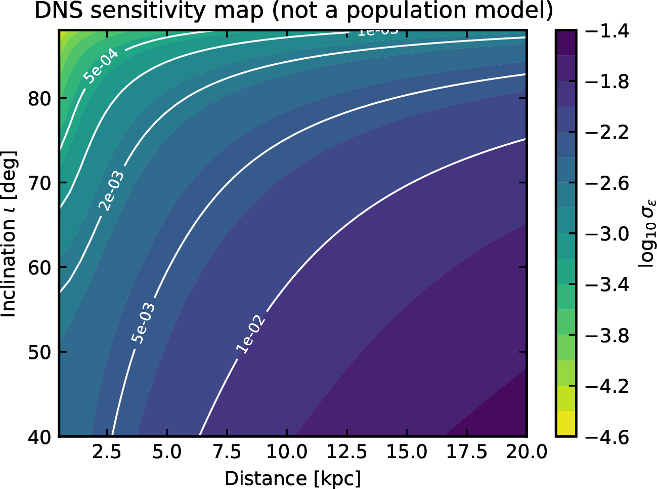
Figure 2 maps a fiducial DNS. The high-precision region tracks LISA SNR and inclination geometry. For Galactic DNS systems within a few kpc and favorable inclination, a baseline sensitivity of a few \(10^{-3}\) is plausible. This is weaker than the best theory-specific orbital-damping bounds, but it is a direct radiative-versus-near-zone consistency test.
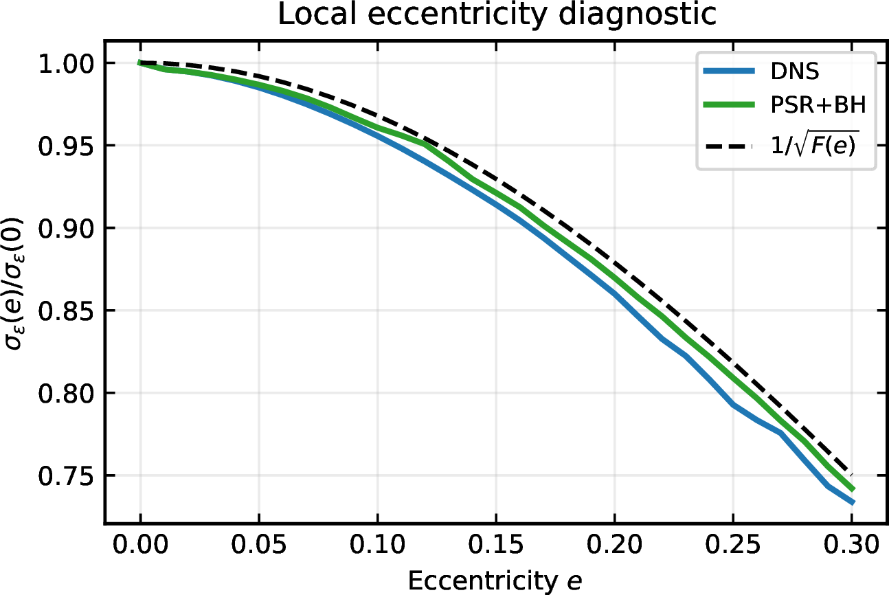
Figure 3 shows a local eccentricity diagnostic, not a population or full eccentric-waveform forecast. The trend should not be overinterpreted. It demonstrates that small eccentricities do not destabilize the timing Fisher calculation and that the leading flat-noise Peters–Mathews SNR effect is mild. A full eccentric-harmonic LISA polarimetry analysis and a timing model with \(\omega(t)\) are required before making precision claims at larger \(e\).
8 Realism analysis and systematics↩︎
8.1 LISA covariance and radio information-weight tests↩︎
The two most important forecast limitations are the simplified LISA inclination estimator and the effective radio cadence model. Rather than claiming a full TDI recovery, we present a transparent analytic baseline and an explicit covariance-penalty scan. We stress-test both in Fig. 4. The left panel varies the LISA covariance factor \(\kappa_{\rm LISA}\) in Eq. 36 . For useful systems, \(\sigma_\varepsilon\) scales almost linearly with this factor because the radiative inclination error dominates. The right panel varies \(N_{\rm eff}=10^3,10^4,10^5\) and also shows the corresponding Shapiro-only error. The radio error follows the expected \(N_{\rm eff}^{-1/2}\) behavior, while \(\sigma_\varepsilon\) is nearly flat once the Shapiro shape is measured accurately enough.
This figure is the main discipline added by the stress-tested forecast. The correct conclusion is not that timing noise never matters. Timing quality is essential for detecting and modeling the Shapiro delay in the first place. The narrower statement is that, conditional on a sufficiently precise Shapiro measurement, further improvements to the radio channel do little for the disagreement statistic until LISA polarimetry is improved.
8.2 Galactic confusion and sky anisotropy↩︎
The unresolved Galactic white-dwarf foreground is anisotropic, concentrated toward the Galactic plane and bulge [29], [30]. A binary pulsar is not a blind LISA source: its sky position, orbital period, and often long-term ephemeris are known from radio observations. This helps reduce the LISA parameter volume and makes the relevant foreground the local time-averaged confusion level along the pulsar direction, not the all-sky average.
To avoid overclaiming, we do not build a synthetic Galaxy or a LISA global foreground fit. We parameterize the local foreground by Eq. 37 . For visualization only, Fig. 5 uses a disk-like proxy \[\eta_{\rm sky}(b)=\eta_{\rm floor}+(1-\eta_{\rm floor})\exp(-|b|/b_0), \label{eq:eta}\tag{39}\] with \(\eta_{\rm floor}=0.25\) and \(b_0=12^\circ\). This \(\eta_{\rm sky}\) is a time-averaged isotropic-equivalent foreground multiplier. It does not model the annual modulation of the LISA antenna pattern or global subtraction residuals. The conclusion is therefore deliberately modest: sky position changes the local confusion penalty at order unity in \(\sigma_\varepsilon\), and a real analysis must replace Eq. 39 by a foreground posterior.
8.3 Chirping of the compact benchmarks↩︎
The quasi-monochromatic approximation is not equally good for all benchmarks. At leading GR order, \[\dot{f}=\frac{96}{5}\pi^{8/3}\left(\frac{G\mathcal{M}}{c^3}\right)^{5/3}f^{11/3}. \label{eq:fdot}\tag{40}\] For the adopted PSR+BH benchmark, \(f=2/P_b=2.22\,{\rm mHz}\) and \(\dot{f}\simeq6.7\times10^{-16}\,{\rm Hz\,s^{-1}}\), so the source drifts by about \(8.5\times10^{-8}\,{\rm Hz}\) in four years, or roughly ten Fourier bins. It must therefore be treated as a high-SNR chirping compact binary rather than as a stationary monochromatic source. The DNS benchmark with the same nominal period drifts by about two bins in this setup; longer-period DNS examples are safer. These numbers do not invalidate the polarimetric scaling, but they mean that the PSR+BH headline value is a baseline chirping-source scaling, not a final stationary-source TDI forecast.
8.4 Periastron advance, orbital-plane precession, and common epoch↩︎
Periastron advance changes \(\omega(t)\) and must be part of the timing ephemeris for eccentric compact systems. At 1PN order, \[\dot{\omega}=\frac{3n}{1-e^2}\left(\frac{GMn}{c^3}\right)^{2/3}, \qquad n=2\pi/P_b . \label{eq:periastron}\tag{41}\] For the fiducial DNS this is several radians per year, and for the PSR+BH benchmark it is tens of radians per year. This is not an optional small correction; it is part of the global timing solution that defines \(\omega(t)\).
The more dangerous effect for the residual itself is a change in the line-of-sight inclination. Spin-orbit precession of a misaligned black-hole companion gives the approximate Lense–Thirring rate \[\Omega_{\rm LT}\simeq \frac{2GJ}{c^2a^3(1-e^2)^{3/2}},\qquad J=\chi\frac{Gm_{\rm BH}^2}{c}, \label{eq:lt}\tag{42}\] which evaluates to \(\Omega_{\rm LT}\simeq0.14\chi\,{\rm rad\,yr^{-1}}\) for the PSR+BH benchmark. This is far larger than the statistical \(\sigma_\varepsilon\) if it is not modeled. The observable must therefore be evaluated at a shared epoch, Eq. 8 , or with a shared orientation model.
A minimal Fisher estimate shows why this requirement is manageable but not negligible. Suppose the data constrain a locally linear orientation variable \(s(t)=s_0+\dot{s}(t-t_{\rm mid})\) over a span \(T\). Uniform information in time gives uncorrelated Fisher errors on \(s_0\) and \(\dot{s}\) at the midpoint, and the variance propagated to an epoch offset \(\Delta t\) is \[\sigma_s^2(\Delta t)=\sigma_s^2(0)\left[1+12\left(\frac{\Delta t}{T}\right)^2\right]. \label{eq:sdot95inflation}\tag{43}\] Thus the common-epoch residual at the middle of the LISA interval is not inflated by fitting a linear orientation drift, while a radio reference epoch one year away from the midpoint of a four-year LISA observation gives an inflation factor \(1.32\), and an endpoint comparison gives a factor \(2\). This is a linearized co-fit estimate. In the strongly misaligned, high-spin PSR+BH corner, where \(\Omega_{\rm LT}T\) can approach several tenths of a radian, curvature in \(s(t)\) makes Eq. 43 a lower-order local estimate rather than a worst-case bound. A full PSR+BH analysis should fit the spin-orbit geometry directly; the precession rate itself would then become a second consistency observable related to frame dragging and the companion spin quadrupole [31], [32].
9 Validation of the Fisher implementation↩︎
Several numerical checks were performed because small sign errors in timing derivatives can change inferred correlations. First, the analytic circular identity in Eq. 33 was compared against direct quadrature of \((\partial_s\Delta_S)^2\) over orbital phase. Agreement is at machine precision except very close to edge-on configurations, where the integrand develops a sharp conjunction feature and direct quadrature requires tighter tolerances. Second, the derivative \(\partial\Delta/\partial u\) in Eq. 24 was checked against finite differences of Eq. 17 . The sign shown in Eq. 24 is the one that agrees with the finite-difference derivative.
Third, the quadrature grid and statistical weight were varied independently. The production calculation uses a dense grid only to evaluate the phase average and scales the matrix by \(N_{\rm eff}\). Increasing the quadrature grid at fixed \(N_{\rm eff}\) changes \(\sigma_s\) by less than a percent once the sharp conjunction feature is resolved, while changing \(N_{\rm eff}\) gives the expected \(N_{\rm eff}^{-1/2}\) scaling of the radio-only uncertainty. This verifies that the dense grid is not being used as hidden statistical weight.
Fourth, the seven-parameter Fisher matrix was compared with five-parameter and enlarged diagnostic matrices. Without external timing information, the enlarged matrix can be ill-conditioned because several derivatives share similar orbital harmonics. This is a physical warning rather than a numerical nuisance: eccentricity and periastron geometry must be fitted in a global timing solution or constrained by priors. The main calculation therefore uses the prior-augmented vector \((s,r,x,P_b,T_0,e,\omega)\) with the modest priors in Eq. 18 . Relaxing these to deliberately loose priors, \(\sigma_e=10^{-2}\) and \(\sigma_\omega=10^{-1}\,{\rm rad}\), leaves the evolving-\(\omega(t)\) local diagnostic nearly unchanged. If the secular periastron information is artificially removed by holding \(\omega\) fixed and fitting unconstrained \((e,\omega)\), the same matrix inflates \(\sigma_s\) by about \(25\)–\(40\%\) for the useful benchmarks. Including a freely fitted \(\gamma_E\sin u\) term changes the Shapiro-only \(\sigma_s\) by less than the quoted precision, as shown in Table ¿tbl:tab:timing95robust?.
Finally, the LISA part was checked against the expected \(1/\rho\) and \(\kappa_{\rm LISA}\) scalings. When distance is varied at fixed frequency and inclination, \(\sigma_\varepsilon\) follows Eq. 38 until the Fisher estimate reaches the imposed physical inclination cap. When \(\kappa_{\rm LISA}\) is varied, useful-system residuals scale almost linearly, demonstrating that the headline sensitivities should be read as baseline polarimetric Fisher values rather than as final TDI posterior widths.
10 Phenomenological interpretation and theory-specific requirements↩︎
The robust quantity in this paper is the residual \(\varepsilon\) and its uncertainty. Mapping \(\varepsilon\) into a theory parameter is necessarily model dependent. In scalar-tensor gravity, for example, the same scalar charges that affect orbital damping can also modify the radiative polarizations and the near-zone lapse, but the relation depends on the neutron-star equation of state, the scalarization branch, the companion type, and the detector response [3], [17], [18]. In vector-tensor, additional-polarization, or Lorentz-violating theories the mapping is different. For pure GW propagation or modified-dispersion effects, \(\varepsilon\) may not respond at all if the polarization amplitude ratio and the Shapiro shape remain unchanged [33].
For this reason we do not present a headline exclusion contour. Such a contour would be less robust than the geometric forecast itself. The correct way to use the present calculation is straightforward: once a theory-specific waveform and a corresponding near-zone timing model are in hand, one computes \(s_{\rm GW}\) and \(s_{\rm Shapiro}\) consistently and compares them through Eq. 8 . The value of the construction lies in the fact that the two sides of the comparison are independently measurable and arise from physically distinct sectors of the problem.
11 Data-analysis roadmap↩︎
The calculation presented here is analytic by construction, but the observable is naturally suited to a full Bayesian analysis. The radio likelihood would be the usual timing likelihood with a binary model containing Shapiro, Roemer, Einstein, and post-Keplerian terms. The LISA likelihood would use the known radio sky position and an orbital-frequency prior, while allowing independent amplitude, polarization, phase, and inclination parameters. A minimal consistency analysis would sample \[\{\boldsymbol{\lambda}_{\rm common},s_{\rm Shapiro},s_{\rm GW},\boldsymbol{\lambda}_{\rm radio},\boldsymbol{\lambda}_{\rm LISA}\},\] where \(\boldsymbol{\lambda}_{\rm common}\) contains quantities such as sky position and orbital frequency, while \(\boldsymbol{\lambda}_{\rm radio}\) and \(\boldsymbol{\lambda}_{\rm LISA}\) contain nuisance parameters specific to each messenger. The posterior on \(\varepsilon\) would then be obtained directly from posterior samples rather than from the Fisher approximation. Because \(s=\sin\iota\) is reflection-invariant, the ordinary \(\iota\leftrightarrow\pi-\iota\) ambiguity should be carried through the LISA sampling but normally collapses to the same \(s_{\rm GW}\) posterior. Branch-specific bookkeeping becomes important only when response-dependent non-tensor leakage or sign conventions in the orbital ephemeris are being interpreted.
Such an analysis should include three practical ingredients. First, the LISA model should use time-delay interferometry channels and the time-dependent antenna pattern. The radio position fixes the sky location, but the annual modulation and polarization angle still determine how well the two tensor amplitudes can be separated. Second, the Galactic foreground should be included as either a fitted stochastic component or a realization-dependent residual from a global foreground subtraction. A single scalar factor \(\eta_{\rm sky}\) is sufficient for the comparisons carried out in this paper, but not for data analysis. Third, the timing model should include realistic cadence, pulse-profile evolution, DM variations, clock and ephemeris terms, and where needed a profile-domain treatment rather than idealized Gaussian TOAs.
The Fisher calculation remains useful because it identifies which pieces of such a full analysis matter. The timing channel is not the limiting error source once the Shapiro shape is detected. Therefore, improving radio timing beyond the point where \(\sigma_s\ll |\cos\iota|\sigma_\iota^{\rm LISA}\) gives little gain for the null residual, although it improves the common-inclination estimate. Conversely, improvements in LISA polarimetry, foreground subtraction, and source localization directly improve \(\sigma_\varepsilon\). This prioritization is the main practical result for planning a future LISA–SKA analysis.
The first realistic application need not be a broad population study. A more useful next step would be an injection campaign for a small set of systems spanning the regimes in Tables ¿tbl:tab:benchmarks? and ¿tbl:tab:forecast?: one nearby DNS, one unfavorable low-frequency binary, and one high-mass companion case. For each injection one can compare the Fisher estimate of \(\sigma_\varepsilon\) with the posterior width recovered from the full LISA–radio likelihood. Agreement within a factor of order unity would validate the analytic estimate; large discrepancies would identify the detector-response correlations or timing systematics that matter most. Either outcome would be informative, because the geometric definition of \(\varepsilon\) itself is unchanged.
12 Conclusions↩︎
We have proposed a geometric multimessenger null test that compares the inclination inferred from the LISA tensor polarization ratio with the inclination inferred from the Shapiro-delay shape in the same compact binary pulsar, referenced to a common epoch. The observable is the residual \(\varepsilon(t_0)=s_{\rm Shapiro}(t_0)-s_{\rm GW}(t_0)\). In general relativity it vanishes. A nonzero value would indicate either an unmodeled systematic or a mismatch between the near-zone and radiative descriptions of the binary geometry.
Using representative Galactic systems, we estimated the attainable precision on this residual with timing and GW Fisher calculations that keep the main sources of covariance visible. The timing side includes the Roemer–Shapiro degeneracy, explicit Damour–Taylor derivatives, an Einstein-delay robustness check, and a clear separation between dense phase quadrature and the effective information weight carried by the radio data. The gravitational-wave side uses the Takahashi–Seto inclination scaling together with an explicit covariance-inflation factor to bracket the missing source-specific LISA response. In this conservative baseline, a favorable DNS reaches \(\sigma_\varepsilon\simeq4\times10^{-3}\) and provides the robust astrophysical benchmark. A hypothetical PSR+BH system can reach \(\sigma_\varepsilon\simeq9\times10^{-4}\), but should be read as a high-SNR scaling case that would require discovery of such a system and a chirping LISA template.
The main practical conclusion is simple. Once a compact binary pulsar has a reliable Shapiro measurement, the uncertainty in the null residual is set primarily by gravitational-wave polarimetry rather than by ever denser radio timing. Improvements in LISA polarimetry, foreground subtraction, and source localization therefore matter most for this comparison. The next step is a joint Bayesian analysis using TDI injections with known radio ephemerides, realistic foreground residuals, and a timing likelihood with cadence and secular orientation effects. The present calculation provides the analytic target for that future work.
I thank colleagues in the gravitational-wave group for discussions that shaped the framing of this work. Mainly I would like to thank Apratim Ganguly and Sanjit Mitra.
13 Relation of Eq. 35 to the Takahashi–Seto Fisher scaling↩︎
This appendix summarizes the origin and limitations of Eq. 35 . The leading tensor waveform may be written as two orthogonal quadratures with amplitudes proportional to \[A_+=A_0(1+u^2),\qquad A_\times=2A_0u, \label{eq:app95amp}\tag{44}\] where \(u=\cos\iota\). In a long LISA observation, annual orbital motion modulates the response and supplies information that partially separates the two tensor amplitudes and the polarization angle. Takahashi and Seto computed the corresponding Fisher matrix for Galactic binaries and expressed the inclination uncertainty as a geometric factor times \(1/\rho\) [28]. In the simplified sky-averaged limit used in the present forecast, the amplitude and phase information enter only through the total SNR, leaving \[\sigma_\iota = \rho^{-1}\,g(\iota), \qquad g^2(\iota)=\frac{1+6u^2+u^4}{4(1-u^2)(1+u^2)^2}, \label{eq:app95ts02}\tag{45}\] which is Eq. 35 . The numerator encodes the residual amplitude–polarization covariance of the tensor quadratures; the factor \(1-u^2=\sin^2\iota\) gives the familiar degradation near face-on orientation.
This expression is therefore not a statement that distance, polarization angle, and initial phase are known perfectly. Rather, it is a compact analytic representation of a more complete LISA Fisher calculation, using the SNR and inclination as the quantities most directly relevant for the cross-messenger residual. A full TDI likelihood with source-specific sky position, annual modulation, eccentric harmonics, and a foreground model can change the prefactor by factors of order unity or more. This is why we introduce \(\kappa_{\rm LISA}\) in Eq. 36 and quote the interval \(1\leq\kappa_{\rm LISA}\leq10\) as the present forecast envelope.
14 Derivation of the circular Shapiro identity↩︎
At \(e=0\), the Shapiro delay is \[\Delta_S=-2r\ln(1-s\sin\phi),\] so \[\partial_s\Delta_S=\frac{2r\sin\phi}{1-s\sin\phi}.\] The orbit average is \[I_s=4r^2\left\langle\frac{\sin^2\phi}{(1-s\sin\phi)^2}\right\rangle, \qquad \langle X\rangle\equiv\frac{1}{2\pi}\int_0^{2\pi}X(\phi)\,\mathrm{d}\phi,\] valid for \(|s|<1\), with the edge-on limit approached by continuity. Using \[\frac{\sin^2\phi}{(1-s\sin\phi)^2}=\frac{1}{s^2}\left[1-\frac{2}{1-s\sin\phi}+\frac{1}{(1-s\sin\phi)^2}\right]\] and \[\begin{align} \left\langle\frac{1}{1-s\sin\phi}\right\rangle &= \frac{1}{\sqrt{1-s^2}},\nonumber\\ \left\langle\frac{1}{(1-s\sin\phi)^2}\right\rangle &= \frac{1}{(1-s^2)^{3/2}}, \end{align}\] one obtains Eq. 33 . The small-\(s\) expansion verifies the finite face-on limit. The often-quoted but incorrect form \(4r^2s^2/(1-s^2)^{3/2}\) results from keeping only the final squared-denominator integral and dropping the two lower-order terms generated by the algebraic identity above; it therefore fails the \(s\to0\) check.
15 Seven-parameter timing derivatives↩︎
For completeness, we give the additional derivatives needed when \(e\) and \(\omega\) are included in the Fisher vector. At fixed \(u\), \[\begin{align} q_\omega &\equiv \frac{\partial q}{\partial\omega}=\cos\omega(\cos u-e)-\sqrt{1-e^2}\sin\omega\sin u,\nonumber\\ q_e\big|_u &\equiv \left.\frac{\partial q}{\partial e}\right|_u=-\sin\omega-\frac{e}{\sqrt{1-e^2}}\cos\omega\sin u. \end{align}\] Kepler’s equation gives \[\frac{\partial u}{\partial e}=\frac{\sin u}{1-e\cos u}\] at fixed \(M\). The full derivatives are then \[\begin{align} \frac{\partial\Delta}{\partial\omega} &= xq_\omega+\frac{2rsq_\omega}{A},\nonumber\\ \frac{\partial\Delta}{\partial e} &= xq_e\big|_u+\frac{2r}{A}\left(\cos u+s q_e\big|_u\right)+\frac{\partial\Delta}{\partial u}\frac{\sin u}{1-e\cos u}. \end{align}\] The accompanying code uses this seven-parameter Fisher matrix for the fiducial timing entries, with Gaussian priors on \(e\) and \(\omega\) standing in for the information supplied by the global timing solution. The five-parameter matrix is retained only as a diagnostic comparison.