Painlevé and collisionless shock in the defocusing NLS equation with step-like initial data in the transition regions
June 25, 2026
Abstract
We consider the Cauchy problem for the defocusing nonlinear Schrödinger (NLS) equation with step-like initial data \[\begin{align}
{2} &\mathrm{i}u_t+u_{xx}-2|u|^2u=0, \quad x\in\mathbb{R},\quad t> 0, \nonumber\\
&u(0, x) \sim
\alpha\mathrm{e}^{2\mathrm{i}\beta x}, \;\;x\to -\infty;\;\;
u(0, x) \sim 0, \;\; x\to +\infty, \nonumber
\end{align}\] where \(\alpha>0\) and \(\beta\in\mathbb{R}\) are two parameters. Using the nonlinear steepest descent method, we derive the long-time asymptotic expansion of the
solution to the Cauchy problem in three distinct transition regions. In the first two transition regions, the leading-order asymptotics are characterized by Painlevé -type formula, while in the third one is a collisionless shock region, the leading-order
asymptotics is describedin terms of Riemann theta functions. Our analysis is based on the Riemann-Hilbert formulation associated with the Cauchy problem of the defocusing NLS equation.
Key words: Defocusing NLS equation, Riemann-Hilbert problem, nonlinear steepest descent method, long-time asymptotics, Painlevé , collisionless shock wave.
MSC 2020: 35Q51; 35Q15; 35C20; 35P25; 34M55.
1 Introduction↩︎
The defocusing nonlinear Schrödinger (NLS) equation \[\begin{align} {2} &\mathrm{i}u_t+u_{xx}-2|u|^2u=0, &\qquad&x\in\mathbb{R},\quad t> 0 \label{equ:nls} \end{align}\tag{1}\] is one of the most important integrable equations in mathematical physics. Since 1950s [1], when its connection with the theory of superconductivity was discovered, the NLS equation is widely viewed as an important model in describing a variety of physical phenomena, which include water waves [2], surface gravity waves [3], nonlinear optics [4], [5], plasmas [6] and Bose-Einstein condensates [7].
In this paper, we investigate long-time asymptotics in three transition regions to the solution of the Cauchy problem for the NLS equation 1 with a step-like initial data \[\begin{align} {2} &u(x,0)=u_0(x)\to \begin{cases} \alpha\mathrm{e}^{2\mathrm{i}\beta x}, &x\to -\infty,\\ 0, &x\to +\infty, \end{cases} \label{Initial32data} \end{align}\tag{2}\] where \(\alpha>0\) and \(\beta\in\mathbb{R}\) are two parameters. Further we assume that the solution \(u(x,t)\) vanishes as \(x\to+\infty\) and approaches to a plane wave as \(x \to - \infty\), i.e., \[\label{boundaryconditions} u(x,t)\to \begin{cases} \alpha\mathrm{e}^{2\mathrm{i}\beta x+\mathrm{i}\omega t}, & x\to -\infty, \\ 0, & x\to +\infty, \end{cases}\tag{3}\] where the constant \(\omega:=-4\beta^2-2\alpha^2<0\) in 3 is determined by the requirement that \(\alpha\mathrm{e}^{2\mathrm{i}\beta x+\mathrm{i}\omega t}\) should be a solution to 1 . The phase invariance of 1 implies that there is no loss of generality in assuming that \(\alpha\) is positive. To ensure compatibility of the boundary conditions 3 with the evolution 1 –2 .
The study of long-time asymptotics for Cauchy problems of nonlinear integrable systems with step-like initial data has a long history and can be traced back to the pioneering work [8] of Gurevich and Pitaevskii on the Korteweg-de Vries (KdV) equation. Working within the framework of Whitham modulation theory [9], they predicted the emergence of highly oscillatory structures, now referred to as dispersive shock waves in the long-time dynamics. The rigorous mathematical justification of this phenomenon was subsequently done by Khruslov [10] via the inverse scattering transform in terms of the Marchenko integral equations and the so-called asymptotic soliton. Rigorous asymptotic analysis of step-like Cauchy problems for integrable partial differential equations (PDEs) began with the papers [11], [12]. Since then, the long-time asymptotics of integrable PDEs with step-like initial data have been extensively studied: for the KdV equation [13], [14]; for the focusing nonlinear Schrödinger equation (NLS) [15]–[17]; for the focusing mKdV equation [18]–[22]; as well as for some nonlocal integrable PDEs [23]–[26].
Establishing transition asymptotics for integrable nonlinear PDEs is usually a challenging task, which typically involve the nonlinear special functions – Painlevé transcendents and exhibit some universal features. For instance, one encounters the Painlevé II transcendents and its higher order analogues in [27]–[34], the Painlevé I transcendents and its higher order analogues in [35], [36], and a model RH problem associated with the Painlevé IV equation in [37]. In the present work, we shows that the analysis in the first two transition regions involves RH problems relevant to the Painlevé XXXIV transcendents, which is different from the classical local parametrices used in the analysis in the other regions [38]. To be precise, the Painlevé equation, which reads as \[u''(s)=4u(s)^2+2su(s)+\frac{u'(s)^2-(2b)^2}{2u(s)},\] depends on a parameter \(b\). This equation can be obtained from the well-known Painlevé equation \[q''(s)=sq(s)+2q^3-\nu,\quad \nu=2b+\frac{1}{2},\] and its Hamiltonian [39], [40]. The Painlevé transcendents play an important role in asymptotic studies of critical behaviors arsing from integrable differential equations [41], [42], random unitary ensembles [39] and orthogonal polynomials [43]. While in the third transition region, we discover a new phenomenon which is called the collisionless shock region. This phenomenon, first discovered by Gurevich and Pitaevski (see [44]) in their analysis of a shock solution for the KdV equation with shock initial data, is also observed in the long-time asymptotics for the KdV equation with Schwarz-type initial data [45], [46], for the Camassa-Holm (CH) equation on the half-line [47], and for the modified Camassa-Holm (mCH) equation with finite-density initial data [34].
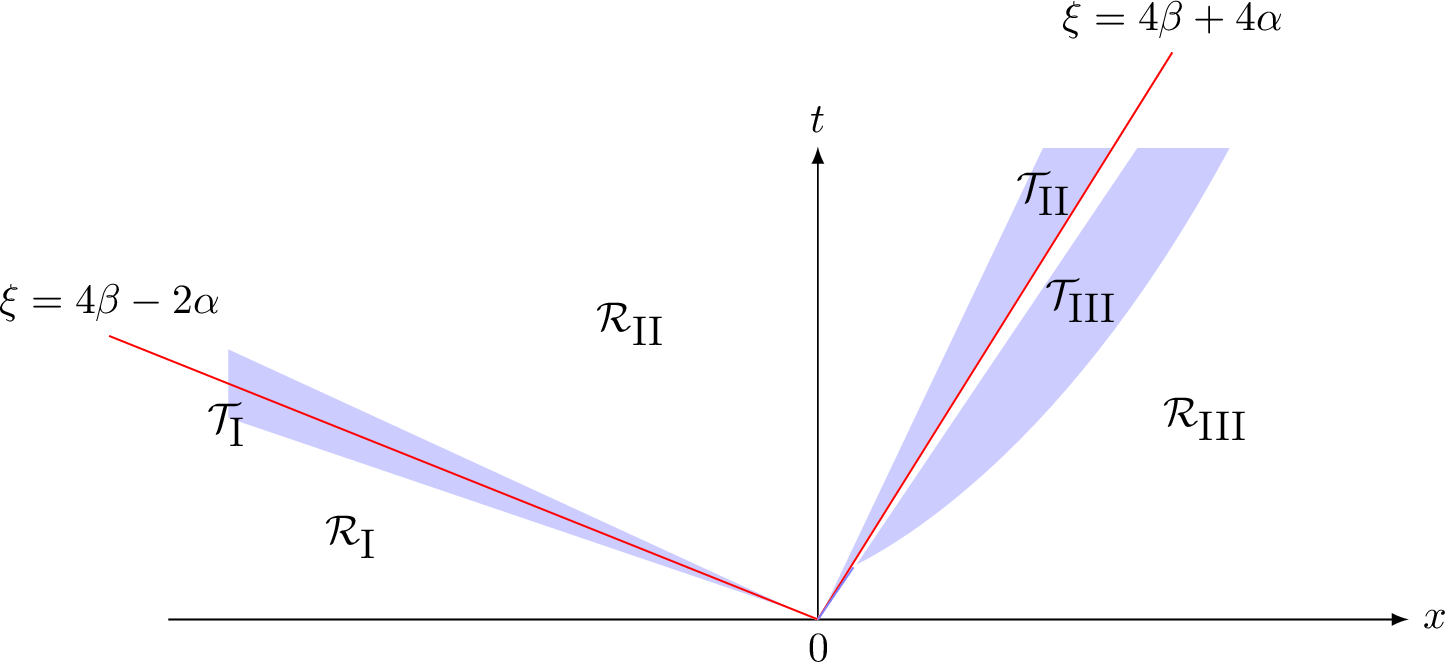
In recent papers [48], [49], Fromm, Lenells and Quirchmayr proved that there exists a global solution of the defocusing NLS equation in 1 –2 under the asymptotically step-like boundary conditions 3 and obtain its long-time asymptotics to equation 1 in these different regions. More precisely, these regions are defined as follows (see Figure 1):
Left-most region \(\mathcal{R}_{\mathrm{\uppercase{\romannumeral1}}}\):= \(\left\{(x,t): \xi<4\beta-2\alpha \right\}\),
Middle region \(\mathcal{R}_{\mathrm{\uppercase{\romannumeral1}}}\):= \(\left\{(x,t): 4\beta-2\alpha<\xi<4\beta+4\alpha \right\}\),
Right-most region \(\mathcal{R}_{\mathrm{\uppercase{\romannumeral3}}}\):= \(\left\{(x,t): \xi>4\beta+4\alpha \right\}\),
where \(\xi:=\frac{x}{t}\). To summarize, in \(\mathcal{R}_{\mathrm{\uppercase{\romannumeral1}}}\), the leading term is given by the plane wave \(\alpha\mathrm{e}^{2\mathrm{i}\beta x+\mathrm{i}\omega t}\) multiplied by a slowly varying factor which tends to 1 as \(\xi\to-\infty\) and the sub-leading term is expressed in terms of the parabolic cylinder function [48]; in \(\mathcal{R}_{\mathrm{\uppercase{\romannumeral2}}}\), the leading term is given by a slowly varying factor, while the sub-leading term is derived from the Airy function [48]; in \(\mathcal{R}_{\mathrm{\uppercase{\romannumeral3}}}\), the leading term is of order \(t^{-1/2}\) with a coefficient which vanishes as \(\xi\to+\infty\) [48]. Thus, the remaining problem is to characterize the long-time asymptotic behavior in the regions adjacent to these three regions, namely the transition regions, as illustrated in Figure 1.
1.1 Main results↩︎
Besides the boundary condition 3 , we assume that the initial data \(u_0(x)\) satisfies the following conditions.
Assumption 1.
\(x^m\left(u_0-\alpha\mathrm{e}^{2\mathrm{i}\beta x}\right)|_{\mathbb{R}^-}\in L^1(\mathbb{R}^-)\), \(x^mu_0|_{\mathbb{R}^+}\in L^1(\mathbb{R}^+)\), \(m=0,\cdots,8\).
\(u_0\in\mathcal{C}^4(\mathbb{R})\), \(\partial_x^n u_0\in L^\infty(\mathbb{R})\), \(n=0,\cdots,3\).
We next give the precise definition of the different transition regions in the \((x,t)\)-half plane.
Definition 1. For constants \(\alpha>0\) and \(\beta\in\mathbb{R}\), we define
The first transition region \(\mathcal{T}_{\mathrm{\uppercase{\romannumeral1}}}:=\left\{(x,t): \left|\xi-(4\beta-2\alpha)\right|t^{\frac{2}{3}}<C\right\}\).
The second transition region \(\mathcal{T}_{\mathrm{\uppercase{\romannumeral2}}}:=\left\{(x,t): 0<\left(4\beta+4\alpha-\xi\right)t^{\epsilon}<C,\epsilon<\frac{1}{2}\right\}\).
The third transition region \(\mathcal{T}_{\mathrm{\uppercase{\romannumeral3}}}:=\left\{(x,t): C<\sqrt{\frac{t}{\log t}}\left[\xi-4(\alpha+\beta)\right]<2^{-\frac{3}{4}}\right\}\).
Here \(\xi=x/t\); see Figure 1 for an illustration.
Long-time asymptotics of the solution \(u(x,t)\) in each of the regions given in Definition 1 are main results of the present work.
Theorem 1. Let \(u(x,t)\) be the global solution of the Cauchy problem 1 –2 for the defocusing NLS equation over the real line under Assumption 1, and denote by \(r(k)\) the reflection coefficient. As \(t\rightarrow+\infty\), we have the following asymptotics of \(u(x,t)\) in the following three transition regions.
For \(\xi\in\mathcal{T}_{\mathrm{\uppercase{\romannumeral1}}}\), we have \[\begin{align} \label{asy32formula:TI} u(x,t)=-\mathrm{e}^{2\mathrm{i}\beta x+\mathrm{i}\omega t}D_{\mathrm{\uppercase{\romannumeral1}},\infty}^{-2}(\xi)\left[\alpha+t^{-1/3}f_{\mathrm{\uppercase{\romannumeral1}}}(\xi,s)\right]+\mathcal{O}(t^{2/3-2\epsilon_1}), \end{align}\qquad{(1)}\] where \(\epsilon_1\) is any real number with \(\frac{1}{2}<\epsilon_1<\frac{2}{3}\) and \[\begin{align} & D_{\mathrm{\uppercase{\romannumeral1}},\infty}(\xi)=\exp\left[-\frac{1}{2\pi \mathrm{i}} \left(\int_{-\infty}^{E_1}\frac{\log \left(1-r(z)r^*(z)\right)}{X(z)}\mathop{}\!\mathrm{d}z+\int_{E_1}^{E_2} \frac{\log r(z)}{X_{+}(z)}\mathop{}\!\mathrm{d}z\right)\right],\\ &s=-t^{\frac{2}{3}}\frac{g_{\mathrm{\uppercase{\romannumeral1}}}^{(1)}(E_2)}{\left(\frac{3}{2}\right)^{\frac{1}{3}}\left|g_{\mathrm{\uppercase{\romannumeral1}}}^{(2)}(E_2)\right|^{\frac{1}{3}}},\; f_\mathrm{\uppercase{\romannumeral1}}(\xi,s)=-\frac{\mathrm{i}}{4}\left(\frac{3}{2}\right)^{-\frac{1}{3}}(2\alpha)^{\frac{1}{2}}\left|g_{\mathrm{\uppercase{\romannumeral1}}}^{(2)}(E_2)\right|^{-\frac{1}{3}}s^2 \end{align}\] with \[\begin{align} & g_{\mathrm{\uppercase{\romannumeral1}}}^{(1)}(E_2)=2\alpha(\xi+2\alpha-4\beta),\quad g_{\mathrm{\uppercase{\romannumeral1}}}^{(2)}(E_2)=\frac{\xi+2\alpha-4\beta}{2\sqrt{2\alpha}}+4\alpha. \end{align}\]
For \(\xi\in\mathcal{T}_{\mathrm{\uppercase{\romannumeral2}}}\), we have \[\begin{align} \label{asy32formula:RII} u(x,t)=2\mathrm{i}\mathrm{e}^{2\mathrm{i}tg_{\mathrm{\uppercase{\romannumeral2}},\infty}(\xi)} D_{\mathrm{\uppercase{\romannumeral2}},\infty}^{-2}(\xi)\left[\frac{4\alpha+4\beta-\xi}{6}+t^{-1/3}f_{\mathrm{\uppercase{\romannumeral2}}}(\xi,s)\right]+\mathcal{O}(t^{-1/2}), \end{align}\qquad{(2)}\] where \[\begin{align} &g_{\mathrm{\uppercase{\romannumeral2}},\infty}(\xi)=\frac{\xi^2-4E_1\xi-8E_1^2}{12},\\ &D_{\mathrm{\uppercase{\romannumeral2}},\infty}(\xi)=\exp\left[-\frac{1}{2\pi \mathrm{i}} \left(\int_{-\infty}^{E_1}\frac{\log \left(1-r(p)r^*(p)\right)}{\mathcal{X}(p)}\mathop{}\!\mathrm{d}p+\int_{E_1}^{k_0} \frac{\log r(p)}{\mathcal{X}_{+}(p)}\mathop{}\!\mathrm{d}p\right)\right],\\ &s=-2\left(\frac{9}{2}\right)^{-\frac{1}{3}}t^{\frac{2}{3}}(k_0-E_1)^{\frac{4}{3}},\quad f_{\mathrm{\uppercase{\romannumeral2}}}(\xi,s)=\left(\frac{27}{2}\right)^{-\frac{1}{3}}(4\alpha+4\beta-\xi)^{\frac{1}{3}}a(s). \end{align}\] Here, \(a(s)\) can be calculated by \[a(s)=\int_{-\infty}^s \left( u(p) + \frac{p}{2}\right) \mathop{}\!\mathrm{d}p,\] where \(u(s)\) is the unique solution of the Painlevé equation \[u''(s)=4u(s)^2+2su(s)+\frac{u'(s)^2-\frac{1}{4}}{2u(s)}\] which satisfies \[u(s)=\left\{ \begin{array}{ll} \frac{1}{-4\sqrt{s}}+\mathcal{O} \left( s^{-2} \right) , &\qquad s\to +\infty, \\ -\frac{s}{2}+\mathcal{O} \left( s^{-2} \right) , &\qquad s\to -\infty. \end{array}\right .\]
For \(\xi\in\mathcal{T}_{\mathrm{\uppercase{\romannumeral3}}}\), we have \[\label{asy32formula:RIII} \begin{align} u(x,t)=&\frac{\left[\xi-4(\alpha+\beta)\right] (a-b)}{4}\mathrm{e}^{2\mathrm{i}t\left[g_{\mathrm{\uppercase{\romannumeral3}},\infty}(\xi)-(\alpha+\beta)^2+\frac{\xi}{2}(\alpha+\beta)\right]+\mathrm{i}\phi} \frac{\Theta\left(-\mathcal{A}(\infty)+\frac{E}{4}-\frac{\phi}{\pi}\right) \Theta\left(\mathcal{A}(\infty)+\frac{E}{4}\right)}{ \Theta\left(\mathcal{A}(\infty)+\frac{E}{4}-\frac{\phi}{\pi}\right)\Theta\left(-\mathcal{A}(\infty)+\frac{E}{4}\right)}\\ &+\mathcal{O}(1), \end{align}\qquad{(3)}\] where \(\Theta(s)\) is the Jacobi theta function defined by 95 with the Abel map \(\mathcal{A}(z)\) given in 96 . Moreover, the quantities \(E\) and \(\phi\) are defined in 112 and 98 respectively and the parameters \(a\) and \(b\) are uniquely defined by equations 82 and ?? .
Remark 2. It is worth noting that a small region between the Painlevé region \(\mathcal{T}_{\mathrm{\uppercase{\romannumeral2}}}\) and the collisionless shock region \(\mathcal{T}_{\mathrm{\uppercase{\romannumeral3}}}\) lies outside the scope of the present discussion, and its characterization remains an open question.
1.2 Outline of this paper↩︎
The organization of our paper is as follows. In Section 2, we quickly review some basic results, especially the construction of a basic RH formalism \(M(z)\) associated with the Cauchy problem 1 –2 . For more details, see [48]. In Section 3, we focus on the long-time asymptotic analysis for the defocusing NLS equation in the transition region \(\mathcal{T}_{\mathrm{\uppercase{\romannumeral1}}}\). In Subsections 3.1–3.5, we use nonlinear steepest descent method to deform the RH problem \(M(z)\) into a solvable RH Painlevé XXXIV model given in Appendix 6. Finally, in the last subsection 3.6, we complete the proof of () of Theorem 1. In Section 4, we obtain the Painlevé XXXIV asymptotics for the defocusing NLS equation in the transition region \(\mathcal{T}_{\mathrm{\uppercase{\romannumeral2}}}\) with similar steps to Section 3. In Section 5, we carry out the asymptotic analysis in the third transition region \(\mathcal{T}_{\mathrm{\uppercase{\romannumeral3}}}\), which is a collisionless shock region, the leading-order asymptotics is describedin terms of Riemann theta functions. A key step in this case is to apply the g-function mechanism developed in [46] to arrive at a model RH problem solvable in terms of the Riemann theta function. The o proof of part (III) of Theorem 1 is presented in Subsection 5.7.
1.3 Notations↩︎
Throughout this paper, we adopt the following notations.
As usual, the classical Pauli matrices \(\{\sigma_j\}_{j=1,2,3}\) are defined by \[\sigma_1:=\begin{pmatrix}0 & 1 \\ 1 & 0\end{pmatrix}, \quad \sigma_2:=\begin{pmatrix}0 & -\mathrm{i}\\ \mathrm{i}& 0\end{pmatrix}, \quad \sigma_3:=\begin{pmatrix}1 & 0 \\ 0 & -1\end{pmatrix}.\] For a \(2\times 2\) matrix \(A\), we also define \[\mathrm{e}^{\hat{\sigma}_j}A:=\mathrm{e}^{\sigma_j}A\mathrm{e}^{-\sigma_j}, \quad j=1,2,3.\]
For a complex-valued function \(f(z)\), we use \(f^{*}(z):=\overline{f(\bar{z})}\) for \(z\in\mathbb{C}\) to denote its Schwartz conjugation.
For a region \(U\subseteq \mathbb{C}\), we use \(U^*\) to denote the conjugated region of \(U\). We also set \[\mathbb{C}^{\pm}:=\left\{z \in\mathbb{C}: \pm \text{Im}\;z>0 \right\},\qquad \mathbb{R}^{\pm}:=\left\{z \in\mathbb{R}: \pm z>0 \right\}.\]
For \(1 \leqslant p < \infty\), the \(L^p\)-space is defined as: \[L^p(\mathbb{R}) = \left\{ f: \mathbb{R} \to \mathbb{C} \;\middle| \;f \text{ is measurable and } \|f\|_p < \infty \right\},\] where the \(L^p\)-norm is given by \(\|f\|_p = \left( \int_{\mathbb{R}} |f(x)|^p dx \right)^{1/p}\). For \(p = \infty\), the \(L^\infty\)-space is defined by \[L^\infty(\mathbb{R}) = \left\{ f: \mathbb{R} \to \mathbb{C} \;\middle| \;f \text{ is measurable and } \|f\|_\infty < \infty \right\},\] where the essential supremum norm is given by \(\|f\|_\infty = \inf \left\{ M \geqslant 0 \;| \;|f(x)| \leqslant M \text{ a.e.} \right\}.\) The \(\mathcal{C}^{N}(\Omega)\), \(N=1,2,\dots,\infty\) is defined as the space of \(N\)-times continuously differentiable functions on \(\Omega\).
For any smooth oriented curve \(\Sigma\), the Cauchy operator \(\mathcal{C}\) on \(\Sigma\) is defined by \[\begin{align} \mathcal{C}f(z)=\frac{1}{2\pi \mathrm{i}}\int_{\Sigma}\frac{f(y)}{y-z}\mathop{}\!\mathrm{d}y, \qquad z\in\mathbb{C}\setminus \Sigma. \end{align}\] Given a function \(f \in L^p(\Sigma)\), \(1\leqslant p<\infty\), \[\begin{align} \label{def:opCpm} \mathcal{C}_\pm f(z):=\lim_{\substack{z'\to z\in\Sigma\\ z'\in\pm\text{ side of } \Sigma}}\frac{1}{2\pi \mathrm{i}}\int_{\Sigma}\frac{f(y)}{y-z'}\mathop{}\!\mathrm{d}y \end{align}\tag{4}\] stands for the positive/negative (according to the orientation of \(\Sigma\)) non-tangential boundary value of \(\mathcal{C}f\).
If \(A\) is a matrix, then \((A)_{ij}\) stands for its \((i,j)\)-th entry, and \([A]_j\) represents the \(j\)-th column. We use \(A^{\rm H}\) to denote its conjugate transpose, which means \(A^{\rm H}=\bar A^{\rm T}\).
We use the notation \(a\lesssim b\) (resp.\(a \gtrsim b\)) to indicate that \(a\leqslant Cb\) (resp.\(a\geqslant Cb\)) for some generic positive constant \(C\).
2 Spectral analysis and inverse scattering transform↩︎
In this section, we state some main results on the inverse scattering transform associated with the Cauchy problem 1 –2 . The details can be found in [48].
2.1 Direct scattering transform↩︎
The Lax pair of the defocusing NLS equation 1 is given by \[\begin{align} \label{equ:lax32pair} \left\{ \begin{aligned} &\Phi_x+\mathrm{i}k\sigma_3\Phi=Q\Phi, \\ &\Phi_t+2\mathrm{i}k^2\sigma_3\Phi=V\Phi, \end{aligned} \right. \end{align}\tag{5}\] where \(\Phi=\Phi(k;x,t)\) is a \(2\times 2\) matrix-valued function with the spectral parameter \(k\in\mathbb{C}\). Here, \(Q\) and \(V\) are some matrices associated with the potential function \(u\) defined by \[\begin{align} Q=\begin{pmatrix}0 & u \\ \bar u & 0\end{pmatrix}, \quad V=\begin{pmatrix} -\mathrm{i}|u|^2 & 2ku+\mathrm{i}u_x\\2k\bar u-\mathrm{i}\bar u_x&\mathrm{i}|u|^2 \end{pmatrix}.\label{equ:Q40x44t4144V40x44t41} \end{align}\tag{6}\]
Substituting the plane wave solution \(u =\alpha\mathrm{e}^{2\mathrm{i}\beta x+\mathrm{i}\omega t}\) of 1 into 5 , we obtain the corresponding “background” Lax pair \[\label{laxpair:background} \left\{ \begin{align} &\Phi^b_{l,x}+\mathrm{i}k\sigma_3\Phi^b_l=Q^b_l\Phi^b_l, \\ &\Phi^b_{l,t}+2\mathrm{i}k^2\sigma_3\Phi^b_l=V^b_l\Phi^b_l, \end{align} \right.\tag{7}\] where \[\label{equ:Q95j94b44V95j94b} Q^b_l=\begin{pmatrix}0 & \alpha\mathrm{e}^{2\mathrm{i}\beta x+\mathrm{i}\omega t} \\ \alpha\mathrm{e}^{-2\mathrm{i}\beta x-\mathrm{i}\omega t} & 0\end{pmatrix},\quad V^b_l=\begin{pmatrix} -\mathrm{i}\alpha^2&2\alpha(k-\beta)\mathrm{e}^{2\mathrm{i}\beta x+\mathrm{i}\omega t}\\2\alpha(k-\beta)\mathrm{e}^{-2\mathrm{i}\beta x-\mathrm{i}\omega t}&\mathrm{i}\alpha^2 \end{pmatrix}.\tag{8}\] Let \(E_1=-\beta-\alpha\) and \(E_2=-\beta+\alpha\). The explicit solution to the “background” Lax pair 7 is given by \[\label{equ:Phi95j94p} \Phi_{l}^{b}(k;x,t)=\mathrm{e}^{\mathrm{i}\left(\beta x+\frac{\omega}{2}t\right)\sigma_3}\Delta(k)\mathrm{e}^{-\mathrm{i}(X(k)x+\Omega(k)t)\sigma_3},\tag{9}\] where functions \(X,\Omega:\mathbb{C}\setminus(E_1,E_2)\to\mathbb{C}\) is defined by \[\begin{align} \label{def:X95j40k41} X(k)=\sqrt{(k-E_1)(k-E_2)}, \quad \Omega(k)=2(k-\beta)X(k) \end{align}\tag{10}\] with the branch of the square root being chosen such that \[X(k)=\sqrt{(k+\beta)^2-\alpha^2}=k+\beta+\mathcal{O}(k^{-1}),\quad k\to\infty\] and \[\label{equ:Delta95j} \Delta(k)=\frac{1}{2} \left( \begin{array}{cc} \chi(k)+\chi^{-1}(k) & i\left(\chi(k)-\chi^{-1}(k)\right)\\ -i\left(\chi(k)-\chi^{-1}(k)\right) & \chi(k)+\chi^{-1}(k) \end{array} \right).\tag{11}\] Here, the function \(\chi\) is defined by \[\label{def:chi} \chi: \mathbb{C}\backslash[E_1,E_2]\rightarrow\mathbb{C}, \quad \chi(k)=\left(\frac{k-E_2}{k-E_1}\right)^{\frac{1}{4}}\tag{12}\] with the branch cut being chosen such that \(\chi(k)=1+\mathcal{O}(k^{-1})\) as \(k\rightarrow\infty\).
We denote \[\Phi^{b}_l(k;x):=\Phi^{b}_{l}(k;x,0),\;Q_0(x):=Q(x,0),\;Q^b_{l,0}(x)=Q^b_{l}(x,0),\] where \(\Phi^{b}_{l}(k;x,0)\) is defined in 9 for \(t=0\). To proceed, we consider the Lax pair 5 for \(t=0\) and define the Jost functions \(\Phi_j(k;x):=\Phi_j(k;x,0)\) for \(j\in\{l,r\}\), which satisfy the \(x\)-part of 5 and admit the following asymptotic conditions \[\begin{align} &\Phi_{l}(k;x)=\Phi_{l}^{b}(k;x)\left(I+o(1)\right),&& x\rightarrow-\infty, \quad k\in\mathbb{R}\setminus\{E_1,E_2\},\tag{13}\\ &\Phi_{r}(k;x)=\mathrm{e}^{-\mathrm{i}kx\sigma_3}\left(I+o(1)\right), && x\rightarrow+\infty, \quad k\in\mathbb{R}.\tag{14} \end{align}\] By Lax pairs 5 and 7 , for \(j\in\{l,r\}\), the Jost functions \(\Phi_j(k;x)\) are defined via the Volterra integral equations \[\begin{align} \Phi_{l}(k;x)&=\Phi^{b}_{l}(k;x)+\int_{-\infty}^{x}\Phi^b_l(k;x)(\Phi^b_l)^{-1}(k;y)\left[\left(Q_0-Q^b_{l,0}\right)(y)\right]\Phi_{l}(k;y)\mathop{}\!\mathrm{d}y,\tag{15}\\ \Phi_{r}(k;x)&=\mathrm{e}^{-\mathrm{i}kx\sigma_3}-\int^{+\infty}_{x}\mathrm{e}^{\mathrm{i}k(y-x)\sigma_3}Q_0(y)\Phi_{r}(k;y)\mathop{}\!\mathrm{d}y.\tag{16} \end{align}\]
Some basic properties of the Jost functions \(\Phi_{l}\) and \(\Phi_{r}\) are summarized in the following proposition, which is listed here for latter use [48].
Proposition 3. Under the Assumption 1 on the initial data, the Jost functions \(\Phi_{l}\) and \(\Phi_{r}\) defined by 15 –16 have the following properties for \(j\in\{l,r\}\):
For each \(x\in\mathbb{R}\), we have
\([\Phi_r]_1(k;x)\) is holomorphic for \(k\in\mathbb{C}^{-}\) and has continuous extension to \(\overline{\mathbb{C}}^{-}\),
\([\Phi_r]_2(k;x)\) is holomorphic for \(k\in\mathbb{C}^{+}\) and has continuous extension to \(\overline{\mathbb{C}}^{+}\),
\([\Phi_l]_1(k;x)\) is holomorphic for \(k\in\mathbb{C}^{+}\) and has continuous extension to \(\overline{\mathbb{C}}^{+}\setminus\{E_1,E_2\}\),
\([\Phi_l]_2(k;x)\) is holomorphic for \(k\in\mathbb{C}^{-}\) and has continuous extension to \(\overline{\mathbb{C}}^{-}\setminus\{E_1,E_2\}\).For each \(x\in\mathbb{R}\), \[\begin{align} &\det\Phi_l(k;x)=1, \quad k\in\mathbb{R}\setminus[E_1,E_2],\\ &\det\Phi_r(k;x)=1, \quad k\in\mathbb{R}. \end{align}\]
As \(k\rightarrow\infty\), we have \[\begin{align} \left([\Phi_l(x;k)]_1, [\Phi_r(x;k)]_2\right)\mathrm{e}^{\mathrm{i}kx\sigma_3}=I+\mathcal{O}(k^{-1}), \quad k\in \mathbb{C}^{+},\\ \left([\Phi_r(x;k)]_1, [\Phi_l(x;k)]_2\right)\mathrm{e}^{\mathrm{i}kx\sigma_3}=I+\mathcal{O}(k^{-1}), \quad k\in \mathbb{C}^{-}. \end{align}\]
For each \(x\in\mathbb{R}\), \(\Phi_l\) and \(\Phi_r\) admit the following symmetries \[\begin{align} &\sigma_1\overline{\Phi_{l}(\overline{k};x)}\sigma_1=\Phi_{l}(k;x),&&k\in(\overline{\mathbb{C}^{+}},\overline{\mathbb{C}^{-}})\setminus\{E_1,E_2\}, \\ &\sigma_1\overline{\Phi_{r}(\overline{k};x)}\sigma_1=\Phi_{r}(k;x),&&k\in(\overline{\mathbb{C}^{-}},\overline{\mathbb{C}^{+}}). \end{align}\]
It holds that \[[\Phi_l]_1 (k;x)= [\Phi_l]_2 (k;x),\quad (k;x)\in(E_1,E_2)\times\mathbb{R}.\]
Since the matrices \(\Phi_{l}(k;x)\) and \(\Phi_{r}(k;x)\) are both solutions to the \(x\)-part of the Lax pair 5 for \(k\in\mathbb{R}\setminus\{E_1,E_2\}\) and \((x,t)\in\mathbb{R}\times[0,+\infty)\), thus they must be linearly dependent. Consequently, there exists a scattering matrix \(S(k)\), independent of \(x\) such that \[\label{equ:scattering32matrix} S(k)=\Phi_{r}^{-1}(k;x)\Phi_{l}(k;x),\quad k\in\mathbb{R}\setminus\{E_1,E_2\},\;x\in\mathbb{R}.\tag{17}\] Due to the symmetries of the \(x\)-part in 5 , the scattering matrix \(S(k)\) admits the following structure \[\label{def:S40k41} S(k)=\begin{pmatrix}a(k) & -b(k) \\ -b^*(k) & a^*(k) \end{pmatrix},\quad k\in\mathbb{R}\setminus\{E_1,E_2\},\tag{18}\] where the scattering coefficients \(a(k)\), \(b(k)\) are given by \[\begin{align} &a(k)=\det\left([\Phi_{l}]_1, [\Phi_{r}]_2\right), \quad k\in\overline{\mathbb{C^+}}\setminus\{E_1,E_2\},\tag{19}\\ &b(k)=\det\left([\Phi_{r}]_2, [\Phi_{l}]_2\right),\quad k\in\mathbb{R}\setminus\{E_1,E_2\}.\tag{20} \end{align}\] To proceed, we define the reflection coefficient \(r:\mathbb{R}\setminus\{E_1,E_2\}\to\mathbb{C}\) by \[\label{def:r} r(k):=\begin{cases} \frac{b^*(k)}{a(k)},& k\in\mathbb{R}\setminus\{E_1,E_2\},\\ -\frac{a^*(k)}{a(k)},& k\in(E_1,E_2). \end{cases}\tag{21}\]
It can be seen that the spectral functions \(a(k)\), \(b(k)\) and the reflection coefficient \(r(k)\) admit the following properties [48].
Proposition 4. Spectral functions \(a(k)\), \(b(k)\) and reflection coefficient \(r(k)\) satisfy the following properties:
Spectral function \(a(k)\) is holomorphic for \(k\in\mathbb{C}^{+}\), and it could be continuously extended up to the boundary \(\mathbb{R}\setminus\{E_1,E_2\}\). As \(k\to E_j\) for \(j\in\{1,2\}\), we have \(a(k)=\mathcal{O}((k- E_j)^{-1/4})\). For \(k\in\mathbb{C}^+\), as \(k\to\infty\), we have \(a(k)=1+\mathcal{O}(k^{-1})\). The spectral function \(b(k)\) is defined continuously for \(k\in\mathbb{R}\setminus\{E_1,E_2\}\). In particular, \(a\), \(b\) belong to \(\mathcal{C}^{8}(\mathbb{R}\setminus\{E_1,E_2\})\).
\(a(k)\) has no zeros on the complex plane \(\mathbb{C}\).
It can be readily seen that \(\vert r(k) \vert=1\) for \(k\in[E_1,E_2]\) and \(|r(k)|<1\) for \(k\in\mathbb{R}\setminus[E_1,E_2]\).
The reflection coefficient \(r(k)\in\mathcal{C}^{8}(\mathbb{R}\setminus\{E_1,E_2\})\) has the following asymptotics near the branch cut points \(E_j\) for \(j\in\{1,2\}\):
\[\label{expansionrk} r(k)= \begin{cases}\sum_{l=0}^{7} q_{2, l}\left(k-E_2\right)^{l / 2}+o\left(\left(k-E_2\right)^{\frac{7}{2}}\right) & \text{ as } k \searrow E_2, \\ \sum_{l=0}^{7} \mathrm{i}^l q_{2, l}\left(E_2-k\right)^{l / 2}+o\left(\left(E_2-k\right)^{\frac{7}{2}}\right) & \text{ as } k \nearrow E_2, \\ \sum_{l=0}^{7} \mathrm{i}^l q_{1, l}\left(k-E_1\right)^{l / 2}+o\left(\left(k-E_1\right)^{\frac{7}{2}}\right) & \text{ as } k \searrow E_1, \\ \sum_{l=0}^{7}(-1)^l q_{1, l}\left(E_1-k\right)^{l / 2}+o\left(\left(E_1-k\right)^{\frac{7}{2}}\right) & \text{ as } k \nearrow E_1,\end{cases}\qquad{(4)}\] for some coefficients \(q_{j, l} \in \mathbb{C}\) such that \[\label{expansionrk32coefficient} \left|q_{j, 0}\right|=1, \quad q_{j, 1} \neq 0, \quad \sum_{l=0}^n \mathrm{i}^{n-l}(-\mathrm{i})^l q_{j, n-l} \overline{q_{j, l}}=0, \quad j=1,2,\; n=1, \ldots, 7 .\qquad{(5)}\] Moreover, \(r(k)\) has the following asymptotics as \(k\to\pm\infty\): \[\label{dacay32of32rk} \partial_k^mr(k)=\mathcal{O}(k^{-5}),\quad m=0,\dots,8.\qquad{(6)}\]
2.2 RH characterization of the mKdV equation↩︎
In order to construct a basic RH problem associated with the Cauchy problem 1 –2 , it is required to operate the time evolution of the scattering data. Assuming that the solution \(u(x,t)\) of the Cauchy problem 1 –2 exists for \(t\geqslant 0\), it is followed that \[\begin{align} &\Phi_{l}(k;x,t)=\Phi_{l}^{b}(k;x,t)\left(I+o(1)\right), \quad x\rightarrow-\infty, \quad k\in\mathbb{R},\tag{22}\\ &\Phi_{r}(k;x,t)=\Phi_{r}^{b}(k;x,t)\left(I+o(1)\right), \quad x\rightarrow+\infty, \quad k\in\mathbb{R},\tag{23} \end{align}\] where \(\Phi_{j}^{b}(k;x,t)\) for \(j\in\{l,r\}\) is defined in 9 .
Since \(\Phi_l\) and \(\Phi_r\) are defined as simultaneous solutions of the Lax pair 5 , they must be linearly dependent. Consequently, from 22 and 23 , we obtain the following relation: \[\Phi_{l}(k;x,t)=\Phi_{r}(k;x,t)S(k;t), \quad k\in\mathbb{R}\setminus\{E_1,E_2\}.\] On account of the Lax pair 5 , it is obtained that \[\begin{align} \frac{\partial S(k;t)}{\partial t}\equiv 0, \end{align}\] which implies that \(\partial_t a(k;t)=0\) and \(\partial_t b(k;t)=0\). This claim shows that the scattering data \(a(k)\) and \(b(k)\) are independent of time.
Due to the time dependence, we are motivated to construct a piecewise analytic matrix-valued function as follows: \[M(k)= M(k;x,t):=\left\{ \begin{align} &\left(\frac{[\Phi_l(k;x,t)]_1}{a(k)}, [\Phi_r(k;x,t)]_2\right)\mathrm{e}^{\mathrm{i}t\theta(k;\xi)\sigma_3}, \quad k\in \mathbb{C}^{+}, \\ &\left([\Phi_r(k;x,t)]_1, \frac{[\Phi_l(k;x,t)]_2}{a^{*}(k)}\right)\mathrm{e}^{\mathrm{i}t\theta(k;\xi)\sigma_3}, \quad k\in \mathbb{C}^{-}, \end{align} \right.\] where \(\theta(k;\xi)=2k^2+k\xi\) and \(\xi=x/t\). The matrix-valued function \(M(k):\mathbb{C}\backslash\mathbb{R}\to GL(2,\mathbb{C})\) satisfies the RH problem below.
RH problem 1.
\(M(k)\) is holomorphic for \(k\in\mathbb{C}\setminus\mathbb{R}\).
\(M(k)\) has continuous boundary values \(M_{\pm}(k)\) on \(\mathbb{R}\) with the jump condition \[\begin{align} M_{+}(k)=M_{-}(k)V(k), \end{align}\] where \[\label{equ:jump32V40k41} V(k)=V(k;x,t):=\begin{pmatrix}1-r(k)r^*(k) & r^*(k)\mathrm{e}^{-2\mathrm{i}t\theta}\\ -r(k)\mathrm{e}^{2\mathrm{i}t\theta} & 1\end{pmatrix}\qquad{(7)}\] with \(r:\mathbb{R}\setminus\{E_1,E_2\}\to\mathbb{C}\) being the reflection coefficient corresponding to \(u_0\) according to 21 .
As \(k\rightarrow \infty\) in \(\mathbb{C}\setminus\mathbb{R}\), we have \(M(k)=I+\mathcal{O}(k^{-1})\).
Under Assumption 1 for the initial data \(u_0\), it follows from [48] that a classical solution \(u(x,t)\) of the NLS equation 1 exists and can be reconstructed via the following limit \[\label{equ:recovering32formula} u(x,t)=2\mathrm{i}\lim_{k\rightarrow\infty} \left(kM(k;x,t)\right)_{12}.\tag{24}\]
A crucial step of performing the steepest descent analysis is to open lenses, which is aided by two well-known factorizations of the jump matrix \(V(k)\) defined in ?? . Denote \(r_2(k)={r^*(k)}/{(1-r(k)r^*(k))}\) for \(k\in\mathbb{R}\setminus[E_1,E_2]\). By Proposition 4, the factorizations utilized throughout the context can be listed as follows.
For \(k\in\mathbb{R}\setminus(E_1,E_2)\), \[\label{factorization-1} \begin{align} \begin{pmatrix} 1-rr^* & r^*\mathrm{e}^{-2\mathrm{i}t\theta} \\ -r\mathrm{e}^{2\mathrm{i}t\theta} & 1 \end{pmatrix}&=\begin{pmatrix} 1 & r^*\mathrm{e}^{-2\mathrm{i}t\theta} \\ 0 & 1\end{pmatrix}\begin{pmatrix} 1 & 0 \\ -r\mathrm{e}^{2\mathrm{i}t\theta} & 1\end{pmatrix}\\ &=\begin{pmatrix} 1 & 0 \\-r_2^*\mathrm{e}^{2\mathrm{i}t\theta} & 1 \end{pmatrix}\left(1-rr^*\right)^{\sigma_3}\begin{pmatrix} 1 & r_2\mathrm{e}^{-2\mathrm{i}t\theta}\\ 0 & 1\end{pmatrix}. \end{align}\tag{25}\]
For \(k\in (E_1,E_2)\), \[\begin{align} \begin{pmatrix} 0 & r^*\mathrm{e}^{-2\mathrm{i}t\theta} \\ -r\mathrm{e}^{2\mathrm{i}t\theta} & 1 \end{pmatrix}&=\begin{pmatrix} 1 & r^*\mathrm{e}^{-2\mathrm{i}t\theta} \\ 0 & 1\end{pmatrix}\begin{pmatrix} 1 & 0 \\ -r\mathrm{e}^{2\mathrm{i}t\theta} & 1\end{pmatrix}\\ &=\begin{pmatrix} 1 & 0 \\ -r_{2}^*\mathrm{e}^{2\mathrm{i}t\theta}& 1 \end{pmatrix}\begin{pmatrix} 0 & r^*\mathrm{e}^{-2\mathrm{i}t\theta} \\ -r\mathrm{e}^{2\mathrm{i}t\theta} & 0\end{pmatrix}\begin{pmatrix} 1 & r_{2}\mathrm{e}^{-2\mathrm{i}t\theta}\\ 0 & 1\end{pmatrix}. \end{align}\]
3 Asymptotic analysis of the RH problem for \(M\) in \(\mathcal{T}_{\mathrm{\uppercase{\romannumeral1}}}\)↩︎
This section is devoted to the long-time asymptotic analysis of the RH problem 1 in the region \(\mathcal{T}_{\mathrm{\uppercase{\romannumeral1}}}\). It is assumed that \(-C<t^{2/3}\left[\xi-(4\beta-2\alpha)\right]<0\) throughout this section since the analysis on the other half region of \(\mathcal{T}_{\mathrm{\uppercase{\romannumeral1}}}\) is similar.
3.1 First transformation: \(M\rightarrow M^{(1)}\)↩︎
We begin with the introduction of an auxiliary function, so-called \(g\)-function [46], [50], [51], to control the exponentially growing off-diagonal factors in the jump matrix ?? . For \(\xi\in\mathcal{T}_{\mathrm{\uppercase{\romannumeral1}}}\), as in [49], we introduce \[\label{equ:g32function32RI} g_{\mathrm{\uppercase{\romannumeral1}}}(k)=g_{\mathrm{\uppercase{\romannumeral1}}}(k;\xi):=\Omega(k)+\xi X(k)=(2k-2\beta+\xi)X(k)\tag{26}\] with \(X(k)\) and \(\Omega(k)\) given in 10 .
Proposition 5. The function \(g_{\mathrm{\uppercase{\romannumeral1}}}\) defined in 26 satisfies the following properties:
\(g_{\mathrm{\uppercase{\romannumeral1}}}(k)\) is holomorphic for \(k\in\mathbb{C}\setminus [E_1,E_2]\).
As \(k\rightarrow\infty\) in \(\mathbb{C}\setminus[E_1,E_2]\), we have \(g_{\mathrm{\uppercase{\romannumeral1}}}(k)=\theta(k)+g_{\mathrm{\uppercase{\romannumeral1}},\infty}(\xi)+\mathcal{O}(k^{-1})\), where \[g_{\mathrm{\uppercase{\romannumeral1}},\infty}(\xi)=\beta\xi-\alpha^2-2\beta^2.\]
For \(k\in(E_1,E_2)\), \(g_{\mathrm{\uppercase{\romannumeral1}},+}(k)+g_{\mathrm{\uppercase{\romannumeral1}}, -}(k)=0\).
For \(k\in\mathbb{C}\setminus [E_1,E_2]\), \(g(k)\) obeys the symmetry \(g_{\mathrm{\uppercase{\romannumeral1}}}(k)=g_{\mathrm{\uppercase{\romannumeral1}}}^*(k)\).
As \(k\to E_2\), we have \[\label{g95I32asy32cl} g_{\mathrm{\uppercase{\romannumeral1}}}(k)=2\alpha(\xi+2\alpha-4\beta)(k- E_2)^{\frac{1}{2}}+\left(\frac{\xi+2\alpha-4\beta}{2\sqrt{2\alpha}}+4\alpha\right)(k- E_2)^{\frac{3}{2}}+\mathcal{O}((k-E_2)^{\frac{5}{2}}).\qquad{(8)}\]
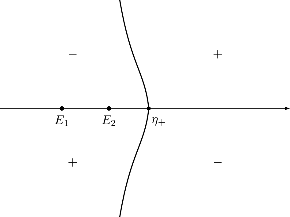
It is readily seen that the \(k\)-derivative of \(g_{\mathrm{\uppercase{\romannumeral1}}}\) is given by \[\label{g95139} g_{\mathrm{\uppercase{\romannumeral1}}}'(k)=\frac{4\left(k-\eta_-(\xi)\right)\left(k-\eta_+(\xi)\right)}{X(k)},\tag{27}\] where \[\begin{align} \eta_+(\xi)=-\frac{4\beta+\xi}{8}+\sqrt{\frac{\alpha^2}{2}+\left(\frac{4\beta-\xi}{8}\right)^2}>E_2,\quad \eta_-(\xi)=-\frac{4\beta+\xi}{8}-\sqrt{\frac{\alpha^2}{2}+\left(\frac{4\beta-\xi}{8}\right)^2}\in(E_1,E_2). \end{align}\] In the transition region \(\mathcal{T}_{\mathrm{\uppercase{\romannumeral1}}}\), saddle point \(\eta_+(\xi)\) tends to \(E_2\) with at least the speed of \(\mathcal{O}(t^{-\frac{2}{3}})\) as \(t\to+\infty\). The signature table for \(\mathop{\mathrm{Im}}g_{\mathrm{\uppercase{\romannumeral1}}}\) is illustrated in Figure 2.
3.1.1 RH problem for \(M^{(1)}\)↩︎
By the function \(g_{\mathrm{\uppercase{\romannumeral1}}}\) defined in 26 , we introduce a new matrix-valued function \(M^{(1)}\) by \[\label{def:M132RI} M^{(1)}(k)= M^{(1)}(k;x,t):=\mathrm{e}^{-\mathrm{i}tg_{\mathrm{\uppercase{\romannumeral1}},\infty}(\xi)\sigma_3}M(k)\mathrm{e}^{\mathrm{i}t\left(g_{\mathrm{\uppercase{\romannumeral1}}}(k)-\theta(k)\right)\sigma_3}.\tag{28}\] Then the RH problem for \(M^{(1)}\) reads as follows:
RH problem 2.
\(M^{(1)}(k)\) is holomorphic for \(k\in\mathbb{C}\setminus\mathbb{R}\).
\(M^{(1)}(k)\) has continuous boundary values \(M_{\pm}^{(1)}(k)\) on \(\mathbb{R}\) with the jump condition \[M^{(1)}_{+}(k)=M^{(1)}_{-}(k)V^{(1)}(k), \quad k\in\mathbb{R},\] where \[\label{equ:jump32V132RI} V^{(1)}(k)= \begin{cases} \begin{pmatrix}1-r(k)r^*(k) & r^*(k)\mathrm{e}^{-2\mathrm{i}tg_{\mathrm{\uppercase{\romannumeral1}}}(k)}\\ -r(k)\mathrm{e}^{2\mathrm{i}tg_{\mathrm{\uppercase{\romannumeral1}}}(k)} & 1\end{pmatrix}, &k\in\mathbb{R}\setminus[E_1,E_2], \\ \begin{pmatrix}0 & r^*(k)\\- r(k) & \mathrm{e}^{-2\mathrm{i}tg_{\mathrm{\uppercase{\romannumeral1}},+}(k)} \end{pmatrix}, &k\in[E_1,E_2]. \end{cases}\qquad{(9)}\]
As \(k\rightarrow\infty\) in \(\mathbb{C}\setminus\mathbb{R}\), we have \(M^{(1)}(k)=I+\mathcal{O}(k^{-1})\).
3.2 Second transformation: \(M^{(1)}\rightarrow M^{(2)}\)↩︎
In this section, we introduce an auxiliary function \(D_{\mathrm{\uppercase{\romannumeral1}}}\) to pave the way for the subsequent contour deformation along the rays \((-\infty, E_1)\) and \((\eta_+, +\infty)\). Moreover, we need to keep the segments \([E_2,\eta_+]\) on the line.
3.2.1 The \(D_{\mathrm{\uppercase{\romannumeral1}}}\) function↩︎
Define \(D_{\mathrm{\uppercase{\romannumeral1}}}: \mathbb{C}\setminus\left((-\infty,E_1]\cup[E_1,E_2]\right) \times \mathcal{T}_{\mathrm{\uppercase{\romannumeral1}}}\to\mathbb{C}\) by \[\label{equ:def32D32function32RI} \begin{align} D_{\mathrm{\uppercase{\romannumeral1}}}(k)=D_{\mathrm{I}}(k;\xi):=\exp\left[\frac{X(k)}{2\pi \mathrm{i}} \left(\int_{-\infty}^{E_1}\frac{\log \left(1-r(z)r^*(z)\right)}{X(z)(z-k)}\mathop{}\!\mathrm{d}z+\int_{E_1}^{E_2} \frac{\log r(z)}{X_{+}(z)(z-k)}\mathop{}\!\mathrm{d}z\right)\right], \end{align}\tag{29}\] where the branch of the function \(\log r(z)\) is such that it is continuous for \(z\in[E_1,E_2]\) and the principal branch is used for \(\log r(E_1)\). The necessary properties of the function \(D_{\mathrm{\uppercase{\romannumeral1}}}\) are given as follows.
Proposition 6. The function \(D_{\mathrm{\uppercase{\romannumeral1}}}\) defined in 29 satisfies the following properties for \(\xi\in \mathcal{T}_{\mathrm{\uppercase{\romannumeral1}}}\):
\(D_{\mathrm{\uppercase{\romannumeral1}}}(k)\) is holomorphic for \(k\in \mathbb{C}\setminus((-\infty,E_1]\cup[E_1,E_2])\).
\(D_{\mathrm{\uppercase{\romannumeral1}}}(k)\) satisfies the following jump relations: \[\begin{align} & D_{\mathrm{\uppercase{\romannumeral1}}, +}(k)=D_{\mathrm{\uppercase{\romannumeral1}}, -}(k)\left(1-r(k)r^*(k)\right), &&k\in (-\infty,E_1),\\ & D_{\mathrm{\uppercase{\romannumeral1}}, +}(k)D_{\mathrm{\uppercase{\romannumeral1}}, -}(k)=r(k), &&k\in (E_1,E_2). \end{align}\]
\(D_{\mathrm{\uppercase{\romannumeral1}}}(k)\) admits the symmetry: \(D_{\mathrm{\uppercase{\romannumeral1}}}(k)D^*_{\mathrm{\uppercase{\romannumeral1}}}(k)=1\) for \(k\in\mathbb{C}\setminus(-\infty,E_1)\). In particular, \(D_{\mathrm{\uppercase{\romannumeral1}},+}(k)\overline{D_{\mathrm{\uppercase{\romannumeral1}},-}(k)}=1\) for \(k\in(-\infty,E_2)\setminus\{E_1\}\).
As \(k\rightarrow \infty\), \[D^{\pm 1}_{\mathrm{\uppercase{\romannumeral1}}}(k)=D^{\pm 1}_{\mathrm{\uppercase{\romannumeral1}},\infty}(\xi)+\mathcal{O}(k^{-1})\] uniformly for all \(\xi\in\mathcal{T}_{\mathrm{\uppercase{\romannumeral1}}}\), where \[D_{\mathrm{\uppercase{\romannumeral1}},\infty}(\xi)=\exp\left[-\frac{1}{2\pi \mathrm{i}} \left(\int_{-\infty}^{E_1}\frac{\log \left(1-r(z)r^*(z)\right)}{X(z)}\mathop{}\!\mathrm{d}z+\int_{E_1}^{E_2} \frac{\log r(z)}{X_{+}(z)}\mathop{}\!\mathrm{d}z\right)\right]\] with \(| D_{\mathrm{\uppercase{\romannumeral1}},\infty}(\xi)|=1\) for all \(\xi\in\mathcal{T}_{\mathrm{\uppercase{\romannumeral1}}}\).
At the branch point \(E_2\), we have: \[\label{equ:singular32behavior32of32D} D_{\mathrm{\uppercase{\romannumeral1}}}(k)=\mathrm{e}^{\frac{\mathrm{i}}{2}\arg q_{2,0}}\left[1+\mathcal{O}\left((k-E_2)^{1/2}\right)\right], \quad k\to E_2.\qquad{(10)}\]
Proof.
It follows from the definition of \(D_{\mathrm{\uppercase{\romannumeral1}}}\) by considering basic ideas of the Cauchy transformation.
The jump condition is an immediate consequence by using the well-known Sokhotski-Plemelj formula.
It can be straightforward verified from the properties of \(r(k)\) in Proposition 4.
It can be readily obtained from the definition of \(D_{\mathrm{\uppercase{\romannumeral1}}}\) in 29 .
From item (d) of Proposition 4, we know that \[\log r(z)=\log q_{2,0}+\mathrm{i}\frac{q_{2,1}}{q_{2,0}}\sqrt{E_2-z}+\mathcal{O}(E_2-z),\quad k\to E_2,\] which implies that \[\begin{align} \int_{E_1}^{E_2}\frac{\log r_{+}(z)}{X_{+}(z)(z-k)}\mathop{}\!\mathrm{d}z=\frac{\pi \log q_{2,0}\mathrm{i}}{\sqrt{E_2-E_1}}(k-E_2)^{-\frac{1}{2}}+\mathcal{O}(1),\quad k\to E_2. \end{align}\] Combined with the asymptotics of \(X(k)\) as \(k\to E_2\), the asymptotics of ?? can be obtained immediately.
◻
3.2.2 RH problem for \(M^{(2)}\)↩︎
With the help of \(D_{\mathrm{\uppercase{\romannumeral1}}}\) function, we define \[\label{def:M232RI} M^{(2)}(k)= M^{(2)}(k;x,t):= D_{\mathrm{\uppercase{\romannumeral1}},\infty}(\xi)^{\sigma_3}M^{(1)}(k)D_{\mathrm{\uppercase{\romannumeral1}}}^{-\sigma_3}(k).\tag{30}\] Then RH problem for \(M^{(2)}\) reads as follows:
RH problem 3.
\(M^{(2)}(k)\) is holomorphic for \(k\in\mathbb{C}\setminus\mathbb{R}\).
\(M^{(2)}(k)\) has continuous boundary values \(M_{\pm}^{(2)}(k)\) on \(\mathbb{R}\) with the jump condition \[M^{(2)}_{+}(k)=M^{(2)}_{-}(k)V^{(2)}(k),\] where \[V^{(2)}(k)= \begin{cases} \begin{pmatrix} 1&D_{\mathrm{\uppercase{\romannumeral1}},+}^2(k)r_2(k)\mathrm{e}^{-2\mathrm{i}tg_\mathrm{\uppercase{\romannumeral1}}(k)}\\-D_{\mathrm{\uppercase{\romannumeral1}},-}^{-2}(k)r^*_2(k)\mathrm{e}^{2\mathrm{i}tg_\mathrm{\uppercase{\romannumeral1}}(k)}&1-r(k)r^*(k) \end{pmatrix},&k\in(-\infty,E_1),\\ \begin{pmatrix}0 & 1\\ -1 & D_{\mathrm{ \uppercase{\romannumeral1}}, +}(k)D_{\mathrm{\uppercase{\romannumeral1}}, -}^{-1}(k)\mathrm{e}^{-2\mathrm{i}tg_{\mathrm{\uppercase{\romannumeral1}},+}(k)} \end{pmatrix}, &k\in (E_1,E_2),\\ \begin{pmatrix}1-r(k)r^*(k) & D_{\mathrm{\uppercase{\romannumeral1}}}^2(k)r^*(k)\mathrm{e}^{-2\mathrm{i}tg_\mathrm{\uppercase{\romannumeral1}}(k)}\\ -D_{\mathrm{\uppercase{\romannumeral1}}}^{-2}(k)r(k)\mathrm{e}^{2\mathrm{i}tg_\mathrm{\uppercase{\romannumeral1}}(k)} & 1\end{pmatrix}, &k\in(E_2,+\infty). \end{cases}\]
As \(k\rightarrow\infty\) in \(\mathbb{C}\setminus\mathbb{R}\), we have \(M^{(2)}(k)=I+\mathcal{O}(k^{-1})\).
3.3 Third transformation: \(M^{(2)}\rightarrow M^{(3)}\)↩︎
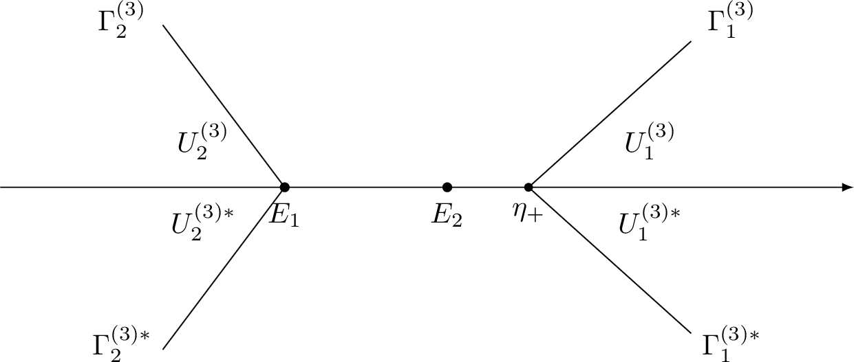
The aim of the third transformation is to open lenses in regions \(U^{(3)}_j,U^{(3)*}_j,\;j=1,2\), which are illustrated in Figure 3. To this end, we need to construct the analytic approximation for the spectral functions \(r(k)\).
3.3.1 Analytic approximation↩︎
The following two proposition establish the analytic approximations for \(r\) and \(r_2\) in different regions as illustrated in Figure 3. Their proofs are analogous to those of Lemma 5.2 and Lemma 5.3 in [48], respectively, and thus are omitted here.
Proposition 7 (Analytic approximation of \(r\)). There exist continuous functions \[r_a: \overline{U_1^{(3)}} \times \mathcal{T}_\mathrm{\uppercase{\romannumeral1}} \rightarrow \mathbb{C} \; \text{ and } \; r_r: (\eta_+,+\infty) \times \mathcal{T}_\mathrm{\uppercase{\romannumeral1}}\rightarrow \mathbb{C},\] which satisfy the following properties:
\(r(k)=r_a(k)+r_r(k)\), where \(r_a(k)=r_a(k;\xi)\) and \(r_r(k)=r_r(k;\xi)\) for all \((k;\xi) \in (\eta_+,+\infty) \times \mathcal{T}_\mathrm{\uppercase{\romannumeral1}}\).
For all \(\xi \in \mathcal{T}_\mathrm{\uppercase{\romannumeral1}}\), the function \(r_a: U_1^{(3)} \rightarrow \mathbb{C}\) is holomorphic. Moreover, for \((k;\xi)\in \overline{U_1^{(3)}} \times \mathcal{T}_\mathrm{\uppercase{\romannumeral1}}\), we have \[\left|r_a(k)-r\left( \eta_+\right)\right| \lesssim \left|k- \eta_+\right| \mathrm{e}^{\frac{t}{4}|\operatorname{Im} g_\mathrm{\uppercase{\romannumeral1}}(k)|},\] and \[\left|r_a(k)\right| \lesssim \frac{\mathrm{e}^{\frac{t}{4}|\operatorname{Im} g_\mathrm{\uppercase{\romannumeral1}}(k)|}}{1+|k|^2}.\]
For all \(\xi \in \mathcal{T}_\mathrm{\uppercase{\romannumeral1}}\), the function \(r_r \in L^p\left(\eta_+,+\infty\right),\; p\in[1,+\infty]\), and as \(t \rightarrow +\infty\), \[\left\|r_r(k)\right\|_{L^p\left(\eta_+,+\infty\right)} = \mathcal{O}\left(t^{-1}\right).\]
Proposition 8 (Analytic approximation of \(r_2\)). There exist continuous functions \[r_{2, a}: \left(\overline{U_2^{(3)}} \backslash\left\{E_1\right\} \right)\times\mathcal{T}_\mathrm{\uppercase{\romannumeral1}} \rightarrow \mathbb{C} \; \text{ and } \; r_{2, r}: \left(-\infty, E_1\right)\times\mathcal{T}_\mathrm{\uppercase{\romannumeral1}} \rightarrow \mathbb{C},\] which satisfy the following properties:
\(r_2(k)=r_{2, a}(k;\xi)+r_{2,r}(k;\xi)\), where \(r_2(k)=r_2(k;\xi)\) and \(r_{2,r}(k)=r_{2,r}(k;\xi)\) for all \((k;\xi) \in \left(-\infty, E_1\right)\times\mathcal{T}_\mathrm{\uppercase{\romannumeral1}}\).
For all \(\xi\in \mathcal{T}_\mathrm{\uppercase{\romannumeral1}}\), the function \(r_{2, a}: U_2^{(3)} \rightarrow \mathbb{C}\) is holomorphic, and \(r_{2, a}(k;\xi)= \mathcal{O}\left(\left|k- E_1\right|^{-1 / 2}\right)\) as \(k \rightarrow E_1\) respectively. Moreover, for every \(\varepsilon>0\), there exists a constant \(C(\varepsilon)>0\) such that for \((k;\xi)\in \left(\overline{U^{(3)}_2}\setminus D_{\varepsilon}(E_1)\right)\times\mathcal{T}_\mathrm{\uppercase{\romannumeral1}}\), we have \[\left|r_{2, a}(k;\xi)\right| \leqslant C(\varepsilon )\frac{\mathrm{e}^{t\left|\operatorname{Im} g_{\mathrm{\uppercase{\romannumeral1}},+}(\xi;k)\right|}}{1+|k|^2}.\]
For all \(\xi\in \mathcal{T}_\mathrm{\uppercase{\romannumeral1}}\), the function \(r_{2, r} \in L^p \left(-\infty, E_1\right),\;p\in[1,+\infty]\), and as \(t \rightarrow +\infty\), \[\left\|r_{2, r}(k;\xi)\right\|_{L^p\left(-\infty, E_1\right)} = \mathcal{O}\left(t^{-1}\right).\]
3.3.2 RH problem for \(M^{(3)}\)↩︎
Now we are ready to introduce a transformation \[\label{def:M332RI} M^{(3)}(k)=M^{(3)}(k;x,t):=M^{(2)}(k)D_{\mathrm{\uppercase{\romannumeral1}}}^{\sigma_3}(k)G(k)D_{\mathrm{\uppercase{\romannumeral1}}}^{-\sigma_3}(k),\tag{31}\] where \[\label{def:G40k4132T1} G(k):= \begin{cases} \begin{pmatrix}1 & 0 \\ r_a\mathrm{e}^{2\mathrm{i}tg_{\mathrm{\uppercase{\romannumeral1}}}} & 1\end{pmatrix}, &k\in U^{(3)}_1, \\ \begin{pmatrix}1 & r_a^{*}\mathrm{e}^{-2\mathrm{i}tg_\mathrm{\uppercase{\romannumeral1}}} \\ 0 & 1\end{pmatrix}, &k\in U_1^{(3)*}, \\ \begin{pmatrix}1 & -r_{2,a}\mathrm{e}^{-2\mathrm{i}tg_\mathrm{\uppercase{\romannumeral1}}} \\ 0 & 1\end{pmatrix}, &k\in U_2^{(3)},\\ \begin{pmatrix}1 & 0 \\ -r^*_{2,a}\mathrm{e}^{2\mathrm{i}tg_\mathrm{\uppercase{\romannumeral1}}} & 1\end{pmatrix}, & k\in U_2^{(3)*},\\ I, &\textrm{elsewhere}. \end{cases}\tag{32}\] Here, the domains \(U^{(3)}_j\) for \(j=1,2\) are illustrated in Figure 3.
Then RH problem for \(M^{(3)}\) reads as follows:
RH problem 4.
\(M^{(3)}(k)\) is holomorphic for \(k\in\mathbb{C}\backslash\Gamma^{(3)}\), where \(\Gamma^{(3)}:=\cup_{j=1}^{2}(\Gamma^{(3)}_j\cup\Gamma_j^{(3)*})\cup\mathbb{R}\); see Figure 3 for an illustration.
\(M^{(3)}(k)\) has continuous boundary values \(M_{\pm}^{(3)}(k)\) on \(k\in \Gamma^{(3)}\) with the jump condition \[M^{(3)}_{+}(k)= M^{(3)}_{-}(k)V^{(3)}(k),\] where \[\label{equ:jump32V332RI} V^{(3)}(k)= \begin{cases} \begin{pmatrix} 1 & 0\\ -D_{\mathrm{\uppercase{\romannumeral1}}}^{-2}(k)r_a(k)\mathrm{e}^{2\mathrm{i}tg_\mathrm{\uppercase{\romannumeral1}}(k)} & 1\end{pmatrix}, &k\in\Gamma^{(3)}_1, \\ \begin{pmatrix} 1 & D_{\mathrm{\uppercase{\romannumeral1}},+}^{2}(k)r_{2,a}(k)\mathrm{e}^{-2\mathrm{i}tg_\mathrm{\uppercase{\romannumeral1}}(k)}\\ 0& 1\end{pmatrix}, &k\in\Gamma^{(3)}_2, \\ \begin{pmatrix} 1 & D_{\mathrm{\uppercase{\romannumeral1}}}^{2}(k)r_a^*(k)\mathrm{e}^{-2\mathrm{i}tg_\mathrm{\uppercase{\romannumeral1}}(k)}\\ 0 & 1\end{pmatrix}, & k\in\Gamma^{(3)*}_1, \\ \begin{pmatrix} 1 & 0\\ -D_{\mathrm{\uppercase{\romannumeral1}},-}^{-2}(k)r_{2,a}^*(k)\mathrm{e}^{2\mathrm{i}tg_\mathrm{\uppercase{\romannumeral1}}(k)} & 1\end{pmatrix}, & k\in\Gamma^{(3)*}_2, \\ \begin{pmatrix} 1-r_r(k)r^*_r(k)&D_\mathrm{\uppercase{\romannumeral1}}^2(k)r_r^*(k)\mathrm{e}^{-2\mathrm{i}tg_\mathrm{\uppercase{\romannumeral1}}(k)}\\-D_\mathrm{\uppercase{\romannumeral1}}^{-2}(k)r_r(k)\mathrm{e}^{2\mathrm{i}tg_\mathrm{\uppercase{\romannumeral1}}(k)}&1 \end{pmatrix},&k\in(\eta_+,+\infty),\\ \begin{pmatrix} 1&D_\mathrm{\uppercase{\romannumeral1},+}^2(k)r_{2,r}(k)\mathrm{e}^{-2\mathrm{i}tg_\mathrm{\uppercase{\romannumeral1}}(k)}\\-D_{\mathrm{\uppercase{\romannumeral1}},-}^{-2}(k)r^*_{2,r}(k)\mathrm{e}^{2\mathrm{i}tg_\mathrm{\uppercase{\romannumeral1}}(k)}&1-r_r(k)r^*_r(k) \end{pmatrix},&k\in(-\infty,E_1),\\ \begin{pmatrix}1-r(k)r^*(k) & D_{\mathrm{\uppercase{\romannumeral1}}}^2(k)r^*(k)\mathrm{e}^{-2\mathrm{i}tg_\mathrm{\uppercase{\romannumeral1}}(k)}\\ -D_{\mathrm{\uppercase{\romannumeral1}}}^{-2}(k)r(k)\mathrm{e}^{2\mathrm{i}tg_\mathrm{\uppercase{\romannumeral1}}(k)} & 1\end{pmatrix},&k\in(E_2,\eta_+),\\ \begin{pmatrix} 0&1\\-1&D_{\mathrm{\uppercase{\romannumeral1}},+}(k)D_{\mathrm{\uppercase{\romannumeral1}},-}^{-1}(k)\mathrm{e}^{-2\mathrm{i}tg_{\mathrm{\uppercase{\romannumeral1}},+}(k)}\\ \end{pmatrix},&k\in(E_1,E_2). \end{cases}\qquad{(11)}\]
As \(k\rightarrow\infty\) in \(\mathbb{C}\setminus\Gamma^{(3)}\), we have \(M^{(3)}(k)=I+\mathcal{O}(k^{-1})\).
3.4 Analysis of RH problem for \(M^{(3)}\)↩︎
It is readily seen that \(V^{(3)} \to I\) exponentially on the contours \(\Gamma^{(3)}_j \cup \Gamma_j^{(3)*}\) for \(j=1,2\) as \(t \to +\infty\) except around the point \(\eta_+\), which tends to \(E_2\) as \(t\) large. Item (c) of Proposition 7 and item (c) of Proposition 8 ensure that \(V^{(3)} \to I\) on intervals \((-\infty,E_1)\) and \((\eta_+,+\infty)\). These two facts lead us to consider the following global parametrix.
3.4.1 Global parametrix↩︎
For \(\xi \in \mathcal{T}_\mathrm{\uppercase{\romannumeral1}}\), the global parametrix \(M^{(\infty)}(k)\) satisfies the following RH problem.
RH problem 5.
\(M^{(\infty)}(k)\) is holomorphic for \(k\in\mathbb{C}\setminus[E_1,E_2]\).
\(M^{(\infty)}(k)\) has continuous boundary values \(M_{\pm}^{(\infty)}(k)\) on \((E_1,E_2)\) satisfying the following jump condition: \[\begin{align} M_{+}^{(\infty)}(k)=M_{-}^{(\infty)}(k)V^{(\infty)}(k), \end{align}\] where \[V^{(\infty)}(k)=\begin{pmatrix} 0 & 1\\ -1 & 0 \end{pmatrix}.\]
As \(k\rightarrow\infty\) in \(\mathbb{C}\setminus[E_1,E_2]\), we have \(M^{(\infty)}(k)=I+\mathcal{O}(k^{-1})\).
As \(k\rightarrow E_j\) for \(j=1,2\), \(M^{(\infty)}(k)=\mathcal{O}((k- E_j)^{-1/4})\).
Lemma 1. The RH problem 5 has a unique solution which is given by \[\label{equ:sol32of32Minfty} M^{(\infty)}(k)=\frac{1}{2} \left( \begin{array}{cc} \chi(k)+\chi^{-1}(k) & -\mathrm{i}\left(\chi(k)-\chi^{-1}(k)\right)\\ \mathrm{i}\left(\chi(k)-\chi^{-1}(k)\right) & \chi(k)+\chi^{-1}(k) \end{array} \right),\qquad{(12)}\] where \(\chi(k)\) is defined as in 12 . Moreover, for \(\xi \in \mathcal{T}_\mathrm{\uppercase{\romannumeral1}}\), the following expansions hold true for \(M^{(\infty)}\):
As \(k\rightarrow\infty\) in \(\mathbb{C}\setminus[E_1,E_2]\), \[M^{(\infty)}(k)=I+\frac{1}{k}\begin{pmatrix} 0&\frac{\mathrm{i}\alpha}{2}\\-\frac{\mathrm{i}\alpha}{2}&0 \end{pmatrix}+\frac{1}{k^2}\begin{pmatrix} \frac{\alpha^2}{8}&-\frac{\mathrm{i}\alpha\beta}{2}\\\frac{\mathrm{i}\alpha\beta}{2}&\frac{\alpha^2}{8} \end{pmatrix}+\mathcal{O}(k^{-3}).\]
As \(k\rightarrow E_2\), \[\begin{align} M^{(\infty)}(k)&= \frac{\left(2\alpha\right)^{1 / 4}}{2\left(k-E_2\right)^{1 / 4}}\left\{\begin{pmatrix} 1 & \mathrm{i}\\ -\mathrm{i}& 1 \end{pmatrix}+\frac{\left(k-E_2\right)^{1 / 2}}{\left(2\alpha\right)^{1 / 2}}\begin{pmatrix} 1 & -\mathrm{i}\\ \mathrm{i}& 1 \end{pmatrix}+\frac{k-E_2}{8\alpha}\begin{pmatrix} 1 & \mathrm{i}\\ -\mathrm{i}& 1 \end{pmatrix}\right. \\ & \left.+\frac{\left(k-E_2\right)^{3 / 2}}{4\left(2\alpha\right)^{3 / 2}}\begin{pmatrix} -1 & \mathrm{i}\\ -\mathrm{i}& -1 \end{pmatrix}+\mathcal{O}\left(\left|k-E_2\right|^2\right)\right\}. \end{align}\]
3.4.2 Local parametrix near \(E_2\)↩︎
Let \[\begin{align} \label{def32local} D_\varrho(E_2)=\left\{k: |k-E_2|<\varrho \right\} \end{align}\tag{33}\] be a small disk around \(E_2\), where \[\varrho<{\rm min}\left\{2 |\eta_+-E_2|t^{\epsilon_1}, \frac{1}{3} |\eta_+|,\frac{2\alpha}{3} \right\}, \quad \frac{1}{2}<\epsilon_1<\frac{2}{3}.\] We intend to solve the following local RH problem for \(M^{(loc)}\).
RH problem 6.
\(M^{(loc)}(k)\) is holomorphic for \(k\in\overline{D_{\varrho}( E_2)}\setminus\Gamma^{(loc)}\) , where \[\begin{align} \label{def:Gamma9440ell4132RI} \Gamma^{(loc)}:=D_\varrho(E_2)\cap \Gamma^{(3)}. \end{align}\qquad{(13)}\]
\(M^{(loc)}(k)\) has continuous boundary values \(M_{\pm}^{(loc)}(k)\) on \(k\in \Gamma^{(loc)}\) with the jump condition \[\begin{align} M^{(loc)}_{+}(k)=M^{(loc)}_{-}(k)V^{(3)}(k)\big|_{\Gamma^{(loc)}}, \end{align}\] where \(V^{(3)}(k)\) is given by ?? .
As \(k\rightarrow\infty\) in \(\mathbb{C}\setminus\Gamma^{(loc)}\), we have \(M^{(loc)}(k)=I+\mathcal{O}(k^{-1})\).
The solution \(M^{(loc)}\) for this local RH problem can be constructed by the Painlevé XXXIV parametrix shown in Appendix 6 in a standard manner. In the rest part of this section, we focus on the construction of \(M^{(loc)}\) near \(k=E_2\).
First, we introduce the following change of variables. Recall the asymptotics of \(g_{\mathrm{\uppercase{\romannumeral1}}}\) in ?? that \[g_{\mathrm{\uppercase{\romannumeral1}}}(k)=g_{\mathrm{\uppercase{\romannumeral1}}}^{(1)}(E_2)(k- E_2)^{\frac{1}{2}}+g_{\mathrm{\uppercase{\romannumeral1}}}^{(2)}(E_2)(k- E_2)^{\frac{3}{2}}+\mathcal{O}((k- E_2)^{\frac{5}{2}}),\quad k\to E_2,\] where \[\label{equ:coefficients32of32gI} g_{\mathrm{\uppercase{\romannumeral1}}}^{(1)}(E_2)=2\alpha(\xi+2\alpha-4\beta),\quad g_{\mathrm{\uppercase{\romannumeral1}}}^{(2)}(E_2)=\frac{\xi+2\alpha-4\beta}{2\sqrt{2\alpha}}+4\alpha.\tag{34}\]
For \((k;\xi)\in \left( D_{\varrho}(E_2)\setminus(-\infty,E_2] \right)\times \mathcal{T}_\mathrm{\uppercase{\romannumeral1}}\), it can be readily seen that \(g_{\mathrm{\uppercase{\romannumeral1}}}^{(1)}(E_2)=\mathcal{O}(t^{-2/3})\), thus we have \[\label{asy32ImgI} \mathrm{Im} g_{\mathrm{\uppercase{\romannumeral1}}}(k)\lesssim \pm t^{-2/3}\left|k- E_2\right|^{\frac{1}{2}},\quad k\in \left(D_{\varrho}(E_2)\setminus(-\infty,E_2]\right)\cap\mathbb{C}_{\pm}.\tag{35}\]
For \(k \in D_{\varrho}(E_2)\setminus(-\infty,E_2]\), we set \[\label{vira32cha321} \zeta(k) :=-\left(\frac{3}{2}\right)^{\frac{2}{3}}t^{\frac{2}{3}}\left[g_{\mathrm{\uppercase{\romannumeral1}}}(k)-g_{\mathrm{\uppercase{\romannumeral1}}}^{(1)}(E_2)(k-E_2)^{\frac{1}{2}}\right]^{\frac{2}{3}},\tag{36}\] where the cut \((\cdot)^{\frac{3}{2}}\) runs along \(\mathbb{R}^{-}\). This is a one-to-one conformal mapping form \(k\)-plane to \(\zeta\)-plane as \(\zeta^\prime(E_2)=-\left(\frac{3}{2}\right)^{\frac{2}{3}}t^{\frac{2}{3}}\left|g_{\mathrm{\uppercase{\romannumeral1}}}^{(2)}(E_2)\right|^{\frac{2}{3}}<0\). Moreover, we have \[\label{asy32zeta1472} \zeta(k)^{\frac{1}{2}}=\begin{cases} -\mathrm{i}t^{\frac{1}{3}}(\frac{3}{2})^{\frac{1}{3}}\left|g_{\mathrm{\uppercase{\romannumeral1}}}^{(2)}(E_2)\right|^{\frac{1}{3}}(k-E_2)^{\frac{1}{2}}\left(1+\mathcal{O}(k-E_2)\right),&k \to E_2,\;k \in \mathbb{C}^+,\\ \mathrm{i}t^{\frac{1}{3}}(\frac{3}{2})^{\frac{1}{3}}\left|g_{\mathrm{\uppercase{\romannumeral1}}}^{(2)}(E_2)\right|^{\frac{1}{3}}(k-E_2)^{\frac{1}{2}}\left(1+\mathcal{O}(k-E_2)\right),&k \to E_2,\;k \in \mathbb{C}^-, \end{cases}\tag{37}\] as well as \[\label{asy32zeta323472} \zeta(k)^{\frac{3}{2}}=\begin{cases} \frac{3\mathrm{i}}{2}tg_{\mathrm{\uppercase{\romannumeral1}}}^{(2)}(E_2)(k-E_2)^{\frac{3}{2}}\left(1+\mathcal{O}(k-E_2)\right),&k \to E_2,\;k \in \mathbb{C}^+,\\ -\frac{3\mathrm{i}}{2}tg_{\mathrm{\uppercase{\romannumeral1}}}^{(2)}(E_2)(k-E_2)^{\frac{3}{2}}\left(1+\mathcal{O}(k-E_2)\right),&k \to E_2,\;k \in \mathbb{C}^-. \end{cases}\tag{38}\] Then we define \[S(k)= S(k;\xi):=\begin{cases} \mathrm{i}t\frac{g_{\mathrm{\uppercase{\romannumeral1}}}^{(1)}(E_2)(k-E_2)^{\frac{1}{2}}}{\zeta(k)^{\frac{1}{2}}}, &k\in D_{\varrho}(E_2)\cap\mathbb{C}^+,\\ - \mathrm{i}t\frac{g_{\mathrm{\uppercase{\romannumeral1}}}^{(1)}(E_2)(k-E_2)^{\frac{1}{2}}}{\zeta(k)^{\frac{1}{2}}}, &k\in D_{\varrho}(E_2)\cap\mathbb{C}^-. \end{cases}\] From 37 we know that \(S(k)\) is analytic in \(D_{\varrho}(E_2)\) and define \[\label{defS} s:=S(E_2)=-t^{\frac{2}{3}}\frac{g_{\mathrm{\uppercase{\romannumeral1}}}^{(1)}(E_2)}{\left(\frac{3}{2}\right)^{\frac{1}{3}}\left|g_{\mathrm{\uppercase{\romannumeral1}}}^{(2)}(E_2)\right|^{\frac{1}{3}}}.\tag{39}\] It can be concluded from 37 , 38 and 39 that \[\frac{4}{3}\zeta(k)^{\frac{3}{2}}+2S(k)\zeta(k)^{\frac{1}{2}}=\begin{cases} 2\mathrm{i}tg_{\mathrm{\uppercase{\romannumeral1}}}(k), &k\in D_{\varrho}(E_2)\cap\mathbb{C}^+,\\ -2\mathrm{i}tg_{\mathrm{\uppercase{\romannumeral1}}}(k), &k\in D_{\varrho}(E_2)\cap\mathbb{C}^-. \end{cases}\]
To match \(M^{(loc)}\) near \(E_2\), the change of variable from \(k\)-plane to \(\zeta\)-plane in 36 inspires us to consider the problem in \(\zeta\)-plane which maps \(E_2\) to the origin. Let \(\widehat D_{\varrho}:=\zeta(D_{\varrho}(E_2)),\; \widehat\Gamma_1:=\zeta(\Gamma^{(3)*}_1),\;\widehat \Gamma^{(loc)}:=\zeta(\Gamma^{(loc)})\).
Therefore, we can define by \(\widehat M^{(loc)}(\zeta):=M^{(loc)}(k(\zeta))\) with the jump condition \(\widehat M^{(loc)}_+(\zeta)=\widehat M^{(loc)}_-(\zeta)\widehat V^{(3)}(\zeta)\) on \(\widehat\Gamma^{(loc)}\), where \[\label{equ:jump32zetar} \widehat V^{(3)}(\zeta)\big|_{\widehat\Gamma^{(loc)}}= \begin{cases} \begin{pmatrix} 1 & -D_{\mathrm{\uppercase{\romannumeral1}}}^{2}(k(\zeta))r_a^*(k(\zeta))\mathrm{e}^{-2\mathrm{i}tg_\mathrm{\uppercase{\romannumeral1}}(k(\zeta))}\\ 0 & 1\end{pmatrix}, & \zeta\in\widehat\Gamma^{(loc)}_1, \\ \begin{pmatrix} 1 & 0\\ D_{\mathrm{\uppercase{\romannumeral1}}}^{-2}(k(\zeta))r_a(k(\zeta))\mathrm{e}^{2\mathrm{i}tg_\mathrm{\uppercase{\romannumeral1}}(k(\zeta))} & 1\end{pmatrix}, &\zeta\in\widehat\Gamma^{(loc)*}_1, \\ \begin{pmatrix} 1&-D_\mathrm{\uppercase{\romannumeral1}}^2(k(\zeta))r_r^*(k(\zeta))\mathrm{e}^{-2\mathrm{i}tg_\mathrm{\uppercase{\romannumeral1}}(k(\zeta))}\\D_\mathrm{\uppercase{\romannumeral1}}^{-2}(k(\zeta))r_r(k(\zeta))\mathrm{e}^{2\mathrm{i}tg_\mathrm{\uppercase{\romannumeral1}}(k(\zeta))}&1-r_r(k(\zeta))r^*_r(k(\zeta)) \end{pmatrix},&\zeta\in(-\varrho,\zeta(\eta_+)),\\ \begin{pmatrix}1 & -D_{\mathrm{\uppercase{\romannumeral1}}}^2(k(\zeta))r^*(k(\zeta))\mathrm{e}^{-2\mathrm{i}tg_\mathrm{\uppercase{\romannumeral1}}(k(\zeta))}\\ D_{\mathrm{\uppercase{\romannumeral1}}}^{-2}(k(\zeta))r(k(\zeta))\mathrm{e}^{2\mathrm{i}tg_\mathrm{\uppercase{\romannumeral1}}(k(\zeta))} & 1-r(k(\zeta))r^*(k(\zeta))\end{pmatrix},&\zeta\in(\zeta(\eta_+),0),\\ \begin{pmatrix} D_{\mathrm{\uppercase{\romannumeral1}},+}(k(\zeta))D_{\mathrm{\uppercase{\romannumeral1}},-}^{-1}(k(\zeta))\mathrm{e}^{-2\mathrm{i}tg_{\mathrm{\uppercase{\romannumeral1}},+}(k(\zeta))}&-1\\1&0 \end{pmatrix},&\zeta\in(0,\varrho). \end{cases}\tag{40}\] See Figure 4.
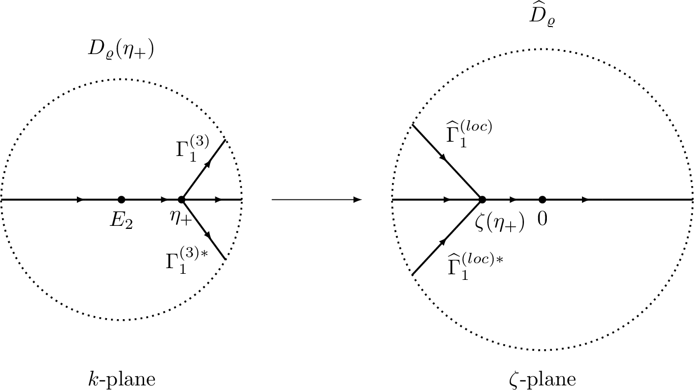
It follows from the definition of \(D_{\varrho}(E_2)\) in 33 that as \(t\to\infty\), we have \[k-E_2=\mathcal{O}(t^{-2/3+\varepsilon_1}),\quad k\in D_{\varrho}(E_2).\] With respect to item (e) of Proposition 6, item (b) of Proposition 7 and the asymptotics of \(r(k)\) near \(E_2\) in Proposition 4, we have, for large \(t\), \[\begin{align} D_{\mathrm{\uppercase{\romannumeral1}}}(k)&=e^{\frac{\mathrm{i}}{2}\arg q_{2,0}}+\mathcal{O}(t^{-1/3+\epsilon_1/2}),\\ |r_a(k)-r(E_2)|&\lesssim|k-E_2|^{1/2}+|k-E_2|\mathrm{e}^{\frac{t}{4}|\mathrm{Im} g_\mathrm{\uppercase{\romannumeral1}}|}\\ &\lesssim t^{-1/3+\epsilon_1/2}+t^{-2/3+\epsilon_1}\mathrm{e}^{\frac{t}{4}|\mathrm{Im} g_\mathrm{\uppercase{\romannumeral1}}|},\quad k\in D_{\varrho}(E_2)\cap\mathbb{C}^+. \end{align}\] which implies that for \(k\in D_{\varrho}(E_2)\cap\mathbb{C}^+\), \[\begin{align} \label{asy1} | D_{\mathrm{\uppercase{\romannumeral1}}}^{-2}(k)r_a(k)-D_{\mathrm{\uppercase{\romannumeral1}}}^{-2}(E_2)r_a(E_2)|=|D_{\mathrm{\uppercase{\romannumeral1}}}^{-2}(k)r_a(k)-1|&\lesssim t^{-1/3+\epsilon_1/2}+t^{-2/3+\epsilon_1}\mathrm{e}^{\frac{t}{4}|\mathrm{Im} g_\mathrm{\uppercase{\romannumeral1}}|}. \end{align}\tag{41}\] Therefore, RH problem \(\widehat M^{(loc)}(\zeta)\) can be approximated by the following RH problem \(\widehat N^{(loc)}(\zeta)\) which is associated with the Painlevé parametrix.
RH problem 7.
\(\widehat N^{(loc)}(\zeta)\) is holomorphic for \(\zeta\in\mathbb{C}\setminus \left(\widehat\Gamma^{(loc)}\setminus(-\infty,\zeta(\eta_+))\right)\).
\(\widehat N^{(loc)}(\zeta)\) has continuous boundary values \(\widehat N^{(loc)}_\pm(\zeta)\) on \(\zeta\in \widehat\Gamma^{(loc)}\setminus(-\infty,\zeta(\eta_+))\) with the jump condition \[\begin{align} \widehat N^{(loc)}_+(\zeta)=\widehat N^{(loc)}_-(\zeta)\widehat V_N^{(loc)}(\zeta), \end{align}\] where \[\label{equ:jumpVN} \widehat V_N^{(loc)}(\zeta)= \begin{cases} \begin{pmatrix} 1 & -\mathrm{e}^{2\hat{\theta}(\zeta)}\\ 0 & 1\end{pmatrix}, & \zeta\in\widehat\Gamma^{(loc)}_1, \\ \begin{pmatrix} 1 & 0\\ \mathrm{e}^{2\hat{\theta}(\zeta)} & 1\end{pmatrix}, &\zeta\in\widehat\Gamma^{(loc)*}_1, \\ \begin{pmatrix} 1 & 0\\ \mathrm{e}^{2\hat{\theta}(\zeta)} & 1\end{pmatrix} \begin{pmatrix} 1 & -\mathrm{e}^{2\hat{\theta}(\zeta)}\\ 0 & 1\end{pmatrix} ,&\zeta\in(\zeta(\eta_+),0),\\ \begin{pmatrix}0 & -1 \\ 1 & 0\end{pmatrix}, & \zeta\in (0,\varrho) \end{cases}\qquad{(14)}\] with \[\label{hattheta} \hat{\theta}(\zeta)=\frac{2}{3}\zeta^{\frac{3}{2}}+s\zeta^{\frac{1}{2}}.\qquad{(15)}\]
Next transformation is used to remove the jump contours \(\widehat\Gamma^{(loc)}_1\) and \(\widehat\Gamma^{(loc)*}_1\) from the starting point \(\zeta(\eta_+)\) to \(0\). Define a matrix function \(G^{(loc)}(\zeta)\) on complex plane \(\zeta\) by \[G^{(loc)}(\zeta)=\begin{cases} \begin{pmatrix} 1 & \mathrm{e}^{2\hat{\theta}(\zeta)}\\ 0 & 1\end{pmatrix}, & \zeta\in\Omega_1,\\ \begin{pmatrix} 1 & 0\\ \mathrm{e}^{2\hat{\theta}(\zeta)} & 1\end{pmatrix}, &\zeta\in\Omega_1^*,\\ I,&\text{elsewhere}. \end{cases}\] Therefore, we can construct a new transformation \[\label{trans32N32to32S} \widehat S^{(loc)}(\zeta)=\widehat N^{(loc)}(\zeta) G^{(loc)}(\zeta),\tag{42}\] which implies that \(\widehat S^{(loc)}(\zeta)\) satisfies the following RH problem
RH problem 8.
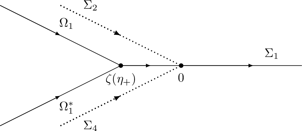
\(\widehat S^{(loc)}(\zeta)\) is holomorphic for \(\zeta\in\mathbb{C}\setminus \cup_{j=1,2,4}\Sigma_j\), where \(\Sigma_j\) for \(j=1,2,4\) is shown in Figure 15.
\(\widehat S^{(loc)}(\zeta)\) has continuous boundary values \(\widehat S^{(loc)}_\pm(\zeta)\) on \(\zeta\in \cup_{j=1,2,4}\Sigma_j\) with the jump condition \[\begin{align} \widehat S^{(loc)}_+(\zeta)=\widehat S^{(loc)}_-(\zeta)\widehat V_S^{(loc)}(\zeta), \end{align}\] where \[\widehat V_S^{(loc)}(\zeta)= \begin{cases} \begin{pmatrix}0 & -1 \\ 1 & 0\end{pmatrix}, & \zeta\in \Sigma_1\\ \begin{pmatrix} 1 & -\mathrm{e}^{2\hat{\theta}(\zeta)}\\ 0 & 1\end{pmatrix}, & \zeta\in\Sigma_2, \\ \begin{pmatrix} 1 & 0\\ \mathrm{e}^{2\hat{\theta}(\zeta)} & 1\end{pmatrix},&\zeta\in\Sigma_4,\\ \end{cases}\]see Figure 5.
With the help of Painlevé XXXIV parametrix defined in Appendix 6, the solution to the RH problem \(\widehat S^{(loc)}(\zeta)\) can be constructed by \[\label{equ:hat32S32trans} \widehat S^{(loc)}(\zeta)=\begin{pmatrix} 1 & 0\\ \mathrm{i}a(s) & 1 \end{pmatrix}M^{P_{34}}\left(\zeta; 0, 0, s\right)\mathrm{e}^{\hat{\theta}(\zeta)\sigma_3}Q(\zeta),\tag{43}\] where \[\label{def:Qr} Q(\zeta)=\begin{cases} \sigma_1 \mathrm{e}^{\frac{\pi\mathrm{i}}{2}\sigma_3},&\zeta\in\mathbb{C}^+,\\ \sigma_3\mathrm{e}^{\frac{\pi\mathrm{i}}{2}\sigma_3},&\zeta\in\mathbb{C}^-. \end{cases}\tag{44}\] Deduced from the asymptotics of \(M^{P_{34}}(\zeta; 0,0,s)\) in ?? , \(\widehat S^{(loc)}(\zeta)\) has the following asymptotics as \(\zeta\to\infty\): \[\label{asy32S} \widehat S^{(loc)}(\zeta)=\left(I+\mathcal{O} \left( \zeta^{-1} \right) \right) \frac{\zeta^{-\frac{1}{4}\sigma_3}}{\sqrt{2}} \begin{pmatrix} 1 & \mathrm{i} \\ \mathrm{i}& 1 \end{pmatrix}Q.\tag{45}\]
Define \(E(\zeta)=\widehat M^{(loc)}(\zeta)\widehat N^{(loc)}(\zeta)^{-1}\), then we can obtain the following RH problem for \(E(\zeta)\).
RH problem 9.
\(E(\zeta)\) is holomorphic for \(k\in\mathbb{C}\setminus \widehat\Gamma^{(loc)}\).
\(E(\zeta)\) has continuous boundary values \(E_\pm(\zeta)\) on \(\widehat\Gamma^{(loc)}\) with the jump condition \[\begin{align} E_+(\zeta)=E_-(\zeta) V_E(\zeta), \end{align}\] where \[V_E(\zeta)=\widehat N^{(loc)}_-(\zeta)\widehat V^{(3)}(\zeta)\widehat V^{(loc)}_N(\zeta)^{-1}\widehat N^{(loc)}_-(\zeta)^{-1}.\]
Proposition 9. For \(\xi\in\mathcal{T}_{\mathrm{\uppercase{\romannumeral1}}}\), as \(t\to+\infty\), \(E(\zeta)\) exists uniquely and satisfies \[\label{esti32for32E} \begin{align} \left\| E(\zeta)-I\right\|_{L^\infty\left(\widehat D_\varrho\right)}&=\mathcal{O}(t^{-\frac{1}{3}-\frac{\epsilon_1}{2}}),\\ \left\| E(\zeta)-I\right\|_{L^1\left(\widehat D_\varrho\right)}&=\mathcal{O}(t^{-1-\frac{\epsilon_1}{2}}),\\ \left\| E(\zeta)-I\right\|_{L^2\left(\widehat D_\varrho\right)}&=\mathcal{O}(t^{-\frac{2}{3}-\frac{\epsilon_1}{2}}). \end{align}\qquad{(16)}\]
Proof. From formulas of \(\widehat V^{(3)}(\zeta)\) in 40 and \(\widehat V_N^{(loc)}(\zeta)\) in ?? , it can be calculated that \[\widehat V^{(3)}(\zeta)\widehat V^{(loc)}_N(\zeta)^{-1}= \begin{cases} \begin{pmatrix} 1 & \mathrm{e}^{2\hat{\theta}}-D_{\mathrm{\uppercase{\romannumeral1}}}^{2}r_a^*\mathrm{e}^{-2\mathrm{i}tg_\mathrm{\uppercase{\romannumeral1}}}\\ 0 & 1\end{pmatrix}, & \zeta\in\widehat\Gamma^{(loc)}_1, \\ \begin{pmatrix} 1 & 0\\ D_{\mathrm{\uppercase{\romannumeral1}}}^{-2}r_a\mathrm{e}^{2\mathrm{i}tg_\mathrm{\uppercase{\romannumeral1}}}-\mathrm{e}^{2\hat{\theta}} & 1\end{pmatrix}, &\zeta\in\widehat\Gamma^{(loc)*}_1, \\ \begin{pmatrix} 1&-D_\mathrm{\uppercase{\romannumeral1}}^2r_r^*\mathrm{e}^{-2\mathrm{i}tg_\mathrm{\uppercase{\romannumeral1}}}\\D_\mathrm{\uppercase{\romannumeral1}}^{-2}r_r\mathrm{e}^{2\mathrm{i}tg_\mathrm{\uppercase{\romannumeral1}}}&1-r_rr^*_r \end{pmatrix},&\zeta\in(-\varrho,\zeta(\eta_+))\\ \begin{pmatrix}1 & -D_{\mathrm{\uppercase{\romannumeral1}}}^2r^*\mathrm{e}^{-2\mathrm{i}tg_\mathrm{\uppercase{\romannumeral1}}}\\ D_{\mathrm{\uppercase{\romannumeral1}}}^{-2}r\mathrm{e}^{2\mathrm{i}tg_\mathrm{\uppercase{\romannumeral1}}} & 1-rr^*\end{pmatrix}\begin{pmatrix} 1 & \mathrm{e}^{2\hat{\theta}}\\ 0 & 1\end{pmatrix} \begin{pmatrix} 1 & 0\\ -\mathrm{e}^{2\hat{\theta}} & 1\end{pmatrix} ,&\zeta\in(\zeta(\eta_+),0),\\ \begin{pmatrix} 1&D_{\mathrm{\uppercase{\romannumeral1}},+}D_{\mathrm{\uppercase{\romannumeral1}},-}^{-1}\mathrm{e}^{-2\mathrm{i}tg_{\mathrm{\uppercase{\romannumeral1}},+}}\\0&1 \end{pmatrix},&\zeta\in(0,\varrho). \end{cases}\]
For \(\zeta\in\widehat\Gamma^{(loc)}_1\), we have that \[\begin{align} \left|\mathrm{e}^{2\hat{\theta}}-D_{\mathrm{\uppercase{\romannumeral1}}}^{2}r_a^*\mathrm{e}^{-2\mathrm{i}tg_\mathrm{\uppercase{\romannumeral1}}}\right|\leqslant\left|\left(D_{\mathrm{\uppercase{\romannumeral1}}}^{2}r_a^*-1\right)\mathrm{e}^{2\hat{\theta}}\right|+\left|D_{\mathrm{\uppercase{\romannumeral1}}}^{2}r_a^*\mathrm{e}^{2\hat{\theta}}\left(\mathrm{e}^{2(S(k)-s)\zeta^{1/2}}-1\right)\right|. \end{align}\] On one hand, 35 and 41 imply that \[\begin{align} \left|\left(D_{\mathrm{\uppercase{\romannumeral1}}}^{2}r_a^*-1\right)\mathrm{e}^{2\hat{\theta}}\right|\lesssim|k-E_2|^{1/2}\mathrm{e}^{-t^{1/3}|k-E_2|^{1/2}} \end{align}\] uniformly for all \(\zeta\in\widehat\Gamma^{(loc)}_1\). Therefore, we can infer that for all \(\xi\in\mathcal{T}_{\mathrm{\uppercase{\romannumeral1}}}\), \[\label{equ:asy32for1} \begin{align} \left\|\left(D_{\mathrm{\uppercase{\romannumeral1}}}^{2}r_a^*-1\right)\mathrm{e}^{2\hat{\theta}}\right\|_{L^1\left(\widehat\Gamma^{(loc)}_1\right)}&\lesssim\int_0^{\varrho}u^{1/2}\mathrm{e}^{-t^{1/3}u^{1/2}}\mathop{}\!\mathrm{d}u=\mathcal{O}(t^{-1}),\\ \left\|\left(D_{\mathrm{\uppercase{\romannumeral1}}}^{2}r_a^*-1\right)\mathrm{e}^{2\hat{\theta}}\right\|^2_{L^2\left(\widehat\Gamma^{(loc)}_1\right)}&\lesssim\int_0^{\varrho}\left(u^{1/2}\mathrm{e}^{-t^{1/3}u^{1/2}}\right)^2\mathop{}\!\mathrm{d}u=\mathcal{O}(t^{-4/3}),\\ \left\|\left(D_{\mathrm{\uppercase{\romannumeral1}}}^{2}r_a^*-1\right)\mathrm{e}^{2\hat{\theta}}\right\|_{L^\infty\left(\widehat\Gamma^{(loc)}_1\right)}&\lesssim\sup_{0\leqslant u\leqslant\varrho} u^{1/2}\mathrm{e}^{-t^{1/3}u^{1/2}}=\mathcal{O}(t^{-1/3}). \end{align}\tag{46}\] On the other hand, from the analyticity of \(S(k)\) near \(E_2\), we have \[\left|\mathrm{e}^{2(S(k)-s)\zeta^{1/2}}-1 \right|\lesssim|k-E_2|\zeta^{3/2},\] which brings up to \[\label{equ:asy32for2} \begin{align} \left\|D_{\mathrm{\uppercase{\romannumeral1}}}^{2}r_a^*\mathrm{e}^{2\hat{\theta}}\left(\mathrm{e}^{2(S(k)-s)\zeta^{1/2}}-1\right) \right\|_{L^\infty\left(\widehat\Gamma^{(loc)}_1\right)}&=\mathcal{O}(t^{-2/3}),\\ \left\|D_{\mathrm{\uppercase{\romannumeral1}}}^{2}r_a^*\mathrm{e}^{2\hat{\theta}}\left(\mathrm{e}^{2(S(k)-s)\zeta^{1/2}}-1\right) \right\|_{L^1\left(\widehat\Gamma^{(loc)}_1\right)}&=\mathcal{O}(t^{-4/3}),\\ \left\|D_{\mathrm{\uppercase{\romannumeral1}}}^{2}r_a^*\mathrm{e}^{2\hat{\theta}}\left(\mathrm{e}^{2(S(k)-s)\zeta^{1/2}}-1\right) \right\|^2_{L^2\left(\widehat\Gamma^{(loc)}_1\right)}&=\mathcal{O}(t^{-2}).\\ \end{align}\tag{47}\] From the results in 46 and 47 , it can be concluded that \[\label{equ:asy32for32loc1} \begin{align} \left\| \widehat V^{(3)}(\zeta)\widehat V^{(loc)}_N(\zeta)^{-1}-I\right\|_{L^1\left(\widehat\Gamma^{(loc)}_1\right)}&=\mathcal{O}(t^{-1}),\\ \left\| \widehat V^{(3)}(\zeta)\widehat V^{(loc)}_N(\zeta)^{-1}-I\right\|_{L^2\left(\widehat\Gamma^{(loc)}_1\right)}&=\mathcal{O}(t^{-2/3}),\\ \left\| \widehat V^{(3)}(\zeta)\widehat V^{(loc)}_N(\zeta)^{-1}-I\right\|_{L^\infty\left(\widehat\Gamma^{(loc)}_1\right)}&=\mathcal{O}(t^{-1/3}). \end{align}\tag{48}\] Recall the asymptotics of \(\widehat S^{(loc)}\) in 45 , we can know that \[\begin{align} \widehat N^{(loc)}(\zeta)=\mathcal{O}(\zeta^{-1/4}),\;\widehat N^{(loc)}(\zeta)^{-1}=\mathcal{O}(\zeta^{-1/4}),\quad \zeta\to 0. \end{align}\] Combining the result in 46 with 47 comes to the following results for \(p=1,2,\infty\), \[\begin{align} \left \|\widehat N^{(loc)}_-\widehat V^{(3)}\left(\widehat V^{(loc)}_N\right)^{-1}\left(\widehat N^{(loc)}_-\right)^{-1}-I\right\|_{L^p\left(\widehat\Gamma^{(r)}_1\right)}&\lesssim\left\||\zeta|^{-1/2}\right\|_{L^p\left(\widehat\Gamma^{(loc)}_1\right)}\left\|\widehat V^{(3)} \left(\widehat V_N^{(loc)}\right)^{-1}- I\right\|_{L^p\left(\widehat\Gamma^{(loc)}_1\right)}\\&\lesssim t^{-\epsilon_1/2}\left\|\widehat V^{(3)} \left(\widehat V_N^{(loc)}\right)^{-1}- I\right\|_{L^p\left(\widehat\Gamma^{(loc)}_1\right)}. \end{align}\] Estimates in ?? can be readily obtained for \(\zeta\in\widehat\Gamma^{(loc)}_1\) based on 48 and similar analysis can be applied for \(\zeta\in\widehat\Gamma^{(loc)*}_1\) as well.
For \(\zeta\in(-\varrho,\zeta(\eta_+))\), it can be obtained from item (c) of Proposition 7 that \[\begin{align} \left \|\widehat N^{(loc)}_-\widehat V^{(3)}\left(\widehat V^{(loc)}_N\right)^{-1}\left(\widehat N^{(loc)}_-\right)^{-1}-I\right\|_{L^\infty\left((-\varrho,\zeta(\eta_+))\right)}=\mathcal{O}(t^{-1-\epsilon_1/2}). \end{align}\]
For \(\zeta\in(\zeta(\eta_+),0)\), we can decompose the jump matrix \(\widehat V^{(3)}(\zeta)\widehat V_N^{(loc)}(\zeta)^{-1}\) as \[\begin{align} \widehat V^{(3)}\left(\widehat V_N^{(loc)}\right)^{-1}&= \begin{pmatrix} 1 & 0\\ D_{\mathrm{\uppercase{\romannumeral1}}}^{-2}r\mathrm{e}^{2\mathrm{i}tg_\mathrm{\uppercase{\romannumeral1}}} & 1\end{pmatrix} \begin{pmatrix} 1 & -D_{\mathrm{\uppercase{\romannumeral1}}}^{2}r^*\mathrm{e}^{-2\mathrm{i}tg_\mathrm{\uppercase{\romannumeral1}}}\\ 0 & 1\end{pmatrix}\begin{pmatrix} 1 & \mathrm{e}^{2\hat{\theta}}\\ 0 & 1\end{pmatrix} \begin{pmatrix} 1 & 0\\ -\mathrm{e}^{2\hat{\theta}} & 1\end{pmatrix}\\ &=\begin{pmatrix} 1 & 0\\ D_{\mathrm{\uppercase{\romannumeral1}}}^{-2}r\mathrm{e}^{2\mathrm{i}tg_\mathrm{\uppercase{\romannumeral1}}} & 1\end{pmatrix} \begin{pmatrix} 1 & \mathrm{e}^{2\hat{\theta}}-D_{\mathrm{\uppercase{\romannumeral1}}}^{2}r^*\mathrm{e}^{-2\mathrm{i}tg_\mathrm{\uppercase{\romannumeral1}}}\\ 0 & 1\end{pmatrix} \begin{pmatrix} 1 & 0\\ -\mathrm{e}^{2\hat{\theta}} & 1\end{pmatrix}\\ &=\begin{pmatrix} 1 & 0\\ D_{\mathrm{\uppercase{\romannumeral1}}}^{-2}r\mathrm{e}^{2\mathrm{i}tg_\mathrm{\uppercase{\romannumeral1}}}-\mathrm{e}^{2\hat{\theta}} & 1\end{pmatrix}+\left(\mathrm{e}^{2\hat{\theta}}-D_{\mathrm{\uppercase{\romannumeral1}}}^{2}r^*\mathrm{e}^{-2\mathrm{i}tg_\mathrm{\uppercase{\romannumeral1}}}\right)\begin{pmatrix}-\mathrm{e}^{2\hat{\theta}}&1\\-D_{\mathrm{\uppercase{\romannumeral1}}}^{-2}r\mathrm{e}^{2\mathrm{i}tg_\mathrm{\uppercase{\romannumeral1}}+2\hat{\theta}}&D_{\mathrm{\uppercase{\romannumeral1}}}^{-2}r\mathrm{e}^{2\mathrm{i}tg_\mathrm{\uppercase{\romannumeral1}}} \end{pmatrix}. \end{align}\] As \(|D_{\mathrm{\uppercase{\romannumeral1}}}^{-2}r-1|=\mathcal{O}(|k-E_2|^{1/2})=\mathcal{O}(t^{-1/3+\epsilon_1/2})\) and \(|\mathrm{e}^{2\mathrm{i}tg_\mathrm{\uppercase{\romannumeral1}}}|=|\mathrm{e}^{2\hat{\theta}}|=1\) for \(\zeta\in(\zeta(\eta_+),0)\), thus direct calculation shows that \[\begin{align} \left \|\widehat N^{(loc)}_-\widehat V^{(3)}\left(\widehat V^{(loc)}_N\right)^{-1}\left(\widehat N^{(loc)}_-\right)^{-1}-I\right\|_{L^\infty\left((\zeta(\eta_+),0)\right)}=\mathcal{O}(t^{-1/3-\epsilon_1/2}). \end{align}\]
For \(\zeta\in(0,\varrho)\), as \[|D_{\mathrm{\uppercase{\romannumeral1}},+}D_{\mathrm{\uppercase{\romannumeral1}},-}^{-1}\mathrm{e}^{-2\mathrm{i}tg_{\mathrm{\uppercase{\romannumeral1}},+}}|\lesssim|k-E_2|^{1/2}\mathrm{e}^{-t^{1/3}|k-E_2|^{1/2}},\] thus following the similar calculation in 46 leads directly to [pro:estimate32E] Therefore, it can be inferred from the small RH problem arguments that the solution \(E(\zeta)\) exists uniquely and satisfies the estimates in ?? . ◻
Next, we construct the local model \(\widetilde{M}^{(loc)}\) near \(E_2\) with the help of RH problem \(\widehat N^{(loc)}\). Define \[\label{def:widetildeMr} \widetilde{M}^{(loc)}(k) = \widetilde{M}^{(loc)}(k;x,t):=P(k)\widehat N^{(loc)}(\zeta(k)),\quad k\in D_{\varrho}(E_2),\tag{49}\] where \[P(k)= P(k;\xi,t):=M^{(\infty)}(k)Q(\zeta(k))^{-1}\frac{1}{\sqrt{2}}(I-\mathrm{i}\sigma_1)\zeta^{\frac{\sigma_3}{4}}(k).\] Here, \(M^{(\infty)}\), \(Q\) and \(\zeta\) are defined in ?? , 44 and 36 respectively. Indeed, taking transformations 42 and 43 into 49 implies that \[\widetilde{M}^{(loc)}(k):=P(k)\begin{pmatrix} 1 & 0\\ \mathrm{i}a(s) & 1 \end{pmatrix}M^{P_{34}}(\zeta(k); 0, 0, s)\mathrm{e}^{\hat{\theta}(\zeta(k))\sigma_3}Q(\zeta(k))G^{(loc)}(\zeta(k))^{-1}.\] We claim that function \(P\) is analytic in \(D_{\varrho}(E_2)\). Indeed, for \(k\in(E_2,E_2+\varrho)\), the jump of \(\zeta^{1/4}\) implies that \[\begin{align} P_+(k)&=M^{(\infty)}_+(k)Q(\zeta(k))_-^{-1}\frac{1}{\sqrt{2}}(I-\mathrm{i}\sigma_1)\left(\zeta(k)\right)_-^{\frac{\sigma_3}{4}}\\ &=M^{(\infty)}_-(k)\mathrm{e}^{-\frac{\pi\mathrm{i}}{2}\sigma_3}\sigma_3\frac{1}{\sqrt{2}}(I-\mathrm{i}\sigma_1)\mathrm{i}^{-\sigma_3}\left(\zeta(k)\right)_+^{\frac{\sigma_3}{4}}\\ &=M^{(\infty)}_-(k)Q(\zeta(k))_+^{-1}\frac{1}{\sqrt{2}}(I-\mathrm{i}\sigma_1)\left(\zeta(k)\right)_+^{\frac{\sigma_3}{4}}\\ &= P_-(k). \end{align}\] For \(k\in(E_2-\varrho,E_2)\), we have \[\begin{align} P_+(k)&=M^{(\infty)}_+(k)Q(\zeta(k))_+^{-1}\frac{1}{\sqrt{2}}(I-\mathrm{i}\sigma_1)\left(\zeta(k)\right)^{\frac{\sigma_3}{4}}\\ &=M^{(\infty)}_-(k)\begin{pmatrix} 0&-1\\1&0 \end{pmatrix}\mathrm{e}^{-\frac{\pi\mathrm{i}}{2}\sigma_3}\sigma_1\frac{1}{\sqrt{2}}(I-\mathrm{i}\sigma_1)\left(\zeta(k)\right)^{\frac{\sigma_3}{4}}\\ &=M^{(\infty)}_-(k)Q(\zeta(k))_-^{-1}\frac{1}{\sqrt{2}}(I-\mathrm{i}\sigma_1)\left(\zeta(k)\right)^{\frac{\sigma_3}{4}}\\ &= P_-(k). \end{align}\]
Moreover, as \(k\to E_2\), \(P(k)\) has the following asymptotics: \[\label{asy32for32Pr} P(k;\xi,t)= P(E_2;\xi,t) +\mathcal{O}(|k-E_2|),\tag{50}\] where \[\label{prcl} P(E_2;\xi,t)= \begin{pmatrix} \frac{-1-\mathrm{i}}{2}(2\alpha)^{\frac{1}{4}}\left(\frac{3}{2}\right)^{\frac{1}{6}}t^{\frac{1}{6}}\left|g_{\mathrm{\uppercase{\romannumeral1}}}^{(2)}(E_2)\right|^{\frac{1}{6}}&\frac{-1-\mathrm{i}}{2}(2\alpha)^{-\frac{1}{4}}\left(\frac{3}{2}\right)^{-\frac{1}{6}}t^{-\frac{1}{6}}\left|g_{\mathrm{\uppercase{\romannumeral1}}}^{(2)}(E_2)\right|^{-\frac{1}{6}}\\\frac{-1+\mathrm{i}}{2}(2\alpha)^{\frac{1}{4}}\left(\frac{3}{2}\right)^{\frac{1}{6}}t^{\frac{1}{6}}\left|g_{\mathrm{\uppercase{\romannumeral1}}}^{(2)}(E_2)\right|^{\frac{1}{6}}&\frac{1-\mathrm{i}}{2}(2\alpha)^{-\frac{1}{4}}\left(\frac{3}{2}\right)^{-\frac{1}{6}}t^{-\frac{1}{6}}\left|g_{\mathrm{\uppercase{\romannumeral1}}}^{(2)}(E_2)\right|^{-\frac{1}{6}} \end{pmatrix}.\tag{51}\]
Now we introduce the following lemma, which describes the relation between the local parametrix \(\widetilde{M}^{(loc)}\) and the global parametrix \(M^{(\infty)}\), including the delicate error of their jump matrices as \(t\to+\infty\).
Lemma 2. For \(\xi\in\mathcal{T}_\mathrm{\uppercase{\romannumeral1}}\) and \(t>0\), the function \(\widetilde{M}^{(loc)}\) has the following properties:
As \(t\to+\infty\), \[\|\widetilde{M}^{(loc)}(k)M^{(\infty)}(k)^{-1}-I\|_{L^\infty(\partial D_\varrho(E_2))}=\mathcal{O}(t^{1/3-\epsilon_1}).\]
Across \(\Gamma^{(loc)}\), the jump matrix \(\widetilde{V}^{(loc)}\) of \(\widetilde{M}^{(loc)}(k)\) satisfies \[\begin{align} & \|V^{(3)}-\widetilde{V}^{(loc)}\|_{L^1(\Gamma^{(loc)})}=\mathcal{O}(t^{-1}),\\ & \|V^{(3)}-\widetilde{V}^{(loc)}\|_{L^2(\Gamma^{(loc)})}=\mathcal{O}(t^{-\frac{2}{3}}),\\ & \|V^{(3)}-\widetilde{V}^{(loc)}\|_{L^\infty(\Gamma^{(loc)})}=\mathcal{O}(t^{-\frac{1}{3}}). \end{align}\]
Proof.
It follows directly from the asymptotic behavior of \(P(k)\) in 50 and the large-\(\zeta\) expansion of \(\widehat S^{(loc)}(\zeta)\) in 45 that \[\begin{align} \widetilde{M}^{(loc)}(k)M^{(\infty)}(k)^{-1}-I&=P(k)\widehat N^{(loc)}(\zeta(k))M^{(\infty)}(k)^{-1}-I\\ &=P(k)\left(I+\frac{M_1^{P_{34}}(s)}{\zeta}+\mathcal{O}(\zeta^{-2}) \right) P(k)^{-1}-I\\ &=P(k)\left(\frac{M_1^{P_{34}}(s)}{\zeta}+\mathcal{O}(\zeta^{-2}) \right) P(k)^{-1}=\mathcal{O}(t^{1/3-\epsilon_1}). \end{align}\]
By using the definition of \(\widetilde{M}^{(loc)}(k)\) in 49 and the transformation \(\widehat M^{(loc)}(\zeta):=M^{(loc)}(k(\zeta))\), we know that \(V^{(3)}(k)-\widetilde{V}^{(loc)}(k)\) on \(\Gamma^{(loc)}\) equals to \(\widehat V^{(3)}(\zeta)-\widehat V_N^{(loc)}(\zeta)\) on \(\widehat\Gamma^{(loc)}\). Therefore, item (b) can be inferred from the analysis of Proposition 9.
◻
3.5 Small norm RH problem for \(M^{(err)}\)↩︎
Define \[\begin{align} \label{def:Merr32TI} M^{(err)}(k)=M^{(err)}(k;x,t):= \begin{cases} M^{(3)}(k)\left(M^{(\infty)}\left(k\right)\right)^{-1}, & k\in \mathbb{C}\setminus D_{\varrho}\left(E_2\right),\\ M^{(3)}(k)\left(\widetilde{M}^{(loc)}\left(k\right)\right)^{-1}, & k\in D_{\varrho}\left(E_2\right). \end{cases} \end{align}\tag{52}\] It is readily seen that \(M^{(err)}(k)\) satisfies the following RH problem.
RH problem 10.
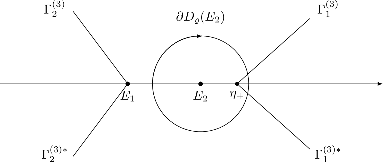
\(M^{(err)}(k)\) is holomorphic for \(k\in\mathbb{C}\setminus\Gamma^{(err)}\), where \[\Gamma^{(err)}:=\partial D_{\varrho}\left(E_2\right)\cup \Gamma^{(3)};\] see Figure 6 for an illustration.
\(M^{(err)}(k)\) has continuous boundary values \(M^{(err)}_\pm(k)\) on \(k\in \Gamma^{(err)}\) with the jump condition \[M^{(err)}_{+}(k)=M^{(err)}_{-}(k)V^{(err)}(k),\] where \[\begin{align} \label{equ:jump32Verr32RII} V^{(err)}(k)= \begin{cases} M^{(\infty)}_-(k)V^{(3)}(k){M^{(\infty)}_+(k)}^{-1}, & k\in\Gamma^{(3)}\setminus \overline{D_\varrho(E_2)},\\ \widetilde{M}^{(loc)}(k){M^{(\infty)}(k)}^{-1}, & k\in\partial D_\varrho(E_2),\\ \widetilde{M}^{(loc)}_-(k)V^{(3)}(k){\widetilde{M}^{(loc)}_+(k)}^{-1}, & k\in\Gamma^{(3)}\cap D_\varrho(E_2). \end{cases} \end{align}\qquad{(17)}\]
As \(k\rightarrow\infty\) in \(k\in\mathbb{C}\setminus\Gamma^{(err)}\), we have \(M^{(err)}(k)=I+\mathcal{O}(k^{-1})\).
As \(k\rightarrow E_1\), we have \(M^{(err)}(k)=\mathcal{O}(1)\).
Using item (c) in Proposition 7, item (c) in Proposition 8, Proposition 9 and Lemma 2, a straightforward calculation yields the following proposition.
Proposition 10. For \(\xi\in\mathcal{T}_\mathrm{\uppercase{\romannumeral1}}\), the function \(V^{(err)}(\cdot)-I:\Gamma^{(err)}\to\mathbb{C}^{2\times2}\) lies in \(L^p\left(\Gamma^{(err)}\right)\) for \(p=1,2,\infty\), and uniformly for \(\xi\in\mathcal{T}_\mathrm{\uppercase{\romannumeral1}}\), it holds that \[\begin{align} &\Vert V^{(err)}(k)-I \Vert_{L^p\left(\Gamma^{(err)}\setminus\overline{D_\varrho(E_2)}\right)}= \mathcal{O}(\mathrm{e}^{-ct}), \label{Ve-I-1}\\ &\Vert V^{(err)}(k)-I \Vert_{L^p\left(\partial D_\varrho(E_2)\right)}=\mathcal{O}(t^{\gamma_p}),\label{Ve-I-2}\\ &\Vert V^{(err)}(k)-I \Vert_{L^p\left(\mathbb{R}\setminus\left(\overline{D_\varrho(E_2)}\right)\right)}=\mathcal{O}(t^{-1}),\label{Ve-I-3}\\ &\Vert V^{(err)}(k)-I \Vert_{L^p\left(\Gamma^{(err)}\cap D_\varrho(E_2)\right)}=\mathcal{O}(t^{\omega_p}).\label{Ve-I-4} \end{align}\] {#eq: sublabel=eq:Ve-I-1,eq:Ve-I-2,eq:Ve-I-3,eq:Ve-I-4} where \(c>0\), \[\begin{align} \gamma_1=-\frac{1}{3},\;\gamma_2=-\frac{\epsilon_1}{2},\gamma_\infty=\frac{1}{3}-\epsilon_1;\quad \omega_1=-1,\;\omega_2=-\frac{2}{3},\omega_\infty=-\frac{1}{3}. \end{align}\] In particular, uniformly for \(\xi\in\mathcal{T}_\mathrm{\uppercase{\romannumeral1}}\), it holds that \[\label{equ:unifrom32V-I} \Vert V^{(err)}(k)-I \Vert_{L^p\left(\Gamma^{(err)}\right)}=\mathcal{O}(t^{\gamma_p}), \quad p=1,2,\infty.\qquad{(18)}\]
Proof. According to the definition of \(V^{(err)}\) in ?? We have \[V^{(err)}-I =\begin{cases} M^{(\infty)}\left(V^{(3)}-I\right){M^{(\infty)}}^{-1}, & k\in\Gamma^{(3)}\setminus \left(\overline{D_\varrho(E_2)}\cup[E_1,E_2]\right),\\ M^{(\infty)}_-\left(V^{(3)}-V^{(\infty)}\right){M^{(\infty)}_+}^{-1}, & k\in[E_1,E_2]\setminus \overline{D_\varrho(E_2)},\\ \widetilde{M}^{(loc)}{M^{(\infty)}}^{-1}-I, & k\in\partial D_\varrho(E_2),\\ \widetilde{M}^{(loc)}_-\left(V^{(3)}-\widetilde{V}^{(loc)}\right){\left(\widetilde{M}^{(loc)}_{+}\right)}^{-1}, & k\in\Gamma^{(3)}\cap D_\varrho(E_2). \end{cases}\] Due to the signature of \(g_\mathrm{\uppercase{\romannumeral1}}\) outside \(\overline{D_\varrho(E_2)}\cup\mathbb{R}\), we infer from item (b) of Proposition 7 that \(\Vert V^{(err)}(k)-I \Vert_{L^p\left(\Gamma^{(err)}\setminus\left(\overline{D_\varrho(E_2)}\cup\mathbb{R}\right)\right)}\) has exponential decay as \(t\to+\infty\). Moreover, item (c) of Proposition 7 implies that \(\Vert V^{(err)}(k)-I \Vert_{L^p\left(\mathbb{R}\setminus\overline{D_\varrho(E_2)}\right)}=\mathcal{O}(t^{-1})\) uniformly for \(\xi\in\mathcal{T}_\mathrm{\uppercase{\romannumeral1}},\;p=1,2,\infty.\) It can be inferred from Lemma 2 that ?? and ?? hold respectively. ◻
It then follows from the small norm RH problem theory [52] that there exists a unique solution to RH problem 10 for large positive \(t\). Furthermore, according to Beals-Coifman theory [53], the solution to \(M^{(err)}\) can be given by \[\label{equ:BCsolforError} M^{(err)}(k) = I + \frac{1}{2\pi \mathrm{i}} \int_{\Gamma^{(err)}} \frac{(I + \varpi(z))(V^{(err)}(z) - I)}{z - k} \mathop{}\!\mathrm{d}z,\tag{53}\] where \(\varpi \in L^2(\Gamma^{(err)})\) is the unique solution of \((1 - C_{V^{(err)}})\varpi = C_{V^{(err)}} I\). And \(C_{V^{(err)}}: L^2(\Gamma^{(err)}) \to L^2(\Gamma^{(err)})\) is the Cauchy operator on \(\Gamma^{(err)}\), which is defined as \(C_{V^{(err)}}(f)(k) = C_{-}f(V^{(err)} - I)\) with \(C_{-}\) being the Cauchy projection operator on \(\Gamma^{(err)}\). The existence and uniqueness of \(\varpi\) come from the boundedness of the Cauchy operator \(C_{-}\), which admits \[\begin{align} \label{CverrL2} \|C_{V^{(err)}}\|_{L^2(\Gamma^{(err)})} \leqslant \|C_{-}\|_{L^2(\Gamma^{(err)}) \to L^2(\Gamma^{(err)})} \|V^{(err)} - I\|_{L^\infty(\Gamma^{(err)})} = \mathcal{O}(t^{1/3-\epsilon_1}). \end{align}\tag{54}\] In addition, \[\label{equ:estiforvarpi} \|\varpi\|_{L^2(\Gamma^{(err)})} \leqslant \frac{\|C_{V^{(err)}}\|_{L^2(\Gamma^{(err)})}}{1 - \|C_{V^{(err)}}\|_{L^2(\Gamma^{(err)})}} \lesssim t^{1/3-\epsilon_1}.\tag{55}\]
Moreover, by 53 , it follows that \[M^{(err)}(k)=I+\frac{M^{(err)}_1}{k}+\mathcal{O}(k^{-2}), \quad k\rightarrow\infty,\] where \[\label{equ:Merr95132TI} M^{(err)}_1=-\frac{1}{2\pi \mathrm{i}}\int_{\Gamma^{(err)}}\left(I + \varpi(z)\right)(V^{(err)}(z)-I)\mathop{}\!\mathrm{d}z.\tag{56}\] Therefore, we obtain the following proposition.
Proposition 11. For \(\xi\in\mathcal{T}_\mathrm{\uppercase{\romannumeral1}}\), as \(t\rightarrow+\infty\), we have \[\label{equ:Merr95132RII} \begin{align} M^{(err)}_1&=-\frac{1}{8}\left(\frac{3}{2}\right)^{-\frac{1}{3}}(2\alpha)^{\frac{1}{2}}\left|g_{\mathrm{\uppercase{\romannumeral1}}}^{(2)}(E_2)\right|^{-\frac{1}{3}}s^2t^{-\frac{1}{3}}\begin{pmatrix}\mathrm{i}&1\\1&-\mathrm{i}\end{pmatrix}+\mathcal{O}(t^{\frac{2}{3}-2\epsilon_1}), \end{align}\qquad{(19)}\] where \(g_{\mathrm{\uppercase{\romannumeral1}}}^{(2)}(E_2)\) and \(s\) are given by 34 and 39 respectively.
Proof. We first divide \(M^{(err)}_1\) into four parts by \[\begin{align} &I_1:=-\frac{1}{2\pi \mathrm{i}}\int_{\Gamma^{(err)}}\varpi(z)\left(V^{(err)}(z)-I\right)\mathop{}\!\mathrm{d}z, \\ &I_2:=-\frac{1}{2\pi \mathrm{i}}\int_{\Gamma^{(err)}\setminus D_\varrho(E_2)}\left(V^{(err)}(z)-I\right)\mathop{}\!\mathrm{d}z, \\ &I_3:=-\frac{1}{2\pi \mathrm{i}}\oint_{\partial D_\varrho(E_2)}\left(V^{(err)}(z)-I\right)\mathop{}\!\mathrm{d}z,\\ &I_4:=-\frac{1}{2\pi \mathrm{i}}\int_{\Gamma^{(err)}\cap D_\varrho(E_2)}\left(V^{(err)}(z)-I\right)\mathop{}\!\mathrm{d}z. \end{align}\] The main contribution to \(M^{(err)}_1\) stems from the \(I_3\). For the other three parts, we have the following estimates: \(I_1=\mathcal{O}(t^{2/3-2\epsilon_1})\) by 55 and ?? , \(I_2=\mathcal{O}(\mathrm{e}^{-ct})\) by ?? , and \(I_4=\mathcal{O}(t^{-1})\) by ?? .
Now we turn to estimate \(I_3\). From Lemma 2 and ?? , we have \[\begin{align} I_3=&-\frac{1}{2\pi \mathrm{i}}\oint_{\partial D_\varrho(E_2)}\left(V^{(err)}(z)-I\right)\mathop{}\!\mathrm{d}z\\ =&-\frac{1}{2\pi \mathrm{i}}\oint_{\partial D_\varrho(E_2)}P(z;\xi,t)\left(\frac{M_1^{P_{34}}(s)}{\zeta(z)}+\mathcal{O}(\zeta^{-2}) \right) P(z;\xi,t)^{-1}\mathop{}\!\mathrm{d}z\\ =&-\frac{1}{2\pi \mathrm{i}}\oint_{\partial D_\varrho(E_2)}\frac{t^{1/3}}{\zeta(z)}P(z;\xi,1)\begin{pmatrix} 0&\left(M_1^{P_{34}}(s)\right)_{12}\\0&0 \end{pmatrix} P(z;\xi,1)^{-1}\mathop{}\!\mathrm{d}z+\mathcal{O}(t^{-\frac{2}{3}})\\ =&-\frac{(\frac{3}{2})^{-2/3}\left|g_{\mathrm{\uppercase{\romannumeral1}}}^{(2)}(E_2)\right|^{-2/3}}{t^{1/3}}P(E_2;\xi,1)\begin{pmatrix} 0&\left(M_1^{P_{34}}(s)\right)_{12}\\0&0 \end{pmatrix} P(E_2;\xi,1)^{-1}+\mathcal{O}(t^{-\frac{2}{3}}), \end{align}\] where we have uses the residue theorem in the last equality. Taking into the results of \(P(E_2;\xi,1)\) and \(\left(M_1^{P_{34}}(s)\right)_{12}\) in 51 and 104 respectively, we obtain \[\label{equ:I95332TI} I_3=-\frac{1}{8}\left(\frac{3}{2}\right)^{-\frac{1}{3}}(2\alpha)^{\frac{1}{2}}\left|g_{\mathrm{\uppercase{\romannumeral1}}}^{(2)}(E_2)\right|^{-\frac{1}{3}}s^2t^{-\frac{1}{3}}\begin{pmatrix}\mathrm{i}&1\\1&-\mathrm{i}\end{pmatrix}+\mathcal{O}(t^{-\frac{2}{3}}).\tag{57}\] Based on the analysis above, we obtain the desired result given in ?? . ◻
3.6 Proof of the part () of Theorem 1↩︎
By tracing back the transformations 28 , 30 , 31 and 52 , we conclude, for \(k\in\mathbb{C}\setminus\left(\Gamma^{(3)}\cap D_\varrho(E_2)\right)\), \[M(k)=\mathrm{e}^{\mathrm{i}tg_{\mathrm{\uppercase{\romannumeral1}},\infty}(\xi)\sigma_3}D_{\mathrm{\uppercase{\romannumeral1}},\infty}(\xi)^{-\sigma_3}M^{(err)}(k)M^{(\infty)}(k)D_{\mathrm{\uppercase{\romannumeral1}}}^{\sigma_3}(k)G^{-1}(k)\mathrm{e}^{-\mathrm{i}t(g_{\mathrm{\uppercase{\romannumeral1}}}(k)-\theta(k))\sigma_3},\] where \(g_{\mathrm{\uppercase{\romannumeral1}}}\), \(D_{\mathrm{\uppercase{\romannumeral1}}}\), \(M^{(err)}\), \(M^{(\infty)}\) and \(G\) are defined in 26 , 29 , 52 , ?? and 32 respectively. From the reconstruction formula stated in 24 , we obtain that \[u(x,t)=2\mathrm{i}\mathrm{e}^{2\mathrm{i}tg_{\mathrm{\uppercase{\romannumeral1}},\infty}(\xi)} D_{\mathrm{\uppercase{\romannumeral1}},\infty}^{-2}(\xi)\left[(M^{(err)}_1)_{12}+\lim_{k\rightarrow\infty}k\left(M^{(\infty)}(k)\right)_{12}\right].\] It now follows from item (a) of Lemma [lemma:minfty32for32T1] and Proposition 11 that part () of Theorem 1 holds.
4 Asymptotic analysis of the RH problem for \(M\) in \(\mathcal{T}_{\mathrm{\uppercase{\romannumeral2}}}\)↩︎
This section is devoted to the long-time asymptotic analysis of the RH problem 1 in the region \(\mathcal{T}_{\mathrm{\uppercase{\romannumeral2}}}\).
4.1 First transformation: \(M\rightarrow M^{(1)}\)↩︎
We begin with the introduction of the \(g\)-function [46], [50], [51]. For \(\xi\in\mathcal{T}_{\mathrm{\uppercase{\romannumeral2}}}\), we introduce \[\label{equ:g32function32TII} g_{\mathrm{\uppercase{\romannumeral2}}}(k)=g_{\mathrm{\uppercase{\romannumeral2}}}(k;\xi):=2(k-k_0)\mathcal{X}(k), \quad \mathcal{X}(k)=\mathcal{X}(k;\xi):=\sqrt{(k-E_1)(k-k_0)},\tag{58}\] where the branch of the square root being chosen such that \(\mathcal{X}(k)=k+\mathcal{O}(k^{-1})\) as \(k\rightarrow\infty\) with \(k_0=k_0(\xi):=-\frac{E_1+\xi}{3}\). It is readily verified that \(g_{\mathrm{\uppercase{\romannumeral2}}}\) has the following properties.
Proposition 12. The function \(g_{\mathrm{\uppercase{\romannumeral2}}}\) defined in 58 satisfies the following properties:
\(g_{\mathrm{\uppercase{\romannumeral2}}}(k)\) is holomorphic for \(k\in\mathbb{C}\setminus[E_1,k_0]\).
As \(k\rightarrow\infty\) in \(\mathbb{C}\setminus[E_1,k_0]\), we have \(g_{\mathrm{\uppercase{\romannumeral2}}}(k)=\theta(k)+g_{\mathrm{\uppercase{\romannumeral2}},\infty}(\xi)+\mathcal{O}(k^{-1})\), where \[g_{\mathrm{\uppercase{\romannumeral2}},\infty}(\xi)=\frac{\xi^2-4E_1\xi-8E_1^2}{12}.\]
For \(k\in(E_1,k_0)\), \(g_{\mathrm{\uppercase{\romannumeral2}},+}(k)+g_{\mathrm{\uppercase{\romannumeral2}}, -}(k)=0\).
For \(k\in\mathbb{C}\setminus [E_1,k_0]\), \(g(k)\) obeys the symmetry \(g_{\mathrm{\uppercase{\romannumeral2}}}(k)=g_{\mathrm{\uppercase{\romannumeral2}}}^*(k)\).
As \(k\to E_1\), we have \[\label{g95II32asy32E951} g_{\mathrm{\uppercase{\romannumeral2}}}(k)=-2(k_0-E_1)^{\frac{3}{2}}(E_1-k)^{\frac{1}{2}}-3(k_0-E_1)^{\frac{1}{2}}(E_1-k)^{\frac{3}{2}}+\mathcal{O}((E_1-k)^{\frac{5}{2}}).\qquad{(20)}\]
It is readily seen that the \(k\)-derivative of \(g_{\mathrm{\uppercase{\romannumeral2}}}\) is given by \[\label{g95239} g_{\mathrm{\uppercase{\romannumeral2}}}'(k)=\frac{4\left(k-\eta_-(\xi)\right)\left(k-\eta_+(\xi)\right)}{\mathcal{X}(k)},\tag{59}\] where \[\begin{align} \eta_+(\xi)=k_0,\quad \eta_-(\xi)=\frac{8E_1-\xi}{12}\in(E_1,k_0). \end{align}\] In the transition region \(\mathcal{T}_{\mathrm{\uppercase{\romannumeral2}}}\), saddle point \(k_0\) tends to \(E_1\) with at least the speed of \(\mathcal{O}(t^{-\frac{2}{3}})\) as \(t\to+\infty\). The signature table for \(\mathop{\mathrm{Im}}g_{\mathrm{\uppercase{\romannumeral2}}}\) is illustrated in Figure 7.
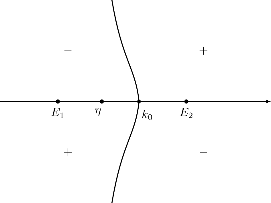
4.1.1 RH problem for \(M^{(1)}\)↩︎
By the function \(g_{\mathrm{\uppercase{\romannumeral2}}}\) defined in 58 , we introduce a new matrix-valued function \(M^{(1)}\) by \[\label{def:M132RII} M^{(1)}(k)= M^{(1)}(k;x,t):=\mathrm{e}^{-\mathrm{i}tg_{\mathrm{\uppercase{\romannumeral2}},\infty}(\xi)\sigma_3}M(k)\mathrm{e}^{\mathrm{i}t\left(g_{\mathrm{\uppercase{\romannumeral2}}}(k)-\theta(k)\right)\sigma_3}.\tag{60}\] Then the RH problem for \(M^{(1)}\) reads as follows:
RH problem 11.
\(M^{(1)}(k)\) is holomorphic for \(k\in\mathbb{C}\setminus\mathbb{R}\).
\(M^{(1)}(k)\) has continuous boundary values \(M_{\pm}^{(1)}(k)\) on \(\mathbb{R}\) with the jump condition \[M^{(1)}_{+}(k)=M^{(1)}_{-}(k)V^{(1)}(k), \quad k\in\mathbb{R},\] where \[\label{equ:jump32V132RII} V^{(1)}(k)= \begin{cases} \begin{pmatrix}1-r(k)r^*(k) & r^*(k)\mathrm{e}^{-2\mathrm{i}tg_{\mathrm{\uppercase{\romannumeral2}}}(k)}\\ -r(k)\mathrm{e}^{2\mathrm{i}tg_{\mathrm{\uppercase{\romannumeral2}}}(k)} & 1\end{pmatrix}, &k\in\mathbb{R}\setminus[E_1,k_0], \\ \begin{pmatrix}0 & r^*(k)\\- r(k) & \mathrm{e}^{-2\mathrm{i}tg_{\mathrm{\uppercase{\romannumeral2}},+}(k)} \end{pmatrix}, &k\in[E_1,k_0]. \end{cases}\qquad{(21)}\]
As \(k\rightarrow\infty\) in \(\mathbb{C}\setminus\mathbb{R}\), we have \(M^{(1)}(k)=I+\mathcal{O}(k^{-1})\).
4.2 Second transformation: \(M^{(1)}\rightarrow M^{(2)}\)↩︎
In this section, we introduce an auxiliary function \(D_{\mathrm{\uppercase{\romannumeral2}}}\) to pave the way for the subsequent contour deformation along the ray \((-\infty, E_1)\). Moreover, we need to keep the segments \([E_2,k_0]\) on the line.
4.2.1 The \(D_{\mathrm{\uppercase{\romannumeral2}}}\) function↩︎
Define \(D_{\mathrm{\uppercase{\romannumeral2}}}: \mathbb{C}\setminus\left((-\infty,E_1]\cup[E_1,k_0]\right) \times \mathcal{T}_{\mathrm{\uppercase{\romannumeral2}}}\to\mathbb{C}\) by \[\label{equ:def32D32function32RII} \begin{align} D_{\mathrm{\uppercase{\romannumeral2}}}(k)=D_{\mathrm{\uppercase{\romannumeral2}}}(k;\xi):=\exp\left[\frac{\mathcal{X}(k)}{2\pi \mathrm{i}} \left(\int_{-\infty}^{E_1}\frac{\log \left(1-r(p)r^*(p)\right)}{\mathcal{X}(p)(p-k)}\mathop{}\!\mathrm{d}p+\int_{E_1}^{k_0} \frac{\log r(p)}{\mathcal{X}_{+}(p)(p-k)}\mathop{}\!\mathrm{d}p\right)\right], \end{align}\tag{61}\] where the branch of the function \(\log r(p)\) is such that it is continuous for \(p\in[E_1,k_0]\) and the principal branch is used for \(\log r(E_1)\). The necessary properties of the function \(D_{\mathrm{\uppercase{\romannumeral2}}}\) are given as follows.
Proposition 13. The function \(D_{\mathrm{\uppercase{\romannumeral2}}}\) defined in 61 satisfies the following properties for \(\xi\in \mathcal{T}_{\mathrm{\uppercase{\romannumeral2}}}\):
\(D_{\mathrm{\uppercase{\romannumeral2}}}(k)\) is holomorphic for \(k\in \mathbb{C}\setminus((-\infty,E_1]\cup[E_1,k_0])\).
\(D_{\mathrm{\uppercase{\romannumeral2}}}(k)\) satisfies the following jump relations: \[\begin{align} & D_{\mathrm{\uppercase{\romannumeral2}}, +}(k)=D_{\mathrm{\uppercase{\romannumeral2}}, -}(k)\left(1-r(k)r^*(k)\right), &&k\in (-\infty,E_1),\\ & D_{\mathrm{\uppercase{\romannumeral2}}, +}(k)D_{\mathrm{\uppercase{\romannumeral2}}, -}(k)=r(k), &&k\in (E_1,k_0). \end{align}\]
\(D_{\mathrm{\uppercase{\romannumeral2}}}(k)\) admits the symmetry: \(D_{\mathrm{\uppercase{\romannumeral2}}}(k)D^*_{\mathrm{\uppercase{\romannumeral2}}}(k)=1\) for \(k\in\mathbb{C}\setminus(-\infty,E_1)\). In particular, \(D_{\mathrm{\uppercase{\romannumeral2}},+}(k)\overline{D_{\mathrm{\uppercase{\romannumeral2}},-}(k)}=1\) for \(k\in(-\infty,k_0)\setminus\{E_1\}\).
As \(k\rightarrow \infty\), \[D^{\pm 1}_{\mathrm{\uppercase{\romannumeral2}}}(k)=D^{\pm 1}_{\mathrm{\uppercase{\romannumeral2}},\infty}(\xi)+\mathcal{O}(k^{-1})\] uniformly for all \(\xi\in\mathcal{T}_{\mathrm{\uppercase{\romannumeral2}}}\), where \[D_{\mathrm{\uppercase{\romannumeral2}},\infty}(\xi)=\exp\left[-\frac{1}{2\pi \mathrm{i}} \left(\int_{-\infty}^{E_1}\frac{\log \left(1-r(p)r^*(p)\right)}{\mathcal{X}(p)}\mathop{}\!\mathrm{d}p+\int_{E_1}^{k_0} \frac{\log r(p)}{\mathcal{X}_{+}(p)}\mathop{}\!\mathrm{d}p\right)\right]\] with \(| D_{\mathrm{\uppercase{\romannumeral2}},\infty}(\xi)|=1\) for all \(\xi\in\mathcal{T}_{\mathrm{\uppercase{\romannumeral2}}}\).
At the branch point \(E_1\), we have: \[D_{\mathrm{\uppercase{\romannumeral2}}}(k)=(k-E_1)^{1/4}\mathrm{e}^{d_{0}}\left[1+\mathcal{O}\left((k-E_1)^{1/2}\right)\right], \quad k\to E_1\in\overline{\mathbb{C^+}}\] uniformly for \(\xi\in\mathcal{T}_{\mathrm{\uppercase{\romannumeral2}}}\), where \[\label{equ:def32of32d0} d_{0}=\frac{1}{2} \log \left(\overline{q_{1,0}} q_{1,1}+q_{1,0} \overline{q_{1,1}}\right)+\frac{1}{2} \log q_{1,0} \in \mathbb{C}\qquad{(22)}\] and the principal branch is used for the fourth root and the logarithms. By symmetry, a similar formula holds for \(k \rightarrow E_1\in\overline{\mathbb{C}^{-}}\).
As \(k\in\mathbb{C}\setminus(-\infty,k_0)\) approaches \(k_0\), \(D_{\mathrm{\uppercase{\romannumeral2}}}(k)\) has the following asymptotics \[\begin{align} &D_{\mathrm{\uppercase{\romannumeral2}}}(k)=\sqrt{r(k_0)}+\mathcal{O}\left((k-k_0)^{1/2}\right),&& k\to k_0,\\ & D_{\mathrm{\uppercase{\romannumeral2}}}^{-1}(k)=\frac{1}{\sqrt{r(k_0)}}+\mathcal{O}\left((k-k_0)^{1/2}\right),&& k\to k_0, \end{align}\] uniformly for \(\xi\in\mathcal{T}_{\mathrm{\uppercase{\romannumeral2}}}\).
Proof. This proposition is the same with [48], whose proof is omitted here. ◻
4.2.2 RH problem for \(M^{(2)}\)↩︎
With the help of \(D_{\mathrm{\uppercase{\romannumeral2}}}\) function, we define \[\label{def:M232RII} M^{(2)}(k)= M^{(2)}(k;x,t):= D_{\mathrm{\uppercase{\romannumeral2}},\infty}(\xi)^{\sigma_3}M^{(1)}(k)D_{\mathrm{\uppercase{\romannumeral2}}}^{-\sigma_3}(k).\tag{62}\] Then RH problem for \(M^{(2)}\) reads as follows:
RH problem 12.
\(M^{(2)}(k)\) is holomorphic for \(k\in\mathbb{C}\setminus\mathbb{R}\).
\(M^{(2)}(k)\) has continuous boundary values \(M_{\pm}^{(2)}(k)\) on \(\mathbb{R}\) with the jump condition \[M^{(2)}_{+}(k)=M^{(2)}_{-}(k)V^{(2)}(k),\] where \[V^{(2)}(k)= \begin{cases} \begin{pmatrix} 1&D_{\mathrm{\uppercase{\romannumeral2}},+}^2(k)r_2(k)\mathrm{e}^{-2\mathrm{i}tg_\mathrm{\uppercase{\romannumeral2}}(k)}\\-D_{\mathrm{\uppercase{\romannumeral2}},-}^{-2}(k)r^*_2(k)\mathrm{e}^{2\mathrm{i}tg_\mathrm{\uppercase{\romannumeral2}}(k)}&1-r(k)r^*(k) \end{pmatrix},&k\in(-\infty,E_1),\\ \begin{pmatrix}0 & 1\\ -1 & D_{\mathrm{ \uppercase{\romannumeral2}}, +}(k)D_{\mathrm{\uppercase{\romannumeral2}}, -}^{-1}(k)\mathrm{e}^{-2\mathrm{i}tg_{\mathrm{\uppercase{\romannumeral2}},+}(k)} \end{pmatrix}, &k\in (E_1,k_0),\\ \begin{pmatrix}1-r(k)r^*(k) & D_{\mathrm{\uppercase{\romannumeral2}}}^2(k)r^*(k)\mathrm{e}^{-2\mathrm{i}tg_\mathrm{\uppercase{\romannumeral2}}(k)}\\ -D_{\mathrm{\uppercase{\romannumeral2}}}^{-2}(k)r(k)\mathrm{e}^{2\mathrm{i}tg_\mathrm{\uppercase{\romannumeral2}}(k)} & 1\end{pmatrix}, &k\in(k_0,+\infty). \end{cases}\]
As \(k\rightarrow\infty\) in \(\mathbb{C}\setminus\mathbb{R}\), we have \(M^{(2)}(k)=I+\mathcal{O}(k^{-1})\).
4.3 Third transformation: \(M^{(2)}\rightarrow M^{(3)}\)↩︎
The aim of the third transformation is to open lenses in regions \(U^{(3)}_j,U^{(3)*}_j,\;j=1,2\), which are illustrated in Figure 8. Following the same operations given by Proposition 7 and Proposition 8, we can obtain the analytic approximation for the spectral function \(r\) in region \(U^{(3)}_1\) (denoted as \(r_a\)), as well as the analytic approximation for \(r_2\) in region \(U^{(3)}_2\) (denoted as \(r_{2,a}\)).

Now we are ready to introduce a transformation \[\label{def:M332RII} M^{(3)}(k)=M^{(3)}(k;x,t):=M^{(2)}(k)D_{\mathrm{\uppercase{\romannumeral2}}}^{\sigma_3}(k)G(k)D_{\mathrm{\uppercase{\romannumeral2}}}^{-\sigma_3}(k),\tag{63}\] where \[\label{def:G40k4132T2} G(k):= \begin{cases} \begin{pmatrix}1 & 0 \\ r_a\mathrm{e}^{2\mathrm{i}tg_{\mathrm{\uppercase{\romannumeral1}}}} & 1\end{pmatrix}, &k\in U^{(3)}_1, \\ \begin{pmatrix}1 & r_a^{*}\mathrm{e}^{-2\mathrm{i}tg_\mathrm{\uppercase{\romannumeral1}}} \\ 0 & 1\end{pmatrix}, &k\in U_1^{(3)*}, \\ \begin{pmatrix}1 & -r_{2,a}\mathrm{e}^{-2\mathrm{i}tg_\mathrm{\uppercase{\romannumeral1}}} \\ 0 & 1\end{pmatrix}, &k\in U_2^{(3)},\\ \begin{pmatrix}1 & 0 \\ -r^*_{2,a}\mathrm{e}^{2\mathrm{i}tg_\mathrm{\uppercase{\romannumeral1}}} & 1\end{pmatrix}, & k\in U_2^{(3)*},\\ I, &\textrm{elsewhere}. \end{cases}\tag{64}\] Here, the domains \(U^{(3)}_j\) for \(j=1,2\) are illustrated in Figure 8.
Then RH problem for \(M^{(3)}\) reads as follows:
RH problem 13.
\(M^{(3)}(k)\) is holomorphic for \(k\in\mathbb{C}\backslash\Gamma^{(3)}\), where \(\Gamma^{(3)}:=\cup_{j=1}^{2}(\Gamma^{(3)}_j\cup\Gamma_j^{(3)*})\cup\mathbb{R}\); see Figure 3 for an illustration.
\(M^{(3)}(k)\) has continuous boundary values \(M_{\pm}^{(3)}(k)\) on \(k\in \Gamma^{(3)}\) with the jump condition \[M^{(3)}_{+}(k)= M^{(3)}_{-}(k)V^{(3)}(k),\] where \[\label{equ:jump32V332RII} V^{(3)}(k)= \begin{cases} \begin{pmatrix} 1 & 0\\ -D_{\mathrm{\uppercase{\romannumeral2}}}^{-2}(k)r_a(k)\mathrm{e}^{2\mathrm{i}tg_\mathrm{\uppercase{\romannumeral2}}(k)} & 1\end{pmatrix}, &k\in\Gamma^{(3)}_1, \\ \begin{pmatrix} 1 & D_{\mathrm{\uppercase{\romannumeral2}},+}^{2}(k)r_{2,a}(k)\mathrm{e}^{-2\mathrm{i}tg_\mathrm{\uppercase{\romannumeral2}}(k)}\\ 0& 1\end{pmatrix}, &k\in\Gamma^{(3)}_2, \\ \begin{pmatrix} 1 & D_{\mathrm{\uppercase{\romannumeral2}}}^{2}(k)r_a^*(k)\mathrm{e}^{-2\mathrm{i}tg_\mathrm{\uppercase{\romannumeral2}}(k)}\\ 0 & 1\end{pmatrix}, & k\in\Gamma^{(3)*}_1, \\ \begin{pmatrix} 1 & 0\\ -D_{\mathrm{\uppercase{\romannumeral2}},-}^{-2}(k)r_{2,a}^*(k)\mathrm{e}^{2\mathrm{i}tg_\mathrm{\uppercase{\romannumeral2}}(k)} & 1\end{pmatrix}, & k\in\Gamma^{(3)*}_2, \\ \begin{pmatrix} 1-r_r(k)r^*_r(k)&D_\mathrm{\uppercase{\romannumeral2}}^2(k)r_r^*(k)\mathrm{e}^{-2\mathrm{i}tg_\mathrm{\uppercase{\romannumeral2}}(k)}\\-D_\mathrm{\uppercase{\romannumeral2}}^{-2}(k)r_r(k)\mathrm{e}^{2\mathrm{i}tg_\mathrm{\uppercase{\romannumeral2}}(k)}&1 \end{pmatrix},&k\in(k_0,+\infty),\\ \begin{pmatrix} 1&D_\mathrm{\uppercase{\romannumeral2},+}^2(k)r_{2,r}(k)\mathrm{e}^{-2\mathrm{i}tg_\mathrm{\uppercase{\romannumeral2}}(k)}\\-D_{\mathrm{\uppercase{\romannumeral2}},-}^{-2}(k)r^*_{2,r}(k)\mathrm{e}^{2\mathrm{i}tg_\mathrm{\uppercase{\romannumeral2}}(k)}&1-r_r(k)r^*_r(k) \end{pmatrix},&k\in(-\infty,E_1),\\ \begin{pmatrix} 0&1\\-1&D_{\mathrm{\uppercase{\romannumeral2}},+}(k)D_{\mathrm{\uppercase{\romannumeral2}},-}^{-1}(k)\mathrm{e}^{-2\mathrm{i}tg_{\mathrm{\uppercase{\romannumeral2}},+}(k)}\\ \end{pmatrix},&k\in(E_1,k_0). \end{cases}\qquad{(23)}\]
As \(k\rightarrow\infty\) in \(\mathbb{C}\setminus\Gamma^{(3)}\), we have \(M^{(3)}(k)=I+\mathcal{O}(k^{-1})\).
4.4 Analysis of RH problem for \(M^{(3)}\)↩︎
It is readily seen that \(V^{(3)} \to I\) exponentially on the contours \(\Gamma^{(3)}_j \cup \Gamma_j^{(3)*}\) for \(j=1,2\) as \(t \to +\infty\) except around the point \(E_1\) and \(k_0\) which leads us to consider the following global parametrix.
4.4.1 Global parametrix↩︎
For \(\xi \in \mathcal{T}_\mathrm{\uppercase{\romannumeral2}}\), the global parametrix \(M^{(\infty)}(k)\) satisfies the following RH problem.
RH problem 14.
\(M^{(\infty)}(k)\) is holomorphic for \(k\in\mathbb{C}\setminus[E_1,k_0]\).
\(M^{(\infty)}(k)\) has continuous boundary values \(M_{\pm}^{(\infty)}(k)\) on \((E_1,k_0)\) satisfying the following jump condition: \[\begin{align} M_{+}^{(\infty)}(k)=M_{-}^{(\infty)}(k)V^{(\infty)}(k), \end{align}\] where \[V^{(\infty)}(k)=\begin{pmatrix} 0 & 1\\ -1 & 0 \end{pmatrix}.\]
As \(k\rightarrow\infty\) in \(\mathbb{C}\setminus[E_1,k_0]\), we have \(M^{(\infty)}(k)=I+\mathcal{O}(k^{-1})\).
Lemma 3. The RH problem 14 has a unique solution which is given by \[\label{equ:sol32of32Minfty32for32TII} M^{(\infty)}(k)=\frac{1}{2} \left( \begin{array}{cc} \kappa(k)+\kappa^{-1}(k) & -\mathrm{i}\left(\kappa(k)-\kappa^{-1}(k)\right)\\ \mathrm{i}\left(\kappa(k)-\kappa^{-1}(k)\right) & \kappa(k)+\kappa^{-1}(k) \end{array} \right),\qquad{(24)}\] where \(\kappa\) is defined by \[\kappa(k)=\kappa(k;\xi):=\left(\frac{k-k_0}{k-E_1}\right)^{\frac{1}{4}}\] with the branch is chosen such that \(\kappa(k)=1+\mathcal{O}(k^{-1})\) as \(k\to\infty\). Moreover, for \(\xi \in \mathcal{T}_\mathrm{\uppercase{\romannumeral2}}\), the following expansions hold true for \(M^{(\infty)}\):
As \(k\rightarrow\infty\) in \(\mathbb{C}\setminus[E_1,k_0]\), \[M^{(\infty)}(k)=I+\frac{\mathrm{i}(k_0-E_1)}{4k}\begin{pmatrix} 0&1\\-1&0 \end{pmatrix}+\mathcal{O}(k^{-2}).\]
As \(k\rightarrow E_1\), \[\begin{align} M^{(\infty)}(k)&= \frac{\left(k_0-E_1\right)^{1 / 4}}{2\left(E_1-k\right)^{1 / 4}}\left\{\begin{pmatrix} 1 & -\mathrm{i}\\ \mathrm{i}& 1 \end{pmatrix}+\frac{\left(E_1-k\right)^{1 / 2}}{\left(k_0-E_1\right)^{1 / 2}}\begin{pmatrix} 1 & \mathrm{i}\\ -\mathrm{i}& 1 \end{pmatrix}+\mathcal{O}\left(\left|k-E_1\right|\right)\right\}. \end{align}\]
As \(k\rightarrow k_0\), \[\begin{align} M^{(\infty)}(k)&= \frac{\left(k_0-E_1\right)^{1 / 4}}{2\left(k-k_0\right)^{1 / 4}}\left\{\begin{pmatrix} 1 & \mathrm{i}\\ -\mathrm{i}& 1 \end{pmatrix}+\frac{\left(k-k_0\right)^{1 / 2}}{\left(k_0-E_1\right)^{1 / 2}}\begin{pmatrix} 1 & -\mathrm{i}\\ \mathrm{i}& 1 \end{pmatrix}+\mathcal{O}\left(\left|k-k_0\right|\right)\right\}. \end{align}\]
4.4.2 Local parametrix near \(E_1\) and \(k_0\)↩︎
Let \[\begin{align} \label{def32local32RII} D_\varrho(E_1)=\left\{k: |k-E_1|<\varrho \right\},\quad D_\varrho(k_0)=\left\{k: |k-k_0|<\varrho \right\} \end{align}\tag{65}\] be a small disk around \(E_1\) and \(k_0\), where \(\varrho=\frac{1}{3}(k_0-E_1)\). We intend to solve the following local RH problem \(M^{(loc,y)}\) for \(y\in\{E_1,k_0\}\).
RH problem 15.
\(M^{(loc,y)}(k)\) is holomorphic for \(k\in\overline{D_{\varrho}( y)}\setminus\Gamma^{(loc,y)}\) , where \[\begin{align} \label{def:Gamma9440ell4132RII} \Gamma^{(loc,y)}:=D_\varrho(y)\cap \Gamma^{(3)}; \end{align}\qquad{(25)}\] see Figure 9 for an illustration.
\(M^{(loc,y)}(k)\) has continuous boundary values \(M_{\pm}^{(loc,y)}(k)\) on \(k\in \Gamma^{(loc,y)}\) with the jump condition \[\begin{align} M^{(loc,y)}_{+}(k)=M^{(loc,y)}_{-}(k)V^{(3)}(k)\big|_{\Gamma^{(loc,y)}}, \end{align}\] where \(V^{(3)}(k)\) is given by ?? .
As \(k\rightarrow\infty\) in \(\mathbb{C}\setminus\Gamma^{(loc,y)}\), we have \(M^{(loc,y)}(k)=I+\mathcal{O}(k^{-1})\).
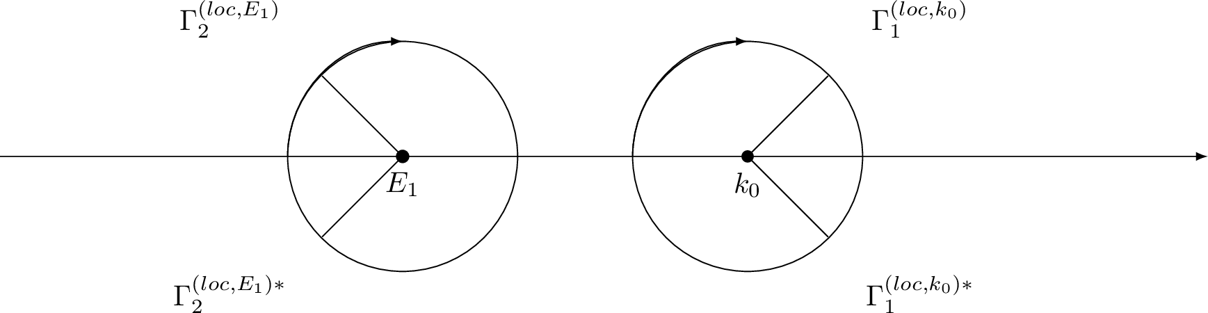
As to the local parametrix near \(E_1\), it can be also be constructed by the Painlevé XXXIV parametrix shown in Appendix 6 in a standard manner. We recall the asymptotics of \(g_{\mathrm{\uppercase{\romannumeral2}}}\) near \(E_1\) that \[g_{\mathrm{\uppercase{\romannumeral2}}}(k)=-2(k_0-E_1)^{\frac{3}{2}}(E_1-k)^{\frac{1}{2}}-3(k_0-E_1)^{\frac{1}{2}}(E_1-k)^{\frac{3}{2}}+\mathcal{O}((E_1-k)^{\frac{5}{2}}).\] By introducing the following rescaling of variable: \[z=(k_0-E_1)^{\frac{1}{3}}(E_1-k),\] we have \[g_{\mathrm{\uppercase{\romannumeral2}}}(z)=g_{\mathrm{\uppercase{\romannumeral2}}}(k(z))=-2(k_0-E_1)^{\frac{4}{3}}z^{\frac{1}{2}}-3z^{\frac{3}{2}}+\mathcal{O}(z^{\frac{5}{2}}),\quad z\to0\in\mathbb{C}\setminus(-\infty,0).\] For \(z \in z\left(D_{\varrho}(E_1)\setminus[E_1,+\infty)\right)\), we set \[\zeta(z) :=-\left(\frac{9}{2}\right)^{\frac{2}{3}}t^{\frac{2}{3}}\left[g_{\mathrm{\uppercase{\romannumeral2}}}(z)+2(k_0-E_1)^{\frac{4}{3}}z^{\frac{1}{2}}\right]^{\frac{2}{3}},\] which implies that \[\label{equ:zeta32TII} \zeta(k)=\zeta(z(k))=-\left(\frac{9}{2}\right)^{\frac{2}{3}}t^{\frac{2}{3}}\left(k_0-E_1\right)^{\frac{1}{3}}(E_1-k)+\mathcal{O}(k-E_1),\quad k\to E_1,\tag{66}\] where the cut \((\cdot)^{\frac{3}{2}}\) runs along \(\mathbb{R}^{-}\). This is a one-to-one conformal mapping form \(k\)-plane to \(\zeta\)-plane as \(\zeta^\prime(E_1)=\left(\frac{9}{2}\right)^{\frac{2}{3}}t^{\frac{2}{3}}\left(k_0-E_1\right)^{\frac{1}{3}}>0\). Moreover, we have \[\label{asy32zeta147232RII} \zeta(k)^{\frac{1}{2}}=\begin{cases} -\mathrm{i}t^{\frac{1}{3}}(\frac{9}{2})^{\frac{1}{3}}(k_0-E_1)^{\frac{1}{6}}(E_1-k)^{\frac{1}{2}}\left(1+\mathcal{O}(k-E_1)\right),&k \to E_1,\;k \in \mathbb{C}^+,\\ \mathrm{i}t^{\frac{1}{3}}(\frac{9}{2})^{\frac{1}{3}}(k_0-E_1)^{\frac{1}{6}}(E_1-k)^{\frac{1}{2}}\left(1+\mathcal{O}(k-E_1)\right),&k \to E_1,\;k \in \mathbb{C}^-, \end{cases}\tag{67}\] as well as \[\label{asy32zeta32347232RII} \zeta(k)^{\frac{3}{2}}=\begin{cases} \frac{9\mathrm{i}}{2}t(k_0-E_1)^{\frac{1}{2}}(E_1-k)^{\frac{3}{2}}\left(1+\mathcal{O}(k-E_1)\right),&k \to E_1,\;k \in \mathbb{C}^+,\\ -\frac{9\mathrm{i}}{2}t(k_0-E_1)^{\frac{1}{2}}(E_1-k)^{\frac{3}{2}}\left(1+\mathcal{O}(k-E_1)\right),&k \to E_1,\;k \in \mathbb{C}^-. \end{cases}\tag{68}\] Then we define \[S(k)= S(k;\xi):=\begin{cases} 2 \mathrm{i}t\frac{(k_0-E_1)^{\frac{4}{3}}(z(k))^{\frac{1}{2}}}{\zeta(k)^{\frac{1}{2}}}, &k\in D_{\varrho}(E_1)\cap\mathbb{C}^+,\\ - 2 \mathrm{i}t\frac{(k_0-E_1)^{\frac{4}{3}}(z(k))^{\frac{1}{2}}}{\zeta(k)^{\frac{1}{2}}}, &k\in D_{\varrho}(E_1)\cap\mathbb{C}^-. \end{cases}\] From 67 we know that \(S(k)\) is analytic in \(D_{\varrho}(E_1)\) and define \[\label{defS32TII} s:=S(E_1)=-2\left(\frac{9}{2}\right)^{-\frac{1}{3}}t^{\frac{2}{3}}(k_0-E_1)^{\frac{4}{3}}.\tag{69}\] It can be concluded from 67 , 68 and 69 that \[\frac{4}{3}\zeta(k)^{\frac{3}{2}}+2S(k)\zeta(k)^{\frac{1}{2}}=\begin{cases} - 2\mathrm{i}tg_{\mathrm{\uppercase{\romannumeral2}}}(k), &k\in D_{\varrho}(E_1)\cap\mathbb{C}^+,\\ 2\mathrm{i}tg_{\mathrm{\uppercase{\romannumeral2}}}(k), &k\in D_{\varrho}(E_1)\cap\mathbb{C}^-. \end{cases}\]
It follows from the definition of \(D_{\varrho}(E_1)\) in 33 that as \(t\to\infty\), we have \[k-E_1=\mathcal{O}(t^{-1/2}),\quad k\in D_{\varrho}(E_1).\] With respect to item (d) of Proposition 4 and item (e) of Proposition 13, we have, for large enough \(t\), \[\begin{align} D_{\mathrm{\uppercase{\romannumeral2},+}}(k)&=(k-E_1)^{1/4}\mathrm{e}^{d_{0}}+\mathcal{O}(t^{-3/8}),\\ r_{2,a}(k)&=-\frac{\overline{q_{1,0}}}{q_{1,0}\overline{q_{1,1}}+\overline{q_{1,0}}q_{1,1}}(E_1-k)^{-1/2}+\mathcal{O}(1) \end{align}\] with \(d_0\) defined as in ?? , which implies that for \(k\in D_{\varrho}(E_1)\cap\mathbb{C}^+\), \[\begin{align} \label{asy132TII} D_{\mathrm{\uppercase{\romannumeral2},+}}^{2}(k)r_{2,a}(k)=-\mathrm{i}+\mathcal{O}(t^{-1/4}). \end{align}\tag{70}\] Similar estimate can be applied to \(D_{\mathrm{\uppercase{\romannumeral2}},-}^{-2}r^*_{2,a}\) and for \(k\in D_{\varrho}(E_1)\cap\mathbb{C}^-\), \[D_{\mathrm{\uppercase{\romannumeral2}},-}^{-2}(k)r^*_{2,a}(k)=\mathrm{i}+\mathcal{O}(t^{-1/4}).\] With the preliminaries above, we can construct an approximation of \(M^{(loc,E_1)}\) with the help of Painlevé XXXIV parametrix in Appendix 6. Define the local parametrix \(\widetilde{M}^{(loc,E_1)}\) by \[\label{R3LocalE1} \widetilde{M}^{(loc,E_1)}(k)= \widetilde{M}^{(loc,E_1)}(k;x,t):=P(k)\begin{pmatrix} 1 & 0\\ \mathrm{i}a(s) & 1 \end{pmatrix}M^{P_{34}}\left(\zeta; -\frac{1}{4}, 0, s\right)\mathrm{e}^{\hat{\theta}(\zeta)\sigma_3}Q(k),\tag{71}\] where \(\hat{\theta}(\zeta)\) is defined as in ?? and \(M^{P_{34}}\) is given in Appendix 6. Here, function \(P\) is the matching factor given by \[\label{equ:PE132RII} P(k):=M^{(\infty)}(k){Q}(k)^{-1} \frac{1}{\sqrt{2}}(I-\mathrm{i}\sigma_1)\zeta(k)^\frac{\sigma_3}{4}\tag{72}\] with \(M^{(\infty)}\) defined in ?? , and \[\label{def:Q9412340E14112532II} Q(k):= \begin{cases} \sigma_1, &k\in\mathbb{C}^{+}\cap \overline{D_{\varrho}\left(E_1\right)}, \\ \sigma_3, &k\in\mathbb{C}^{-}\cap \overline{D_{\varrho}\left(E_1\right)}.\\ \end{cases}\tag{73}\] The function \(\widetilde{M}^{(loc,E_1)}\) serves as an approximation to \(M^{(loc,E_1)}\) for sufficiently large \(t\). From the definition 71 , its jump matrix \(\widetilde{V}^{(loc,E_1)}(k)\) is given by \[\widetilde{V}^{(loc,E_1)}(k)= \begin{cases} \begin{pmatrix} 1 & -\mathrm{i}\mathrm{e}^{2\hat{\theta}(\zeta)}\\ 0 & 1\end{pmatrix}, &k\in\Gamma^{(loc,k_0)}_2\cap D_\varrho(E_1), \\ \begin{pmatrix} 1 & 0\\ -\mathrm{i}\mathrm{e}^{-2\hat{\theta}(\zeta)} & 1\end{pmatrix}, & k\in\Gamma^{(loc,k_0)*}_2\cap D_\varrho(E_1), \\ I, & k\in (E_1-\varrho, E_1),\\ \begin{pmatrix}0 & 1 \\ -1 & 0\end{pmatrix},&k\in(E_1,E_1+\varrho). \end{cases}\] It can be verified that \(P\) defined in 72 is analytic in \(D_{\varrho}\left(E_1\right)\). Moreover, following the steps to obtain 51 , we can also derive that as \(k\to E_1\), \[P(k;\xi,t)= P(E_1;\xi,t) +\mathcal{O}(|k-E_1|),\] where \[\label{32for32PE132TII} P(E_1;\xi,t)=\begin{pmatrix} \frac{1-\mathrm{i}}{2}\left(\frac{9}{2}\right)^{\frac{1}{6}}t^{\frac{1}{6}}(k_0-E_1)^{\frac{1}{3}}&\frac{1-\mathrm{i}}{2}\left(\frac{9}{2}\right)^{-\frac{1}{6}}t^{-\frac{1}{6}}(k_0-E_1)^{-\frac{1}{3}}\\\frac{1+\mathrm{i}}{2}\left(\frac{9}{2}\right)^{\frac{1}{6}}t^{\frac{1}{6}}(k_0-E_1)^{\frac{1}{3}}&\frac{-1-\mathrm{i}}{2}\left(\frac{9}{2}\right)^{-\frac{1}{6}}t^{-\frac{1}{6}}(k_0-E_1)^{-\frac{1}{3}} \end{pmatrix}.\tag{74}\] Now, we introduce the following lemma, which is similar to Lemma 2, and we omit its proof.
Lemma 4. For \(\xi\in\mathcal{T}_\mathrm{\uppercase{\romannumeral2}}\) and \(t>0\), the function \(\widetilde{M}^{(loc,E_1)}\) has the following properties:
As \(t\to+\infty\), \[\|\widetilde{M}^{(loc,E_1)}(k)M^{(\infty)}(k)^{-1}-I\|_{L^\infty(\partial D_\varrho(E_1))}=o(1).\]
Across \(\Gamma^{(loc,E_1)}\), the jump matrix \(\widetilde{V}^{(loc,E_1)}\) of \(\widetilde{M}^{(loc,E_1)}(k)\) satisfies \[\begin{align} & \|V^{(3)}-\widetilde{V}^{(loc,E_1)}\|_{L^1(\Gamma^{(loc,E_1)})}=\mathcal{O}(t^{-\frac{3}{4}}),\\ & \|V^{(3)}-\widetilde{V}^{(loc,E_1)}\|_{L^2(\Gamma^{(loc,E_1)})}=\mathcal{O}(t^{-\frac{1}{2}}),\\ & \|V^{(3)}-\widetilde{V}^{(loc,E_1)}\|_{L^\infty(\Gamma^{(loc,E_1)})}=\mathcal{O}(t^{-\frac{1}{4}}). \end{align}\]
As for the local model near \(k_0\), it can be approximated by a local parametrix \(\widetilde{M}^{(loc,k_0)}\) which is constructed by the Airy parametrix. Details can be found in [48], which is omitted here. Moreover, from Lemma 5.9 of [48], we obtain the following lemma which is essential to the small norm RH problem afterwards.
Lemma 5. For \(\xi\in\mathcal{T}_\mathrm{\uppercase{\romannumeral2}}\) and \(t>0\), the function \(\widetilde{M}^{(loc,k_0)}\) has the following properties:
As \(t\to+\infty\), \[\|\widetilde{M}^{(loc,k_0)}(k)M^{(\infty)}(k)^{-1}-I\|_{L^\infty(\partial D_\varrho(k_0))}=\mathcal{O}(t^{-1}).\]
Across \(\Gamma^{(loc,k_0)}\), the jump matrix \(\widetilde{V}^{(loc,k_0)}\) of \(\widetilde{M}^{(loc,k_0)}(k)\) satisfies \[\begin{align} & \|V^{(3)}-\widetilde{V}^{(loc,k_0)}\|_{L^1(\Gamma^{(loc,k_0)})}=\mathcal{O}(t^{-2}),\\ & \|V^{(3)}-\widetilde{V}^{(loc,k_0)}\|_{L^2(\Gamma^{(loc,k_0)})}=\mathcal{O}(t^{-\frac{5}{3}}),\\ & \|V^{(3)}-\widetilde{V}^{(loc,k_0)}\|_{L^\infty(\Gamma^{(loc,k_0)})}=\mathcal{O}(t^{-\frac{4}{3}}). \end{align}\]
4.5 Small norm RH problem for \(M^{(err)}\)↩︎
Define \[\begin{align} \label{def:Merr32TII} M^{(err)}(k)=M^{(err)}(k;x,t):= \begin{cases} M^{(3)}(k)\left(M^{(\infty)}\left(k\right)\right)^{-1}, & k\in \mathbb{C}\setminus\left( D_{\varrho}\left(E_1\right)\cup D_{\varrho}\left(k_0\right)\right),\\ M^{(3)}(k)\left(\widetilde{M}^{(loc,E_1)}\left(k\right)\right)^{-1}, & k\in D_{\varrho}\left(E_1\right),\\ M^{(3)}(k)\left(\widetilde{M}^{(loc,k_0)}\left(k\right)\right)^{-1}, & k\in D_{\varrho}\left(k_0\right). \end{cases} \end{align}\tag{75}\] It is readily seen that \(M^{(err)}(k)\) satisfies the following RH problem.
RH problem 16.
\(M^{(err)}(k)\) is holomorphic for \(k\in\mathbb{C}\setminus\Gamma^{(err)}\), where \[\Gamma^{(err)}:=\partial D_{\varrho}\left(E_1\right)\cup\partial D_{\varrho}\left(k_0\right)\cup \Gamma^{(3)};\] see Figure 10 for an illustration.
\(M^{(err)}(k)\) has continuous boundary values \(M^{(err)}_\pm(k)\) on \(k\in \Gamma^{(err)}\) with the jump condition \[M^{(err)}_{+}(k)=M^{(err)}_{-}(k)V^{(err)}(k),\] where \[\begin{align} V^{(err)}(k)= \begin{cases} M^{(\infty)}_-(k)V^{(3)}(k){M^{(\infty)}_+(k)}^{-1}, & k\in\Gamma^{(3)}\setminus \left(\overline{D_\varrho(E_1)}\cup\overline{D_\varrho(k_0)}\right),\\ \widetilde{M}^{(loc,y)}(k){M^{(\infty)}(k)}^{-1}, & k\in\partial D_\varrho(y),\;y\in\{E_1,k_0\},\\ \widetilde{M}^{(loc,y)}_-(k)V^{(3)}(k){\widetilde{M}^{(loc,y)}_+(k)}^{-1}, & k\in\Gamma^{(3)}\cap D_\varrho(y),\;y\in\{E_1,k_0\}. \end{cases} \end{align}\]
As \(k\rightarrow\infty\) in \(k\in\mathbb{C}\setminus\Gamma^{(err)}\), we have \(M^{(err)}(k)=I+\mathcal{O}(k^{-1})\).
As \(k\rightarrow E_1\), we have \(M^{(err)}(k)=\mathcal{O}(1)\).
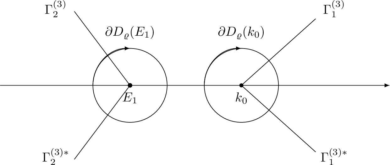
Using Lemma 4 and Lemma 5, a straightforward calculation yields the following proposition.
Proposition 14. For \(\xi\in\mathcal{T}_\mathrm{\uppercase{\romannumeral2}}\), the function \(V^{(err)}(\cdot)-I:\Gamma^{(err)}\to\mathbb{C}^{2\times2}\) lies in \(L^p\left(\Gamma^{(err)}\right)\) for \(p=1,2\), and uniformly for \(\xi\in\mathcal{T}_\mathrm{\uppercase{\romannumeral2}}\), it holds that \[\begin{align} &\Vert V^{(err)}(k)-I \Vert_{L^p\left(\Gamma^{(err)}\setminus\left(\overline{D_\varrho(E_1)}\cup \overline{D_\varrho(k_0)}\cup\mathbb{R}\right)\right)}= \mathcal{O}(\mathrm{e}^{-ct}), \\ &\Vert V^{(err)}(k)-I \Vert_{L^p\left(\partial D_\varrho(E_1)\cup \partial D_\varrho(k_0)\right)}=\mathcal{O}(t^{\gamma_p}),\\ &\Vert V^{(err)}(k)-I \Vert_{L^p\left(\mathbb{R}\setminus\left(\overline{D_\varrho(E_1)}\cup \overline{D_\varrho(k_0)}\right)\right)}=\mathcal{O}(t^{-1}),\\ &\Vert V^{(err)}(k)-I \Vert_{L^p\left(\Gamma^{(err)}\cap \left(D_\varrho(E_1)\cup D_\varrho(k_0)\right)\right)}=\mathcal{O}(t^{\omega_p}). \end{align}\] where \(c>0\), \[\begin{align} \gamma_1=-1/2,\;\gamma_2=-\frac{1}{4},\quad \omega_1=-\frac{3}{4},\;\omega_2=-\frac{1}{2}. \end{align}\] In particular, uniformly for \(\xi\in\mathcal{T}_\mathrm{\uppercase{\romannumeral2}}\), it holds that \[\Vert V^{(err)}(k)-I \Vert_{L^p\left(\Gamma^{(err)}\right)}=\mathcal{O}(t^{\gamma_p}), \quad p=1,2.\]
Proof. The proof is similar to that of Proposition 10. ◻
The solution for \(M^{(err)}\) can be given by \[\label{BCsolforErrorR3} M^{(err)}(k) = I + \frac{1}{2\pi \mathrm{i}} \int_{\Gamma^{(err)}} \frac{(I + \varpi(p))(V^{(err)}(p) - I)}{p - k} \mathop{}\!\mathrm{d}p,\tag{76}\] where \(\varpi\in L^{2}(\Gamma^{(err)})\) is the unique solution of \((1 - C_{V^{(err)}})\varpi = C_{V^{(err)}} I\). Analogous to the estimate 54 , we have \(\|C_{V^{(err)}}\|_{L^2(\Gamma^{(err)})} = \mathcal{O}(t^{-1/4})\), which implies that \(1 - C_{V^{(err)}}\) is invertible for large positive \(t\) in this case.
Moreover, by 76 , it follows that \[M^{(err)}(k)=I+\frac{M^{(err)}_1}{k}+\mathcal{O}(k^{-2}), \quad k\rightarrow\infty,\] where \[M^{(err)}_1=-\frac{1}{2\pi \mathrm{i}}\int_{\Gamma^{(err)}}\left(I + \varpi(z)\right)(V^{(err)}(z)-I)\mathop{}\!\mathrm{d}z.\] Then we obtain the following proposition.
Proposition 15. For \(\xi\in\mathcal{T}_\mathrm{\uppercase{\romannumeral2}}\), as \(t\rightarrow+\infty\), \[M^{(err)}_1=\frac{1}{2}\left(\frac{9}{2}\right)^{-\frac{1}{3}}(k_0-E_1)^{\frac{1}{3}}a(s)t^{-\frac{1}{3}} \begin{pmatrix}\mathrm{i}&-1\\-1&-\mathrm{i}\end{pmatrix}+\mathcal{O}(t^{-\frac{1}{2}}),\] where \(a(s)\) is defined as in 102 .
Proof. The definition of \(M^{(err)}_1\) in 56 implies that \[\begin{align} M^{(err)}_1=&-\frac{1}{2\pi \mathrm{i}}\oint_{\partial D_\varrho(E_1)}\left(V^{(err)}(p)-I\right)\mathop{}\!\mathrm{d}p+\mathcal{O}(t^{-1/2} )\\ =&-\frac{1}{2\pi \mathrm{i}}\oint_{\partial D_\varrho(E_1)}\frac{1}{\zeta(p)}P(p;\xi,t)\begin{pmatrix} \left(M_1^{P_{34}}(s)\right)_{11}&\left(M_1^{P_{34}}(s)\right)_{12}\\0&\left(M_1^{P_{34}}(s)\right)_{22} \end{pmatrix} P(p;\xi,t)^{-1}\mathop{}\!\mathrm{d}p+\mathcal{O}(t^{-1/2})\\ =&-\frac{1}{2\pi \mathrm{i}}\oint_{\partial D_\varrho(E_1)}\frac{1}{\zeta(p)}P(p;1,t)\begin{pmatrix} \left(M_1^{P_{34}}(s)\right)_{11}&t^{1/3}\left(M_1^{P_{34}}(s)\right)_{12}\\0&\left(M_1^{P_{34}}(s)\right)_{22} \end{pmatrix} P(p;1,t)^{-1}\mathop{}\!\mathrm{d}p+\mathcal{O}(t^{-1/2}). \end{align}\] Using the residue theorem and the definition of \(\zeta\) in 66 completes the proof. ◻
4.6 Proof of the part (\(\mathrm{\uppercase{\romannumeral2}}\)) of Theorem 1↩︎
By tracing back the transformations 60 , 62 , 63 and 75 , we conclude that, for \(k\in\mathbb{C}\setminus\left(\Gamma^{(3)}\cap D_\varrho(E_1)\cap D_\varrho(k_0)\right)\), \[M(k)=\mathrm{e}^{\mathrm{i}tg_{\mathrm{\uppercase{\romannumeral2}},\infty}(\xi)\sigma_3}D_{\mathrm{\uppercase{\romannumeral2}},\infty}(\xi)^{-\sigma_3}M^{(err)}(k)M^{(\infty)}(k)D_{\mathrm{\uppercase{\romannumeral2}}}^{\sigma_3}(k)G^{-1}(k)\mathrm{e}^{-\mathrm{i}t(g_{\mathrm{\uppercase{\romannumeral2}}}(k)-\theta(k))\sigma_3},\] where \(g_{\mathrm{\uppercase{\romannumeral1}}}\), \(D_{\mathrm{\uppercase{\romannumeral1}}}\), \(M^{(err)}\), \(M^{(\infty)}\) and \(G\) are defined in 58 , 61 , 75 , [RHP:Minfty32RII] and 64 respectively. From the reconstruction formula stated in 24 , we obtain that Together with the reconstruction formula stated in 24 , we obtain \[\begin{align} u(x,t)=2\mathrm{i}\mathrm{e}^{2\mathrm{i}tg_{\mathrm{\uppercase{\romannumeral2}},\infty}(\xi)} D_{\mathrm{\uppercase{\romannumeral2}},\infty}^{-2}(\xi)\left[(M^{(err)}_1)_{12}+\lim_{k\rightarrow\infty}k\left(M^{(\infty)}(k)\right)_{12}\right]. \end{align}\] Based on item (a) of Lemma [lemma:minfty32for32T2] and Proposition 15, we obtain part () of Theorem 1.
5 Asymptotic analysis of the RH problem for \(M\) in \(\mathcal{T}_{\mathrm{\uppercase{\romannumeral3}}}\)↩︎
As \(\xi\) approaches \(4\beta+4\alpha\) in the right most region, the saddle point \(k_0=-\frac{\xi}{4}\) of \(\theta(k)\) tends to \(E_1\) with a certain speed; see Figure 11. On the other hand, \(|r(k)|\equiv1\) for \(k\in[E_1,E_2]\), thus the diagonal entry \((1-r(k)r^*(k))^{-1}\) in the factorization 25 becomes unbounded at the same time. As a consequence, a new transition zone appears between region \(\mathcal{T}_{\mathrm{\uppercase{\romannumeral2}}}\) and the right most region, which is called the collisionless shock region.
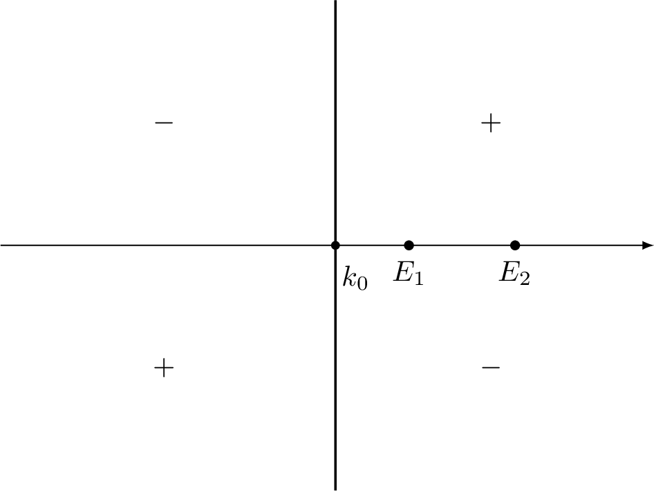
5.1 First transformation: \(M\rightarrow M^{(1)}\)↩︎
In this section, we rewrite the phase factor \(\mathrm{e}^{\mathrm{i}t\theta(k)}\) into a simpler way which relocates the saddle point \(k_0\) to \(-1\) and \(E_1\) to \(0\) respectively. Introduce the following changes of variables \[\label{equ:def32z32tau} z=\frac{k-E_1}{E_1-k_0},\quad \tau=\frac{t[\xi-4(\alpha+\beta)]^2}{8}.\tag{77}\] Denote by \(\tau\hat{\theta}(z)=\tau\hat{\theta}(z;\xi):=t\theta(k(z);\xi)\), which implies that \[\tau\hat{\theta}(z)=\tau z^2+2\tau z+2tE_1^2+xE_1.\] This operation provokes us to consider the RH problem in the \(z\)-plane. We introduce a new matrix-valued function \(M^{(1)}\) by \[\label{def:M132RIII} M^{(1)}(z)= M^{(1)}(z;x,t):=M(k(z))\mathrm{e}^{-\mathrm{i}\left(2tE_1^2+xE_1\right)\sigma_3}.\tag{78}\] Then the RH problem for \(M^{(1)}\) reads as follows:
RH problem 17.
\(M^{(1)}(z)\) is holomorphic for \(k\in\mathbb{C}\setminus\mathbb{R}\).
\(M^{(1)}(z)\) has continuous boundary values \(M_{\pm}^{(1)}(z)\) on \(\mathbb{R}\) with the jump condition \[M^{(1)}_{+}(z)=M^{(1)}_{-}(z)V^{(1)}(z), \quad k\in\mathbb{R},\] where \[\label{equ:jump32V132RIII} V^{(1)}(z)= \begin{pmatrix}1-\hat{r}(z)\hat{r}^*(z) & \hat{r}^*(z)\mathrm{e}^{-2\mathrm{i}\tau(z^2+2z)}\\ -\hat{r}(z)\mathrm{e}^{2\mathrm{i}\tau(z^2+2z)} & 1\end{pmatrix}, \quad z\in\mathbb{R}.\qquad{(26)}\] Here, \(\hat{r}(z):=r(k(z))=r[(E_1-k_0)z+E_1)]\).
As \(k\rightarrow\infty\) in \(\mathbb{C}\setminus\mathbb{R}\), we have \(M^{(1)}(z)=I+\mathcal{O}(z^{-1})\).
5.2 Second transformation: \(M^{(1)}\rightarrow M^{(2)}\)↩︎
In this section, we introduce the \(g\)-function to further analyze the RH problem For \(M^{(1)}(z)\).
We define the hyperelliptic surface \(\mathcal{M}\) as the set of all points \(P:=(w,z)\in\mathbb{C}^2\) such that \[\label{equ:def32of32w40z41} w^2=(z^2-a^2)(z^2-b^2)\tag{79}\] together with two points \(\infty^+\) and \(\infty^-\) at infinity which make the surface compact, where \(0<a<1<b\). \(\mathcal{M}\) is a Riemann surface of genus \(1\) and the upper (resp.lower) sheet is characterized by \(w=z^2+\mathcal{O}(z)\) (resp.\(w=-z^2+\mathcal{O}(z)\)). Its branch cuts and the canonical bases \(\{a_1,b_1\}\) are illustrated in Figure 12.
![Figure 12: The homology basis of the Riemann surface \mathcal{M} associated withw(z) = \sqrt{(z^2 - a^2)(z^2 -b^2)}. The a_1-cycle is closed counterclockwise oriented simple loop around the cut [a,b] and the b_1-cycle starts on the upper sheet of the cut [a,b], goes to the cut [-b,-a], proceeds to the lower sheet, and then returns to the starting point.](/article/2606.26911/_pdflatex/skdfuapo.png "fig:")
Therefore, the \(g\)-function for \(\xi\in\mathcal{T}_{\mathrm{\uppercase{\romannumeral3}}}\) is defined by \[\label{equ:gIII} g_{\mathrm{\uppercase{\romannumeral3}}}(z)=g_{\mathrm{\uppercase{\romannumeral3}}}(z;\xi):=4\int_{-b}^z\frac{(p^2-1)(p+1)}{w(p)}\mathop{}\!\mathrm{d}p+B_1,\tag{80}\] where \[\begin{align} & B_1=2\int_{-a}^a\frac{(p^2-1)(p+1)}{w(p)}\mathop{}\!\mathrm{d}p,\tag{81}\\ & a^2+b^2=2.\tag{82} \end{align}\] and the branch of the square root is chosen such that \(w(z)=\sqrt{(z^2-a^2)(z^2-b^2)}>0\) for \(z\in\mathbb{R},\;k\gg0\). The restriction on parameters \(a,b\) in 82 makes sure \(g^\prime_{\mathrm{\uppercase{\romannumeral3}}}(z)=4(z+1)+\mathcal{O}(z^{-2})\). To determine the parameters \(a\) and \(b\) uniquely, we need the following Proposition which is also essential in decompose the jump matrix on the gap \((-a,a)\) as \(t\to+\infty\):
Proposition 16. For \(\xi\in\mathcal{T}_{\mathrm{\uppercase{\romannumeral3}}}\), there exists unique \(a\) and \(b\) for \(0<a<1<b\) which satisfies 82 and the following equation for every \(t>0\): \[\label{equ:unique32of32d} (E_1-k_0)^{\frac{1}{2}}\mathrm{e}^{8\tau\int_{-b}^{-a}\frac{|p^2-1||p+1|}{|p^2-a^2|^{1/2}|p^2-b^2|^{1/2}}\mathop{}\!\mathrm{d}p}=1.\qquad{(27)}\]
The proof of this proposition can be found in Appendix 7. From the definition of \(g_{\mathrm{\uppercase{\romannumeral3}}}\) in 80 , the following Proposition is straightforward.
Proposition 17. The function \(g_{\mathrm{\uppercase{\romannumeral3}}}\) defined in 80 satisfies the following properties.
\(g_{\mathrm{\uppercase{\romannumeral3}}}(z)\) is holomorphic for \(z \in \mathbb{C} \setminus[-b, b]\).
As \(z \to \infty\) in \(\mathbb{C} \setminus[-b, b]\), we have \(g_{\mathrm{\uppercase{\romannumeral3}}}(z)=2(z^2+2z)+g_{\mathrm{\uppercase{\romannumeral3}},\infty}(\xi)+\mathcal{O}\left(z^{-1}\right)\), where \(g_{\mathrm{\uppercase{\romannumeral3}},\infty}(\xi)\in\mathbb{R}\) is a finite real number independent of \(z\).
\(g_{\mathrm{\uppercase{\romannumeral3}}}(z)\) satisfies the following jump relations on \([-b, b]\): \[\begin{align} &g_{\mathrm{\uppercase{\romannumeral3}},+}(z)+g_{\mathrm{\uppercase{\romannumeral3}},-}(z)=-2B_1 , && z \in(a, b), \\ &g_{\mathrm{\uppercase{\romannumeral3}},+}(z)+g_{\mathrm{\uppercase{\romannumeral3}},-}(z)=2B_1, && z\in(-b,-a), \\ &g_{\mathrm{\uppercase{\romannumeral3}},+}(z)-g_{\mathrm{\uppercase{\romannumeral3}},-}(z)=A_1, && z \in(-a, a), \end{align}\] where \[\label{equ:def32of32A951} A_1=-8\mathrm{i}\int_{-b}^{-a}\frac{|p+1|^2|p-1|}{|p^2-a^2|^{1/2}|p^2-b^2|^{1/2}} \mathop{}\!\mathrm{d}p\qquad{(28)}\] and \(B_1\) is given in 81 .
With the help of function \(g_{\mathrm{\uppercase{\romannumeral3}}}\) defined in 80 , we introduce a new matrix-valued function \(M^{(2)}\) by \[\label{def:M232RIII} M^{(2)}(z)= M^{(2)}(z;x,t):=\mathrm{e}^{-\mathrm{i}tg_{\mathrm{\uppercase{\romannumeral3}},\infty}(\xi)\sigma_3}M^{(1)}(z)\mathrm{e}^{\mathrm{i}t\left[g_{\mathrm{\uppercase{\romannumeral3}}}(z)-(z^2+2z)\right]\sigma_3}.\tag{83}\] Then the RH problem for \(M^{(2)}\) reads as follows:
RH problem 18.
\(M^{(2)}(z)\) is holomorphic for \(z\in\mathbb{C}\setminus\mathbb{R}\).
\(M^{(2)}(z)\) has continuous boundary values \(M_{\pm}^{(2)}(z)\) on \(\mathbb{R}\) with the jump condition \[M^{(2)}_{+}(z)=M^{(2)}_{-}(z)V^{(2)}(z), \quad z\in\mathbb{R},\] where \[\label{equ:jump32V232RIII} V^{(2)}(z)= \begin{pmatrix}\left(1-\hat{r}(z)\hat{r}^*(z)\right)\mathrm{e}^{\mathrm{i}\tau\left(g_{\mathrm{\uppercase{\romannumeral3}},+}(z)-g_{\mathrm{\uppercase{\romannumeral3}},-}(z)\right)} & \hat{r}^*(z)\mathrm{e}^{-\mathrm{i}\tau\left(g_{\mathrm{\uppercase{\romannumeral3}},+}(z)+g_{\mathrm{\uppercase{\romannumeral3}},-}(z)\right)}\\ -\hat{r}(z)\mathrm{e}^{\mathrm{i}\tau\left(g_{\mathrm{\uppercase{\romannumeral3}},+}(z)+g_{\mathrm{\uppercase{\romannumeral3}},-}(z)\right)} & \mathrm{e}^{-\mathrm{i}\tau\left(g_{\mathrm{\uppercase{\romannumeral3}},+}(z)-g_{\mathrm{\uppercase{\romannumeral3}},-}(z)\right)}\end{pmatrix}.\qquad{(29)}\]
As \(z\rightarrow\infty\) in \(\mathbb{C}\setminus\mathbb{R}\), we have \(M^{(2)}(z)=I+\mathcal{O}(z^{-1})\).

By the signature table of \(\mathop{\mathrm{Im}}g_{\mathrm{\uppercase{\romannumeral3}}}\) in Figure 13 and the jump condition in item (c) of Proposition 17, the jump matrix \(V^{(2)}\) of \(M^{(2)}\) defined in ?? admits the following upper/lower triangular factorizations: \[\label{equ:factor32gIII} V^{(2)}(z)=\begin{cases} \begin{pmatrix} 1 & 0 \\-\hat{r}_2^*(z)\mathrm{e}^{2\mathrm{i}\tau g_{\mathrm{\uppercase{\romannumeral3}}}(z)} & 1 \end{pmatrix}\left(1-\hat{r}(z)\hat{r}^*(z)\right)^{\sigma_3}\begin{pmatrix} 1 & \hat{r}_2(z)\mathrm{e}^{-2\mathrm{i}\tau g_{\mathrm{\uppercase{\romannumeral3}}}(z)}\\ 0 & 1 \end{pmatrix}, &z\in(-\infty,-b),\\ \begin{pmatrix}\left(1-\hat{r}(z)\hat{r}^*(z)\right)\mathrm{e}^{\mathrm{i}\tau\left(g_{\mathrm{\uppercase{\romannumeral3}},+}(z)-g_{\mathrm{\uppercase{\romannumeral3}},-}(z)\right)} & \hat{r}^*(z)\mathrm{e}^{-2\mathrm{i}\tau B_1}\\ -\hat{r}(z)\mathrm{e}^{2\mathrm{i}\tau B_1} & \mathrm{e}^{-\mathrm{i}\tau\left(g_{\mathrm{\uppercase{\romannumeral3}},+}(z)-g_{\mathrm{\uppercase{\romannumeral3}},-}(z)\right)}\end{pmatrix}, &z\in(-b,-a),\\ \begin{pmatrix} 1 & 0 \\-\hat{r}_2^*(z)\mathrm{e}^{2\mathrm{i}\tau g_{\mathrm{\uppercase{\romannumeral3}},-}(z)} & 1 \end{pmatrix}\left[\left(1-\hat{r}(z)\hat{r}^*(z)\right)\mathrm{e}^{\mathrm{i}\tau A_1}\right]^{\sigma_3}\begin{pmatrix} 1 & \hat{r}_2(z)\mathrm{e}^{-2\mathrm{i}\tau g_{\mathrm{\uppercase{\romannumeral3}},+}(z)}\\ 0 & 1 \end{pmatrix}, &z\in(-a,a),\\ \begin{pmatrix}\left(1-\hat{r}(z)\hat{r}^*(z)\right)\mathrm{e}^{\mathrm{i}\tau\left(g_{\mathrm{\uppercase{\romannumeral3}},+}(z)-g_{\mathrm{\uppercase{\romannumeral3}},-}(z)\right)} & \hat{r}^*(z)\mathrm{e}^{2\mathrm{i}\tau B_1}\\ -\hat{r}(z)\mathrm{e}^{-2\mathrm{i}\tau B_1} & \mathrm{e}^{-\mathrm{i}\tau\left(g_{\mathrm{\uppercase{\romannumeral3}},+}(z)-g_{\mathrm{\uppercase{\romannumeral3}},-}(z)\right)}\end{pmatrix}, &z\in(a,b),\\ \begin{pmatrix} 1 & \hat{r}^*(z)\mathrm{e}^{-2\mathrm{i}\tau g_{\mathrm{\uppercase{\romannumeral3}}}(z)} \\ 0 & 1\end{pmatrix}\begin{pmatrix} 1 & 0 \\ -\hat{r}(z)\mathrm{e}^{2\mathrm{i}\tau g_{\mathrm{\uppercase{\romannumeral3}}}(z)} & 1\end{pmatrix}, &z\in(b,+\infty), \end{cases}\tag{84}\] where \(\hat{r}_2(z)=\frac{\hat{r}^*(z)}{1-\hat{r}(z)\hat{r}^*(z)}\).
5.3 Third transformation: \(M^{(2)}\rightarrow M^{(3)}\)↩︎
To eliminate the diagonal matrix for \(z\in(-\infty,-b)\) in 84 , we introduce a complex-valued function \(\delta(z):=\delta(z;\xi)\) which reads \[\label{equ:definition32TIII32delta} \delta(z)=\exp\left[\frac{1}{2\pi\mathrm{i}}\int_{-\infty}^{-b}\frac{\log(1-\hat{r}(\zeta)\hat{r}^*(\zeta))}{\zeta-z}\mathop{}\!\mathrm{d}\zeta\right],\quad z\in\mathbb{C}\setminus(-\infty,-b].\tag{85}\] The following proposition follows immediately.
Proposition 18. The function \(\delta(z)\) defined in 85 has the following properties:
\(\delta(z)\) and \(\delta(z)^{-1}\) are bounded and analytic functions of \(z \in \mathbb{C} \setminus(-\infty, -b]\) with continuous boundary values on \((-\infty,-b)\).
\(\delta(z)\) satisfies the following jump condition \[\delta_{+}(z)=\delta_{-}(z)\left[1-\hat{r}(z)\hat{r}^*(z)\right], \quad z \in(-\infty,-b).\]
As \(z\to\infty\), we have \(\delta(z)=1+\mathcal{O}(z^{-1})\).
With the help of function \(\delta\), we define a new matrix-valued function \(M^{(3)}\) by \[\label{def:M332RIII} M^{(3)}(z)=M^{(3)}(z;x,t):= M^{(2)}(z)\delta(z)^{-\sigma_3},\tag{86}\] then RH problem for \(M^{(3)}\) reads as follows:
RH problem 19.
\(M^{(3)}(z)\) is holomorphic for \(z\in\mathbb{C}\setminus\mathbb{R}\).
\(M^{(3)}(z)\) has continuous boundary values \(M_{\pm}^{(3)}(z)\) on \(\mathbb{R}\) with the jump condition \[M^{(3)}_{+}(z)=M^{(3)}_{-}(z)V^{(3)}(z), \quad z\in\mathbb{R},\] where \[\label{equ:jump32V332RIII} V^{(3)}(z)= \begin{cases} \begin{pmatrix} 1 & 0 \\-\hat{r}_2^*\delta^{-2}_-\mathrm{e}^{2\mathrm{i}\tau g_{\mathrm{\uppercase{\romannumeral3}}}} & 1 \end{pmatrix}\begin{pmatrix} 1 & \hat{r}_2\delta_+^2\mathrm{e}^{-2\mathrm{i}\tau g_{\mathrm{\uppercase{\romannumeral3}}}}\\ 0 & 1 \end{pmatrix}, &z\in(-\infty,-b),\\ \begin{pmatrix}\left(1-\hat{r}\hat{r}^*\right)\mathrm{e}^{\mathrm{i}\tau\left(g_{\mathrm{\uppercase{\romannumeral3}},+}-g_{\mathrm{\uppercase{\romannumeral3}},-}\right)} & \hat{r}^*\delta^{2}\mathrm{e}^{-2\mathrm{i}\tau B_1}\\ -\hat{r}\delta^{-2}\mathrm{e}^{2\mathrm{i}\tau B_1} & \mathrm{e}^{-\mathrm{i}\tau\left(g_{\mathrm{\uppercase{\romannumeral3}},+}-g_{\mathrm{\uppercase{\romannumeral3}},-}\right)}\end{pmatrix}, &z\in(-b,-a),\\ \begin{pmatrix} 1 & 0 \\-\hat{r}_2^*\delta^{-2}\mathrm{e}^{2\mathrm{i}\tau g_{\mathrm{\uppercase{\romannumeral3}},-}} & 1 \end{pmatrix}\left[\left(1-\hat{r}\hat{r}^*\right)\mathrm{e}^{\mathrm{i}\tau A_1}\right]^{\sigma_3}\begin{pmatrix} 1 & \hat{r}_2\delta^{2}\mathrm{e}^{-2\mathrm{i}\tau g_{\mathrm{\uppercase{\romannumeral3}},+}}\\ 0 & 1 \end{pmatrix}, &z\in(-a,a),\\ \begin{pmatrix}\left(1-\hat{r}\hat{r}^*\right)\mathrm{e}^{\mathrm{i}\tau\left(g_{\mathrm{\uppercase{\romannumeral3}},+}-g_{\mathrm{\uppercase{\romannumeral3}},-}\right)} & \hat{r}^*\delta^{2}\mathrm{e}^{2\mathrm{i}\tau B_1}\\ -\hat{r}\delta^{-2}\mathrm{e}^{-2\mathrm{i}\tau B_1} & \mathrm{e}^{-\mathrm{i}\tau\left(g_{\mathrm{\uppercase{\romannumeral3}},+}-g_{\mathrm{\uppercase{\romannumeral3}},-}\right)}\end{pmatrix}, &z\in(a,b),\\ \begin{pmatrix} 1 & \hat{r}^*\delta^{2}\mathrm{e}^{-2\mathrm{i}\tau g_{\mathrm{\uppercase{\romannumeral3}}}} \\ 0 & 1\end{pmatrix}\begin{pmatrix} 1 & 0 \\ -\hat{r}\delta^{-2}\mathrm{e}^{2\mathrm{i}\tau g_{\mathrm{\uppercase{\romannumeral3}}}} & 1\end{pmatrix}, &z\in(b,+\infty). \end{cases}\qquad{(30)}\]
As \(z\rightarrow\infty\) in \(\mathbb{C}\setminus\mathbb{R}\), we have \(M^{(3)}(z)=I+\mathcal{O}(z^{-1})\).
5.4 Fourth transformation: \(M^{(3)}\rightarrow M^{(4)}\)↩︎
The aim of the fourth transformation is to open lenses in regions \(U^{(4)}_j,U^{(4)*}_j,\;j=1,2,3\), which are illustrated in Figure 14. Following the same operations given by Proposition 7 and Proposition 8, we can obtain the analytic approximation for the spectral function \(\hat{r}\) in region \(U^{(4)}_1\) (denoted as \(\hat{r}_a\)), as well as the analytic approximation for \(\hat{r}_2\) in regions \(U^{(4)}_2\) and \(U^{(4)}_3\) (denoted as \(\hat{r}_{2,a}\)).
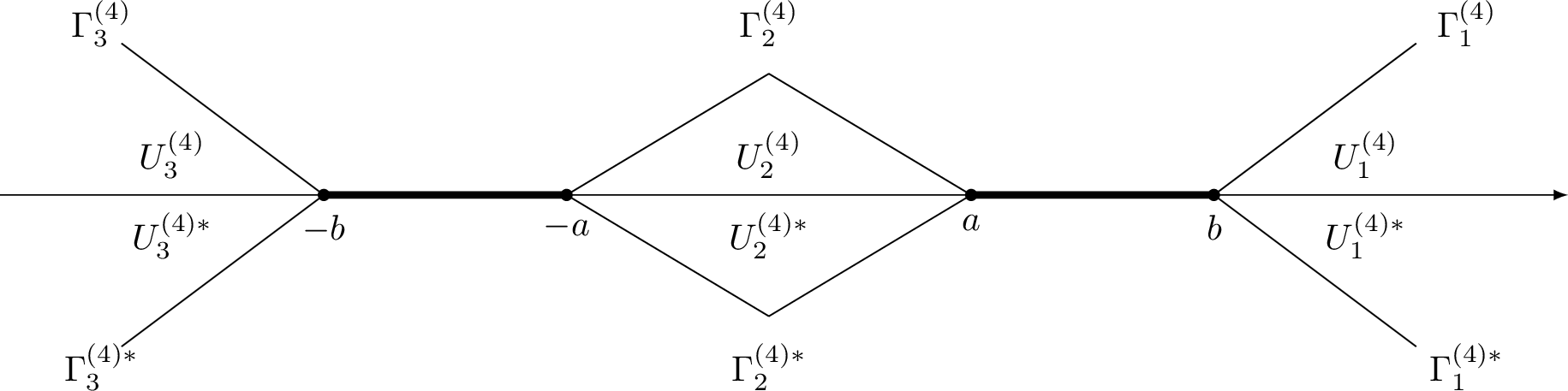
Now we are ready to define matrix-valued function \(M^{(4)}\) by \[\label{def:M432RIII} M^{(4)}(z)=M^{(4)}(z;x,t):=M^{(3)}(k)\delta^{\sigma_3}(z)G(z)\delta(z)^{-\sigma_3},\tag{87}\] where \[\label{def:G32TIII} G(z):= \begin{cases} \begin{pmatrix}1 & 0 \\ \hat{r}_a\mathrm{e}^{2\mathrm{i}tg_{\mathrm{\uppercase{\romannumeral3}}}} & 1\end{pmatrix}, &z\in U^{(4)}_1, \\ \begin{pmatrix}1 & \hat{r}_a^{*}\mathrm{e}^{-2\mathrm{i}tg_\mathrm{\uppercase{\romannumeral3}}} \\ 0 & 1\end{pmatrix}, &z\in U_1^{(4)*}, \\ \begin{pmatrix}1 & -\hat{r}_{2,a}\mathrm{e}^{-2\mathrm{i}tg_\mathrm{\uppercase{\romannumeral3}}} \\ 0 & 1\end{pmatrix}, &z\in U_2^{(4)}\cup U_3^{(4)},\\ \begin{pmatrix}1 & 0 \\ -\hat{r}^*_{2,a}\mathrm{e}^{2\mathrm{i}tg_\mathrm{\uppercase{\romannumeral3}}} & 1\end{pmatrix}, & z\in U_2^{(4)*}\cup U_3^{(4)*},\\ I, &\textrm{elsewhere}. \end{cases}\tag{88}\] Here, the domains \(U^{(4)}_j\), \(j=1,2,3\) are illustrated in Figure 14.
Therefore, the RH problem for \(M^{(4)}\) reads as follows:
RH problem 20.
\(M^{(4)}(z)\) is holomorphic for \(z\in\mathbb{C}\setminus\Gamma^{(4)}\), where \(\Gamma^{(4)}:=\cup_{j=1}^{3}(\Gamma^{(4)}_j\cup\Gamma_j^{(4)*})\cup\mathbb{R}\); see Figure 14 for an illustration.
\(M^{(4)}(z)\) has continuous boundary values \(M_{\pm}^{(4)}(z)\) on \(z\in \Gamma^{(4)}\) with the jump condition \[M^{(4)}_{+}(z)= M^{(4)}_{-}(z)V^{(4)}(z),\] where \[\label{equ:jump32V432RIII} V^{(4)}(z)= \begin{cases} \begin{pmatrix} 1 & 0 \\ -\hat{r}_a\delta^{-2}\mathrm{e}^{2\mathrm{i}\tau g_{\mathrm{\uppercase{\romannumeral3}}}} & 1\end{pmatrix}, &z\in\Gamma^{(4)}_1, \\ \begin{pmatrix} 1 & \hat{r}_a^*\delta^{2}\mathrm{e}^{-2\mathrm{i}\tau g_{\mathrm{\uppercase{\romannumeral3}}}} \\ 0 & 1\end{pmatrix}, & z\in\Gamma^{(4)*}_1, \\ \begin{pmatrix} 1 & \hat{r}_{2,a}\delta^{2}\mathrm{e}^{-2\mathrm{i}\tau g_{\mathrm{\uppercase{\romannumeral3}}}}\\ 0 & 1 \end{pmatrix}, &z\in\Gamma^{(4)}_2\cup\Gamma^{(4)}_3, \\ \begin{pmatrix} 1 & 0 \\-\hat{r}_{2,a}^*\delta^{-2}\mathrm{e}^{2\mathrm{i}\tau g_{\mathrm{\uppercase{\romannumeral3}}}} & 1 \end{pmatrix}, & z\in\Gamma^{(4)*}_2\cup\Gamma^{(4)*}_3, \\ \begin{pmatrix}1-\hat{r}_r\hat{r}_r^* & \hat{r}_r^*\delta^2\mathrm{e}^{-2\mathrm{i}\tau g_{\mathrm{\uppercase{\romannumeral3}}}}\\ -\hat{r}_r \delta^{-2}\mathrm{e}^{2\mathrm{i}\tau g_{\mathrm{\uppercase{\romannumeral3}}}} & 1\end{pmatrix},&z\in(b,+\infty),\\ \begin{pmatrix}1 & \hat{r}_r^*\delta_+^2\mathrm{e}^{-2\mathrm{i}\tau g_{\mathrm{\uppercase{\romannumeral3}}}}\\ -\hat{r}_r \delta_-^{-2}\mathrm{e}^{2\mathrm{i}\tau g_{\mathrm{\uppercase{\romannumeral3}}}} & 1-\hat{r}_r\hat{r}_r^*\end{pmatrix},&z\in(-\infty,-b),\\ \begin{pmatrix}\left(1-\hat{r}\hat{r}^*\right)\mathrm{e}^{\mathrm{i}\tau\left(g_{\mathrm{\uppercase{\romannumeral3}},+}-g_{\mathrm{\uppercase{\romannumeral3}},-}\right)} & \hat{r}^*\delta^{2}\mathrm{e}^{2\mathrm{i}\tau B_1}\\ -\hat{r}\delta^{-2}\mathrm{e}^{-2\mathrm{i}\tau B_1} & \mathrm{e}^{-\mathrm{i}\tau\left(g_{\mathrm{\uppercase{\romannumeral3}},+}-g_{\mathrm{\uppercase{\romannumeral3}},-}\right)}\end{pmatrix}, &z\in(a,b),\\ \begin{pmatrix}\left(1-\hat{r}\hat{r}^*\right)\mathrm{e}^{\mathrm{i}\tau\left(g_{\mathrm{\uppercase{\romannumeral3}},+}-g_{\mathrm{\uppercase{\romannumeral3}},-}\right)} & \hat{r}^*\delta^{2}\mathrm{e}^{-2\mathrm{i}\tau B_1}\\ -\hat{r}\delta^{-2}\mathrm{e}^{2\mathrm{i}\tau B_1} & \mathrm{e}^{-\mathrm{i}\tau\left(g_{\mathrm{\uppercase{\romannumeral3}},+}-g_{\mathrm{\uppercase{\romannumeral3}},-}\right)}\end{pmatrix}, &z\in(-b,-a),\\ \begin{pmatrix} 1 & 0 \\-\hat{r}_{2,r}^*\delta^{-2}\mathrm{e}^{2\mathrm{i}\tau g_{\mathrm{\uppercase{\romannumeral3}},-}} & 1 \end{pmatrix}\left[\left(1-\hat{r}\hat{r}^*\right)\mathrm{e}^{\mathrm{i}\tau A_1}\right]^{\sigma_3}\begin{pmatrix} 1 & \hat{r}_{2,r}\delta^{2}\mathrm{e}^{-2\mathrm{i}\tau g_{\mathrm{\uppercase{\romannumeral3}},+}}\\ 0 & 1 \end{pmatrix}, &z\in(-a,a). \end{cases}\qquad{(31)}\]
As \(z\rightarrow\infty\) in \(\mathbb{C}\setminus\Gamma^{(4)}\), we have \(M^{(4)}(z)=I+\mathcal{O}(z^{-1})\).
5.5 Analysis of RH problem for \(M^{(4)}\)↩︎
As \(t\to+\infty\), RH problem \(M^{(4)}(z)\) for \(\xi\in\mathcal{T}_{\mathrm{\uppercase{\romannumeral3}}}\) can be reduced to the following RH problem.
RH problem 21.
\(M^{(mod)}(z)\) is holomorphic for \(z\in\mathbb{C}\setminus[-b,b]\).
\(M^{(mod)}(z)\) has continuous boundary values \(M_{\pm}^{(mod)}(z)\) on \(z\in (-b,b)\) with the jump condition \[M^{(mod)}_{+}(z)= M^{(mod)}_{-}(z)V^{(mod)}(z),\] where \[\label{equ:jump32Vmod32RIII} V^{(mod)}(z)= \begin{cases} \begin{pmatrix}0 &\overline{q_{1,0}}\delta^2(0)\mathrm{e}^{2\mathrm{i}\tau B_1}\\ -q_{1,0}\delta^{-2}(0)\mathrm{e}^{-2\mathrm{i}\tau B_1} &0\end{pmatrix}, &z\in(a,b),\\ \begin{pmatrix}0 & \overline{q_{1,0}}\delta^2(0)\mathrm{e}^{-2\mathrm{i}\tau B_1}\\-q_{1,0}\delta^{-2}(0)\mathrm{e}^{2\mathrm{i}\tau B_1} & 0\end{pmatrix}, &z\in(-b,-a),\\ \begin{pmatrix} 2\gamma z^{\frac{1}{2}} &0\\0&\frac{1}{2\gamma z^{\frac{1}{2}}} \end{pmatrix}, &z\in(-a,a), \end{cases}\qquad{(32)}\] where \(\gamma=\frac{\mathrm{i}(q_{1,0}\overline{q_{1,1}}+\overline{q_{1,0}}q_{1,1})}{2}\).
As \(z\rightarrow\infty\) in \(\mathbb{C}\setminus[-b,b]\), we have \(M^{(mod)}(z)=I+\mathcal{O}(z^{-1})\).
Proof. We only need to prove the jump condition in ?? . As \(t\to+\infty\), It can be deduced from 77 and item (d) of Proposition 4 that \[\label{sim32r95232TIII} |\hat{r}(z)|\sim1,\quad |1-\hat{r}(z)\hat{r}^*(z)|\sim2\gamma(E_1-k_0)^{\frac{1}{2}}z^{\frac{1}{2}},\quad \delta(z)\sim\delta(0).\tag{89}\]
For \(z\in(-a,a)\), from ?? and Proposition 16, it can be calculated that \[\left[1-\hat{r}(z)\hat{r}^*(z)\right]\mathrm{e}^{\mathrm{i}\tau A_1}\sim2\gamma(E_1-k_0)^{\frac{1}{2}}\mathrm{e}^{8\tau I(a,b)}z^{\frac{1}{2}}=2\gamma z^{\frac{1}{2}}.\] Moreover, the decay property of \(\hat{r}_{2,r}\) ensures that the non-diagonal part tends to \(0\) as \(t\to+\infty\).
For \(z\in(a,b)\), the diagonal part can be deduced from 89 . As to the non-diagonal part, when \(t\to+\infty\), we have \[\left[1-\hat{r}(z)\hat{r}^*(z)\right]\mathrm{e}^{\mathrm{i}\tau\left[g_{\mathrm{\uppercase{\romannumeral3}},+}(z)-g_{\mathrm{\uppercase{\romannumeral3}},-}(z)\right]}=2\gamma(E_1-k_0)^{\frac{1}{2}}\mathrm{e}^{8\tau\int_{-b}^{z}\frac{|p^2-1||p+1|}{|p^2-a^2|^{1/2}|p^2-b^2|^{1/2}}\mathop{}\!\mathrm{d}p}z^{\frac{1}{2}}\to0.\] Together with the signs of \(\mathop{\mathrm{Im}}g_{\mathrm{\uppercase{\romannumeral3}}}\) for \(\xi\in\mathcal{T}_{\mathrm{\uppercase{\romannumeral3}}}\) in Figure 13 arrive at the jump matrix of \(V^{(mod)}(z)\) for \(z\in(a,b)\).
For \(z\in\Gamma^{(3)}\setminus(-b,b)\), jump matrix \(V^{(4)}(z)\) tends to \(I\) immediately from the signs of \(\mathop{\mathrm{Im}}g_{\mathrm{\uppercase{\romannumeral3}}}\) for \(\xi\in\mathcal{T}_{\mathrm{\uppercase{\romannumeral3}}}\). ◻
To make the jump across the gap \((-a,a)\) constant in \(z\) and simplifies that of the two cuts, we define a new function \(h(z):=h(z;\xi)\) by \[\label{equ:def32of32h} \begin{align} h(z)=\frac{w(z)}{2\pi\mathrm{i}}&\left[\int_{-a}^a\frac{-\mathrm{i}\log(2\gamma p^{\frac{1}{2}})}{(p-z)w(p)}\mathop{}\!\mathrm{d}p+\int_a^b\frac{\Delta_0+\arg q_{1,0}+2\mathrm{i}\log\delta(0)}{(p-z)w_+(p)}\mathop{}\!\mathrm{d}p\right.\\ &\left.+\int_{-b}^{-a}\frac{-\Delta_0+\arg q_{1,0}+2\mathrm{i}\log\delta(0)}{(p-z)w_+(p)}\mathop{}\!\mathrm{d}p\right], \end{align}\tag{90}\] where \(w(z)\) is defined by 79 and \[\label{equ:def32of32delta0} \Delta_0=\left(2\int_a^b\frac{\mathop{}\!\mathrm{d}p}{w_+(p)}\right)^{-1}\int_{-a}^a\frac{\mathrm{i}\log(2\gamma p^{\frac{1}{2}})}{w(p)}\mathop{}\!\mathrm{d}p\tag{91}\] is a real number. By using the Sokhotski-Plemelj formula, we can obtain the following proposition for \(h\).
Proposition 19. The function \(h\) defined in 90 satisfies the following properties:
\(h(z)\) is holomorphic for \(z \in \mathbb{C} \setminus[-b, b]\).
\(h(z)\) satisfies the following jump conditions \[\begin{align} &h_{+}(z)-h_{-}(z)=-\mathrm{i}\log \left(2\gamma z^{1/2}\right), && z \in(-a, a), \\ &h_{+}(z)+h_{-}(z)=\Delta_0+\arg q_{1,0}+2\mathrm{i}\log\delta(0), && z \in(a, b), \\ &h_{+}(z)+h_{-}(z)=-\Delta_0+\arg q_{1,0}+2\mathrm{i}\log\delta(0), && z\in(-b,-a), \end{align}\] where \(\Delta_0\) is given in 91 .
As \(z \to \infty\) in \(\mathbb{C} \setminus[-b, b]\), we have \(h(z)=\mathcal{O}\left(z^{-1}\right)\).
With the help of the function \(h\), we can eliminate the jump on \((-a,a)\) and obtain a global RH problem \(M^{(\infty)}\). Define \[\label{equ:defMinfty32RIII} M^{(\infty)}(z)=M^{(mod)}(z)\mathrm{e}^{-\mathrm{i}h(z)\sigma_3}.\tag{92}\] By RH problem 21 and Proposition 19, \(M^{(\infty)}\) satisfies the following RH problem:
RH problem 22.
\(M^{(\infty)}(z)\) is holomorphic for \(z \in \mathbb{C} \setminus([-b,-a] \cup[a, b])\).
\(M^{(\infty)}(z)\) has continuous boundary values \(M_{\pm}^{(\infty)}(z)\) on \(z \in(-b,-a) \cup(a, b)\) with the jump condition \[M^{(\infty)}_{+}(z)=M^{(\infty)}_{-}(z) {V}^{(\infty)}(z),\] where \[V^{(\infty)}(z)=\begin{cases} \begin{pmatrix} 0 & \mathrm{e}^{2\mathrm{i}\tau B_1 +\mathrm{i}\Delta_0} \\ -\mathrm{e}^{-2\mathrm{i}\tau B_1-\mathrm{i}\Delta_0} & 0 \end{pmatrix},&z \in(a, b),\\ \begin{pmatrix} 0 & \mathrm{e}^{-2\mathrm{i}\tau B_1 -\mathrm{i}\Delta_0} \\ -\mathrm{e}^{\mathrm{i}\tau B_1 +\mathrm{i}\Delta_0} & 0 \end{pmatrix}, & z \in(-b,-a) . \end{cases}\]
As \(z \to \infty\) in \(\mathbb{C} \setminus([-b,-a] \cup[a, b])\), we have \(M^{(\infty)}(z)=I+\mathcal{O}(z^{-1})\).
The above RH problem \(M^{(\infty)}\) is off-diagonal and independent of \(z\) on each of the two cuts, which can be solved explicitly by using the Jacobi theta function. Define the function \(\nu\) by \[\label{equ:def32of32nu} \nu(z)=\nu(z;\xi):=\left[\frac{(z-a)(z+b)}{(z+a)(z-b)}\right]^{\frac{1}{4}},\quad z\in\mathbb{C}\setminus([-b,-a] \cup[a, b]),\tag{93}\] where the branch is fixed by requiring that \(\nu(z)=1+\mathcal{O}(z^{-1})\) as \(z\to\infty\). Considering the \(a_1\)-cycle and \(b_1\)-cycle which is illustrated in Figure 12, the normalized holomorphic differential on Riemann surface \(\mathcal{M}\) defined in 79 has the form \[\mathop{}\!\mathrm{d}\Omega=\frac{1}{2}\left(\int_a^b\frac{1}{w_+(p)}\mathop{}\!\mathrm{d}p\right)^{-1}\frac{\mathop{}\!\mathrm{d}z}{w(z)},\] then \[\int_{a_1} \mathop{}\!\mathrm{d}\Omega=1,\quad \int_{b_1} \mathop{}\!\mathrm{d}\Omega=E,\] where \(E\) can be calculated as \[\label{equ:def32of32E} E=2\left(\int_b^a \frac{1}{w_{+}(p)} \mathop{}\!\mathrm{d}p\right)^{-1} \int_0^{a} \frac{1}{w(p)} \mathop{}\!\mathrm{d}p.\tag{94}\] The theta function, defined as \[\label{equ:def32of32jacobi32theta} \Theta(s):=\sum_{n \in \mathbb{Z}} \mathrm{e}^{2 \pi \mathrm{i}n s+E \pi \mathrm{i}n^2},\tag{95}\] is an even function and satisfies \[\Theta(s+1)=\Theta(s), \quad \Theta(s+E)=\mathrm{e}^{-2 \pi \mathrm{i}s-\pi \mathrm{i}E} \Theta(s).\] Moreover, \(\Theta(s)\) vanishes at the lattice of half periods, that is, \[\Theta(s)=0, \quad s=\frac{1}{2}+\frac{E}{2}+\mathbb{Z}+E \mathbb{Z}.\] We let \(\mathcal{A}:\mathcal{M}\to\mathbb{C}\setminus\left(\mathbb{Z}+E\mathbb{Z}\right)\) denote the Abel map on \(\mathcal{M}\), that is \[\label{equ:def32of32Abel32map} \mathcal{A}(z)=\int_b^z\mathop{}\!\mathrm{d}\Omega,\quad z\in\mathcal{M}.\tag{96}\]
Based on the above definition, it follows through a straightforward calculation similar in [46] that \[\label{formula32for32M32infty32RIII} M^{(\infty)}(z)=\begin{pmatrix} \frac{\nu(z)+\nu^{-1}(z)}{2} \frac{\Theta\left(\mathcal{A}(z)+\frac{E}{4}-\frac{\phi}{\pi}\right) \Theta\left(\mathcal{A}(\infty)+\frac{E}{4}\right)}{\Theta\left(\mathcal{A}(z)+\frac{E}{4}\right) \Theta\left(\mathcal{A}(\infty)+\frac{E}{4}-\frac{\phi}{\pi}\right)} &- \mathrm{e}^{\mathrm{i}\phi} \frac{\nu(z)-\nu^{-1}(z)}{2 \mathrm{i}} \frac{\Theta\left(-\mathcal{A}(z)+\frac{E}{4}-\frac{\phi}{\pi}\right) \Theta\left(\mathcal{A}(\infty)+\frac{E}{4}\right)}{\Theta\left(-\mathcal{A}(z)+\frac{E}{4}\right) \Theta\left(\mathcal{A}(\infty)+\frac{E}{4}-\frac{\phi}{\pi}\right)} \\ \mathrm{e}^{-\mathrm{i}\phi} \frac{\nu(z)-\nu^{-1}(z)}{2 \mathrm{i}} \frac{\Theta\left(\mathcal{A}(z)-\frac{E}{4}-\frac{\phi}{\pi}\right) \Theta\left(-\mathcal{A}(\infty)-\frac{E}{4}\right)}{\Theta\left(\mathcal{A}(z)-\frac{E}{4}\right) \Theta\left(-\mathcal{A}(\infty)-\frac{E}{4}-\frac{\phi}{\pi}\right)} & \frac{\nu(z)+\nu^{-1}(z)}{2} \frac{\Theta\left(-\mathcal{A}(z)-\frac{E}{4}-\frac{\phi}{\pi}\right) \Theta\left(-\mathcal{A}(\infty)-\frac{E}{4}\right)}{\Theta\left(-\mathcal{A}(z)-\frac{E}{4}\right) \Theta\left(-\mathcal{A}(\infty)-\frac{E}{4}-\frac{\phi}{\pi}\right)} \end{pmatrix},\tag{97}\] where \[\label{def32of32phi} \phi=2\tau B_1+\Delta_0,\tag{98}\] and \(\nu(z)\), \(E\) is defined as in 93 and 94 respectively.
For later use, we note that \(M^{(\infty)}\) has the following asymptotics as \(z\to\infty\): \[\label{asy32Minfty32RIII} M^{(\infty)}(z)=I+\frac{M^{(\infty)}_1}{z}+\mathcal{O}(z^{-2}),\tag{99}\] where \[M^{(\infty)}_1=\begin{pmatrix} 0&\left(M^{(\infty)}_1\right)_{12}\\\left(M^{(\infty)}_1\right)_{21}&0 \end{pmatrix}\] with \[\begin{align} \left(M^{(\infty)}_1\right)_{12}&=-\frac{\mathrm{i}(a-b)}{2}\mathrm{e}^{\mathrm{i}\phi}\frac{\Theta\left(-\mathcal{A}(\infty)+\frac{E}{4}-\frac{\phi}{\pi}\right) \Theta\left(\mathcal{A}(\infty)+\frac{E}{4}\right)}{ \Theta\left(\mathcal{A}(\infty)+\frac{E}{4}-\frac{\phi}{\pi}\right)\Theta\left(-\mathcal{A}(\infty)+\frac{E}{4}\right)},\\ \left(M^{(\infty)}_1\right)_{21}&=\frac{\mathrm{i}(a-b)}{2}\mathrm{e}^{-\mathrm{i}\phi}\frac{\Theta\left(\mathcal{A}(\infty)-\frac{E}{4}-\frac{\phi}{\pi}\right) \Theta\left(-\mathcal{A}(\infty)-\frac{E}{4}\right)}{ \Theta\left(-\mathcal{A}(\infty)-\frac{E}{4}-\frac{\phi}{\pi}\right)\Theta\left(\mathcal{A}(\infty)-\frac{E}{4}\right)} . \end{align}\]
5.6 Small norm RH problem for \(M^{(err)}\)↩︎
In the neighborhood of \(\pm a\) and \(\pm b\), we still need to construct the local parametrices \(M^{(loc,y)}\) for \(y\in\{\pm a,\pm b\}\), which can be built with the help of Airy parametrices. Details can be found in [48], thus is omitted here. With the help of \(M^{(mod)}\) and \(M^{(loc,y)}\), we define the following small norm RH problem: \[\begin{align} \label{def:Merr32TIII} M^{(err)}(z)=M^{(err)}(z;x,t):= \begin{cases} M^{(4)}(z)\left(M^{(mod)}\left(z\right)\right)^{-1}, & z\in \mathbb{C}\setminus \underset{y \in\{ \pm a, \pm b\}} \bigcup D_{\varrho}\left(y\right),\\ M^{(4)}(z)\left( M^{(loc,j)}\left(z\right)\right)^{-1}, & z\in D_{\varrho}\left(y\right),\;y \in\{ \pm a, \pm b\}, \end{cases} \end{align}\tag{100}\] where \(D_{\varrho}\left(y\right)\) is a disk centered around point \(y\) for \(y \in\{ \pm a, \pm b\}\) with small enough radius \(\varrho>0\). As is shown in Subsection 3.5, we have \(M^{(err)}(z)=I+\mathcal{O}(1)\) as \(z\to \infty\) for large enough \(t\).
5.7 Proof of the part () of Theorem 1↩︎
By tracing back the transformations 28 , 30 , 31 , 87 , 92 and 100 , we conclude, for \(k\in\mathbb{C}\setminus\left(\Gamma^{(3)}\cap D_\varrho(y)\right),\;y\in\{\pm a,\pm b\}\), \[M(k)=\mathrm{e}^{\mathrm{i}tg_{\mathrm{\uppercase{\romannumeral3}},\infty}(\xi)\sigma_3}M^{(err)}(z)M^{(\infty)}(z)\mathrm{e}^{\mathrm{i}h(z)\sigma_3}\delta^{\sigma_3}(z)G^{-1}(z)\mathrm{e}^{-\mathrm{i}t\left[g_{\mathrm{\uppercase{\romannumeral3}}}(z)-(z^2+2z)\right]\sigma_3}\mathrm{e}^{\mathrm{i}(2tE_1^2+xE_1)\sigma_3},\] where \(g_{\mathrm{\uppercase{\romannumeral3}}}\), \(\delta(z)\), \(h\), \(M^{(err)}\), \(M^{(\infty)}\) and \(G\) are defined in 80 , 85 , 90 , 100 , 97 and 88 respectively. From the reconstruction formula stated in 24 , we obtain that \[u(x,t)=2\mathrm{i}\mathrm{e}^{2\mathrm{i}tg_{\mathrm{\uppercase{\romannumeral3}},\infty}(\xi)-\mathrm{i}(2tE_1^2+xE_1)} \lim_{k\rightarrow\infty}k\left(M^{(\infty)}(z(k))\right)_{12}+\mathcal{O}(1).\] It now follows from the asymptotics of \(M^{(\infty)}\) in 99 that part () of Theorem 1 holds.
Acknowledgments↩︎
The work of Fan is partially supported by NSFC under grant number 12271104.
6 The Painlevé XXXIV parametrix↩︎
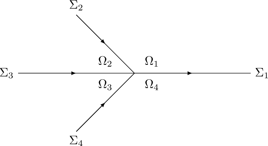
The Painlevé XXXIV parametrix satisfies the following RH problem.
RH problem 23. Find a \(2\times 2\) matrix valued function \(M^{P_{34}}(\zeta):=M^{P_{34}}(\zeta; b, \omega, s)\) with the following properties:
\(M^{P_{34}}(\zeta)\) is analytic in \(\mathbb{C} \setminus \{\cup_{j=1}^4\Sigma_j\cup\{0\}\}\), where \[\begin{align} \Sigma_1=\mathbb{R}^+, ~~ \Sigma_2=\mathrm{e}^{\frac{2 \pi \mathrm{i}}{3}}\mathbb{R}^+, ~~\Sigma_3=\mathrm{e}^{ \pi \mathrm{i}}\mathbb{R}^+,~~\Sigma_4=\mathrm{e}^{-\frac{2 \pi \mathrm{i}}{3}}\mathbb{R}^+ \end{align}\] with the orientations as shown in Figure 15.
\(M^{P_{34}}(\zeta)\) satisfies the jump condition \[\label{eq:Psi-jump} M^{P_{34}}_+ (\zeta)=M^{P_{34}}_- (\zeta) \left\{ \begin{array}{ll} \begin{pmatrix} 1 & \omega \\ 0 & 1 \end{pmatrix}, &\quad \zeta \in {\Sigma}_1, \\[9pt] \begin{pmatrix} 1 & 0 \\ \mathrm{e}^{2b\pi \mathrm{i}} & 1 \end{pmatrix}, &\quad \zeta \in {\Sigma}_2, \\[9pt] \begin{pmatrix} 0 & 1 \\ -1 & 0 \end{pmatrix},& \quad \zeta \in {\Sigma}_3, \\[9pt] \begin{pmatrix} 1 & 0 \\ \mathrm{e}^{-2b\pi \mathrm{i}} & 1 \end{pmatrix}, & \quad \zeta \in \Sigma_4. \end{array} \right .\qquad{(33)}\]
As \(\zeta \to \infty\), there exists a function \(a(s):=a(s;b,\omega)\) such that \[\begin{align} \label{eq:Psi-infinity} M^{P_{34}}(\zeta) = \begin{pmatrix} 1 & 0\\ -\mathrm{i}a(s) & 1 \end{pmatrix} \left(I+\frac{M^{P_{34}}_1(s)}{\zeta} +\mathcal{O} \left( \zeta^{-2} \right) \right) \frac{\zeta^{-\frac{1}{4}\sigma_3}}{\sqrt{2}} \begin{pmatrix} 1 & \mathrm{i} \\ \mathrm{i}& 1 \end{pmatrix} \mathrm{e}^{-(\frac{2}{3}\zeta^{\frac{3}{2}}+s\zeta^{\frac{1}{2}}) \sigma_3}, \end{align}\qquad{(34)}\] where we take the principle branch for the fractions and \[\begin{align} \left(M^{P_{34}}_1(s)\right)_{12}&=\mathrm{i}2^{-\frac{2}{3}}(H-q)(-2^{\frac{1}{3}}s):=\mathrm{i}a(s),\label{p34entry-1}\\ \left(M^{P_{34}}_1(s)\right)_{11}&=2^{-\frac{7}{3}}(H^2-q^2)(-2^{\frac{1}{3}}s)-2^{-\frac{4}{3}}(q_s+qH)(-2^{\frac{1}{3}}s),\label{p34entry-2}\\ \left(M^{P_{34}}_1(s)\right)_{22}&=2^{-\frac{7}{3}}(H^2-q^2)(-2^{\frac{1}{3}}s)+2^{-\frac{4}{3}}(q_s+qH)(-2^{\frac{1}{3}}s),\label{p34entry-3} \end{align}\] {#eq: sublabel=eq:p34entry-1,eq:p34entry-2,eq:p34entry-3} with \(q(s)\) is the generalized Hastings-Mcleod solution of the Painlevé II equation \[\label{painleve2} q''(s)=sq(s)+2q^3-\nu,\quad \nu=2b+\frac{1}{2},\qquad{(35)}\] which is characterized by the following asymptotics \[q(s)=\begin{cases} \frac{\nu}{s}+\mathcal{O}(s^{-4}), &s\to+\infty,\\ \sqrt{-\frac{s}{2}}+\mathcal{O}(s^{-1}), &s\to-\infty. \end{cases}\] \(H(s)\) is the Hamiltonian for Painlevé II equation \[\label{hamil32for32p2} H(s)=\left(q'(s)\right)^2-sq^2(s)-q^4(s)+2\nu q(s),\quad H'(s)=-q^2.\qquad{(36)}\]
As \(\zeta \to 0\), we have, if \(-\frac{1}{2} < b < 0\), \[M^{P_{34}}(\zeta)=\mathcal{O} \left( \zeta^{b} \right) ,\] and if \(b \geq 0\), \[M^{P_{34}}(\zeta)=\left\{ \begin{array}{ll} \begin{pmatrix} \mathcal{O} \left( \zeta^{b} \right) & \mathcal{O} \left( \zeta^{-b} \right) \\ \mathcal{O} \left( \zeta^{b} \right) & \mathcal{O} \left( \zeta^{-b} \right) \end{pmatrix}, &\quad \zeta \in \Omega_1\cup\Omega_4, \\ \mathcal{O} \left( \zeta^{-b} \right) , &\quad \zeta \in \Omega_2\cup\Omega_3, \end{array} \right .\] where the domains \(\Omega_j\), \(j=1,2,3,4\) are shown in Figure 15.
By [39], [54], the above RH problem is uniquely solvable for \(b>-\frac{1}{2}\), \(\omega \in \mathbb{C}\setminus (-\infty,0)\), and \(s\in \mathbb{R}\). Moreover, with \(a(s)\) given in ?? , the function \[u(s)=u(s;b,\omega):=a'(s;b,\omega)-\frac{s}{2}\] satisfies the Painlevé XXXIV equation \[\label{Bp34} u''(s)=4u(s)^2+2su(s)+\frac{u'(s)^2-(2b)^2}{2u(s)}.\tag{101}\] Particularly, one has \[u(s;b, 0)=\left\{ \begin{array}{ll} \frac{b}{\sqrt{s}}+\mathcal{O} \left( s^{-2} \right) , &\qquad s\to +\infty, \\ -\frac{s}{2}+\mathcal{O} \left( s^{-2} \right) , &\qquad s\to -\infty. \end{array}\right .\] This, together with the fact that \(a(s;b,0)\to 0\) as \(s\to -\infty\), implies that \[\label{equ:def32of32a40s41} a(s;b,0)=\int_{-\infty}^s \left( u(z;b, 0) + \frac{z}{2}\right) \mathop{}\!\mathrm{d}z.\tag{102}\]
In this paper, we focus on the special case where \(b=0\), which by ?? implies that \(\nu=1/2\). It can be inferred from [39] that \(q(s)\) has a special solution which can be constructed through Airy function as \[\label{equ:spe32p2} q(s)=-2^{-\frac{1}{3}}\frac{\mathrm{Ai} '(-2^{-\frac{1}{3}}s)}{\mathrm{Ai} (-2^{-\frac{1}{3}}s)}.\tag{103}\] Indeed, from the asymptotics of Airy functions, it follows that \[q(s)\sim\frac{1}{2}\sqrt{2}(-s)^{\frac{1}{2}},\quad s\to-\infty.\] Take the formula 103 into \(H(s)\) in ?? , along with the properties of Airy function(\(\mathrm{Ai}'' (s)=s\mathrm{Ai} (s)\)), we have \[\begin{align} \left(M^{P_{34}}_1(s)\right)_{12}&= \frac{s^2\mathrm{i}}{4},\tag{104}\\ \left(M^{P_{34}}_1(s)\right)_{11}&=\frac{s^4}{32}-\frac{s}{4},\tag{105}\\ \left(M^{P_{34}}_1(s)\right)_{22}&=-\frac{s^2}{4}\frac{\mathrm{Ai} '(s)}{\mathrm{Ai} (s)}+\frac{s^4}{32}+\frac{s}{4}.\tag{106} \end{align}\]
7 The proof of Proposition 16↩︎
To prove Proposition 16, we need several Lemmas as follows.
Lemma 6. For \(0<a<1<b\), denote \(I(a,b)=\int_{-b}^{-a}\frac{|p^2-1||p+1|}{|p^2-a^2|^{1/2}|p^2-b^2|^{1/2}}\mathop{}\!\mathrm{d}p\), then we have \[\label{equ:Id} I(a,b) = \frac{1}{b}K(u)-bE(u),\qquad{(37)}\] where \(u = \sqrt{1 -\frac{a^2}{b^2}}\), and the complete elliptic integrals \(K(u)\) and \(E(u)\) are defined by \[\begin{align} \label{def:EuKu} K(u) = \int_0^{\pi/2}\frac{1}{\sqrt{1-u^2\sin^2\theta}}\mathop{}\!\mathrm{d}\theta,\quad E(u) = \int_0^{\pi/2}\sqrt{1-u^2\sin^2\theta}\mathop{}\!\mathrm{d}\theta. \end{align}\qquad{(38)}\]
Proof. For \(0<a<1<b\), by substituting \(p\to-p\), the integral \(I(a,b)\) can be simplified as \[I(a,b)=\int_a^b\frac{(p+1)(p-1)^2}{\sqrt{p^2-a^2}\,\sqrt{b^2-u^2}}\mathop{}\!\mathrm{d}p.\] Now introduce the following trigonometric substitution \[v = \sqrt{a^2\sin^2\varphi+b^2\cos^2\varphi},\quad \varphi\in[0,\pi/2],\] we have \[\begin{align} &u^2-a^2 = (b^2-a^2)\cos^2\varphi,\quad b^2-u^2 = (b^2-a^2)\sin^2\varphi,\\ &\frac{\mathop{}\!\mathrm{d}v}{\mathop{}\!\mathrm{d}\varphi } = -\frac{(b^2-a^2)\sin\varphi\cos\varphi}{v}. \end{align}\] By the above substitution, \(I(a,b)\) can be reduced to \[\label{equ:reduction32of32I} I(a,b) = \int_0^{\pi/2} \frac{(v+1)(v-1)^2}{v}\mathop{}\!\mathrm{d}\varphi= \int_0^{\pi/2}\frac{\mathop{}\!\mathrm{d}\varphi}{v} - \int_0^{\pi/2}v\mathop{}\!\mathrm{d}\varphi.\tag{107}\] It can be deduced from \(u^2 = 1-\frac{a^2}{b^2}\) that \(v = b\sqrt{1-k^2\sin^2\varphi}\), which brings up \[\label{equ:intv} \begin{align} &\int_0^{\pi/2} v\mathop{}\!\mathrm{d}\varphi = b\int_0^{\pi/2}\sqrt{1-u^2\sin^2\varphi}\mathop{}\!\mathrm{d}\varphi = bE(u),\\ &\int_0^{\pi/2}\frac{\mathop{}\!\mathrm{d}\varphi}{v} = \frac{1}{b}\int_0^{\pi/2}\frac{\mathop{}\!\mathrm{d}\varphi}{\sqrt{1-u^2\sin^2\varphi}} = \frac{1}{b}K(u), \end{align}\tag{108}\] where \(K(u)\) and \(E(u)\) are defined as in ?? . Formula ?? can be proved by the results in 107 and 108 . ◻
Lemma 7. The function \(I(a,\cdot):(1, \sqrt{2}) \to \mathbb{R}\) defined in ?? is strictly increasing as to variable \(b\) with fixed \(0<a<1\). Moreover, As \(a\to0\), \(I(a,b)\) has the following asymptotics: \[I(a,b) =\frac{1}{\sqrt{2}}\log\frac{1}{a}+\frac{\log 4\sqrt{2}-1}{\sqrt{2}}+\mathcal{O}\left(a^2\log a\right),\quad a\to0,\] and in particular \(I(a,b)\sim\frac{1}{\sqrt{2}}\log\frac{1}{a}\).
Proof. We differentiate the closed-form expression in ?? with respect to \(b\). From \(u = \sqrt{1 -\frac{a^2}{b^2}}=\sqrt{2 -\frac{2}{b^2}}\), one computes \[\label{equ:dif32u} \frac{\mathop{}\!\mathrm{d}u}{\mathop{}\!\mathrm{d}d} = \frac{\sqrt{2}}{b^2\sqrt{b^2-1}}.\tag{109}\] Using the classical differentiation formulas for the complete elliptic integrals, we have \[\frac{\mathop{}\!\mathrm{d}E}{\mathop{}\!\mathrm{d}u} = \frac{E(u)-K(u)}{u}, \quad \frac{\mathop{}\!\mathrm{d}K}{\mathop{}\!\mathrm{d}u} = \frac{E(u)-(1-u^2)K(u)}{u(1-u^2)}.\] Together with 109 , the chain rule yields \[\label{equ:dE47dd} \frac{\mathop{}\!\mathrm{d}E}{\mathop{}\!\mathrm{d}b} = \frac{E(u)-K(u)}{b(b^2-1)}, \qquad \frac{\mathop{}\!\mathrm{d}K}{\mathop{}\!\mathrm{d}b} = \frac{b^2E(u) - a^2K(u)}{a^2b(b^2-1)}.\tag{110}\] From equation 110 , we obtain \[\begin{align} \frac{\mathop{}\!\mathrm{d}}{\mathop{}\!\mathrm{d}b}\bigl[bE(u)\bigr] = E(u) + \frac{E(u)-K(u)}{b^2-1}, \quad \frac{\mathop{}\!\mathrm{d}}{\mathop{}\!\mathrm{d}b}\left[\frac{K(u)}{b}\right] = \frac{E(u)-a^2K(u)}{a^2(b^2-1)}, \end{align}\] which implies that for \(0<a<1\), \[\frac{\mathop{}\!\mathrm{d}I(a,b)}{\mathop{}\!\mathrm{d}b}=\frac{(1-a^2b^2)E(u)}{a^2(b^2-1)}>0.\] Therefor, \(I(a,b)\) is strictly increasing as to variable \(b\).
It remains to prove the asymptotic behavior of \(I(a,b)\) as \(a\to0^+\), \(b\to\sqrt{2}^-\). As \(a\to0^+\), we have \(u\to 1^-\), with complementary modulus \(u^\prime =\sqrt{1-u^2}= \frac{a}{b}\to 0^+\). Applying the asymptotics of elliptic integrals given in formula 17.3.26 of [55], we obtain the following asymptotics of \(K(u)\) and \(E(u)\) as \(u\to 1^-\): \[\begin{align} K(u) &= \log\frac{4}{u^\prime} + \mathcal{O}\left((u^\prime)^2\log\tfrac{1}{u^\prime}\right) = \log\frac{4\sqrt{2}}{a} + \mathcal{O}\left(a^2\log a\right), \tag{111} \\ E(u) &= 1 + \mathcal{O}\left((u^\prime)^2\log\frac{1}{u^\prime}\right) = 1 +\mathcal{O}\left(a^2\log a\right). \tag{112} \end{align}\] Substituting 111 –112 into ?? , we obtain \[\begin{align} I(a,b)= \frac{1}{\sqrt{2}}\log\frac{1}{a}+\frac{\log 4\sqrt{2}-1}{\sqrt{2}}+\mathcal{O}\left(a^2\log a\right), \quad a\to0. \end{align}\] ◻
Now, with the help of Lemma 6 and Lemma 7, we finish the proof of Proposition 16.
Proof. (Proposition 16) Recalling the notation of Lemma 6, equation ?? reads \[(E_1 - k_0)^{\frac{1}{2}}\mathrm{e}^{8\tau I(a,b)} = 1.\] Taking the natural logarithm transforms this into the following equivalent condition \[\label{eq:Id95equiv} I(a,b) =- \frac{\log(E_1-k_0)}{16\tau}.\tag{113}\] From the definition of \(\tau\) in 77 we have \[E_1-k_0=\frac{\xi-4(\alpha+\beta)}{4}=\frac{1}{\sqrt{2}}\left(\frac{\tau}{t}\right)^{\frac{1}{2}}.\] From \(I(a,b)\sim\frac{1}{\sqrt{2}}\log\frac{1}{a}\) proved in Lemma 7, we have \[0<I(a,b)\lesssim\frac{1}{\sqrt{2}}\log\frac{1}{a},\quad 0<a<1,\] which leads to \[\label{the32equation32of32TIII} C<\sqrt{\frac{t}{\log t}}\left[\xi-4(\alpha+\beta)\right]<2^{-\frac{3}{4}}\tag{114}\] for any \(0<C<2^{-3/4}\), which is exactly the region \(\mathcal{T}_{\mathrm{\uppercase{\romannumeral3}}}\) we consider.
From Lemma 6 and Lemma 7, We know that function \(I(a,\cdot):(1,\sqrt{2})\to(0,+\infty)\) is a continuous, strictly increasing bijection. For every \(t>0\), right hand of the formula 113 lies in this range. The intermediate value theorem provides at least one solution for \(1<b<\sqrt{2}\) to 113 , and strict monotonicity guarantees it is unique. ◻
Acknowledgements↩︎
This work is supported by the National Natural Science Foundation of China (Grant No. 12271104).