Incremental Tensor-Train Compression from Streaming TT-Formatted Data: Applications to Reduced-Order Modeling
June 25, 2026
Abstract
High-dimensional tensor data streams arise naturally in scientific and engineering applications, such as simulations of kinetic equations and quantum systems, where samples become available sequentially and are often already represented in compressed low-rank tensor formats. Existing streaming tensor-train (TT) algorithms typically construct or update representations from dense tensor data or randomized sketches. However, when high-dimensional data are generated directly in TT or related low-rank formats, reconstructing dense tensors solely for the purpose of compression is unnecessary and computationally prohibitive. We develop a deterministic incremental TT compression algorithm that operates directly on streaming TT-formatted data. Given a new TT tensor, the proposed method updates an accumulated TT representation through core-wise projection, residual orthogonalization, and adaptive enrichment, retaining only the complementary information that cannot be represented within a prescribed tolerance. By operating entirely at the level of TT cores, the algorithm avoids reconstructing either the incoming tensor or the accumulated full tensor. We establish approximation error bounds for the proposed incremental approach. Moreover, we show that the accumulated TT representation corresponds to a compressed analogue of standard proper orthogonal decomposition for full-order snapshot data, enabling reduced-order models to be constructed directly from streaming low-rank solution data through operations on TT cores, without first reconstructing full snapshots. Numerical experiments on parametric radiative transfer equations demonstrate that the proposed method achieves comparable reconstruction accuracy with substantially reduced wall time and yields efficient and accurate ROMs directly from compressed low-rank data.
1 Introduction↩︎
High-dimensional tensor data streams arise naturally in many areas of scientific computing, including uncertainty quantification, machine learning, optimal control, and simulations of high-dimensional PDEs arising from statistical or quantum physics. In these settings, data often become available sequentially, and each sample may itself be a high-dimensional tensor, as occurs, for example, in repeated solves of high-dimensional parametric partial differential equations (PDEs) [1]–[4]. Directly storing and processing the accumulated data quickly becomes infeasible because the number of degrees of freedom (DOFs) grows exponentially with the tensor dimension, a phenomenon commonly referred to as the curse of dimensionality. Consequently, efficient algorithms must compress and process streaming tensor data without explicitly forming the full accumulated tensor.
Tensor decompositions provide a natural and powerful framework for addressing this challenge. Among them, the tensor-train (TT) format is particularly attractive because it provides stable, quasi-optimal truncation while achieving storage and computational complexities that scale linearly with the tensor dimension when the TT ranks remain moderate [5], [6]. While classical TT algorithms assume that all tensor data are available beforehand, many modern applications generate data sequentially. This has led to growing interest in streaming TT algorithms, which update compressed tensor representations as new samples become available. Streaming TT approximation (STTA) [7] constructs TT representations from randomized sketches, whereas deterministic approaches such as TT-FOA [8] and TT-ICE [9] incrementally update a TT representation as new tensor data become available.
Despite this progress, a fundamental mismatch remains: existing deterministic incremental TT algorithms assume that incoming data are accessed through dense tensor entries. In many modern scientific computing applications, however, it is common and preferable to compute and store high-dimensional solutions directly in compressed form rather than as dense tensors. For instance, in multi-query tasks involving high-dimensional PDEs, such as kinetic equations and quantum systems, low-rank solvers compute solution tensors directly in TT or related low-rank tensor formats [3], [4], [10], [11]. In such settings, reconstructing dense tensors solely for streaming compression incurs exponential storage overhead and negates the computational advantage of the low-rank solver.
In addition, a similar mismatch arises in reduced-order modeling for these high-dimensional PDEs. Classical ROMs [2] are constructed from full-order solution data. Recent tensor-based ROMs [12]–[17] further introduce tensor compression or tensorial operations into the ROM construction, but their construction still relies on full-order data. Although tensor-based dynamic mode decomposition [18] can handle time-history data in TT format, it does not consider the streaming setting in which each solution snapshot arrives sequentially in low-rank form. Hence, existing methods do not directly leverage streaming solution data generated by low-rank solvers in compressed low-rank form.
In this work, we address these bottlenecks by developing a deterministic incremental TT compression algorithm that operates directly on streaming TT-formatted data. Given a new TT tensor, the proposed method updates an accumulated TT representation through core-wise projection, residual orthogonalization, and adaptive enrichment. At each mode, the incoming TT core is projected onto the current TT subspace, and only information that cannot be represented within a prescribed tolerance is retained. As a result, the algorithm operates entirely on TT cores and avoids reconstructing either the incoming tensor or the full accumulated tensor. Beyond data compression, we show that the accumulated TT tensor can be interpreted as a decomposition into a compressed reduced basis and training-sample coefficients, enabling efficient model order reduction directly from low-rank data.
The main contributions of this work are summarized as follows:
Incremental TT construction from streaming TT-formatted data. We propose a deterministic algorithm that incrementally constructs an accumulated TT representation directly from TT-formatted inputs without reconstructing dense tensors.
Core-wise project-and-enrich update strategy. The proposed method performs projection, residual orthogonalization, and adaptive enrichment directly on TT cores, enabling rank-adaptive updates while maintaining a prescribed approximation accuracy.
Theoretical guarantees. We establish approximation error bounds showing that, in the absence of truncation, the reconstruction error for each processed tensor is bounded by \(\sqrt{d}\epsilon\). We also derive complexity estimates showing that the computational cost scales linearly with the tensor dimension.
Application to reduced-order modeling. We show that the accumulated TT representation provides a compression of solution data analogous to proper orthogonal decomposition (POD), thereby enabling efficient low-rank ROMs that are directly compatible with modern low-rank solvers.
Numerical experiments on parametric radiative transfer equations (RTEs) demonstrate the accuracy, efficiency, and scalability of the proposed method and its application to ROM.
The remainder of the paper is organized as follows. Section 2 reviews background material on tensor-train representations. Section 3 presents the incremental TT compression algorithm. Section 4 establishes the approximation properties and computational complexity. Section 5 develops reduced-order modeling formulations based on the accumulated TT representation. Section 6 reports numerical experiments, and Section 7 concludes the paper.
2 Tensor train decomposition↩︎
The TT decomposition is an efficient low-rank representation for high-dimensional tensors, effectively mitigating the curse of dimensionality. Given a \(d\)-dimensional tensor \(\boldsymbol{A} \in \mathbb{R}^{n_1 \times n_2 \times \cdots \times n_d}\), the TT format represents \(\boldsymbol{A}\) as a sequence of third-order tensors (TT cores) through a matrix product structure \[\label{eq:tt} \boldsymbol{A}(i_1,\dots,i_d) = \mathcal{V}_1(1,i_1,:) \, \mathcal{V}_2(:,i_2,:) \cdots \mathcal{V}_d(:,i_d,1),\tag{1}\] where each core \(\mathcal{V}_i \in \mathbb{R}^{r_{i-1} \times n_i \times r_i}\), and \(\{r_i\}_{i=0}^d\) are the TT ranks with \(r_0 = r_d = 1\). The TT ranks quantify the coupling between adjacent modes and determine both the approximation accuracy and the computational cost. For brevity, we may suppress the indices in 1 and write \(\boldsymbol{A} = \mathcal{V}_1\,\mathcal{V}_2 \cdots \mathcal{V}_d.\)
The storage complexity of the TT representation is \(O\!\left(\sum_{i=1}^d n_i r_{i-1} r_i\right),\) which, under the assumption \(n_i \sim n\) and \(r_i \sim r\), scales as \(O(d n r^2)\). This linear scaling in the dimension \(d\) contrasts sharply with the exponential complexity \(O(n^d)\) required to store the full tensor.
Given a full tensor \(\boldsymbol{B}\in\mathbb{R}^{n_1 \times n_2 \times \cdots \times n_d}\), the standard construction of its TT decomposition \(\boldsymbol{A}\) is the
TT-SVD algorithm [5], which relies on successive tensor unfoldings (also called matricizations) and truncated SVDs. The
mode-\(i\) unfolding reshapes \(\boldsymbol{B}\) into a matrix, denoted by \[B_{\langle i \rangle}=\texttt{reshape}(\boldsymbol{B},[n_1\cdots n_i, \;n_{i+1}\cdots
n_{d}]) \in \mathbb{R}^{(n_1\cdots n_i) \times (n_{i+1} \cdots n_d)}.\] Moreover, a tensor is uniquely determined by any of its unfoldings; that is, two tensors are identical if and only if their mode-\(i\)
unfoldings coincide. Applying a truncated SVD to the first unfolding, \(B_{\langle 1 \rangle} \approx U_1 S_1 V_1^\top,\) yields a rank-\(r_1\) approximation with error bounded by \(\epsilon_1\) in the Frobenius norm. The first core \(\mathcal{V}_1\) of \(\boldsymbol{A}\) is obtained by reshaping \(U_1\in\mathbb{R}^{n_1\times r_1}\) into a tensor of size \(1\times n_1\times r_1\). The remaining factor \(S_1V_1^\top\in\mathbb{R}^{r_1\times(n_2\cdots n_d)}\)
is interpreted as a tensor of size \(r_1\times n_2\times\cdots\times n_d\). Grouping the first two indices gives a matrix \(C_2\in\mathbb{R}^{(r_1n_2)\times(n_3\cdots n_d)},\) to which the
next truncated SVD with rank \(r_2\) and approximation error \(\epsilon_2\), \(C_2\approx U_2S_2V_2^\top,\) is applied. The second core \(\mathcal{V}_2\) is then obtained by reshaping \(U_2\in\mathbb{R}^{r_1n_2\times r_2}\) into a tensor of size \(r_1\times n_2\times r_2\). Repeating this
procedure, at the \(i\)-th step, a truncated SVD produces factors \(U_i S_i V_i^\top\) with approximation error \(\epsilon_i\), from which the core \(\mathcal{V}_i \in \mathbb{R}^{r_{i-1} \times n_i \times r_i}\) is obtained by reshaping \(U_i\in\mathbb{R}^{r_{i-1}n_i\times r_i}\). This process continues until all cores are constructed. The
computational complexity of TT-SVD is dominated by the SVDs of the unfolding matrices and scales as \(O\!\left(\sum_{i=1}^{d-1} r_{i-1} n^{\,d-i+1}\right),\) assuming \(n_i \sim
n\). The resulting approximation is quasi-optimal in the sense that the error is within a small constant factor of the best achievable TT approximation with the same ranks, with error bounded by \(\|\boldsymbol{B} -
\boldsymbol{A}\|_F \;\le\; \sqrt{\sum_{i=1}^{d-1} \epsilon_i^2}.\)
If a tensor is already given in TT format, it can be recompressed using the TT-rounding algorithm with a prescribed threshold \(\epsilon_{\rm tt}\). This procedure consists of successive orthogonalizations
(via QR factorizations) and truncated SVDs applied to matricizations of the TT cores, producing a compressed TT representation with reduced ranks. The resulting approximation is quasi-optimal, as TT-rounding is mathematically equivalent to
TT-SVD applied to the full tensor. The computational complexity of TT-rounding scales as \(O(d n r^3)\), thereby avoiding the exponential scaling with respect to \(d\).
3 Incremental construction of TT reduced basis from low-rank data↩︎
Consider a sequence of low-rank data \(\{\boldsymbol{A}^k\}_{k=1}^{n_\mu}\), where each tensor \(\boldsymbol{A}^k \in \mathbb{R}^{n_1\times\cdots\times n_d}\) is already available in the TT format 1 . Specifically, each \(\boldsymbol{A}^k\) is characterized by TT cores \(\mathcal{V}_i^k \in \mathbb{R}^{s_{i-1}\times n_i \times s_i}\) with TT ranks \(\{s_i\}_{i=0}^d\) satisfying \(s_0 = s_d = 1\). The proposed incremental algorithm progressively constructs a \((d+1)\)-dimensional accumulated tensor \({\boldsymbol{\psi}}\in \mathbb{R}^{n_1\times\cdots\times n_d\times n_\mu}\) in the TT format \[{\boldsymbol{\psi}}= {\mathcal{U}}_1\,{\mathcal{U}}_2\,\cdots {\mathcal{U}}_{d}\,{\mathcal{U}}_{d+1}\] with TT cores \(\{{\mathcal{U}}_i\}_{i=1}^{d+1}\) and TT ranks \(\{r_i\}_{i=0}^{d+1}\), \(r_0=r_{d+1}=1\), such that \(\| \boldsymbol{A}^k-{\boldsymbol{\psi}}(:,:,\cdots,:,k) \|_F\lesssim \epsilon\), \(k=1,\ldots,n_\mu\), where \(\epsilon\) is a prescribed error tolerance.
To initialize the algorithm, we may construct \({\boldsymbol{\psi}}^1\) directly from the first tensor \({\boldsymbol{A}}^1\) and start the incremental updates at \(k=2\). Alternatively, warm-start initialization based on prior knowledge of the dataset is also possible. Suppose that after processing the first \(k-1\) tensors, we have already constructed \({\boldsymbol{\psi}}^{k-1}\) with TT cores \(\{{\mathcal{U}}_i^{k-1}\}_{i=1}^{d+1}\) as the current TT approximation of the accumulated tensor. When a new tensor \(\boldsymbol{A}^{k}\) with cores \(\{{\mathcal{V}}^k_i\}_{i=1}^{d}\) becomes available, the TT cores of \({\boldsymbol{\psi}}^{k-1}\) are updated to produce \({\boldsymbol{\psi}}^{k}\) while maintaining the prescribed accuracy guarantee. Furthermore, we assume that each core of the accumulated TT \(\mathcal{U}_i^{k-1}\) is left-orthogonal, meaning that its left unfolding \[U_i^{k-1} := \texttt{reshape}\!\left(\mathcal{U}_i^{k-1},\,[r_{i-1}^{k-1} n_i,\; r_i^{k-1}]\right)\] has orthonormal columns. We also assume that the cores \(\{{\mathcal{V}}^k_i\}_{i=1}^{d}\) of the incoming TT tensor \(\boldsymbol{A}^{k}\) are right-orthogonal. Specifically, for each \(i\), the right unfolding \[V^k_i := \texttt{reshape}\!\left(\mathcal{V}^k_i,\,[s_{i-1},\; n_i s_i]\right),\] has orthonormal rows.
(a) Processing the first mode.
Define \(\mathcal{W}_1 := \mathcal{V}_1^{k}\) and \[W_1 := \texttt{reshape}\!\left(\mathcal{W}_1,\,[n_1,\, s_1]\right).\] We project \(W_1\) onto the orthogonal complement of the column space of \(U_1^{k-1}\) and define the residual in mode-1 \[R_1 = \big(I - U_1^{k-1} (U_1^{k-1})^T\big) W_1,\] which represents the component of the new tensor not captured by the current TT subspace. Applying a QR decomposition yields \[P_1 = \texttt{orth}(R_1),\] whose columns form an orthonormal basis for \(\mathrm{range}(R_1)\). By construction, \[\big(U_1^{k-1} (U_1^{k-1})^T + P_1P_1^T\big) W_1 = W_1. \label{eq:projection951}\tag{2}\]
(b) Updating \({\mathcal{U}}^{k-1}_i\rightarrow{\mathcal{U}}^{k}_{i}\) and processing the next mode.
For \(i=1\), no padding is required, and we set \(\widetilde{{\mathcal{U}}}^{k-1}_1={\mathcal{U}}^{k-1}_1\) and \(\widetilde{U}^{k-1}_1=U^{k-1}_1\). For \(i>1\), as noted in [9], [19], the rank change in the previous TT core update for \({\mathcal{U}}_{i-1}^{k}\) requires a zero-padding procedure for the current core \({\mathcal{U}}^{k-1}_i\) to restore dimension consistency of the TT representation. This procedure yields the padded core \(\widetilde{{\mathcal{U}}}^{k-1}_i\) of size \(r_{i-1}^{k}\times n_i\times r_i^{k-1}\) and the associated left unfolding \(\widetilde{U}^{k-1}_i\). The padded core preserves the left-orthogonality of \({\mathcal{U}}^{k-1}_i\).
If the residual satisfies \(\|R_i\|_F > \epsilon\), the mode-\(i\) component of \(\boldsymbol{A}^k\) contains significant new information and should be incorporated into the accumulated subspace \(\mathrm{range}(\widetilde{U}_i^{k-1})\). In this case, the increment \(P_i\) is appended to \(\widetilde{U}_i^{k-1}\), yielding \[\label{eq:Uupdate} U_i^{k} = \big[\widetilde{U}_i^{k-1} \;\; P_i\big],\tag{3}\] whose columns remain orthonormal. This construction satisfies an exactness property (see Lemma 1). The rank is updated as \(r_i^{k} = r_i^{k-1} + p_i\), where \(p_i \le s_i\) is the number of columns of \(P_i\). Otherwise, the new information is already well represented by \(\widetilde{U}_i^{k-1}\) up to the prescribed tolerance, and no enrichment is performed. We set \(U_i^{k} = \widetilde{U}_i^{k-1}\) with \(r_i^{k} = r_i^{k-1}\), yielding a controlled approximation error bound (see Lemma 2). The updated core is obtained by reshaping \[\mathcal{U}_i^{k} = \texttt{reshape}\!\left(U_i^{k},\,[r_{i-1}^{k},\, n_i,\, r_i^{k}]\right).\]
If \(i < d\), we proceed to the next mode and compute \[\label{eq:W} \mathcal{W}_{i+1} := \texttt{reshape}\!\left((U_i^{k})^T W_i V^k_{i+1},\,[r_i^{k},\, n_{i+1},\, s_{i+1}]\right),\tag{4}\] and its left unfolding \(W_{i+1} := \texttt{reshape}\!\left(\mathcal{W}_{i+1},\,[r_i^{k} n_{i+1},\, s_{i+1}]\right).\) The residual with respect to the padded matrix \(\widetilde{U}_{i+1}^{k-1}\) is defined as: \[R_{i+1} = \big(I - \widetilde{U}_{i+1}^{k-1} (\widetilde{U}_{i+1}^{k-1})^T\big) W_{i+1}.\] Applying a QR decomposition yields an orthonormal increment \[P_{i+1} = \texttt{orth}(R_{i+1}),\] ensuring the decomposition holds: \[\big(\widetilde{U}_{i+1}^{k-1} (\widetilde{U}_{i+1}^{k-1})^T + P_{i+1} P_{i+1}^T\big) W_{i+1} = W_{i+1}. \label{eq:projection95i95p1}\tag{5}\] The mode-one projection identity 2 is the special case of 5 obtained from \(\widetilde{U}^{k-1}_{1}=U^{k-1}_1\).
(c) Updating the last core.
The update of the last core is slightly different. The matrix \(W_d\) is projected onto the column space of \(U_d^{k}\), yielding the slice \[W_{d+1} = (U_d^{k})^T W_d \in \mathbb{R}^{r_d^{k} \times 1}.\] Applying the zero-padding procedure to the last core \(\mathcal{U}_{d+1}^{k-1}\) produces the padded core \(\widetilde{\mathcal{U}}_{d+1}^{k-1}\in\mathbb{R}^{r_d^k\times (k-1)\times 1}\). We then append \(W_{d+1}\) as the \(k\)-th slice to form the updated core \(\mathcal{U}_{d+1}^k \in \mathbb{R}^{r_d^k \times k \times 1}\): \[\mathcal{U}_{d+1}^{k}(:, 1:k-1, 1) = \widetilde{\mathcal{U}}_{d+1}^{k-1}, \quad \mathcal{U}_{d+1}^{k}(:, k, 1) = W_{d+1}.\] Consequently, the updated accumulated tensor is given by \[{\boldsymbol{\psi}}^{k} = {\mathcal{U}}^{k}_1{\mathcal{U}}^{k}_2\cdots {\mathcal{U}}^{k}_{d}\,{\mathcal{U}}^{k}_{d+1}.\]
(d) Re-orthogonalization and truncation for rank control.
If the TT ranks of \({\boldsymbol{\psi}}^{k}\) exceed a prescribed maximum \(r_{\mathrm{max}}\), TT-rounding is performed to reorthogonalize the TT cores, remove redundant
information, and reduce the TT ranks of \({\boldsymbol{\psi}}^{k}\) while maintaining the prescribed accuracy.
The proposed construction employs an incremental project-and-enrich strategy to build the reduced basis and, unlike existing approaches [15], avoids the exponential scaling with the dimension. The overall procedure is summarized in Algorithm 1.
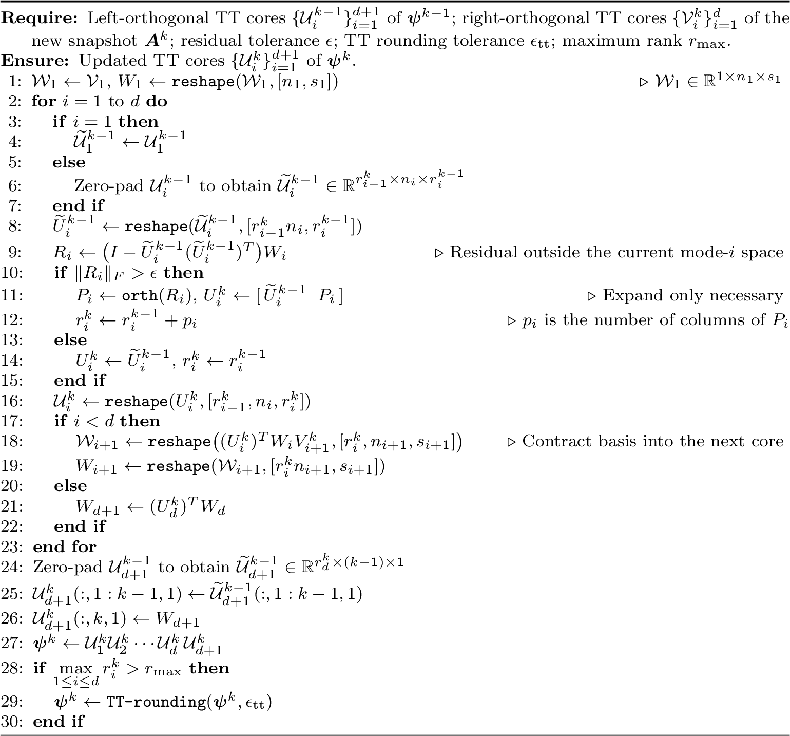
Comparison with existing incremental TT algorithms. The proposed method is related to deterministic streaming TT algorithms such as TT-FOA [8] and TT-ICE [9]. Unlike these methods, however, it targets streaming low-rank data already represented in TT form. TT-FOA tracks a fixed-rank TT model of the accumulated data tensor by recursively updating the cores through a weighted least-squares fit. TT-ICE is closer in spirit to our method, as both methods adaptively expand the TT cores of an accumulated tensor by appending orthogonal directions needed to represent new tensors. The key distinction lies in how the streaming data are represented. TT-FOA uses dense or sampled tensor entries, while TT-ICE assumes access to dense tensor data and forms residuals from their unfoldings. In contrast, the proposed approach takes each incoming tensor directly in TT form and propagates compressed interfaces through a sweep. Thus the projection, residual enrichment, and coefficient update are performed at the TT-core level, without materializing or densely unfolding the incoming tensor. This distinction is essential for data generated by emerging low-rank solvers, where reconstructing dense snapshots would negate the computational advantage of the low-rank representation.
4 Theoretical properties↩︎
In this section, we establish the approximation property for the proposed incremental low-rank TT algorithm. We begin with an exactness property of the core-wise entrichment for our construction.
Lemma 1 (Exactness of the core-wise enrichment). The Algorithm 1 generates implicitly a sequence of intermediate TT tensors \[\begin{align} &\boldsymbol{A}^{k}_{0} = \boldsymbol{A}^{k},\\ &\boldsymbol{A}^{k}_{i} = {\mathcal{U}}^{k}_1\cdots {\mathcal{U}}^{k}_{i}\,\mathcal{W}_{i+1}\,{\mathcal{V}}^k_{i+2}\cdots{\mathcal{V}}^k_{d},\quad i=1,\ldots,d-2, \\ &\boldsymbol{A}^{k}_{d-1} = {\mathcal{U}}^{k}_1\cdots {\mathcal{U}}^{k}_{d-1}\,\mathcal{W}_{d}, \\ &\boldsymbol{A}^{k}_{d} = {\mathcal{U}}^{k}_1\cdots {\mathcal{U}}^{k}_{d}\,{\mathcal{U}}^{k}_{d+1}(:,k,1)=\boldsymbol{\psi}^{k}(:,:,\cdots,:,k). \end{align}\] In addition, for each \(i=1,\dots,d\), if \(\|R_i\|_F > \epsilon\), then \[\label{eq:exact} \boldsymbol{A}^{k}_{i} = \boldsymbol{A}^{k}_{i-1}.\qquad{(1)}\]
Proof: The tensors \(\boldsymbol{A}_{i}^{k}\) are generated implicitly through the progressive update of the TT cores. To prove ?? for \(i=1,\ldots,d-1\), it suffices to show that \[\label{eq:update1} \mathcal{U}_i^{k}\,\mathcal{W}_{i+1}=\mathcal{W}_i\,\mathcal{V}^k_{i+1},\tag{6}\] since all remaining TT cores are identical on both sides.
When \(\|R_i\|_F>\epsilon\), the basis is enriched according to 3 , and by construction (see 5 ), we have \[U_i^{k}(U_i^{k})^T W_i = W_i.\] Therefore, \[\label{eq:update2} W_iV^k_{i+1}=U_i^{k}(U_i^{k})^T W_iV^k_{i+1}.\tag{7}\] By the definition of \(\mathcal{W}_{i+1}\) and its left unfolding \(W_{i+1}\) 4 , the right-hand side of 7 is precisely the matricization of \(\mathcal{U}_i^{k}\mathcal{W}_{i+1}\), whereas the left-hand side is the corresponding matricization of \(\mathcal{W}_i\mathcal{V}^k_{i+1}\). Since a tensor is uniquely determined by its matricization, 6 holds. We conclude that \(\boldsymbol{A}_i^{k}=\boldsymbol{A}_{i-1}^{k}\).
For the terminal case \(i=d\), the proof is similar but simpler, since there are no subsequent TT cores. We only need to verify that the final update preserves the tensor exactly. When \(\|R_d\|_F > \epsilon\), the enriched basis satisfies \[U_d^{k}(U_d^{k})^T W_d = W_d.\] Since the final slice is defined as \[W_{d+1} = (U_d^{k})^T W_d,\] it follows that \[U_d^{k}W_{d+1} = U_d^{k}(U_d^{k})^T W_d = W_d.\] Thus, the left unfolding of the updated \(d\)-th core contracted with the new slice \(W_{d+1}\) of the accumulated tensor \(\boldsymbol{\psi}^{k}\) precisely reconstructs \(W_d\), which is the left unfolding of the last core of \(\boldsymbol{A}^k_{d-1}\). This implies \(\boldsymbol{A}_d^{k} = \boldsymbol{A}_{d-1}^{k}\). Hence, ?? also holds for \(i=d\), completing the proof. \(\square\)
A direct consequence of Lemma 1 is that, if \(\|R_i\|_F > \epsilon\) for all \(i=1,\dots,d\), then the newly added TT tensor is represented exactly, i.e., \[\boldsymbol{\psi}^{k}(:,:,\cdots,:,k) = \boldsymbol{A}^{k}.\]
The next lemma shows that if the residual is bounded by the threshold, then the incremental construction guarantees an approximation error bound.
Lemma 2 (Error increment). If \(\|R_i\|_F\le \epsilon\), define the error increment tensor \[\boldsymbol{E}_i := \boldsymbol{A}_{i-1}^{k}-\boldsymbol{A}_{i}^{k}.\] Then \[\label{eq:error} \|\boldsymbol{E}_i\|_F\le \epsilon .\qquad{(2)}\]
Proof: For \(1\le i<d\), since no enrichment is performed when \(\|R_i\|_F\le \epsilon\), we have \[U_i^{k}=\widetilde{U}_i^{k-1},\] and thus \[R_i=\bigl(I-\widetilde{U}_i^{k-1}(\widetilde{U}_i^{k-1})^T\bigr)W_i=\bigl(I-U_i^{k}(U_i^{k})^T\bigr)W_i .\] By construction of \(W_{i+1}\), \[W_{i+1}=(U_i^{k})^T W_i V^k_{i+1},\] and hence \[U_i^{k}W_{i+1} = U_i^{k}(U_i^{k})^T W_i V^k_{i+1}.\] Therefore, \[\label{eq:localdiff} W_iV^k_{i+1} -U_i^{k}W_{i+1} = \bigl(I-U_i^{k}(U_i^{k})^T\bigr)W_iV^k_{i+1} = R_iV^k_{i+1}.\tag{8}\]
Let \(\mathcal{R}_i\in\mathbb{R}^{r_{i-1}^k \times n_i \times s_i}\) denote the tensor whose left unfolding is the matrix \(R_i\). By 8 , it follows that \[\label{eq:E} \boldsymbol{E}_i = \boldsymbol{A}_{i-1}^{k}-\boldsymbol{A}_{i}^{k} = \mathcal{U}_1^{k}\cdots \mathcal{U}_{i-1}^{k}\,\mathcal{R}_i\,\mathcal{V}^k_{i+1}\cdots \mathcal{V}^k_d.\tag{9}\]
Since \(\mathcal{U}_1^{k},\dots,\mathcal{U}_{i-1}^{k}\) are left-orthogonal and \(\mathcal{V}^k_{i+1},\dots,\mathcal{V}^k_d\) are right-orthogonal, contraction with these cores preserves the Frobenius norm. Hence \[\|\boldsymbol{E}_i\|_F = \|\mathcal{R}_i\|_F =\|R_i\|_F \le \epsilon.\]
For the terminal case \(i=d\), since no enrichment is performed when \(\|R_d\|_F \le \epsilon\), we have\[U_d^{k}=\widetilde{U}_d^{k-1},\]and thus\[R_d = \bigl(I-\widetilde{U}_d^{k-1}(\widetilde{U}_d^{k-1})^T\bigr)W_d = \bigl(I-U_d^{k}(U_d^{k})^T\bigr)W_d.\]By the definition of the final slice \(W_{d+1}\), \[W_{d+1} = (U_d^{k})^T W_d,\] and hence \[U_d^{k}W_{d+1} = U_d^{k}(U_d^{k})^T W_d.\] Therefore, the difference in the left unfolding of the \(d\)-th cores is exactly the residual:\[W_d - U_d^{k}W_{d+1} = \bigl(I-U_d^{k}(U_d^{k})^T\bigr)W_d = R_d.\]Recall that \(\boldsymbol{A}_{d-1}^{k}\) terminates with the core \(\mathcal{W}_d\), while \(\boldsymbol{A}_d^{k}\) replaces it with the contraction of \(\mathcal{U}_d^{k}\) and \(W_{d+1}\). Therefore, the error increment is given by\[\boldsymbol{E}_d = \boldsymbol{A}_{d-1}^{k} - \boldsymbol{A}_d^{k} = \mathcal{U}_1^{k}\cdots \mathcal{U}_{d-1}^{k}\,\mathcal{R}_d,\] where the residual tensor \(\mathcal{R}_d\) has the left unfolding \(R_d\). Since \(\mathcal{U}_1^{k},\dots,\mathcal{U}_{d-1}^{k}\) are left-orthogonal, we conclude \[\|\boldsymbol{E}_d\|_F = \|\mathcal{R}_d\|_F = \|R_d\|_F \le \epsilon.\] This completes the proof. \(\square\)
To obtain the error bound for the algorithm, we need another lemma.
Lemma 3 (Orthogonality of the error increments). The increments \(\{\boldsymbol{E}_i\}_{i=1}^d\) are mutually orthogonal in the Frobenius inner product: \[\label{eq:orth} \langle \boldsymbol{E}_i,\boldsymbol{E}_j\rangle_F = 0, \qquad i\neq j.\qquad{(3)}\]
The proof requires the following orthogonality propagation property of the TT decomposition.
Lemma 4 (Orthogonality propagation in TT format). Let two TT tensors share the same left-orthonormal cores in modes \(1,\dots,i-1\). If the left unfoldings of their \(i\)-th cores are orthogonal, then the two tensors are orthogonal in the Frobenius inner product.
Proof: See appendix. \(\square\)
Now we provide the proof for Lemma 3.
Proof: Without loss of generality, we consider \(1\le i<j\le d\).
If \(\|R_i\|_F > \epsilon\), then by Lemma 1 (exactness of the core-wise enrichment), \[\boldsymbol{E}_i = \boldsymbol{A}_{i-1}^{k}-\boldsymbol{A}_i^{k} = \boldsymbol{0},\] and hence \(\langle \boldsymbol{E}_i,\boldsymbol{E}_j\rangle_F=0\) holds trivially.
We therefore consider the case \(\|R_i\|_F \le \epsilon\). From 9 , the first \(i-1\) TT cores of \(\boldsymbol{E}_i\) are given by \(\mathcal{U}_1^{k},\dots,\mathcal{U}_{i-1}^{k},\) which are left-orthonormal. The \(i\)-th core is the residual tensor \(\mathcal{R}_i\) 9 , whose left unfolding \(R_i\) is orthogonal to \(U_i^{k}\), i.e., \[R_i^T U_i^{k}=0.\]
For \(\boldsymbol{E}_j\) with \(j>i\), if \(\|R_j\|_F>\epsilon\), then by Lemma 1, \(\boldsymbol{E}_j=\boldsymbol{0}\) and \(\langle \boldsymbol{E}_i,\boldsymbol{E}_j\rangle_F=0\) holds trivially. Otherwise, due to 9 , \(\boldsymbol{E}_j\) shares the same first \(i-1\) TT cores with \(\boldsymbol{E}_i\), while the \(i\)-th core is \(\mathcal{U}_i^{k}\), whose left unfolding is \(U_i^{k}\).
Then, \(R_i^TU_i^k=0\) together with Lemma 4 implies orthogonality and thus \[\langle \boldsymbol{E}_i,\boldsymbol{E}_j\rangle_F=0.\] \(\square\)
We are ready to establish the following approximation property.
Theorem 1. Let \(\boldsymbol{\psi}\) be the accumulated tensor constructed by the proposed TT algorithm from the sequential TT-formatted data \(\{\boldsymbol{A}^k\}_{k=1}^{n_\mu}\). If the truncation step (d) is not applied, then for each \(k=1,\ldots,n_\mu\), \[\|\boldsymbol{A}^k-\boldsymbol{\psi}(:,:,\cdots,:,k)\|_F \le \sqrt{d}\,\epsilon.\]
Proof: Fix \(k\in\{1,\dots,n_\mu\}\). When the truncation step (d) is not performed, the proposed algorithm preserves the previously constructed accumulated tensor while progressively updating its TT cores. In particular, \[\boldsymbol{\psi}(:,:,\cdots,:,k)=\boldsymbol{\psi}^{k}(:,:,\cdots,:,k).\] Let \(\{\boldsymbol{A}_i^{k}\}_{i=0}^d\) denote the sequence of intermediate tensors generated by the algorithm, where \[\boldsymbol{A}_0^{k}=\boldsymbol{A}^k, \qquad \boldsymbol{A}_d^{k}=\boldsymbol{\psi}(:,:,\cdots,:,k).\] Then \[\boldsymbol{A}^k-\boldsymbol{\psi}(:,:,\cdots,:,k) = \boldsymbol{A}_0^{k}-\boldsymbol{A}_d^{k} = \sum_{i=1}^d \boldsymbol{E}_i.\]
By Lemma 3, the increments \(\{\boldsymbol{E}_i\}_{i=1}^d\) are mutually orthogonal, and therefore \[\|\boldsymbol{A}^k-\boldsymbol{\psi}(:,:,\cdots,:,k)\|_F^2 = \sum_{i=1}^d \|\boldsymbol{E}_i\|_F^2.\]
Furthermore, by Lemma 1, if \(\|R_i\|_F>\epsilon\), then \(\boldsymbol{E}_i=\boldsymbol{0}\). Otherwise, \(\|\boldsymbol{E}_i\|_F \le \epsilon\) by Lemma 2. Hence, for all \(i=1,\dots,d\), we have \(\|\boldsymbol{E}_i\|_F \le \epsilon.\) It follows that \[\|\boldsymbol{A}^k-\boldsymbol{\psi}(:,:,\cdots,:,k)\|_F^2 \le \sum_{i=1}^d \epsilon^2 = d\,\epsilon^2,\] which yields \[\|\boldsymbol{A}^k-\boldsymbol{\psi}(:,:,\cdots,:,k)\|_F \le \sqrt d\,\epsilon.\]
\(\square\)
We conclude the section by providing a complexity analysis. Assume that the accumulated TT tensor \(\psi^{(k-1)}\) has maximum rank \(r\), and the \(k\)-th incoming tensor \(A^{(k)}\) has maximum rank \(s\). Assume also that the mode sizes satisfy \(n_i\le n\). During one incremental update, the enrichment at each mode can append at most \(s\) new vectors, and hence the intermediate updated TT ranks are bounded by \(\hat{r} := r+s\).
The storage of the accumulated TT tensor \(\psi^{(k)}\) is bounded by \(O(dn\hat{r}^2+k\hat{r})\), where the first term corresponds to the physical TT cores and the second term comes from the final sample core of size \(r_d^{(k)}\times k\times 1\). Thus, the method avoids any dense tensor storage and scales linearly with the tensor dimension \(d\) when the TT ranks remain moderate.
We next estimate the cost of one streaming update without intermediate truncation. At mode \(i\), since \(\widetilde{U}_i^{(k-1)}\in \mathbb{R}^{r_{i-1}^{(k)}n_i\times r_i^{(k-1)}},\) and \(W_i\in \mathbb{R}^{r_{i-1}^{(k)}n_i\times s_i},\) and \(r_{i-1}^{(k)}\le \hat{r}\), \(r_i^{(k-1)}\le r\), and \(s_i\le s\), the residual projection \(R_i=(I-\widetilde{U}_i^{(k-1)}(\widetilde{U}_i^{(k-1)})^T)W_i\) costs \(O(n_i\hat{r}r s)\), which is bounded by \(O(n\hat{r}^2 s)\). If enrichment is triggered, computing \(P_i=\texttt{orth}(R_i)\) by a QR factorization costs \(O(n_i\hat{r} s^2)\). The propagation step \(W_{i+1} = \texttt{reshape}\big((U_i^{(k)})^T W_i V_{i+1}^{(k)}\big)\) costs \(O(n_i\hat{r}^2s+n_{i+1}\hat{r} s^2)\), which is bounded by \(O(n\hat{r}^2s)\), as \(\hat{r}\ge s\). Therefore, the per-mode cost is bounded by \(O(n\hat{r}^2s)\), and summing over all modes gives \[O\left(dn\hat{r}^2s\right).\]
If intermediate TT-rounding is triggered, the additional cost is \[O\left(dn \hat{r}^3+k \hat{r}^2\right),\] where the first term corresponds to rounding the physical TT cores and the second term comes from
the final core.
Thus, for moderate TT ranks, Algorithm 3.1 scales linearly with the tensor dimension \(d\) in both storage and computational cost.
5 Model order reduction with the incremental TT reduced basis↩︎
As established, the proposed incremental algorithm produces a compressed accumulated TT representation of streaming TT-formatted data. We now show how this representation can be used for model order reduction of high-dimensional parametric PDEs, such as kinetic equations and quantum systems. In such settings, each solution snapshot may depend on several spatial, velocity, angular, or stochastic variables, and is therefore naturally represented as a high-dimensional tensor.
Recent low-rank solvers for high-dimensional PDEs exploit tensor-product structures in the governing equations and low-rank structure in the solution tensor to reduce both memory and computational costs [3], [4]. In many such solvers, the solution is computed directly in compressed low-rank matrix or TT form. Classical ROMs, however, are typically constructed from full-tensor or full-vector snapshots. Reconstructing full tensors from low-rank solution data solely for ROM construction would destroy the computational advantage of the low-rank solver. We avoid this mismatch by using the proposed incremental TT compression to build ROMs directly from streaming low-rank snapshots.
The accumulated TT tensor produced by the proposed algorithm plays a role analogous to classical compressed representations of training data, such as proper orthogonal decomposition (POD): it simultaneously encodes a compressed reduced basis and the corresponding coefficients associated with the training parameters. In this section, we first review the classical POD for full-order data and show the analogy between the accumulated TT representation and it. We then show how the resulting compressed TT reduced basis can be used to construct ROMs directly from low-rank solution data via core-level operations, in both non-intrusive and intrusive settings.
5.1 Classical proper orthogonal decomposition (POD)↩︎
Consider a parameterized full-order model \[\label{eq:classical95fom} A(\mu)u(\mu)=f(\mu), \qquad u(\mu)\in \mathbb{R}^{N},\tag{10}\] where \(\mu\in\mathcal{P}\) denotes the parameter such as configurations of material properties or boundary conditions. POD method follows an offline-online decomposition framework. In the offline stage, a reduced space is constructed by extracting low-rank structures across parameters from the training data. In the online stage, the prediction for new parameter can be made through an interpolation inside or a projection onto the reduced space constructed offline.
In the offline stage, given a prescribed error tolerance \(\epsilon\) and the snapshot matrix \[\label{eq:classical95snapshot95matrix} S = \big[ u(\mu_1),\,u(\mu_2),\,\ldots,\,u(\mu_{n_\mu}) \big] \in \mathbb{R}^{N\times n_\mu},\tag{11}\] the POD method constructs the reduced basis by the singular value decomposition: \[\label{eq:classical95pod95svd} S \approx U_{r}\Sigma_{r} V_{r}^T\quad\textrm{with}\quad \|S-U_{r}\Sigma_{r}V_{r}^T\|_F \le \epsilon.\tag{12}\] Here, the reduced dimension \(r\) is selected as \[\label{eq:classical95pod95rank} r = \min\left\{ m:\sum_{j=m+1}^{\min(N,n_\mu)}\sigma_j^2 \le \epsilon^2 \right\},\tag{13}\] where \(\{\sigma_j\}\) are the singular values of \(S\). The columns of \(U_{r}\in\mathbb{R}^{N\times r}\) form the reduced basis, while the columns of \(\Sigma_{r}V_{r}^T\in\mathbb{R}^{r\times n_{\mu}}\) provide the reduced coefficients for the training parameters. In the online stage, for a new parameter \(\mu\), a POD-based ROM seeks an approximation of the form \[\label{eq:classical95pod95expansion} u(\mu)\approx U_{r}c(\mu), \qquad c(\mu)\in\mathbb{R}^{r}.\tag{14}\] The reduced coefficients \(c(\mu)\) may be obtained non-intrusively by interpolations in the parameter space, or intrusively by projecting the governing equations onto the reduced space spanned by \(U_r\). These two approaches will be detailed after introducing the corresponding TT basis and coefficient core.
5.2 TT reduced basis and coefficient core↩︎
In the high-dimensional tensor setting, the full-order state is viewed as a tensor \[u(\mu)\in\mathbb{R}^{n_1\times n_2\times\cdots\times n_d}, \qquad N=n_1n_2\cdots n_d.\] Classical POD first vectorizes each snapshot and forms the snapshot matrix \[S=\big[\operatorname{vec}(u(\mu_1)),\ldots, \operatorname{vec}(u(\mu_{n_\mu}))\big] \in\mathbb{R}^{(n_1n_2\cdots n_d)\times n_\mu}.\] Equivalently, \(S\) is the unfolding that separates all physical DOFs from the training sample index.
For simplicity, we treat the training samples as a single additional mode indexed by \(k\); that is, the parameter sampling space is not further tensorized in the following construction. The proposed method constructs the accumulated snapshot tensor \[\label{eq:tt95snapshot95tensor95rom} \boldsymbol{\psi}(i_1,\ldots,i_d,k) \approx u(\mu_k)(i_1,\ldots,i_d), \qquad k=1,\ldots,n_\mu,\tag{15}\] directly in TT form, \[\label{eq:tt95snapshot95tensor95decomp95rom} \boldsymbol{\psi} = {\mathcal{U}}_1{\mathcal{U}}_2\cdots {\mathcal{U}}_d{\mathcal{U}}_{d+1}.\tag{16}\] Unfolding \(\boldsymbol{\psi}\) across the physical-sample interface \((i_1,\ldots,i_d)\mid k\) gives \[\label{eq:tt95physical95sample95unfolding} S_{\rm TT} = \boldsymbol{\psi}_{\langle d\rangle} \in \mathbb{R}^{(n_1n_2\cdots n_d)\times n_\mu}.\tag{17}\] This unfolding gives a POD-like factorization of the classical snapshot matrix: \[\label{eq:tt95unfolding95factorization} S\approx S_{\rm TT}=\Phi C, \quad \Phi\in\mathbb{R}^{(n_1n_2\cdots n_d)\times r_d}, \quad C\in\mathbb{R}^{r_d\times n_\mu}.\tag{18}\] Here, \(\Phi\) denotes the unfolding of compressed reduced basis represented implicitly by the first \(d\) TT cores. More precisely, its tensorization satisfies \[\label{eq:tt95basis95rom} \boldsymbol{\Phi}(i_1,\ldots,i_d,a) = {\mathcal{U}}_1(1,i_1,:)\, {\mathcal{U}}_2(:,i_2,:)\cdots {\mathcal{U}}_d(:,i_d,a), \qquad a=1,\ldots,r_d .\tag{19}\] Since the physical cores produced by the incremental construction are left-orthogonal, this basis is orthonormal, i.e. \(\Phi^T\Phi=I_{r_d}\). The coefficient matrix \(C\) is encoded by the final sample core, \[\label{eq:tt95coeff95core95rom} C(a,k)=c_a(\mu_k)={\mathcal{U}}_{d+1}(a,k,1), \qquad a=1,\ldots,r_d,\quad k=1,\ldots,n_\mu.\tag{20}\] Crucially, the unfolding is only conceptual: in practice, \(\Phi\) is never explicitly constructed as a dense matrix, but is stored and manipulated through its TT cores.
In summary, the first \(d\) physical cores defines a TT analogue of the POD basis, while \(C\) plays the role of the POD coefficient matrix \(\Sigma_r V_r^T\). In contrast to classical POD, neither the full snapshots, the full snapshot matrix, nor the dense reduced basis matrix is formed.
Remark 2. The use of a single sample index \(k\) is only for notational simplicity. If the training parameters are sampled on a tensor-product parameter grid, the sample mode may itself be decomposed into several parameter modes. In that case, the accumulated snapshot tensor has the form \[\boldsymbol{\psi}(i_1,\ldots,i_d,\ell_1,\ldots,\ell_p) \approx u(\mu_{\ell_1,\ldots,\ell_p})(i_1,\ldots,i_d),\] and the same construction applies by taking the interface between the physical modes \((i_1,\ldots,i_d)\) and the parameter/sample modes \((\ell_1,\ldots,\ell_p)\). The reduced basis is determined by the TT rank across this interface, while the remaining parameter cores encode the training coefficients in compressed form.
5.3 Non-intrusive coefficient interpolation↩︎
In the non-intrusive approach, solutions at new parameter values are predicted by interpolating or regressing the coefficient core, without requiring access to the governing operators. From 20 , the training data provide reduced coefficient vectors \[\label{eq:tt95training95coefficients} c(\mu_k)={\mathcal{U}}_{d+1}(:,k,1)\in\mathbb{R}^{r_d}, \qquad k=1,\ldots,n_\mu.\tag{21}\] A non-intrusive surrogate is obtained by constructing an interpolant or regression model for \(\mu\mapsto c(\mu)\). For example, one may use radial basis functions, polynomial or sparse-grid interpolations, Gaussian regressions, or neural-network regressions, depending on the dimension and structure of the parameter space.
For a new parameter \(\mu_\ast\), the interpolated or regressed coefficient \(c(\mu_\ast)\) defines the reduced approximation \[\label{eq:tt95nonintrusive95rom} u_r(\mu_\ast) = \sum_{a=1}^{r_d}\Phi_a\,c_a(\mu_\ast).\tag{22}\] The reconstruction can also remain in TT form. Specifically, the coefficient \(c(\mu_\ast)\) is contracted into the last rank index of the block TT basis 19 .
5.4 Intrusive method based on Galerkin projection↩︎
In the intrusive approach, solutions to a parametric linear system \(A(\mu)u(\mu)=f(\mu)\) at new parameter values are obtained by projecting the governing equations onto the TT reduced basis, which requires access to the full-order operators. We assume the operator and the right-hand side admit affine decompositions \[\label{eq:tt95affine95operator95rhs} A(\mu)=\sum_{q=1}^{Q}\theta_q(\mu)A_q, \qquad f(\mu)=\sum_{s=1}^{S}\eta_s(\mu)f_s,\tag{23}\] where each \(A_q\) has tensor-product structure \[\label{eq:tt95tensor95product95operator} A_q = A_{q,1}\otimes A_{q,2}\otimes\cdots\otimes A_{q,d}, \qquad A_{q,i}\in\mathbb{R}^{n_i\times n_i},\tag{24}\] and each \(f_s\) is given in separable or TT form. Under these assumptions, the reduced operator and right-hand side can be assembled by TT contractions without forming the full matrices or vectors.
Denote the unfolding of the TT reduced basis as \(\Phi\). For a new parameter, we prediction the solution by solving the reduced Galerkin system: \[\tag{25} \begin{align} \tag{26} & u(\mu)\approx\Phi c(\mu), \qquad A_r(\mu)c(\mu)=f_r(\mu), \\ \tag{27} &A_r(\mu) = \Phi^T A(\mu)\Phi = \sum_{q=1}^{Q}\theta_q(\mu)A_{r,q}, \qquad A_{r,q}=\Phi^T A_q\Phi,\\ \tag{28} & f_r(\mu) = \Phi^T f(\mu) = \sum_{s=1}^{S}\eta_s(\mu)f_{r,s}, \qquad f_{r,s}=\Phi^T f_s. \end{align}\] We now describe how each reduced matrix \(A_{r,q}\) is computed without assembling either the full operator \(A_q\) or the full basis matrix \(\Phi\), using a left-to-right TT contraction.
Local matricization of the TT basis core. For each physical mode \(i=1,\ldots,d\), let \(U_i\) denote the left unfolding of the \(i\)-th TT basis core, \[U_i = \texttt{reshape}\!\left({\mathcal{U}}_i,\,[r_{i-1}n_i,\;r_i]\right), \qquad i=1,\ldots,d.\] Here \(r_0=1\), and \(r_d\) is the reduced basis dimension. The columns of \(U_i\) are orthonormal since the basis cores are left-orthogonal.
Left-to-right partial contraction sweep. For a fixed affine component \(A_q\), initialize the partial contraction matrix as \(E_0^{(q)}=[1].\) The matrix \(E_{i-1}^{(q)}\in\mathbb{R}^{r_{i-1}\times r_{i-1}}\) contains the partial Galerkin contraction over modes \(1,\ldots,i-1\). At mode \(i\), first combine this partial contraction matrix with the local physical operator \(A_{q,i}\): \[\label{eq:tt95galerkin95local95operator} B_i^{(q)} = E_{i-1}^{(q)}\otimes A_{q,i} \in \mathbb{R}^{(r_{i-1}n_i)\times(r_{i-1}n_i)}.\tag{29}\] Then project through the left unfolding of the current core, \(U_i\in\mathbb{R}^{r_{i-1}n_i\times r_i}\), advancing the interface rank from \(r_{i-1}\) to \(r_i\): \[\label{eq:tt95galerkin95environment95update} E_i^{(q)} = U_i^T B_i^{(q)} U_i\in\mathbb{R}^{r_{i}\times r_i}.\tag{30}\] After the last physical mode, all physical indices have been contracted and the reduced matrix is formed as \[\label{eq:tt95galerkin95reduced95matrix} A_{r,q}=E_d^{(q)}\in\mathbb{R}^{r_d\times r_d}.\tag{31}\]
For affine problems, the reduced components \(A_{r,q}\) and \(f_{r,s}\) are precomputed and stored offline. For a new parameter \(\mu\), the online stage assembles the reduced system by linear combination of these components and then solves 25 .
Remark 3. The affine tensor-structured assumptions above are crucial for an efficient offline-online decomposition. In the full-rank setting, when the operator \(A(\mu)\) or the right-hand side \(f(\mu)\) is non-affine, one may first construct an approximate affine surrogate using the empirical interpolation method (EIM) [20] or discrete EIM (DEIM) [21]. These techniques can, in principle, be extended to low-rank formats, in the same spirit as the extension of matrix DEIM-CUR [22] to tensor-valued problems [23]. The focus of this paper is the incremental basis construction and its application to ROM; such hyper-reduction extensions are therefore deferred to future work.
6 Numerical experiments↩︎
This section evaluates the proposed incremental TT construction on parametric RTE data that are already available in low-rank form. The experiments are designed to assess two aspects of the proposed methodology: (i) streaming TT data compression and (ii) its application in the intrusive projection-based and non-intrusive interpolation-based ROMs.
For the compression study, we compare our approach with TT-ICE [9] using three diagnostics: reconstruction error, TT ranks of
the accumulated solution tensor, and wall time. In particular, for an accumulated tensor \({\boldsymbol{\psi}}\) produced by either method from the streaming data \(\{\boldsymbol{A}^k\}_{k=1}^{n_\mu}\), we define the relative reconstruction error of the \(k\)-th snapshot by \[e_k=
\frac{\|\boldsymbol{A}^k-{\boldsymbol{\psi}}(:,\ldots,:,k)\|_F}{\|\boldsymbol{A}^k\|_F},
\qquad k=1,\ldots,n_\mu,\] and report the mean reconstruction error \[\frac{1}{n_\mu}\sum_{k=1}^{n_\mu} e_k.\] The proposed method receives each snapshot as a TT tensor and updates the accumulated tensor directly
through operations on the TT cores. In contrast, TT-ICE operates on the dense representation, requiring each incoming snapshot to be materialized as a full tensor. Both methods process the same training snapshots in the same order, while using their
respective input representations, and employ the same intermediate TT-rounding strategy. We note that the original TT-ICE algorithm in [9] does not perform reorthogonalization or intermediate truncation during the iterative updates, primarily to avoid the associated computational overhead. In our experiments, however, we observe that moderate intermediate
truncation is beneficial for both methods, since it removes redundant information and prevents excessive growth of the TT ranks of the accumulated tensor. Although such truncation introduces additional cost, it can substantially reduce memory usage and the
cost of subsequent operations. Therefore, in the comparisons below, we employ the truncation strategy for both methods as described in Algorithm 1: the TT ranks of the accumulated tensor are monitored during the
updates, and TT-rounding is performed only when the maximum rank exceeds a prescribed threshold. The truncation tolerance is chosen according to the target accuracy in each experiment.
For the ROM study, we incrementally construct a TT reduced basis with the proposed method to build both intrusive and non-intrusive ROMs, following the formulations presented in Section 5. We demonstrate the accuracy and online efficiency of the ROMs, as well as the offline computational savings obtained by using low-rank rather than full-rank training data. All numerical experiments were performed in MATLAB on a MacBook Pro equipped with an Apple M1 Pro chip and 16 GB of RAM.
The remainder of this section is organized as follows. Section 6.1 introduces the benchmark examples. Section 6.2 compares the performance of the proposed method with TT-ICE in data compression. Section 6.3 investigates the use of the proposed incremental TT compression in ROMs.
6.1 Setup of benchmark examples↩︎
Here, we present the benchmark examples, which are 2D2V parametric steady-state RTEs: \[\label{eq:rte} \begin{align} &\boldsymbol{\Omega}\cdot\nabla_{\boldsymbol{x}}f({\boldsymbol{x}},\boldsymbol{\Omega};\boldsymbol{\mu}) +\sigma_t({\boldsymbol{x}};\boldsymbol{\mu})f({\boldsymbol{x}},\boldsymbol{\Omega};\boldsymbol{\mu}) = \sigma_s({\boldsymbol{x}};\mu_s)\rho({\boldsymbol{x}};\boldsymbol{\mu})+G({\boldsymbol{x}}),\\ &\rho({\boldsymbol{x}};\boldsymbol{\mu}) = \frac{1}{4\pi}\int_{\mathbb{S}^2}f({\boldsymbol{x}},\boldsymbol{\Omega};\boldsymbol{\mu})\,d\boldsymbol{\Omega}, \qquad \sigma_t({\boldsymbol{x}};\boldsymbol{\mu})=\sigma_s({\boldsymbol{x}};\mu_s)+\sigma_a({\boldsymbol{x}};\mu_a), \end{align}\tag{32}\] where \(f({\boldsymbol{x}},\boldsymbol{\Omega};\boldsymbol{\mu})\) denotes the angular flux at the spatial location \({\boldsymbol{x}}=(x,y)\in\Gamma_{{\boldsymbol{x}}}\subset\mathbb{R}^2\) and the angular direction \(\boldsymbol{\Omega}\in\mathbb{S}^2\), with the parameter vector \(\boldsymbol{\mu}=(\mu_s,\mu_a)\). Furthermore, \(\rho({\boldsymbol{x}};\boldsymbol{\mu})\) denotes the scalar flux, and \(\sigma_s({\boldsymbol{x}};\mu_s)\), \(\sigma_a({\boldsymbol{x}};\mu_a)\), and \(\sigma_t({\boldsymbol{x}};\boldsymbol{\mu})\) denote the parametric scattering, absorption, and total cross sections, respectively. The source term is denoted by \(G({\boldsymbol{x}})\). Homogeneous inflow boundary conditions are imposed in all examples.
We solve the RTE using the sweep-based low-rank source iteration with diffusion synthetic acceleration in [24], which applies upwind discontinuous Galerkin spatial discretization with first-order polynomial approximation and discrete ordinates angular discretization based on the Chebyshev-Legendre quadrature \(\mathrm{CL}(N_\theta,N_v)\) [25]. The solver directly generates the solution in the low-rank format. The convergence criterion is the same as the default setup in the numerical section of [24].
Homogeneous medium. The homogeneous example is posed on \(\Gamma_{\boldsymbol{x}}=[-1,1]^2\). There is no absorption, and the parametric scattering cross section is \(\sigma_s(x,y;\mu_s)=\mu_s\) with \(\mu_s\in[85,105]\). A Gaussian source is imposed: \(G(x,y)=\exp\!\left(-100(x^2+y^2)\right).\)
We use a \(64\times64\) uniform rectangular mesh. The angular domain is discretized using the \(\mathrm{CL}(32,16)\) rule, giving TT mode sizes \((128,128,16,32)\). The \(41\) training parameters are uniformly sampled as \(\mu_s\in\{85,85.5,\ldots,105\}\).
Changing-scattering medium. The changing-scattering example is also posed on \(\Gamma_{\boldsymbol{x}}=[-1,1]^2\), with the Gaussian source \(G(x,y)=\exp\!\left(-100(x^2+y^2)\right).\) The parametric scattering cross section is defined as \[\label{eq:changing-scattering-benchmark} \sigma_s(x,y;\mu_s)=\begin{cases} \mu_s r^2(r^2-2)^2+10, & r\le 1,\\ \mu_s+10, & r>1. \end{cases}, \qquad \sigma_a(x,y;\mu_s)=10,\tag{33}\] where \(\mu_s\in[40,90]\) and \(r=\sqrt{x^2+y^2}\). We present the reference solution and the material configuration corresponding to \(\mu_s=65\) in the top row of Figure 2.
We use a \(50\times 50\) spatial mesh and \(\mathrm{CL}(32,16)\) angular discretization, resulting in mode sizes \((100,100,16,32)\). The training set contains \(51\) uniformly spaced samples \(\mu_s\in\{40,41,\ldots,90\}\).
Lattice medium. The lattice example follows the two-material configuration on \(\Gamma_{\boldsymbol{x}}=[0,5]^2\) shown in panel (c) of Figure 2. The black region is purely absorbing, the other regions are purely scattering, and a constant source is imposed in the centered orange region. The parametric scattering and absorption cross sections are defined as piecewise constants: \[\label{eq:lattice-cross-sections} \begin{align} (\sigma_a(x,y;\mu_a),\sigma_s(x,y;\mu_s)) = \begin{cases} (\mu_a,0), & (x,y)\in \textrm{black regions},\\ (0,\mu_s), & \textrm{otherwise}. \end{cases}. \end{align}\tag{34}\] Here, we consider \((\mu_a,\mu_s)\in[95,105]\times[0.5,1.5]\). We present the reference solution corresponding to \((\mu_a,\mu_s)=(100,1)\) in the bottom row of Figure 2.
We use a \(60\times 60\) uniform spatial mesh and \(\mathrm{CL}(24,12)\) for the angular discretization, resulting in TT mode sizes \((120,120,12,24)\). In addition, we generate training data using an \(11\times 11\) uniform sampling in the parameter domain \([95,105]\times[0.5,1.5]\).
For convenience, we summarize the benchmark configurations in Table 1.
| Example | Domain | \(N_x\times N_y\) | \(N_{v_z}\times N_\theta\) | TT mode sizes | Training parameters |
|---|---|---|---|---|---|
| Homogeneous | \([-1,1]^2\) | \(64\times 64\) | \(16\times 32\) | \((128,128,16,32)\) | \(\mu_s\in\{85,85.5,\ldots,105\}\) |
| Changing scattering | \([-1,1]^2\) | \(50\times 50\) | \(16\times 32\) | \((100,100,16,32)\) | \(\mu_s\in\{40,41,\ldots,90\}\) |
| Lattice | \([0,5]^2\) | \(60\times 60\) | \(12\times 24\) | \((120,120,12,24)\) | \(\mu_s\in\{0.5,0.6,\ldots,1.5\}\), \(\mu_a\in\{95,96,\ldots,105\}\) |
6.2 Data compression↩︎
We use the homogeneous and changing-scattering examples with the setup from Table 1 to evaluate the proposed method as a streaming TT compression procedure.
6.2.1 Homogeneous medium↩︎
We first consider the homogeneous example with the configuration given in Table 1. The low-rank solver [24] generates a collection of 41 solution snapshots in low-rank matrix-factorized form. Then we construct three TT datasets by converting each snapshot to TT format using conversion tolerances \(10^{-4}\), \(10^{-5}\), and \(10^{-6}\), respectively. After conversion, each TT snapshot has mode size \(n=(128,128,16,32)\) and TT rank structure \((1,r_1,r_2,r_3,1)\). The corresponding mean internal TT ranks \((r_1,r_2,r_3)\) of the three TT datasets are \[(13.20,14.98,11.37),\qquad (21.24,26.59,17.49),\qquad (28.68,42.68,24.05),\] respectively.
Table 2 summarizes the reconstruction error, TT ranks of the accumulated tensor, and wall time obtained for these three TT datasets. For each dataset, the same algorithmic tolerance \(\epsilon\) is used by both methods together with the same TT-rounding tolerance \(\epsilon_{\mathrm{TT}}\) and maximum TT rank \(r_{\max}\). The final postprocessing TT-rounding step is disabled for both methods, so the reported ranks are those produced by the streaming updates and any intermediate truncations. Across all three TT datasets, the two methods achieve comparable average reconstruction errors, while the proposed method is consistently faster. For the dataset generated with conversion tolerance \(10^{-5}\), corresponding to the parameter setting \(\epsilon=10^{-5}\), \(\epsilon_{\rm tt}=10^{-6}\), and \(r_{\max}=30\), the proposed method attains a mean error of \(6.68\times 10^{-6}\), compared with \(7.10\times 10^{-6}\) for TT-ICE, while being approximately \(71\) times faster on average. For the most stringent conversion tolerance \(10^{-6}\), with the parameter setting \(\epsilon_{\rm tt}=10^{-7}\), and \(r_{\max}=60\), the proposed method still achieves a smaller mean error and remains about \(26\) times faster on average.
This performance advantage is expected because the proposed method operates directly on low-rank TT snapshots, whereas the TT-ICE algorithm processes dense tensor snapshots, thereby scaling with the full tensor dimension. It is also observed that TT-ICE produces larger TT ranks for the accumulated tensor \({\boldsymbol{\psi}}\) than the proposed method in all three settings, despite achieving comparable reconstruction errors.
Furthermore, the speedup decreases as the tolerances are tightened, since the TT ranks of the accumulated tensor \({\boldsymbol{\psi}}\) increase substantially, leading to higher costs for the projection. In contrast, the runtime of TT-ICE is dominated by residual computations and the associated SVDs. Because the dimensions of these operations are determined primarily by the incoming snapshot size, they are less sensitive to the rank growth of the accumulated tensor. Consequently, the computational cost of the proposed method increases more rapidly as the accuracy requirements become more stringent, reducing the observed speedup while still maintaining a significant performance advantage.
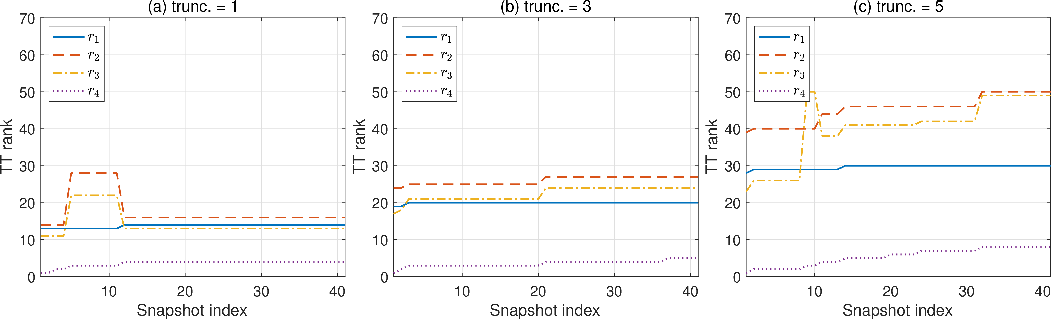
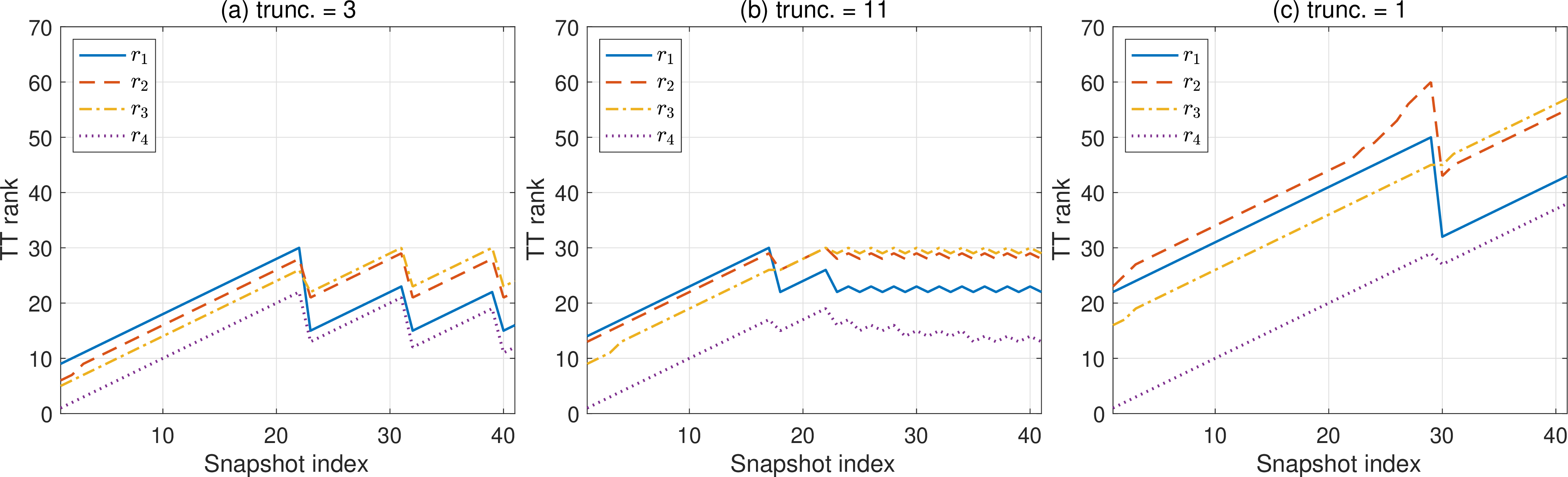
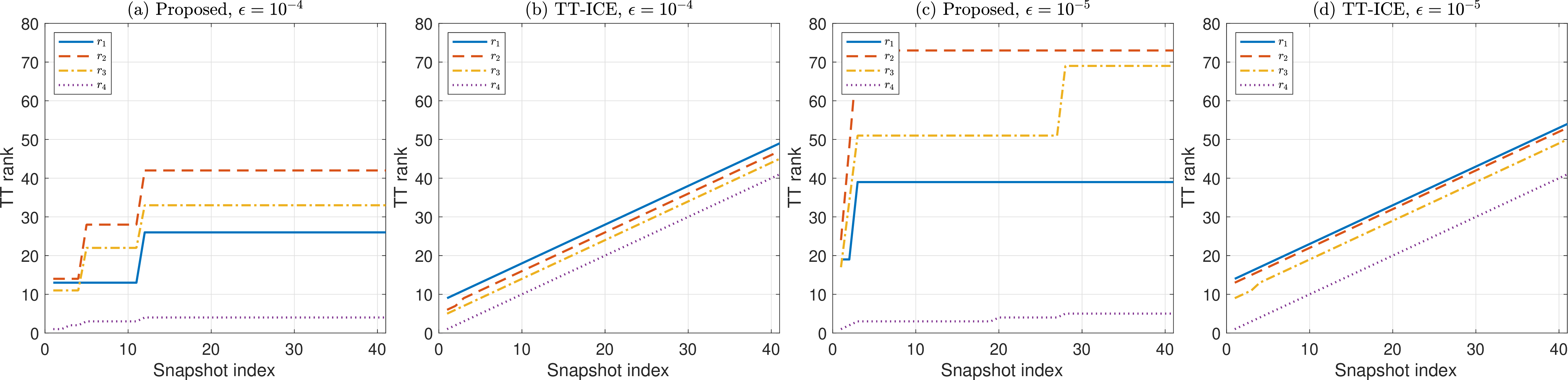
In Figures 3–4, we plot the evolution of the internal TT ranks of the accumulated tensor \({\boldsymbol{\psi}}\), together with the cumulative number of intermediate truncations performed during the iterative update process for the proposed method and TT-ICE. Across all three TT datasets, the TT ranks generated by the proposed method grow more slowly than those produced by TT-ICE. This indicates that the proposed enrichment strategy is more effective at controlling rank growth while maintaining comparable reconstruction accuracy. Moreover, the relatively small number of truncation events suggests that the observed rank control is achieved primarily through the enrichment procedure itself rather than through frequent rank-reduction operations.
To assess the role of intermediate truncation, Figure 5 repeats the first two homogeneous test cases without truncation. Compared with the corresponding results in Table 2, the accumulated TT ranks grow monotonically and become substantially larger. For example, at \(\epsilon=10^{-5}\), the ranks of the proposed method increase from \((20,27,24,5)\) with monitored truncation to \((39,73,69,5)\) without truncation, while the TT-ICE ranks increase from \((22,28,29,13)\) to \((54,53,50,41)\). Despite this substantial rank growth, the reconstruction errors remain comparable to those obtained with monitored truncation. These results confirm that intermediate truncation is beneficial for compression efficiency for both methods: it eliminates redundancy accumulated during the iterative enrichment process while maintaining the prescribed reconstruction accuracy.
| \(\epsilon\) | \(\epsilon_{\rm tt}\) | \(r_{\max}\) | Proposed time (s) | Proposed mean err. | TT-ICE time (s) | TT-ICE mean err. | Speedup | TT ranks \((r_1,\ldots,r_4)\) for \(\bpsi\), proposed/TT-ICE |
|---|---|---|---|---|---|---|---|---|
| \(10^{-4}\) | \(10^{-5}\) | \(30\) | \(1.353\times 10^{-1}\) | \(3.742\times 10^{-5}\) | \(2.294\times 10^{1}\) | \(3.612\times 10^{-5}\) | \(1.70\times 10^{2}\) | \((14,16,13,4)\) / \((16,22,24,12)\) |
| \(10^{-5}\) | \(10^{-6}\) | \(30\) | \(2.500\times 10^{-1}\) | \(6.683\times 10^{-6}\) | \(2.444\times 10^{1}\) | \(7.090\times 10^{-6}\) | \(9.78\times 10^{1}\) | \((20,27,24,5)\) / \((22,28,29,13)\) |
| \(10^{-6}\) | \(10^{-7}\) | \(60\) | \(2.356\times 10^{0}\) | \(7.507\times 10^{-7}\) | \(2.793\times 10^{1}\) | \(1.953\times 10^{-6}\) | \(1.19\times 10^{1}\) | \((30,50,49,8)\) / \((43,55,57,38)\) |
6.2.2 Changing-scattering medium↩︎
We consider the changing-scattering dataset with the configuration given in Table 1. As in the homogeneous example, the low-rank solver [24] generates the solution snapshots in low-rank matrix-factorized form. We then construct four TT versions of this dataset by converting each snapshot to TT format using four conversion tolerances \(10^{-2}\), \(10^{-3}\), \(10^{-4}\), and \(10^{-5}\), respectively. After conversion, each TT snapshot has mode size \(n=(100,100,16,32)\) and TT rank structure \((1,r_1,r_2,r_3,1)\). Compared with the homogeneous example, this dataset exhibits substantially larger TT ranks. The corresponding mean internal TT ranks \((r_1,r_2,r_3)\) of the four TT datasets are \[\begin{align} &(6.00,\,25.39,\,14.57), \qquad (10.00,\,51.24,\,22.24),\\ &(15.00,\,86.35,\,28.51), \qquad (21.00,\,116.94,\,32.00). \end{align}\]
Table 3 summarizes the reconstruction error, TT ranks of the accumulated tensor, and wall time for the four TT datasets. For each dataset, the same algorithmic tolerance \(\epsilon\), TT-rounding tolerance \(\epsilon_{\rm tt}\), and maximum TT rank \(r_{\max}\) are used by both methods, and the final postprocessing TT-rounding step is disabled. As in the homogeneous example, the two methods achieve comparable reconstruction errors across all four datasets, while the proposed method is consistently faster. For the dataset corresponding to \(\epsilon=10^{-3}\), \(\epsilon_{\rm tt}=10^{-4}\), and \(r_{\max}=60\), the proposed method attains a mean reconstruction error of \(8.03\times10^{-4}\), compared with \(7.29\times10^{-4}\) for TT-ICE, while reducing the wall time by a factor of 144. For the most stringent conversion tolerance \(10^{-5}\), with \(\epsilon=10^{-5}\), \(\epsilon_{\rm tt}=10^{-6}\), and \(r_{\max}=180\), both methods require substantially larger TT ranks. Nevertheless, the proposed method achieves a wall time of 3.92 seconds, compared with 22.94 seconds for TT-ICE, while also attaining a smaller mean reconstruction error.
The rank behavior is also consistent with that observed in the homogeneous example. TT-ICE generally produces larger TT ranks for the accumulated tensor \({\boldsymbol{\psi}}\), particularly at the interface between the physical modes and the sample mode. For the most stringent tolerance setting, the interface rank is 39 for TT-ICE and 13 for the proposed method. As in the homogeneous case, the observed speedup decreases as the tolerances are tightened, since the TT ranks of \({\boldsymbol{\psi}}\) increase and thereby raise the cost of the projection in the proposed method. Nevertheless, even for the most stringent tolerance setting, the proposed method remains more than five times faster than TT-ICE.
Figures 6–7 show the evolution of the internal TT ranks for both methods. Similar to the homogeneous example, the proposed method exhibits slower rank growth than TT-ICE across all four datasets, indicating that the incremental enrichment strategy is more effective at controlling redundant rank growth while maintaining comparable reconstruction accuracy.
| \(\varepsilon_{\rm alg}\) | \(\varepsilon_{\rm tt}\) | \(r_{\max}\) | Proposed time (s) | Proposed mean err. | TT-ICE time (s) | TT-ICE mean err. | Speedup | TT ranks \((r_1,\ldots,r_4)\) for \(\bpsi\), proposed/TT-ICE |
|---|---|---|---|---|---|---|---|---|
| \(10^{-2}\) | \(10^{-3}\) | \(60\) | \(9.910\times 10^{-2}\) | \(5.594\times 10^{-3}\) | \(2.558\times 10^{1}\) | \(2.158\times 10^{-3}\) | \(2.58\times 10^{2}\) | \((6,26,29,3)\) / \((54,60,57,51)\) |
| \(10^{-3}\) | \(10^{-4}\) | \(60\) | \(2.220\times 10^{-1}\) | \(8.055\times 10^{-4}\) | \(2.334\times 10^{1}\) | \(7.270\times 10^{-4}\) | \(1.05\times 10^{2}\) | \((10,51,41,4)\) / \((17,57,60,34)\) |
| \(10^{-4}\) | \(10^{-5}\) | \(100\) | \(3.172\times 10^{0}\) | \(8.650\times 10^{-5}\) | \(2.592\times 10^{1}\) | \(1.215\times 10^{-4}\) | \(8.17\times 10^{0}\) | \((17,100,80,6)\) / \((25,100,92,48)\) |
| \(10^{-5}\) | \(10^{-6}\) | \(180\) | \(9.509\times 10^{0}\) | \(9.481\times 10^{-6}\) | \(3.215\times 10^{1}\) | \(1.532\times 10^{-5}\) | \(3.38\times 10^{0}\) | \((24,174,176,13)\) / \((25,166,185,39)\) |


6.3 Applications in the ROM↩︎
We next apply the proposed incremental TT compression to build reduced bases for ROMs, following Section 5, on the three RTE benchmarks in Section 6.1. For each example, the low-rank solver in [24] generates the angular-flux snapshots in the form of low-rank matrix factorization: \[F_j=U_j\operatorname{diag}(s_j)V_j^T\in\mathbb{R}^{(4N_xN_y)\times (N_\theta N_{v_z})},\; U_j\in\mathbb{R}^{4N_xN_y\times r_j},\;V_j\in\mathbb{R}^{N_\theta N_{v_z}\times r_j},\] where \(U_j\) and \(V_j\) are low-rank factors collecting spatial and angular DOFs, respectively. In the projection-based ROM, these low-rank matrix factors are used directly as streaming input. In interpolation-based ROM, the same snapshots are converted to order-four TT tensors without additional truncation to demonstrate the flexibility of the proposed construction. In both cases, the online tests use five randomly sampled parameters outside the training set.
6.3.1 Applications in the projection-based ROM↩︎
We begin with the projection-based intrusive setting, where the reduced basis is used to project the affine operators, as well as the source term.
Incremental ROM construction from low-rank data. We construct the reduced basis directly from the streaming low-rank snapshots with residual enrichment threshold \(\epsilon=10^{-5}\), without prescribing a maximum TT rank. This setting highlights two advantages.
Low-rank data generation. Table 4 shows that the low-rank solver is faster in all three examples, with speedups ranging from \(1.48\) for the lattice case to \(4.70\) for the homogeneous case, and reduces the storage by factors between \(2.01\) and \(7.41\). The compressed low-rank solutions remain close to the full-rank references: the mean relative errors are between \(10^{-8}\) and \(10^{-6}\) for the angular flux \(f\), and between \(10^{-8}\) and \(10^{-7}\) for the scalar flux \(\rho\).
Incremental TT compression of the training data. Table 5 reports final accumulated TT ranks \((1,122,3,1)\), \((1,372,14,1)\), and \((1,1130,21,1)\) for the homogeneous, changing-scattering, and lattice examples, leading to ROM dimensions \(3\), \(14\), and \(21\), respectively. Relative to the full-rank training snapshot collection, the accumulated TT tensor further reduces the storage by factors of \(157.31\), \(40.88\), and \(21.72\), respectively.
After constructing the TT reduced basis \(U_{\rm rb}\), the affine linear operators and the source term are projected using the left-to-right TT contraction in Section 6.3.1.
| Example | Full solve time (s) | Low-rank solve time (s) | Speedup | Mean rank | Storage reduction | Low-rank \(f\) error | Low-rank \(\rho\) error |
|---|---|---|---|---|---|---|---|
| Homogeneous | \(2.348\times 10^{2}\) | \(4.996\times 10^{1}\) | \(4.70\) | \(67.0\) | \(7.41\) | \(6.887\times 10^{-8}\) | \(6.744\times 10^{-8}\) |
| Changing scattering | \(1.313\times 10^{2}\) | \(4.144\times 10^{1}\) | \(3.17\) | \(120.4\) | \(4.04\) | \(4.136\times 10^{-6}\) | \(2.992\times 10^{-7}\) |
| Lattice | \(3.015\times 10^{2}\) | \(2.034\times 10^{2}\) | \(1.48\) | \(140.2\) | \(2.01\) | \(2.256\times 10^{-6}\) | \(3.581\times 10^{-7}\) |
| Example | Training snapshots | Matrix size | Mean input rank | TT ranks of \(U_{\rm rb}\) | ROM dimension | ROM compression vs full data |
|---|---|---|---|---|---|---|
| Homogeneous | \(41\) | \(16384\times 512\) | \(65.37\) | \((1,122,3)\) | \(3\) | \(157.31\) |
| Changing scattering | \(51\) | \(10000\times 512\) | \(121.53\) | \((1,372,14)\) | \(14\) | \(40.88\) |
| Lattice | \(121\) | \(14400\times 288\) | \(140.76\) | \((1,1130,21)\) | \(21\) | \(21.72\) |
Online efficiency and accuracy: Table 6 summarizes the online performance of the projection-based ROM. The online stage consists of solving the reduced system and reconstructing the solution from the reduced coefficients. After model reduction, the reconstruction step becomes the dominant online cost. Nevertheless, the overall online speedups are substantial: \(5.30\times10^4\), \(6.76\times10^3\), and \(1.18\times10^4\) over the full-rank solver, and \(1.12\times10^4\), \(2.13\times10^3\), and \(8.08\times10^3\) over the low-rank solver for the homogeneous, changing-scattering, and lattice examples, respectively. This substantial acceleration is achieved without loss of accuracy: the mean relative errors are between \(10^{-6}\) and \(10^{-5}\) for both \(f\) and \(\rho\).
| Example | ROM solve time (s) | Scalar-flux reconstruction (s) | Speedup over full-rank solver | Speedup over low-rank solver | Relative error (\(f\)) | Relative error (\(\rho\)) |
|---|---|---|---|---|---|---|
| Homogeneous | \(6.486\times 10^{-4}\) | \(3.836\times 10^{-3}\) | \(5.300\times 10^{4}\) | \(1.119\times 10^{4}\) | \(1.612\times 10^{-5}\) | \(1.612\times 10^{-5}\) |
| Changing scattering | \(8.797\times 10^{-3}\) | \(1.692\times 10^{-2}\) | \(6.762\times 10^{3}\) | \(2.135\times 10^{3}\) | \(4.886\times 10^{-6}\) | \(2.910\times 10^{-6}\) |
| Lattice | \(2.084\times 10^{-4}\) | \(2.535\times 10^{-2}\) | \(1.181\times 10^{4}\) | \(8.075\times 10^{3}\) | \(2.702\times 10^{-6}\) | \(1.495\times 10^{-6}\) |
6.4 Applications in the interpolation-based ROM↩︎
To demonstrate the flexibility of our method, we consider the non-intrusive interpolation-based ROM using TT snapshots with nodal modes \((2N_x,2N_y,N_{v_z},N_\theta)\). The accumulated sample-augmented TT tensor provides both the reduced basis and the training coefficient core, which is interpolated online for new parameters.
Offline TT basis construction. Table 7 summarizes the offline construction. The final TT basis dimensions are \(3\), \(13\), and \(20\) for the homogeneous, changing-scattering, and lattice examples, respectively. The accumulated sample-augmented TT tensor remains highly compressed relative to the full-rank training snapshot collection, with storage reduction factors \(274.80\), \(69.54\), and \(22.79\). These factors are slightly larger than those obtained in the matrix-based projection-ROM construction for the first two examples and comparable for the lattice example.
| Example | Training snapshots | TT mode size | Mean TT input ranks | TT ranks of \(U_{\rm rb}\) | ROM dimension | ROM compression vs full data |
|---|---|---|---|---|---|---|
| Homogeneous | \(41\) | \(128\times128\times16\times32\) | \((1,67.71,65.37,32,1)\) | \((1,67,122,96,3)\) | \(3\) | \(274.80\) |
| Changing scattering | \(51\) | \(100\times100\times16\times32\) | \((1,52.41,121.53,32,1)\) | \((1,55,359,288,13)\) | \(13\) | \(69.54\) |
| Lattice | \(121\) | \(120\times120\times12\times24\) | \((1,120,140.76,24,1)\) | \((1,120,1130,408,20)\) | \(20\) | \(22.79\) |
Online coefficient interpolation and output reconstruction. We use the same randomly sampled test parameters as in Section 6.3.1. Following Section 5.3, the coefficient core is interpolated using cubic splines for the one-parameter homogeneous and changing-scattering examples, and tensor-product cubic splines in \((\sigma_s,\sigma_a)\) for the lattice example. The angular flux and scalar flux are then recovered from the compressed TT representation by contractions with the TT basis and the angular quadrature weights, respectively.
Table 8 reports the average online cost and accuracy over the five test parameters. The interpolation cost is negligible, while solution reconstruction from the reduced coefficients dominates the online cost. Overall, the interpolation-based ROM achieves speedups of \(3.12\times 10^{4}\), \(8.50\times 10^{3}\), and \(2.85\times 10^{3}\) over the full-rank solver, and \(6.65\times 10^{3}\), \(2.68\times 10^{3}\), and \(1.92\times 10^{3}\) over the low-rank solver for the homogeneous, changing-scattering, and lattice examples, respectively. The mean relative errors are between \(10^{-6}\) and \(10^{-5}\) for both \(f\) and \(\rho\).
| Example | Coefficient interpolation (s) | Scalar-flux evaluation (s) | Speedup over full-rank solver | Speedup over low-rank solver | Relative error (\(f\)) | Relative error (\(\rho\)) |
|---|---|---|---|---|---|---|
| Homogeneous | \(3.050\times 10^{-4}\) | \(7.212\times 10^{-3}\) | \(3.123\times 10^{4}\) | \(6.646\times 10^{3}\) | \(5.109\times 10^{-6}\) | \(3.985\times 10^{-6}\) |
| Changing scattering | \(1.797\times 10^{-4}\) | \(1.527\times 10^{-2}\) | \(8.497\times 10^{3}\) | \(2.682\times 10^{3}\) | \(8.072\times 10^{-6}\) | \(4.652\times 10^{-6}\) |
| Lattice | \(1.131\times 10^{-2}\) | \(9.451\times 10^{-2}\) | \(2.849\times 10^{3}\) | \(1.922\times 10^{3}\) | \(1.080\times 10^{-5}\) | \(2.982\times 10^{-6}\) |
7 Conclusions↩︎
We developed a deterministic incremental TT compression algorithm for streaming high-dimensional data that are already available in TT or low-rank matrix factorization formats. For streaming TT data, the method updates an accumulated TT representation directly at the core level through projection, residual orthogonalization, and adaptive enrichment. In this way, it avoids reconstructing both the incoming tensors and the accumulated full tensor, preserving the computational advantage of low-rank representations. We also established approximation error bounds and computational complexity estimates for the proposed approach, and demonstrated how the accumulated TT representation can be exploited to construct ROMs directly from low-rank data through operations on TT cores.
Numerical experiments on parametric radiative transfer equations confirmed the accuracy and efficiency of the proposed method. The proposed incremental compression algorithm achieved reconstruction accuracy comparable to TT-ICE while substantially reducing wall time. In addition, the low-rank ROMs built from the accumulated TT produced accurate reduced solutions with significant online speedups and storage reductions.
Several directions are worth further exploration. These include extending the projection-based ROM construction to non-affine or nonlinear operators through tensor hyper-reduction. Another promising direction is to develop more efficient dataset-level parallel TT compression algorithms by combining the proposed incremental TT compression with ideas from TT-ICE.
Acknowledgments↩︎
Part of this research was performed while W. Guo was visiting the Institute for Pure and Applied Mathematics (IPAM), which is supported by the National Science Foundation (Grant No. DMS-1925919/2422832). Z. Peng was partially supported by the Hong Kong Research Grants Council grants Early Career Scheme 26302724 and General Research Fund 16306825.
Declaration of generative AI and AI-assisted technologies in the writing process↩︎
During the preparation of this work, the authors used AI-assisted tools to assist with code development, debugging, grammar checking, and readability improvement. All numerical experiments, mathematical formulations, algorithms, proofs, results, and conclusions were reviewed and verified by the authors. The authors assume responsibility for all content.
8 Proof of Lemma 4↩︎
Consider two \(d\)-dimensional tensors \(\boldsymbol{X},\,\boldsymbol{Y}\in\mathbb{R}^{n_1\times n_2\times\cdots\times n_d}\) represented in TT format given by \[\boldsymbol{X} = {\mathcal{U}}_1\cdots{\mathcal{U}}_{i-1}{\mathcal{W}}_{i}^X\cdots{\mathcal{W}}_{d}^X,\quad \boldsymbol{Y} = {\mathcal{U}}_1\cdots{\mathcal{U}}_{i-1}{\mathcal{W}}_{i}^Y\cdots{\mathcal{W}}_{d}^Y\] with TT-ranks \(\{r_0,r_1,\ldots,r_{i-1},r_i^X,\ldots, r_{d}^X\}\) and \(\{r_0,r_1,\ldots,r_{i-1},r_i^Y,\ldots, r_{d}^Y\}\), respectively. Assume that the shared first \(i-1\) cores \({\mathcal{U}}_1,\dots,{\mathcal{U}}_{i-1}\) are left-orthogonal. Let \(W_i^X\) and \(W_i^Y\) denote the left unfoldings of the \(i\)-th cores \({\mathcal{W}}_{i}^X\) and \({\mathcal{W}}_{i}^Y\), respectively. If \(W_i^X\) and \(W_i^Y\) are orthogonal in the sense that \[(W_i^X)^T W_i^Y = \mathbf{0},\] then we show that the Frobenius inner product of the tensors is zero: \[\langle \boldsymbol{X}, \boldsymbol{Y} \rangle_F = 0.\]
Let the interface matrix \[U_{\le i-1}\in \mathbb{R}^{(n_1\cdots n_{i-1})\times r_{i-1}}\] denote the contraction of the shared first \(i-1\) cores, and let the interface matrices \[W_{\ge i+1}^X \in \mathbb{R}^{(n_{i+1}\cdots n_d)\times r_i^X}, \qquad W_{\ge i+1}^Y \in \mathbb{R}^{(n_{i+1}\cdots n_d)\times r_i^Y}\] denote the contractions of the remaining cores \(i+1,\dots,d\) for \(\boldsymbol{X}\) and \(\boldsymbol{Y}\), respectively. Then, the mode-\(i\) unfolding of \(\boldsymbol{X}\) and \(\boldsymbol{Y}\) can be written as \[X_{\langle i\rangle} = (U_{\le i-1}\otimes I_{n_i})\,W_i^X\,(W_{\ge i+1}^X)^T,\] \[Y_{\langle i\rangle} = (U_{\le i-1}\otimes I_{n_i})\,W_i^Y\,(W_{\ge i+1}^Y)^T,\] where \(\otimes\) denotes the Kronecker product and \(I_s\) denotes the \(s\)-by-\(s\) identity matrix; see [26].
Therefore, \[\begin{align} \langle \boldsymbol{X},\boldsymbol{Y}\rangle_F &= \left\langle X_{\langle i\rangle},Y_{\langle i\rangle}\right\rangle_F \\ &= \operatorname{tr}\!\left( \bigl((U_{\le i-1}\otimes I_{n_i})W_i^X (W_{\ge i+1}^X)^T\bigr)^T \bigl((U_{\le i-1}\otimes I_{n_i})W_i^Y (W_{\ge i+1}^Y)^T\bigr) \right) \\ &= \operatorname{tr}\!\left( W_{\ge i+1}^X (W_i^X)^T (U_{\le i-1}\otimes I_{n_i})^T (U_{\le i-1}\otimes I_{n_i}) W_i^Y (W_{\ge i+1}^Y)^T \right). \end{align}\] Since the first \(i-1\) shared cores are left-orthogonal, \(U_{\le i-1}^T U_{\le i-1}=I_{r_{i-1}},\) \[(U_{\le i-1}\otimes I_{n_i})^T (U_{\le i-1}\otimes I_{n_i}) = (U_{\le i-1}^T U_{\le i-1})\otimes I_{n_i} = I_{r_{i-1}n_i}.\] Thus, \[\langle \boldsymbol{X},\boldsymbol{Y}\rangle_F = \operatorname{tr}\!\left( W_{\ge i+1}^X (W_i^X)^T W_i^Y (W_{\ge i+1}^Y)^T \right).\] Finally, given the orthogonality condition \((W_i^X)^T W_i^Y = 0\), it immediately follows that \[\langle \boldsymbol{X},\boldsymbol{Y}\rangle_F=0.\]