1 Introduction↩︎

Prophet inequalities are a fundamental model of online decision-making and optimal stopping [1]. A decision-maker sequentially observes rewards and must irrevocably decide when to stop and accept the current reward. The benchmark is the prophet, who observes all realizations in advance and obtains the maximum reward. The goal is to design a stopping rule whose expected reward is competitive with this prophet benchmark. This framework has attracted significant attention due to its rich mathematical structure and its broad range of applications, including posted-price mechanisms [2], online ad allocation [3], and hiring processes in labor markets [4].

Classical prophet inequalities assume that the reward distributions are known. Under this assumption, for i.i.d.reward distributions, [5] established the classical \(1-1/e\) guarantee, and subsequent work characterized the optimal full-information i.i.d.worst-case constant \(\kappa\approx0.745\) [6], [7].

However, full distributional knowledge is rarely available in applications. This has motivated a growing literature on prophet inequalities with unknown distributions. A central message of this literature is that, for arbitrary unknown distributions, learning is severely limited without sufficient offline samples: in the i.i.d.setting, one cannot improve over the competitive ratio \(1/e\) with \(o(n)\) offline samples [8]. Achieving near-optimal worst-case guarantees for arbitrary distributions requires substantial distributional information, such as \(\Theta(n)\) or more offline samples [9]. Thus, in the absence of structure, learning prophet inequalities is constrained by strong sample-complexity barriers.

A complementary perspective is to seek distribution-specific asymptotic performance beyond distribution-free worst-case guarantees. [10] pursue this direction using nonparametric relative-rank-based rules, establishing first-order asymptotic optimality in the Gumbel and reverse-Weibull domains. However, because their rules use only relative ranks, they cannot exploit parametric information in the observed reward values. This restriction is especially pronounced in the Fréchet heavy-tailed regime: no relative rank-based rule can attain the full-information Fréchet heavy-tailed limit, as discussed later. Even where the relative rank-based framework applies, its nonparametric rates can be slower than those achievable under stronger parametric structure.

Another closely related direction is online learning in structured prophet inequality models. [11] study prophet inequalities under a linear reward structure with an unknown parameter and a known feature distribution. Their objective, however, is to recover the classical distribution-agnostic guarantee of \(1-1/e\). This guarantee is robust but not distribution-specific: it can be strictly below the optimal ratio achievable within a given distribution class, and is also below the optimal full-information i.i.d. worst-case constant \(\kappa\approx0.745\).

These works motivate the following question: Can one exploit parametric distributional structure to learn the unknown parameter online and match the full-information distribution-specific benchmark? We answer this question affirmatively for an exponential-type parametric family, which includes light-tailed, heavy-tailed, and bounded-support models such as exponential, Pareto, and bounded-support power-family distributions. Our goal is not to recover a distribution-agnostic worst-case constant, but to learn the parameter from online observations alone and match the full-information distribution-specific asymptotic competitive ratio. Our main contributions are summarized as follows.

• Optimal full-information asymptotics. We characterize the asymptotically optimal competitive ratio for the proposed exponential-type family when the distribution parameter \(\theta\) is known. In the unbounded-support case, the limiting optimal ratio is \(\frac{1}{\Gamma(1-c_+/\theta)} \left(\frac{\theta}{\theta-c_+}\right)^{c_+/\theta},\) which is governed by the endpoint-growth parameter \(c_+\). In the bounded-support case, the optimal competitive ratio converges to \(1\).

• Online learning with asymptotically optimal guarantees. We propose a confidence-based dynamic-programming policy for online learning. The policy first estimates the unknown distribution parameter from an initial exploration phase, constructs an upper confidence bound, and then applies the corresponding plug-in DP thresholds. By exploiting the explicit parametric structure, the proposed policy achieves the same asymptotically optimal competitive ratio as the optimal known-parameter policy, using only online observations and no external offline samples.

• Distribution-specific convergence guarantees. We derive refined convergence guarantees for representative distributions, including exponential, Pareto, and bounded-support power-family rewards. For exponential and bounded-support examples, our policy matches the convergence rates of the corresponding full-information optimal policies. For Pareto heavy-tailed rewards, we obtain a Pareto-specific convergence guarantee showing convergence to the full-information limiting ratio. These results show how tail or endpoint structure governs the speed of convergence, and are supported by numerical experiments.

2 Related Work↩︎

2.0.0.1 Prophet inequalities with known distributions.

The classical prophet inequality was initiated by [12]. Building on this line of work, [13] showed that a single threshold achieves the optimal \(1/2\) competitive ratio for independent non-identical rewards. For i.i.d. rewards, [5] established stronger guarantees of \(1-1/e\), and later work characterized the optimal full-information i.i.d. competitive ratio as constant \(\kappa\approx 0.745\) [6]. These works assume that the reward distribution is known, whereas our focus is on learning the unknown parameter of a structured distribution online.

2.0.0.2 Unknown distributions and sample-based prophet inequalities.

[8] studied i.i.d. prophet inequalities with an unknown distribution and showed that, with no samples or even \(o(n)\) samples, the best possible ratio is \(1/e\). They also showed that \(n-1\) samples yield a \(1-1/e\) guarantee and that \(O(n^2)\) samples suffice to approach the optimal full-information constant \(\kappa\). [9] improved the i.i.d. sample complexity to \(O(n/\varepsilon^6)\) for an \(\kappa-O(\varepsilon)\) guarantee. Our work is complementary: instead of using external offline samples from an arbitrary distribution, we exploit a parametric form and learn the unknown parameter from the online observations.

2.0.0.3 Rank-based stopping and extreme-value theory.

[10] studied optimal stopping for i.i.d. observations from an unknown continuous distribution using relative-rank-based rules. Their analysis is closely connected to extreme-value theory: they establish first-order asymptotic optimality in the Gumbel and reverse-Weibull domains, whereas in the Fréchet domain vanishing relative regret is impossible. Our endpoint regularity conditions admit a similar extreme-value interpretation. In contrast to their nonparametric, rank-based approach, we exploit parametric rewards to attain optimal distribution-specific asymptotic ratios across light-tailed, heavy-tailed, and bounded-support models within our family, with sharper convergence rates in canonical examples.

2.0.0.4 Structured and parametric learning in prophet inequalities.

[11] study prophet inequalities under a linear reward structure with an unknown parameter and a known feature distribution, and recover the classical \(1-1/e\) guarantee. Their setting is structurally different from ours, and the resulting guarantee is distribution-agnostic rather than distribution-specific. In particular, it can be below the optimal ratio for a given distribution class and the optimal worst-case full-information i.i.d. constant \(\kappa\approx0.745\). Parametric learning in optimal stopping was also studied by [14] for exponential rewards with an unknown mean. In contrast, we consider finite-horizon prophet inequalities for a parametric exponential-type family with an unknown distribution parameter, and learn this parameter online to achieve the optimal distribution-specific competitive ratio.

3 Problem Statement↩︎

We consider the classical prophet-inequality framework over a finite horizon \(n\in\mathbb{N}\), where an i.i.d. nonnegative random reward \(X_i\ge 0\) is revealed sequentially to the decision maker (or gambler) at each stage \(i\in[n]\). For the reward distribution, we consider a exponential-type parametric family, defined as follows.

3.0.0.1 Online stopping objective.

Let \(X_1,\dots,X_n\) be i.i.d. rewards drawn from \(F_\theta\) under an unknown parameter \(\theta\). A policy is a stopping time \(\tau\in\{1,\dots,n\}\cup\{n+1\}\) adapted to the sequential observations \((X_t)_{t\ge 1}\): after observing \(X_t\), the decision-maker either stops and receives reward \(X_t\), or continues to \(t+1\) (and can never return to \(t\)). We define \(X_{n+1}:=0\) to be the reward for the case when the stopping rule continues over all periods in \([n]\). The benchmark is the prophet value \(\mathrm{OPT}(\theta):=\mathbb{E}_\theta[\max_{t\in[n]} X_t]\), and the goal is to design a policy (not knowing \(\theta\)) with a large competitive ratio \[\mathrm{CR}_n(\tau;\theta)= \frac{\mathbb{E}_\theta[X_\tau]}{\mathrm{OPT}(\theta)},\] where \(\mathbb{E}_\theta\) denotes expectation under \(X_1,\dots,X_n \stackrel{\mathrm{i.i.d.}}{\sim} F_\theta\); we write \(\mathbb{E}\) when \(\theta\) is clear.

4 Preliminary Results↩︎

In this section, we derive an estimation guarantee for the exponential-type parametric family and introduce benchmark policies for comparison.

4.1 Estimator and Confidence Bound↩︎

Let \(Y_i := \phi(X_i)\) for \(i \in [n]\). Then \(Y_i \sim \mathrm{Exp}(\theta)\), where \(\mathrm{Exp}(\theta)\) denotes the exponential distribution with rate \(\theta\). Since an exponential random variable with rate \(\theta\) has mean \(1/\theta\), we have \(\theta=\frac{1}{\mathbb{E}[Y_i]}.\) This motivates the plug-in estimator \(\widehat{\theta}_m =\left(\frac{1}{m}\sum_{i=1}^m Y_i\right)^{-1},\) and the corresponding estimated cumulative distribution function \(F_{\widehat{\theta}_m}(x)=1-\exp\bigl(-\widehat{\theta}_m\phi(x)\bigr).\) We next provide a confidence bound for \(\widehat{\theta}_m\); see Appendix 10.1 for the proof.

4.2 Baseline Policies↩︎

We next discuss two natural baseline policies. The first is a distribution-specific nonparametric baseline based on relative ranks. The second is a distribution-agnostic sample-based baseline using the confidence bound from the previous section.

4.2.0.1 Rank-based distribution-specific baseline.

A natural nonparametric baseline is the relative-rank-based rule of [10], which uses only the relative ranks of the observations. It achieves first-order asymptotic optimality, in the sense of vanishing relative regret, in the Gumbel and reverse-Weibull domains. Specifically, for the exponential distribution, their guarantees imply \(\mathrm{CR}_n(\tau;\theta) \ge 1-O\!\left({\log\log\log n}/{\log n}\right),\) whereas for the uniform distribution on a bounded interval, they imply \(\mathrm{CR}_n(\tau;\theta) \ge 1-O\!\left({\log n}/{n}\right),\) as \(n\to\infty\). These convergence rates towards the optimal limit of \(1\) are useful nonparametric baselines, but they are not tailored to parametric subfamilies where sharper rates are possible. Moreover, as discussed later, the relative rank-based framework does not recover the full-information distribution-specific limit in the Fréchet heavy-tailed domain.

4.2.0.2 Distribution-agnostic sample-based baseline.

Another natural reference is the Samples-CFHOV rule of [9]. We adapt it to our online setting by estimating the unknown parameter from the initial observations and then applying sample-based thresholds under the estimated model. With a suitable exploration length, this baseline achieves a competitive ratio arbitrarily close to the optimal i.i.d.worst-case constant \(\kappa\approx0.745\); see Appendix 10.5. However, it remains distribution-agnostic and does not target the sharper full-information distribution-specific baseline.

Our main policy instead uses confidence-based DP thresholds for online learning, tailored to the exponential-type family. This allows us to exploit the parametric structure and achieve the optimal distribution-specific asymptotic competitive ratio, including for heavy-tailed Pareto-type rewards.

5 Optimal Competitive Ratio↩︎

To characterize the full-information asymptotic benchmark, we impose the following endpoint regularity condition.

5.0.0.1 Endpoint indices and finite prophet benchmarks.

Since \(\phi\) is strictly increasing, its inverse \(\psi\) is also strictly increasing. Hence \(\psi'(y)\ge 0\) wherever the derivative exists, and the endpoint indices \(c_+\) and \(c_-\) are necessarily nonnegative. The restriction \(c_+<\theta\) is imposed only in the unbounded-endpoint case. It is an integrability condition: if \(c_+>\theta\), then¹ \(\mathbb{E}[X_i]=\infty\), and in the boundary case \(c_+=\theta\), the mean may still be infinite in general; see Appendix 10.3. In contrast, when \(x_F<\infty\), the support is bounded above, so \(\mathbb{E}[X_i]\le x_F<\infty\). Therefore no analogous restriction on \(c_-\) is needed.

5.0.0.2 Canonical examples.

This family includes several common distributions as special cases. In the unbounded-endpoint case, the exponential distribution corresponds to \(\phi(x)=x\) on \([0,\infty)\), for which \(\psi(y)=y\) and hence \(c_+=0\). Another example is the Pareto family, obtained from \(\phi(x)=\log(x/x_{0})\) on \([x_{0},\infty)\). In this case \(\psi(y)=x_{0}e^y\), so \(c_+=1\). In the bounded-support case, a natural example is bounded-support power-family distributions with \(\phi(x)=\log\!\left(\frac{x_F-x_0}{x_F-x}\right)\) for \(x\in[x_0,x_F),\) for which \(\bar\psi(y)=(x_F-x_0)e^{-y}\) and hence \(c_-=1\). This includes the uniform distribution on \([x_0,x_F]\) as the special case \(\theta=1\).

Under Assumption 1, we now analyze the asymptotically optimal competitive ratio for the exponential-type family. The characterization depends on the tail parameter \(c_+\) in the unbounded-support case and on the endpoint parameter \(c_-\) in the bounded-support case. We first provide the optimal ratio for the unbounded support case, and the proof is provided in Appendix 10.6.

We next provide the optimal ratio for the bounded-support case; the proof is in Appendix 10.7.

6 Confidence-based Dynamic-Programming Policy for Online Learning↩︎

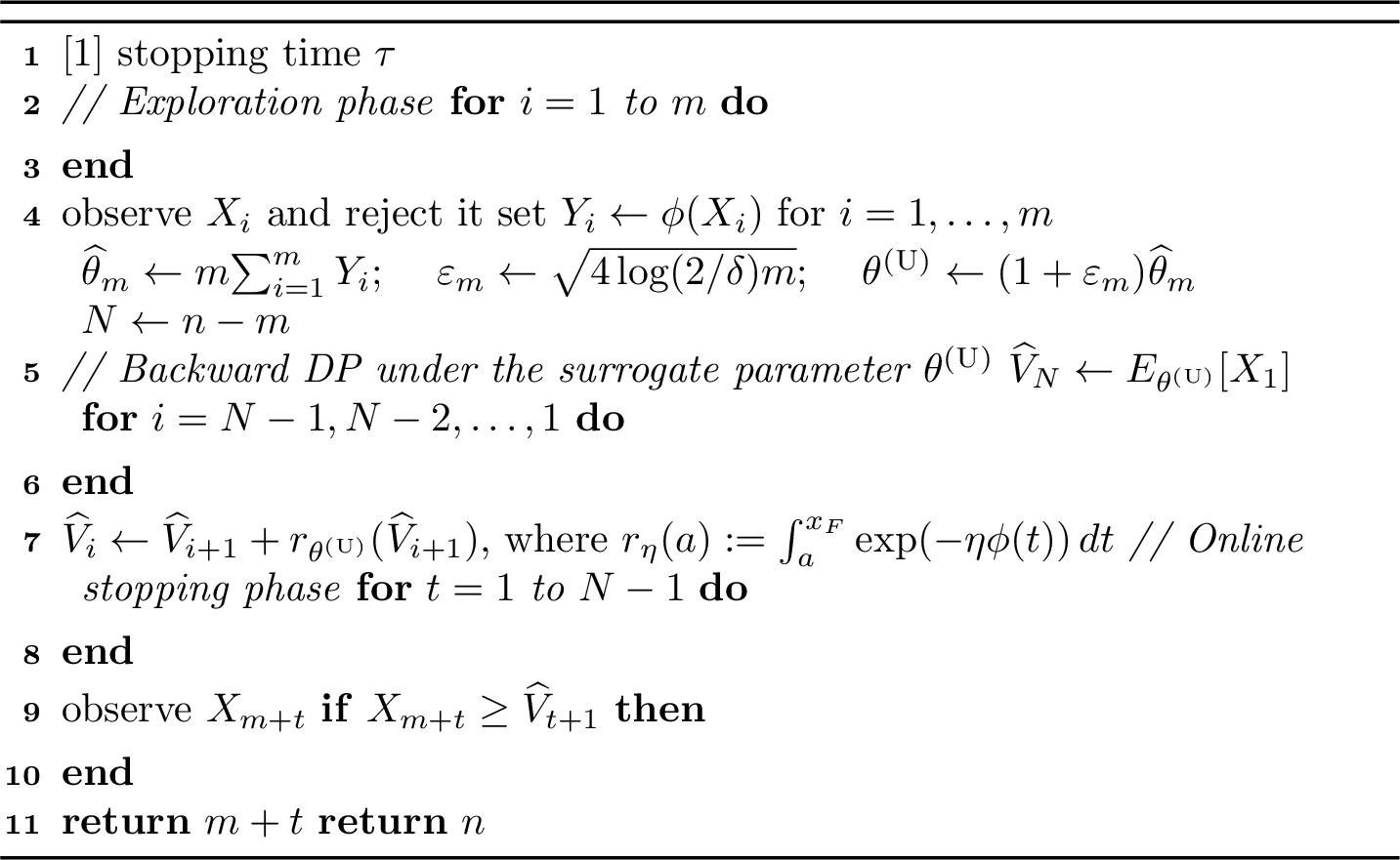
To target the distribution-specific optimal competitive ratio analyzed in the previous section, we propose a confidence-based dynamic-programming (DP) policy for online learning; see Algorithm 1. The algorithm first uses the initial \(m\) periods for exploration, during which it only collects observations. It then computes the estimator \(\widehat{\theta}_m\), constructs an upper confidence bound \(\theta^{(U)}\), and applies the DP policy obtained by plugging \(\theta^{(U)}\) into the value recursion.

Although \(\theta^{(U)}\) is an upper confidence bound, a larger rate parameter makes the reward distribution stochastically smaller. Thus, the surrogate model yields conservative continuation values and lower plug-in DP thresholds on the event \(\theta^{(U)}\ge\theta\). This prevents the policy from being overly selective under parameter uncertainty.

6.1 Unbounded-support case↩︎

We first analyze the guarantee of Algorithm 1 in the unbounded-support case, where \(x_F=\infty\), under Assumption 1(i). The proof of the following theorem is given in Appendix 10.8.

Theorem 6 shows that Algorithm 1 attains the full-information optimal ratio of Theorem 3 in the unbounded-support case, up to the confidence factor \(1-\delta\). Since \(\delta\in(0,1)\) is arbitrary, the limiting guarantee can be made arbitrarily close to \(\rho(c_+,\theta)\).

When \(c_+>0\), the extreme-value index is \(\gamma=c_+/\theta\in(0,1)\), placing the model in the Fréchet heavy-tailed domain, where the guarantees of relative rank-based rule in [10] do not apply. Moreover, Appendix 10.13 shows that any relative rank-based rule is asymptotically bounded away from the full-information Fréchet benchmark. Thus, exploiting parametric reward values is essential for recovering the optimal heavy-tailed limit.

6.2 Bounded-support case↩︎

Now we analyze the guarantee of Algorithm 1 in the bounded-support case, where \(x_F<\infty\), under Assumption 1(ii). The proof of the following theorem is given in Appendix 10.9.

In Theorem 7, we show that our algorithm achieves asymptotically optimal competitive ratio in the bounded-support case, matching the optimal ratio in Theorem 4.

7 Canonical Examples: Exponential, Pareto, and Bounded-Support Families↩︎

In this section, we instantiate the general framework for exponential, Pareto, and bounded-support models. In each case, the explicit form of \(\phi\) allows us to compute the tail integral \(r_\eta(a)\), derive the corresponding plug-in DP recursion, and obtain sharper model-specific convergence guarantees. We also compare these rates with those of [10].

7.1 Exponential Distribution↩︎

We first investigate the case of an exponential reward distribution such that \(X_i\sim \mathrm{Exp}(\theta)\) with \(\theta>0\). This corresponds to \(\phi(x)=x\) on \([0,\infty)\), so that \(F_\theta(x)=1-\exp(-\theta x)\) for \(x\ge 0.\) This distribution falls into the unbounded-endpoint case and satisfies \(c_+=0\). Hence, the limiting optimal competitive ratio is \(\rho(0,\theta)=1\).

For the estimated value update in Line [line:DP] of Algorithm 1, note that for any \(a\ge 0\), \(r_\eta(a) = \int_a^\infty e^{-\eta\phi(t)}\,dt = \int_a^\infty e^{-\eta t}\,dt = \frac{e^{-\eta a}}{\eta}.\) Hence the plug-in DP recursion becomes \[\begin{align} \label{eq:DP95exp} \widehat V_N = \mathbb{E}_{\theta^{(\mathrm U)}}[X_1] = \frac{1}{\theta^{(\mathrm U)}},\quad \widehat V_i = \widehat V_{i+1} + \frac{\exp\!\left(-\theta^{(\mathrm U)}\widehat V_{i+1}\right)}{\theta^{(\mathrm U)}}, \qquad i=1,\dots,N-1. \end{align}\tag{1}\]

That is, at each stage \(t\in [N]\), the algorithm uses the corresponding plug-in DP threshold determined by the above recursion. The following theorem gives its competitive ratio; the proof is in Appendix 10.10.

The three error terms have different origins. The first term comes from estimating the unknown parameter, the second from discarding the first \(m\) observations for exploration, and the last term is the intrinsic full-information finite-horizon gap. In particular, Theorem 8 implies that Algorithm 1 is asymptotically optimal in the exponential case, achieving the optimal competitive ratio \(1\) from Theorem 3 when \(c_+=0\). Optimizing the exploration length \(m\) then yields the following convergence rate.

By taking \(\delta=\delta_n=1/n\), the estimation and exploration errors become lower order, and the overall competitive-ratio gap is dominated by the intrinsic full-information finite-horizon gap of order \(1/\log n\). Thus, the rate matches that of the optimal stopping policy when the distribution parameter is known, as shown below. Compared with the relative rank-based method of [10], whose guarantee for the exponential case is \(O(\log\log\log n/\log n)\), our parametric approach exploits the exponential-type structure to attain the full-information-optimal \(O(1/\log n)\) rate, thereby removing the extra \(\log\log\log n\) factor. The precise full-information convergence rate is given in the following proposition, whose proof is provided in Appendix 10.11.

7.2 Pareto Distribution↩︎

We now consider Pareto rewards \(X_i\sim \mathrm{Pareto}(\theta)\) with shape parameter \(\theta>1\) (otherwise, \(\mathbb{E}[X_i]=\infty\)), and scale parameter \(x_0>0\). This corresponds to \(\phi(x)=\log(x/x_0)\) for \(x\ge x_0,\) so that \(F_\theta(x)=1-\left(\frac{x_0}{x}\right)^\theta\) for \(x\ge x_0.\) This distribution has an unbounded endpoint and satisfies \(c_+=1\).

For the estimated value update in Line [line:DP] of Algorithm 1, note that for any \(a\ge x_0\) and \(\eta>1\), this gives \(r_\eta(a) = x_0^\eta\int_a^\infty t^{-\eta}\,dt = \frac{x_0^\eta}{\eta-1}a^{1-\eta}.\) Hence, the plug-in DP recursion becomes \[\begin{align} \label{eq:DP95pareto} \widehat V_N = \mathbb{E}_{\theta^{(\mathrm U)}}[X_1] = \frac{\theta^{(\mathrm U)}x_0}{\theta^{(\mathrm U)}-1}, \quad \widehat V_i = \widehat V_{i+1} + \frac{x_0^{\theta^{(\mathrm U)}}}{\theta^{(\mathrm U)}-1} \widehat V_{i+1}^{\,1-\theta^{(\mathrm U)}}, \qquad i=1,\dots,N-1. \end{align}\tag{2}\] The following theorem presents the competitive ratio achieved by this algorithm; the proof is in Appendix 10.12.

In particular, Theorem 10 implies that Algorithm 1 is asymptotically optimal in the Pareto case, achieving the optimal competitive ratio of \(\rho(1,\theta)=\frac{\left(\frac{\theta}{\theta-1}\right)^{1/\theta}}{\Gamma(1-1/\theta)}\) in Theorem 3. Optimizing the exploration length \(m\) then yields the following convergence rate.

In contrast, the relative rank-based framework of [10] does not recover the full-information Pareto-specific limit in the Fréchet heavy-tailed regime: indeed, no relative rank-based rule can attain \(\rho(1,\theta)\) for Pareto rewards, as shown in Appendix 10.13. Our algorithm attains this optimal asymptotic competitive ratio, and this separation is also reflected in the experiments below.

Unlike the exponential case, the full-information Pareto DP ratio has no \(1/\log n\) bottleneck; it approaches \(\rho(1,\theta)\) with a smaller finite-horizon correction of order \(\log n/n\). Thus, the rate in Corollary 2 is governed by the learning and exploration errors. The corresponding full-information rate is provided in Appendix 10.14.

7.3 Bounded-Support Power Family↩︎

We next investigate the bounded-support power family \(\phi(x)=\log\!\left(\frac{x_F-x_0}{x_F-x}\right)\) for \(x\in[x_0,x_F),\) for which \(F_\theta(x) = 1-\left(\frac{x_F-x}{x_F-x_0}\right)^\theta\) for \(x\in[x_0,x_F]\) for \(\theta>0\). This includes the uniform distribution on \([x_0,x_F]\) as the special case \(\theta=1\).

For the estimated value update in Line [line:DP] of Algorithm 1, note that for any \(a\in[x_0,x_F]\), \(r_\eta(a) = \int_a^{x_F} e^{-\eta\phi(t)}\,dt = \int_a^{x_F}\left(\frac{x_F-t}{x_F-x_0}\right)^\eta dt = \frac{(x_F-a)^{\eta+1}}{(\eta+1)(x_F-x_0)^\eta}.\) Hence the plug-in DP recursion becomes \[\begin{align} \label{eq:DP95uniform95family} \widehat V_N &= \mathbb{E}_{\theta^{(\mathrm U)}}[X_1] = x_0+\frac{x_F-x_0}{\theta^{(\mathrm U)}+1} = x_F-\frac{\theta^{(\mathrm U)}}{\theta^{(\mathrm U)}+1}(x_F-x_0),\\ \widehat V_i &= \widehat V_{i+1} + \frac{(x_F-\widehat V_{i+1})^{\theta^{(\mathrm U)}+1}}{(\theta^{(\mathrm U)}+1)(x_F-x_0)^{\theta^{(\mathrm U)}}}, \qquad i=1,\dots,N-1. \end{align}\tag{3}\]

The following theorem presents the competitive ratio achieved by this algorithm; the proof is in Appendix 10.15.

In particular, for the uniform distribution, corresponding to the special case \(\theta=1\), Theorem 11 with \(\delta=1/n\) yields an \(O(1/n)\) convergence rate toward the optimal competitive ratio \(1\). This improves over the \(O(\log n/n)\) rate of the relative rank-based approach of [10].

More generally, the rate \(n^{-1/\theta}\) is already the intrinsic finite-horizon rate of the optimal full-information DP policy. The following proposition shows that even when the parameter \(\theta\) is known, the competitive ratio approaches its limiting value \(1\) at order \(n^{-1/\theta}\). Thus, up to the multiplicative factor \(1-\delta\), the rate in Theorem 11 matches the full-information finite-horizon rate.

8 Experiments↩︎

We evaluate Algorithm 1 on exponential, Pareto, and bounded-support rewards, and compare it with three baselines: the secretary-type Gusein-Zade rule [8], [17], the online Samples-CFHOV variant (Algorithm 3), and the relative rank-based GZ-RANK rule of [10]. Figure 2 shows that our algorithm consistently approaches the corresponding optimal asymptotic ratio and performs favorably against the baselines, especially in the Pareto case where rank-based methods do not guarantee asymptotic optimality. The Samples-CFHOV curve starts later because its required exploration length exceeds the horizon for small \(n\). The detailed setup is described in Appendix 10.17.

9 Conclusion↩︎

We studied prophet inequalities for an exponential-type parametric family with an unknown parameter. We characterized the full-information distribution-specific asymptotic benchmark and proposed a confidence-based DP learning policy that attains it using only online observations. Our example-specific analyses and experiments show how parametric structure enables distribution-specific optimal performance beyond distribution-agnostic worst-case guarantees, including in heavy-tailed settings.

Limitations. Our guarantees rely on an exponential-type parametric family with a one-dimensional unknown parameter. An interesting direction for future work is to extend this approach to richer parametric, contextual, or misspecified models.

10 Appendix↩︎

10.1 Proof of Lemma 1↩︎

Let \(S=\sum_{i=1}^m Y_i\) then \(S\) follows a Gamma distribution with mean \(m/\theta\). Using multiplicative Chernoff bound, for \(\varepsilon\in(0,1)\), we have \(\Pr\left(\left|\frac{S}{m/\theta}-1\right|\ge \varepsilon\right)\le 2\exp(-m\varepsilon^2/4).\) Therefore, if \(m\ge \frac{4}{\varepsilon^2}\log(2/\delta)\), then the above probability is at most \(\delta\), which proves the lemma.

10.2 Equality of the asymptotic constants↩︎

We prove the two endpoint regimes separately.

Unbounded-support case. Define \[f(y):=\frac{\psi'(y)}{\psi(y)}, \qquad g(y):=\frac{\psi''(y)}{\psi'(y)}.\] Then \(f(y)>0\) eventually, \(f(y)\to c\), and \(g(y)\to c'\). Differentiating \(f\), we obtain \[f'(y) = \frac{\psi''(y)\psi(y)-(\psi'(y))^2}{\psi(y)^2} = \frac{\psi'(y)}{\psi(y)} \left( \frac{\psi''(y)}{\psi'(y)} - \frac{\psi'(y)}{\psi(y)} \right) = f(y)\bigl(g(y)-f(y)\bigr).\]

If \(c>0\), then \[f'(y)\to c(c'-c).\] Since \(f(y)\) converges to the finite limit \(c\), its derivative cannot converge to a nonzero constant; otherwise \(f\) would eventually grow or decrease linearly. Hence \(c(c'-c)=0\), and since \(c>0\), we get \(c'=c\).

It remains to consider \(c=0\). Suppose, toward a contradiction, that \(c'>0\). Then for all sufficiently large \(y\), \[0<f(y)\le \frac{c'}{4}, \qquad g(y)\ge \frac{c'}{2}.\] Therefore, \[f'(y) = f(y)\bigl(g(y)-f(y)\bigr) \ge \frac{c'}{4}f(y).\] Equivalently, \((\log f(y))'\ge c'/4\) for all sufficiently large \(y\). Hence \(f(y)\) grows at least exponentially along the tail, contradicting \(f(y)\to0\). Thus \(c'=0\), and therefore \(c=c'\) also when \(c=0\).

Bounded-support case. Let \[w(y):=\bar\psi(y)=x_F-\psi(y).\] Then \(w(y)>0\), \(w(y)\to0\), and \(w'(y)<0\) eventually. Define \[p(y):=-\frac{w'(y)}{w(y)}, \qquad q(y):=-\frac{w''(y)}{w'(y)}.\] The assumptions imply \(p(y)\to c\) and \(q(y)\to c'\). Moreover, \(p(y)>0\) eventually. Differentiating \(p\), we get \[p'(y) = -\frac{w''(y)}{w(y)} + \left(\frac{w'(y)}{w(y)}\right)^2.\] Since \[\frac{w''(y)}{w(y)} = \frac{w''(y)}{w'(y)} \frac{w'(y)}{w(y)} = \bigl(-q(y)\bigr)\bigl(-p(y)\bigr) = p(y)q(y),\] we obtain \[p'(y)=p(y)\bigl(p(y)-q(y)\bigr).\]

If \(c>0\), then \[p'(y)\to c(c-c').\] Since \(p(y)\) converges to the finite limit \(c\), the derivative \(p'(y)\) cannot converge to a nonzero constant. Hence \(c(c-c')=0\), and because \(c>0\), we get \(c'=c\).

Now suppose \(c=0\). We claim that \(c'=0\). Assume, toward a contradiction, that \(c'>0\). Then for all sufficiently large \(y\), \[0<p(y)\le \frac{c'}{4}, \qquad q(y)\ge \frac{c'}{2}.\] Thus \[p'(y) = p(y)\bigl(p(y)-q(y)\bigr) \le -\frac{c'}{4}p(y).\] Consequently, for some \(y_0\) and all \(y\ge y_0\), \[p(y)\le p(y_0)\exp\left(-\frac{c'}{4}(y-y_0)\right).\] In particular, \[\int_{y_0}^{\infty} p(s)\,ds < \infty.\] But \(p(y)=-w'(y)/w(y)\), so \[\log w(y) = \log w(y_0)-\int_{y_0}^{y} p(s)\,ds.\] The finiteness of the integral implies that \(\log w(y)\) remains bounded below as \(y\to\infty\), and hence \(w(y)\) cannot converge to \(0\). This contradicts \(w(y)=\bar\psi(y)\to0\). Therefore \(c'=0\).

Thus \(c=c'\) in the bounded-support case as well.

10.3 Why we assume \(c,c'\in[0,\theta)\)↩︎

Hence, in our asymptotic analysis we restrict attention to the regime \(c,c'\in[0,\theta)\).

10.4 Extreme-value interpretation of the endpoint regularity condition↩︎

In this appendix, we justify the connection between Assumption 1 and the classical extreme-value domains of attraction.

Recall that \[F_\theta(x)=1-\exp(-\theta \phi(x)), \qquad x\in[x_0,x_F),\] with \(\psi:=\phi^{-1}\), and define the upper quantile function \[U(t):=F_\theta^{-1}(1-1/t), \qquad t>1.\] Since \[1-\frac{1}{t} = 1-\exp(-\theta \phi(U(t))),\] we obtain \[\exp(-\theta \phi(U(t)))=\frac{1}{t}, \qquad\text{hence}\qquad \phi(U(t))=\frac{\log t}{\theta}.\] Therefore \[U(t)=\psi\!\left(\frac{\log t}{\theta}\right).\]

We now analyze the two endpoint regimes separately.

10.5 Baseline Algorithm↩︎

We provide a pseudocode in Algorithm 3. The following proposition gives its competitive ratio guarantee.

This baseline is useful as a worst-case reference: as \(\eta\downarrow0\), its guarantee approaches the optimal full-information i.i.d.worst-case constant \(\kappa\) [6].

The proof of Proposition 14 is provided in the following.

Let \(\tau'\) be the stopping algorithm of [6] with \(n-m\) horizon. By following the proof steps in [9], for \(\varepsilon>0\), we have \[\begin{align} \label{eq:baseline95lower95X95tau} \mathbb{E}[X_\tau]\ge \mathbb{E}[X_{\tau'}]\frac{1-\varepsilon}{(1+\varepsilon)^3}\ge \kappa\frac{1-\varepsilon}{(1+\varepsilon)^3}\mathbb{E}\left[\max_{i\in[m+1,n]}X_i\right]\ge \kappa\frac{1-\varepsilon}{(1+\varepsilon)^3}\frac{n-m}{n}\mathbb{E}\left[\max_{i\in[n]}X_i\right], \end{align}\tag{4}\] where the last inequality is obtained from the following. Let \(k:=n-m\), and let \(S\subseteq [n]\) be a uniformly random subset of size \(k\), independent of \((X_1,\dots,X_n)\). Since \(X_1,\dots,X_n\) are i.i.d., we have \[\max_{i\in S} X_i \overset{d}= \max_{i\in [m+1,n]} X_i.\] Fix a realization of \((X_1,\dots,X_n)\) and let \(j^*\) be an index attaining \(\max_{i\in[n]}X_i\) (breaking ties arbitrarily). Since \(X_i\ge 0\), \[\max_{i\in S} X_i \ge \mathbf{1}\{j^*\in S\}\max_{i\in[n]}X_i.\] Taking conditional expectation given \((X_1,\dots,X_n)\) yields \[\mathbb{E}\!\left[\max_{i\in S}X_i \mid X_1,\dots,X_n\right] \ge \mathbb{P}(j^*\in S)\max_{i\in[n]}X_i = \frac{k}{n}\max_{i\in[n]}X_i.\] Taking expectation again, we obtain \[\mathbb{E}\!\left[\max_{i\in[m+1,n]}X_i\right] = \mathbb{E}\!\left[\max_{i\in S}X_i\right] \ge \frac{n-m}{n}\mathbb{E}\!\left[\max_{i\in[n]}X_i\right].\]

Finally from 4 , for \(\varepsilon>0\), \(\liminf_{n\to \infty}\mathrm{CR}_n(\tau;\theta)\ge \kappa\frac{1-\varepsilon}{(1+\varepsilon)^3}\). We can complete the proof with \(\varepsilon=\eta\).

10.6 Proof of Theorem 3↩︎

For each \(i\in[n]\), let \(V_i\) denote the optimal expected reward when only periods \(i,i+1,\dots,n\) remain, and set \(V_{n+1}:=0\). Then the optimal stopping rule is the threshold rule \[\tau^*=\inf\{i\in[n]:X_i\ge V_{i+1}\},\] and the value function satisfies \[V_i=\mathbb{E}[\max\{X_i,V_{i+1}\}],\qquad i=1,\dots,n.\] Since the last observation must be accepted, \[V_n=\mathbb{E}[X_1].\]

Define, for \(a\ge x_0\), \[r_\theta(a):=\mathbb{E}[(X_1-a)^+] =\int_a^\infty \mathbb{P}(X_1>t)\,dt =\int_a^\infty e^{-\theta\phi(t)}\,dt.\] Then the dynamic-programming recursion becomes \[V_i=V_{i+1}+r_\theta(V_{i+1}), \qquad i=1,\dots,n-1. \label{eq:dp-general}\tag{5}\]

We first derive the asymptotic behavior of \(r_\theta(a)\) as \(a\to\infty\). Write \(a=\psi(y)\). With the change of variables \(t=\psi(u)\), so that \(dt=\psi'(u)\,du\), we obtain \[r_\theta(\psi(y)) = \int_y^\infty e^{-\theta u}\psi'(u)\,du = e^{-\theta y}\psi'(y)\int_0^\infty e^{-\theta s}\frac{\psi'(y+s)}{\psi'(y)}\,ds. \label{eq:rtheta-transform}\tag{6}\]

Since \(\psi''(y)/\psi'(y)\to c_+\), for every \(\varepsilon>0\) there exists \(y_\varepsilon\) such that \[\frac{\psi''(u)}{\psi'(u)}\le c_++\varepsilon \qquad\text{for all }u\ge y_\varepsilon.\] Hence, for \(y\ge y_\varepsilon\) and \(s\ge0\), \[\frac{\psi'(y+s)}{\psi'(y)} = \exp\!\left(\int_y^{y+s}\frac{\psi''(u)}{\psi'(u)}\,du\right) \le e^{(c_++\varepsilon)s}.\] Also, for each fixed \(s\ge0\), \[\frac{\psi'(y+s)}{\psi'(y)}\to e^{c_+s} \qquad (y\to\infty).\] Since \(c_++\varepsilon<\theta\), dominated convergence in 6 yields \[r_\theta(\psi(y)) \sim e^{-\theta y}\psi'(y)\int_0^\infty e^{-(\theta-c_+)s}\,ds = \frac{\psi'(y)e^{-\theta y}}{\theta-c_+}. \label{eq:rtheta-asym}\tag{7}\]

Next define \[\Psi(x):=1+\int_{V_n}^x \frac{dt}{r_\theta(t)}, \qquad x\ge V_n,\] and let \[W_i:=\Psi(V_i),\qquad i=1,\dots,n.\] Then \(W_n=1\).

Now define \[Q(y):=\Psi(\psi(y)).\] By the chain rule and 7 , \[Q'(y)=\frac{\psi'(y)}{r_\theta(\psi(y))} \sim (\theta-c_+)e^{\theta y}.\] Since \(Q(y)\to\infty\), l’Hôpital’s rule implies \[Q(y)\sim \frac{\theta-c_+}{\theta}e^{\theta y}.\] Equivalently, \[\Psi(x)\sim \frac{\theta-c_+}{\theta}e^{\theta\phi(x)} \qquad (x\to\infty). \label{eq:Psi-asym}\tag{8}\]

We next study the increments \(W_i-W_{i+1}\). From 5 , \[V_i-V_{i+1}=r_\theta(V_{i+1}).\] Since \(r_\theta\) is decreasing, \[W_i-W_{i+1} = \int_{V_{i+1}}^{V_i}\frac{dt}{r_\theta(t)} \ge \frac{V_i-V_{i+1}}{r_\theta(V_{i+1})} =1. \label{eq:W-lower-increment}\tag{9}\] Therefore, \[W_j\ge W_n+(n-j)=1+n-j, \qquad j=1,\dots,n. \label{eq:W-lower}\tag{10}\]

For the upper bound, let \(a:=V_{i+1}\). Then \(V_i=a+r_\theta(a)\), and so \[W_i-W_{i+1} = \int_a^{a+r_\theta(a)}\frac{dt}{r_\theta(t)} \le \frac{r_\theta(a)}{r_\theta(a+r_\theta(a))}.\] Also, \[r_\theta(a)-r_\theta(a+r_\theta(a)) = \int_a^{a+r_\theta(a)} e^{-\theta\phi(t)}\,dt \le r_\theta(a)e^{-\theta\phi(a)}.\] Hence \[r_\theta(a+r_\theta(a)) \ge r_\theta(a)\bigl(1-e^{-\theta\phi(a)}\bigr),\] which implies \[W_i-W_{i+1} \le \frac{1}{1-e^{-\theta\phi(a)}}. \label{eq:W-upper-raw}\tag{11}\]

Now consider \[G(a):= \left(\frac{1}{1-e^{-\theta\phi(a)}}-1\right)\Psi(a) = \frac{e^{-\theta\phi(a)}}{1-e^{-\theta\phi(a)}}\Psi(a).\] Using 8 , we have \[G(a)\to \frac{\theta-c_+}{\theta} \qquad (a\to\infty).\] Thus \(G\) is bounded on \([V_n,\infty)\), so there exists a constant \(C>0\) such that \[\frac{1}{1-e^{-\theta\phi(a)}}\le 1+\frac{C}{\Psi(a)}, \qquad a\ge V_n.\] Applying this to \(a=V_{i+1}\) in 11 , we obtain \[W_i-W_{i+1}\le 1+\frac{C}{W_{i+1}}. \label{eq:W-upper}\tag{12}\]

Summing 12 from \(i=1\) to \(n-1\) gives \[W_1-W_n \le n-1+C\sum_{i=1}^{n-1}\frac{1}{W_{i+1}}.\] Using 10 , \[\sum_{i=1}^{n-1}\frac{1}{W_{i+1}} \le \sum_{i=1}^{n-1}\frac{1}{n-i} = \sum_{k=1}^{n-1}\frac{1}{k} = O(\log n).\] Since \(W_n=1\), it follows that \[W_1\le n+O(\log n).\] Combining this with the lower bound 10 , we obtain \[W_1=n+O(\log n). \label{eq:W1-growth}\tag{13}\]

Since \(W_1=\Psi(V_1)\), combining 8 and 13 yields \[\frac{\theta-c_+}{\theta}e^{\theta\phi(V_1)}=n(1+o(1)).\] Hence \[\phi(V_1) = \frac{\log n}{\theta} + \frac{1}{\theta}\log\!\left(\frac{\theta}{\theta-c_+}\right) + o(1). \label{eq:phiV1}\tag{14}\]

Let \[y_n:=\frac{\log n}{\theta}, \qquad d:=\frac{1}{\theta}\log\!\left(\frac{\theta}{\theta-c_+}\right).\] Then 14 reads \[V_1=\psi(y_n+d+o(1)).\] Now, since \(\psi'(y)/\psi(y)\to c_+\), for every fixed \(u\), \[\log\frac{\psi(y+u)}{\psi(y)} = \int_y^{y+u}\frac{\psi'(t)}{\psi(t)}\,dt \to c_+u.\] Therefore \[\frac{\psi(y_n+d)}{\psi(y_n)}\to e^{cd} = \left(\frac{\theta}{\theta-c_+}\right)^{c_+/\theta}.\] It follows that \[V_1 = \left(\frac{\theta}{\theta-c_+}\right)^{c_+/\theta} \psi\!\left(\frac{\log n}{\theta}\right)(1+o(1)).\] Since \(V_1=\mathbb{E}[X_{\tau^*}]\), this proves the first asymptotic statement.

We now turn to the prophet benchmark. Define \[Y_i:=\phi(X_i).\] Then \(Y_1,\dots,Y_n\) are i.i.d.\(\mathrm{Exp}(\theta)\) random variables, and \[M_n=\psi(Y_{(n)}), \qquad Y_{(n)}:=\max_{1\le i\le n}Y_i.\] The density of \(Y_{(n)}\) is \[f_n(y)=n\theta e^{-\theta y}(1-e^{-\theta y})^{n-1}, \qquad y\ge0.\] Therefore \[\mathbb{E}[M_n] = \int_0^\infty n\theta e^{-\theta y}(1-e^{-\theta y})^{n-1}\psi(y)\,dy.\] With the substitution \[z=\theta y-\log n, \qquad y=\frac{\log n+z}{\theta},\] we obtain \[\frac{\mathbb{E}[M_n]}{\psi((\log n)/\theta)} = \int_{-\log n}^{\infty} e^{-z}\left(1-\frac{e^{-z}}{n}\right)^{n-1} \frac{\psi((\log n+z)/\theta)}{\psi((\log n)/\theta)} \,dz. \label{eq:prophet-main}\tag{15}\]

Fix \(z\in\mathbb{R}\). Then \[e^{-z}\left(1-\frac{e^{-z}}{n}\right)^{n-1}\to e^{-z-e^{-z}},\] and, since \(\psi'(y)/\psi(y)\to c_+\), \[\frac{\psi((\log n+z)/\theta)}{\psi((\log n)/\theta)} \to e^{(c_+/\theta)z}. \label{eq:psi-ratio-limit}\tag{16}\]

We now justify dominated convergence in 15 . For \(z<0\), since \(\psi\) is increasing, \[\frac{\psi((\log n+z)/\theta)}{\psi((\log n)/\theta)}\le 1,\] and \[\left(1-\frac{e^{-z}}{n}\right)^{n-1} \le \exp\!\left(-\frac{n-1}{n}e^{-z}\right),\] so the integrand is bounded by \[e^{-z}\exp\!\left(-\frac{1}{2} e^{-z}\right)\] for all large \(n\), which is integrable on \((-\infty,0]\).

For \(z\ge0\), choose \(\varepsilon>0\) such that \(c+\varepsilon<\theta\). Then for all large \(n\), \[\frac{\psi((\log n+z)/\theta)}{\psi((\log n)/\theta)} = \exp\!\left( \int_{(\log n)/\theta}^{(\log n+z)/\theta}\frac{\psi'(t)}{\psi(t)}\,dt \right) \le e^{((c_++\varepsilon)/\theta)z}.\] Since \(\left(1-\frac{e^{-z}}{n}\right)^{n-1}\le1\), the integrand is bounded by \[e^{-(1-(c_++\varepsilon)/\theta)z},\] which is integrable on \([0,\infty)\).

Therefore dominated convergence applies to 15 , and by 16 , \[\lim_{n\to\infty}\frac{\mathbb{E}[M_n]}{\psi((\log n)/\theta)} = \int_{-\infty}^{\infty} e^{-z-e^{-z}}e^{(c_+/\theta)z}\,dz.\] With the change of variables \(u=e^{-z}\), so that \(dz=-du/u\), this becomes \[\int_0^\infty u^{-c_+/\theta}e^{-u}\,du = \Gamma\!\left(1-\frac{c_+}{\theta}\right).\] Hence \[\mathbb{E}[M_n] = \Gamma\!\left(1-\frac{c_+}{\theta}\right) \psi\!\left(\frac{\log n}{\theta}\right)(1+o(1)).\]

Finally, \[\mathrm{CR}_n(\tau^*;\theta) = \frac{\mathbb{E}[X_{\tau^*}]}{\mathbb{E}[M_n]} \to \frac{\left(\frac{\theta}{\theta-c_+}\right)^{c_+/\theta}}{\Gamma\!\left(1-\frac{c_+}{\theta}\right)}.\] This proves the theorem.

10.7 Proof of Theorem 4↩︎

Recall \[\bar{\psi}(y):=x_F-\psi(y), \qquad y\ge 0.\] Then \(\bar{\psi}(y)\downarrow 0\), \(\bar{\psi}'(y)=-\psi'(y)\), and \[\frac{\bar{\psi}'(y)}{\bar{\psi}(y)} = -\frac{\psi'(y)}{x_F-\psi(y)} \to -c_-. \label{eq:g-log-der}\tag{17}\]

For each \(i\in[n]\), let \(V_i\) denote the optimal expected reward when only periods \(i,i+1,\dots,n\) remain, and set \(V_{n+1}:=0\). Then the optimal stopping rule is the threshold rule \[\tau^*=\inf\{i\in[n]:X_i\ge V_{i+1}\},\] and the value function satisfies \[V_i=\mathbb{E}[\max\{X_i,V_{i+1}\}],\qquad i=1,\dots,n.\] Since the last observation must be accepted, \[V_n=\mathbb{E}[X_1].\]

Define, for \(a\in[x_0,x_F)\), \[r_\theta(a):=\mathbb{E}[(X_1-a)^+] = \int_a^{x_F}\mathbb{P}(X_1>t)\,dt = \int_a^{x_F}e^{-\theta\phi(t)}\,dt.\] Then the dynamic-programming recursion is \[V_i=V_{i+1}+r_\theta(V_{i+1}), \qquad i=1,\dots,n-1. \label{eq:dp-rw}\tag{18}\]

We first derive the asymptotic behavior of \(r_\theta(a)\) as \(a\uparrow x_F\). Write \(a=\psi(y)\). With the change of variables \(t=\psi(u)\), so that \(dt=\psi'(u)\,du\), we get \[r_\theta(\psi(y)) = \int_y^\infty e^{-\theta u}\psi'(u)\,du = e^{-\theta y}\psi'(y)\int_0^\infty e^{-\theta s}\frac{\psi'(y+s)}{\psi'(y)}\,ds. \label{eq:rtheta-rw-transform}\tag{19}\] Since \(\psi''(y)/\psi'(y)\to -c_-\), for every \(\varepsilon\in(0,c_-)\) there exists \(y_\varepsilon\) such that \[\frac{\psi''(u)}{\psi'(u)}\le -(c_--\varepsilon) \qquad\text{for all }u\ge y_\varepsilon.\] Hence, for \(y\ge y_\varepsilon\) and \(s\ge0\), \[\frac{\psi'(y+s)}{\psi'(y)} = \exp\!\left(\int_y^{y+s}\frac{\psi''(u)}{\psi'(u)}\,du\right) \le e^{-(c_--\varepsilon)s}.\] In the case when \(c_-=0\), we can show that for any \(\varepsilon>0\),\[\frac{\psi'(y+s)}{\psi'(y)} = \exp\!\left(\int_y^{y+s}\frac{\psi''(u)}{\psi'(u)}\,du\right) \le e^{\varepsilon s}.\]

Then for any \(c_-\ge 0\), for each fixed \(s\ge0\), \[\frac{\psi'(y+s)}{\psi'(y)}\to e^{-c_-s} \qquad (y\to\infty).\] Therefore, dominated convergence in 19 yields \[r_\theta(\psi(y)) \sim e^{-\theta y}\psi'(y)\int_0^\infty e^{-(\theta+c_-)s}\,ds = \frac{\psi'(y)e^{-\theta y}}{\theta+c_-}. \label{eq:rtheta-rw-asym}\tag{20}\]

Next define \[\Psi(x):=1+\int_{V_n}^x \frac{dt}{r_\theta(t)}, \qquad V_n\le x<x_F,\] and let \[W_i:=\Psi(V_i),\qquad i=1,\dots,n.\] Then \(W_n=1\). Also define \[Q(y):=\Psi(\psi(y)).\] By the chain rule and 20 , \[Q'(y)=\frac{\psi'(y)}{r_\theta(\psi(y))} \sim (\theta+c_-)e^{\theta y}.\] Since \(Q(y)\to\infty\), l’Hôpital’s rule gives \[Q(y)\sim \frac{\theta+c_-}{\theta}e^{\theta y}.\] Equivalently, \[\Psi(x)\sim \frac{\theta+c_-}{\theta}e^{\theta\phi(x)} \qquad (x\uparrow x_F). \label{eq:Psi-rw-asym}\tag{21}\]

We next study the increments \(W_i-W_{i+1}\). From 18 , \[V_i-V_{i+1}=r_\theta(V_{i+1}).\] Since \(r_\theta\) is decreasing, \[W_i-W_{i+1} = \int_{V_{i+1}}^{V_i}\frac{dt}{r_\theta(t)} \ge \frac{V_i-V_{i+1}}{r_\theta(V_{i+1})} =1. \label{eq:W-rw-lower-inc}\tag{22}\] Therefore, \[W_j\ge W_n+(n-j)=1+n-j, \qquad j=1,\dots,n. \label{eq:W-rw-lower}\tag{23}\]

For the upper bound, let \(a:=V_{i+1}\). Since \(X_1\le x_F\) a.s., \[r_\theta(a)=\mathbb{E}[(X_1-a)^+]\le x_F-a,\] so \(a+r_\theta(a)\le x_F\). Hence \[W_i-W_{i+1} = \int_a^{a+r_\theta(a)}\frac{dt}{r_\theta(t)} \le \frac{r_\theta(a)}{r_\theta(a+r_\theta(a))}.\] Also, \[r_\theta(a)-r_\theta(a+r_\theta(a)) = \int_a^{a+r_\theta(a)}e^{-\theta\phi(t)}\,dt \le r_\theta(a)e^{-\theta\phi(a)}.\] Thus \[r_\theta(a+r_\theta(a)) \ge r_\theta(a)\bigl(1-e^{-\theta\phi(a)}\bigr),\] which implies \[W_i-W_{i+1}\le \frac{1}{1-e^{-\theta\phi(a)}}. \label{eq:W-rw-upper-raw}\tag{24}\]

Now consider \[G(a):= \left(\frac{1}{1-e^{-\theta\phi(a)}}-1\right)\Psi(a) = \frac{e^{-\theta\phi(a)}}{1-e^{-\theta\phi(a)}}\Psi(a).\] Using 21 , \[G(a)\to \frac{\theta+c_-}{\theta} \qquad (a\uparrow x_F).\] Hence \(G\) is bounded on \([V_n,x_F)\), so there exists \(C>0\) such that \[\frac{1}{1-e^{-\theta\phi(a)}}\le 1+\frac{C}{\Psi(a)}, \qquad V_n\le a<x_F.\] Applying this to \(a=V_{i+1}\) in 24 , we obtain \[W_i-W_{i+1}\le 1+\frac{C}{W_{i+1}}. \label{eq:W-rw-upper}\tag{25}\] Summing 25 from \(i=1\) to \(n-1\) and using 23 , \[W_1-W_n \le n-1+C\sum_{i=1}^{n-1}\frac{1}{W_{i+1}} \le n-1+C\sum_{k=1}^{n-1}\frac{1}{k} = n+O(\log n).\] Since \(W_n=1\), combining with 23 yields \[W_1=n+O(\log n). \label{eq:W1-rw-growth}\tag{26}\]

Now \(W_1=\Psi(V_1)\), so 21 and 26 imply \[\frac{\theta+c_-}{\theta}e^{\theta\phi(V_1)}=n(1+o(1)).\] Hence \[\phi(V_1) = \frac{\log n}{\theta} + \frac{1}{\theta}\log\!\left(\frac{\theta}{\theta+c_-}\right) +o(1). \label{eq:phiV1-rw}\tag{27}\] Let \[y_n:=\frac{\log n}{\theta}, \qquad d:=\frac{1}{\theta}\log\!\left(\frac{\theta}{\theta+c_-}\right).\] Then 27 reads \[V_1=\psi(y_n+d+o(1)).\]

We now convert this to an asymptotic for the endpoint gap. Since 17 holds, for any bounded sequence \(u_n\to u\), \[\log\frac{\bar{\psi}(y_n+u_n)}{\bar{\psi}(y_n)} = \int_{y_n}^{y_n+u_n}\frac{\bar{\psi}'(t)}{\bar{\psi}(t)}\,dt \to -c_-u.\] Applying this with \(u_n=d+o(1)\), we obtain \[x_F-V_1 = \bar{\psi}(y_n+d+o(1)) = e^{-c_-d}\bar{\psi}(y_n)(1+o(1)) = \left(\frac{\theta+c_-}{\theta}\right)^{c_-/\theta} \left(x_F-\psi\!\left(\frac{\log n}{\theta}\right)\right)(1+o(1)).\] Since \(V_1=\mathbb{E}_\theta[X_{\tau^*}]\), this proves the first asymptotic formula.

We now turn to the prophet benchmark. Define \[Y_i:=\phi(X_i).\] Then \(Y_1,\dots,Y_n\) are i.i.d.\(\mathrm{Exp}(\theta)\), and \[M_n=\max_{1\le i\le n}X_i=\psi(Y_{(n)}), \qquad Y_{(n)}:=\max_{1\le i\le n}Y_i.\] Let \[\bar{\psi}(y)=x_F-\psi(y).\] Then \[x_F-\mathbb{E}[M_n] = \mathbb{E}[\bar{\psi}(Y_{(n)})] = \int_0^\infty n\theta e^{-\theta y}(1-e^{-\theta y})^{n-1}\bar{\psi}(y)\,dy.\] With the substitution \[z=\theta y-\log n, \qquad y=\frac{\log n+z}{\theta},\] we obtain \[\frac{x_F-\mathbb{E}[M_n]}{\bar{\psi}((\log n)/\theta)} = \int_{-\log n}^{\infty} e^{-z}\left(1-\frac{e^{-z}}{n}\right)^{n-1} \frac{\bar{\psi}((\log n+z)/\theta)}{\bar{\psi}((\log n)/\theta)}\,dz. \label{eq:prophet-rw-main}\tag{28}\]

Fix \(z\in\mathbb{R}\). By 17 , \[\frac{\bar{\psi}((\log n+z)/\theta)}{\bar{\psi}((\log n)/\theta)} \to e^{-(c_-/\theta)z}. \label{eq:g-ratio-limit}\tag{29}\] Also, \[e^{-z}\left(1-\frac{e^{-z}}{n}\right)^{n-1}\to e^{-z-e^{-z}}.\]

We now justify dominated convergence in 28 . For \(z\ge0\), since \(\bar{\psi}\) is decreasing, \[\frac{\bar{\psi}((\log n+z)/\theta)}{\bar{\psi}((\log n)/\theta)}\le 1,\] so the integrand is bounded by \(e^{-z}\), which is integrable on \([0,\infty)\).

For \(z<0\), choose \(\varepsilon\in(0,c_-)\). Using \(\psi'(y)/(x_F-\psi(y))\to c_-\), one checks by integrating over \([(\log n+z)/\theta,(\log n)/\theta]\) and absorbing the part below a fixed \(y_0\) into a constant that there exists \(C_\varepsilon>0\) such that for all large \(n\), \[\frac{\bar{\psi}((\log n+z)/\theta)}{\bar{\psi}((\log n)/\theta)} \le C_\varepsilon e^{-((c_-+\varepsilon)/\theta)z}, \qquad -\log n\le z<0.\] Also, \[\left(1-\frac{e^{-z}}{n}\right)^{n-1} \le \exp\!\left(-\frac{n-1}{n}e^{-z}\right) \le \exp\!\left(-\frac{1}{2} e^{-z}\right)\] for all large \(n\). Hence the integrand in 28 is bounded by \[C_\varepsilon e^{-(1+(c_-+\varepsilon)/\theta)z} \exp\!\left(-\frac{1}{2} e^{-z}\right),\] which is integrable on \((-\infty,0]\).

Therefore dominated convergence applies to 28 . Using 29 , \[\lim_{n\to\infty} \frac{x_F-\mathbb{E}[M_n]}{\bar{\psi}((\log n)/\theta)} = \int_{-\infty}^{\infty} e^{-z-e^{-z}}e^{-(c_-/\theta)z}\,dz.\] With the change of variables \(u=e^{-z}\), so that \(dz=-du/u\), this becomes \[\int_0^\infty u^{c_-/\theta}e^{-u}\,du = \Gamma\!\left(1+\frac{c_-}{\theta}\right).\] Thus \[x_F-\mathrm{OPT}(\theta) = \Gamma\!\left(1+\frac{c_-}{\theta}\right) \left(x_F-\psi\!\left(\frac{\log n}{\theta}\right)\right)(1+o(1)).\]

Finally, since \(x_F-\psi((\log n)/\theta)\to0\), both \(\mathbb{E}_\theta[X_{\tau^*}]\) and \(\mathrm{OPT}(\theta)\) converge to \(x_F\), so \[\mathrm{CR}_n(\tau^*;\theta)\to 1.\] This proves the theorem.

10.8 Proof of Theorem 6↩︎

Since \(\theta_{+}\to\theta\) and \(\theta>c_+\), we may choose \(\rho\in(0,\theta-c_+)\) and define \[K=[\theta-\rho,\theta+\rho]\subset(c_+,\infty),\] such that \(\theta_{+}\in K\) for all sufficiently large \(n\). Therefore, by Lemma 6, \[V_1(\theta_{+};N_n) = C(\theta_{+}) \psi\!\left(\frac{\log N}{\theta_{+}}\right)(1+o(1)),\] where \[C(\eta):=\left(\frac{\eta}{\eta-c_+}\right)^{c_+/\eta}.\] Also, by Theorem 3, \[\mathbb{E}[\mathrm{OPT}(\theta)] = \Gamma\!\left(1-\frac{c_+}{\theta}\right)\psi\!\left(\frac{\log n}{\theta}\right)(1+o(1)).\] Therefore \[\frac{V_1(\theta_{+};N)}{\mathbb{E}[\mathrm{OPT}(\theta)]} = \rho(c_+,\theta) \frac{C(\theta_{+})}{C(\theta)} \frac{\psi\!\left((\log N_n)/\theta_{+}\right)}{\psi(y_n)} (1+o(1)), \label{eq:ratio-split}\tag{44}\] where \[\rho(c_+,\theta):= \frac{C(\theta)}{\Gamma(1-c_+/\theta)} = \frac{\left(\frac{\theta}{\theta-c_+}\right)^{c_+/\theta}}{\Gamma(1-c_+/\theta)}.\]

Since \(C\) is continuous and differentiable in a neighborhood of \(\theta\) and \[\theta_{+,n}-\theta = \theta\left(\frac{1+\varepsilon_m}{1-\varepsilon_m}-1\right) = 2\theta\varepsilon_m+O(\varepsilon_m^2),\] using the mean value theorem, we have \[\frac{C(\theta_{+,n})}{C(\theta)}=1+O(\varepsilon_m). \label{eq:C-expand}\tag{45}\]

Next define \[u_n:=\frac{\log N}{\theta_{+}}-\frac{\log n}{\theta}.\] Using \[\frac{1}{\theta_{+}} = \frac{1-\varepsilon_m}{\theta(1+\varepsilon_m)} = \frac{1}{\theta}\bigl(1-2\varepsilon_m+O(\varepsilon_m^2)\bigr)\] and \[\log N = \log n+\log(1-m/n) = \log n-\frac{m}{n}+O\!\left(\frac{m^2}{n^2}\right),\] we get \[u_n = -\frac{2\varepsilon_m\log n}{\theta} -\frac{m}{\theta n} + o\!\left(\varepsilon_m\log n+\frac{m}{n}\right). \label{eq:u-expand}\tag{46}\] Let \(y_n=\log n/\theta\). Since \(\psi'(y)/\psi(y)\to c\), and \(u_n\to0\), we have \[\log\frac{\psi(y_n+u_n)}{\psi(y_n)} = \int_{y_n}^{y_n+u_n}\frac{\psi'(t)}{\psi(t)}\,dt = c_+\,u_n+o(u_n).\] Hence \[\frac{\psi(y_n+u_n)}{\psi(y_n)} = 1+c_+\,u_n+o(u_n). \label{eq:psi-expand}\tag{47}\]

Substituting 46 into 47 , \[\frac{\psi\!\left((\log N)/\theta_{+}\right)}{\psi(y_n)} = 1 - \frac{2c_+}{\theta}\varepsilon_m\log n - \frac{c_+}{\theta}\frac{m}{n} - o\!\left(\varepsilon_m\log n+\frac{m}{n}\right). \label{eq:psi-expand-final}\tag{48}\]

Combining 44 , 45 , and 48 , and using \(\varepsilon_m=o(\varepsilon_m\log n)\), we obtain \[\frac{V_1(\theta_{+};N)}{\mathbb{E}[\mathrm{OPT}(\theta)]} \ge \rho(c_+,\theta) \left( 1 - \frac{2c_+}{\theta}\varepsilon_m\log n - \frac{c_+}{\theta}\frac{m}{n} - o\!\left(\varepsilon_m\log n+\frac{m_n}{n}\right) \right)(1+o(1)).\] Together with Lemma 5, this yields \[\mathrm{CR}_n(\tau;\theta) \ge \rho(c_+,\theta)(1-\delta) \left( 1 - \frac{2c_+}{\theta}\varepsilon_m\log n - \frac{c_+}{\theta}\frac{m}{n} - o\!\left(\varepsilon_m\log n+\frac{m}{n}\right) \right)(1+o(1)).\]

From \(m=o(n)\) and \(\epsilon_m\log n\to 0\), this proves the theorem.

10.9 Proof of Theorem 7↩︎

Since \(\theta_{+}\to\theta\), we may choose \(\rho\in(0,\theta)\) and define \[K=[\theta-\rho,\theta+\rho]\subset(0,\infty),\] such that \(\theta_{+}\in K\) for all sufficiently large \(n\). Therefore, by Lemma 8 applied with \(\eta=\theta_{+}\), \[V_1(\theta_{+};N) = x_F- C_-(\theta_{+}) \bar\psi\!\left(\frac{\log N}{\theta_{+}}\right)(1+o(1)). \label{eq:uniform-asym-rw}\tag{63}\]

We next compare the argument of \(\bar\psi\) with \((\log n)/\theta\): \[u_n := \frac{\log N}{\theta_{+}}-\frac{\log n}{\theta} = \frac{\log(1-m/n)}{\theta_{+}} + \log n\left(\frac{1}{\theta_{+}}-\frac{1}{\theta}\right).\] Since \(m=o(n)\), the first term is \(o(1)\). Also \[\theta_{+}-\theta=O(\theta\varepsilon_m),\] so the second term is \(O(\varepsilon_m\log n)=o(1)\). Thus \[u_n\to 0. \label{eq:arg-close-rw}\tag{64}\]

Let \[y_n:=\frac{\log n}{\theta}.\] Now, since \(\bar\psi'(y)/\bar\psi(y)\to -c\), \[\log\frac{\bar\psi(y_n+u_n)}{\bar\psi(y_n)} = \int_{y_n}^{y_n+u_n}\frac{\bar\psi'(t)}{\bar\psi(t)}\,dt \to 0,\] and therefore \[\frac{\bar\psi((\log N)/\theta_{+})}{\bar\psi((\log n)/\theta)}\to 1. \label{eq:barpsi-ratio-one-rw}\tag{65}\]

Also \(C_-(\theta_{+})\to C_-(\theta)\). Combining 63 and 65 , \[V_1(\theta_{+};N) = x_F- C_-(\theta)\bar\psi\!\left(\frac{\log n}{\theta}\right)(1+o(1)). \label{eq:plug-in-value-rw}\tag{66}\]

By the bounded-support analogue of Theorem 3, \[\mathrm{OPT}(\theta) = x_F- \Gamma\!\left(1+\frac{c_-}{\theta}\right) \bar\psi\!\left(\frac{\log n}{\theta}\right)(1+o(1)). \label{eq:opt-rw}\tag{67}\]

We can obtain \[\frac{1}{\mathrm{OPT}(\theta)}=\frac{1}{x_F}\left(1+\frac{\Gamma(1+\frac{c_-}{\theta})}{x_F}\bar{\psi}(\log n/\theta)+o(\bar{\psi}(\log n/\theta))\right),\] then we have \[\frac{V_1(\theta_{+};N)}{\mathrm{OPT}(\theta)}=1-\frac{C_-(\theta)-\Gamma(1+c_-/\theta)}{x_F}\bar{\psi}(\log n/\theta)+o(\bar{\psi}(\log n/\theta)).\]

From Assumption 1, in the bounded-support case, if \(c>0\), then \[\log \bar\psi(y) = -c_-y+o(y), \qquad y\to\infty.\] Therefore, \[\bar\psi\!\left(\frac{\log n}{\theta}\right) = n^{-c_-/\theta+o(1)}.\] When \(c_-=0\), since \(\psi(y)\uparrow x_F\) as \(y\to\infty\), we have \(\bar\psi(y)=x_F-\psi(y)\to0\), and hence \[\bar\psi\!\left(\frac{\log n}{\theta}\right)=o(1).\]

Combining these estimates, we obtain \[\mathrm{CR}_n(\tau;\theta) \ge 1-\delta-O\!\left(n^{-c_-/\theta+o(1)}\right), \qquad c_->0,\] whereas for \(c_-=0\), \[\mathrm{CR}_n(\tau;\theta) \ge 1-\delta-o(1).\]

The proof of the theorem is concluded by \(n\to \infty\).

10.10 Proof of Theorem 8↩︎

We split the proof into five steps.

10.10.0.1 Step 1: Dynamic programming values and the plug-in thresholds.

For the true exponential model \(X_i \sim \mathrm{Exp}(\theta)\), let \(V_i\) be the optimal dynamic-programming value when stages \(i,i+1,\dots,n\) remain, and set \(V_{n+1}:=0\). Then \[V_i=\mathbb{E}\bigl[\max\{X_i,V_{i+1}\}\bigr], \qquad i=1,\dots,n.\] Since \(X_n\) must be accepted at the last stage, \[V_n=\mathbb{E}[X_n]=\frac{1}{\theta}.\] Using \(\max(X,a)=a+(X-a)^+\) and \[\mathbb{E}\bigl[(X-a)^+\bigr] =\int_a^\infty \Pr(X>t)\,dt =\int_a^\infty e^{-\theta t}\,dt =\frac{e^{-\theta a}}{\theta},\] we get the recursion \[V_i=V_{i+1}+\frac{e^{-\theta V_{i+1}}}{\theta}, \qquad i=1,\dots,n-1.\]

Now define \[U_i:=\theta V_i.\] Then \[U_{n+1}=0,\qquad U_n=1,\qquad U_i=U_{i+1}+e^{-U_{i+1}},\qquad i=1,\dots,n-1.\] In particular, the sequence \((U_i)_{i=1}^{n+1}\) does not depend on \(\theta\).

Next fix a deterministic upper bound \(\theta^{(\mathrm U)}\ge \theta\), and define the plug-in threshold values by \[\widehat V_{n+1}:=0,\qquad \widehat V_n:=\frac{1}{\theta^{(\mathrm U)}},\qquad \widehat V_i=\widehat V_{i+1}+\frac{e^{-\theta^{(\mathrm U)}\widehat V_{i+1}}}{\theta^{(\mathrm U)}}.\] Let \[\widehat U_i:=\theta^{(\mathrm U)}\widehat V_i.\] Then \(\widehat U_{n+1}=0\), \(\widehat U_n=1\), and \[\widehat U_i=\widehat U_{i+1}+e^{-\widehat U_{i+1}},\qquad i=1,\dots,n-1.\] Since \((\widehat U_i)\) and \((U_i)\) satisfy the same backward recursion with the same terminal condition, they are identical: \[\widehat U_i=U_i \qquad \text{for all } i.\] Therefore \[\widehat V_i=\frac{U_i}{\theta^{(\mathrm U)}} \qquad \text{for all } i.\]

10.10.0.2 Step 2: Performance of the plug-in threshold policy under the true \(\theta\).

Consider the stopping policy that, at time \(i\), uses threshold \[t_i:=\widehat V_{i+1}=\frac{U_{i+1}}{\theta^{(\mathrm U)}}.\] Let \(L_i\) be the expected reward of this plug-in threshold policy from stages \(i,i+1,\dots,n\) under the true model \(X_j\sim \mathrm{Exp}(\theta)\), and set \(L_{n+1}:=0\). Thus \[L_i=\mathbb{E}\!\left[X_i\mathbf{1}\{X_i\ge t_i\} +L_{i+1}\mathbf{1}\{X_i<t_i\}\right].\] We claim that the plug-in policy loses at most a multiplicative factor \(\theta/\theta^{(\mathrm U)}\) compared with the optimal DP.

As an immediate consequence, if \(\tau\) denotes the stopping time of the plug-in threshold policy, then \[\mathbb{E}[X_\tau]=L_1\ge \frac{\theta}{\theta^{(\mathrm U)}}V_1 =\frac{\theta}{\theta^{(\mathrm U)}}\frac{U_1}{\theta}.\] Since for i.i.d.exponential rewards \[\mathbb{E}\!\left[\max_{1\le i\le n}X_i\right]=\frac{H_n}{\theta}, \qquad H_n:=\sum_{k=1}^n \frac{1}{k},\] we obtain \[\frac{\mathbb{E}[X_\tau]}{\mathbb{E}[\max_{1\le i\le n}X_i]} \ge \frac{(\theta/\theta^{(\mathrm U)})V_1}{H_n/\theta} = \frac{\theta}{\theta^{(\mathrm U)}}\frac{U_1}{H_n}.\] Thus the plug-in threshold policy suffers only the multiplicative loss \(\theta/\theta^{(\mathrm U)}\) relative to the optimal exponential dynamic program.

10.10.0.3 Step 3: The online algorithm with \(m\) forced exploration stages.

Now consider the actual online algorithm: it rejects the first \(m\) observations \(X_1,\dots,X_m\) (forced exploration), uses them to compute \(\widehat\theta_m\) and \(\theta^{(\mathrm U)}\), and from stage \(m+1\) onward uses the plug-in DP thresholds computed from \(\theta^{(\mathrm U)}\). Since the \(X_i\)’s are i.i.d., the first \(m\) rejected observations are distributed exactly like independent training samples, and they are independent of the future observations \(X_{m+1},\dots,X_n\). With \(\varepsilon_m=\sqrt{4\log(2/\delta)/m}\), let \[\mathcal{G}:=\left\{\left|\frac{\theta}{\widehat\theta_m}-1\right|\le \varepsilon_m\right\},\] which holds at least \(1-\delta\) probability. Conditional on the event \(\mathcal{G}\), we have \(\theta^{(\mathrm U)}\ge \theta\), so by the lemma, the expected reward collected from stages \(m+1,\dots,n\) is at least \[\frac{\theta}{\theta^{(\mathrm U)}}V_{m+1} \ge \frac{1-\varepsilon_m}{1+\varepsilon_m}V_{m+1} = \frac{1-\varepsilon_m}{1+\varepsilon_m}\frac{U_{m+1}}{\theta}.\] On the complement event \(\mathcal{G}^c\), the reward is nonnegative. Therefore, using \(\Pr(\mathcal{G})\ge 1-\delta\), \[\mathbb{E}[X_\tau] \ge (1-\delta)\frac{1-\varepsilon_m}{1+\varepsilon_m}\frac{U_{m+1}}{\theta}.\] Dividing by \(\mathbb{E}[\max_{1\le i\le n}X_i]=H_n/\theta\), we conclude that \[\mathrm{CR}_n(\tau) := \frac{\mathbb{E}[X_\tau]}{\mathbb{E}[\max_{1\le i\le n}X_i]} \ge (1-\delta)\frac{1-\varepsilon_m}{1+\varepsilon_m}\frac{U_{m+1}}{H_n}, \qquad \varepsilon_m=\sqrt{\frac{4\log(2/\delta)}{m}}.\]

10.10.0.4 Step 4: Asymptotics of \(U_{m+1}\).

It remains to estimate \(U_{m+1}\). Let \[W_i:=e^{U_i}.\] Since \(U_i=U_{i+1}+e^{-U_{i+1}}\), we have \[W_i = e^{U_{i+1}+e^{-U_{i+1}}} = W_{i+1}e^{1/W_{i+1}},\] and hence \[W_i-W_{i+1}=W_{i+1}\bigl(e^{1/W_{i+1}}-1\bigr).\]

Because \(e^y-1\ge y\) for all \(y\ge 0\), \[W_i-W_{i+1}\ge 1.\] Summing from \(i=j\) to \(n-1\) gives \[W_j\ge W_n+(n-j)=e+n-j.\] In particular, \(W_i\ge e\) for all \(i\), so \(1/W_{i+1}\le 1/e\). For \(0\le y\le 1/e\), Taylor’s theorem implies \(e^y-1\le y+y^2\), and therefore \[W_i-W_{i+1} \le W_{i+1}\left(\frac{1}{W_{i+1}}+\frac{1}{W_{i+1}^2}\right) = 1+\frac{1}{W_{i+1}}.\] Summing again from \(i=j\) to \(n-1\), \[W_j-W_n \le (n-j)+\sum_{i=j}^{n-1}\frac{1}{W_{i+1}}.\] Using the lower bound \(W_{i+1}\ge e+n-i-1\), \[\sum_{i=j}^{n-1}\frac{1}{W_{i+1}} \le \sum_{k=0}^{n-j-1}\frac{1}{e+k} = O(\log(n-j+1)).\] Hence \[W_j=(n-j+1)+O(\log(n-j+1)).\] Taking logarithms yields \[U_j=\log W_j = \log(n-j+1)+O\!\left(\frac{\log(n-j+1)}{n-j+1}\right) = \log(n-j+1)+o(1).\] Setting \(j=m+1\), we obtain \[U_{m+1}=\log(n-m)+o(1).\]

Finally, since \[H_n=\log n+\Theta(1),\] we conclude that \[\frac{U_{m+1}}{H_n} = \left(1-\Theta\left(\frac{1}{\log n}\right)\right)\frac{\log(n-m)}{\log n}.\] Therefore \[\mathrm{CR}_n(\tau) \ge (1-\delta)\frac{1-\epsilon}{1+\epsilon}\frac{U_{m+1}}{H_n} = (1-\delta)\frac{1-\Theta\bigl(\sqrt{\log(1/\delta)/m}\bigr)}{1+\Theta\bigl(\sqrt{\log(1/\delta)/m}\bigr)} \,\left(1-\Theta\left(\frac{1}{\log n}\right)\right)\frac{\log(n-m)}{\log n}.\]

10.10.0.5 Step 5: Optimization with respect to \(m\).

Therefore, for all sufficiently large \(n\), \[\mathrm{CR}_n(\tau) \ge (1-\delta)\, \frac{1-\Theta\!\left(\sqrt{\log(1/\delta)/m}\right)}{1+\Theta\!\left(\sqrt{\log(1/\delta)/m}\right)} \cdot \frac{\log(n-m)}{\log n}\left(1-\Theta\left(\frac{1}{\log n}\right)\right).\] To make this precise, there exist constants \(c_1,c_2,c_3,c_4>0\) such that \[\mathrm{CR}_n(\tau) \ge (1-\delta)\, \frac{1-c_1\sqrt{\log(1/\delta)/m}}{1+c_2\sqrt{\log(1/\delta)/m}} \cdot \left(1-c_3\frac{m}{n\log n}\right)\left(1-c_4\frac{1}{\log n}\right),\] where in the second factor we used \[\frac{\log(n-m)}{\log n} = 1+\frac{\log(1-m/n)}{\log n} = 1-O\!\left(\frac{m}{n\log n}\right),\] which holds because \(m=o(n)\) and \[\log(1-x)=-x+O(x^2)\qquad(x\to 0).\]

Now set \[a_n:=\sqrt{\frac{\log(1/\delta)}{m}}.\] Since \(m=\omega(\log(1/\delta))\), we have \(a_n\to 0\). Using \[\frac{1-c_1a_n}{1+c_2a_n} = 1-\frac{(c_1+c_2)a_n}{1+c_2a_n} \ge 1-C_1 a_n\] for some constant \(C_1>0\) and all sufficiently large \(n\), we obtain \[\mathrm{CR}_n(\tau) \ge (1-\delta)\left(1-C_1\sqrt{\frac{\log(1/\delta)}{m}}\right) \left(1-c_3\frac{m}{n\log n}\right)\left(1-c_4\frac{1}{\log n}\right).\] Using \((1-x)(1-y)\ge 1-x-y\) for \(x,y\ge 0\), it follows that \[\mathrm{CR}_n(\tau) \ge (1-\delta)\left( 1 - C_1\sqrt{\frac{\log(1/\delta)}{m}} - c_3\frac{m}{n\log n}-c_4\frac{1}{\log n} \right).\] Hence \[\mathrm{CR}_n(\tau) \ge (1-\delta)\left( 1 - O\!\left(\sqrt{\frac{\log(1/\delta)}{m}}\right) - O\!\left(\frac{m}{n\log n}\right)- O\!\left(\frac{1}{\log n}\right) \right).\]

10.11 Proof of Theorem 9↩︎

Let \(V_i\) be the optimal DP value when periods \(i,i+1,\dots,n\) remain, and set \(V_{n+1}=0\). For exponential rewards, \[V_i = V_{i+1} + \frac{e^{-\theta V_{i+1}}}{\theta}, \qquad i=1,\dots,n-1,\] with terminal value \(V_n=1/\theta\). Define \[U_i:=\theta V_i.\] Then \[U_n=1, \qquad U_i=U_{i+1}+e^{-U_{i+1}}, \qquad i=1,\dots,n-1.\] Let \[W_i:=e^{U_i}.\] Then \(W_n=e\), and \[W_i = e^{U_i} = e^{U_{i+1}+e^{-U_{i+1}}} = W_{i+1}\exp\!\left(\frac{1}{W_{i+1}}\right).\] Therefore \[W_i-W_{i+1} = W_{i+1} \left( \exp\!\left(\frac{1}{W_{i+1}}\right)-1 \right).\]

Since \(e^x\ge 1+x\), we have \[W_i-W_{i+1}\ge 1.\] Thus \[W_i\ge W_n+n-i=e+n-i.\] In particular \(W_{i+1}\ge e+n-i-1\). Since \(W_{i+1}\ge e\), we have \(1/W_{i+1}\le 1/e\). Hence Taylor’s theorem gives \[e^x-1\le x+Cx^2, \qquad 0\le x\le 1/e,\] for some absolute constant \(C>0\). Applying this with \(x=1/W_{i+1}\), we obtain \[W_i-W_{i+1} \le 1+\frac{C}{W_{i+1}} \le 1+\frac{C}{e+n-i-1}.\] Summing from \(i=1\) to \(n-1\), we get \[W_1 = n+O(\log n).\] Consequently, \[U_1=\log W_1 = \log n+O\!\left(\frac{\log n}{n}\right).\]

Since \(V_1=U_1/\theta\), the optimal full-information expected reward is \[\mathbb{E}_\theta[X_{\tau^*}] = \frac{1}{\theta} \left( \log n+O\!\left(\frac{\log n}{n}\right) \right).\] On the other hand, for exponential rewards, \[\mathbb{E}_\theta\!\left[\max_{i\in[n]}X_i\right] = \frac{H_n}{\theta},\] where \(H_n\) is the \(n\)-th harmonic number. Using \[H_n = \log n+\gamma+O\!\left(\frac{1}{n}\right),\] where \(\gamma \approx 0.57721\) is the Euler–Mascheroni constant, we obtain \[\mathrm{CR}_n(\tau^*;\theta) = \frac{U_1}{H_n} = \frac{\log n+O(\log n/n)}{\log n+\gamma+O(1/n)}.\] Therefore \[\mathrm{CR}_n(\tau^*;\theta) = 1-\frac{\gamma}{\log n} + O\!\left(\frac{1}{\log^2 n}\right).\] This proves the claim.

10.12 Proof of Theorem 10↩︎

We first provide a lemma for the lower bound.

Under \(\mathcal{G}_m\), we have \(\theta\le \theta^{(U)}\le \frac{1+\varepsilon_m}{1-\varepsilon_m}\theta:=(1+\eta_m)\theta\). By Lemma 10, \[\frac{\mathbb{E}[X_{\tau_n}]}{\mathbb{E}[\mathrm{OPT}(\theta)]} \ge (1-\delta)\, \xi_\theta(\alpha_n^\star)\, \frac{V_{m+1}(\theta)}{\mathbb{E}[\mathrm{OPT}(\theta)]}, \qquad \xi_\theta(\alpha)=\frac{\theta\alpha}{\theta-1+\alpha^\theta},\] where \[\alpha_n^\star:=\min_{m+1\le i\le n}\frac{V_i(\theta^{(\mathrm U)})}{V_i(\theta)}.\]

We first lower-bound \(\alpha_n^\star\). Since \(V_i(\beta)\) is decreasing in \(\beta\), on \(\mathcal{G}_m\) we have \[\alpha_n^\star \ge \min_{m+1\le i\le n}\frac{V_i((1+\eta_m)\theta)}{V_i(\theta)}.\]

From Lemma 12, \[V_i(\beta)=x_0\,D(\beta)\,(n-i+1)^{1/\beta}(1+o(1)),\] uniformly for \(\beta>1\). Hence for \(i>m\), \[\frac{V_i((1+\eta_m)\theta)}{V_i(\theta)} = \frac{D((1+\eta_m)\theta)}{D(\theta)} (n-i+1)^{\frac{1}{(1+\eta_m)\theta}-\frac{1}{\theta}} (1+o(1)).\] Because \(\frac{1}{(1+\eta_m)\theta}-\frac{1}{\theta}<0\), the minimum is attained at the largest remaining horizon, namely \(i=m+1\). Therefore \[\alpha_n^\star \ge \underline \alpha_n\,(1+o(1)), \qquad \underline \alpha_n:= \frac{D((1+\eta_m)\theta)}{D(\theta)} (n-m)^{\frac{1}{(1+\eta_m)\theta}-\frac{1}{\theta}}.\]

Now let \[g(\beta):=\log D(\beta)=\frac{1}{\beta}\log\frac{\beta}{\beta-1}.\] Then \[g'(\beta) = -\frac{1}{\beta^2} \left( \frac{1}{\beta-1} + \log\frac{\beta}{\beta-1} \right),\] so that \[-\theta g'(\theta) = \frac{1}{\theta} \left( \frac{1}{\theta-1} + \log\frac{\theta}{\theta-1} \right) = B_\theta.\] A first-order Taylor expansion gives \[g((1+\eta_m)\theta)-g(\theta) = \theta g'(\theta)\eta_m+O(\eta_m^2) = -B_\theta\eta_m+O(\eta_m^2).\] Also, \[\frac{1}{(1+\eta_m)\theta}-\frac{1}{\theta} = -\frac{\eta_m}{(1+\eta_m)\theta} = -\frac{\eta_m}{\theta}+O(\eta_m^2).\] Therefore \[\begin{align} \log \underline\alpha_n &= g((1+\eta_m)\theta)-g(\theta) + \left( \frac{1}{(1+\eta_m)\theta}-\frac{1}{\theta} \right)\log(n-m) \\ &= -\left(\frac{\log(n-m)}{\theta}+B_\theta\right)\eta_m + O(\eta_m^2\log n) \\ &= -A_\theta(n,m)\eta_m+O(\eta_m^2\log n), \end{align}\] where \(A_\theta(n,m):=\frac{\log(n-m)}{\theta}+B_\theta\). Because \(\eta_m\log(n-m)\to 0\), the exponent tends to \(0\), and hence \[1-\underline\alpha_n = A_\theta(n,m)\eta_m+o(\eta_m\log n).\]

Next we expand \(\xi_\theta\) around \(1\). From \(\xi_\theta(\alpha)=\frac{\theta\alpha}{\theta-1+\alpha^\theta},\) one checks directly that \[\xi_\theta(1)=1,\qquad \xi_\theta'(1)=0,\qquad \xi_\theta''(1)=1-\theta.\] Thus, for \(s\downarrow 0\), \[\xi_\theta(1-s) = 1-\frac{\theta-1}{2}s^2+O(s^3).\] Since \(\xi_\theta\) is non-decreasing under \(\alpha\le 1\) and \(\theta>1\), and \(\alpha_n^\star\ge \underline\alpha_n(1+o(1))\), \[\xi_\theta(\alpha_n^\star) \ge \xi_\theta(\underline\alpha_n) = 1-\frac{\theta-1}{2}A_\theta(n,m)^2\eta_m^2 + o(\eta_m^2\log^2 n).\]

We now estimate the exploration loss more precisely. Let \[N:=n-m, \qquad a_\theta:=\frac{\theta-1}{2\theta^2}.\] By Lemma 12, \[V_{m+1}(\theta) = x_0 D(\theta)N^{1/\theta} \left( 1+ a_\theta\frac{\log N}{N} + O\!\left(\frac{1}{N}\right) \right).\] On the other hand, \[\mathbb{E}[\mathrm{OPT}(\theta)] = x_0 \Gamma\!\left(1-\frac{1}{\theta}\right) \frac{\Gamma(n+1)}{\Gamma(n+1-1/\theta)}.\] Using the Gamma-ratio expansion, \[\frac{\Gamma(n+1)}{\Gamma(n+1-1/\theta)} = n^{1/\theta} \left( 1+ a_\theta\frac{1}{n} + O\!\left(\frac{1}{n^2}\right) \right),\] we obtain \[\mathbb{E}[\mathrm{OPT}(\theta)] = x_0 \Gamma\!\left(1-\frac{1}{\theta}\right) n^{1/\theta} \left( 1+ a_\theta\frac{1}{n} + O\!\left(\frac{1}{n^2}\right) \right).\] Therefore, \[\begin{align} \frac{V_{m+1}(\theta)}{\mathbb{E}[\mathrm{OPT}(\theta)]} &= \frac{D(\theta)}{\Gamma(1-1/\theta)} \left(\frac{N}{n}\right)^{1/\theta} \left( 1+ a_\theta\frac{\log N}{N} + O\!\left(\frac{1}{N}\right) \right) \left( 1- a_\theta\frac{1}{n} + O\!\left(\frac{1}{n^2}\right) \right). \end{align}\] Since \(m=o(n)\), \(N=n-m\), and \[\left(\frac{N}{n}\right)^{1/\theta} = 1-\frac{m}{\theta n} + O\!\left(\frac{m^2}{n^2}\right),\] while \[\frac{\log N}{N} = \frac{\log n}{n} + O\!\left(\frac{m\log n}{n^2}\right),\] we get \[\frac{V_{m+1}(\theta)}{\mathbb{E}[\mathrm{OPT}(\theta)]} = \frac{D(\theta)}{\Gamma(1-1/\theta)} \left[ 1 + a_\theta\frac{\log n}{n} - \frac{m}{\theta n} + O\!\left( \frac{1}{n} + \frac{m\log n}{n^2} + \frac{m^2}{n^2} \right) \right].\]

Combining the lower bound on \(\xi_\theta(\alpha_n^\star)\) with the refined estimate of \(V_{m+1}(\theta)/\mathbb{E}[\mathrm{OPT}(\theta)]\), we obtain \[\begin{align} \frac{\mathbb{E}[X_{\tau_n}]}{\mathbb{E}[\mathrm{OPT}(\theta)]} &\ge (1-\delta) \frac{D(\theta)}{\Gamma(1-1/\theta)} \Bigg[ 1 + a_\theta\frac{\log n}{n} - \frac{m}{\theta n} - \frac{\theta-1}{2}A_\theta(n,m)^2\eta_m^2 \\ & + o\!\left(\eta_m^2\log^2 n\right) + O\!\left( \frac{1}{n} + \frac{m\log n}{n^2} + \frac{m^2}{n^2} \right) \Bigg], \end{align}\] where \[a_\theta=\frac{\theta-1}{2\theta^2}, \qquad A_\theta(n,m)=\frac{\log(n-m)}{\theta}+B_\theta,\] and \[\eta_m=\frac{2\varepsilon_m}{1-\varepsilon_m}, \qquad \varepsilon_m=\sqrt{\frac{\log(1/\delta)}{m}}.\] Since \[m=\omega(\log(1/\delta)\log^2 n),\] we have \[\eta_m^2 = \frac{\log(1/\delta)}{m}(1+o(1)).\] Also, since \(m=o(n)\), \[A_\theta(n,m)=\frac{\log n}{\theta}+O(1).\] Therefore, \[A_\theta(n,m)^2\eta_m^2 = O\!\left( \frac{\log(1/\delta)\log^2 n}{m} \right).\] Moreover, \[\frac{m\log n}{n^2}+\frac{m^2}{n^2} = o\!\left(\frac{m}{n}\right).\] Thus \[\mathrm{CR}_n(\tau;\theta) \ge (1-\delta) \frac{D(\theta)}{\Gamma(1-1/\theta)} \left[ 1 + \frac{\theta-1}{2\theta^2}\frac{\log n}{n} - O\!\left( \frac{m}{n} + \frac{\log(1/\delta)\log^2 n}{m} + \frac{1}{n} \right) \right],\] which implies \[\mathrm{CR}_n(\tau;\theta) \ge (1-\delta) \frac{D(\theta)}{\Gamma(1-1/\theta)} \left[ 1 - O\!\left( \frac{m}{n} + \frac{\log(1/\delta)\log^2 n}{m} \right) \right].\]

10.13 Suboptimality of Relative Rank-only Rules for Fréchet tails↩︎

We first provide a proposition to show the suboptimality of relative rank-based rules for Fréchet tails.

Although the preceding results already imply the suboptimality of rank-based rules for Pareto tails, we include the following proposition for completeness, showing that relative-rank-only rules are suboptimal for Pareto tails.

10.14 Full-information Convergence Rate for Pareto Rewards↩︎

10.15 Proof of Theorem 11↩︎

Let \[D:=x_F-x_0.\] Consider \[\phi(x)=\log\!\left(\frac{D}{x_F-x}\right),\qquad x\in[x_0,x_F),\] so that \[F_\theta(x)=1-\exp(-\theta\phi(x)) = 1-\left(\frac{x_F-x}{D}\right)^\theta, \qquad x\in[x_0,x_F].\] Equivalently, \[\bar F_\theta(x) = 1-F_\theta(x) = \left(\frac{x_F-x}{D}\right)^\theta.\]

For the estimated value update in Line [line:DP] of Algorithm 1, note that for any \(a\in[x_0,x_F]\), \[\begin{align} r_\eta(a) &:= \int_a^{x_F} e^{-\eta\phi(t)}\,dt = \int_a^{x_F}\left(\frac{x_F-t}{D}\right)^\eta dt \notag\\ &= \frac{(x_F-a)^{\eta+1}}{(\eta+1)D^\eta}. \label{eq:r95eta95bounded95power} \end{align}\tag{68}\] Therefore the plug-in DP recursion becomes \[\begin{align} \widehat V_N &= \mathbb{E}_{\theta^{(\mathrm U)}}[X_1] = x_0+\frac{D}{\theta^{(\mathrm U)}+1}, \tag{69}\\ \widehat V_i &= \widehat V_{i+1} + \frac{(x_F-\widehat V_{i+1})^{\theta^{(\mathrm U)}+1}}{(\theta^{(\mathrm U)}+1)D^{\theta^{(\mathrm U)}}}, \qquad i=1,\dots,N-1. \tag{70} \end{align}\]

That is, at each stage \(t\in[N]\), the algorithm uses the corresponding plug-in DP threshold determined by 69 –70 .

Let \(\delta\in(0,1)\), \(m=o(n)\), and \(m=\omega (\log(1/\delta)\log^2n)\). We define\[\theta_+:=\theta\frac{1+\varepsilon_m}{1-\varepsilon_m}.\] Let \(V_i(\eta;N)\) denote the \(N\)-period optimal DP values under known parameter \(\eta\), namely \[\begin{align} V_N(\eta;N) &= x_0+\frac{D}{\eta+1}, \tag{71}\\ V_i(\eta;N) &= V_{i+1}(\eta;N) + \frac{(x_F-V_{i+1}(\eta;N))^{\eta+1}}{(\eta+1)D^\eta}, \qquad i=1,\dots,N-1. \tag{72} \end{align}\]

By Lemma 13, \[\mathbb{E}[X_{\tau}] \ge (1-\delta)V_1(\theta_{+};N).\] Hence \[\mathrm{CR}_n(\tau;\theta) \ge (1-\delta) \frac{V_1(\theta_+;N)}{\mathrm{OPT}_n(\theta)}.\]

Recall \[N:=n-m, \qquad \varepsilon_m:=\sqrt{\frac{4\log(2/\delta)}{m}}, \qquad \theta_+:=\theta\frac{1+\varepsilon_m}{1-\varepsilon_m}.\] Since \[m=\omega(\log(1/\delta)\log^2 n),\] we have \[\varepsilon_m\log n\to 0.\] Also \(m=o(n)\), and therefore \(\theta_+\to\theta\). Thus, for all sufficiently large \(n\), \(\theta_+\in K:=[\theta/2,2\theta]\).

Define \[C(\eta):=\left(\frac{\eta+1}{\eta}\right)^{1/\eta}, \qquad G_\theta:=\Gamma\!\left(1+\frac{1}{\theta}\right).\] By Lemma 14, \[V_1(\theta_+;N) = x_F - D C(\theta_+)N^{-1/\theta_+} \left( 1 - \frac{\theta_++1}{2\theta_+^2}\frac{\log N}{N} + O\!\left(\frac{1}{N}\right) \right).\] Since \(\theta_+=\theta+O(\varepsilon_m)\), smoothness of \(C\) gives \[C(\theta_+)=C(\theta)+O(\varepsilon_m).\] Moreover, \[\frac{1}{\theta_+} = \frac{1-\varepsilon_m}{\theta(1+\varepsilon_m)} = \frac{1}{\theta} \left( 1-2\varepsilon_m+O(\varepsilon_m^2) \right).\] Thus \[\begin{align} \log\!\left( \frac{N^{-1/\theta_+}}{n^{-1/\theta}} \right) &= \left(\frac{1}{\theta}-\frac{1}{\theta_+}\right)\log n - \frac{1}{\theta_+}\log\!\left(1-\frac{m}{n}\right) \\ &= O(\varepsilon_m\log n)+O(m/n). \end{align}\] Since both terms are \(o(1)\), \[N^{-1/\theta_+} = n^{-1/\theta} \left( 1+O\!\left(\varepsilon_m\log n+\frac{m}{n}\right) \right).\] Also, \[\frac{\log N}{N}=O\!\left(\frac{\log n}{n}\right).\] Combining these estimates, \[V_1(\theta_+;N) = x_F - D C(\theta)n^{-1/\theta} \left( 1 + O\!\left( \varepsilon_m\log n+\frac{m}{n} \right) \right) + O\!\left( D\frac{\log n}{n^{1+1/\theta}} \right).\] Equivalently, \[V_1(\theta_+;N) = x_F - D C(\theta)n^{-1/\theta} + O\!\left( D n^{-1/\theta} \left( \varepsilon_m\log n+\frac{m}{n} \right) + D\frac{\log n}{n^{1+1/\theta}} \right).\]

On the other hand, by Lemma 15, \[\mathrm{OPT}_n(\theta) = x_F - D G_\theta n^{-1/\theta} + O\!\left(D n^{-1-1/\theta}\right).\]

Therefore, \[\begin{align} \frac{V_1(\theta_+;N)}{\mathrm{OPT}_n(\theta)} &= \frac{ x_F - D C(\theta)n^{-1/\theta} + O\!\left( D n^{-1/\theta} \left( \varepsilon_m\log n+\frac{m}{n} \right) + D\frac{\log n}{n^{1+1/\theta}} \right) }{ x_F - D G_\theta n^{-1/\theta} + O(Dn^{-1-1/\theta}) }. \end{align}\] Since \(x_F>0\), \[\frac{1}{\mathrm{OPT}_n(\theta)} = \frac{1}{x_F} \left( 1+\frac{D G_\theta}{x_F}n^{-1/\theta} + O(n^{-2/\theta}+n^{-1-1/\theta}) \right).\] Multiplying the expansions gives \[\begin{align} \frac{V_1(\theta_+;N)}{\mathrm{OPT}_n(\theta)} &= 1 - \frac{D}{x_F}\bigl(C(\theta)-G_\theta\bigr)n^{-1/\theta} \\ &\quad - O\!\left( n^{-1/\theta} \left( \varepsilon_m\log n+\frac{m}{n} \right) + n^{-2/\theta} + \frac{\log n}{n^{1+1/\theta}} \right). \end{align}\] Define \[\kappa_\theta := \frac{D}{x_F} \left[ C(\theta)-G_\theta \right] = \frac{D}{x_F} \left[ \left(\frac{\theta+1}{\theta}\right)^{1/\theta} - \Gamma\!\left(1+\frac{1}{\theta}\right) \right].\] Since \(C(\theta)>\Gamma(1+1/\theta)\), we have \(\kappa_\theta>0\). Hence \[\frac{V_1(\theta_+;N)}{\mathrm{OPT}_n(\theta)} \ge 1 - \kappa_\theta n^{-1/\theta} - O\!\left( n^{-1/\theta} \left( \varepsilon_m\log n+\frac{m}{n} \right) + n^{-2/\theta} + \frac{\log n}{n^{1+1/\theta}} \right).\] Multiplying by \(1-\delta\), we obtain \[\mathrm{CR}_n(\tau;\theta) \ge (1-\delta) \left[ 1 - \kappa_\theta n^{-1/\theta} - O\!\left( n^{-1/\theta} \left( \varepsilon_m\log n+\frac{m}{n} \right) + n^{-2/\theta} + \frac{\log n}{n^{1+1/\theta}} \right) \right].\] Finally, because \[\varepsilon_m\log n\to0, \qquad \frac{m}{n}\to0,\] this simplifies to \[\mathrm{CR}_n(\tau;\theta) \ge (1-\delta) \left( 1-\kappa_\theta n^{-1/\theta}-O(n^{-1/\theta}) \right),\] which implies \[\mathrm{CR}_n(\tau;\theta) \ge (1-\delta) \left( 1-O(n^{-1/\theta}) \right).\] This proves the theorem.

10.16 Proof of Proposition 12↩︎

Let \(V_i(\theta;n)\) denote the optimal DP value when periods \(i,i+1,\dots,n\) remain. For readability, we suppress the horizon \(n\) and write \(V_i(\theta)\). Let \(D:=x_F-x_0.\) The optimal full-information rule is the usual threshold rule, and \[V_i(\theta) = \mathbb{E}_\theta[\max\{X_i,V_{i+1}(\theta)\}], \qquad V_{n+1}(\theta)=0.\] At the last stage, \[V_n(\theta) = \mathbb{E}_\theta[X_1] = x_0+\frac{D}{\theta+1} = x_F-\frac{\theta}{\theta+1}D.\]

For \(a\in[x_0,x_F]\), \[r_\theta(a) := \mathbb{E}_\theta[(X_1-a)^+] = \int_a^{x_F}\Pr_\theta(X_1>t)\,dt.\] Since \[\Pr_\theta(X_1>t) = \left(\frac{x_F-t}{D}\right)^\theta,\] we get \[r_\theta(a) = \int_a^{x_F}\left(\frac{x_F-t}{D}\right)^\theta dt = \frac{(x_F-a)^{\theta+1}}{(\theta+1)D^\theta}.\] Therefore the DP recursion is \[V_i(\theta) = V_{i+1}(\theta) + \frac{(x_F-V_{i+1}(\theta))^{\theta+1}}{(\theta+1)D^\theta}, \qquad i=1,\dots,n-1.\]

Define the normalized endpoint gap \[S_i := \frac{x_F-V_i(\theta)}{D}.\] Then \[S_n=\frac{\theta}{\theta+1},\] and \[S_i = S_{i+1} - \frac{1}{\theta+1}S_{i+1}^{\theta+1}.\] It is more convenient to index by the number of remaining periods. Set \[a_k:=S_{n-k+1}, \qquad k=1,\dots,n.\] Then \[a_1=\frac{\theta}{\theta+1}, \qquad a_{k+1} = a_k-\frac{1}{\theta+1}a_k^{\theta+1}, \qquad k=1,\dots,n-1.\]

Now define \[b_k:=a_k^{-\theta}.\] Since \[a_{k+1} = a_k \left( 1-\frac{1}{\theta+1}a_k^\theta \right) = a_k \left( 1-\frac{1}{(\theta+1)b_k} \right),\] we have \[b_{k+1} = b_k \left( 1-\frac{1}{(\theta+1)b_k} \right)^{-\theta}.\] Thus \[b_{k+1}-b_k = b_k \left[ \left( 1-\frac{1}{(\theta+1)b_k} \right)^{-\theta} -1 \right].\]

We first record a rough estimate. Since \[(1-z)^{-\theta}=1+\theta z+O(z^2)\] for small \(z\), and since \(b_k\) is increasing, the preceding display implies \[b_{k+1}-b_k = \frac{\theta}{\theta+1} + O\!\left(\frac{1}{b_k}\right).\] This gives \[b_k = \frac{\theta}{\theta+1}k+O(\log k),\] and in particular \(b_k\asymp_\theta k\).

We now refine the expansion. Taylor’s theorem gives \[(1-z)^{-\theta} = 1+\theta z+\frac{\theta(\theta+1)}{2} z^2 + O(z^3).\] Applying this with \[z=\frac{1}{(\theta+1)b_k},\] we obtain \[b_{k+1}-b_k = \frac{\theta}{\theta+1} + \frac{\theta}{2(\theta+1)}\frac{1}{b_k} + O\!\left(\frac{1}{b_k^2}\right).\] Using \(b_k=\frac{\theta}{\theta+1}k+O(\log k)\), we have \[\sum_{k=1}^{n-1}\frac{1}{b_k} = \frac{\theta+1}{\theta}\log n+O(1),\] and \[\sum_{k=1}^{n-1}\frac{1}{b_k^2}=O(1).\] Summing the increment formula yields \[b_n = \frac{\theta}{\theta+1}n + \frac{\theta}{2(\theta+1)} \cdot \frac{\theta+1}{\theta}\log n + O(1).\] Hence \[b_n = \frac{\theta}{\theta+1}n + \frac{1}{2}\log n + O(1).\]

Since \(a_n=b_n^{-1/\theta}\), we get \[a_n = \left( \frac{\theta}{\theta+1}n + \frac{1}{2}\log n + O(1) \right)^{-1/\theta}.\] Therefore \[a_n = \left(\frac{\theta+1}{\theta n}\right)^{1/\theta} \left( 1 - \frac{\theta+1}{2\theta^2}\frac{\log n}{n} + O\!\left(\frac{1}{n}\right) \right).\] Since \[x_F-V_1(\theta)=D a_n,\] we conclude that \[V_1(\theta) = x_F - D \left(\frac{\theta+1}{\theta n}\right)^{1/\theta} \left( 1 - \frac{\theta+1}{2\theta^2}\frac{\log n}{n} + O\!\left(\frac{1}{n}\right) \right).\] Equivalently, with \[C_\theta := \left(\frac{\theta+1}{\theta}\right)^{1/\theta},\] we have \[\mathbb{E}_\theta[X_{\tau^*}] = V_1(\theta) = x_F - D C_\theta n^{-1/\theta} \left( 1 - \frac{\theta+1}{2\theta^2}\frac{\log n}{n} + O\!\left(\frac{1}{n}\right) \right).\]

We now compute the prophet benchmark. Define \[U_i := \left(\frac{x_F-X_i}{D}\right)^\theta.\] Then \(U_1,\dots,U_n\) are i.i.d. \(\mathrm{Unif}(0,1)\). If \[U_{(1)}:=\min_{i\in[n]}U_i,\] then \[\max_{i\in[n]}X_i = x_F-DU_{(1)}^{1/\theta}.\] The density of \(U_{(1)}\) is \[n(1-u)^{n-1}, \qquad u\in[0,1].\] Thus \[\mathbb{E}[U_{(1)}^{1/\theta}] = n\int_0^1 u^{1/\theta}(1-u)^{n-1}\,du = nB\!\left(1+\frac{1}{\theta},n\right).\] Using the beta-gamma identity, \[nB\!\left(1+\frac{1}{\theta},n\right) = \Gamma\!\left(1+\frac{1}{\theta}\right) \frac{\Gamma(n+1)}{\Gamma(n+1+1/\theta)}.\] Therefore \[\mathrm{OPT}_n(\theta) = x_F - D\Gamma\!\left(1+\frac{1}{\theta}\right) \frac{\Gamma(n+1)}{\Gamma(n+1+1/\theta)}.\]

The standard Gamma-ratio expansion gives \[\frac{\Gamma(n+1)}{\Gamma(n+1+1/\theta)} = n^{-1/\theta} \left( 1 - \frac{\theta+1}{2\theta^2}\frac{1}{n} + O\!\left(\frac{1}{n^2}\right) \right).\] Hence, defining \[G_\theta := \Gamma\!\left(1+\frac{1}{\theta}\right),\] we obtain \[\mathrm{OPT}_n(\theta) = x_F - D G_\theta n^{-1/\theta} \left( 1 - \frac{\theta+1}{2\theta^2}\frac{1}{n} + O\!\left(\frac{1}{n^2}\right) \right).\]

Combining the two expansions, we write \[\mathbb{E}_\theta[X_{\tau^*}] = x_F-D C_\theta n^{-1/\theta} + O\!\left( D\frac{\log n}{n^{1+1/\theta}} \right),\] and \[\mathrm{OPT}_n(\theta) = x_F-D G_\theta n^{-1/\theta} + O\!\left( D n^{-1-1/\theta} \right).\] Therefore, \[\begin{align} \mathrm{CR}_n(\tau^*;\theta) &= \frac{\mathbb{E}_\theta[X_{\tau^*}]}{\mathrm{OPT}_n(\theta)} \\ &= 1 - \frac{D}{x_F} \left(C_\theta-G_\theta\right)n^{-1/\theta} + O\!\left( n^{-2/\theta} + \frac{\log n}{n^{1+1/\theta}} \right). \end{align}\]

Finally, \(C_\theta-G_\theta>0\). Equivalently, with \(\alpha=1/\theta>0\), \[C_\theta=(1+\alpha)^\alpha, \qquad G_\theta=\Gamma(1+\alpha),\] and the standard inequality \[\Gamma(1+\alpha)<(1+\alpha)^\alpha, \qquad \alpha>0,\] implies \(C_\theta>G_\theta\). Hence \[\mathrm{CR}_n(\tau^*;\theta) = 1-\Theta\!\left(n^{-1/\theta}\right).\] This proves the lemma.

10.17 Additional Experimental Details↩︎

We provide additional details for the experiments in Figure 2. All experiments are synthetic i.i.d. simulations. They were run on lightweight CPUs without GPU acceleration. For each horizon \(n\), we generate a reward sequence \((X_1,\ldots,X_n)\), run all algorithms on the same sequence, and compare the selected reward with the realized prophet reward \(\max_{i\in[n]}X_i\).

10.17.0.1 Distributions.

We consider three canonical families. The exponential experiment uses \[F_\theta(x)=1-\exp(-\theta x), \qquad x\ge 0,\] where \(\theta\) is sampled independently from \([0.25,1.25]\) in each trial. The Pareto experiment uses \[F_\theta(x)=1-\left(\frac{x_0}{x}\right)^\theta,\qquad x\ge x_0,\] with \(x_0=1\) and \(\theta=2\). We fix \(\theta\) in this case because the optimal asymptotic competitive ratio depends on \(\theta\), so this choice keeps the theoretical benchmark fixed across trials. The bounded-support experiment uses \[F_\theta(x)=1-\left(\frac{x_F-x}{x_F-x_0}\right)^\theta, \qquad x\in[x_0,x_F],\] with \(x_0=1\), \(x_F=2\), and \(\theta=1\), corresponding to the uniform distribution on \([1,2]\). We use this instance as a representative bounded-support setting where the theoretical benchmarks, including the GZ-RANK guarantee, are directly comparable.

10.17.0.2 Algorithms and parameters.

We compare Algorithm 1 with three baselines: the Gusein–Zade secretary-type rule, the online Samples-CFHOV baseline, and the rank-based Goldenshluger–Zeevi rule. The DP plug-in policy uses \(\delta=0.05\), and both the DP plug-in policy and the Samples-CFHOV baseline use the exploration lengths prescribed by the corresponding theoretical bounds. For Samples-CFHOV, we set \(\eta=0.9\) and \(C=10\); when its required exploration length exceeds the horizon \(n\), the baseline is not run for that horizon.

Following the practical tuning suggested by [10], we set \(k=\lceil 3\log\log n\rceil\) for the exponential experiment, since the exponential distribution belongs to their Gumbel subclass with \(\beta=1\). For the bounded-support uniform experiment, which corresponds to the reverse-Weibull subclass with \(\alpha=1\), we set \(k=\lceil 3\log n\rceil\). For the Pareto experiment, the distribution lies in the Fréchet domain, where [10] show that first-order asymptotic optimality is not achievable by any stopping rule. Thus there is no theoretically prescribed rank-based tuning for this case; we nevertheless include the same rank-based implementation as a heuristic benchmark, using \(k=\lceil 3\log\log n\rceil\).

10.17.0.3 Horizons and repetitions.

We use \[n\in\{100,300,1000,3000,10000,30000,100000\}.\] For each horizon, we run independent trials with seeds \(0,1,\ldots,R-1\). We use \(R=500\) repetitions for the exponential and bounded-support experiments, and \(R=10000\) repetitions for the Pareto experiment because the heavy-tailed rewards lead to higher variance.

10.17.0.4 Reported metric.

For trial \(s\), let \(\tau_s\) be the stopping time and \(M_s=\max_{i\in[n]}X_i^{(s)}\). We report the aggregate empirical competitive ratio \[\widehat{\mathrm{CR}}_n = \frac{\sum_{s=1}^R X_{\tau_s}^{(s)}}{\sum_{s=1}^R M_s},\] which estimates \(\mathbb{E}[X_\tau]/\mathbb{E}[\max_{i\in[n]}X_i]\).

References↩︎

---

1. In such cases, the prophet benchmark is infinite, so the standard competitive-ratio formulation is not well defined.↩︎