1 Introduction↩︎

Stars and their surrounding planetary systems form within dark, dense molecular clouds in the interstellar medium. During the gravitational collapse of these clouds, dust and gas feed a protoplanetary disk, providing the material required to form a nascent planetary system [1], [2]. The chemical evolution during star and planet formation is significantly influenced by icy mantles that form on dust grain surfaces [3]. These mantles consist of volatile species that form or condense onto dust grains at low temperatures (\(\sim 10\) K) and densities (\(\sim 10^3 - 10^4~\mathrm{cm}^{-3}\)), creating an icy reservoir that can drive complex chemistry when exposed to the extreme conditions encountered as stars and their surrounding protoplanetary disks form [4], [5].

Ice growth in the interstellar medium occurs predominantly through surface deposition and reactions of molecular and atomic species, with initial chemistry dominated by hydrogen atom addition reactions [6]. For example, formation pathways that have been verified in the laboratory include the hydrogenation of oxygen atoms to form water [7], [8], and hydrogenation of CO ice which yields species such as formaldehyde () and methanol [9], [10]. Larger, so-called complex organic molecules (COMs) can then form through recombination of reactive atoms and radicals produced in-situ in the ice via hydrogen abstraction reactions, or dissociation by UV or X-ray photons, or energetic electrons produced via the interaction of high energy photons and particles [11]–[14].

Methanol has long been recognised as a key feedstock for organic chemistry in star- and planet-forming environments [3], [15], with its presence in the gas phase of protoplanetary disks recently confirmed through sensitive observations with the Atacama Large Millimeter/submillimeter Array [16]–[18]. Methanol is also an important component of cometary ices [19], and so was likely abundant in the disk around the young Sun within which our Solar System formed. Observational studies summarised in [5] have further demonstrated the ubiquitous nature of methanol in star-forming environments, where it serves as a primary carrier of organic material. These findings highlight the importance of understanding the physical and chemical processes governing the formation and chemistry of methanol within icy mantles, as its partitioning between solid and gas phases depends on local physical conditions (temperature, density and strength of radiation) as well as the strength of the interactions of methanol and chemically-related species with various ice surfaces [20].

Interstellar ices are thought to form layered structures where ice dominates the bulk, followed by layers rich in volatile organics such as CO, , and [3]. Recent JWST observations of interstellar ice composition along multiple sight lines have revealed a strong association between CO and ice at high densities where CO freezeout is advanced [21]. The composition and morphology of these layers reflect the evolving conditions in the parent molecular cloud, envelope, or disk, including the density, temperature, and strength and shape of any radiation fields that are present [2], [4], [5]. For instance, JWST spectra of ice absorption within protostellar envelopes show evidence for ice segregation upon heating to temperatures \(\gtrsim 50\) K, with moving from a polar water-rich layer into one more mixed with [22]. On the other hand, JWST observations of edge-on disks show that CO ice is present mainly in an apolar component mixed with [23], [24].

Because methanol can act as both a hydrogen-bond (H-bond) donor and acceptor, it is particularly sensitive to the local ice environment. Experimental [25] and theoretical [26], studies have shown that the adsorption or binding energy (BE) of a species can vary significantly depending on whether it binds to -rich (i.e., polar) or CO/-rich (i.e., apolar) surfaces. Accurate determination of these BEs is crucial for astrophysical modelling, as it affects the predicted volatility, residence time, and potential reactivity of methanol and its related species in different regions of the disk or cloud [27].

Specific to the planet-forming environment, the BEs of key volatiles help define the radial extent and shape of snow lines in protoplanetary disks, marking where a given species transitions from the gas to the solid phase [28]. The precise location of these snow lines influences other parameters of the disk important for its structure and evolution including the gas composition, dust grain growth, and ultimately planetary formation pathways, making accurate BE determinations essential for realistic models of planet-forming environments [29]–[31]. In particular, it is now proposed that the thermal desorption behaviour controlled by the BE affects the distribution of volatiles throughout the midplane of protoplanetary disks through the sublimation of ices from pebbles as they drift towards the star [32]–[34]. Indeed, comprehensive chemical models rely on robust BE values to track the freeze-out and sublimation of molecules in protoplanetary disks, to set the efficiency of grain-surface chemistry, and ulitmately to constrain the chemical properties of emerging planetary systems [35]–[37].

Previous research on BEs of key organic species to amorphous solid water (ASW) has involved both experimental and theoretical efforts. Temperature programmed desorption (TPD) experiments summarised in [38] have provided constraints on the desorption kinetics using deposition techniques for a variety of molecules on ASW, revealing the significant influence of ice morphology and surface preparation conditions. From a theoretical perspective, force-field (MM) and quantum chemical (QM) simulations have systematically investigated the effects of cluster size, dispersion interactions, and binding site diversity. Such studies have employed a range of approaches to model water ice, including a large single cluster of 200 molecules [39], sets of 22-molecule amorphous clusters [40], small cluster (1-4) models [41], [42], and force-field-based cluster representations [43], [44]. Accurate BE predictions are shown to depend sensitively on both the underlying structural model and the theoretical method applied, with this dependence becoming particularly pronounced for strongly H-bonding species such as methanol. Despite these advances, BEs for radicals present a notable challenge. Experimental measurements are scarce due to the transient nature (and thus short lifetime) of radicals, and reliable theoretical predictions remain limited, highlighting the need for dedicated quantum chemical studies.

In this work, we present a comprehensive theoretical investigation of the BEs of methanol and its related species on amorphous water clusters. We focus on ASW as this is the dominant ice component in interstellar ices, and on methanol and its derived species given its importance as a feedstock for building chemical complexity in space. Whilst it is expected that and its derivatives will initially form in a CO-ice dominated layer, at elevated temperatures \(\gtrsim 20\) K, such as internal to the CO snowline in protoplanetary disks, the binding environment will be dominated by water ice. Most preceding works also assume water ice as the dominant ice component and this allows us to compare our results with the existing literature [41], [42], [45]–[48]. Using high-level quantum chemical calculations, we determine precise BEs for a range of methanol-derived molecules and radicals. Our results aim to provide the astrochemical community with quantitatively robust parameters, with calculated BEs at high and consistent levels of theory, and the associated data to determine pre-exponential factors for computation of the desorption rates in astrochemical models, ultimately supporting efforts to model chemical evolution in star- and planet-forming regions and to interpret current and future observations of methanol and its complex organic derivatives. In Section 2 we describe our computational methodology, in Section 3 we present our results, in Sections 4 and 5 we compare and contrast our results with those present in the literature and outlay the astrochemical consequences, and finally, in Section 6 we present our conclusions.

2 Computational methodology↩︎

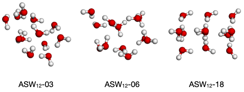
The ASW surface ice model was adapted from the “set-of-cluster" approach to obtain BE distributions using a similar methodology first introduced in [49] and [50]. We chose a cluster size of 12 water molecules to be able to use an accurate model chemistry for energies, gradients and Hessians, while at the same time having enough binding site diversity to obtain different binding modes and build a distribution of binding energies. To obtain the ASW surface model, a 12-molecule cluster was thermalised at 300 K using ab-initio molecular dynamics (MD) simulations at the BLYP/def2-SVP level of theory [51]–[54] to amorphise the system. From the high temperature trajectory, we selected 15 equally spaced frames and annealed the systems to 10 K. These 15 clusters of 12 water molecules each span the set-of-cluster model on which we sampled from binding sites. Figure 1 shows three representative water-ice clusters for illustration.

2.1 Computational framework↩︎

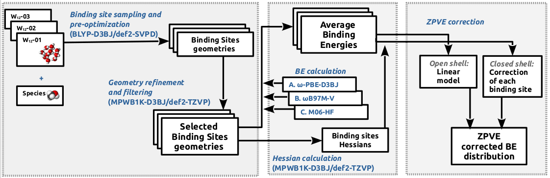
The BEEP (Binding Energy Evaluation Platform) framework was utilised in this study, as first described in [40]. The construction of the BE distributions on a set-of-clusters model follows a structured three-step procedure: i) sampling and geometry refinement, ii) binding energy and Hessian computation, and iii) ZPVE (zero-point vibrational energy) corrected BE distribution assembly. Figure 2 shows a schematic diagram of the three workflows. We used BEEP v0.6.0 for this study. The BEEP source code is publicly available¹.

2.1.1 Levels of theory↩︎

Initial geometry optimisations for methanol and other closed-shell or stable species were performed at the BLYP-D3BJ/def2-SVPD [55]–[57] level of theory with Grimme’s D3-BJ dispersion correction [58]. For radical species, we employed unrestricted BLYP calculations [55], [56], [58] using the same basis set and dispersion correction. We chose this level as it provides good initial geometries from the sampling round for further refinement.

After sampling, we refined these structures using MPWB1K-D3BJ/def2-TZVP [58]–[60] for closed-shell species and UMPWB1K/def2-TZVP-D3BJ [58]–[60] for open-shell (i.e., radical) systems. All DFT computations where done with Psi4 quantum chemistry software² and the empirical dispersion correction was computed with dftd3 package.

2.1.2 Binding energy formalism↩︎

The BE (\(\Delta E_\mathrm{b}\)) was obtained using a basis set superposition error [61] corrected electronic energy while also including the zero-point vibrational energy (ZPVE) contribution, \[\Delta E_\mathrm{b} = -(E_\mathrm{X + ice} - (E_\mathrm{X} + E_\mathrm{ice}) + \Delta_\mathrm{ZPVE}), \label{Equ:BEcomp}\tag{1}\] where X is the adsorbate species of interest. The negative sign in Eq. 1 is due to the convention of a positive definition of BE. \(\Delta_{ZPVE}\) is defined as \[\Delta_{ZPVE} = E_{ZPVE,X+\text{ice}} - (E_{ZPVE,X} + E_{ZPVE,\text{ice}}).\] In the case of open-shell molecules, the ZPVE corrected BEs where obtained by scaling the non-ZPVE corrected molecules by the linear models obtained by relating ZPVE-corrected BEs with BEs on a single water cluster (see Appendix 7).

2.1.3 Updated BEEP protocol↩︎

The BEEP protocol has recently been updated to incorporate additional refinements in the final BE calculation step. The final BE is calculated as an average across three distinct levels of theory. These levels of theory were validated using benchmarks on small water clusters with one to three water molecules. The detailed results of the benchmark are given in Appendix 8. Based on the benchmark results, the following levels of theory were chosen in this study for BE computation: \(\omega\)-PBE-D3BJ [62], [63], \(\omega\)B97X-V [64] and M06-HF [65] with the def2-TZVP [60] basis set. For the more weakly bound species, and , we employed XC (exchange-correlation) functionals that performed best in the benchmark. These were B97-2-D3BJ [63], [66], \(\omega\)B97M-V [67] and TPSSh-D3BJ [63], [68], with the same basis set. Overall, the standard deviation in the BEs computed using the three approaches was less than 200 K, which is comparable to the mean absolute error (MAE) of the different methods in the benchmark.

For all the binding sites of the closed-shell or stable molecules, we computed full Hessian matrices to determine the ZPVE corrections and filter structures with negative Hessian matrix eigenvalues. Due to the high computational cost of calculating all Hessians for open-shell species, we adopted a linear model approach for the ZPVE correction based on a limited set of Hessian calculations (see Appendix 7).

These ZPVE-corrected and BSSE-corrected BEs were then used to generate the final BE distribution for each ASW\(_{12}\)–X system, where X represents the adsorbate species under investigation.

3 Results↩︎

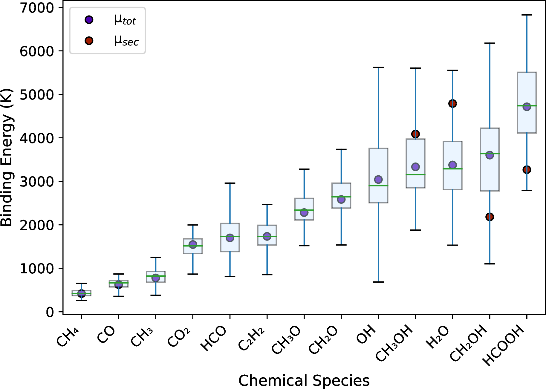
We calculated BE distributions for thirteen species including methanol and its related species on ASW\(_{12}\) clusters (see Fig. 3). Our analysis encompassed two molecular subsets; i) closed-shell or stable species (CO, , , , , HCOOH, , and ), and ii) open-shell radicals known to form through methanol photolysis (OH, , HCO, , and ). For each species, we characterised the average primary (\(\mu_\mathrm{tot}\)) and secondary (\(\mu_\mathrm{sec}\)) binding modes (if present) as illustrated in Figs. 4, 5, and 6. We compute the average binding energy (\(\mu_\mathrm{tot}\) or \(\mu_\mathrm{sec}\)) and its associated error (\(\sigma_\mathrm{tot}\) or \(\sigma_\mathrm{sec}\)) using Gaussian fits to the BE distributions using the same method as described in [40]. We provide the full list of computed BEs for each system (BE_lists.tgz), and all optimised structures (all_xyz.tgz), in tar archives attached to the paper. All datasets are also available on Zenodo ³.

Figures 3 and 5 reveal that volatile species such as CO and exhibit narrower BE distributions. This suggests that these species interact relatively weakly and uniformly with the surface, resulting in less variability across different adsorption sites. Less volatile species such as , and HCOOH show broader distributions, reflecting the presence of multiple binding environments, including sites capable of forming strong H-bonds (see Figs. 3 and 4). These trends highlight the importance of considering a range of BEs when modelling strongly interacting molecules on ASW ices. Building upon these general observations, we next examine the BEs of the closed-shell and open-shell species, highlighting site-specific interactions.

3.1 Closed-shell species↩︎

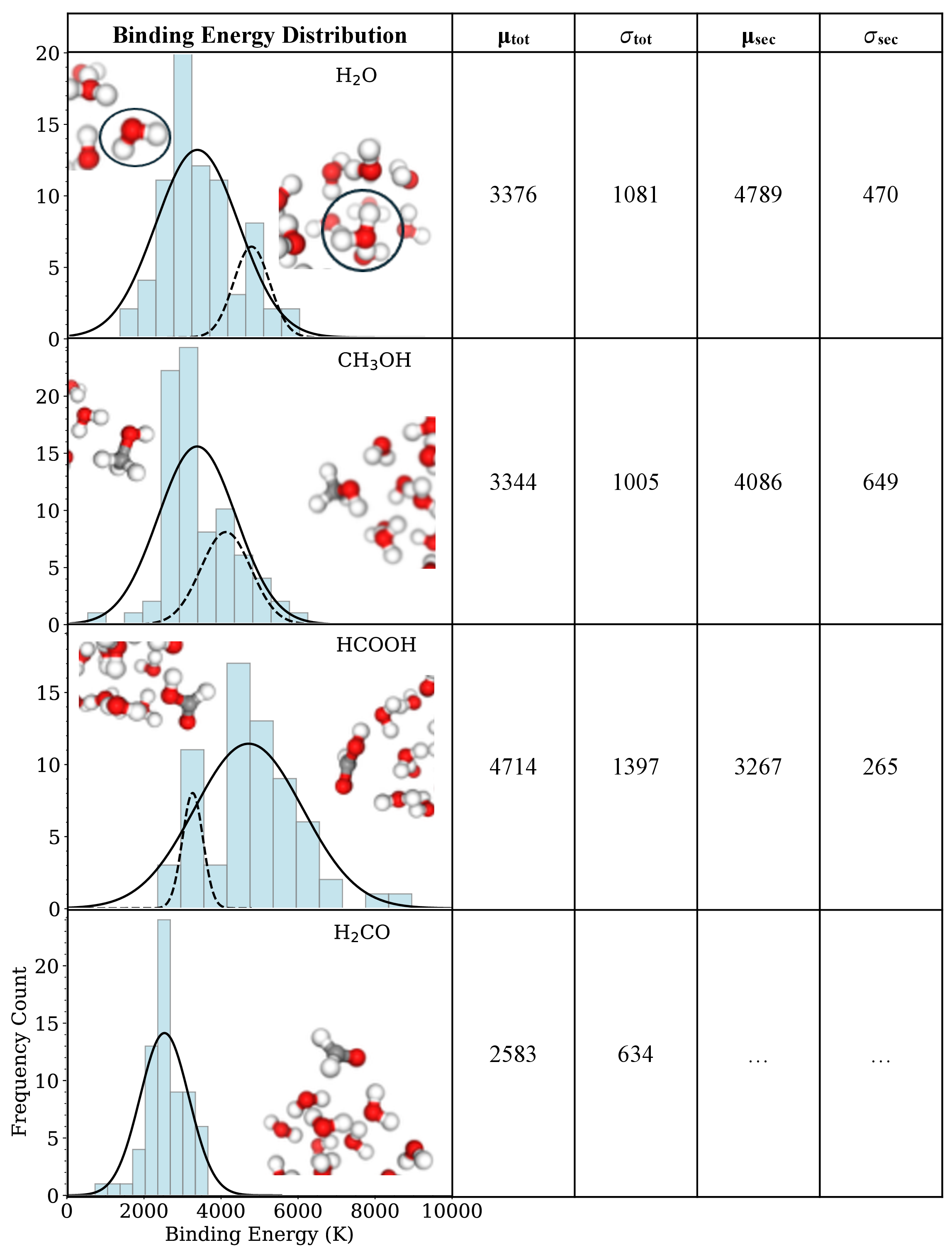
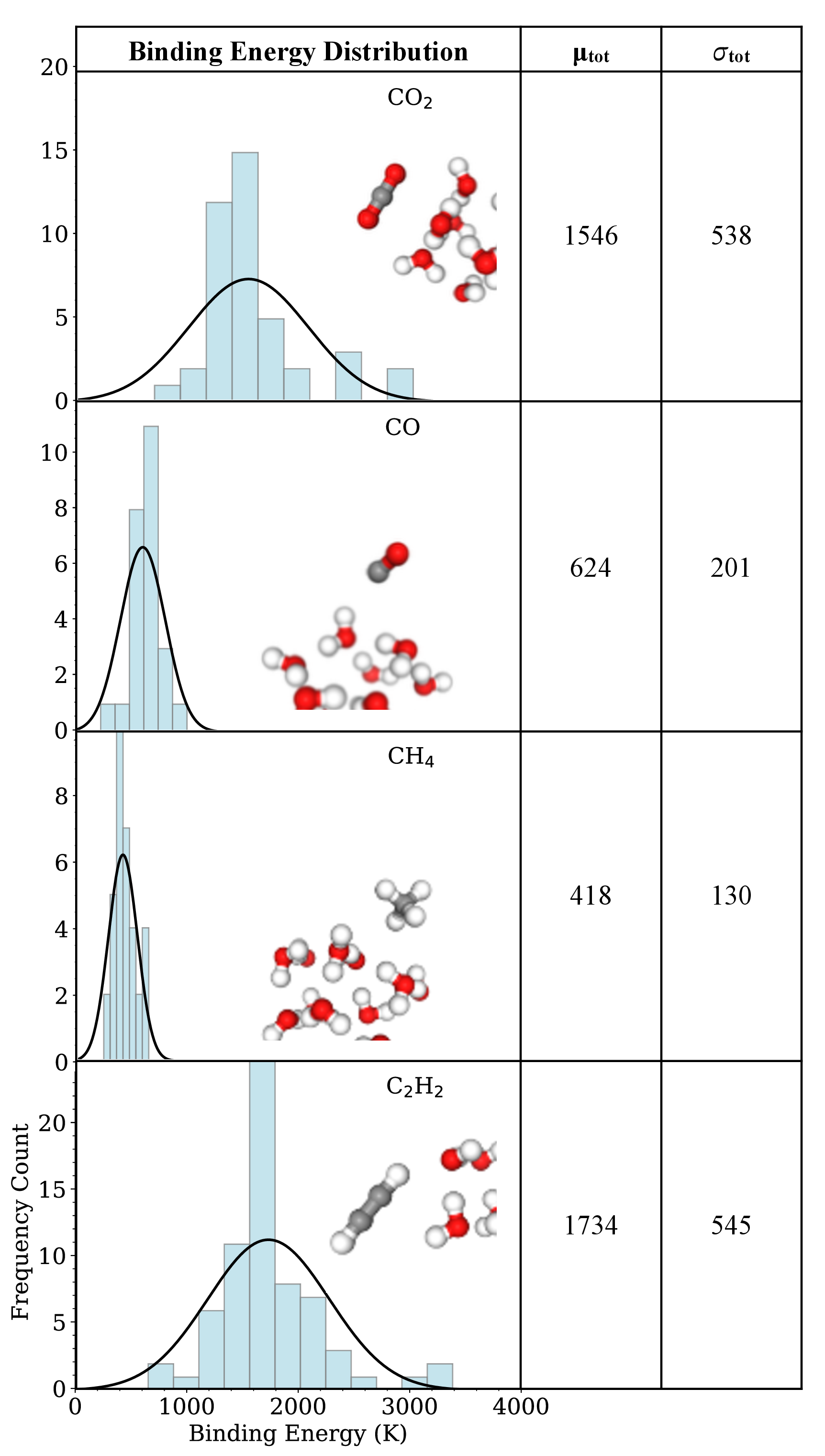
We calculated the BEs for eight closed-shell species which we divided into two groups. One group which have broad BE distributions sometimes with multiple binding modes (, , HCOOH, and ; see Fig. 4), and for which the primary mode of binding is through H-bonds. In the second group, dispersion interactions are significant for binding (, CO, , and ; see Fig. 5). For the species that have more than one binding mode, we report two values of the BE: \(\mu_\mathrm{tot}\) is the average binding energy computed from a Gaussian fit to the entire distribution which is dominated by the primary binding mode, and \(\mu_\mathrm{sec}\) is the value from a restricted fit over the secondary binding mode only. For species with a single binding mode, we report \(\mu_\mathrm{tot}\) only.

exhibits two distinct binding modes (see Fig. 4). The stronger secondary mode, \(\mu_\mathrm{sec}\) (\(4789\pm470\) K), corresponds to configurations where forms two H-bonds with the surface of the ASW\(_{12}\) clusters. The weaker primary mode, \(\mu_\mathrm{tot}\) (\(3376\pm1081\) K), reflects binding sites with dangling-OH (d-OH) configurations with reduced intermolecular contact with the surface of the cluster. This is in agreement with previous research that has also shown that the presence of d-OH groups can lead to weaker interactions with adsorbed species, resulting in lower BEs [69]–[72].

Similarly, also demonstrates two characteristic binding modes. The primary mode, \(\mu_\mathrm{tot}\) (\(3344\pm1005\) K), emerges when the moiety forms a single H-bond, and the moiety weakly interacts with the surface of the cluster. The secondary more stable bidentate binding mode, \(\mu_\mathrm{sec}\) (\(4086\pm649\) K), is a result of two strong H-bonds forming with the surface. Similar to , the weaker of the two binding modes for also involves d-OH groups, as shown in Fig. 4.

HCOOH was the final closed-shell or stable species that we determined to have two binding regimes. The stronger binding mode, \(\mu_\mathrm{tot}\) (\(4714\pm1397\) K), is a result of the formation of two H-bonds forming with the surface of the ASW\(_{12}\) clusters. HCOOH exhibits high BEs because it can both donate and accept hydrogen bonds via its OH and groups, thus resulting in a strong interaction of HCOOH with the clusters. The secondary mode, \(\mu_\mathrm{sec}\) (\(3267\pm265\) K), also forms two H-bonds with the surface of the clusters. However, the configuration is not parallel to the surface, resulting in a weaker surface interaction with HCOOH. The donor and acceptor behaviour of HCOOH is reflected in the broad distribution of BEs, highlighting the extended range of BEs for this adsorbate molecule.

Finally, exhibits only one peak in its BE distribution indicating the presence of a dominating binding mode in which the carbonyl oxygen receives a H-bond while the establishes an H-bond with a water oxygen acceptor. However, as has been shown in our previous work, the carbonyl oxygen can accept more than one H-bond thus increasing the binding energy with the surface [73].

The BE of the molecules in the second group is notably lower because they lack strong hydrogen bonding interactions with the water molecules on the cluster surface and are not considerably polarizable (see Fig. 5). with zero dipole moment and with a very small dipole moment (0.122 D) stand out as the molecules with the lowest BE due to the absence of polarization and therefore a significant portion of the BE is due to weak dispersion interactions. On the other hand which has a polarized electron density towards the oxygen atoms, and with a polarizable \(\pi\)-bond, display stronger binding to the water clusters. Due to the lack of H-bonds and a single binding motif, the molecules in this group display a single BE distribution.

3.2 Radicals↩︎

The BE values and distributions of open-shell radical species, namely , , OH, , and HCO are shown in Fig. 6. Open-shell species demonstrate binding characteristics distinct from those of their closed-shell counterparts as a result of the unpaired electron that alters their hydrogen-bonding patterns and preferred adsorption orientations.

The radical exhibits its primary interactions through its oxygen moiety, similar to ’s group, but with altered surface orientation. only accepts an H-bond due to the lack of an group, yielding an average BE of \(2281\pm610\) K, lower than the average BE for methanol (\(\mu_\mathrm{tot} = 3419\pm139\) K).

Amongst the radicals, is the only one that displays dual-binding behaviour, mediated by its OH moiety and radical carbon centre. This results in distinct binding modes with varying degrees of H-bond participation. The stronger binding mode, \(\mu_\mathrm{tot}\) (\(3602\pm1293\) K), has a strong interaction of its OH moiety with the ASW\(_{12}\) cluster surfaces. The secondary mode, \(\mu_\mathrm{sec}\) (\(2185\pm349\) K), has a d-OH bond resulting in a weaker overall interaction of the radical, similar to our findings for and . The slightly overall higher BE of than that of is due to the less bulky moiety compared to the methyl group in , that allows the radical species to interact more efficiently with the water molecules on the surface.

The OH radical demonstrates strong binding as it can versatilely insert itself into the water H-bond network, resulting in a high BE of \(3041\pm1145\) K. On the other hand, (\(778\pm251\) K) lacks strong H-bonding capabilities, interacting primarily through dispersion forces, producing BE behaviour reminiscent of its closed-shell analogue , but modified by the radical center that enables a slightly stronger interaction. The binding energy for the HCO radical is \(1699\pm572\) K, with binding predominantly occurring through an H-bond between the oxygen and the ASW surface. HCO binds noticeably weaker to the ASW surface compared to other O-bearing radicals, and forms a weaker H-bond to the surface. This might be due to the more linear geometry that hinders the establishment of an efficient donor-acceptor H-bond interaction with the surface.

These findings demonstrate that electronic structure modifications resulting from radical formation can significantly influence adsorption geometries and energetics.

4 Discussion↩︎

4.1 Comparison with reported experimental binding energies↩︎

To assess the consistency of our theoretically-calculated BEs, we contrast them with the datasets compiled by [38] and [74], as summarized in Table [tab:experimental95BEs], and illustrated in Figure 7. In Table [tab:experimental95BEs] we also show the uncertainty which arises from the choice of DFT functional (\(\sigma_\mathrm{comp}\)), and the BE for the strongest binding site identified for each species (\(BE_\mathrm{max}\)). In Fig. 7 we only plot data for which there are available experimental values.

[38] compiled experimentally determined BEs obtained primarily via TPD experiments, where BEs are derived from the data using the Polanyi-Wigner equation. These experimental values inherently reflect surface dependent effects such as sub-monolayer coverage, surface morphology, and heterogeneity in binding sites. In contrast, [74] compiled BEs from a mixture of experimental reports and theoretical estimates to be used in astrochemical gas-grain modelling to explore the sensitivity of model results on the assumed suite of BEs. Their work derives the BEs from TPD experiments where data are available, by scaling the binding energy relative to that for using the ratio of the desorption temperatures as measured from TPD curves.

The experimental BEs reported in Table [tab:experimental95BEs] and illustrated in Fig. 7 are, in general, larger than those derived from our theoretical calculations. For example, the average BE for in our simulations is \(3376\) K, whereas the experimentally reported values range between 4800–5930 K (see references listed in Table [tab:experimental95BEs]).

Surface morphology and coverage contribute significantly to the observed differences. As an example, experiments by [75] measuring the thermal desorption of and CO from a sub-monolayer mixture reveal that, under sub-monolayer conditions, molecules preferentially occupy the strongest available binding sites, which in turn leads to a TPD peak that is shifted to higher temperatures and consequently a higher BE [76], [77]. We also list the binding energies for the strongest binding sites, \(BE_\mathrm{max}\), identified in our calculated distributions. In some cases the strongest identified binding sites lies closer to those derived from TPD experiments (e.g., CO and ) than the peak value we derived from a Gaussian fit to the data (\(\mu_\mathrm{tot}\)). For most species, however, the strongest binding site is significantly larger than the values derived from experiment. This is most notable for the species for which H-bonds play an important role in the binding (e.g., , , HCOOH, , and OH).

The discrepancies between our results and experimental data are particularly pronounced for volatile species like CO and , consistent with the difficulty of accurately probing weak physisorption interactions in experiments. However, these weak interactions could play an important role in the desorption and diffusion patterns of volatiles species in cold interstellar environments [39]. Conversely, for strongly-bound species such as the OH radical and HCOOH, our calculated BEs show better agreement with the experimental determinations. These findings emphasise the importance of accounting for surface heterogeneity when interpreting BEs derived from laboratory measurements, and they highlight the complementary role of theoretical modelling in advancing our understanding of grain-surface interactions and chemistry.

4.2 Comparison with reported theoretical binding energies↩︎

Our study adopts the BEEP protocol, following the approach outlined by [40]. Similar to [40], we explore the distribution of BEs by examining all unique adsorption sites on a set of water clusters; however, our use of a set of ASW\(_{12}\) clusters (as opposed to ASW\(_{22}\)) and our multi-level DFT approach (e.g., WPBE-D3BJ, \(\omega\)B97X-V, M06-HF) introduce some differences in the final calculated BEs. Figure 8 visualises the impact of the methodological differences of our theoretically-calculated BEs to the literature. Since the set-of-clusters model ASW explicitly accounts for the diversity of binding sites accessible on the surface, it is not surprising that our distributions encompass the range of theoretical values reported in previous studies.

Table [tab:theoretical95BEs] shows how our computed values compare to [40]. In general the values fall within the range of our BE distributions; however the mean values are marginally different due to both the different cluster size, and the more refined level of theory employed in this study. For the volatiles, the discrepancies are larger due to the lack of application of the ZPVE correction in data presented in [40]. Comparison of the non-ZPVE-corrected binding energies reveals the effect of cluster size, particularly for CO, for which binding energy distribution data are available at comparable DFT levels of theory. Here we report an average BE of 930 K. When using a 22-water molecule cluster as in [40] the average value increases to 1030 K using the M05-2x/def2-tzvp level of theory for the binding site optimization and \(\omega\)-PBE-D3BJ/def2-tzvp for the BSSE corrected BEs, reflecting a 10% increase in the average BE value. In [78] the same CO BE distribution was computed using a machine learning potential (trained on MPwB1K-D3BJ/def-tzvp level of theory) on several large 500 water molecule surfaces. This very realistic surface provided an average BE of 1350 K again increasing the BE relative to the smaller cluster systems. We expect that a similar model size effect will be also observed for other molecules like and . Even though the average BE values stemming from the distribution on ASW\(_{12}\) clusters using the set-of-clusters approach provides a systematically lower BE values than larger systems, it still samples the same binding modes that one can find on the more realistic surface providing accurate relative BEs among the species in this study and for the employed surface model.

Other variations stemming from cluster shape and sampling strategies become evident when comparing our results with those of [46] and [47] who used a similar ASW model. In particular, [46] examined up to eight binding sites per species on a periodic amorphous solid water (ASW) slab of 60 water molecules. Their larger and continuous ice representation yielded in average higher BEs, likely due several binding sites being in a cavity resulting in the interaction with a greater number of water molecules, and a better representation of H-bond cooperativity effects in the larger system. In contrast, our sampling procedure explores all unique binding sites, thus capturing the heterogeneity of binding configurations leading to our reported \(\mu_\mathrm{tot}\) and \(\mu_\mathrm{sec}\) values that effectively encompass both weaker and stronger interactions.

Methodological choices also play a key role in reported discrepancies. High-level quantum chemical techniques, such as the CCSD(T) [79] approach employed by [42] for small water clusters (N= 1-4), often yield benchmark-level accuracy for specific configurations. However, their high computational cost limits the number of adsorbates and binding sites that can be treated, possibly overlooking broader site variability effects. Our dispersion-corrected DFT approach mitigates this limitation by enabling the treatment of larger ASW\(_{12}\) clusters while still accounting for dispersion effects. As a result, our BEs for larger or strongly H-bound species, like HCOOH, depart substantially from smaller-cluster CCSD(T) values (e.g., 4714 K and 3267 K versus 1479 K reported by [42]), but capture bidentate H-bonding motifs more comprehensively.

Studies by [48] and [41] further highlight how differences in cluster size, ice morphology, and computational methods influence the calculated BEs of interstellar species on water ices. [48] report significantly higher BEs for OH (4287 K) compared to our mean value of 3041 K, partly due to their use of a larger ASW\(_{20}\) cluster. However, their BE distribution appears to be derived from a targeted selection of high-binding-energy sites, potentially introducing a sampling bias that over-represents strong adsorption environments. In contrast, our BEEP approach samples the surface more uniformly, yielding a broader and more physically representative distribution of BEs. Meanwhile, [41] report over- or under-estimations relative to ours, which can be attributed to the consideration of a single binding site for their study. On the other hand, the values reported by [45] are systematically higher than our results, as they are derived from a linear model that related BEs computed on water monomer to experimental TPD BE values.

Recently [39] obtained a full BE distribution for on a large 200 water molecule cluster that includes several concave regions using ONIOM⁴ embedding methods. They obtained a mean value of 4255 K for the BE of which is 800 K higher than the value reported here. The spread in the BE values is also 500 K wider than the one obtained in this study. This is expected for molecules that can form multiple hydrogen bonds to the ASW surface since the presence of nano-pores in larger clusters can enhance the strength of the hydrogen bonding and hence the BE.

4.3 Comparison with data collated by the UMIST database↩︎

Our results can also be placed in the context of widely used astrochemical databases such as the UMIST Database for Astrochemistry [81] which compiled BEs from a mix of experimental data, older theoretical calculations, and empirical estimates. While these databases provide essential inputs for astrochemical modelling, their values often lack the uniform level of refinement that comes from a single, high-level protocol such as the approach highlighted in BEEP.

For instance, our two binding regimes for (\(\mu_\mathrm{tot} = 3376\) K and \(\mu_\mathrm{sec} = 4789\) K) lie below the UMIST (4800 K) value. Similar patterns emerge for , where our bidentate H-bonding results (3344 K and 4086 K) are lower than the 4930 K value listed in UMIST. The differences are particularly pronounced for weaker adsorbates like CO, where our low BE (624 K) contrasts with that compiled by UMIST (1150 K). Taking a set of binding energies from disparate sources (i.e., a mixture of theoretical and experimental data) that follow different methodologies and experimental design will generate a set of binding energies not fully consistent with each other. What likely matters most for grain-surface chemistry are the relative binding energies of species which are competitors in grain-surface reactions, and those which are important for setting the locations of snowlines. The approach adopted here allows such a set of binding energies to be determined.

5 Astrochemical modelling↩︎

To test the impact of using a consistently-derived suite of binding energies in an astrochemical model, we simulate the chemistry of a dark cloud with a temperature of 10 K (for both gas and dust), an number density of \(10^{4}\) cm\(^{-3}\), a visual extinction of 10 magnitudes, and a cosmic-ray ionisation rate of \(1.3\times 10^{-17}\) s\(^{-1}\). We use the chemical network and model from [82] and adopt initial elemental abundances from [81].

The BE is used in the model in two ways. Firstly, for the thermal desorption rate, \(k_\mathrm{des}\), \[k_\mathrm{des} = \nu \exp\left(\frac{-\Delta E_b}{T}\right),\] where the BE (\(\Delta E_b\)) is in units of K and \(\nu\) is the characteristic frequency of the bound species, often also referred to as the “pre-exponential factor". The BE is also used to estimate the size of the barrier to hopping, and hence controls the rate of diffusion of ice species across the surface, and by extension, the grain-surface reaction rates. The rate of thermal hopping, \(k_\mathrm{hop}\), is similarly \[k_\mathrm{hop} = \nu \exp\left(\frac{-\chi \Delta E_b}{T}\right),\] where \(\chi\) is a scaling factor that sets the ratio of the barrier to diffusion to that for desorption. Lower values of \(\chi\) are typically assumed for diffusion across the ice surface (\(0.3 - 0.5\)), whereas higher values (\(\approx 0.7\)) are assumed for diffusion of molecules within the bulk ice mantle in so-called three-phase models, in which the chemistry in the mantle is computed separately from that on the surface [43], [83]. Here, we run a two-phase gas-grain chemical model (i.e., assuming that chemistry occurs on the ice surface only) where we include a large gas-phase network (the base for which is Rate12; [81]), freeze-out, thermal desorption, photodesorption (driven by cosmic-ray-induced UV), reactive desorption (with an efficiency of 1%), two-body grain-surface reactions (via the Langmuir-Hinshelwood mechanism), and ice photodissociation (driven by cosmic-ray-induced UV). The ratio of the barrier to diffusion to that for desorption is an uncertain parameter not yet well constrained by experiment nor theory, except in a handful of cases (see the discussions in [83] and [84]). To explore the effects on the results on the assumed ratio for the barrier to diffusion to that of desorption, \(\chi\), we run models using a value of 0.3 (faster diffusion) and 0.5 (slower diffusion). We note here that the diffusion of H and is controlled solely by quantum tunnelling at 10 K [85]; hence, the rates of H and diffusion is the same across all models.

We run models adopting different sets of BEs. The first is one in which we use the BEs for the species of interest here as compiled by the Rate12 version of the UMIST Database for Astrochemistry (see Table [tab:experimental95BEs]) and for which we adopt the harmonic oscillator approximation to compute the pre-exponential factor, \(\nu\) [86], \[\nu_\mathrm{HO} = \sqrt{\frac{2\,n_s k_{B}\Delta E_b}{\pi^2 m}}, \label{equ:HO}\tag{2}\] where \(n_s\) is the number density of surface sites, \(k_{B}\) is Boltzmann’s constant, \(\Delta E_b\) is the BE in units of K, and \(m\) is the mass of the bound species. This equation typically gives values of the order of \(10^{12}\) s\(^{-1}\) for all species.

In a second model, we replace the binding energies of the species of interest here with those derived from the fit to our BE distributions (\(\mu_\mathrm{tot}\)) and we recalculate the pre-exponential factor, \(\nu_\mathrm{TST}\), using transition state theory (TST). As outlined in [38], \[\nu_\mathrm{TST} = \frac{k_{B}T}{h}q_\mathrm{tran,2D}q_\mathrm{rot,3D}, \label{equ:TST}\tag{3}\] where \(h\) is Planck’s constant and \(q_\mathrm{tran,2D}\) and \(q_\mathrm{rot,3D}\) are the 2D translational and 3D rotational partition functions for an adsorbed species, respectively [38].

In the computation of \(\nu\) using TST, the moments of inertia, \(I_x\), of the adsorbed species are required and we compute them in this work for geometries optimized at the MPWB1K-D3BJ/def2-tzvp level of theory. In Table [tab:Iandnu] we list the symmetry numbers and moments of inertia for each species, as well as a comparison of the characteristic frequencies computed using the harmonic oscillator approximation, \(\nu_\mathrm{HO}\) (Eq. 2 ), and those computed using transition state theory, \(\nu_\mathrm{TST}\) (Eq. 3 ), at a temperature of 10 K which is that assumed in our chemical model. In these calculations, and in the chemical model, we assume a number density of surface sites of \(6\times10^{14}\) cm\(^{-2}\). For some species, \(\nu_\mathrm{TST}\) is slightly lower than or similar to \(\nu_\mathrm{HO}\) which is the case for , OH, , and ; however, for most species, \(\nu_\mathrm{TST}\) is around 1 to 2 orders of magnitude larger. For these species, the thermal desorption rates and thermal hopping rates will be faster, compared with those computed using the harmonic oscillator approximation which is traditionally assumed in astrochemical models [38].

Figures 9 and 10 show the results from a single-point model of a dark cloud using the BEs for the species considered here from those compiled by the UMIST database in dashed lines (“UMIST”), and those from our calculations, including calculating the pre-exponential factor using transition state theory, in solid lines (“BEEP”). We plot the fractional abundances for all species considered here in both the gas (Fig. 9) and ice (Fig. 10) phase, for two values of \(\chi\), the ratio of the barrier to diffusion to that for desorption (\(\chi=0.3\) and 0.5 in the left- and right-hand panels, respectively). We also plot the fractional abundances of larger complex organic species which have been postulated to be directly formed from the radicals we consider in this work, and thus are chemically related to methanol [12].

For closed-shell stable species we see only small differences in their gas-phase abundances comparing the results from both approaches. For instance, the results for water gas and ice are almost identical regardless of the assumed BEs and the adopted value for \(\chi\) [83]. This is because in our model, water ice formation is dependent on the rate of hydrogenation via quantum tunnelling. We see a slight decrease and increase by a factor of a few in gas-phase and at late times (\(\gtrsim 10^5\) yrs), respectively, when using the BEEP values for both values of \(\chi\). There is also an increase in the abundance of gas-phase by around one to two orders of magnitude (between \(\sim 10^{5}\) and \(\sim 10^{7}\) yrs when \(\chi=0.3\)), and an increase in the abundance of by a factor of a few beyond a few times \(10^{5}\) years. The BEEP model assuming slower diffusion (\(\chi =0.5\)) predicts a noticeably higher gas-phase abundance, reaching a peak of a few times \(10^{-5}\) with respect to . Regarding the gas-phase radical species, the abundances of OH gas and ice are practically identical in all models and there are only small differences for the gas-phase abundances of and HCO over the full model timescale when comparing the UMIST results with the BEEP results. For the slower diffusion model (\(\chi=0.5\)), the abundance of gas-phase and decrease and increase respectively, compared with the faster diffusion model (\(\chi=0.3\)). The abundance of gas-phase is higher by a factor of a few just beyond \(10^{6}\) yrs when using the BEEP approach for both values of \(\chi\). The abundance of gas-phase is more sensitive to the assumed diffusion barrier. Its abundance is lower by up to two orders of magnitude in the BEEP model than those computed using the UMIST values when \(\chi=0.3\); however, when diffusion is assumed to be slower, the differences between the BEEP and UMIST models are more minor.

There is a lot more variation between the models for the large complex organic molecules (COMs). These species are generally only formed efficiently on the grain surfaces and are released into the gas phase via non-thermal desorption. A key difference between the models with fast (\(\chi=0.3\)) and slow (\(\chi=0.5\)) diffusion is the absence of methyl formate (), glycol aldehyde () and ethylene glycol () in the gas phase when diffusion is slow, indicating the sensitivity of the formation rate of these species to the assumed diffusion rate. In the fast diffusion case, the BEEP model predicts a lower abundance of ethylene glycol (), glycolaldehyde (), and methyl formate (), and slightly more dimethyl ether (), in the gas phase. Both model approaches predict similar abundances of gas-phase acetaldehyde, , suggesting the importance of gas-phase chemistry in setting its abundance. The decrease in -containing species is likely due to the higher binding energy adopted in the BEEP approach. For the -containing species, this radical is less weakly bound, and thus more mobile, and there is a competition between radical-radical recombination with hydrogenation to reform . In the slow diffusion model, the BEEP approach generally predicts a higher abundance of and than when using the UMIST approach, with the abundance of in the BEEP model higher by between one and two orders of magnitude.

For the ice species (Fig. 10), in general, the BEEP approach predicts higher abundances of , , , CO, and when diffusion is fast. When diffusion is slow, the picture is more complex. The rates of formation of the ice species differ when using both approaches (indicated by the gradient); however, similar abundances of , , , CO, and are reached between \(\sim 10^{5} - 10^{7}\) years. The BEEP approach predicts a significantly lower abundance of ice regardless of the assumed barrier to diffusion, indicating increased competition between those species formed via reactions with CO on the ice surface.

Similarly, for the fast diffusion case, the BEEP approach generally predicts higher abundances of radicals in the ice phase, with the exception of which has negligible abundances over the whole timescale (\(\lesssim 10^{-13}\)). This could be due to the lower binding energy for predicted in this work which will increase its hopping and desorption rates and thus reduce its residency time on the grain. When diffusion is slow, the rates of formation of the radicals on the ice is faster (i.e., traced by the steeper increase in the abundance with time), when using the BEEP approach; however, again, similar abundances of HCO, , and are obtained between \(\sim 10^{5} - 10^{7}\) years. is the exception here once again, with the UMIST model predicting a significantly higher abundance in the ice (reaching a peak of \(\sim 10^{-5}\)) versus that in the BEEP model (\(\lesssim 10^{-8}\)).

For the COMs, the ice abundances mimic those in the gas phase in the fast diffusion case, with , , and having less efficient formation, and and having slightly more efficient formation. These latter two species can be formed from association reactions involving the radical, and their synthesis could be increased in efficiency by the increased mobility of this species on the ice surface. For the slow diffusion case, only and are efficiently formed in the ice phase, with the BEEP model predicting higher abundances than the UMIST model. The assumption of slow diffusion suppresses the formation of and in both models. The disappearance of methyl formate (), glycolaldehyde (), and ethylene glycol () in the slow-diffusion model indicates that the predicted abundances of these species are highly sensitive to the adopted diffusion-to-binding energy ratio, \(\chi\). This highlights the need, in future work, to compute or constrain species-specific diffusion barriers, or distributions of diffusion barriers on realistic ice surfaces, rather than relying only on a fixed fraction of the binding energy.

We discuss here some caveats to our modelling approach. Firstly, we use a two-phase model so that we do not distinguish fully the chemistry occurring in the bulk ice from that occurring in the surface. However, we do mediate the surface diffusion and reaction rates by allowing only two monolayers of ice to be chemically “active". Nonetheless, use of a three-phase or multi-phase gas-grain chemical model may mute somewhat the differences seen here between the slow and fast diffusion models. Further, the models that we have run are not fully internally consistent in the approach to computing the thermal desorption and hopping rates. We recompute these only for the species considered here, and adopt the traditional approach (i.e., assuming harmonic oscillator) for all other species in the network. Hence, these models should be treated only as illustrative of the differences that can be expected when using a more appropriate approach for a sub-set of species in the network and we make no judgement on the accuracy of the model results when compared with, for example, observations of interstellar ices.

6 Conclusions↩︎

In this work, we have provided an accurate and self-consistent ab initio set of BE distributions for 13 methanol and methanol-derived closed- and open-shell species adsorbed on ASW, to be used in astrochemical models. Using an improved BEEP protocol applied to the set-of-cluster ASW\(_{12}\) model, we used multiple curated DFT functionals for the calculation of BEs which put together yielded a BE distribution for each species. All binding sites geometries were obtained at the DFT level of theory paired with large basis sets; ZPVE corrections were included for all BEs resulting in highly accurate values for the employed model surface.

Species, such as , , HCOOH, and OH, exhibit broader BE distributions, attributed to their ability to form multiple H-bonds with the ice surface. In contrast, volatile and weakly interacting species such as CO, , , and display narrower distributions. H-bonding leads to higher BEs, particularly for molecules possessing donor and acceptor functional groups (e.g., and ). We also obtained DFT level BE distributions for key radicals for surface chemistry such as , , HCO, and OH, with the and OH radicals exhibiting the highest BE amongst open-shell species due to their strong H-bonding capabilities and compact form that allows for a more efficient interaction with the surface water molecules. Furthermore, CH\({_3}\)O and CH\({_2}\)OH radicals showed binding characteristics reminiscent of their methanol parent molecule, whereas HCO and CH\({_3}\), with limited H-bonding ability, had weaker BEs.

We used the BEs computed here in conjunction with the recalculation of the pre-exponential factors, \(\nu\), using transition state theory, in a single-point chemical model of a dark cloud. We compared the results with a model in which we use the UMIST binding energies and calculate \(\nu\) using the harmonic oscillator approximation and assumed two different values for the ratio of the barrier for diffusion to that for desorption. The abundances of both and OH are very similar when using either approach, and there is a slightly increased efficiency in ice-phase and formation when using the BEEP values for the case of fast diffusion. The BEEP approach with fast diffusion also showed less efficient synthesis of -containing ice species such as and , and more efficient synthesis of -containing ice species such as and . There were several extreme responses in the chemistry, including a drop in the abundance of both and in the ice in the BEEP models, as well as in both phases. Further, the formation of and ice and gas were suppressed when diffusion was assumed to be slow in both models. This indicates that the chemistry, even at a low temperature of 10 K, is sensitive to the assumed BEs and to the method used to compute the characteristic frequencies. These results highlight the need for BE calculations for all ice species present in astrochemical networks to produce a self-consistent suite of data.

Our findings highlight the importance of incorporating realistic BEs into astrochemical models, particularly for species with strong surface interactions, and for radicals which are poorly constrained experimentally. Future work will extend these results to a larger range of species, and to the predictions of BEs for mixed ASW-methanol clusters and will introduce the binding behaviours of ice clusters.

7 ZPVE Models↩︎

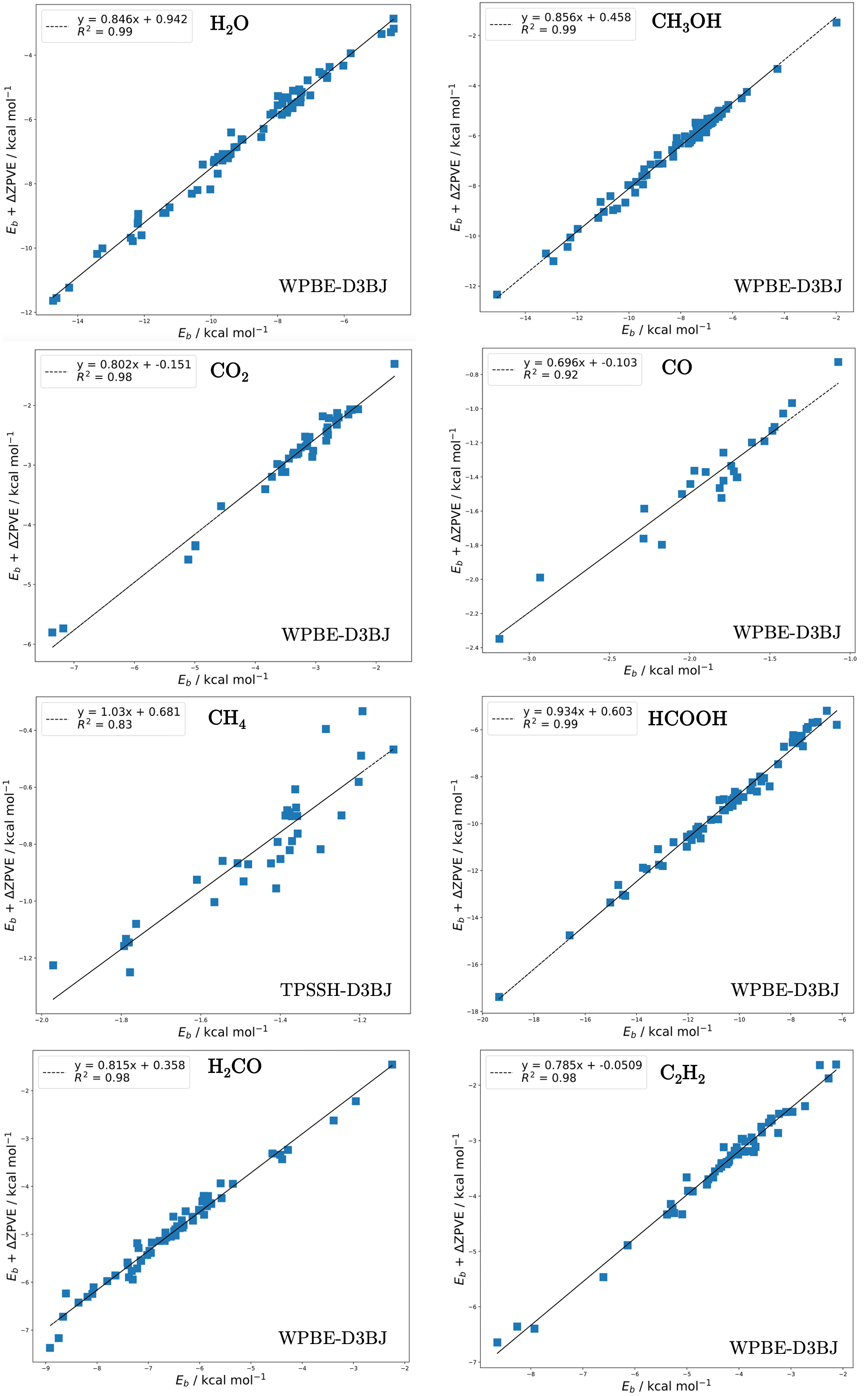
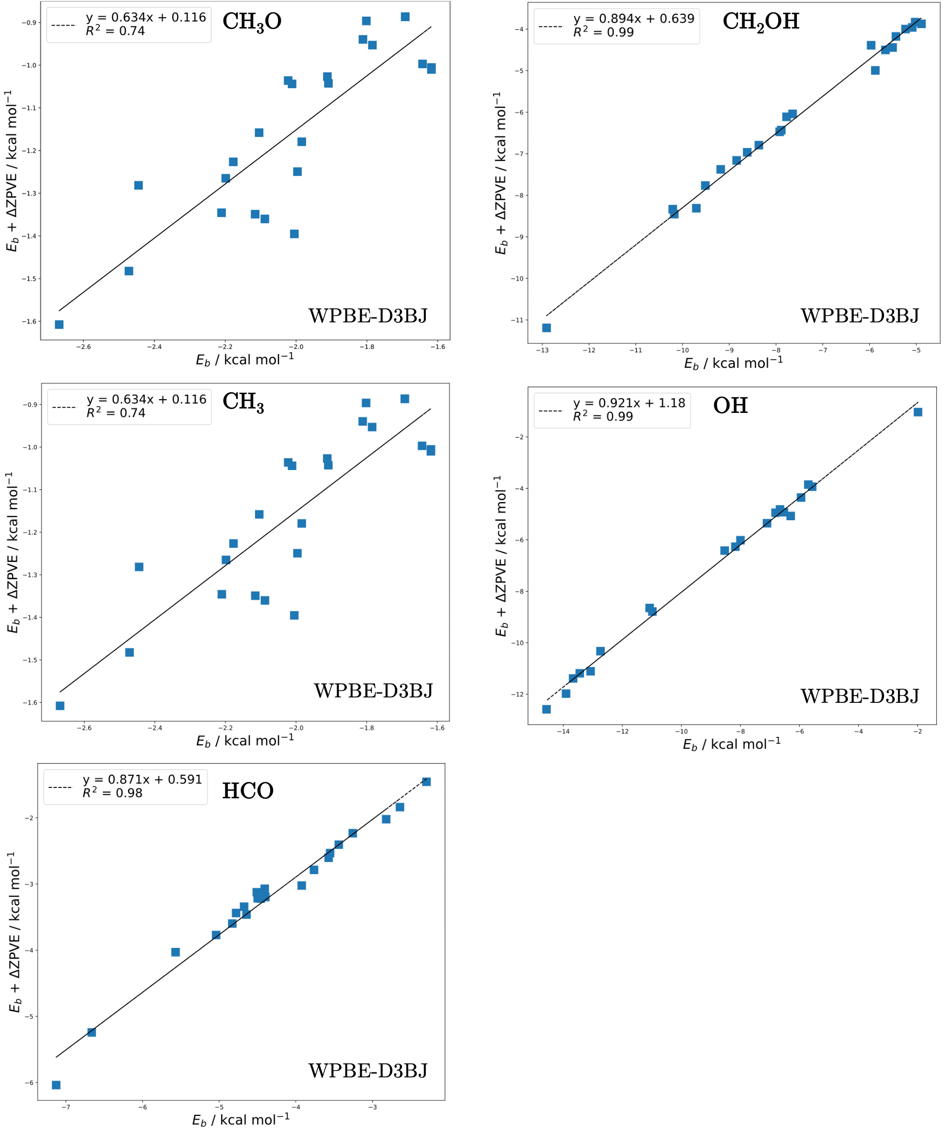
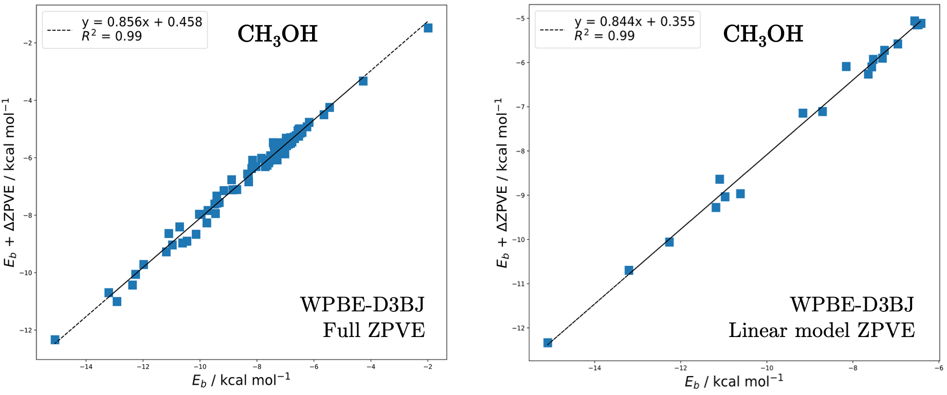
In Figs. 11, 12, and 13, we show the zero-point vibrational energy (ZPVE) for the closed shell molecules and radicals studied in this work. The ZPVE linear model was only applied to the radical species for which the Hessian computation on all binding sites was prohibitive. Of those, , and showed the poorest fit; however the uncertainty from the fit of the ZPVE is between 0.15 and 0.2 kcal/mol so within the error of the DFT methodology. Finally, we evaluated how much the ZPVE linear model changes using all binding sites versus using the binding sites that are contained only on one ASW cluster. The linear fit is very similar in both cases, thus confirming that building a linear fit with the binding sites on one cluster for the radical species is a good approximation.

8 DFT Binding energy benchmark↩︎

To determine a high quality model chemistry for binding energies, we benchmarked 128 exchange–correlation functionals against reference CCSD(T)/CBS energies. The benchmark set comprises 17 cluster configurations across six molecules: , , , , , and , with one to three water molecules in each cluster. The reference energies were obtained at the CCSD(T)/CBS level using the focal-point approach with Dunning’s augmented correlation-consistent basis sets (aug-cc-pVXZ). The Hartree–Fock energy and MP2 correlation energy were extrapolated to the complete basis set limit using cardinal numbers X = D, T, Q, while the CCSD(T) correlation contributions were extrapolated using X = D, T. All DFT single-point energies were computed on MPWB1K-D3BJ/def2-TZVP optimized geometries using the def2-TZVP basis set. Open-shell species ( and ) were treated with unrestricted Kohn–Sham (UKS).

Table [tab:BE95closed] presents the top 15 functionals ranked by mean absolute error (MAE) for closed-shell species (excluding ). Tables [tab:BE95ch4] and [tab:BE95uks] report the rankings for –water clusters and open-shell species, respectively.

In small cluster systems there are minimal cooperative H-bond effects, however on the target ASW\(_{12}\) set-of-clusters, cooperative many-body polarization and long-range electrostatic effects play a significant role. Therefore we selected three functionals from the closed-shell ranking (Table [tab:BE95closed]) that represent complementary physical approximations. \(\omega\)PBE-D3BJ is a range-separated hybrid that partitions exchange into short-range semi-local and long-range Hartree–Fock components. The D3BJ empirical dispersion correction provides an accurate and computationally inexpensive treatment of dispersion interactions. This functional offers a balanced description of both hydrogen bonding and dispersion at moderate cost. \(\omega\)B97X-V, a range-separated hybrid with the VV10 non-local correlation functional, was fitted self-consistently into the parameterization. Unlike the empirical D3 correction, the VV10 kernel captures dispersion through the electron density itself, providing a more physically motivated treatment of non-local correlation effects that become increasingly important in extended hydrogen-bond networks. Finally, M06-HF is a meta-GGA hybrid with 100% Hartree–Fock exchange. While M06-2X performs slightly better on the small benchmark clusters, M06-HF was selected for the larger set-of-clusters because full exact exchange eliminates the delocalization error inherent in semi-local exchange, which accumulates across the cooperative hydrogen-bond network of larger water clusters. Together, these three functionals span the dominant sources of error in DFT descriptions of non-covalent interactions: short- versus long-range exchange partitioning (\(\omega\)PBE-D3BJ), density-based versus empirical dispersion (\(\omega\)B97X-V versus \(\omega\)PBE-D3BJ), and delocalization error (M06-HF). Any systematic deviation shared by all three is unlikely to arise from a single methodological artifact, strengthening confidence in the resulting binding energies for the ASW\(_{12}\) water clusters.

References↩︎