Complementing Emerson-Lei Elevator Automata (Technical Report)
June 25, 2026
Abstract
Büchi elevator automata naturally appear in several areas of formal methods as a structural expressibly-equivalent subclass of Büchi automata where every strongly connected component is either deterministic or inherently weak. It was shown that this class contains the majority of Büchi automata generated in practical applications, including LTL model-checking and verification of hyperproperties. Moreover, the elevator subclass enables more efficient complementation and determinization algorithms than unrestricted Büchi automata. In this paper, we introduce Emerson-Lei elevator automata, which is a generalization of Büchi elevator automata to richer acceptance conditions. We provide a complementation algorithm with a significantly better asymptotic complexity than the best known algorithm for unrestricted Emerson-Lei automata. The practical efficiency of our algorithm is demonstrated by an experimental comparison with the popular state-of-the-art tool Spot. Our work is, to the best of our knowledge, the first step towards practical algorithms for complementing, determinizing, and testing universality and inclusion of Emerson-Lei automata with rich acceptance conditions.
1 Introduction↩︎
The fundamental framework of automata on infinite words (\(\omega\)-automata)—such as Büchi automata (BAs), Rabin automata, or parity automata—has proven successful for verifying software properties [1]–[5]. Complementation of these automata is an operation used to analyze program termination [4], model-check temporal logics (e.g., QPTL [6], HyperLTL [7]), and decide logics (e.g., S1S [8], or fragments of first-order logic over Sturmian words [9]). Moreover, it is the underlying operation for determining whether the language of one \(\omega\)-automaton is included in, or equivalent to, that of another. Yet, in the general case, complementation is notoriously challenging, and its difficulty has led the verification community to consider automata with structural restrictions, which allow more efficient algorithms. Elevator automata are BAs whose maximal strongly connected components (SCCs) are all deterministic or inherently weak (i.e., all runs staying in the SCC are either accepting or rejecting). This subclass was first identified in [10] as a generalization of the well-known semi-deterministic (a.k.a.limit-deterministic) automata [11]. Recent work [12] showed that the vast majority of BAs considered in practical applications, e.g., LTL model checking and verification of hyperproperties, are elevator automata.
Orthogonally, LTL model checking, synthesis, and other applications have raised interest in more sophisticated types of automata. Many types of \(\omega\)-automata differ exclusively in their acceptance conditions [13]. The most general considered is that of Emerson-Lei automata (ELAs) [14], whose acceptance condition is an arbitrary Boolean combination of \(\mathsf{Fin}\) and \(\mathsf{Inf}\) predicates. The predicate \(\mathsf{Fin}(\tikz[baseline=-.33em]\pic{cacc={7}{\upshape c}};)\) denotes that all transitions labeled with the color \(\tikz[baseline=-.33em]\pic{cacc={7}{\upshape c}};\) occur only finitely often along an accepting run. Dually, \(\mathsf{Inf}(\tikz[baseline=-.33em]\pic{cacc={7}{\upshape c}};)\) denotes that some transition labeled with \(\tikz[baseline=-.33em]\pic{cacc={7}{\upshape c}};\) occurs infinitely often. For instance, BAs admit a single color \(\tikz[baseline=-.33em]\pic{acc=0};\), and their acceptance condition is \(\mathsf{Inf}(\tikz[baseline=-.33em]\pic{acc=0};)\). The main motivation for using more complex acceptance conditions is the succinctness of the automaton representation. For instance, ELAs are exponentially more concise than BAs [15]. Another motivation is algorithmic flexibility and operational costs. It is well known that BAs are not closed under determinization, whereas ELAs are; however, checking emptiness for ELAs is NP-complete, while it is in P for BAs [13].
Generalized Rabin automata (GRAs), whose acceptance condition is \(\bigvee_i \mathsf{Fin}(\tikz[baseline=-.33em]\pic{acc=0};_i) \land \mathsf{Inf}(\tikz[baseline=-.33em]\pic{acc=1};_i) \land \dots \land \mathsf{Inf}(\tikz[baseline=-.33em]\pic{cacc={4}{\upshape k}};_i)\)1, emerged from LTL model checking [16]–[18] thanks to their flexibility and conciseness. The practical use of GRAs highlights the need to refine the complexity of complementing sophisticated automata types. Recently, [19] improved the upper-bound when complementing ELAs and subclasses, including GRAs. We aim for more efficient constructions that leverage the elevator structure, both by benefiting from its frequent occurrence and by concisely converting non‑elevator automata into elevator ones. For a given elevator automaton, 1 compares the upper-bounds on the size of its complement from best known algorithms for automata with unrestricted structure and the upper-bounds for elevator automata provided in this paper. It is clear that exploiting the prevalence of elevator automata can have a substantial impact on reducing the size of the complement automata.
| Acceptance condition | State-space of \(\autcompl\) when \(\aut\) is unrestricted | State-space of \(\autcompl\) when \(\aut\) is elevator |
| \(\bigOof{n (0.76n)^n}\) [20] | \(4^n\) [21] | |
| gen. | \(\bigOof{n(0.76nk)^n}\) [19] | \((k + 3)^n\) |
| Rabin (\(\ell\) pairs) | \(\bigOof{n^{\ell}(0.76n)^{n\ell}}\) [19], \(2^{\Omega(kn \log n)}\) [22] | \(3 \cdot 2^{(3\ell+2)n}\) |
| gen. Rabin (\(\ell\) pairs) | \(\bigOof{n^\ell (0.76kn)^{\ell n}}\) [19] | \(3 \cdot 2^{(3k\ell+2)n}\) |
| Streett (\(\ell\) pairs) | \(2^{\Theta(n \log n + nk \log k)}\) [23], [24] | \(6 \cdot \ell^{n} \cdot 2^{(2\ell+2)n}\) |
| Parity (min-odd index \(\ell\)) | \(2^{\bigOof{n \log n}}\) [24] | \(3 \cdot 2^{(\frac{3}{2}\ell+2)n}\) |
| Emerson-Lei (\(\ell\) atoms) | \(\bigOof{n^{2^k}(0.76nk)^{n2^k}}\) [19] | \(3\ell \cdot 2^{(2\ell+3)n}\) |
The paper is organized as follows. In 2, we introduce Emerson-Lei elevator and semi-deterministic automata. In [sec:rabin] [sec:streett], we describe the main ideas of our procedure on two special cases of ELAs: semi-deterministic automata with
one generalized Rabin pair and
one generalized Streett pair.
In 5, we present an inductive procedure for semi-deterministic automata with an arbitrary Emerson-Lei condition. In 6, we extend our techniques from semi-deterministic to elevator and unrestricted automata. In particular, our conversion treats automata that are “almost elevator” (i.e., where only a few SCCs are not elevator) more efficiently. This is helpful since in non-elevator automata from practice, most SCCs are elevator. In 7, we evaluate our complementation procedure, implemented in Kofola [12], and compare its performance to Spot [25]. Our benchmarks include ELAs from [26], randomly generated single-pair GRAs, and ELAs obtained from the translation of randomly generated LTL formulas. We show that the complements constructed by Kofola are often much smaller than those produced by Spot.
2 Preliminaries↩︎
We fix a finite non-empty alphabet \(\Sigma\) and the first infinite ordinal \(\omega\). An (infinite) word \(w\) is a function \(w\colon \omega \to \Sigma\) where the \(i\)-th symbol is denoted as \(w_{i}\). Sometimes, we represent \(w\) as an infinite sequence \(w= w_{0} w_{1} \dots\) We denote the set of all infinite words over \(\Sigma\) as \(\Sigma^\omega\); an \(\omega\)-language is a subset of \(\Sigma^\omega\). We use \(\cdot\) for ellipsis, e.g., if interested only in the second component of a triple, we may write the triple as \((\cdot, x, \cdot)\).
2.1 Emerson-Lei Acceptance Conditions↩︎
Given a set \(\Gamma= \{0, \ldots, k -1\}\) of \(k\) colors (often depicted as ;, ;, etc.), we define the set of Emerson-Lei acceptance conditions \(\mathbb{EL}(\Gamma)\) as the set of formulae constructed according to the following grammar where \(c\) ranges over \(\Gamma\): \[\begin{align} \alpha ::= \mathtt{true}\mid \mathtt{false}\mid \mathsf{Inf}(c) \mid \mathsf{Fin}(c) \mid (\alpha \land \alpha) \mid (\alpha \lor \alpha).\\[-7mm] \end{align}\] We denote by \(|\alpha|\) the number of atomic conditions contained in \(\alpha\), where multiple occurrences of the same atomic condition are counted multiple times. Given an infinite sequence of sets of colors \(\gamma \colon \omega \to 2^{\Gamma}\) and a condition \(\alpha \in \mathbb{EL}(\Gamma)\), the satisfaction relation \(\models\) is defined inductively as follows (with \(c \in \Gamma\)): \[\begin{align} &\gamma \models \mathtt{true}&& \gamma \models \alpha_1 \lor \alpha_2 \text{~ iff ~} \gamma \models \alpha_1 \text{ or } \gamma \models \alpha_2 \\ &\gamma \not\models \mathtt{false}&& \gamma \models \alpha_1 \land \alpha_2 \text{~ iff ~} \gamma \models \alpha_1 \text{ and } \gamma \models \alpha_2 \\ &\gamma \models \mathsf{Fin}(c) \text{~ iff ~} |\{ i \mid c \in \gamma(i)\}| < \infty && \gamma \models \mathsf{Inf}(c) \text{~ iff ~} |\{ i \mid c \in \gamma(i)\}| = \infty.\\[-10mm] \end{align}\]
2.2 Emerson-Lei Automata↩︎
A (nondeterministic) transition-based2 Emerson-Lei automaton (ELA) over \(\Sigma\) is a tuple \(\mathcal{A}= (\mathcal{Q}, \delta, I, \Gamma, \mathsf{p}, \mathsf{Acc})\), where \(\mathcal{Q}\) is a finite set of states, \(\delta\subseteq \mathcal{Q}\times \Sigma \times \mathcal{Q}\) is a set of transitions, \(I\subseteq \mathcal{Q}\) is the set of initial states, \(\Gamma\) is the set of colors, \(\mathsf{p}\colon \delta\to 2^{\Gamma}\) is a coloring of transitions, and \(\mathsf{Acc}\in \mathbb{EL}(\Gamma)\) is the acceptance condition. The negation of \(\mathsf{Acc}\), i.e., \(\neg\mathsf{Acc}\), is obtained by exchanging \(\mathsf{Inf}(c)\) with \(\mathsf{Fin}(c)\) and \(\wedge\) with \(\vee\). We use \(p \xrightarrow{a} q\) to denote that \((p,a,q) \in \delta\) and sometimes treat \(\delta\) as a function \(\delta\colon \mathcal{Q}\times \Sigma\to 2^{\mathcal{Q}}\). Moreover, we extend \(\delta\) to sets of states \(P \subseteq \mathcal{Q}\) as \(\delta(P, a) = \bigcup_{p \in P} \delta(p,a)\). If \(|I| \leq 1\) and \(|\delta(q,a)| \leq 1\) for all states \(q \in \mathcal{Q}\) and symbols \(a \in \Sigma\), then \(\mathcal{A}\) is deterministic. We define \(|\mathcal{A}| = |\mathcal{Q}|\) and use \(n = |\mathcal{Q}|\) in complexity bounds.
A run of \(\mathcal{A}\) from \(q \in \mathcal{Q}\) on an input word \(w\) is an infinite sequence \(\rho\colon \omega \to \mathcal{Q}\) that starts in \(q\) and respects \(\delta\), i.e., \(\rho(0) = q\) and \(\forall i \geq 0\colon \rho(i) \xrightarrow{w_{i}}\rho(i+1) \in \delta\). We define the infinite sequence of sets of colors \(\mathsf{p}(\rho, w) \colon \omega\to 2^{\Gamma}\) by \(\mathsf{p}(\rho,w)(i) = \mathsf{p}(\rho(i), w_i, \rho(i+1))\). A run \(\rho\) on \(w\) is accepting wrt an acceptance condition \(\alpha\) iff \(\mathsf{p}(\rho, w) \models \alpha\). The language of \(\mathcal{A}\), denoted as \(\mathcal{L}(\mathcal{A})\), is defined as the set of words \(w \in \Sigma^\omega\) for which there exists an accepting run \(\rho\) over \(w\) in \(\mathcal{A}\) starting from some state in \(I\) such that \(\mathsf{p}(\rho, w) \models \mathsf{Acc}\). Popular acceptance conditions can be expressed in this more general framework as given in ¿tbl:tab:conditions?. Furthermore, we use the syntactic sugar \(\mathcal{A}= (\mathcal{Q}, \delta, I, F)\) with \(F \subseteq \delta\) being a set of accepting transitions to denote a (transition-based) Büchi automaton (BA) that would be defined using the ELA definition above as \((\mathcal{Q}, \delta, I, \{\tikz[baseline=-.33em]\pic{acc=0};\}, \{\tau \mapsto \emptyset \mid \tau \in \delta\setminus F\} \cup \{\tau \mapsto \{\tikz[baseline=-.33em]\pic{acc=0};\} \mid \tau \in F\}, \mathsf{Inf}(\tikz[baseline=-.33em]\pic{acc=0};))\).
| Name | Classic | Generalized |
|---|---|---|
| \(\accinfof{\tacc 0}\) | \(\bigwedge_{j=0}^{k-1} \accinfof{\taccj}\) | |
| co- | \(\accfinof{\tacc 0}\) | \(\bigvee_{j=0}^{k-1} \accfinof{\taccj}\) |
| Rabin pair | \(\accfinof{B} \land \accinfof{G}\) | \(\accfinof{B} \land \bigwedge_{\ell=0}^{m -1}\accinfof{G_\ell}\) |
| Rabin | \(\bigvee_{j=0}^{k-1} \accfinof{\taccBj} \land \accinfof{\taccGj}\) | \(\bigvee_{j=0}^{k-1} (\accfinof{\taccBj} \land \bigwedge_{\ell=0}^{m_j -1}\accinfof{\taccGjl})\) |
| Streett pair | \(\accinfof{G} \lor \accfinof{B}\) | \(\accinfof{G} \lor \bigvee_{\ell=0}^{m -1}\accfinof{B_\ell}\) |
| Streett | \(\bigwedge_{j=0}^{k-1} \accinfof{\taccGj}\lor \accfinof{\taccBj}\) | \(\bigwedge_{j=0}^{k-1} (\accinfof{G_j} \lor \bigvee_{\ell=0}^{m_j -1}\accfinof{B_{j,\ell}})\) |
| Parity | \(\accfinof{\tacc 0} \land (\accinfof{\tacc 1} \lor (\accfinof{\tacc 2} \land (\accinfof{\tacc 3} \lor (\accfinof{\tacc 4} \land \ldots))))\) | |
2.3 Emerson-Lei Elevator and Semi-deterministic Automata↩︎
Let \(\mathcal{A}= (\mathcal{Q}, \delta, I, \Gamma, \mathsf{p}, \mathsf{Acc})\) be an ELA. A non-empty set of states \(R \subseteq \mathcal{Q}\) is a strongly connected component (SCC) of \(\mathcal{A}\) iff there exists a path of a non-zero length between every two states of \(R\) and \(R\) does not admit a superset with this property.3 Let \(R\) be an SCC of \(\mathcal{A}\). We use \(\delta_{R} = \delta\cap (R \times \Sigma\times R)\) to denote the set of transitions internal to \(R\) and \(\mathsf{p}_R = \{\tau \mapsto \mathsf{p}(\tau )\mid \tau \in \delta_{R}\}\) for the restriction of \(\mathsf{p}\) to \(\delta_R\). We define \(\mathcal{A}_{R} = (R, \delta_{R},\emptyset, \Gamma, \mathsf{p}_R, \mathsf{Acc})\) to be the ELA obtained by restricting \(\mathcal{A}\) to states from \(R\) and simplifying the acceptance condition in the standard way.4 Observe that \(\mathcal{A}_{R}\) does not have any initial state (this is not a problem since we only talk about its structure). The component \(R\) is inherently weak iff for some state \(q \in R\), either
all runs in \(\mathcal{A}_{R}\) from \(q\) are accepting or
no run in \(\mathcal{A}_{R}\) from \(q\) is accepting (we note that the particular choice of \(q\) is irrelevant).
\(R\) is an elevator component if it is one of the following kinds:
inherently weak,
deterministic (i.e., \(\mathcal{A}_{R}\) is deterministic), or
generalized co-Büchi(i.e., the acceptance condition of \(\mathcal{A}_{R}\) is generalized co-Büchi).
An Emerson-Lei elevator automaton (ELEA) is an ELA whose all SCCs are elevator SCCs.
Let \(\mathcal{A}[q]\) for \(q \in \mathcal{Q}\) denote the ELA obtained from \(\mathcal{A}= (\mathcal{Q}, \delta, {q}, \Gamma, \mathsf{p}, \mathsf{Acc})\) by removing states and transitions unreachable from \(q\) (and simplifying \(\mathsf{p}\) accordingly). We call \(\mathcal{A}\) an Emerson-Lei semi-deterministic automaton (ELSA) if, for every state \(q \in \mathcal{Q}\), one of the following holds:
\(q\) does not belong to any SCC,
\(q\) belongs to an SCC \(R\) such that the acceptance condition of \(\mathcal{A}_{R}\) is \(\mathtt{false}\), or
\(\mathcal{A}[q]\) is deterministic, i.e., all runs starting from \(q\) are deterministic.
Intuitively (and simplifying a bit), runs in ELSAs start in nondeterministic non-accepting components but after they have seen some color for the first time, they cannot make nondeterministic choices any more—every accepting run needs to stay in some deterministic accepting SCC. If \(\mathcal{A}\) is an ELSA, we let \(\mathcal{Q}_n \subseteq \mathcal{Q}\) denote the states reachable only from SCCs with the acceptance condition \(\mathtt{false}\) (i.e., non-accepting states), and \(\mathcal{Q}_d\) the remaining states (i.e., states in deterministic accepting SCCs).
3 Complementing an ELSA with a Generalized Rabin Pair↩︎
We will introduce our complementation algorithm for ELEAs in several steps, describing the main ideas on the simpler case of semi-deterministic automata ([sec:rabin] [sec:streett] [sec:inductive-compl]) and lifting the techniques to elevator automata in 6. For semi-deterministic automata, we also start with describing the main techniquse using simpler acceptance conditions: generalized Rabin pair (this section) and generalized Streett pair (4). Then, in 5 we lift the ideas to ELEAs with an arbitrary acceptance condition.
Let us start with the algorithm for complementing an ELSA \(\mathcal{A}= (\mathcal{Q}, \delta, I, \Gamma, \mathsf{p}, \mathsf{Acc})\) with a single generalized Rabin pair acceptance condition \(\mathsf{Acc}= \mathsf{Fin}(\tikz[baseline=-.33em]\pic{acc=0};) \land \mathsf{Inf}(\tikz[baseline=-.33em]\pic{acc=1};) \land \cdots \land \mathsf{Inf}(\tikz[baseline=-.33em]\pic{cacc={4}{\upshape k}};)\). Our construction can be viewed as a combination of the Miyano-Hayashi construction [27] and the NCSB algorithm for complementing semi-deterministic BAs [28]. In the following, let \(\mathcal{Q}_n\) and \(\mathcal{Q}_d\) denote states in the nondeterministic and deterministic parts, respectively.
For ELSAs, every accepting run eventually enters a deterministic SCC and remains there. Hence, it suffices to decide acceptance once the run is in the deterministic SCC. Based on this observation, to complement \(\mathsf{Fin}(\tikz[baseline=-.33em]\pic{acc=0};)\), it suffices to check if runs in \(\mathcal{Q}_d\) visit color \(\tikz[baseline=-.33em]\pic{acc=0};\) infinitely often. Following the Miyano-Hayashi construction [27], we use a pair \((R,B)\) of sets of states: \(R \subseteq \mathcal{Q}_d\) (“reach”) tracks all current runs in \(\mathcal{Q}_d\) (i.e., all possible states where \(\mathcal{A}\) can be after reading a given prefix of the input word), and \(B \subseteq R\) (“breakpoint”) contains those runs that have not yet seen \(\tikz[baseline=-.33em]\pic{acc=0};\). Whenever a run in \(B\) sees \(\tikz[baseline=-.33em]\pic{acc=0};\), it is removed from \(B\). When \(B\) becomes empty, it is reset to \(R\), thereby restarting the inspection of all runs, including newly entered ones. Thus, \(B\) is emptied infinitely often iff all runs in \(R\) see \(\tikz[baseline=-.33em]\pic{acc=0};\) infinitely often.
To complement a condition \(\mathsf{Inf}(\tikz[baseline=-.33em]\pic{cacc={2}{\upshape j}};)\), the NCSB construction [28] uses a triple \((C, S, B)\) to detect whether a run in \(\mathcal{Q}_d\) sees \(\tikz[baseline=-.33em]\pic{cacc={2}{\upshape j}};\) only finitely often, i.e., eventually stops seeing \(\tikz[baseline=-.33em]\pic{cacc={2}{\upshape j}};\). Intuitively, \((C, B)\) plays a role similar to \((R, B)\) in the Miyano-Hayashi construction: the set \(C\) (“check”) tracks all current runs in \(\mathcal{Q}_d\), while \(B\subseteq C\) (“breakpoint”) contains those runs that will eventually be moved out of \(C\) to \(S\). In addition, the set \(S \subseteq C\) (“safe”) collects runs that are guessed to never see \(\tikz[baseline=-.33em]\pic{cacc={2}{\upshape j}};\) again. At each step, runs in \(C\) are nondeterministically assigned either to remain in \(C\) or move to \(S\). Since \(B\subseteq C\), the runs that move from \(C\) to \(S\) are also removed from \(B\). When \(B\) becomes empty, all inspected runs have been moved to \(S\) (or cannot proceed) and we restart the inspection by setting \(B = C\). If a run placed in \(S\) subsequently sees \(\tikz[baseline=-.33em]\pic{cacc={2}{\upshape j}};\), the previous guess was incorrect and that branch will fail. Since the runs in \(B\) are deterministic, the number of tracked runs in \(B\) does not increase. Moreover, there exists a correct guess for moving all runs in \(C\) to \(S\). It is shown in [28] that \(B\) becomes empty infinitely often iff all runs in \(C\) see \(\tikz[baseline=-.33em]\pic{cacc={2}{\upshape j}};\) only finitely often.
We now present a construction for complementing an ELSA with a single generalized Rabin pair: \(\mathsf{Acc}= \mathsf{Fin}(\tikz[baseline=-.33em]\pic{acc=0};) \land \mathsf{Inf}(\tikz[baseline=-.33em]\pic{acc=1};) \land \cdots \land \mathsf{Inf}(\tikz[baseline=-.33em]\pic{cacc={4}{\upshape k}};)\). Our approach generalizes the Miyano-Hayashi construction and the NCSB construction to this setting. The goal is to ensure that every run over a word \(w\) violates at least one of these conditions. We use a set \(N\) to track runs in the nondeterministic part \(\mathcal{Q}_n\). For runs in \(\mathcal{Q}_d\), instead of using a pair \((R,B)\) for \(\mathsf{Fin}\) and separate triples \((C_j,S_j,B_j)\) for each \(\mathsf{Inf}(\tikz[baseline=-.33em]\pic{cacc={2}{\upshape j}};)\)-condition, we share structures: a single set \(C\) tracks runs for all \(\mathsf{Inf}\)-conditions, and a single breakpoint set \(B\) is used globally.
Accordingly, a macrostate in the complement automaton is a tuple \((N, R, C, S_1, \ldots, S_k, B)\). Intuitively, runs in \(\mathcal{Q}_n\) are stored in \(N\). Upon entering \(\mathcal{Q}_d\), a run is nondeterministically placed in \(R\) (to violate \(\mathsf{Fin}(\tikz[baseline=-.33em]\pic{acc=0};)\)) or in \(C\) (to violate some \(\mathsf{Inf}\)-condition). All runs under inspection within \(R \cup C\) are initially placed in \(B\). For a run in \(C \cap B\) that is guessed to violate \(\mathsf{Inf}(\tikz[baseline=-.33em]\pic{cacc={2}{\upshape j}};)\), it is moved to \(S_j\) and removed from \(B\). For runs in \(R \cap B\), we remove runs visiting \(\tikz[baseline=-.33em]\pic{acc=0};\) from \(B\). When \(B\) becomes empty, all runs in \(R \cup C\) have been inspected and \(B\) is reset to \(R \cup C\) again. Thus, if \(B\) is emptied infinitely often and no branch is rejected due to a wrong guess, every run over \(w\) violates at least one condition of the generalized Rabin pair.
Formally, we define the complement BA \(\mathcal{A}^{\sharp}= (\mathcal{Q}^{\sharp}, \delta^{\sharp}, I^{\sharp}, \mathsf{Acc}^{\sharp})\) where the following holds:
The set \(\mathcal{Q}^{\sharp}\) of macrostates consists of tuples \((N, R, C, S_1, \ldots, S_k, B) \in 2^{\mathcal{Q}_n} \times (2^{\mathcal{Q}_d})^{k+3}\) with the restrictions that
The set \(I^{\sharp}\subseteq \mathcal{Q}^{\sharp}\) of initial macrostates is defined by \(I^{\sharp}= \{ (I\cap \mathcal{Q}_n, R, C, \emptyset, \ldots, \emptyset, B) \mid R \cap C = \emptyset, B = R \cup C = I\cap \mathcal{Q}_d\}\). That is, initially, all runs starting in \(\mathcal{Q}_d\) are nondeterministically partitioned into \(R\) and \(C\), and all of them are placed in the set \(B\).
For a macrostate \((N, R, C, S_1, \ldots, S_k, B)\in\mathcal{Q}^{\sharp}\) and an input symbol \(a\), we have that \((N', R', C', S'_1, \ldots, S'_k, B') \in \delta^{\sharp}((N, R, C, S_1, \ldots, S_k, B), a)\) if the following holds:
\(N' = \delta(N, a) \cap \mathcal{Q}_n\) (The set \(N\) tracks runs in the nondeterministic component.),
\(\delta(N, a) \cap \mathcal{Q}_d \subseteq R' \cup C' \cup S'_1 \cup \cdots \cup S'_k\) (Every run entering the deterministic component from \(N\) must be tracked by either the \(\mathsf{Fin}\)-violating or the \(\mathsf{Inf}\)-violating procedure.),
\(\delta(S_j, a) \subseteq S'_j\) and \(S'_j \setminus \delta(S_j, a) \subseteq \delta(C, a)\) for each \(\tikz[baseline=-.33em]\pic{acc=1}; \leq \tikz[baseline=-.33em]\pic{cacc={2}{\upshape j}};\leq \tikz[baseline=-.33em]\pic{cacc={4}{\upshape k}};\) (Each set \(S_j\) stores the runs that are guessed to avoid color \(\tikz[baseline=-.33em]\pic{cacc={2}{\upshape j}};\) from now on. Accordingly, \(\tikz[baseline=-.33em]\pic{cacc={2}{\upshape j}};\)-safe runs stay \(\tikz[baseline=-.33em]\pic{cacc={2}{\upshape j}};\)-safe and, additionally, runs from \(C\) can become \(\tikz[baseline=-.33em]\pic{cacc={2}{\upshape j}};\)-safe.)
\(\tikz[baseline=-.33em]\pic{cacc={2}{\upshape j}};\notin \mathsf{p}(q, a, \delta(q, a))\) for each \(\tikz[baseline=-.33em]\pic{acc=1}; \leq \tikz[baseline=-.33em]\pic{cacc={2}{\upshape j}};\leq \tikz[baseline=-.33em]\pic{cacc={4}{\upshape k}};\) and \(q \in S_j\) (Every run already contained in \(S_j\) must avoid color \(\tikz[baseline=-.33em]\pic{cacc={2}{\upshape j}};\) on the current transition.),
\(B' = R \cup C\) if \(B = \emptyset\), otherwise \(B' \subseteq \delta(B, a)\) (Restart inspection for all runs in \(B\cup C\) when \(B\) is empty.); moreover, each run leaving \(B\) must be correctly discharged:
if a run from \(B \cap R\) is removed from \(B'\), then it must have seen color \(\tikz[baseline=-.33em]\pic{acc=0};\), i.e., for all \(q \in B \cap R\) such that \(\delta(q,a) \notin B'\), we have \(\tikz[baseline=-.33em]\pic{acc=0}; \in \mathsf{p}(q, a, \delta(q, a))\);
if a run from \(B \cap C\) is removed from \(B'\), then its successor must be placed into some safe set \(S'_j\), i.e., for all \(q' \in \delta(B \cap C, a) \setminus B'\), we have \(q' \in S'_j\) for some \(\tikz[baseline=-.33em]\pic{acc=1}; \leq \tikz[baseline=-.33em]\pic{cacc={2}{\upshape j}};\leq \tikz[baseline=-.33em]\pic{cacc={4}{\upshape k}};\).
The set \(R\) tracks runs that are guessed to violate \(\mathsf{Fin}(\tikz[baseline=-.33em]\pic{acc=0};)\), i.e., runs that see the color \(\tikz[baseline=-.33em]\pic{acc=0};\) infinitely often. Hence, \(R\) is closed under deterministic successors and may additionally receive runs entering \(\mathcal{Q}_d\) from \(N\): \(\delta(R, a) \subseteq R' , R' \setminus \delta(R, a) \subseteq \delta(N, a) \cap \mathcal{Q}_d\).
The set \(C\) tracks runs that will violate one of the \(\mathsf{Inf}\)-conditions. Such runs evolve deterministically and are moved to some safe set, and \(C\) may additionally receive runs entering \(\mathcal{Q}_d\) from \(N\): \(\delta(C, a) \setminus (S'_1 \cup \ldots \cup S'_k) \subseteq C'\) and \(C' \setminus \delta(C, a) \subseteq \delta(N, a) \cap \mathcal{Q}_d\).
The Büchi acceptance condition requires the breakpoint set to be reset infinitely often. Thus, \(\mathsf{Acc}^{\sharp}= \{(\cdot, \ldots, \cdot, B) \xrightarrow{a} (\cdot, \ldots, \cdot, \cdot) \in \delta^{\sharp}\mid B = \emptyset\}\).5
Note that the construction does not allow merging of runs tracked by different procedures, e.g., in the case the successors of a state \(r \in R\) and a state in \(c \in C\) are the same state \(q\), the construction cannot continue. This is not a problem since, due to nondeterminism, there will also be a run where the predecessor of \(c\) that was nondeterministically put to \(C\) is put to \(R\) instead, and also a run where the predecessor of \(r\) that was nondeterministically put to \(R\) is put to \(C\) instead (and similarly for merging runs between different \(S\)-sets).
Theorem 1. \(\mathcal{L}(\mathcal{A}^{\sharp}) = \Sigma^\omega\setminus \mathcal{L}(\mathcal{A})\)
Proof (sketch). Every word \(w \in \mathcal{L}(\mathcal{A}^{\sharp})\) is not accepted by \(\mathcal{A}\). Indeed, along any accepting macrorun of \(\mathcal{A}^{\sharp}\), the set \(B\) becomes empty infinitely often, which implies that all runs in \(R \cup C\) violate at least one condition of the generalized Rabin pair.
Conversely, let \(w \notin \mathcal{L}(\mathcal{A})\). Then every run of \(\mathcal{A}\) over \(w\) violates at least one condition of the generalized Rabin pair. Hence, there exists a correct nondeterministic guess that assigns each run to the set corresponding to the condition it violates, at the earliest point. Under this guess, the macrorun of \(\mathcal{A}^{\sharp}\) over \(w\) does not terminate. Moreover, every run in \(B\) is eventually removed—either by visiting \(\tikz[baseline=-.33em]\pic{acc=0};\) or by being moved to some \(S_i\)—so that \(B\) becomes empty infinitely often. Therefore, the macrorun is accepting in \(\mathcal{A}^{\sharp}\), i.e., \(w \in \mathcal{L}(\mathcal{A}^{\sharp})\). ◻
Let us now consider the size of \(\mathcal{A}^{\sharp}\). We can deduce the bound on the number of states of \(\mathcal{A}^{\sharp}\) by checking, for each state \(q \in \mathcal{Q}\), in which internal sets of a macrostate \(\mathcal{M}= (N,R,C, S_1, \ldots, S_k, B)\) it can be and give each such a choice a number \(f(q)\) as follows:
If \(q\) is not present in \(\mathcal{M}\) at all, we assign \(f(q) = 1\).
If \(q \in \mathcal{Q}_n \cap N\) or \(q \in \mathcal{Q}_d \cap R \cap B\), we assign \(f(q) = 2\) (i.e., we can merge \(N\) and \(R\cap B\) into one set \(W\) and split it into \(N\) and \(R \cap B\) anytime as \(N = W \cap \mathcal{Q}_n\) and \(R\cap B = W \cap \mathcal{Q}_d\)).
If \(q \in R \setminus B\), we let \(f(q) = 3\), if \(q \in C \cap B\), we let \(f(q) = 4\), if \(q \in C \setminus B\), we let \(f(q) = 5\).
If \(q \in S_j\) for \(\tikz[baseline=-.33em]\pic{acc=1}; \leq \tikz[baseline=-.33em]\pic{cacc={2}{\upshape j}};\leq \tikz[baseline=-.33em]\pic{cacc={4}{\upshape k}};\) , we assign \(f(q) = 5+j\).
The total number of functions \(f\colon \mathcal{Q}\to \{1, \ldots, 5+k\}\) is \((5+k)^n\) where \(n = |\mathcal{Q}|\).
Theorem 2. The size of \(\mathcal{A}^{\sharp}\) is bounded by \((5+k)^n\).
We contrast the obtained state complexity \((5+k)^n\) to the best upper bound we are aware of for unrestricted generalized Rabin pair ELAs, which is \(\mathcal{O}(nk^n(0.76n)^n)\) [19]. Exploiting the automaton structure can indeed have a profound effect on the hardness of complementation.
Note that if the ELSA has the generalized Büchi condition (i.e., it does not contain the \(\mathsf{Fin}\)), we can remove the \(R\) part of the macrostate. Then we can omit considering \(R\cap B\) and \(R \setminus B\) in the complexity analysis and we obtain the size of the output bounded by \((3+k)^n\).
3.1 Optimization using Safe Run Fall-Through↩︎
One practical issue of the procedure given above is a high degree of nondeterminism, since at every step,
newly incoming runs to \(\mathcal{Q}_d\) need to be moved nondeterministically to either the \(R\)-part or the \((C, S_1, \ldots, S_k)\)-part of the macrostate and, at the same time,
runs in \(B\) need to either stay in \(B\) or nondeterministically move to some \(S_i\) (for every such run, all \(S_i\)’s need to be considered)
causing a high out-degree of the constructed macrostates. We give a modification of the procedure that deals with point (ii) as follows:
We either move all runs from \(B\) to \(S_1\) or let them all stay in \(B\).
If a run in any \(S_j\) sees \(\tikz[baseline=-.33em]\pic{cacc={2}{\upshape j}};\), we move it to \(S_{j+1}\) (unless \(j=k\) in which case we do not generate the successor).
If a run in \(S_i\) is merging with a run in \(S_j\) for \(j > i\), we keep the run in \(S_j\).
Intuitively, we nondeterministically decide a point from which some \(\mathsf{Inf}\) condition is violated by a run and then try, one by one, to find which \(\mathsf{Inf}\) condition it is. We give more details about the construction in the inductive procedure in 5.3.
4 Complementing an ELSA with a Generalized Streett Pair↩︎
Next, we give our algorithm for complementing an ELSA \(\mathcal{A}= (\mathcal{Q}, \delta, I, \Gamma, \mathsf{p}, \mathsf{Acc})\) with a single generalized Streett pair condition \(\mathsf{Acc}= \mathsf{Inf}(\tikz[baseline=-.33em]\pic{acc=0};) \lor \mathsf{Fin}(\tikz[baseline=-.33em]\pic{acc=1};) \lor \cdots \lor \mathsf{Fin}(\tikz[baseline=-.33em]\pic{cacc={4}{\upshape k}};)\), which can be seen as a dual of the generalized Rabin pair condition described in the previous section.
For a generalized Streett pair, it suffices to ensure that every run violates all conditions in \(\mathsf{Acc}\). As before, our algorithm builds on top of the Miyano-Hayashi [27] (to handle the \(\mathsf{Fin}\) conditions) and NCSB [28] (to handle the \(\mathsf{Inf}\) conditions). A macrostate in the complement automaton has the structure \((N,\mathit{CR},S,B,z)\), where \(N \subseteq \mathcal{Q}_n\) tracks runs in the nondeterministic part and \(\mathit{CR}, S, B \subseteq \mathcal{Q}_d\) track runs in the deterministic parts; \(z\) is used as a scheduling counter for checking that all \(k+1\) acceptance conditions are invalidated in a round robin manner. In essence, the algorithm runs one instance of NCSB and \(k\) instances of the Miyano-Hayashi algorithm in sequence, reusing the sets in the macrostate between them. In the macrostate, \(\mathit{CR}\) is used to hold the content of the \(C\)-set of NCSB (when \(z=0\)) or the \(R_j\)-set of the Miyano-Hayashi algorithm for invalidating \(\mathsf{Fin}(\tikz[baseline=-.33em]\pic{cacc={2}{\upshape j}};)\) (when \(z=j > 0\)).
Initially, \(B=\mathit{CR}\) and \(z=0\), indicating that the condition \(\mathsf{Inf}(\tikz[baseline=-.33em]\pic{acc=0};)\) is currently under inspection. The breakpoint \(B\) contains exactly those runs that are being checked for violating the currently scheduled condition. When \(z=0\), for violating the \(\mathsf{Inf}(\tikz[baseline=-.33em]\pic{acc=0};)\) condition, we need to nondeterministically move all runs from \(B\) to \(S\) eventually (runs in \(S\) are not allowed to see \(\tikz[baseline=-.33em]\pic{acc=0};\) any more) before switching to the next condition. For \(z=j \geq 1\), we are inspecting the condition \(\mathsf{Fin}(\tikz[baseline=-.33em]\pic{cacc={2}{\upshape j}};)\). In this phase, a run remains in \(B\) until it sees color \(\tikz[baseline=-.33em]\pic{cacc={2}{\upshape j}};\), at which point it is removed from \(B\), witnessing a violation of the \(\mathsf{Fin}\)-condition. When \(B\) becomes empty, we increment \(z\) and switch to the next condition. At every switch, we re-sample \(B=\mathit{CR}\).
This cyclic inspection ensures that every run is repeatedly checked against each condition. If \(B\) becomes empty infinitely often, then for every run and for every condition in \(\mathsf{Acc}\), there is a point at which the run is verified to violate that condition. Hence, all runs violate all conditions, and thus the generalized Streett pair condition.
Formally, we define the complement BA \(\mathcal{A}^{\sharp}= (\mathcal{Q}^{\sharp}, \delta^{\sharp}, I^{\sharp}, \mathsf{Acc}^{\sharp})\) as follows.
The set \(\mathcal{Q}^{\sharp}\) of macrostates contains tuples \((N, \mathit{CR}, S, B, z) \in 2^{\mathcal{Q}_n} \times (2^{\mathcal{Q}_d})^{3}\times \{0, \ldots, k\}\) with \(S \subseteq \mathit{CR}\) and \(B \subseteq \mathit{CR}\).
\(I^{\sharp}= \{ (I\cap \mathcal{Q}_n, I\cap \mathcal{Q}_d, \emptyset, I\cap \mathcal{Q}_d, 0)\}\) contains a single initial macrostate (we start with checking the \(\mathsf{Inf}\) condition).
For a macrostate \((N, \mathit{CR}, S, B, z)\) and \(a\in \Sigma\), \((N', \mathit{CR}', S', B', z') \in \delta^{\sharp}((N, \mathit{CR}, S, B, z),a )\) if the following holds:
\(N' = \delta(N, a) \cap \mathcal{Q}_n\) (\(N\) tracks the runs in the non-deterministic component.),
\(\mathit{CR}' = \delta(N \cup \mathit{CR}, a) \cap \mathcal{Q}_d\) (\(\mathit{CR}\) tracks all runs in \(\mathcal{Q}_d\) and those that came from \(\mathcal{Q}_n\).),
\(\tikz[baseline=-.33em]\pic{acc=0}; \notin \mathsf{p}(q, a, \delta(q, a))\) for each \(q \in S\) (Safe states cannot see \(\tikz[baseline=-.33em]\pic{acc=0};\) any more.),
if \(B\neq \emptyset\) (We keep tracking the current condition.) then \(z' = z\) and
if \(z = 0\) (we are tracking \(\mathsf{Inf}(\tikz[baseline=-.33em]\pic{acc=0};)\)):
\(S' = \delta(S, a)\) and \(B' = \delta(B,a) \setminus S'\) (We wait with moving \(B\) to \(S\).) or
\(S' = \delta(S \cup B, a)\) and \(B' = \emptyset\) (We move runs in \(B\) to \(S\).),
if \(z = j > 0\) (we are tracking \(\mathsf{Fin}(\tikz[baseline=-.33em]\pic{cacc={2}{\upshape j}};)\)), then \(S' = \delta(S, a)\) and \(B' = \delta(\{q \in B \mid \tikz[baseline=-.33em]\pic{cacc={2}{\upshape j}};\notin \mathsf{p}(q,a, \delta(q,a))\}, a)\) (We remove from \(B\) runs that see \(\tikz[baseline=-.33em]\pic{cacc={2}{\upshape j}};\).),
if \(B=\emptyset\) then \(S' = \delta(S, a)\), \(z' = (z+1)\bmod (k+1)\), and \(B' = \mathit{CR}' \setminus S'\) (if \(z'=0\)) or \(B' = S'\) (if \(z> 0\)).
\(\mathsf{Acc}^{\sharp}= \{(\cdot, \ldots, \cdot, B) \xrightarrow{a} (\cdot, \ldots, \cdot, \cdot) \in \delta^{\sharp}\mid B = \emptyset\}\) (We need to reset \(B\) infinitely often).
Note that the construction has (unlike many other complementation constructions for omega automata) a quite high degree of determinism: each macrostate has for every symbol at most two successors (when \(z=0\)) or at most one successor (when \(z > 0\)). We also note that we are sampling the breakpoint \(B\) with \(\mathit{CR}\) only when entering the \(\mathsf{Inf}(\tikz[baseline=-.33em]\pic{acc=0};)\) part of the algorithm, when moving to \(\mathsf{Fin}\) conditions, we sample \(B\) with \(S\). We could also sample \(B\) with \(\mathit{CR}\), but this would make the complexity of the procedure worse.
Theorem 3. \(\mathcal{L}(\mathcal{A}^{\sharp}) = \Sigma^\omega\setminus \mathcal{L}(\mathcal{A})\)
Proof (sketch). In a macrorun over a word \(w \in \mathcal{L}(\mathcal{A}^{\sharp})\), the set \(B\) becomes empty infinitely often. This means that the counter \(z\) cycles through all conditions. Hence, every run is repeatedly inspected and shown to violate each condition in \(\mathsf{Acc}\). Thus, all runs in \(\mathcal{A}\) violate all conditions, and so \(w \notin \mathcal{L}(\mathcal{A})\).
Conversely, let \(w \notin \mathcal{L}(\mathcal{A})\). Then every run over \(w\) violates all conditions in \(\mathsf{Acc}\). There exists a correct nondeterministic guess such that, in each phase, every run in \(B\) is eventually removed—either by being moved to \(S\) or by witnessing the corresponding \(\mathsf{Fin}\)-condition—so that \(B\) becomes empty infinitely often. Since all conditions are inspected cyclically, each violation is eventually verified. Hence, the macrorun is accepting, and \(w \in \mathcal{L}(\mathcal{A}^{\sharp})\). ◻
The following theorem gives bounds on the size of \(\mathcal{A}^{\sharp}\) (obtained in a similar manner as the bounds in 2 and proved in 9).
Theorem 4. The size of \(\mathcal{A}^{\sharp}\) is bounded by \((k+1)\cdot 4^n\).
Note that if there is no \(\mathsf{Inf}\) condition, i.e., the acceptance condition is generalized co-Büchi, then we do not need the \(S\) part of the macrostate; \(\mathcal{A}^{\sharp}\) then has at most \(k\cdot 3^n\) states.
5 Inductive Procedure for Complementing Deterministic Components↩︎
This section generalizes the constructions of [sec:rabin,sec:streett] to arbitrary acceptance conditions. Let \(\mathcal{A}= (\mathcal{Q}_n \cup \mathcal{Q}_d, \delta, I, \Gamma, \mathsf{p}, \mathsf{Acc})\) be a semi-deterministic ELA. To complement \(\mathcal{A}\), we require that every run entering \(\mathcal{Q}_d\) satisfies \(\psi = \neg\mathsf{Acc}\). As before, we use a set \(N\) to track the runs in \(\mathcal{Q}_n\) and a set \(C\) for runs entering \(\mathcal{Q}_d\). Unlike generalized Rabin and Streett pairs, \(\psi\) may contain both conjunctions and disjunctions, which complicates the run tracking. To address this, we distinguish two modes: sampling and checking. In the sampling mode, we nondeterministically guess, for each run in \(\mathcal{Q}_d\), which disjuncts of each \(\vee\)-subformula in \(\psi\) it will satisfy. Accordingly, each subformula of \(\psi\) is associated with a set of runs expected to satisfy it. In the checking mode, we verify these guesses. For a condition \(\textrm{Inf}(\tikz[baseline=-.33em]\pic{cacc={4}{\upshape k}};)\), we use a pair \((H,B)\), where \(H\) contains the runs guessed to satisfy the condition and \(B \subseteq H\) is a breakpoint set used to verify that these runs visit \(\tikz[baseline=-.33em]\pic{cacc={4}{\upshape k}};\) infinitely often. Concretely, a run is removed from \(B\) once it visits \(\tikz[baseline=-.33em]\pic{cacc={4}{\upshape k}};\), and whenever \(B\) becomes empty, it is reset to \(H\). For a condition \(\textrm{Fin}(\tikz[baseline=-.33em]\pic{cacc={5}{\upshape \ell}};)\), it suffices to ensure that runs in \(S\) do not visit \(\tikz[baseline=-.33em]\pic{cacc={5}{\upshape \ell}};\).
To implement this, we employ tree-macrostates that mirror the syntactic structure of \(\psi\). Formally, a tree-macrostate \(M_{\psi}\) is a tree constructed by \(\textsf{Tr}(r, e, m_1, m_2)\), where the root label \(r\) is either \(\wedge\), \(\vee\), or a basic condition of the form \(\textrm{Inf}(\tikz[baseline=-.33em]\pic{cacc={4}{\upshape k}};)\) or \(\textrm{Fin}(\tikz[baseline=-.33em]\pic{cacc={5}{\upshape \ell}};)\), \(e\) is a node label, and \(m_1, m_2\) are the tree-macrostates corresponding to the subformulas (or the empty tree \(\textsf{NIL}\) if absent). For internal nodes, \(e\) is undefined (denoted by \(-\)). For leaf nodes, \(e\) stores sets of runs: \(e = (H,B)_{\textrm{Inf}(\scalebox{0.6}{\tikz[baseline=-.33em]\pic{cacc={4}{\upshape k}};})} \subseteq \mathcal{Q}_d^2\) for \(\mathsf{Inf}\)-conditions and \(e = S_{\textrm{Fin}(\scalebox{0.6}{\tikz[baseline=-.33em]\pic{cacc={5}{\upshape \ell}};})} \subseteq \mathcal{Q}_d\) for \(\mathsf{Fin}\)-conditions. We write a leaf node simply as its label \(e\).
Intuitively, in the sampling mode, we ensure that each run satisfies \(\psi\) by propagating it through the tree. At a leaf, a run is assigned to \(H\) (for \(\mathsf{Inf}\)-conditions) or to \(S\) (for \(\mathsf{Fin}\)-conditions). If \(\psi = \varphi_1 \wedge \varphi_2\), the run must satisfy both subformulas and is therefore assigned to both subtrees \(M_{\varphi_1}\) and \(M_{\varphi_2}\). If \(\psi = \varphi_1 \vee \varphi_2\), the run must satisfy at least one subformula, and is thus nondeterministically assigned to \(M_{\varphi_1}\), \(M_{\varphi_2}\), or both. To keep the number of macrostates small, however, we use a reduced construction: for a disjunction, we nondeterministically assign a run to only one subtree, ignoring the case in which the run satisfies both subformulas.
In the checking mode, the construction proceeds as in the previous sections. The key idea is that breakpoint \(B\) is emptied infinitely often iff all runs are correctly guessed and satisfy \(\psi\).
Formally, let \(\mathcal{A}= (\mathcal{Q}_n \cup \mathcal{Q}_d, \delta, I, \Gamma, \mathsf{p}, \mathsf{Acc})\) be a semi-deterministic ELA whose negated accptance condition is \(\psi\). We define an NBA \(\mathcal{A}^{\sharp}= (\mathcal{Q}^{\sharp}, \delta^{\sharp}, I^{\sharp}, \mathsf{Acc}^{\sharp})\) as follows:
The set of macrostates \(\mathcal{Q}^{\sharp}\) contains macrostates of the form \((N,C,\mathcal{M}_\psi)\) where \(N \subseteq \mathcal{Q}_n\), \(C \subseteq \mathcal{Q}_d\), and \(\mathcal{M}_\psi\) is a tree-macrostate.
The initial set of macrostates is \(I^{\sharp}= \{ (I\cap \mathcal{Q}_n, I\cap \mathcal{Q}_d, \mathcal{M}^0_\psi) \}\), where \(\mathcal{M}^0_\psi\) has the same syntactic strtucrure as \(\psi\) and in particular, \(M^0_{\textrm{Fin}(\scalebox{0.6}{\tikz[baseline=-.33em]\pic{cacc={5}{\upshape \ell}};})} = \textsf{Tr}(\textrm{Fin}(\tikz[baseline=-.33em]\pic{cacc={5}{\upshape \ell}};), \emptyset_{\textrm{Fin}(\scalebox{0.6}{\tikz[baseline=-.33em]\pic{cacc={5}{\upshape \ell}};})}, \textsf{NIL}, \textsf{NIL})\) for each \(\textrm{Fin}(\tikz[baseline=-.33em]\pic{cacc={5}{\upshape \ell}};)\) and \(M^0_{\textrm{Inf}(\scalebox{0.6}{\tikz[baseline=-.33em]\pic{cacc={4}{\upshape k}};})} = \textsf{Tr}(\textrm{Inf}(\tikz[baseline=-.33em]\pic{cacc={4}{\upshape k}};), (\emptyset, \emptyset)_{\textrm{Inf}(\scalebox{0.6}{\tikz[baseline=-.33em]\pic{cacc={4}{\upshape k}};})}, \textsf{NIL}, \textsf{NIL})\) for each \(\textrm{Inf}(\tikz[baseline=-.33em]\pic{cacc={4}{\upshape k}};)\). Intuitively, all deterministic runs are initially placed in the \(C\)-set, and the automaton has not yet entered the sampling-and-checking mode.
The definition of \(\delta^{\sharp}\) and \(\mathsf{Acc}^{\sharp}\) will be defined in detail below.
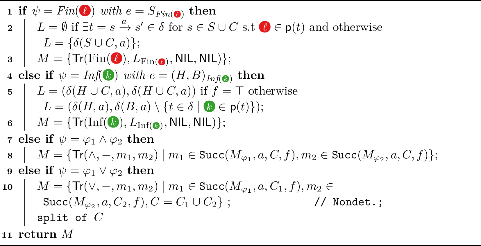
Figure 2: \(\mathtt{Succ}\) computation with the negated condition \(\psi = \textrm{Inf}(\tikz[baseline=-.33em]\pic{acc=3};) \wedge (\textrm{Fin}(\tikz[baseline=-.33em]\pic{acc=1};) \vee \textrm{Inf}(\tikz[baseline=-.33em]\pic{acc=2};))\)..
To construct \(\delta^{\sharp}\) and \(\mathsf{Acc}^{\sharp}\), we first introduce the notions of successors and satisfiability of a given tree-macrostate. We define the successor construction for tree-macrostates (see 1). Let \(\mathcal{M}_\varphi\) be a tree-macrostate for a subtree \(\varphi\) of \(\psi\), \(a \in \Sigma\), \(C \subseteq \mathcal{Q}_d\), and \(f \in \{\bot,\top\}\) a mode flag, where \(\top\) denotes sampling mode. The set of successor tree-macrostates is defined inductively as specified in 1. Observe that, for \(\mathsf{Fin}\)-leaves, the presence of a \(\tikz[baseline=-.33em]\pic{cacc={5}{\upshape \ell}};\)-labelled transition eliminates all successors. Moreover, the flag \(f\) is only relevant for \(\mathsf{Inf}\)-leaves: if \(f = \top\), the breakpoint set \(B\) is resampled; if \(f = \bot\), it continues to track runs that have not visited \(\tikz[baseline=-.33em]\pic{cacc={4}{\upshape k}};\).
Example 1.
Consider the automaton in 2 (a) with negated acceptance condition \(\psi = \textrm{Inf}(\tikz[baseline=-.33em]\pic{acc=3};) \wedge (\textrm{Fin}(\tikz[baseline=-.33em]\pic{acc=1};) \vee \textrm{Inf}(\tikz[baseline=-.33em]\pic{acc=2};))\). Consider the tree-macrostate \(\mathcal{M}_\psi\) in 2 (b), with \(C = \{q\}\) and \(f = \top\). At the \(\wedge\)-node, both \(C\) and \(f\) are forwarded to the two children. For the \(\textrm{Inf}(\tikz[baseline=-.33em]\pic{acc=3};)\)-leaf, we have \(H=\{r\}\) and \(B=\emptyset\). Its successors are trees \(\textsf{Tr}(\textrm{Inf}(\tikz[baseline=-.33em]\pic{acc=3};),(\{r,q\}, \{r,q\})_{\textrm{Inf}(\tikz[baseline=-.33em]\pic{acc=3};)}, \textsf{NIL}, \textsf{NIL})\), since \(\delta(H\cup C, a) = \delta(\{r,q\}, a) = \{r,q\}\) and \(f = \top\) (hence \(B\) is resampled). At the \(\vee\)-node, \(C\) is nondeterministically split into \(C_1 \cup C_2\). If \(C_1=\emptyset\) and \(C_2=\{q\}\), then at the \(\textrm{Fin}(\tikz[baseline=-.33em]\pic{acc=1};)\)-leaf, we have \(\delta(\{r\},a)=\{r\}\), as no state in \(S \cup C_1 = \{r\}\) admits a \(\tikz[baseline=-.33em]\pic{cacc={1}{\upshape 1}};\)-colored transition. The \(\textrm{Inf}(\tikz[baseline=-.33em]\pic{acc=2};)\)-leaf resamples its breakpoint (since \(f=\top\)) and returns trees \(\textsf{Tr}(\textrm{Inf}(\tikz[baseline=-.33em]\pic{acc=3};), (\{q\}, \{q\})_{\textrm{Inf}(\tikz[baseline=-.33em]\pic{acc=3};)}, \textsf{NIL}, \textsf{NIL})\), because \(\delta(H \cup C_2, a) = \delta(\{q\}, a) = \{q\}\).
If \(C_1=\{q\}\) and \(C_2=\emptyset\), then at the \(\textrm{Fin}(\tikz[baseline=-.33em]\pic{acc=1};)\)-leaf it obtains \(S \cup C_1 = \{r,q\}\). Since \(q \xrightarrow{a} q\) is \(\tikz[baseline=-.33em]\pic{cacc={1}{\upshape 1}};\)-colored, it returns \(\emptyset\), and this branch yields no successor.
We say that a tree-macrostate is satisfied if all its \(\mathsf{Inf}\)-leaves have empty breakpoints. Formally, we define \(\mathtt{IsSat}\) inductively over subtrees of \(\psi\) by \(\mathtt{IsSat}(\mathcal{M}_{\varphi_1 \star \varphi_2}) = \mathtt{IsSat}(\mathcal{M}_{\varphi_1}) \wedge \mathtt{IsSat}(\mathcal{M}_{\varphi_2})\) with \(\star \in \{\wedge, \vee\}\), \(\mathtt{IsSat}(M_{\textrm{Fin}(\scalebox{0.6}{\tikz[baseline=-.33em]\pic{cacc={5}{\upshape \ell}};})}) = \top\), and \(\mathtt{IsSat}(M_{\textrm{Inf}(\scalebox{0.6}{\tikz[baseline=-.33em]\pic{cacc={4}{\upshape k}};})}) \iff B = \emptyset\) where \(B\) is the breakpoint set of \(M_{\textrm{Inf}(\scalebox{0.6}{\tikz[baseline=-.33em]\pic{cacc={4}{\upshape k}};})}\).
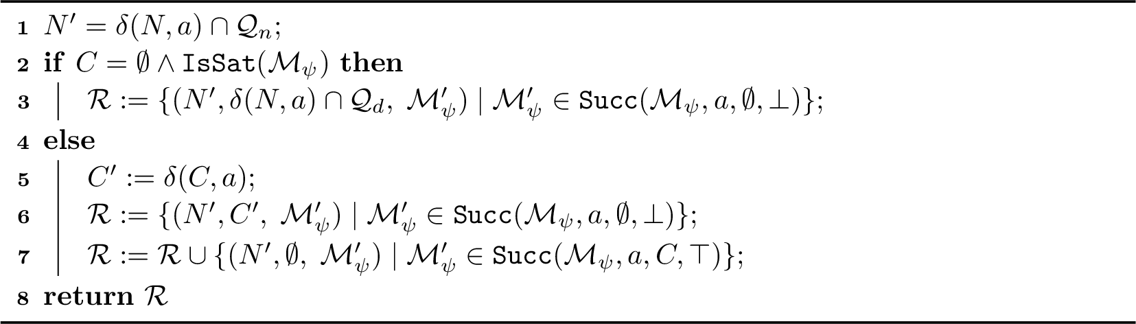
Now we have all the ingredients to construct \(\delta^{\sharp}\) and \(\mathsf{Acc}^{\sharp}\). Intuitively, \(\mathcal{A}^{\sharp}\) operates in two alternating phases that repeat infinitely often: First, in the sampling mode, the construction samples runs entering \(\mathcal{Q}_d\) by maintaining a set \(C\). This mode must repeat infinitely often to ensure that every run is eventually tracked and checked against \(\psi\). Second, in the checking mode, The sampled runs are verified to ensure that all of them satisfy \(\psi\). Formally, \(\delta^{\sharp}\) is defined by Algorithm 3. Its behavior depends on the value of \(C\). When \(C = \emptyset\) and \(\mathtt{IsSat}(\mathcal{M}_\psi)\) (i.e., checking mode has been successfully completed), an accepting mark is emitted and \(C\) is replenished with all states from \(N \cap \mathcal{Q}_d\) to begin a fresh sampling cycle. Otherwise, the automaton is in the checking phase, meaning that some breakpoint set is not yet empty. In this case, we proceed nondeterministically: either the successors are computed without resampling, i.e., \(f=\bot\), thereby continuing the verification of the currently tracked runs (see Line [line:checking]), or we choose to start a new sampling cycle by initiating resampling (see Line [line:sampling]), which nondeterministically assigns all current runs in \(C\) into leaf nodes (see Line [line:sampling]). Finally, the accepting condition of \(\mathcal{A}^{\sharp}\) is \(\mathsf{Acc}^{\sharp}= \{ (N, C, \mathcal{M}_\psi) \xrightarrow{a} (N', C', \mathcal{M}_\psi') \in \delta^{\sharp}\mid C = \emptyset, \mathtt{IsSat}(\mathcal{M}_\psi) \}\). Let \(\psi^{\text{DNF}}\) be the disjunctive normal form of \(\psi\). Then \(\mathsf{Acc}^{\sharp}\) ensures that each run of the input word either never enters the deterministic component or, after entering, satisfies some conjunct of \(\psi^{\text{DNF}}\) by visiting infinitely colours of all \(\mathsf{Inf}\)-leaves while avoiding colours of all \(\mathsf{Fin}\)-leaves. It follows that \(\mathcal{L}(\mathcal{A}^{\sharp})\subseteq \mathcal{L}(\mathcal{A})\). Conversely, for every word not accepted by, there exists a correct nondeterministic choice for runs expected to satisfy a disjunct in \(\psi^{\text{DNF}}\). Along such a macrorun, the breakpoint sets associated with all \(\mathsf{Inf}\)-leaves are cleared infinitely often, while no \(\mathsf{Fin}\)-conditions are violated. Hence, \(\Sigma^\omega\setminus \mathcal{L}(\mathcal{A})\subseteq \mathcal{L}(\mathcal{A}^{\sharp})\).
Therefore, we obtain our main result:
Theorem 5. \(\mathcal{L}(\mathcal{A}^{\sharp})= \Sigma^\omega\setminus \mathcal{L}(\mathcal{A})\).
5.1 Tree-Macrostate Normalization↩︎
Two runs may merge along a word. Consequently, after computing successors over a letter, a successor tree-macrostate may contain redundant run tracking, in particular when the same state appears in multiple subtrees of a \(\vee\)-node and is checked independently. In such cases, we retain only the rightmost occurrence and enforce disjointness among the subtrees of each \(\vee\)-node. Intuitively, once two runs merge, one can be discarded, as its finite prefix does not affect the satisfaction of any acceptance condition. This normalization preserves correctness. We refer to 10.1 for details.
5.2 Shared Breakpoint Optimization↩︎
In the base construction, each \(\textrm{Inf}\)-leaf maintains its own breakpoint, leading to a state-space factor of \(|2^{\mathcal{Q}_d}|^k\) for a subtree with \(k\) \(\mathsf{Inf}\)-leaves. We can apply a standard round-robin technique to track one \(\mathsf{Inf}\)-leaf at a time using a shared breakpoint, reducing the factor to \(k \cdot |2^{\mathcal{Q}_d}|\). Concretely, the construction cycles through the \(\mathsf{Inf}\)-leaves, verifying each leaf in turn before proceeding to the next, and restarting the cycle thereafter. This optimization preserves correctness while avoiding independent breakpoint tracking.
To implement this, we attach a context \(\mathit{ctx} = (h, j, \mathbb{L}, B_{\mathit{sh}})\) to selected nodes, which maintain the shared breakpoint. The phase \(h \in \{\mathit{W}, \mathit{R}, \mathit{P}\}\) indicates whether the cycle is waiting for the next sampling, resampling the shared breakpoint for the current leaf, or processing the current breakpoint. The sequence \(\mathbb{L}= \langle u_1,\dots,u_k \rangle\) orders the \(\mathsf{Inf}\)-leaves, \(j\) denotes the currently tracked leaf, and \(B_{\mathit{sh}} \subseteq \mathcal{Q}_d\) is the shared breakpoint. Individual breakpoints are removed under this optimization. A tree-macrostate may contain multiple such contexts; details are given in 10.2.
5.3 OR-FIN Optimization↩︎
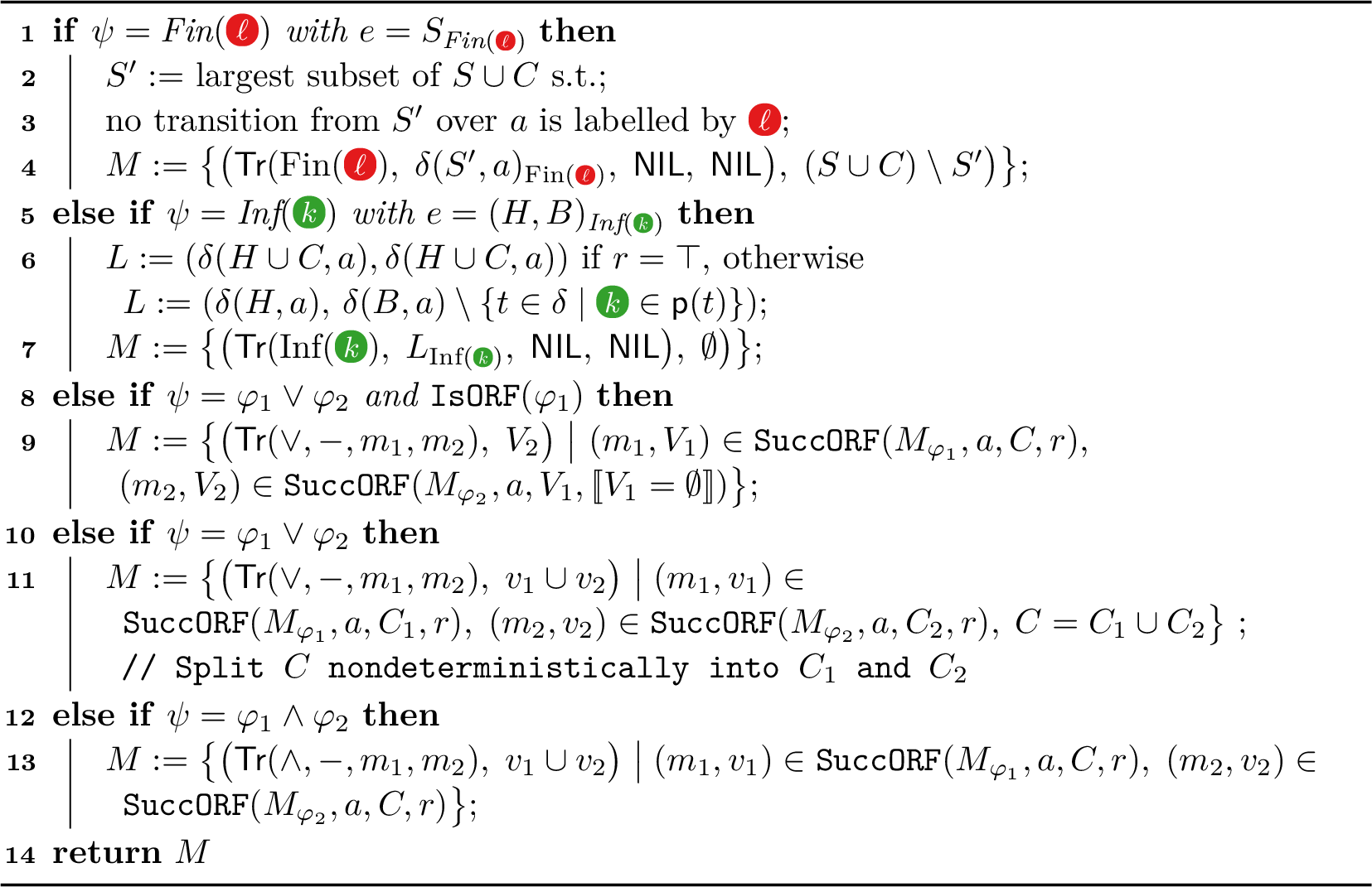
In the base construction, \(\mathtt{Succ}\) for a \(\vee\)-node nondeterministically partitions the states in \(C\) across its children, yielding \(2^{|C|}\) successors. The OR-FIN optimization avoids this blowup when the left child \(\varphi_1\) is an \(\mathtt{IsORF}\) subtree, i.e., a \(\vee\)-composition of \(\textrm{Fin}\)-leaves. The key idea is to propagate violating states sequentially: a \(\textrm{Fin}\)-leaf \(\textrm{Fin}\) filters violating states/runs and passes them to the next \(\textrm{Fin}\)-leaf. These states/runs are eventually either absorbed by an \(\textrm{Inf}\)-leaf or cause rejection if they reach the root. This is correct because a run needs to satisfy at least one branch of the \(\vee\)-subtree; thus, it suffices to check the \(\textrm{Fin}\)-leaves one after another. If a run violates all of them, it is correctly rejected; otherwise, it is accepted as soon as one condition is met. This eliminates the need for exponential branching while preserving correctness. Details of the construction are provided in 10.3.
5.4 Complexity Analysis↩︎
Consider an ELSA \(\mathcal{A}\) with \(n\) states \(\mathcal{Q}= \mathcal{Q}_n \cup \mathcal{Q}_d\) and an Emerson-Lei condition \(\mathsf{Acc}\), together with its complement \(\mathcal{A}^{\sharp}\) constructed by the inductive procedure above. Let \(\psi = \lnot \mathsf{Acc}\) with \(x\) being the number of \(\mathsf{Fin}\) atoms, and \(y\) being the number of \(\mathsf{Inf}\) atoms. We define \(d\) as the maximum number of \(\mathsf{Inf}\)-leaves in a \(\land\)-only subtree of \(\psi\), and \(m\) as the number of \(\land\)-only maximal subtrees of \(\psi\) (i.e., \(\land\)-only subtrees not contained inside larger \(\land\)-only subtrees). Moreover, \(m \leq y\) refers to the number of contexts generated by the shared breakpoint optimization (5.2), and \(d\) is the maximum number of leaves that contexts may schedule. Observe that \(x\), \(y\), \(m\), and \(d\) are upper-bounded by the number of atoms of \(\mathsf{Acc}\).
The states of \(\mathcal{A}^{\sharp}\) hold a set \(N \subseteq \mathcal{Q}_n\), a set \(C \subseteq \mathcal{Q}_d\), and a tree-macrostate \(\mathcal{M}_{\psi}\). Without optimization, \(\mathcal{M}_{\psi}\) holds \(x\) sets \(S \subseteq \mathcal{Q}_d\) (one per \(\mathsf{Fin}\)-leaf), and \(y\) pair of sets \((S, B) \subseteq \mathcal{Q}_d^2\) (one per \(\mathsf{Inf}\)-leaf). With the shared breakpoint optimization, \(\mathcal{M}_{\psi}\) holds \(x+y\) sets \(S \subseteq \mathcal{Q}_d\) (one per leaf), and \(m\) contexts. Each context keeps a phase status \(p \in \{W, R, P\}\), a counter \(i \in \{1, \ldots, d\}\), a set of at most \(d\) identifiers among \(\mathsf{Inf}\)-leaves \(\mathbb{L}\), and a breakpoint \(B_{\mathit{sh}}\subseteq \mathcal{Q}_d\). Note that \(\mathbb{L}\) is fully determined by the formula, and thus it is independent of the size of \(\mathcal{A}^{\sharp}\).
We establish an upper bound on the number of states of \(\mathcal{A}^{\sharp}\) by determining, for each state of \(\mathcal{A}\), the internal subsets of a macrostate in which it may appear. For readability we define, for the considered macrostates, \(S_{\mathsf{Fin}} \subseteq \mathcal{Q}_d^{x}\), \(S_{\mathsf{Inf}} \subseteq \mathcal{Q}_d^{y}\), and \(B_{cxt}\subseteq \mathcal{Q}_d^{m}\) respectively the collection of the sets appearing on \(\mathsf{Fin}\)-leaves, \(\mathsf{Inf}\)-leaves, and shared breakpoint of contexts. Given a state \(q\) of \(\mathcal{A}\), the possibilities are that \(q\) may be in no subsets or
\(q\) belongs nowhere,
\(q\) belongs in \(C\) or not,
\(q\) belongs in \(S_{\mathsf{Inf}}\),
\(q\) belongs in both \(S_{\mathsf{Inf}}\) and \(B_{cxt}\), and
\(q\) belongs in some \(S_{\mathsf{Fin}}\).
We have thus \((1+ 2 \times 2^{y} \times 2^{x} \times 2^{m})^{n}\) cases. Including the data carried by each context, namely, the phase and the counter, generate copies. We get that the state-space of \(\mathcal{A}^{\sharp}\) is bounded by \(3 \max\{d,1\} (1 + 2 \times 2^{y} \times 2^{x} \times 2^{m})^{n}\). We can further reduce this bound when a certain property holds. Concretely, when sets appearing in \(\mathsf{Fin}\)-leaves are disjoint, which is caused when all \(\mathsf{Fin}\)-leaves are in a subtree without \(\land\)-nodes, we get \(3 \max\{d,1\} (1 + 2 \times 2^{y} \times (x+1) \times 2^{m})^{n}\). When additionally the whole negated acceptance condition \(\psi\) has no conjunction (e.g., \(\mathsf{Acc}\) is a generalized Rabin pair), we have the property that sets of all tree-macrostate leaves are disjoint (the breakpoint set is still a subset of a particular \(\textrm{Inf}\)-leaf), so we get \(3 \max\{d,1\}(1 + 2 \times 2^{y} \times (x + m + 1))^{n}\). Upper bounds for popular acceptance conditions are given in 1 with a more detailed analysis given in 11. We note that we could obtain better bounds for the concrete constructions in [sec:rabin] [sec:streett] because of more fine-tuned construction and analysis.
6 Complementation of an ELEA and a General ELA↩︎
Modular construction of an ELEA.
To lift the complementation procedure from semi-deterministic to elevator automata, we employ the modular complementation approach [21] generalized to the ELA setting. The modular construction decomposes complementation of the whole automaton \(\mathcal{A}\) into complementation algorithms for individual SCCs or groups of SCCs called partitions. Each partial complementation algorithm specifies its own macrostates, transition function, coloring, and acceptance condition. The transition function takes into account runs entering the partition from outside. The inductive construction from 5 fits naturally into this framework: the macrostates of the partial algorithm take the form \((C,\mathcal{M}_\psi)\), where the \(N\) component is omitted since incoming runs are tracked by the top-level modular algorithm. Concretely, in 3 the set \(N'\) represents the newly incoming runs supplied by the top-level algorithm, and \(\mathcal{Q}_d\) denotes the states of the deterministic partition. To obtain a complete complementation algorithm for ELEAs, we additionally plug the Miyano-Hayashi algorithm [27] into the modular construction to handle inherently-weak partitions and the same algorithm with round robin (similar to the procedure in 4) to handle generalized co-Büchi partitions with the complexity \(\mathcal{O}(3^n)\) and \(\mathcal{O}(k\cdot(3^n))\) respectively. An example of the modular construction is shown in 12.
Elevatorization of ELAs.
Any ELA can be transformed into an equivalent ELEA, which lifts our techniques to the general case. The conversion treats each SCC independently. In particular, nondeterministic accepting components (NACs) must be semi-determinized [11] since they violate the elevator condition. Because semi-determinization yields only inherently-weak and deterministic components, the resulting automaton is an ELEA. Let \(\mathcal{A}\) be an ELA with acceptance condition \(\mathsf{Acc}\). For each NAC, \(\mathsf{Acc}\) can be simplified to contain only colors appearing in the NAC. This yields a smaller local condition that is used in place of \(\mathsf{Acc}\) when applying the semi-determinization construction of [29] to the corresponding NAC. After semi-determinization, a copy of the NAC without colors is connected to a deterministic part that emits a fresh color \(\tikz[baseline=-.33em]\pic{cacc={4}{\upshape \top}};\), and \(\mathsf{Inf}(\tikz[baseline=-.33em]\pic{cacc={4}{\upshape \top}};)\) becomes the acceptance condition of this semi-deterministic component. To prevent interference between SCCs of \(\mathcal{A}\), we disable \(\mathsf{Acc}\) within all semi-determinized components by marking them with a fresh color \(\tikz[baseline=-.33em]\pic{cacc={5}{\upshape \bot}};\), and adopt \((\mathsf{Acc}\land \mathsf{Fin}(\tikz[baseline=-.33em]\pic{cacc={5}{\upshape \bot}};)) \lor \mathsf{Inf}(\tikz[baseline=-.33em]\pic{cacc={4}{\upshape \top}};)\) as the global acceptance condition. The semi-determinization of [29] runs in \(\mathcal{O}(2^{|\varphi|+|Q|})\), where \(Q\) is the set of states and \(\varphi\) is the simplified acceptance condition of the given SCC. Details are given in 13.
7 Experimental Evaluation↩︎
Implementation.
We extended Kofola [12] with direct support for ELA complementation and integrated the inductive construction into its modular framework. We evaluate four configurations of the inductive construction:
Kofola-Ind: the base inductive construction without any optimizations;
Kofola-Ind-SHB-Root: includes the shared breakpoint optimization, where a single context is maintained at the root of each tree-macrostate;
Kofola-Ind-SHB-Subtree: includes the shared breakpoint optimization, where a context is maintained within each subtree consisting solely of \(\land\)-nodes and \(\textrm{Inf}\)-leaves (allowing multiple contexts per tree-macrostate); and
Kofola-Ind-FOR: employs the OR-FIN optimization.
Used tools and environment.
We experimentally evaluated the inductive construction and compared it with the state-of-the-art tool Spot [25] (we use a custom build with the maximum number of colors increased from 32 to 128) and its variant Spot-High, which applied Spot’s High reduction on the output. All experiments were conducted on an Ubuntu GNU/Linux 24.04 virtual machine with 64 GiB of RAM, running on an AMD EPYC 9124 CPU server under the Proxmox Virtual Environment. The timeout was 120 s. The
correctness of results was validated by cross-checking the outputs using Spot’s autcross.
Benchmarks.
Our evaluation is based on the following three data sets (available at [30]):
Existing LTL benchmarks. We used a collection of LTL formulas from the literature, taken from the benchmarks used in the evaluation of
ltl3tela[26]. The benchmark set is available in theltl3telarepository [31] and is based on formulas generated bygenltlas well as formulas collected from prior work. After filtering out trivial cases, this resulted in 1,378 instances. These automata were then transformed into elevator automata. We denote this benchmark as LTL-Lit.Randomly generated automata. We generated 315 automata with a single generalized Rabin pair acceptance and transformed them into elevator automata while preserving the generalized Rabin pair acceptance form. We denote this benchmark as GRA.
Random LTL formulas. We used Spot’s
randltlwith parameters-l --seed=42128971 --weak-fairness -n -1 --simplify=0 a b c d eto generate random LTL formulas. The generated formulas were subsequently translated into automata in theHOAformat usingltl3tela[26]. We usedautfiltto remove trivial automata (such as deterministic, weak, empty, or terminal ones), and kept only elevator automata. This way, we obtained 1,000 instances. We denote this benchmark as LTL-Rand.
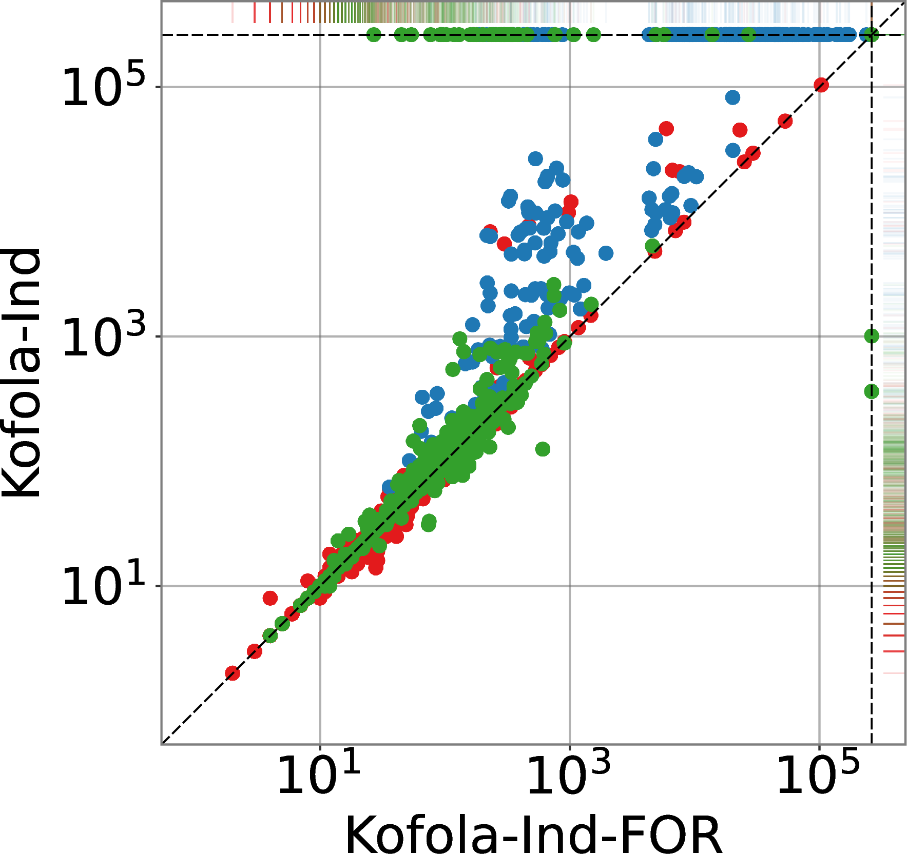
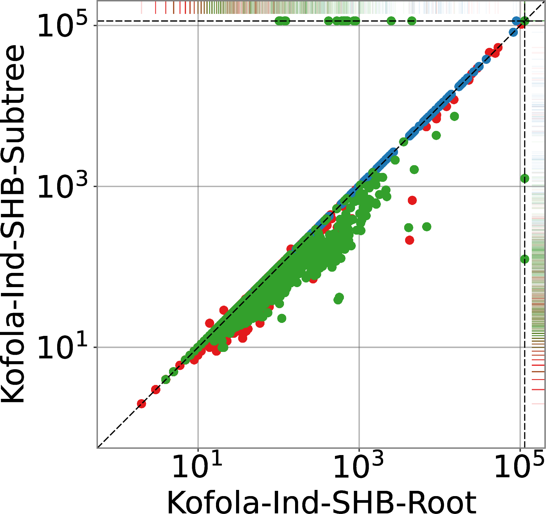
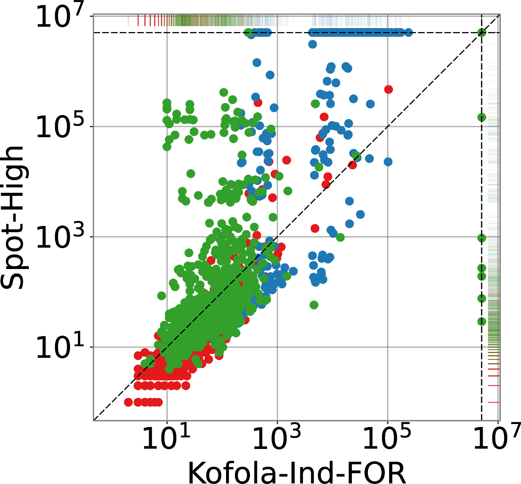
Figure 4: Scatter-plots comparing sizes of complemented automata (in the number of states). Colors denote benchmarks: \(\bullet\) GRA, \(\bullet\) LTL-Rand, and \(\bullet\) LTL-Lit.. a — sec:, b — sec:, c — sec:
| tool | unsolved | average | median | total states | time | |
|---|---|---|---|---|---|---|
| 40 | 2,436 | 25 | 6,463,028 | 2,828 | ||
| 247 | 537 | 21 | 1,312,689 | 3,629 | ||
| 226 | 639 | 26 | 1,576,427 | 3,502 | ||
| 242 | 547 | 23 | 1,339,994 | 3,066 | ||
| 156 | 15,058 | 39 | 38,202,295 | 673 | ||
| 159 | 11,136 | 15 | 28,218,675 | 1,167 |
Discussion.
We give the results comparing sizes of outputs of our four configurations and Spot in 4 2. 4 (a) evaluates the OR-FIN optimization (5.3) against the baseline; it shows that the optimization is mostly advantageous and essential for solving some benchmarks (it solves 207 more benchmarks than the baseline; we note that in a few cases, the baseline, however, could solve some benchmarks that the optimization could not). The second plot, in 4 (b), evaluates the two shared breakpoint optimizations; it shows that although Kofola-Ind-SHB-Root solves slightly more benchmarks, Kofola-Ind-SHB-Subtree almost always outputs a slightly smaller automaton (if it finishes). The last plot, 4 (c), evaluates our best configuration, Kofola-Ind-FOR, against Spot-High; on a part of the inputs, the two tools give comparable results (Spot-High in many cases giving slightly smaller outputs), however, on more challenging inputs, Kofola-Ind-FOR mostly dominates Spot-High by a large margin and can solve 119 more benchmarks.
In 2, we provide statistical data for our experiments. We highlight Kofola-Ind-FOR, which solved the most benchmarks by a large margin (the second one was Spot with 116 less solved benchmarks). Although the average size of the output is larger than other configurations of Kofola, this is mostly because Kofola-Ind-FOR can complement many of the more challenging inputs (this also holds for the median and the total number of states). On the other hand, even with the more finished runs, Kofola-Ind-FOR was the fastest configuration of Kofola(but still not as good as Spot—which is quite optimized—when we compare the runtime on only finished instances). The emphasize the total number of states generated by Kofola-Ind-FOR: roughly \(4.4\times\) less than Spot-High despite solving many more cases.
8 Related Work↩︎
Complementation of finite automata on infinite words is a problem addressed since the trailblazing work of Büchi [8]. For the basic model of Büchi automata, the lower bound for the problem is \(\Omega((0.76n)^n)\) established using the full automata technique in [32] by Yan (improving the previous \(\Omega(n!)\) lower bound of Michel [33]). A multitude of approaches for complementing BAs have been proposed in the literature, e.g., Ramsey-based [8], [34], [35], rank-based [10], [20], [36]–[40], determinization-based [41]–[43], slice-based [44], and others [21], [45], [46]. Some of these approaches [20], [45] even match the lower bound (modulo a small polynomial factor). More efficient complementation algorithms for structural subclasses of BAs were also considered, e.g., for inherently-weak (\(\frac{2}{3} 3^n\)) [27], deterministic (\(n+1\) with output being a co-Büchi automaton or \(2n\) with output being a BA) [47], semideterministic (\(4^n\)) [28], [48], elevator (a GBA with \(4^n\) states and two colors) [10], [21], or unambiguous (\(4^n\)) [49], [50] BAs.
The landscape is considerably less explored for richer acceptance conditions (we recommend Boker’s excellent survey [13] and its accompanying web page for more details and references). For generalized BAs (GBAs) with \(n\) states and \(k\) acceptance sets, [51] gives a complementation algorithm with the complexity \(2^{\mathcal{O}(n \log kn)}\). The GBA complementation algorithm given in [19] produces a result as a BA with \(\mathcal{O}(n(0.76nk)^n)\) states and [52] claims to improve over this. Co-Büchi automata can be complemented into BAs with \(\frac{2}{3} 3^n\) states [13], [27]. For a Rabin automaton with \(n\) states and \(\ell\) pairs, the algorithm in [53] produces a complement BA with \(\mathcal{O}(\ell \cdot 3^n \cdot (2n+1)^{n\ell})\) states and the one in [19] produces a GBA with \(\mathcal{O}(n^\ell(0.76n)^{n\ell})\) states and \(\ell\) colours. Streett automata can be complemented into BAs with \(2^{\mathcal{O}(n\ell \log n \ell)}\) states using [53] and into BAs with \(2^{\mathcal{O}(n \log n + n\ell \log \ell)}\) states [24]. Parity automata can be complemented into BAs with \(2^{\mathcal{O}(n \log n)}\) states. In [15], it is shown that the lower bound for the number of states of a complement of an ELA is \(2^{2^n}\) (even if the output can also be an ELA), and the same work shows that the upper bound is \(2^{2^{\mathcal{O}(n)}}\) (not considering the complexity of the acceptance condition as a parameter). This was refined in [19], which gave an algorithm that produces a GBA with \(2^k\) colors and \(\mathcal{O}(n^{2^k}(0.76nk)^{n2^k})\) states, where \(n\) is the number of states of the input ELA and \(k\) is the number of colors that occur in the acceptance condition. All of our upper bounds are better.
Elevator automata were introduced in [10] in the context of rank-based complementation as a subclass of BAs with a more efficient complementation procedure (\(\mathcal{O}(16^n)\)). Since then, it was shown that there exists on optimal determinization procedure (\(\mathcal{O}(n!)\)) [43] and an efficient complementation procedure (\(\mathcal{O}(4^n)\)) [21] for them. A recent paper [12] shows that the vast majority of BAs considered in practical scenarios are elevator automata.
9 Proof of 4↩︎
We can deduce the bound on the number of states of \(\mathcal{A}^{\sharp}\) by checking, for each state \(q \in \mathcal{Q}\), in which internal sets of a macrostate \(\mathcal{M}= (N,\mathit{CR}, S, B, z)\) it can be and give each such a choice a number \(f(q)\) as follows:
If \(q\) is not present in \(\mathcal{M}\) at all, we assign \(f(q) = 1\).
We do a case split on the value of \(z\). For \(z=0\) (tracking \(\mathsf{Inf}(\tikz[baseline=-.33em]\pic{acc=0};)\)):
If \(q \in \mathcal{Q}_n \cap N\) or \(q \in \mathcal{Q}_d \cap \mathit{CR}\cap B\), we assign \(f(q) = 2\) (i.e., we can merge \(N\) and \(\mathit{CR}\cap B\) similarly as for a generalized Rabin pair).
If \(q \in (\mathit{CR}\cap S)\), we let \(f(q) = 3\) and if \(q \in \mathit{CR}\setminus (S \cup B)\), we let \(f(q) = 4\). We note that the case \(\mathit{CR}\cap S \cap B\) does not need to be considered since for \(z=0\), the sets \(S\) and \(B\) are disjoint.
For \(z >0\) (tracking \(\mathsf{Fin}(\tikz[baseline=-.33em]\pic{cacc={2}{\upshape j}};)\)):
If \(q \in \mathcal{Q}_n \cap N\) or \(q \in \mathcal{Q}_d \cap \mathit{CR}\cap B \cap S\), we assign \(f(q) = 2\).
If \(q \in (\mathit{CR}\cap S) \setminus B\), we let \(f(q) = 3\) and if \(q \in \mathit{CR}\setminus S\), we let \(f(q) = 4\). We note that the case \(\mathit{CR}\cap (B \setminus S)\) does not need to be considered since for \(z>0\) we have \(B \subseteq S\).
The total number of functions \(f\colon \mathcal{Q}\to \{1, \ldots, 4\}\) is \(4^n\) where \(n = |\mathcal{Q}|\). Since \(z\) is between \(0\) and \(k\), we obtain \((k+1)\cdot 4^n\).
10 Detailed Optimizations↩︎
10.1 Tree-macrostate Reduction↩︎
After computing the successor of a tree-macrostate, the resulting tree may contain runs that are checked by multiple leaves. In particular, the same state may appear in both branches of a \(\vee\)-node and thus be checked independently along each branch, although it suffices to check it on one branch only. The tree-macrostate reduction eliminates this redundancy by enforcing disjointness at \(\vee\)-nodes without affecting correctness.
Tree-macrostate restriction.
We first define a \(\mathtt{gather}(\mathcal{M}_\varphi)\) function that collects all states referenced by a tree-macrostate: \[\begin{align} \mathtt{gather}(\mathcal{M}_{\varphi_1 \wedge \varphi_2}) &= \mathtt{gather}(\mathcal{M}_{\varphi_1}) \cup \mathtt{gather}(\mathcal{M}_{\varphi_2}) && \mathtt{gather}(S_{\textrm{Fin}(\scalebox{0.6}{\tikz[baseline=-.33em]\pic{cacc={5}{\upshape \ell}};})}) = S \\ \mathtt{gather}(\mathcal{M}_{\varphi_1 \vee \varphi_2}) &= \mathtt{gather}(\mathcal{M}_{\varphi_1}) \cup \mathtt{gather}(\mathcal{M}_{\varphi_2}) && \mathtt{gather}((H,B)_{\textrm{Inf}(\scalebox{0.6}{\tikz[baseline=-.33em]\pic{cacc={4}{\upshape k}};})}) = H \end{align}\] Note that only the track set is gathered from \(\textrm{Inf}\)-leaves; the breakpoint \(B\) is not considered, as it is a subset of the track set. Further, for a set of states \(R\subseteq \mathcal{Q}_d\) we define the tree-macrostate restriction \(\mathcal{M}_\varphi{|}_{F}\) for removing \(R\) from every leaf in the tree: \[\begin{align} \mathcal{M}_{\varphi_1 \wedge \varphi_2}{|}_{R} &= \mathcal{M}_{\varphi_1}{|}_{R} \wedge \mathcal{M}_{\varphi_2}{|}_{R} && S_{\textrm{Fin}(\scalebox{0.6}{\tikz[baseline=-.33em]\pic{cacc={5}{\upshape \ell}};})}{|}_{R} = (S \setminus R)_{\textrm{Fin}(\scalebox{0.6}{\tikz[baseline=-.33em]\pic{cacc={5}{\upshape \ell}};})} \\ \mathcal{M}_{\varphi_1 \vee \varphi_2}{|}_{R} &= \mathcal{M}_{\varphi_1}{|}_{R} \vee \mathcal{M}_{\varphi_2}{|}_{R} && (H,B)_{\textrm{Inf}(\scalebox{0.6}{\tikz[baseline=-.33em]\pic{cacc={4}{\upshape k}};})}{|}_{R} = (H \setminus R,\; B \setminus R)_{\textrm{Inf}(\scalebox{0.6}{\tikz[baseline=-.33em]\pic{cacc={4}{\upshape k}};})} \end{align}\] For \(\textrm{Inf}\)-leaves, both the track set and the breakpoint are restricted, since the breakpoint is always a subset of the track set and must remain consistent with it.
Reduction.
The reduction \(\mathtt{clip}(\mathcal{M}_\varphi)\) is defined recursively over the tree-macrostate structure: \[\begin{align} \mathtt{clip}(\mathcal{M}_{\varphi_1 \wedge \varphi_2}) &= \mathtt{clip}(\mathcal{M}_{\varphi_1}) \wedge \mathtt{clip}(\mathcal{M}_{\varphi_2}) && \mathtt{clip}(S_{\textrm{Fin}(\scalebox{0.6}{\tikz[baseline=-.33em]\pic{cacc={5}{\upshape \ell}};})}) = S_{\textrm{Fin}(\scalebox{0.6}{\tikz[baseline=-.33em]\pic{cacc={5}{\upshape \ell}};})} \\ \mathtt{clip}(\mathcal{M}_{\varphi_1 \vee \varphi_2}) &= \mathtt{clip}\!\left(\mathcal{M}_{\varphi_1}{|}_{\mathtt{gather}(\mathcal{M}_{\varphi_2}')}\right) \vee \mathcal{M}_{\varphi_2}' && \mathtt{clip}((H,B)_{\textrm{Inf}(\scalebox{0.6}{\tikz[baseline=-.33em]\pic{cacc={4}{\upshape k}};})}) = (H,B)_{\textrm{Inf}(\scalebox{0.6}{\tikz[baseline=-.33em]\pic{cacc={4}{\upshape k}};})} \end{align}\] where \(\mathcal{M}_{\varphi_2}' = \mathtt{clip}(\mathcal{M}_{\varphi_2})\). Leaf nodes are returned unchanged. For \(\wedge\)-nodes, both children are reduced independently. For a \(\vee\)-node, the right child is reduced first; its states \(\mathtt{gather}(\mathtt{clip}(\mathcal{M}_{\varphi_2}))\) are then removed from the left child before it to be reduced. This ensures that every state appears in at most one branch of each \(\vee\)-node.
10.2 Shared Breakpoint Optimization↩︎
In order to reference a leaf node, we identify leaves with unique identifiers and we refer them as \(\textrm{Inf}_{u}(\tikz[baseline=-.33em]\pic{cacc={4}{\upshape k}};)\)-nodes (\(\textrm{Inf}\)-node identified by \(u\)). The context is assigned to \(\land\)-nodes that are roots of subtrees containing \(\textrm{Inf}\)-leaves (we call such nodes owners of a context). Initially, an owner’s context is \((\mathit{W}, 1, \langle u_1,\dots,u_k\rangle, \emptyset)\) where \(u_1,\dots,u_k\) are the identifiers of all \(\textrm{Inf}\)-leaves in its subtree. When \(\mathtt{Succ}\) is called on an owner, the context is first advanced by \(\mathtt{SuccCtx}\) using the resample flag \(r\), and the updated context is then propagated into the subtree. The procedure \(\mathtt{SuccCtx}\) is given in 5.

Tree successor.
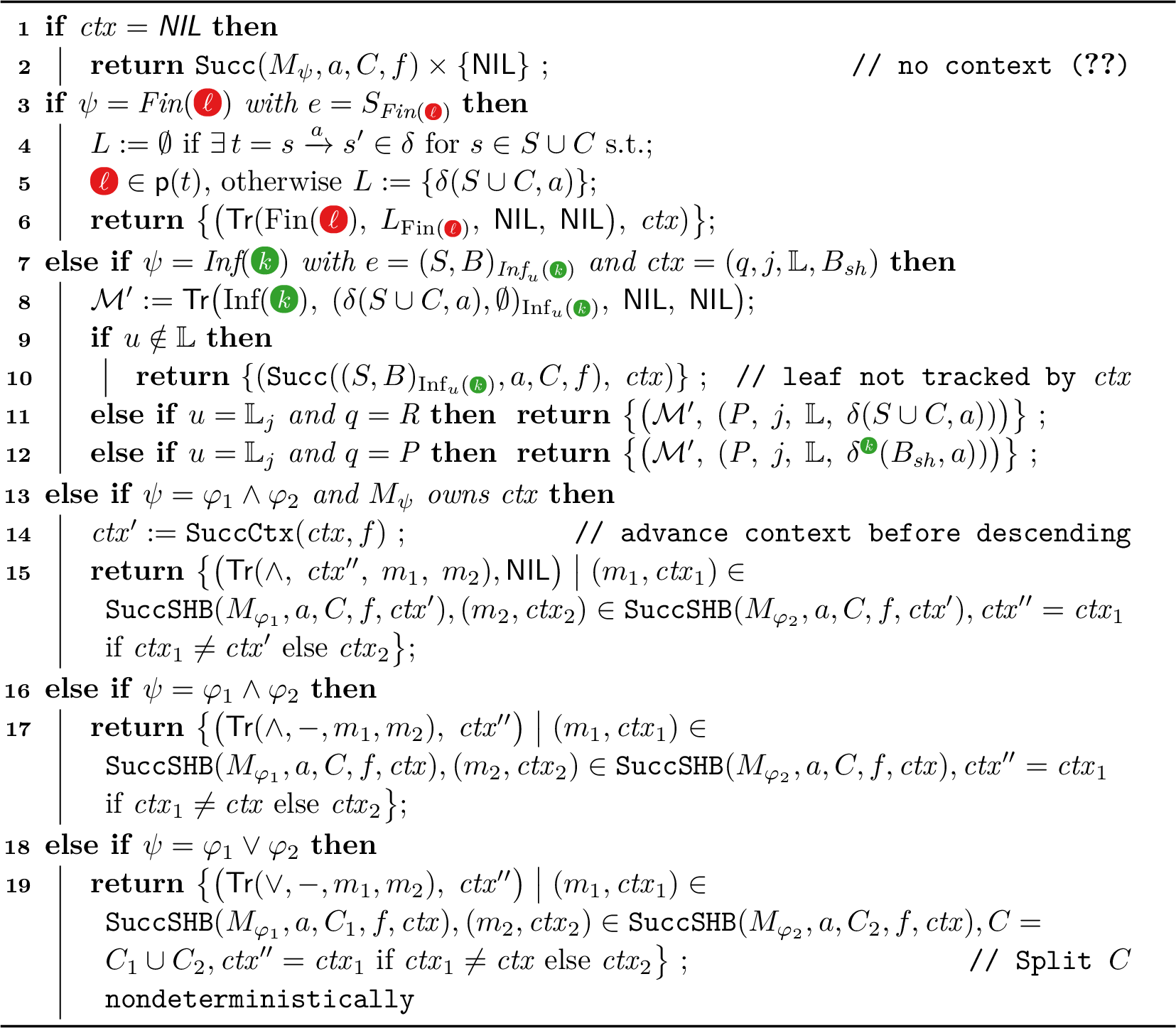
The function \(\mathtt{SuccSHB}(M_\psi, a, C, f, \mathit{ctx})\) extends the base \(\mathtt{Succ}\) with a context parameter \(\mathit{ctx}\) and returns pairs \((m, \mathit{ctx}')\) of a successor tree-macrostate and an updated context. When \(\mathit{ctx} = \textsf{NIL}\), the function immediately falls back to the base inductive successor \(\mathtt{Succ}(M_\psi, a, C, f)\) (cf.1) and returns \(\textsf{NIL}\) as the context. For \(\mathsf{Fin}\)-leaves the successor is computed as in the base construction and the context is passed through unchanged. For an \(\mathsf{Inf}\)-leaf identified by \(u\) with context \((q, j, \mathbb{L}, B_{\mathit{sh}})\), there are three cases: (i) if \(u \notin \mathbb{L}\), the leaf is not tracked by this context and the base successor is used with the context unchanged; (ii) if \(u = \mathbb{L}_j\) and \(q = \mathit{R}\), the leaf resamples the shared breakpoint to \(\delta(S \cup C, a)\) and transitions to phase \(\mathit{P}\); (iii) if \(u = \mathbb{L}_j\) and \(q = \mathit{P}\), the leaf advances the shared breakpoint by removing \(\tikz[baseline=-.33em]\pic{cacc={4}{\upshape k}};\)-coloured transitions. Note that tracked \(\mathsf{Inf}\)-leaves hold \((S, \emptyset)\) — their individual breakpoint is replaced by the shared one — while untracked \(\mathsf{Inf}\)-leaves still carry their own \((S, B)\). For \(\wedge\)-nodes that own the context, the context is first advanced by \(\mathtt{SuccCtx}(ctx, f)\) before descending; the owner stores the updated context returned by whichever child changed it (at most one child modifies the context per step). For all other internal nodes (\(\wedge\) non-owner and \(\vee\)), the context is forwarded to both children and the updated context is selected by the same preference rule. The complete procedure is given in 6.
Satisfaction.
Since Inf-leaves carry no individual breakpoints, a \(\wedge\)-node owning a context \(\mathit{ctx} = (q,j,\mathbb{L},B_{\mathit{sh}})\) is satisfied exactly when the shared cycle has completed, i.e., the context has returned to wait with an empty breakpoint: \[\mathtt{IsSat}\bigl(\mathcal{M}_{\varphi_1 \wedge \varphi_2},\, \mathit{ctx}\bigr) = (q = \mathit{W}\wedge B_{\mathit{sh}} = \emptyset) \wedge\mathtt{IsSat}(\mathcal{M}_{\varphi_1})\wedge \mathtt{IsSat}(\mathcal{M}_{\varphi_2}).\] For the rest of the nodes, the satisfiability remains the same. Using the shared breakpoint optimization we are able to reduce the factor from \(|2^Q|^k\) to \(k|2^Q|\).
10.3 OR-FIN Optimization↩︎
The complete procedure for computing OR-FIN tree-macrostate successor is given in 7. The procedure for computing the transition function \(\delta^{\sharp}\) is given as in 3 with a difference that if \(\mathtt{SuccORF}\) returns nonempty violating states, this tree-macrostate is removed from the set.
11 Detailed Complexity Analysis↩︎
We recall from 5.4 that the size of the complement constructed by our inductive procedure with the shared breakpoint optimization is, in the general case, () \(3 \max\{d,1\}\,(1 + 2 \times 2^{y} \times 2^{x} \times 2^{m})^{n}\). When sets appearing on \(\mathsf{Fin}\)-leaves are disjoint, we have (\(\dagger\)) \(3 \max\{d,1\} (1 + 2 \times 2^{y} \times (x + 1) \times 2^{m})^{n}\). When additionally the negated acceptance condition has no conjunction, we have (\(\ddagger\)) \(3 \max\{d,1\}(1 + 2 \times 2^{y} \times (x + m + 1))^{n}\). 3 provides the detailed upper bounds, where () is used for Rabin, generalized Rabin, and Parity; (\(\dagger\)) is used for generalized co-Büchi, Streett pair, generalized Streett pair, Streett, and generalized Streett; and (\(\ddagger\)) is used for Büchi, generalized Büchi, co-Büchi, Rabin pair, and generalized Rabin pair. For an Emerson–Lei acceptance condition with \(\ell\) leaves, we use () to get \(3\ell \bigl(1 + 2 \times 2^{\ell} \times (2^{\ell} + 2^{\ell})\bigr)^{n} \leq 3\ell \cdot 2^{2\ell+3}\), since \(x\), \(y\), \(d\), and \(m\) are at most \(\ell\).
| Name | Classic | Generalized |
|---|---|---|
| \(\accinfof{\tacc 0}\) | \(\bigwedge_{j=0}^{k-1} \accinfof{\taccj}\) | |
| \(x=1\), \(y=0\), \(d=0\), \(m=0\) | \(x=k\), \(y=0\), \(d=0\), \(m=0\) | |
| \(3 \cdot 5^n\) | \(3 \cdot (2k + 3)^n\) | |
| co- | \(\accfinof{\tacc 0}\) | \(\bigvee_{j=0}^{k-1} \accfinof{\taccj}\) |
| \(x=0\), \(y=1\), \(d=1\), \(m=1\) | \(x=0\), \(y=k\), \(d=k\), \(m=1\) | |
| \(3 \cdot 9^n\) | \(3 \cdot 2^{(k+3)n}\) | |
| Rabin pair | \(\accfinof{B} \land \accinfof{G}\) | \(\accfinof{B} \land \bigwedge_{i=0}^{\ell -1}\accinfof{G_i}\) |
| \(x=1\), \(y=1\), \(d=1\), \(m=1\) | \(x=\ell\), \(y=1\), \(d=1\), \(m=\ell\) | |
| \(3 \cdot 13^{n}\) | \(3 \cdot (8\ell + 5)^{n}\) | |
| Rabin | \(\bigvee_{j=0}^{k-1} \accfinof{B_j} \land \accinfof{G_j}\) | \(\bigvee_{j=0}^{k-1} (\accfinof{B_j} \land \bigwedge_{i=0}^{\ell -1}\accinfof{G_{j,i}})\) |
| \(x=k\), \(y=k\), \(d=1\), \(m=k\) | \(x=k\ell\), \(y=k\), \(d=1\), \(m=k\) | |
| \(3 \cdot 2^{(3k+2)n}\) | \(3 \cdot 2^{(3k\ell+2)n}\) | |
| Streett pair | \(\accinfof{G} \lor \accfinof{B}\) | \(\accinfof{G} \lor \bigvee_{i=0}^{\ell -1}\accfinof{B_i}\) |
| \(x=1\), \(y=1\), \(d=1\), \(m=1\) | \(x=1\), \(y=\ell\), \(d=\ell\), \(m=1\) | |
| \(3 \cdot 17^{n}\) | \(3 \cdot 2^{(\ell+4)n}\) | |
| Streett | \(\bigwedge_{j=0}^{k-1} \accinfof{G_j}\lor \accfinof{B_j}\) | \(\bigwedge_{j=0}^{k-1} (\accinfof{G_j} \lor \bigvee_{i=0}^{\ell-1}\accfinof{B_{j,i}})\) |
| \(x=k\), \(y=k\), \(d=1\), \(m=k\) | \(x=k\), \(y=k\ell\), \(d=\ell\), \(m=k\) | |
| \(6 \cdot k^{n} \cdot 2^{(2k+2)n}\) | \(6 \cdot k^{n} \cdot 2^{(2k\ell+2)n}\) | |
| Parity | \(\accfinof{\tacc 0} \land (\accinfof{\tacc 1} \lor (\accfinof{\tacc 2} \land (\accinfof{\tacc 3} \lor (\accfinof{\tacc 4} \land \ldots \accinfof{\taccgof{k}}) \ldots ))))\) | |
| \((\accfinof{\taccgof{0}} \land \accinfof{\taccgof{1}}) \lor (\accfinof{\taccgof{0,2}} \land \accinfof{\taccgof{1,3}}) \lor \ldots \lor (\accfinof{\taccgof{0, \ldots, k-1}} \land \accinfof{\taccgof{1, \ldots, k}})\) | ||
| \(x=\frac{k}{2}\), \(y=\frac{k}{2}\), \(d=1\), \(m=\frac{k}{2}\) | ||
| \(3 \cdot 2^{(\frac{3}{2}k+2)n}\) | ||
12 Example of the Modular Construction↩︎
An example of the modular construction combining the procedure for the inherently-weak partition and the inductive construction for the deterministic partition is shown in 8.
None
Figure 8: Complementation of the input automaton (left), whose accepting condition is \(\textrm{Fin}(\tikz[baseline=-.33em]\pic{acc=1};) \vee \textrm{Inf}(\tikz[baseline=-.33em]\pic{acc=2};)\), via the modular construction. The resulting automaton (right) has accepting condition \(\textrm{Inf}(\tikz[baseline=-.33em]\pic{acc=0};) \lor (\textrm{Inf}(\tikz[baseline=-.33em]\pic{acc=1};) \land \textrm{Inf}(\tikz[baseline=-.33em]\pic{acc=2};))\)..
13 Elevatorization of ELAs↩︎
Given an ELA \(\mathcal{A}\), we detail here how to construct an equivalent elevator ELA \(\mathcal{A}'\). The procedure first identify the SCCs that violate the elevator property, and then apply an independent semi-determinization algorithm for each of them. Since semi-determinization produces inherently weak and deterministic components, the resulting automaton will be an elevator ELA. Let \(\mathcal{A}= (\mathcal{Q}, \delta, I, \Gamma, \mathsf{p}, \mathsf{Acc})\), and let \(C_1,\ldots,C_{\ell}\) such that \(C_i \subseteq \mathcal{Q}\) be the nondeterministic accepting components (NACs) of \(\mathcal{A}\). For all \(i\), we define \(\Gamma_i\) as the set of colours appearing on the transitions of \(C_i\).
Let \(\mathsf{Acc}^{\text{DNF}} = (\psi_1 \land \varphi_1) \lor \cdots \lor (\psi_{m} \land \varphi_{m})\) be the disjunctive normal form of \(\mathsf{Acc}\) where, for all \(j\), \(\psi_j\) contains only \(\mathsf{Inf}\) predicates and \(\varphi_j\) contains only \(\mathsf{Fin}\) predicates. For each \(i\), we define \(\mathsf{Acc}^{\text{DNF}}_i\) as the simplification of \(\mathsf{Acc}^{\text{DNF}}\) for the component \(C_i\) such that, for all \(c \notin \Gamma_i\), \(\mathsf{Fin}(c)\) is true and \(\mathsf{Inf}(c)\) is false. We get \[\mathsf{Acc}^{\text{DNF}}_i = (\psi_{i, 1} \land \varphi_{i, 1}) \lor \cdots \lor (\psi_{i, m_i} \land \varphi_{i, m_i})\] where \(\psi_{i, j}\) is of the form \(\bigwedge_{k=1}^{n_{i, j}} \mathsf{Inf}(c_{i, j, k})\) and \(\varphi_{i, j}\) is of the form \(\bigwedge_{k=1}^{r_{i, j}} \mathsf{Fin}(d_{i, j, k})\). Let \(\Gamma_{i, j}^{\psi} \subseteq \Gamma_i\) and \(\Gamma_{i, j}^{\varphi} \subseteq \Gamma_i\) be respectively the set of colours appearing in \(\psi_{i, j}\) and \(\varphi_{i, j}\).
The elevator automaton \(\mathcal{A}' = (\mathcal{Q}', \delta', I', \Gamma', \mathsf{p}', \mathsf{Acc}')\) is defined as follows.
We have \(\mathcal{Q}' = \mathcal{Q}\cup \bigcup_{i=1}^{\ell} \bigcup_{j=1}^{m_i} D_{i,j}\) where, for each \(C_i\) and each disjunct \((\psi_{i,j} \land \varphi_{i, j})\) of \(\mathsf{Acc}^{\text{DNF}}\), the set \(D_{i,j}\) is defined as \(D_{i,j} = \{(i, j, R,B,k) \mid R,B \subseteq C_i,\; B \subseteq R,\; k \in \{0,\ldots,n_{i,j}\}\}\).
The initial states of \(\mathcal{A}'\) remain as in \(\mathcal{A}\), i.e., \(I' = I\).
The set of colours is \(\Gamma' = \Gamma\cup \{\bot, \top\}\), where \(\bot, \top \notin \Gamma\). The fresh colour \(\bot\) is used to disable acceptance in the components of \(\mathcal{A}\) that violate the elevator property. The fresh colour \(\top\), emitted exclusively in \(\bigcup_{j=1}^{m_i} D_{i, j}\), is used to ensure the satisfiability of \(\psi_{i,j} \land \varphi_{i, j}\).
The acceptance condition is defined by \(\mathsf{Acc}' = (\mathsf{Acc}\land \mathsf{Fin}(\bot)) \lor \mathsf{Inf}(\top)\). The components of \(\mathcal{A}\) that do not violate the elevator property are not affected. However, all \(C_i\) in \(\mathcal{A}'\) are labeled with \(\bot\), thus enforcing the acceptance to come from visiting \(\top\) infinitely in some \(D_{i,j}\).
The transition relation and its colouring are defined together.
- Transitions not embedded in some \(\mathbf{C_i}\).
-
If \((q,a,q')\in\delta\) and there is no \(i \in \{1, \ldots, \ell\}\) such that \(q, q' \in C_i\), then \((q,a,q')\in\delta'\) and \(\mathsf{p}'((q,a,q')) = \mathsf{p}((q,a,q'))\).
- Transitions inside some \(\mathbf{C_i}\).
-
If \((q,a,q')\in\delta\) with \(q,q'\in C_i\), then \((q,a,q')\in\delta'\) and \(\mathsf{p}'((q,a,q'))=\{\bot\}\).
- Transitions from some \(\mathbf{C_i}\) to some \(\mathbf{D_{i,j}}\).
-
For all \(C_i\) and all \(D_{i, j}\), if \((q,a,q')\in\delta\) with \(q, q'\in C_i\), then \((q,a,(i, j, \{q'\},\emptyset,0))\in\delta'\) and \(\mathsf{p}'=\emptyset\).
- Transitions in some \(\mathbf{D_{i,j}}\).
-
Consider any \(C_i\) and any \(D_{i, j}\). Given a set of states \(S \subseteq C_i\), a letter \(a \in \Sigma\), and a set of colours \(\Lambda \subseteq \Gamma'\), we define the set of states obtained by firing transition over \(a\) from \(S\) within \(C_i\) and colored by some subset of \(\Lambda\). \[\delta_{i, j}(S, a, \Lambda) = \{q' \mid q \in S, (q, a, q') \in \delta, q' \in C_i, \mathsf{p}((q, a, q')) \subseteq \Lambda\}\] For \((i, j, R, B, k) \in D_{i,j}\) and \(a\in\Sigma\), we define the \(a\)-successors of \(R\) that do not visit any color of \(\varphi_{i, j}\) by \(R' = \delta_{i, j}(R, a, \Gamma\setminus \Gamma_{i, j}^{\varphi})\). The set \(B'_{\text{tmp}} = \delta_{i, j}(B, a, \Gamma\setminus \Gamma_{i, j}^{\varphi}) \cup \delta_{i, j}(R, a, \{k\} \setminus \Gamma_{i, j}^{\varphi})\) is define similarly from \(B\) with additionally the states reach from \(R\) while visiting the colour \(k\) of \(\psi_{i, j}\). If \(R'\neq\emptyset\), we construct the transition \((i, j, R, B, k) \xrightarrow{a} (i, j, R', B', k')\) where \(B'\) and \(k'\) are define by \[B' = \begin{cases} \emptyset & \text{if B'_{\text{tmp}}=R'},\\ B'_{\text{tmp}} & \text{otherwise} \end{cases}\qquad k' = \begin{cases} (k+1) \bmod [n_{i,j}] & \text{if B'_{\text{tmp}}=R'},\\ k & \text{otherwise} \end{cases}\] and the colouring \(\mathsf{p}'\) is such that \[\mathsf{p}'\bigl((i, j, R, B, k), a, (i, j, R',B',k')\bigr) = \begin{cases} \{\bot, \top\} & \text{if } B'_{\mathrm{tmp}}=R' \text{ and } \ell'=0,\\ \{\bot\} & \text{otherwise.} \end{cases}\]
References↩︎
I.e., in order for a run to be accepting, there needs to exist a clause \(\mathsf{Fin}(\tikz[baseline=-.33em]\pic{acc=0};_j) \land \mathsf{Inf}(\tikz[baseline=-.33em]\pic{acc=1};_j) \land \dots \land \mathsf{Inf}(\tikz[baseline=-.33em]\pic{cacc={4}{\upshape k}};_j)\) in the disjunction such that the run sees only finitely many occurrences of the color \(\tikz[baseline=-.33em]\pic{acc=0};_j\) and infinitely many occurrences of all colors \(\tikz[baseline=-.33em]\pic{acc=1};_j, \ldots, \tikz[baseline=-.33em]\pic{cacc={4}{\upshape k}};_j\).↩︎
Extending our approach to state-based or mixed state and transition-based acceptance is straightforward.↩︎
Note that all our SCCs are non-trivial and maximal.↩︎
That is, if a color \(\tikz[baseline=-.33em]\pic{cacc={7}{\upshape c}};\) does not have an occurrence in \(\mathcal{A}_{R}\), all occurrences of \(\mathsf{Inf}(\tikz[baseline=-.33em]\pic{cacc={7}{\upshape c}};)\) in \(\mathsf{Acc}\) are substituted by \(\mathtt{false}\) and all occurrences of \(\mathsf{Fin}(\tikz[baseline=-.33em]\pic{cacc={7}{\upshape c}};)\) are substituted by \(\mathtt{true}\); the resulting formula is then simplified using identity and annihilation rules to remove all non-essential occurrences of \(\mathtt{true}\) and \(\mathtt{false}\).↩︎
We remind the reader of the abuse of notation where the acceptance condition for BAs is a set of accepting transitions (2.2).↩︎