Efficient Regex Matching with Sparse Counting-Sets
June 25, 2026
Abstract
Regular expressions with counting operations (c-regexes) offer a compact representation of repeating patterns by allowing numerical bounds to be added to subexpressions. Recent work introduced the counting-set data structure, which allows simultaneous updates of multiple counter values for efficient matching. However, this approach suffers from a performance bottleneck when counting-sets must be replicated due to the presence of branching transitions. We propose a sparse counting-set approach, which reduces the replication overhead by maintaining only essential counter values, thereby yielding a more efficient matching algorithm.
1 Introduction↩︎
Counting operations make it possible to express bounded repetition, indicating that something happens at least \(l\) times but no more than \(h\) times. Matching strings using regular expressions with counting operations (c-regexes) can be slow due to the additional complexity introduced by counting operations. Two typical approaches are used for matching with c-regexes. The first is counter-expansion, employed by RE2 [@Cox10], which rewrites c-regexes into equivalent regexes without counting. However, this approach becomes inefficient when the bounds of counting operations are large, as it constructs duplicate states for each possible counter value [@TuronovaHLSVV20]. The second approach uses counter automata (CAs) [@GeladeGM12]; for example, variants of it are used in the Java regex engine. This approach tracks the number of repetitions using counter variables, but in the Java matcher, this approach inherits the inefficiencies of backtracking matchers [@TuronovaHHLVV22; @DavisCSL18].
During matching, a CA constructed from a c-regex \(r\) may generate a number of counting configurations, linear in the bounds of the counting operators in \(r\). Thus, the worst-case matching time of Thompson-like matching algorithms, that is, matching algorithms following a breadth-first approach, on CAs depends on the bounds of the counting operators, which can be large. Since the bounds are in practice encoded in decimal (as opposed to unary), a counter range \(\{l, h\}\) contributes only \(O(\log h)\) characters to the textual length of \(r\), yet may induce \(\Theta(h)\) distinct counter configurations during matching. Consequently, the matching time can be exponential in the textual length of \(r\).
The counting-set data structure [@TuronovaHLSVV20; @HolikSTV23] has been proposed to address this inefficiency by allowing the simultaneous application of the increment-by-one counter operation on multiple counter values. However, the cost of replicating counting-sets at branching transitions is expensive. In this work, we address this problem by introducing a sparse counting-set structure, which reduces the size of counting-sets by keeping track of only essential counter values. In summary, our contribution is not a new automaton model, but a sparse representation for counting-sets with preserved acceptance behavior and improved bounds on d-sparse flat c-regexes.
1.0.0.1 Related work.
Compact handling of bounded repetition in pattern matching has a long history. XFA [@SmithEJ08] augments finite-state automata with auxiliary variables, including counters, and is motivated by intrusion detection signatures with heavily repeating subpatterns. Björklund et al. [@BjorklundMT15] study the incremental evaluation of succinct regular expressions with numerical constraints, giving bounds for maintaining matches under edits. In the non-backtracking matching literature closer to our setting, counter automata [@GeladeGM12; @TuronovaHLSVV20], counting-set automata [@HolikSTV23; @TuronovaHLSVV20], and bit-vector automata [@GlaunecKM23] each trade expressiveness for efficiency differently. Our work stays within the counting-set framework of [@HolikSTV23; @TuronovaHLSVV20] and targets its main remaining bottleneck: the cost of replicating large counting-sets at branching transitions, which we eliminate through a sparse representation.
2 Preliminaries↩︎
By \({\mathbb{N}}\) we denote the set of positive integers and let \({\mathbb{N}}_0\) and \({\mathbb{N}}_{\infty}\) be \({\mathbb{N}}\) union the singleton sets \(\{0\}\) and \(\{\infty\}\), respectively. We assume that \(n<\infty\) for all \(n \in {\mathbb{N}}_0\). If \(M, N \subseteq {\mathbb{N}}_0\) and \(k \in {\mathbb{N}}_0\), then \(k \circleddash M\), \(N \circleddash k\) and \(M \circleddash N\) denote \(\{k \circleddash m \mid m \in M\}\), \(\{ n \circleddash k \mid n \in N \}\) and \(\{ m \circleddash n \mid m \in M, n \in N \}\), respectively, for \(\circleddash\) any binary operator on \({\mathbb{N}}_0\). For \(l \in {\mathbb{N}}_0\) and \(h \in {\mathbb{N}}_\infty\), with \(l\le h\), we denote by \([l,h]\) the interval given by \(\{n \in {\mathbb{N}}_0 \mid l \le n \le h\}\). Thus, to simplify our presentation, we adopt the convention of denoting all integers greater than or equal to \(l\), as \([l,\infty]\), instead of \([l,\infty)\).
We denote a partial function \(f\) from a set \(X\) to a set \(Y\) by \(f: X{\,\rightharpoonup\,} Y\). A partial function \(f: X{\,\rightharpoonup\,}Y\) is often represented as \(\{x \!: f(x)\}_{x \in X}\). For example, \(\{a\!:x, b\!: y\}\) denotes a function \(f\) such that \(f(a) = x\), \(f(b) = y\) and \(f(x)\) is undefined for all other \(x \in X\). A relation \(\to\) on sets \(A\) and \(B\) is functional if for \(a \in A\) there exists at most one \(b \in B\) such that \(a \to b\).
An alphabet \(A\) is a set of characters, and a string \(w = a_1 a_2 \cdots a_n\) over \(A\) is a finite sequence of characters with \(a_i\in A\). The length \(|w|\) of the string \(w\) is the number \(n\) of characters in \(w\). Similar notation is used to denote the cardinality of a finite set \(B\), that is, \(|B|\), but given notational conventions, this will not create confusion. The empty string of length zero is denoted by \(\varepsilon\). For strings \(u = a_1 a_2 \cdots a_n\) and \(v = b_1 b_2 \cdots b_m\), their concatenation \(u \cdot v\) is the string \(a_1 a_2 \cdots a_n b_1 b_2 \cdots b_m\). Languages over the alphabet \(A\) are sets of strings over \(A\). For two languages \(L_1\) and \(L_2\), their concatenation \(L_1 \cdot L_2\) is defined as \(\{ uv \mid u \in L_1, v \in L_2\}\). For a language \(L\), we define \(L^0 = \{ \varepsilon \}\) and \(L^{i+1} = L^i \cdot L\) for all \(i \ge 0\). The Kleene star and plus of \(L\) are defined by \(L^* = \bigcup_{i \ge 0} L^i\) and \(L^+ = \bigcup_{i \ge 1} L^i\), respectively. Thus, \(L^* = L^+\cup \{\varepsilon\}\).
2.1 Symbolic regular expressions with counter operators↩︎
In practice, regexes extensively use character classes, such as \d, which are equivalent to (0|1|\(\cdots\)|9) in Perl-compatible regular expression syntax. That is, \d
is a predicate matching a set of characters. To harmonize with this, we operate on symbolic regular expressions in which counter operators might also be present. Readers more comfortable with ordinary regular expressions over an alphabet \(A\) may, throughout, read each predicate \(\sigma\) simply as a single character of \(A\); the algorithmic content does not depend on the predicate machinery
beyond the membership test \(a \in {{[\![}{}{\sigma}{]\!]}{}}\). We begin with the definition of a Boolean algebra—see [@symlearn] for more details.
Definition 1. An effective Boolean algebra is a tuple \((A, \Sigma, {{[\![}{}{\_}{]\!]}{}}, \bot, \top, \lor, \land, \neg)\), where: (1) \(A\) is the domain; (2) \(\Sigma\) is a set of predicates over \(A\) that is closed under the Boolean connectives \(\lor\), \(\land\) and \(\neg\), with \(\bot, \top \in \Sigma\); (3) \({{[\![}{}{\_}{]\!]}{}}: \Sigma \rightarrow 2^{A}\) is a denotation function such that \({{[\![}{}{\bot}{]\!]}{}} = \emptyset\) and \({{[\![}{}{\top}{]\!]}{}} = A\), and for \(\varphi, \psi \in \Sigma\), \({{[\![}{}{\psi \lor \varphi}{]\!]}{}} = {{[\![}{}{\psi}{]\!]}{}} \cup {{[\![}{}{\varphi}{]\!]}{}}\), \({{[\![}{}{\psi \land \varphi}{]\!]}{}} = {{[\![}{}{\psi}{]\!]}{}} \cap {{[\![}{}{\varphi}{]\!]}{}}\), and \({{[\![}{}{\neg \varphi}{]\!]}{}} = A \setminus {{[\![}{}{\varphi}{]\!]}{}}\).
When the domain \(A\) is an alphabet, each predicate \(\sigma\) defines the set \({{[\![}{}{\sigma}{]\!]}{}} \subseteq A\) of symbols satisfying the predicate, which are the character classes of practical regular expressions.
Definition 2. A symbolic regular expression with counting operations (c-regex) over \(\Sigma\) is defined inductively as follows: (1) \(\varepsilon\) and \(\sigma \in \Sigma\) are c-regexes; (2) \(r_1 \cdot r_2\) and \(r_1 \mid r_2\) are c-regexes for c-regexes \(r_1\) and \(r_2\); (3) \(r^*\), \(r^+\) and \(r^?\) are c-regexes for a c-regex \(r\); and (4) for a c-regex \(r\) and \(l \in {\mathbb{N}}_0\) and \(h \in {\mathbb{N}}_{\infty}\), with \(l\le h\), we also have that \(r^{\{l, h\}}\) is a c-regex.
By \(L(r)\) we denote the language associated with a c-regex \(r\), which is defined inductively as follows. We let \(\sigma\in\Sigma\) and \(r_1\) and \(r_2\) be c-regexes. Then, we define (1) \(L(\varepsilon) = \{ \varepsilon \}\) and \(L(\sigma) = {{[\![}{}{\sigma}{]\!]}{}}\); (2) \(L(r_1 \cdot r_2) = L(r_1) \cdot L(r_2)\) and \(L(r_1 | r_2) = L(r_1) \cup L(r_2)\); (3) \(L(r_1^*) = L(r_1)^*\), \(L(r_1^+) = L(r_1)^+\) and \(L(r_1^?) = L(r_1) \cup \{ \varepsilon \}\); and (4) \(L(r_1^{\{l,h\}}) = \bigcup_{i \in [l,h]} (L(r_1))^i\).
We use \(|r|_\Sigma\) to denote the number of occurrences of predicates in \(r\). The counting-height of the c-regex \(r\) is the maximum depth of nested counting operators in \(r\). If \(r\) contains no counter operations, we define the counting-height of \(r\) as \(0\). A c-regex is flat if the counting-height of the regex is at most \(1\). Let \(H(r)\) denote the largest finite bound in a counter range in \(r\) (i.e.every subexpression \(s^{\{l,h\}}\) has \(l\le H(r)\) and, if \(h\not =\infty\), then \(h\le H(r)\)).
We use a typewriter font to denote specific c-regex instances for readability. For example, we write ‘(a|bc){2,10}’ instead of ‘\((a | bc)^{\{2,
10\}}\)’. Furthermore, although we may avoid infinite counter ranges by rewriting \(r^{\{l,\infty\}}\) as \(r^{\{l,l\}}r^*\), we will see in Section 3 that this rewrite harms matching performance when using sparse counting-sets.
2.2 Counter automata↩︎
Counter automata (CAs) are an extension of nondeterministic finite-state automata designed to match c-regexes [@KongYCGHMY22; @TuronovaHLSVV20]. Our definition closely aligns with the formalism presented by Turonova et al. [@TuronovaHLSVV20].
Let \(C = \{c_1, c_2, \ldots, c_k \}\) be a finite set of counter variables. A function \(\alpha: C \to {\mathbb{N}}_0\) is called an assignment for \(C\), and the set of all assignments for \(C\) is denoted as \({\mathsf{Assign}}(C)\). A guard over \(C\) is any function \(\psi: c_i \in C \mapsto \psi_i\), where \(\psi_i\) is a Boolean combination of predicates of the form \(\top\) (true), \(\bot\) (false), \(c_i \le h\) and \(l \le c_i\) with \(l\in {\mathbb{N}}_0\) and \(h\in{\mathbb{N}}_\infty\) (note, the predicate \(c_i\le\infty\) is always satisfied). An assignment \(\alpha\) satisfies \(\psi\) if, for every counter variable \(c_i\), the boolean expression \(\psi_i(n_i)\), which is obtained from \(\psi_i\) by substituting \(c_i\) with its value \(n_i = \alpha(c_i)\) in \(\psi_i\), evaluates to true; we denote this by \(\alpha \models \psi\). The set of all guards over \(C\) is denoted by \({\mathsf{Guard}}(C)\).
An action over \(C\) is a function \(\theta: c_i \mapsto \theta_i(c_i)\), where \(\theta_i \in \{ {\mathsf{nop}}, {\mathsf{reset}}, {\mathsf{inc}}, {\mathsf{inact}}\}\), and (1) \({\mathsf{nop}}: n \mapsto n\), (2) \({\mathsf{reset}}: n \mapsto 1\), (3) \({\mathsf{inc}}: n \mapsto n+1\), and (4) \({\mathsf{inact}}: n \mapsto 0\). We denote by \({{{[\![}{}{\alpha}{]\!]}{}}_{\theta}}\) the assignment obtained by applying \(\theta\) to \(\alpha\). Thus, \({{{[\![}{}{\alpha}{]\!]}{}}_{\theta}}(c_i) := \theta_i(\alpha(c_i))\). The set of all actions over \(C\) is denoted as \({\mathsf{Action}}(C)\).
Example 1. Consider the assignment \(\alpha = \{c_1: 2, c_2: 3\}\). We illustrate guards and actions using the following example.
- Guards:
-
For guards \(\psi = \{ c_1 : c_1 \le 2, c_2 : c_2 \ge 3 \}\) and \(\psi' = \{ c_1 : c_1 \ge 2, c_2 : c_2 \ge 4 \}\), we have that \(\alpha \models \psi\) and \(\alpha \not\models \psi'\). We implicitly conjoin the predicates in a guard; that is, we interpret a comma as a conjunction \(\land\).
- Actions:
-
For actions \(\theta = \{ c_1: {\mathsf{nop}}, c_2: {\mathsf{reset}}\}\) and \(\theta' = \{ c_1: {\mathsf{inc}}, c_2: {\mathsf{inact}}\}\), applying them to \(\alpha\) results in \({{{[\![}{}{\alpha}{]\!]}{}}_{\theta}} = \{c_1: 2, c_2: 1\}\) and \({{{[\![}{}{\alpha}{]\!]}{}}_{\theta'}} = \{c_1: 3, c_2: 0\}\).
Definition 3. A nondeterministic symbolic counter automaton (CA) is a tuple \(M = (Q, \Sigma, C, q_{\mathsf{init}}, \Delta, F)\), where (1) \(Q\) is a finite set of states; (2) \(\Sigma\) is a finite set of predicates over an effective Boolean algebra; (3) \(C\) is a finite set of counter variables; (4) \(q_{\mathsf{init}}\) is the initial state; (5) \(\Delta \subseteq Q \times \Sigma \times {\mathsf{Guard}}(C) \times {\mathsf{Action}}(C) \times Q\) is the set of transitions; and (6) \(F: Q \to {\mathsf{Guard}}(C)\) is the acceptance guard.
It may be useful to look ahead to Example 2 with Figure [fig:ca-construction] for a CA as we complete the definitions. For a string \(w\), we define when a CA \(M\) accepts \(w\). A configuration (config) of \(M\) is a pair \((q, \alpha) \in Q \times {\mathsf{Assign}}(C)\). We define a transition relation \(\to_{(M,a)}\), for a character \(a \in A\), over configs, as follows: \[(p, \alpha) \to_{(M,a)} (q, \beta) \iff \exists (p,\sigma, \psi, \theta, q) \in \Delta: \alpha \models \psi \land a \in {{[\![}{}{\sigma}{]\!]}{}} \land \beta = {{{[\![}{}{\alpha}{]\!]}{}}_{\theta}}.\] Then, for a string \(w=a_1 a_2 \cdots a_n \in A^*\) with \(a_i \in A\), we define \(\to_{(M,w)}\) as follows: \[(q_0, \alpha_0) \to_{(M,w)} (q_n, \alpha_n) \iff (q_0, \alpha_0) \to_{(M,a_1)} (q_1, \alpha_1) \to_{(M,a_2)} \cdots \to_{(M,a_n)} (q_n, \alpha_n).\] We write \(\to_w\) for \(\to_{(M, w)}\) when \(M\) is clear from the context.
The initial config of \(M\) is \((q_{\mathsf{init}}, \alpha_{\mathsf{init}})\), where \(\alpha_{\mathsf{init}}(c_i) = 0\) for all \(c_i \in C\), and final configs of \(M\) are configs \((q, \alpha)\) satisfying \(\alpha \models F(q)\). We call a config \((q, \alpha)\) reachable if \((q_{\mathsf{init}}, \alpha_{\mathsf{init}}) \to_w (q, \alpha)\) for some string \(w \in A^*\). If the config \((q, \alpha)\) is final, then we say \(M\) accepts \(w\). We define \(L(M) := \{w \in A^* \mid \text{M accepts w}\}\).
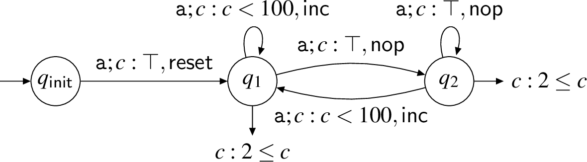
Example 2.
Consider a c-regex \(r={\texttt{{(aa*)\{2,100\}}}}\). In reality this is equivalent to the expression \({\texttt{{aaa*}}}\), but let us work out the counter use. For the CA \(M\) in [fig:ca-construction], \(L(r) = L(M)\), that is, \(M\) is equivalent to \(r\). The initial state always reads an \(a\) and goes to \(q_1\), which corresponds to being ‘at’ the \(a^*\) in the expression. There the options are: reading another \(a\) by using the Kleene star (going to \(q_2\) without changing the count \(c\)); reading another \(a\) by reentering the counter operation (incrementing \(c\), only possible if \(c<100\)); or accepting (possible only if \(c\ge 2\)). Note that \(\text{aaa} \in L(r)\). The following are the sequences of transition relations for \((q_{\mathsf{init}}, \{c: 0\}) \to_\texttt{aaa} (q, \alpha)\), for configs \((q, \alpha)\) reachable when reading \(\texttt{aaa}\).
\((q_{\mathsf{init}}, \{c: 0\}) \to_\texttt{a} (q_1, \{c: 1\}) \to_\texttt{a} (q_1, \{c: 2\}) \to_\texttt{a} (q_1, \{c: 3\})\)
\((q_{\mathsf{init}}, \{c: 0\}) \to_\texttt{a} (q_1, \{c: 1\}) \to_\texttt{a} (q_1, \{c: 2\}) \to_\texttt{a} (q_2, \{c: 2\})\)
\((q_{\mathsf{init}}, \{c: 0\}) \to_\texttt{a} (q_1, \{c: 1\}) \to_\texttt{a} (q_2, \{c: 1\}) \to_\texttt{a} (q_1, \{c: 2\})\)
\((q_{\mathsf{init}}, \{c: 0\}) \to_\texttt{a} (q_1, \{c: 1\}) \to_\texttt{a} (q_2, \{c: 1\}) \to_\texttt{a} (q_2, \{c: 1\})\)
We have that \(\texttt{aaa} \in L(M)\) since \((q_1, \{c: 3\}), (q_2, \{c: 2\})\) and \((q_1, \{c: 2\})\) are final configs.
2.3 Thompson-like matching algorithm↩︎
For a c-regex \(r\) and a string \(w \in A^*\), a Thompson-like matching algorithm decides whether \(w \in L(r)\), as follows: Consider a CA equivalent to \(r\), which we denote by \(M(r)\). A super-config of \(M\) refers to a set of configs of \(M(r)\). Next, we define the functional relations \(\Rightarrow_a\) and \(\Rightarrow_w\), over super-configs, for each super-config \(S\), character \(a \in A\) and \(w = a_1 a_2 \cdots a_n \in A^*\), as follows: \[\begin{align} S \Rightarrow_{(M, a)} \{ (q, \beta) \in Q \times {\mathsf{Assign}}(C) \mid \exists (p, \alpha) \in S: (p, \alpha) \to_{(M, a)} (q, \beta) \}, \\ (S \Rightarrow_{(M, w)} S_n) \iff (S \Rightarrow_{(M, a_1)} S_1 \Rightarrow_{(M, a_2)} S_2 \Rightarrow_{(M, a_3)} \cdots \Rightarrow_{(M, a_n)} S_n). \end{align}\] We write \(\Rightarrow_w\) for \(\Rightarrow_{(M, w)}\) when \(M\) is clear from the context.
Note that if \(\{ (p, \alpha) \} \Rightarrow_w T\), then \((p, \alpha) \to_w (q, \beta)\) if and only if \((q, \beta) \in T\). Finally, \(w \in L(M)\) if \(S_{\mathsf{init}}\Rightarrow_w S_n\), where \(S_{\mathsf{init}}:= \{(q_{\mathsf{init}}, \alpha_{\mathsf{init}})\}\) is the initial super-config, and \(S_n\) contains a final config.
Example 3. For the CA \(M\) in [fig:ca-construction], we have the following derivation of super-configs. \[\begin{align} \{ (q_{\mathsf{init}}, \{c: 0\}) \} &\Rightarrow_\texttt{a} \{ (q_1, \{c: 1\}) \} \\ &\Rightarrow_\texttt{a} \{ (q_1, \{c: 2\}), (q_2, \{c: 1\}) \} \\ &\Rightarrow_\texttt{a} \{ (q_1, \{c: 3\}), (q_2, \{c: 2\}), (q_1, \{c: 2\}), (q_2, \{c: 1\}) \}. \end{align}\] Note the correspondence between this derivation and the derivation sequences given in Example 2.
2.4 Flat counter automata↩︎
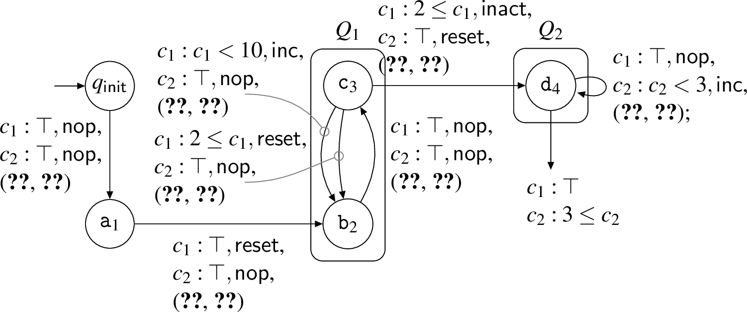
Next, we consider the position CA constructed from a c-regex \(r\) with the position construction as in [@GeladeGM12]; for example, [fig:position-construction] shows the position CA of the c-regex a((bc){2,10})+d{3,3}. The position CA of \(r\) has \(|r|_{\Sigma}\) states (where \(|r|_{\Sigma}\) denotes the number of predicates from \(\Sigma\) in \(r\)) and at most \({(|r|_{\Sigma})}^2\) transitions, and it has the properties outlined next (see [@HolikSTV23]). We begin with two required
definitions.
Definition 4 (See [@TuronovaHLSVV20]). For a counter variable \(c_i \in C\), the scope \(Q_i \subseteq Q\) of \(c_i\) is the smallest subset of \(Q\) defined inductively such that \(q\in Q_i\) if there exists a transition \((p, \sigma, \psi, \theta, q) \in \Delta\) such that either (1) \(\theta_i = {\mathsf{reset}}\), or (2) \(p \in Q_i\) and \(\theta_i \neq {\mathsf{inact}}\).
For each state \(q \in Q\), we denote by \(C_q := \{ c_i \in C \mid q \in Q_i \}\) the set of counter variables whose scope contains \(q\). Furthermore, we define \(Q_0 := Q \setminus \bigcup_{c_i \in C} Q_i\) as the set of states outside the scope of any counter. Consequently, \(C_q = \emptyset\) for any \(q \in Q_0\).
Definition 5 (Transition types). A transition type for a counter variable \(c_i \in C\) is a guard-action pair \((\psi(c_i), \theta(c_i))\) that falls into one of the following five types:
\((\top, {\mathsf{nop}})\),
\((\top, {\mathsf{reset}})\),
\((c_i < h_i, {\mathsf{inc}})\),
\((l_i \le c_i, {\mathsf{reset}})\), and
\((l_i \le c_i, {\mathsf{inact}})\).
The following two properties generalize the property presented in Appendix B.1 of Holı́k et al. [@HolikSTV23].
Property 1. For any transition \((p, \sigma, \psi, \theta, q) \in \Delta\) and counter variable \(c_i \in C\) of a position CA, the corresponding pair \((\psi(c_i), \theta(c_i))\) must be one of the five transition types in Definition 5, determined by the relation of state \(p\) and \(q\) to the counter’s scope \(Q_i\):
if \(p \notin Q_i \land q \notin Q_i\) then \((\psi(c_i), \theta(c_i))\) is [item:type-0];
if \(p \notin Q_i \land q \in Q_i\) then \((\psi(c_i), \theta(c_i))\) is [item:type-1];
if \(p \in Q_i \land q \in Q_i\) then \((\psi(c_i), \theta(c_i))\) is [item:type-0], [item:type-2] or [item:type-3].
if \(p \in Q_i \land q \notin Q_i\) then \((\psi(c_i), \theta(c_i))\) is [item:type-4].
Each of these follows naturally from the structure of the counter scopes. For example, in 1 we are outside the scope, so the counter has no effect, [item:type-0]; cases 2 and 3 enter and exit the scope. Only case 3 is somewhat complex, as the transition goes from a state inside the scope to another inside the scope. This can happen either without interacting with the counter operation at all, giving us [item:type-0]; by iterating the counter operation once, giving us [item:type-2]; or by exiting the counter operation and reentering it, using some enclosing closure, resetting the counter in [item:type-3].
Property 2. For any config \((q, \alpha)\) of the position CA and a counter variable \(c_i \in C\), \(\alpha(c_i) \ne 0\) if and only if \(q \in Q_i\).
We focus on the position CAs of flat c-regexes, referred to as flat CAs. In a flat CA, \(|C_q| = 1\) for \(q \notin Q_0\) and \(|C_q| = 0\) otherwise. In the flat case, we simplify the notation of a config \((q, \alpha)\) as follows: If \(q \in Q_i\) for some \(c_i \in C\), then the config is written as \((q, \alpha(c_i))\); if \(q \in Q_0\), it is written as \((q, 0)\). Note that every c-regex can be converted into a flat c-regex using counter-expansion [@Cox10] where we perform the expansion for all but one of the nested counters.
2.5 Counter configurations↩︎
Next, we describe the counting-set data structure that is used to represent a set of counter values assigned to a counter variable at each state, following Turoňová et al. [@TuronovaHLSVV20]; see also Le Glaunec et al. [@GlaunecKM23] for a related bit-parallel approach.
Definition 6. A counting-set, which is a representation based on an offset and an ordered list, is a tuple \(s = (o, \ell, l, h)\), where:
\(l \in {\mathbb{N}}_0\) and \(h \in {\mathbb{N}}_\infty\) with \(l \le h\) denote the interval \([l, h]\) representing the required number of repetitions;
\(o \in {\mathbb{N}}_0\) is the offset; and
\(\ell = {\langle {\ell_1, \ell_2, \ldots, \ell_n} \rangle}\) with \(|\ell| = n\) is an ordered list of strictly decreasing values with each \(\ell_i \in {\mathbb{N}}_0\) and \(o - \ell_i \in [0, h]\).
We only consider counting-sets that can be obtained from the initial counting-set, i.e.\((0, {\langle {0} \rangle}, l, h)\) (representing the set \(\{0\}\)), using the operations \({\mathsf{inc}}\), \({\mathsf{add}_1}\), \({\mathsf{merge}}\), defined below.
We use \(\ell_{\mathsf{head}}\) to denote the last element \(\ell_n\) of \(\ell\); when \(\ell\) is empty, we define \(\ell_{\mathsf{head}}:= \bot\). A counting-set \(s\) represents the set \(N_s:=\{ o - \ell_i \mid 1 \le i \le n \} \subseteq [0, h]\). With \(s=(o, \ell, l, h)\), we define the following operations on counting-sets, taking counting-sets as inputs to output a Boolean value for \({\mathsf{check}}\) and a new counting-set for \({\mathsf{inc}}\), \({\mathsf{add}_1}\) and \({\mathsf{merge}}\):
\({\mathsf{check}}(s) := [\ell_{\mathsf{head}}\ne \bot \land l \le o - \ell_{\mathsf{head}}]\); this checks whether \(N_s \cap [l, h] \ne \emptyset\);
\({\mathsf{inc}}(s) := (o + 1, \ell', l, h)\) represents \(1 + N_s\); when \((o + 1) - \ell_{\mathsf{head}}\le h\) (i.e.if \(\ell_{\mathsf{head}}\) is smaller than the upper bound \(h\)) \(\ell' := \ell\), otherwise \(\ell' := {\langle {\ell_1, \ell_2, \ldots, \ell_{n-1}} \rangle}\);
\({\mathsf{add}_1}(s) := (o, \ell', l, h)\) is defined when \(o>0\), and represents \(N_s \cup \{1\}\); we have \(\ell' := \ell\) if \(\ell_1 = (o-1)\), and \(\ell' := {\langle {o - 1, \ell_1, \ell_2, \ldots, \ell_n} \rangle}\), otherwise;
\({\mathsf{merge}}(s_1, s_2) := (o_1, \ell', l, h)\) represents the union of \(s_1=(o_1,\ell^1,l,h)\) and \(s_2=(o_2,\ell^2,l,h)\) for \(o_1 \ge o_2\), where \(\ell'\) is the result of merging \(\ell_1\) and the list \[{\langle {(o_1 - o_2) + \ell^2_1, (o_1 - o_2) + \ell^2_2, \ldots, (o_1 - o_2) + \ell^2_{\mathsf{head}}} \rangle},\] by also removing duplicates.
We can compute \({\mathsf{check}}(s)\), \({\mathsf{inc}}(s)\), and \({\mathsf{add}_1}(s)\) in time \(O(1)\). The operation \({\mathsf{merge}}(s_1, s_2)\) runs in \(O(o_2)\) time because \(o_2\) bounds (from above) both the size of \(\ell^2\) and the number of elements in \(\ell^1\) that must be processed during the merge. The operation \({\mathsf{merge}}(s_1, s_2)\) is defined as a destructive update where \(s_1\) consumes \(s_2\). Consequently, \(s_2\) becomes unavailable for further use. When computing \({\mathsf{merge}}(s_1, s_2)\), the number of visited elements in \(\ell_1\) and \(\ell_2\) is bounded by \(2 \cdot o_2\). Moreover, since the offset of \(s_2\) is \(o_2\), this implies that there were \(o_2\) calls to \({\mathsf{inc}}\) on \(s_2\) before merging. Combined with the fact that \(s_2\) is consumed by \({\mathsf{merge}}(s_1, s_2)\), this implies that the amortized time complexity of \({\mathsf{merge}}(s_1, s_2)\) is constant [@HolikSTV23]. 3 illustrates the structure of a counting-set.

Counting set automata use counting sets for efficient matching of c-regexes with CAs [@TuronovaHLSVV20; @GlaunecKM23; @HolikSTV23]. As a basis for our proposed matching algorithm, we describe counter-configurations, which we subsequently modify to obtain sparse counting-sets.
Definition 7. For a flat CA we work with the simplified configs \((q, n)\) introduced at the end of Section 2 (a flat CA has \(|C_q| \le 1\) for every state \(q\), so every assignment \(\alpha\) in a config reduces to a single value \(n = \alpha(c_i)\) if \(q \in Q_i\), and to \(n = 0\) if \(q \in Q_0\)). A counter configuration (c-config) is then a function \(f: Q {\,\rightharpoonup\,}{2^{{\mathbb{N}}_0}}\) that maps each state \(q\) to a set \(f(q)\) of counter values. A super-config \(S \subseteq Q \times {\mathbb{N}}_0\) is represented by the c-config \(f\) defined by \(f(q) := \{ n \in {\mathbb{N}}_0 \mid (q, n) \in S \}\), with \(f(q)\) undefined when no such pair occurs in \(S\).
Example 4. The following c- and super-configs represent the same set of configurations.
c-config \(f = \{ p\!: \{ 1, 2 \}, q\!: \{ 1, 2, 3 \}, r\!: \{ 1, 2, 3 \} \}\)
super-config \(S = \{ (p, 1), (p, 2), (q, 1), (q, 2), (q, 3), (r, 1), (r, 2), (r, 3) \}\)
Definition 8. Let \(S\) and \(T\) be super-configs of a flat CA such that \(S \Rightarrow_w T\) for some string \(w \in A^*\). If \(f\) and \(g\) are c-configs that represent \(S\) and \(T\), respectively, we write \(f \Rightarrow_w g\).
Note that the counter values associated with a state \(q\) are placed in the set \(f(q)\), which is represented using the counting-set structure. This representation allows a c-config to increase all values simultaneously via the operation \({\mathsf{inc}}\).
We define a flat c-regex \(r\) to be replicating if its corresponding position CA contains a state \(p \in Q_i\) with at least two outgoing transitions whose operations \(\theta(c_i)\) are from \(\{ {\mathsf{nop}}, {\mathsf{inc}}\}\) and whose predicates \(\sigma_1\) and \(\sigma_2\) are not disjoint (i.e., \({{[\![}{}{\sigma_1}{]\!]}{}} \cap {{[\![}{}{\sigma_2}{]\!]}{}} \ne \emptyset\)). 4 illustrates a CA of a replicating c-regex. In such a case, the matching algorithm in 5 needs to replicate the counting-set \(s\) in order to compute \(s'\). This replication requires time linear in the size of \(s\), which is at most \(H(r)\). Recall, \(H(r)\) denotes the largest finite bound in a counter range in \(r\) (i.e., every subexpression \(s^{\{l,h\}}\) has \(l\le H(r)\) and, if \(h\not =\infty\), then \(h\le H(r)\)). Next, we use this observation on the cost of replicating counting sets to analyse the time complexity of 5.
5 uses a counting-set data structure and c-configs to match an input string against a CA obtained by applying the position automaton construction to a flat c-regex. Notably, Line [line:condition-check] does not explicitly check guards for \({\mathsf{nop}}\) and \({\mathsf{inc}}\). This is unnecessary because (1) the guard component that corresponds to \({\mathsf{nop}}\) and \({\mathsf{inc}}\) is always \(\top\) and \(c_i < h_i\) by Property 1, and (2) counting-set’s \({\mathsf{inc}}\) operation implicitly filters out values that exceed the upper bound \(h_i\). For each state \(p\), the algorithm counts the number of outgoing transitions with \({\mathsf{nop}}\) or \({\mathsf{inc}}\) operations in Line [line:replication-count]. If more than one such transition exists, the corresponding counting-set is replicated in Line [line:replication]. Finally, as guaranteed by Property 1, the cases handled in Lines [line:transition-0], [line:transition-1], and [line:transition-2] are exhaustive and cover all possible transitions. Although we will not provide a formal correctness argument, note that the natural correctness invariant for 5 is the following: After processing the first i characters of the input, the c-config \(f\) maps each state \(q\) to exactly the set of counter values \(n\) such that the flat CA has a reachable config \((q,n)\) after that prefix.
For the proposition below to hold, we need to rewrite \(r^{\{l, \infty\}}\) as \(r^{\{l, l\}}r^*\). Alternatively, one may provide special treatment for the case \(r^{\{l, \infty\}}\) (not given in the pseudocode listed for Algorithm 5). For this, we split the transition for \((c_i < h, {\mathsf{inc}})\) of T4 in Definition 5 into \((c_i < l, {\mathsf{inc}})\) and \((c_i = l, {\mathsf{nop}})\) if \(h = \infty\), or by constraining the \({\mathsf{inc}}\) operation to have no effect once a counter reaches its lower bound \(l\) (if \(h = \infty\)).
Proposition 3 (See [@HolikSTV23]). For a flat c-regex \(r\) and a string \(w\), 5 (modified for the case \(r^{\{l, \infty\}}\)) on the position CA of \(r\) decides if \(w \in L(r)\) in \(O(H(r) \cdot (|r|_{\Sigma})^2 |w|)\)-time. Furthermore, if \(r\) is non-replicating, then 5 runs in \(O((|r|_{\Sigma})^2 |w|))\)-time.
![Figure 5: CA matching with counting-sets — adapted from Holík et al. [@HolikSTV23].](/article/2606.26679/_pdflatex/fwnmoavt.png "fig:")
3 Sparse counting-sets↩︎
Recall that the matching time complexity of replicating c-regexes depends on the maximum size of counting-sets. We propose a new data structure, the sparse counting-set, which stores only useful values. For example, for an expression \(E^{\{5,10\}}\) the sets \(\{4,5,6,7,8,9,10\}\) and \(\{4,10\}\) are indistinguishable under the counting operators; they both satisfy \({\mathsf{check}}\), and do so when applying \({\mathsf{inc}}\) up to six times, but stop satisfying \({\mathsf{check}}\) on a seventh \({\mathsf{inc}}\). This difference, at which any intermediary counter values become useless, will be used throughout this section. We let \(k=h-l+1\), with \(k=\infty\) when \(h=\infty\).
Definition 9. A sparse counting-set is a tuple \(s = (o, \ell, l, h)\) as in Definition 6, except it is produced from the initial counting-set using only the operations \({\mathsf{inc}}\), \({\mathsf{sparseAdd}_1}\) and \({\mathsf{sparseMerge}}\), defined next. Consequently, the CA matching algorithm with sparse counting-sets is exactly Algorithm 5, where the standard operations \({\mathsf{add}_1}\) and \({\mathsf{merge}}\) are replaced by their sparse counterparts \({\mathsf{sparseAdd}_1}\) and \({\mathsf{sparseMerge}}\), respectively.
\({\mathsf{sparseAdd}_1}(s) := (o, \ell'', l, h)\), where \(\ell''\) is constructed as follows. Let \({\mathsf{add}_1}(s) = (o, \ell', l, h)\) with \(\ell' = {\langle {\ell'_1, \ell'_2 \ldots, \ell'_{\mathsf{head}}} \rangle}\), noting that \(\ell'_1 = o-1\). Then, the ordered list \(\ell''\) is obtained by removing \(\ell'_2\) from \(\ell'\) if and only if \(\ell'_1 - \ell'_3 \le k\).
\({\mathsf{sparseMerge}}(s_1, s_2) := (o_1, \ell'', l, h)\), where \({\mathsf{merge}}(s_1, s_2) = (o_1, \ell', l, h)\) and \(\ell''\) is obtained from \(\ell'\) by iteratively checking triples \(\ell'_{i-1},\ell'_{i},\ell'_{i+1}\), in order of increasing \(i\), and removing \(\ell'_{i}\) if \(\ell'_{i-1}-\ell'_{i+1}\le k\). Assuming \(o_2\le o_1\), we may stop checking triples once \(\ell'_{i-1}<(o_1-o_2)\), or once we have inspected all triples in \(\ell'\).
As the definition implies, we will consider Algorithm 5 from here with the operations replaced by their sparse variants. The following lemmas are derived from the definitions of these operations.
Lemma 1. A sparse counting-set \(s = (o, \ell, l, h)\) with \(|\ell| \ge 3\), is such that the inequality \(\ell_i - \ell_{i+2} > k\) holds for any index \(i\).
Proof. We show this by induction. A sparse counting-set must be obtained using the operations \({\mathsf{inc}}\), \({\mathsf{sparseAdd}_1}\) and \({\mathsf{sparseMerge}}\). Only \({\mathsf{sparseAdd}_1}\) and \({\mathsf{sparseMerge}}\) lengthen a list \(\ell\). The lemma holds for the initial counting-set. The operation \({\mathsf{sparseAdd}_1}\) either prepends an element (precisely when doing so does not violate this inequality) or replaces the leading element. As the offset is monotonically increasing under all operators, this new leading element must be greater than or equal to the element it replaces, preserving this inequality. The operation \({\mathsf{sparseMerge}}\) directly removes the elements that violate this inequality by scanning triples in the merged list, left to right. Note that after adding \((o_1-o_2)\) to each element in the second list before merging, all elements of this list will be between \((o_1-1)\) and \((o_1-o_2)\), inclusive, so we can stop checking triples once \(\ell'_{i-1}<(o_1-o_2)\). ◻
Before stating the size bound, we record an invariant that simplifies the analysis. Although Definition 9 allows arbitrary sequences of \({\mathsf{inc}}\), \({\mathsf{sparseAdd}_1}\), and \({\mathsf{sparseMerge}}\), the sparse counting-sets that actually arise during a run of Algorithm 5 always satisfy \(o - \ell_i \geq 1\) for every index \(i\) (i.e., the value \(0\) occurs only in the bare initial counting-set \((0,\langle 0\rangle,l,h)\), which has \(|\ell| = 1\)).
The reason is as follows. \({\mathsf{sparseMerge}}\) is invoked only at line 25, in the branch \(c(q) \neq \bot \wedge \theta' \in \{{\mathsf{nop}},{\mathsf{inc}}\}\); by Property 1 this forces \(p, q \in Q_i\) for some counter \(c_i\), and a routine induction on the outer iteration shows that any counting-set stored at a state in some \(Q_i\) has an offset of at least \(1\). Propagating this through the operations: \(\mathsf{inc}\) strictly increments every \(v_i := o - \ell_i\), \({\mathsf{sparseAdd}_1}\) only ever prepends an element with \(v = 1\), and \({\mathsf{sparseMerge}}\) preserves the \(v\)-values of its operands. Since neither operand of a \({\mathsf{sparseMerge}}\) in Algorithm 9 is the bare initial counting-set, the invariant \(v_i \geq 1\) therefore propagates throughout. We will use this fact freely in Lemma 2 and Proposition 4.
Lemma 2. For a sparse counting-set \(s = (o,\ell,l,h)\) with \(h \geq 1\) arising during a run of Algorithm 1, the size \(|\ell|\) is bounded by \[H'(l, h) \;:=\; \begin{cases} \displaystyle 2\left\lceil \dfrac{h}{k+1} \right\rceil & \text{if } h \neq \infty,\\ 2 & \text{if } h = \infty. \end{cases}\]
Proof. For \(h = \infty\) we have \(k = \infty\), and \(|\ell| \leq 2\) is forced by Lemma 1.
For \(h \neq \infty\), let \(\ell = \ell_1, \dots, \ell_n\) and set \(v_i := o - \ell_i\), so \(v_1 < v_2 < \cdots < v_n\). The case \(n = 1\) is trivial since \(2\lceil h/(k+1) \rceil \geq 2\). So assume \(n \geq 2\); then \(s\) is not the bare initial counting-set (which has \(|\ell| = 1\)), and by the invariant noted above, we have \(v_i \geq 1\) for all \(i\). Hence \(v_i \in [1, h]\), and by Lemma 1 we have \(v_{i+2} - v_i \geq k + 1\).
Consider the odd-indexed subsequence \(v_1 < v_3 < \cdots < v_{2j-1}\), where \(j = \lceil n/2 \rceil\). Consecutive elements differ by at least \(k + 1\), so \(v_{2j-1} \geq v_1 + (j-1)(k+1) \geq 1 + (j-1)(k+1)\). Combined with \(v_{2j-1} \leq h\): \[(j-1)(k+1) \;\leq\; h - 1 \;\Longrightarrow\; j \;\leq\; \left\lfloor \frac{h-1}{k+1} \right\rfloor + 1 \;=\; \left\lceil \frac{h}{k+1} \right\rceil.\] The same argument applied to the even-indexed subsequence (whose smallest element is at least \(2\), giving \((i-1)(k+1) \leq h - 2\)) yields \(\lfloor n/2 \rfloor \leq \lceil h/(k+1) \rceil\). Summing gives \(n \leq 2\lceil h/(k+1) \rceil\). ◻
From the early stopping criteria in \({\mathsf{sparseMerge}}\), and using that, we merge sparse lists (i.e.we can apply the previous lemma to these two lists), we obtain the following proposition, which guarantees that the time complexity of \({\mathsf{sparseMerge}}\) improves on that of \({\mathsf{merge}}\) (assuming a large enough value of \(k\)), while preserving amortized constant time in the non-replicating case.
Proposition 4. For sparse counting-sets \(s_1, s_2\) arising during a run of Algorithm 5 with \(o_2 \leq o_1\), the computation of \(\mathsf{sparseMerge}(s_1, s_2)\) considers at most \(2\lceil o_2/(k+1) \rceil\) elements from each of the two lists to achieve the merge, and then investigates at most \(2 \cdot 2\lceil o_2/(k+1) \rceil\) triples from the merged list to restore sparsity.
Lemma 3. Let \(N_s, N_{s'} \subseteq {\mathbb{N}}_0\) be sets of counter values represented by a counting-set \(s\) and corresponding (i.e.produced with the corresponding sequence of sparse operations) sparse counting-set \(s'\), respectively. Then, \(N_{s'} \subseteq N_s\) and, for any \(n \in N_s \setminus N_{s'}\) with \(n \in [l,h]\), there exists \(n' \in N_{s'}\) such that \(n' \in [l, h]\). That is, \({\mathsf{check}}(s) = {\mathsf{check}}(s')\).
Sketch. The tuples \(s\) and \(s'\) clearly agree in offset, \(l\) and \(h\). Let \(\ell\) and \(\ell'\) be the ordered lists in \(s\) and \(s'\) respectively. By construction, \(\ell'\) is a subsequence of \(\ell\). We proceed by contradiction. Assume that \({\mathsf{check}}(s)\ne {\mathsf{check}}(s')\). Then we must have \({\mathsf{check}}(s)\) true and \({\mathsf{check}}(s')\) false, as \(s'\) represents a subset of \(s\). Then there is some value \(v\) in \(\ell\) that satisfies the check (i.e.\(l\le o-v\le h\)), which does not occur in \(\ell'\). The value \(v\) must have been removed either by \({\mathsf{sparseAdd}_1}\) or by \({\mathsf{sparseMerge}}\), but each removes a value only if it would otherwise occur in a context \(v',v,v''\) where \(v'-v''<k+1\). However, we must then have \(l\le o-v \le h\), \(o-v'<l\) and \(o-v''>h\), but then the difference between \(v'\) and \(v''\) would have to be at least \(h-l+2\), which causes a contradiction. ◻
Corollary 1. Let \(f\) be the c-config \(f\) of a flat CA representing the initial super-config. Given a string \(w \in A^*\), we compute a c-config \(g\) such that \(f \Rightarrow_w g\) using counting-set operations and replication of counting-sets. In parallel, we define another c-config \(g'\) obtained by applying the same procedure, but replacing each counting-set operation with its sparse counterpart. Then, \(g\) represents a final super-config if and only if \(g'\) represents a final super-config.
Proof. Follows from Lemma 3, with each sparse counting-set in the configuration acting indistinguishably from its non-sparse counterpart. ◻
Combined with Lemma 2, we derive the following definition of \(d\)-sparse. This property enables efficient matching with c-configs that use sparse counting-sets instead of regular counting-sets, which we refer to as sparse counter configurations (sc-configs).
Definition 10. A flat c-regex \(r\) is \(d\)-sparse if \(H'(l, h) \le d\) (with \(H'(l, h)\) as defined in Lemma 2) for every subexpression of the form \(s^{\{l, h\}}\) in \(r\).
Example 5. If all subexpressions of the form \(s^{\{l, h\}}\) of a c-regex \(r\) satisfy \(l = 0\) or \(h = \infty\), then the c-regex \(r\) is \(2\)-sparse.
With all this in hand, we can now state a bound on the membership problem using sparse counting-sets, stated in terms of \(d\). In many cases, \(d\) will be quite small, and in addition, in practice, this bound is pessimistic, as it accounts for the possibility of replicating sets linearly many times.
Theorem 5. Let \(r\) be a \(d\)-sparse c-regex. For a given string \(w \in A^*\), we can decide whether \(w \in L(r)\) in \(O(d \cdot (|r|_{\Sigma})^2 |w|)\)-time. If \(r\) is non-replicating, then the algorithm runs in \(O((|r|_{\Sigma})^2 |w|))\)-time.
Proof. The automaton representing \(r\) still has \((|r|_{\Sigma})^2\) as the number of transitions: While counting operations create additional transitions (e.g., the two transitions from \(c_3\) to \(b_2\) in Figure [fig:position-construction]), \(r\) being flat means any pair of states belongs to at most two counter scopes, making only a constant number of counter operations possible on transitions between that pair. The factor \(d\) bounds the size of the representation of a sparse counting-set, allowing copying and/or merging sets within this bound. ◻
Remark 6. For the sake of a simpler presentation, we did not discuss an optimization where sparse counting-sets for ranges like \(r^{\{0,h\}}\), \(r^{\{1,h\}}\), or \(r^{\{l, \infty\}}\) only need to store a single value.
4 Experimental evaluation↩︎
We evaluate the efficiency of our sparse counting-set approach against baselines. Efficiency is quantified by the total computation steps required for symbol evaluations, guard checks, and counting-set operations. This includes (1) the number of processed counter values during \({\mathsf{merge}}\) operations and (2) the number of counter values involved in the replication of counting-sets. Performance is assessed through targeted analyses of hand-crafted patterns and large-scale evaluations on the Polyglot and Snort3 under adversarial and random input scenarios.
4.1 Results on targeted regular expressions↩︎
Manually designed c-regexes have one of the following properties: (a) non-replicating, (b) 2-sparse, or (c) neither. We evaluate and compare four distinct methods—counter-expansion followed by Thompson NFA matching (c-expansion), Thompson-like matching with super-configs (super-config), standard counter-configs (c-config), and counter-configs with sparse counting-sets (sc-config). For the c-expansion method, the position CA construction is applied to the counter-expanded regex, yielding a standard position NFA where all guards are \(\psi(c) = \top\) and actions are \(\theta(c) = {\mathsf{nop}}\).


Figure 7: A comparison of the number of computation steps for our manually designed c-regexes, each matched against strings of the form \(\texttt{a}^\text{k}\). The x-axis indicates the length of the input
string, which corresponds to the value k in each pattern’s counting operator..
The results in 7 highlight the advantages of our sparse counting-set approach. First, both the counter-expansion and super-config methods fail to achieve linear-time matching. As shown in 7 (b), the standard c-config approach is also limited, achieving linear-time performance only on non-replicating c-regexes. However, by incorporating the sparse counting-set, we extend this capability to achieve linear-time
matching for replicating c-regexes that are \(d\)-sparse for a bounded \(d\). The reason our sparse counting-set provides no advantage in 7 (c) is
explained by Lemma 2. For a counting operator such as {k,k}, the upper bound \(H'(l,h)\) of the number of values
in a sparse counting-set becomes equal to an upper bound \(h\) for the non-sparse one, as \(h - l + 1\) is simply \(1\). As both bounds are k,
any potential benefit from sparsity is lost.
Furthermore, our experimental results demonstrate that for cases with a finite upper bound \(h\) in a counter operation \(r^{\{l, h\}}\), the performance of the super-config method is within a constant factor of the counter-expansion approach. This result aligns with the theoretical explanation—each config \((q,n)\) in the super-config approach is equivalent to a state in the position NFA generated by counter-expansion. The constant factor difference arises from the elimination of guards and actions in the position NFA of the expanded regex.
4.2 Results on real-world regular expressions↩︎
Next, we use c-regexes from two sources: the Polyglot regex corpus by Davis et al. [@DavisMCSL19] and the Talos LightSPD Snort3 ruleset (snapshot-31470). Polyglot contains 511,196
patterns (30,833 with counters) and Snort3 contains 9,755 patterns (2,837 with explicit counters). Table 1 summarizes the structural properties of these patterns, determined via static analysis of their position
counting automata.
We also compute the distribution of \(H'(l,h)\) for 64,792 and 4,734 individual counter operators found in flat regexes from Polyglot and Snort3, respectively, to assess the practical bound of the parameter d on matching performance. Figure 8 illustrates histograms of lower-bound \(l\) and upper-bound \(h\) of counter operators and the size \(H'(l,h)\) of sparse counting-sets in our approach.
| Property | Polyglot | Snort3 | ||
|---|---|---|---|---|
| 1-1 (r)2-3 Total with counters | 30,833 | (100%) | 2,837 | (100%) |
| Flat (depth \(d = 1\)) | 29,911 | (97.0%) | 2,749 | (96.9%) |
| Replicating | 319 | (1.0%) | 79 | (2.8%) |
| 2-sparse | 15,161 | (49.2%) | 1,300 | (45.8%) |
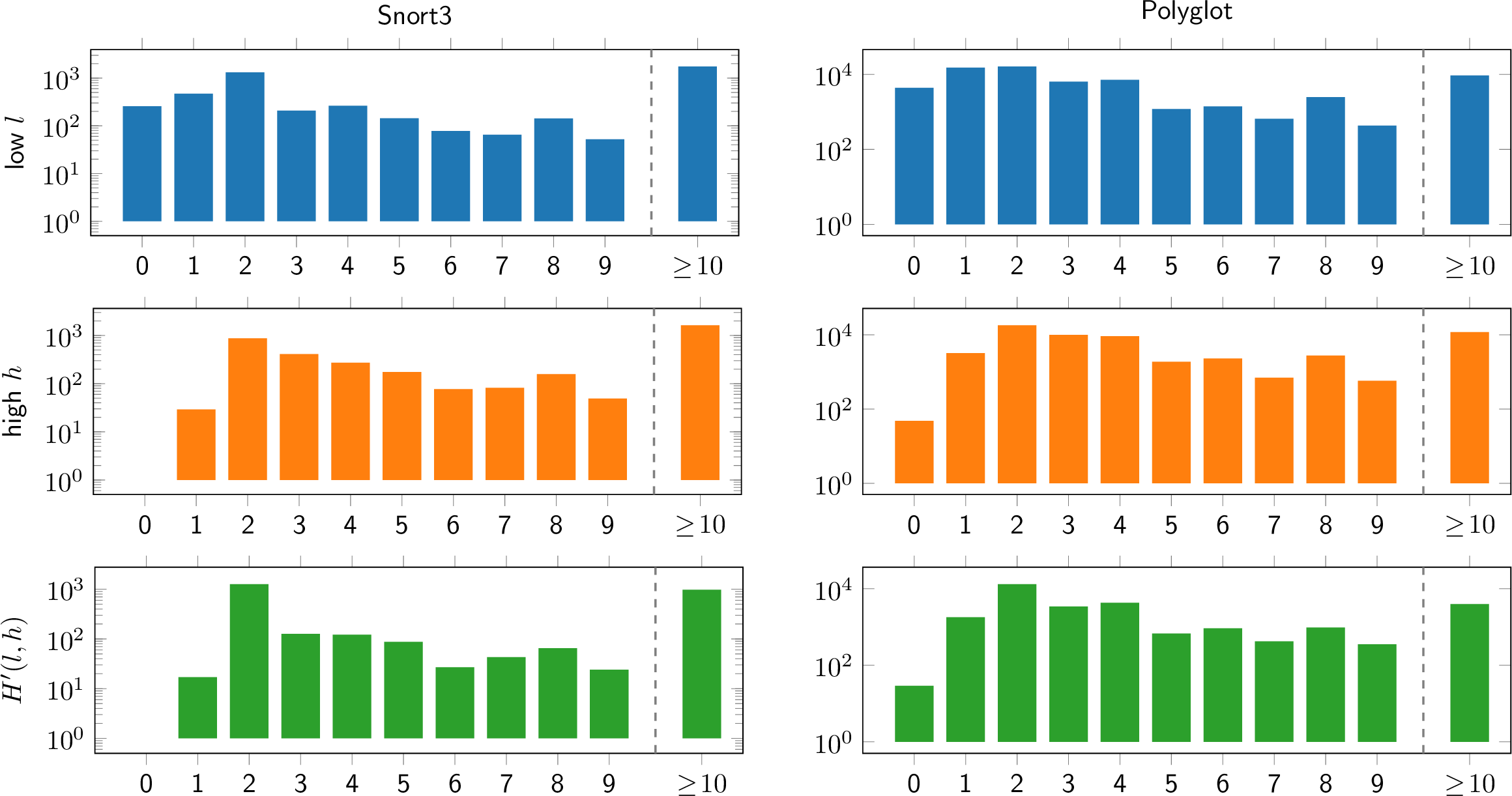
The bottom row of 8 is the empirical distribution of \(H'(l,h)\), whose per-pattern maximum is exactly the \(d\) of 5. In both corpora, the mass concentrates at small values, with only a short tail at \(H'(l,h) \ge 10\); this is driven by the commonly occurring unbounded ranges, which give \(H'(l,h) = 2\) by Lemma 2. Hence, for most real-world patterns, \(d\) is a small constant, and the \(O(d \cdot (|r|_\Sigma)^2 |w|)\) bound is within a small factor of the non-replicating \(O((|r|_\Sigma)^2 |w|)\).
Our experiments evaluate the robustness of our approach by conducting two parallel sets of experiments simulating adversarial and random input scenarios. In both cases, we simulated a partial matching scenario by wrapping each pattern \(r\) as .*(r).* to generate corresponding input strings. Our final dataset is filtered to include only c-regexes that meet three criteria: they (a) contain at least one counting operation, (b) are supported by our
implementation, and (c) have a successfully generated test case.
4.2.0.1 Adversarial (9):
EvilStrGen [@SuHLCG24] is designed to generate test cases that maximize the number of matching steps. EvilStrGen was configured to assume a non-backtracking engine and to generate string lengths of approximately 1,000. In summary, we use 10,108 and 611 c-regexes from the Polyglot and Snort3 datasets for the experiments with EvilStrGen, respectively.
4.2.0.2 Random (10):
We simulate a random-input scenario by generating matched inputs with Xeger2. We use Xeger with its default limit \(10\), which decides the maximum number of repetitions for Kleene star, plus, and counting operators with infinite upper bounds. For the experiments with Xeger, we use 10,141 and 620 c-regexes from the Polyglot and Snort3 datasets, respectively.


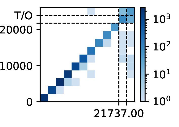


Figure 9: Comparisons of matching steps with input strings generated by EvilStrGen, presented as a sequence of 2D histograms. Each plot is labeled in a “Method 1 vs. Method 2” format, where the x-axis represents the step count for the first method and the y-axis for the second with the same scale. The color of each cell represents the number of such c-regex input string pairs. The second last line denotes the 99th percentile, and cases above (or to the right of) the “T/O” label timed out after one second..


Figure 10: Comparisons of matching steps with input strings generated by xeger, using the same experimental setup as in 9. The 2D histograms show pairwise comparisons of the four
methods, with cell color indicating the density of test cases..
5 Conclusion and future work↩︎
We introduced c-configs, a formalization of on-the-fly matching with counting-set automata [@HolikSTV23]. Based on this formalization, we presented a representation of super-configs as sparse counting-sets, minimizing the number of counter values that are required to be tracked.
One can utilize counter expansion to convert non-flat c-regexes into flat c-regexes. The choice of which counting operator to expand influences the resulting expression. For instance, the c-regex \(({\texttt{{a\{2,3\}b)\{2,2\}}}}\) can be expanded as either \({\texttt{{(aaa?b)\{2,2\}}}}\) or \({\texttt{{(a\{2,3\}b)(a\{2,3\}b)}}}\). Determining which expansion form leads to more efficient CA-based matching is left as future research. We would also like to explore the possibility of generalizing the (sparse) counting-set data structure to support non-flat c-regexes.
Acknowledgements↩︎
The authors thank Rick Bower and River Martin for their detailed review of the experimental results.
[@*]
Authors are listed alphabetically. While this work represents a collaborative effort, Sicheol Sung served as the lead author.↩︎