A geometric approach to inner problems associated with exponentially small splitting phenomena in local bifurcations
June 25, 2026
Abstract
In this paper, we study analytic nonlinear partial differential equations for \(\mathbf{y}=\mathbf{y}(x,\theta)\in \mathbb{C}^n\) of the form \(x^2 \mathbf{y}'_x(1+\mathcal{O}(x)) + \mathbf{y}'_\theta+x \mathbf{A} \mathbf{y} = \mathcal{O}(x^2)\), \(()'_z=\frac{\partial}{\partial z}\), \(z=x,\theta\), with \(x\in \mathbb{C}\) and \(\theta\in \mathbb{C} /(2\pi \mathbb{Z})\) denoting the independent variables. We show that solutions are \(1\)-sums (with respect to \(x\)) of Fourier series with coefficients of type Gevrey-\(1\). The motivation for studying these equations is that so-called inner problems, associated with two-dimensional formal connections in unfoldings of local bifurcations, can be brought into this form (by looking for invariant manifolds in blowup coordinates). In the present paper, we give two examples: The zero-Hopf bifurcation and the resonant Hopf-Hopf bifurcation, both in the reversible settings. Importantly, these inner problems are given by the unperturbed problem (i.e. at the bifurcation) and the invariant manifolds are expressed directly in phase space (through blowup coordinates associated with the local bifurcation). This contrasts the Lazutkin-based formulation of inner problems which is based upon a blowup of singularities (with respect to complex time) of approximate solutions; for local bifurcations this requires (artificial) coordinate transformations. We solve the PDE by extending the Banach-convolution-algebra-approach to Borel-Laplace by Bonckaert and De Maesschalck (2008) to account for analytic Fourier series. In further details, we apply the Borel transform with respect to \(x\) (keeping \(\theta\) fixed) and solve the resulting equation in an appropriate Banach space of Fourier series with coefficients that have exponential growth in the Borel plane. The solutions of the PDE are then obtained through application of the Laplace transformation. We see our results as prerequisites for the (forthcoming) phase space-analysis of exponentially small phenomena associated with local bifurcations, without following Lazutkin’s approach. Keywords. Inner problems, exponentially small splitting, invariant manifolds, blowup, Zero-Hopf bifurcation, Hopf-Hopf bifurcation, reversible systems, center manifolds.
Mathematics Subject Classification. 34C23, 34D15, 34C45, 37G10
1 Introduction↩︎
In this paper, we consider the following partial differential equation for \(\mathbf{y}=\mathbf{y}(x,\theta)\): \[\begin{align} \label{eq:main} x^2 \mathbf{y}'_x (1+xF_0+x^2 F_1(x,\mathbf{y},\theta))+\mathbf{y}'_\theta+ x \mathbf{A} \mathbf{y} = x^2 \mathbf{G}_1(x,\mathbf{y},\theta),\quad x\in B_\kappa,\,\theta\in \mathbb{T}_\zeta, \end{align}\tag{1}\] with \(()'_z=\frac{\partial}{\partial z}\), \(z=x,\theta\). Here \(F_0\in \mathbb{C}\), and \[\begin{align} \label{eq:Adiag} \mathbf{A}= \operatorname{diag}(\lambda^1,\ldots,\lambda^n)\in \mathbb{R}^{n\times n},\quad \forall\,j\in \{1,\ldots,n\}\,:\,\lambda^j>0. \end{align}\tag{2}\] Importantly, \[F_1:B_\kappa\times B_{\kappa}^n\times \mathbb{T}_\zeta\rightarrow \mathbb{C},\quad and\quad \mathbf{G}_1:B_\kappa\times B_\kappa^n\times \mathbb{T}_\zeta\to \mathbb{C}^n,\] with \(B_\kappa^n\subset \mathbb{C}^n\), \(n\in \mathbb{N}\), denoting the open ball of radius \(\kappa>0\) centered at the origin, are assumed to be analytic functions. For simplicity, we write \(B_\kappa:=B_\kappa^1\) throughout. Finally, we note that \[\mathbb{T}_\zeta:=\left\{\theta\in \mathbb{C}/(2\pi \mathbb{Z})\,:\,0\le \operatorname{Im}(\theta)\vert <\zeta\right\},\] with \(\zeta>0\).
We emphasize that solutions of (1 ) define invariant manifold solutions of \[\label{eq:mainvf} \begin{align} \dot{x} &= x^2 (1+xF_0+ x^2 F_1(x,\mathbf{y},\theta)),\\ \dot{\mathbf{y}} & = x\left(- \mathbf{A} {\mathbf{y}} +x \mathbf{G}_1(x,{\mathbf{y}},\theta)\right),\\ \dot{\theta} &=1. \end{align}\tag{3}\] The main motivation for looking at (3 ) is that such systems appear as so-called inner problems associated with exponentially small phenomena related to formal connections in formal normal forms of local bifurcations. In this paper, we will give two main examples: The two-dimensional formal connections in the zero-Hopf bifurcation and the resonant Hopf-Hopf bifurcation. We believe that the reversible setting is the interesting case and will therefore restrict attention to reversible systems.
Our first main result on (1 ) is the following:
Theorem 1. Let \(S^{\pm}(\delta,\chi)\subset \mathbb{C}\) denote the local open sectors, centered along the positive (\(+\)) respectively negative \((-\)) real axis, of radius \(\delta>0\) and opening \(\pi+\chi\in (\pi,2\pi)\): \[\begin{align} \label{eq:Spm} S^{\pm}(\delta,\chi)=\left\{x\in \mathbb{C}\,:\,0< \vert x\vert< \delta\,and \, \vert \operatorname{Arg}(\pm x)\vert< \frac{\pi+\chi}{2}\right\}, \end{align}\qquad{(1)}\] see Fig. [fig:Spm]. Fix any \(\chi\in (0,\pi)\). Then for \(\delta>0\), \(\xi>0\), both small enough, there exists two analytic solutions: \[\begin{align} \mathbf{y}^\pm\,:\,S^\pm \times \mathbb{T}_\xi \to \mathbb{C}^n, \end{align}\] respectively, of (1 ). In particular, upon writing \(\mathbf{y}^\pm\) as Fourier series: \[\begin{align} \mathbf{y}^\pm(x,\theta) =: \sum_{\alpha\in \mathbb{Z}} \mathbf{y}_\alpha^\pm(x) {\mathrm e}^{i\alpha\theta}, \end{align}\] respectively, we have that the Fourier coefficients \[\begin{align} \mathbf{y}_\alpha^\pm(x) =\mathcal{O}(x{\mathrm e}^{-\vert \alpha\vert\xi}) ,\quad \alpha\in \mathbb{Z},\,x\in S^\pm, \end{align}\] (the estimate being uniform) are \(1\)-sums of a Gevrey-\(1\) series: \[\begin{align} \label{eq:gevrey1series} \mathbf{y}_\alpha(x) \sim_1 \sum_{\beta=1}^\infty \mathbf{y}_{\alpha,\beta} x^\beta\quad \forall\,\alpha\in \mathbb{Z}, \end{align}\qquad{(2)}\] (the series being independent of \(\pm\)) in the directions defined by \(S^\pm\), respectively.
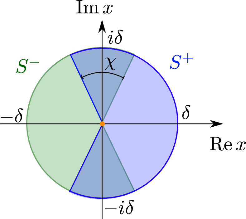
Figure 1: Illustration of the local sectorial domains \(S^\pm\) (with radius \(\delta>0\) and opening \(\pi+\chi\in (\pi,2\pi)\)..
Recall that a Gevrey-\(1\) series \(\widetilde{W}\in \mathbb{C}[[x]]\) is said to be \(1\)-summable in the direction \(\varphi\in \mathbb{T}:=\mathbb{R}/(2\pi \mathbb{Z})\) if (a) the Borel transform \(w\mapsto \widehat W(w)\in \mathbb{C},\,w\in B_\kappa\subset \mathbb{C}\), of the series (which is a convergent series, see [1] and Remark 11 below) can be endlessly continued to an analytic function \(\widehat W^\varphi\), along the ray defined by \(w=r{\mathrm e}^{i\varphi}\), \(r\ge 0\), and (b) it is of at most exponential growth of order \(1\) along this ray, i.e. \[\begin{align} {\mathrm e}^{-\eta \vert w\vert} \vert \widehat W^\varphi(w)\vert =\mathcal{O}(1) \quad for\quad w\to \infty{\mathrm e}^{i\varphi}, \end{align}\] for some \(\eta>0\) large enough. Then the Laplace-transform \(W^\varphi:=\mathcal{L}^{\varphi}[\widehat W^\varphi]\) is well-defined on a local sector \(S^\varphi\) centered along \(\varphi\) and with opening greater than \(\pi\). \(W^\varphi\) is called the \(1\)-sum of \(\widetilde{W}\) in the direction \(\varphi\) and it is unique (due to the opening being greater than \(\pi\), see Watson’s lemma [1]). In particular, \(W^\varphi\) is Gevrey-\(1\) asymptotic to \(\widetilde{W}\) (which we write as \(W^\varphi\sim_1\widetilde{W}\)) on \(S^\varphi\). For further details, we refer to [1], see also Section 4. Now, the formal Gevrey-\(1\) series in (?? ) is in general divergent (since the manifolds will be center-like manifolds) and the difference \[\begin{align} \Delta \mathbf{y} (x,\theta):= \mathbf{y}^+(x,\theta)-\mathbf{y}^-(x,\theta)\sim_1 0,\quad x\in S^+\cap S^-, \end{align}\] uniformly with respect to \(\theta\in \mathbb{T}_\xi\), is therefore generically nonzero, see e.g. [1], [2]. (The divergence can be understood in different ways but one possible characterization is through singularities of the Borel transform, see [3], [4].) Notice that \(S^+\cap S^-\) is the union of two sectors of the complex plane centered along the directions defined by \(\pm \frac{\pi}{2}\), each with opening \(\chi\in (0,\pi)\).
In the following, we define \[\begin{align} q^{-\mathbf{A}}:=\operatorname{diag}(q^{-\lambda^1},\cdots,q^{-\lambda^n})\in \mathbb{C}^{n\times n},\quad q\ge 0, \end{align}\] recall (2 ).
Theorem 2. Consider \(x=ip\) with \(p\in [0,p_0]\) with \(p_0>0\) small enough. Then there exists a constant vector \[\begin{align} \mathbf{C}_{-1}\in \mathbb{C}^n, \end{align}\] such that \[\begin{align} \Delta \mathbf{y}(ip,\theta) = {\mathrm e}^{-\frac{1}{p}-iF_0\log p}p^{-\mathbf{A}} \left(\mathbf{C}_{-1}{\mathrm e}^{-i\theta}+ p \mathbf{R}(p,\theta)\right)\quad \forall\,p\in (0,p_0],\,\theta\in \mathbb{T}_\xi.\label{eq:Deltay} \end{align}\qquad{(3)}\] Here \(\mathbf{R}\,:\,[0,p_0]\times \mathbb{T}_\xi\to \mathbb{C}^n\) is \(C^\infty\)-smooth with respect to \(p\) and analytic with respect to \(\theta\in \mathbb{T}_\xi\). In particular, \[\begin{align} \mathbf{R}(p,\theta) = \sum_{\alpha\in \mathbb{Z}} \mathbf{R}_\alpha (p){\mathrm e}^{i\alpha\theta}, \end{align}\] with \(\vert \mathbf{R}_\alpha(p)\vert = \mathcal{O}({\mathrm e}^{-\xi \vert \alpha\vert})\) uniformly with respect to \(p\).
There is obviously a similar expression for the difference for \(p<0\). It takes the same form as (?? ) after replacing \((p,F_0,\theta,\mathbf{C}_{-1})\) by \((-p,-F_0,-\theta,\mathbf{C}_{1})\). In particular, if the equations are real-analytic (which is often the interesting case), then the expression for \(p<0\) is simply obtained from (?? ) by conjugation (so that \(\mathbf{C}_{1}=\overline{\mathbf{C}}_{-1}\)). Moreover, if (?? ) with \(\alpha=-1\) is convergent then \(\Delta \mathbf{y}_{-1} = 0\). Hence \(\mathbf{C}_{-1} \ne 0\) implies that (?? ) with \(\alpha=-1\) is divergent. At this stage, we do know if the other direction also holds true so that “if (eq. 2 ) with \(\alpha=-1\) is divergent then \(\mathbf{C}_{-1} \ne 0\)”.
We will study (1 ) using Borel-Laplace, extending the Banach-convolution-algebra-approach of [5]. We believe that Borel-Laplace is the natural framework in problems with exponentially small slitting because the beyond all order phenomena are intrinsically related to the divergence of formal series solutions. Borel-Laplace deals with the resummation of such series.
1.1 A new perspective on inner problems↩︎
In this paper, we also use (1 ) as a platform to promote a new perspective (initiated in [6]) on inner problems and more broadly on exponentially small splitting phenomena in local bifurcations.
Inner problems are known to be central in the rigorous description of exponentially small phenomena in analytic singular perturbation problems. Following the work of Lazutkin [7], [8], these problems are “suitable approximations” of (invariant manifold) solutions near singularities of unperturbed (or approximate) solutions, see also [9]. They are typically derived through a blowup of poles and appropriate scalings of the variables.
For the purpose of this introduction, we will explain such derivation within the context of the real-analytic unfolding of the zero-Hopf bifurcation with the normal form: \[\label{eq:zerohopf0} \begin{align} x' &=-x^2+\epsilon-a (y^2 +z^2) + F(x,y,z,\epsilon),\\ y'&= b x y -z+G(x,y,z,\epsilon),\\ z'&= b x z+ y+H(x,y,z,\epsilon), \end{align}\tag{4}\] see [10] and [6]. We will then subsequently explain a different perspective on the inner problem.
Notice in comparison with [6] that we have replaced their \((x,y,z,\mu)\) by \((-x,z,y,\epsilon)\) in (4 ). Moreover, we restrict attention to the reversible case (setting \(\sigma=0\) in [6]), assuming that \[\begin{align} \begin{cases} F(-x,-z,-y,\epsilon)=F(x,y,z,\epsilon)\\ G(-x,-z,-y,\epsilon)=H(x,y,z,\epsilon) \end{cases}\quad \forall\,(x,y,z)\in B_\tau^3, \,\epsilon\in (-\epsilon_0,\epsilon_0), \end{align}\] with \(\tau>0\), \(\epsilon_0>0\), both small enough. It then follows that \((x(t),y(t),z(t))\) is a solution if and only if \((-x(-t),-z(-t),-y(-t))\) is a solution. We let \[\begin{align} \mathcal{S}\,:\,(x,y,z)\mapsto (-x,-z,-y),\label{eq:symmetry0} \end{align}\tag{5}\] denote the associated symmetry. The functions \(F,G\) and \(H\) are assumed to be real-analytic, defined in a neighborhood of \((x,y,z,\epsilon)=(0,0,0,0)\) in \(\mathbb{C}^4\), and each function is third order: \[\begin{align} \label{eq:Wthird} W(x,y,z,\epsilon) = \mathcal{O}(\vert (x,y,z,\epsilon)\vert^3),\quad W=F,G,H, \end{align}\tag{6}\] with respect to \((x,y,z,\epsilon)\to (0,0,0,0)\). We are mainly interested in \[a>0,\quad b>0.\] The parameter \(\epsilon\sim 0\) is the unfolding parameters. (Recall that the general non-reversible case has two unfolding parameters, see [10]). For \(\epsilon=0\), we have a locally unique singularity at the origin with eigenvalues \(0,\pm i\) of the linearization.
Consider now the change of coordinates \((x_2,y_2,z_2)\mapsto (x,y,z)\) defined by \[\begin{align} \label{eq:x2y2z20} \begin{cases} x=r_2 x_2, \\ y=r_2 y_2, \\ z=r_2 z_2,\\ \epsilon = r_2^2. \end{cases} \end{align}\tag{7}\] This brings the system into the following slow-fast form \[\label{eq:zerohopf20} \begin{align} \dot{x}_2 &=-x_2^2+1+ a (y_2^2+z_2^2)+r_2 F_2(x_2, y_2, z_2,r_2),\\ r_2 \dot{y}_2&=r_2 b x_2y_2+ z_2+r_2^2 G_2(x_2, y_2, z_2,r_2),\\ r_2 \dot{z}_2&= r_2 b x_2 z_2-y_2+r_2^2 H_2(x_2,y_2,z_2,r_2), \end{align}\tag{8}\] where \(\frac{d}{dt}=\dot{(\cdot)}=r_2^{-1} (\cdot )'\) and \[\begin{align} W_2(x_2, y_2, z_2,r_2^2):=r_2^{-3} W(r_2 x_2,r_2 y_2,r_2 z_2,r_2^2),\quad W=F,G,H, \end{align}\] which are well-defined by (6 ). For \(r_2\to 0\), we obtain the reduced problem: \[\begin{align} \label{eq:reduced} \dot{x}_2 &= -x_2^2+1, \end{align}\tag{9}\] on the normally elliptic critical manifold defined by \((y_2,z_2)=(0,0)\). The reduced problem (9 ) has a homoclinic orbit \(\gamma_0\) with the following parametrization: \[\begin{align} \label{eq:unperturbed_sol} x_2 = \tanh (t),\quad t\in \mathbb{R}. \end{align}\tag{10}\] For \(b>0\), a simple calculation (based upon the implicit function theorem) shows that there are two saddle-focus equilibria \(E_2^\pm(r_2)\) near \((\pm 1,0,0)\) for all \(0<r_2\ll 1\). However, for \(r_2>0\) but small, the unperturbed homoclinic \(\gamma_0\) will in general break up, see [10]. The splitting is beyond all orders and exponentially small with respect to \(r_2\to 0\) (i.e. \(\epsilon\to 0\) cf. (7 )).
The central observation of Lazutkin is that the splitting of the invariant manifolds is not beyond all orders near the singularities \(t_2=\pm \frac{i\pi}{2}\) (closest to the real axis) of the unperturbed connection. Although Lazutkin’s work centered around the standard map, this framework has subsequently proven to be very powerful for the description of exponentially small phenomena in a range of different analytic differential equations, see e.g. [11]–[16] and references therein.
To describe the splitting of the one-dimensional invariant manifolds in the zero-Hopf bifurcation, the authors of [10] derive an inner problem in the following way: Let \(s\) be defined as \[t=t(s):=\frac{i\pi}{2}+r_2 s.\] Notice that this is a blowup of \(t=\frac{i\pi}{2}\) for \(r_2=0\). Through (10 ) and (7 ) we obtain a change of coordinates \((s,y,z)\mapsto (x_2,y_2,z_2)\) defined by \[\begin{align} \label{eq:x2ts} x_2 = \tanh (t(s)) = {\operatorname{coth}(r_2 s)}=\frac{1}{r_2 s} \left(1+\mathcal{O}(r_2)\right),\quad s\ne 0, \end{align}\tag{11}\] which brings the equations (4 ) into the following form: \[\label{eq:inner_temp} \begin{align} \left(-r_2^2 \operatorname{coth}^2(r_2 s)-a(y^2+z^2)+ F\right)\frac{dy}{ds}&=-r_2^2 \operatorname{csch}^2(r_2 s)\left(-z+b{r_2 \operatorname{coth}(r_2 s)}y + G\right),\\ \left(-r_2^2 \operatorname{coth}^2(r_2 s)-a(y^2+z^2)+ F\right)\frac{dz}{ds}&=-r_2^2 \operatorname{csch}^2(r_2 s)\left(y+b{r_2 \operatorname{coth}(r_2 s)}z + H\right). \end{align}\tag{12}\] The inner problem of [10] is then the \(r_2 \to 0\) limit of (12 ): \[\label{eq:inner_fucked} \begin{align} \left(-s^{-2} -a(y^2+z^2)+ F\right)\frac{dy}{ds}&=-s^{-2} \left(-z+bs^{-1}y + G\right),\\ \left(-s^{-2} -a(y^2+z^2)+ F\right)\frac{dz}{ds}&=-s^{-2} \left(y+bs^{-1}z + H\right), \end{align}\tag{13}\] with \(s\ne 0\) and where \(W=W(s^{-1},y,z,0)\), \(W=F,G,H\). Here we have used that \[\begin{align} \label{eq:sech_limit} r_2 \operatorname{coth}(r_2 s) \to s^{-1},\quad r_2 \operatorname{csch}(r_2 s) \to s^{-1}, \end{align}\tag{14}\] as \(r_2\to 0\), \(s\ne 0\). In [10] the authors are concerned with invariant manifolds of (13 ) for \(s\to\pm \infty\) in certain sectors of the complex plane.
We now notice the following simple fact: The system (13 ) is equivalent with (4 ) for \(\epsilon = 0\): \[\label{eq:inner} \begin{align} x' &=-x^2-a (y^2 +z^2) + F(x,y,z,0),\\ y'&=b x y - z+G(x,y,z,0),\\ z'&= b x z + y+H(x,y,z,0), \end{align}\qquad{(4)}\] through the change of coordinates defined by \(x=s^{-1}\). Notice in particular, that by (10 ) \(x_2(t(s)) = \frac{1}{r_2 s} +\mathcal{O}(1)\) so that \[x=s^{-1} \quad as\quad r_2=\sqrt{\epsilon} \to 0, \,s\ne 0,\] recall (7 ).
In conclusion, the inner problem associated with (4 ) is just the unperturbed system. This will also be the case in our subsequent examples, and we believe that this a general phenomena. (We believe that it is hard to make rigorous statements of this kind. We also remark that this connection between the inner problem and the unperturbed system has also been noted by experts in the field, see e.g. [17] and [18].) Therefore it seems unnatural to follow the approach of Lazutkin for these kind of local bifurcation problems.
Notice that for (?? ), we look for invariant manifolds in the \((x,y,z)\)-phase space as graphs over \(x\in S^{\pm}\). The existence of such manifolds follows from the theory of generalized saddle-nodes, see e.g. [5]. Indeed, the linearization of (?? ) has eigenvalues \(0,\pm i\) and the invariant manifolds are center-like manifolds, being graphs over the zero eigenspace along the sectors \(x\in S^\pm\).
In [5], generalized saddle-nodes are described through Borel-Laplace. Since their invariant manifolds are intrinsically related to summability, it is (in the opinion of the author) the most natural approach to study such manifolds. In this paper, we will extend the Borel-Laplace approach of [5] to study the PDE (1 ). We believe that this extension is interesting in itself. We are confident that the approach can be extended to inner problems associated with maps (as in [18]).
1.2 Exponentially small splitting↩︎
Let us briefly explain how the inner problem in [10] relates to the exponentially small splitting of the one-dimensional connection (10 ) for \(\epsilon\to 0\): In line with Lazutkin’s approach, the authors of [10] first parameterize the one-dimensional stable and unstable manifolds of \(E_2^\pm\) in terms of \(t\in \mathbb{C}\) (using (11 ) as a change of coordinates \(t\mapsto x_2 = \tanh (t)\)) up close to the poles \(t=\pm \frac{i\pi}{2}\) for all \(0<\epsilon\ll 1\). (Notice that \(\tanh(t)\in (-1,1)\) for \(t\in \mathbb{R}\), and consequently additional adjustments have to made to ensure that \(E_2^\pm \in (-1,1)\), see [10].) Near the poles, the authors show that the invariant manifolds are given by the invariant manifolds of (?? ) to leading order. The authors refer to this as matching (on an \(\epsilon\)-dependent domain) of the “outer expansion” (away from the poles) and the “inner expansion” (on the blowup of the pole). Since the invariant manifolds for \(s\to \pm \infty\) are different in general (which is quantified in terms of a Stokes constant in [10]), this essentially leads to a splitting of the invariant manifolds for \(\epsilon>0\) small enough. To determine an asymptotic formula for the real splitting for \(t=0\) (corresponding to \(x_2=0\)), a linear boundary value problem is derived. In this way, the separation close to the pole is carried down to the real axis; in this step one also uses the fact that the equations are real analytic.
In [6], the present author provided an alternative more geometric approach to the splitting problem of the one-dimensional invariant manifolds of \(E_2^\pm\). This approach builds upon the fact that the inner problem is just the unperturbed system and therefore works exclusively in the (complex) phase space. Importantly, the author treats the scaling (7 ) as a \(\breve \epsilon=1\)-chart of an associated blowup transformation: \[\begin{align} \label{eq:blowup0} r\ge 0,\,(\breve x,\breve y,\breve z,\breve \epsilon) \in \mathbb{S}^4\,\mapsto \begin{cases} x = r\breve x,\\ y = r\breve y,\\ z=r\breve z,\\ \epsilon = r^2 \breve \epsilon.\end{cases} \end{align}\tag{15}\] (Strictly, speaking the authors use a slightly different scaling, but this is a technicality and not really important here.) First, the author describes the stable and unstable manifolds of \(E_2^\pm\) in the coordinates \((x_2,y_2,z_2)\) as graphs over \(x_2\) in compacts subsets for \(0<r_2\ll 1\). The invariant manifolds are then extended by the flow to \(x=\mathcal{O}(1)\) by working in the separate coordinate chart defined by \(\breve x=1\): \[\begin{align} \begin{cases} x = r_1,\\ y = r_1 y_1,\\ z=r_1 z_1,\\ \epsilon = r_1^2 \epsilon_1.\end{cases} \end{align}\] The coordinates \((r_1,y_1,z_1)\) are natural coordinates for the parametrization of the invariant center-like manifolds of (?? ) within \(\epsilon=0\) (corresponding to \(\epsilon_1=0\)). Indeed, in these coordinates it is elementary to bring (?? ) into the form \[\begin{align} r_1^2 \frac{d\zeta_1}{dr_1} =\begin{pmatrix} 0 & -1\\ 1 & 0 \end{pmatrix} \zeta_1+\mathcal{O}(\vert(r_1,\zeta_1)\vert^2), \end{align}\] with \(\zeta_1=(y_1,z_1)\). Moreover, it follows from the change of coordinates between \(\breve x=1\) and \(\breve \epsilon=1\): \[\begin{align} \begin{cases} r_1 =r_2x_2,\\ y_1 = y_2x_2^{-1},\\ z_1 = z_2 x_2^{-1},\\ \epsilon_1 = x_2^{-2}, \end{cases} \end{align}\] that the invariant manifolds of the \(\breve \epsilon=1\)-chart are also (partially) visible in the \(\breve x=1\)-chart (for \(r_1=\mathcal{O}(\sqrt{\epsilon})\) and with \(x_2\) bounded uniformly away from zero). The results of [6] show that the extensions of the local stable and unstable manifolds of \(E_2^\pm\) are \(\mathcal{O}(r_2)\)-close to the invariant manifolds of the unperturbed system (?? ) within appropriate small but compact sets of \(x\in \mathbb{C}\) that are uniformly bounded away from \(x=0\). The paper [6] also presents an alternative geometric approach for the difference by deriving a Fenichel normal form, see [19]. In this way, the results of [6] directly relate the exponentially small splitting with the lack of analyticity of the center-like manifolds of (?? ).
We emphasize that [6] works directly in phase space, with the outer (inner) problem of the Lazutkin-based approach in [10] corresponding to \(x=\mathcal{O}(\sqrt \epsilon)\) (\(x=\mathcal{O}(1)\), respectively). (From the perspective of blowup, it feels most natural to refer to the unperturbed system (4 ) as the outer system and (8 ) as inner system; after all, in order to obtain (8 ) from (4 ) we zoom in on \((x,y,z,\epsilon)=(0,0,0,0)\) through the scaling (7 ). Unfortunately, within the Lazutkin-framework it is the other way around. To avoid (further) confusion, we stick to the terminology from Lazutkin in this paper.) It is by now well-established that blowup is a powerful systematic technique for connecting different scaling regimes in dynamical systems, see e.g. [20]–[23]. We believe that [6] supports this further. In this reference, we also see that blowup allows for a very detailed information about the \(\epsilon\)-dependency (in line with previous work on blowup, see e.g. [24] and [25] more broadly) of the splitting of the one-dimensional invariant manifolds of the zero-Hopf.
1.3 Discussion↩︎
The papers [26], [27] demonstrate a different connection between splitting phenomena and lack of analyticity of center manifolds. In particular, in [26] the authors consider the analytic unfolding of the planar saddle-node bifurcation and study the properties of the analytic weak-stable manifold as the system approaches the saddle-node (coming from the side of the bifurcation where a saddle and a node co-exist). The problem is singular in the sense that the analytic weak-stable manifold is only well-defined when the node is nonresonant and these resonances accumulate as the system approaches the bifurcation. However, the main result of [26] shows (under some hypothesis which by the subsequent work [4] can be relaxed) that if a certain Stokes-like constant is nonzero then the center manifold at the bifurcation is nonanalytic. Moreover, it is demonstrated that this quantity (qualitatively) determines the position of the analytic weak-stable manifold. In particular, it is shown (under the assumption of a nonzero Stokes constant) that the analytic weak-stable manifold never coincides with the invariant manifolds of the saddle. Although this problem is clearly different from the zero-Hopf bifurcation in many aspects, it does bear some important similarities. For example, [26] treats the unperturbed problem as an inner-like system having a center manifold (in the usual sense of a partially hyperbolic singularity). As for the zero-Hopf in [6], this manifold is then connected to an invariant manifold (the analytic weak-stable manifold of the nonresonant node) of the system in the scaled (blowup) coordinates.
In [28], the present author applies the geometric method from [6] (on the one-dimensional splitting associated with the zero-Hopf bifurcation) to a general class of co-dim \(k\), \(k\ge 3\), (non-reversible) zero-Hopf bifurcations. Although these bifurcations are more esoteric, the paper [28] perhaps illustrates the method in [6] more clearly, by also making connections to Stokes and anti-Stokes curves (drawing inspiration from [29]–[31]).
Looking ahead, the geometric viewpoint in [6], [28] opens up for potential applications in general problems where the explicit time dependency of unperturbed solutions are unknown. However, a central component in the development of phase space space methods for the splitting of more complicated connection problems, is to describe invariant manifolds of the unperturbed systems directly in phase space. We address this issue in the present paper by studying existence of two-dimensional invariant manifolds of (3 ).
1.4 The zero-Hopf and Hopf-Hopf bifurcations↩︎
In the present paper, we will demonstrate that the inner problems associated with the two-dimensional formal connections in the following local bifurcations, can be brought into the form (3 ):
The zero-Hopf in \(\mathbb{R}^3\) (see \(\Gamma_0\) in Fig. [fig:x2rho2] and Section 2 for further details).
The reversible and resonant Hopf-Hopf bifurcation in \(\mathbb{R}^4\) (see \(\Gamma_0\) in Fig. [fig:hopfhopf] and Section 3 for further details).
For the reversible zero-Hopf singularity, we will work with the normal form (4 ), whereas for the reversible and resonant Hopf-Hopf bifurcation in \(\mathbb{R}^4\), we will consider the following normal form: \[\label{eq:nfhopfhopf0} \begin{align} \dot{x} &=-(1+\Omega)y+z+F,\\ \dot{y} &=(1+\Omega)x+w+G,\\ \dot{z} &= -(1+\Omega)w+\Gamma x+H, \\ \dot{w} &=(1+\Omega )z+\Gamma y+J, \end{align}\tag{16}\] with \[\begin{align} W=W(x,y,z,w,\epsilon)=\mathcal{O}(\vert (x,y,z,w,\epsilon)\vert^5),\quad W=F,G,H,J, \end{align}\] and where \[\begin{align} \nonumber \begin{cases} \Gamma(\rho^2,L,\epsilon) = \epsilon - b \rho^2 +c L,\\ \Omega(\rho^2 ,L,\epsilon)=\alpha \epsilon + \beta \rho^2 +\gamma L, \end{cases} \end{align}\] for \[\begin{align} \rho^2:=x^2+y^2,\,L:=wx-yz, \end{align}\] see [32]. (Notice that in comparison with [32], we write their \((A,B)\) as \((x+iy,z+iw)\) to obtain a real normal form.) Here \(\epsilon\sim 0\) is the unfolding parameter.
Notice that for \(\epsilon=0\), the linearization of the origin has eigenvalues \(\pm i\) each with algebraic multiplicity \(2\) and geometric multiplicity \(1\). This bifurcation is also known as the \(1:1\) resonance bifurcation or \((i\omega)^2\) in symbols, see [32]. Importantly, the system (16 ) is assumed to be reversible with respect to the symmetry: \[\begin{align} \mathcal{S}\,:\,(x,y,z,w)\mapsto (x,-y,-z,w). \end{align}\]
This type of bifurcation occurs in the stationary generalized Swift-Hohenberg equation: \[\begin{align} \kappa u^2 -u^3 -(1+\partial_x^2)^2 u =\epsilon u, \end{align}\] see [15], and in travelling waves of the fifth order KdV-equation, see [33]. Both cases have a Hamiltonian structure, see also [34] for a Hamiltonian analysis of the Swift-Hohenberg equation (and generalizations hereof). We do not cover Hamiltonian systems but are confident that our approach carries over completely analagously.
In the context of (16 ), we again define an inner problem as the unperturbed system, i.e. (16 ) with \(\epsilon=0\).
For further details, we refer to Section 2 and Section 3 where we also compare with the Lazutkin-based approach for the inner problem.
We summarize our findings on the two examples as follows:
Proposition 3. There exist changes of coordinates (of blowup-type) that bring the inner problems (i.e. the unperturbed problems with \(\epsilon=0\)) associated with (4 ) (for any \(b\in \mathbb{R}\setminus [-1,0]\), \(a\in \mathbb{R} \setminus\{0\}\)) and (16 ) (for any \(b\in \mathbb{R}\setminus\{0\}\)) into the normal form (3 ).
In turn, we have the following corollaries of Theorem 1:
Proposition 4. Consider (4 ) with \(\epsilon=0\) for any \(b\in \mathbb{R}\setminus [-1,0]\), \(a\in \mathbb{R} \setminus\{0\}\), in the cylindrical coordinates \((x,\rho,\theta)\) defined by \[\begin{align} \begin{cases} y = \rho \cos \theta,\\ z = \rho \sin \theta. \end{cases} \end{align}\] Then there are invariant manifolds of the graph form \[\begin{align} \rho = x\Phi^\pm (x,\theta),\quad x\in S^\pm,\quad \theta\in \mathbb{T}_\xi, \end{align}\] where \(\Phi^\pm\,:\,S^\pm \times \mathbb{T}_\xi\to \mathbb{C}\) with \[\Phi^\pm(0,\theta) \equiv i \sqrt{\frac{1+b}{a}},\] are \(1\)-sums (with respect to \(x\), uniformly with respect to \(\theta\in \mathbb{T}_\xi\)) of a Gevrey-\(1\) formal series along the directions defined by \(x\in S^\pm\), respectively.
In the following, we let \(\upsilon S^\pm\), \(\upsilon\in \mathbb{C}\), denote the sets \[\begin{align} \upsilon S^\pm : =\{x\in \mathbb{C}\,:\,\upsilon^{-1}x\in S^\pm\}, \end{align}\] recall (?? ).
Proposition 5. Consider (16 ) with \(\epsilon=0\) for any \(b\in \mathbb{R}\setminus\{0\}\) in the coordinates \((\rho,\theta,\psi,L)\) defined by \[\begin{align} \nonumber \begin{cases} x = \rho \cos \theta,\\ y =\rho \sin \theta,\\ z =\psi \cos \theta - L\rho^{-1} \sin \theta,\\ w = \psi \sin \theta+ L\rho^{-1} \cos \theta. \end{cases} \end{align}\] Let \[\begin{align} \upsilon:=i^{-1}\sqrt{\frac{2}{b}}. \end{align}\] Then there are invariant manifolds of the graph form \[\begin{align} \begin{cases} \psi = \rho^2 \Phi^{\psi,\pm} (\rho,\theta),\\ L = \rho^3\Phi^{L,\pm}(\rho,\theta), \end{cases}\quad \quad \rho \in \upsilon S^\pm,\quad \theta\in \mathbb{T}_\xi, \end{align}\] where \(\Phi^{q,\pm}\,:\,\upsilon S^\pm \times \mathbb{T}_\xi\to \mathbb{C}\) with \[\begin{cases}\Phi^{\psi,\pm}(0,\theta) \equiv i \sqrt{\frac{b}{2}},\\ \Phi^{L,\pm}(0,\theta)\equiv 0,\end{cases}\] are \(1\)-sums (with respect to \(x\), uniformly with respect to \(\theta\in \mathbb{T}_\xi\)) of a Gevrey-\(1\) formal series along the directions defined by \(x\in \upsilon S^\pm\), respectively.
Proposition 3 is a consequence of Lemma 2 and Lemma 4 below. These results are each obtained in the same way, by working in charts associated with the problem-dependent blowups. In further details, we first show the existence of formal series solutions. We then truncate this series and subsequently apply a (separate) blowup (following the preparation of the generalized saddle-nodes in [5]).
Proposition [proposition:zerohopf] and Proposition 5 follow from more detailed statements below (in charts), see Proposition 8 respectively Proposition 10. For further details, see Section 2 and Section 3.
We view these results as prerequisites for our upcoming treatment of the associated exponentially small splitting phenomena in these problems as \(\epsilon\to 0\).
1.5 Outline↩︎
The paper is organized as follows. In Section 2, we first consider the two-dimensional formal connection of (4 ). We derive the associated inner problem by following Lazutkin’s approach and show that the system is equivalent with the unperturbed system. Moreover, we show that the unperturbed system (in polar coordinates) can be written in the form (3 ). Next in Section 3, we perform a similar analysis on the reversible and resonant Hopf-Hopf bifurcation with normal form (16 ). In particular, we again identify two-dimensional formal connections and bring the unperturbed system (which agrees with Lazutkin’s version of the inner problem) into the form (3 ). In both cases, blowup plays a crucial role.
In Section 4, we then review the Banach-convolution-algebra-approach to Borel-Laplace by Bonckaert and De Maesschalck, see [5], and extend it so that it can be applied to (1 ) (with the \(\theta\)-dependency). In Section 5, we then recast (1 ) into an equation in the Borel-plane for the Borel transform \(\widehat{\mathbf{y}}\) of \(\mathbf{y}\). We solve this equation in the appropriate Banach space of exponentially growing solutions along an infinite sector, using the theory from Section 4 and a fixed-point argument. The Laplace transformation \(\mathcal{L}^\varphi[\widehat{\mathbf{y}}]\) of \(\widehat{\mathbf{y}}\) then solves (1 ) along sectors (defined by \(\varphi\)). In this way, we prove Theorem 1 (taking \(\varphi=0\) and \(\varphi=\pi\)). Finally, in Section 6 we study the difference \(\Delta \mathbf{y}(x,\theta)\) for \(x\in S^+\cap S^-\) and prove Theorem 2. Our approach for the difference is also geometric (using invariant manifolds).
2 The reversible zero-Hopf bifurcation↩︎
In this section, we describe the inner problem associated with the two-dimensional formal connection between the saddle-focus singularities \(E_2^\pm\) of the reversible zero-Hopf bifurcation (8 ) and bring it into the general form (3 ). In order to introduce the two-dimensional formal connection for (8 ), we start by ignoring the higher order terms of (4 ): \[\label{eq:zerohopf0trunc} \begin{align} x' &=-x^2+\epsilon-a (y^2 +z^2),\\ y'&= bx y -z,\\ z'&= bx z+ y, \end{align}\tag{17}\] and write the resulting system in polar coordinates \((x,\rho,\theta)\) defined by \[\begin{align} \label{eq:polar} \begin{cases} y = \rho \cos \theta,\\ z =\rho\sin \theta. \end{cases} \end{align}\tag{18}\] This gives the following system: \[\label{eq:xrho} \begin{align} x' &=-x^2+\epsilon -a \rho^2,\\ \rho' &=bx\rho,\\ \epsilon' &=0, \end{align}\tag{19}\] and \(\dot{\theta} = 1\), which decouples. In anticipation of the blowup: \[\begin{align} \label{eq:blowup0polar} r\ge 0,\,(\breve x,\breve \rho,\breve \epsilon)\in \mathbb{S}^3\mapsto \begin{cases} x =r \breve x,\\ \rho = r\breve \rho,\\ \epsilon = r^2\breve \epsilon \end{cases} \end{align}\tag{20}\] recall (15 ), we have also augmented an equation for \(\epsilon\). We are primarily interested in the case \[a>0,\quad b>0.\]
In the \(\breve\epsilon=1\)-chart associated with (20 ), having the chart-specific coordinates \((x_2,\rho_2,r_2)\) defined by \[\begin{align} \begin{cases} x =r_2 x_2,\\ \rho =r_2 \rho_2,\\ \epsilon =r_2^2, \end{cases} \end{align}\] we find that \[\label{eq:x2rho2} \begin{align} \dot{x}_2 &=-x_2^2+1 -a \rho_2^2,\\ \dot{\rho}_2 &=bx_2\rho_2, \end{align}\tag{21}\] and \(\dot{r}_2=0\) after dividing the right hand side by the common factor \(r_2\). We then notice that \((x_2,\rho_2)=(\pm 1,0)\) (corresponding to \(E_2^\pm\)) are hyperbolic saddles of (21 ) for any \(b>0\), with the linearization having eigenvalues \[\begin{align} \mp 2,\quad \pm b, \end{align}\] respectively. The set \(\gamma_0\) defined by \(\rho_2=0,\,x_2\in (-1,1)\), is therefore a heteroclinic connection (corresponding to (10 )) for any \(b>0\), see Fig. [fig:x2rho2]. On the other hand for \(a>0\) and \(b>0\), we also have local stable and unstable manifolds of \((x_2,\rho_2)=(\mp 1,0)\), respectively, transverse to \(\rho_2=0\) that also coincide (due to the symmetry \(\mathcal{S}\)) to form a separate heteroclinic connection \(\Gamma_0\) contained within \(\rho_2>0\). We illustrate this situation in Fig. [fig:x2rho2]. An easy computation shows that the connection \(\Gamma_0\) takes the following graph form: \[\begin{align} \label{eq:Gamma0eqn} \Gamma_0\,:\,\rho_2 = \sqrt{\frac{1+b}{a}(1-x_2^2)},\quad x_2\in (-1,1). \end{align}\tag{22}\] Finally, we note that on \(\Gamma_0\) we have \[\begin{align} \dot{x}_2 &=b (x_2^2-1), \end{align}\] and from this we deduce that the heteroclinic connection \(\Gamma_0\) has the following time parametrization: \[\begin{align} \label{eq:unperturbed_sol2} \begin{cases} x_2(t) = -\tanh(bt),\\ \rho_2(t) =\sqrt{\frac{1+b}{a}} \operatorname{sech}(bt), \end{cases} \end{align}\tag{23}\] with poles closest to the real axis given by \(t=\pm \frac{i\pi}{2b}\).
Remark 6. It is easy to see that the higher order terms in (4 ), ignored in (17 ), lead to regular perturbations of (49 ) of order \(\mathcal{O}(r_2)\) in the \((x_2,\rho_2,\theta)\)-coordinates (in compact domains with \(\rho_2\) bounded uniformly away from zero). The symmetry \(\mathcal{S}\) takes the following form \((x_2,\rho_2,\theta)\mapsto (-x_2,\rho_2,-\theta-\frac{\pi}{2})\) in the \((x_2,\rho_2,\theta)\)-coordinates. From this one can deduce the existence of two symmetric homoclinic orbits for all \(0<r_2\ll 1\) (due to the intersection of stable and unstable manifolds with \(x_2=0\), \(\theta = -\frac{\pi}{4}+n\pi\), \(n\in \mathbb{Z}\), being the fixed-point set of the symmetry). The interesting problem (from the perspective of exponentially small phenomena) is then an asymptotic formula for the splitting of tangent spaces and whether there are other non-symmetric homoclinic orbits. This question is addressed in [17] (also within the non-reversible case). In further details, [17] gives an asymptotic formula for the difference between the two-dimensional stable and unstable invariant manifolds within \(\{x_2=0\}\). We aim to study this problem using the geometric approach of the present paper and [6], [28] in future work.
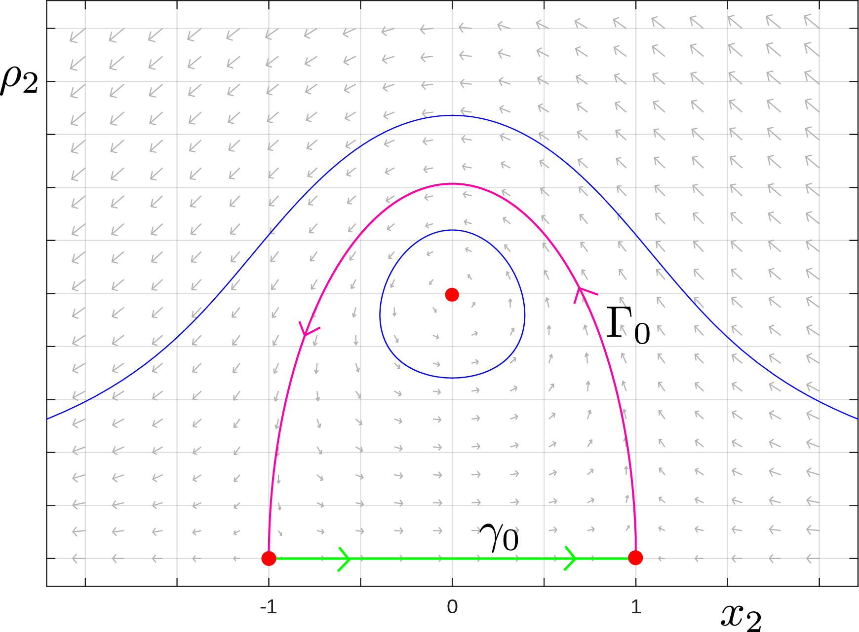
Figure 2: Phase portrait of (21 ) for \(a>0\), \(b>0\). There are two heteroclinic connections \(\gamma_0\subset \{\rho_2=0\}\) and \(\Gamma_0\subset \{\rho_2>0\}\)..
We first follow Lazutkin’s approach for the derivation of an inner problem associated with \(\Gamma_0\) (see also [17]): Let \(s\) be such that \[\begin{align} \label{eq:ts}t=t(s):=\frac{i\pi}{2b}+r_2 \frac{s}{b}. \end{align}\tag{24}\] Then (23 ) becomes \[\begin{align} \label{eq:unperturbed_sol2s} \begin{cases} x_2(t(s)) = - \coth(r_2 s),\\ \rho_2(t(s)) =-i \sqrt{\frac{1+b}{a}}\operatorname{csch}(r_2 s), \end{cases} \end{align}\tag{25}\] We write this set in the \((x,\rho,\theta)\) coordinates defined by \((y,z)=\rho (\cos(\theta),\sin(\theta))\), recall (7 ): \[\begin{align} \begin{cases} x(t(s)) := r_2 x_2(t(s))\to -s^{-1},\\ \rho(t(s)) :=r_2 \rho_2(t(s))) \to -i\sqrt{\frac{1+b}{a}} s^{-1}, \end{cases} \end{align}\] as \(r_2 \to 0\), \(s\ne 0\). It follows that \[\begin{align} \rho = i\sqrt{\frac{1+b}{a}} x,\quad x\in \mathbb{C},\label{eq:unperturbed_sol20} \end{align}\tag{26}\] is an invariant manifold solution of (19 ) within \(r_2=0\). This can also be directly verified. There is obviously also an invariant manifold of the form \(\rho = -i\sqrt{\frac{1+b}{a}} x\). Notice moreover that the equation for \(\Gamma_0\) in (22 ) becomes \[\begin{align} \rho = \sqrt{\frac{1+b}{a}(r_2^2-x^2)}\to \pm i\sqrt{\frac{1+b}{a}}x\quad for\quad r_2 \to 0, \end{align}\] in the \((x,\rho)\)-coordinates. In conclusion, (26 ) is an approximation (nonuniform) of the invariant manifolds of (17 ) in the phase space variables \((x,\rho,\theta)\). (In the language of [17] (inspired by Lazutkin) it is an approximation of the invariant manifolds near the poles of the unperturbed solution (23 )).
This motivates the definition of the inner problem associated with \(\Gamma_0\) as the unperturbed problem (?? ) (with \(F, G, H\) added) written in polar coordinates: \[\label{eq:inner2} \begin{align} x' &=-x^2 - a \rho^2 + F,\\ \rho' &=b x \rho + G\cos \theta+H\sin \theta,\\ \theta' &=1+\rho^{-1}\left(-G\sin \theta+H\cos \theta\right), \end{align}\tag{27}\] where \(W=W(x,\rho \cos \theta,\rho \sin \theta,0)\), \(W=F,G,H\). In contrast to the inner problem associated with \(\gamma_0\) (treated in the introduction), we are now interested in manifolds that are graphs over \((x,\theta)\) of the form: \[\begin{align} \rho =\rho(x,\theta)=\pm i\sqrt{\frac{1+b}{a}}x (1+\mathcal{O}(x))\quad for\quad x\to 0.\label{eq:rho_ansatz_zerohopf} \end{align}\tag{28}\]
It is natural to study (27 ) in the coordinates \((r_1,\rho_1)\) of the \(\breve x=1\)-chart defined by \[\begin{align} \label{eq:entry1} \begin{cases} x = r_1,\\ \rho = r_1 \rho_1,\\ \epsilon = r_1^2 \epsilon_1. \end{cases} \end{align}\tag{29}\] Indeed, (26 ) takes the following form \[\begin{align} \rho_1= i\sqrt{\frac{1+b}{a}},\,r_1\in \mathbb{C},\,\epsilon_1=0, \end{align}\] in these coordinates. The change of coordinates defined by (29 ) brings (27 ) into the following form:\[\label{eq:entry1eqns} \begin{align} \dot{r}_1 &=r_1^2 \left(-1-a \rho_1^2 + r_1 F_1\right),\\ \dot{\rho}_1 &=r_1\rho_1\left(1+b+a\rho_1^2+r_1 F_1\right)+r_1^2 G_1 \cos \theta+r_1^2 H_1\sin \theta,\\ \dot{\theta} &=1+\rho_1^{-1} r_1^2 \left(-G_1\sin \theta+H_1\cos \theta\right), \end{align}\tag{30}\] within \(\epsilon_1=0\). Here the functions \(W_1=W_1(r_1,\rho_1,\theta)\), \(W=F,G,H\), are defined as \[\begin{align} \label{eq:W1defn} W_1(r_1,\rho_1,\theta):=r_1^{-3}W(r_1,r_1\rho_1\cos \theta,r_1\rho_1\sin \theta,0),\quad r_1\in B_\tau,\,\rho_1\in D,\,\theta\in \mathbb{T}_\xi, \end{align}\tag{31}\] with \(D\subset \mathbb{C}\) a fixed compact set bounded away from zero and \(\tau>0\), \(\xi>0\), both small enough. Notice in particular that each \(W_1\) extends analytically to \(r_1=0\) by (6 ). For (30 ) we are interested in invariant manifold solutions \(\rho_1=\rho_1(r_1,\theta)\) with \[\begin{align} \rho_1(0,\theta) =\pm i\sqrt{\frac{1+b}{a}}. \end{align}\] We will only focus on “\(+\)”. The system (30 ) is reversible with respect to the symmetry \[\begin{align} \mathcal{S}_1\,:\, (r_1,\rho_1,\theta)\mapsto (-r_1,\rho_1,-\theta+\pi/2).\label{eq:symmetryzerohopf} \end{align}\tag{32}\] This is derived from (5 ) using (18 ) and (29 ), see also Remark 6.
We note that the inner problem associated with the connection \(\Gamma_0\) is cast in a different form in [17] (since the authors follow Lazutkin’s approach). Here the authors again view the \(x_2\)-solution of the truncated system: \(x_2 = -\tanh(bt)\) as a change of coordinates \(t\mapsto x_2\) and zoom in on the pole at \(t=\frac{i\pi}{2b}\) (\(t=-\frac{i\pi}{2b}\) is related by conjugation) through (24 ). This brings (4 ) into the following form \[\begin{align} \left(-r_2^2 \operatorname{coth}^2(r_2 s) +r_2^2 -a \rho^2 + F\right) \frac{d\rho}{ds} &=r_2^2 \operatorname{csch}^2(r_2 s) \left( b\rho\left(- r_2 \operatorname{coth}(r_2 s) +r_2 \sigma\right) + G\cos \theta+H\sin \theta\right),\\ \left(-r_2^2 \operatorname{coth}^2(r_2 s) +r_2^2 -a \rho^2 + F\right) \frac{d\theta}{ds} &=r_2^2 \operatorname{csch}^2(r_2 s) \left( 1 +\rho^{-1}\left(- G\sin \theta+H\cos \theta\right)\right), \end{align}\] with \(W=W(-r_2 \coth(r_2 s),\rho \cos \theta,\rho \sin \theta,r_2^2)\), \(W=F,G,H\). The inner problem (based upon Lazutkin’s approach) is then defined as the \(r_2\to 0\) limit: \[\label{eq:inner_fucked2} \begin{align} \left(-s^{-2} -a \rho^2 + F\right) \frac{d\rho}{ds} &=s^{-2} \left( b\rho s^{-1} + G\cos \theta+H\sin \theta\right),\\ \left(-s^{-2} -a \rho^2 + F\right) \frac{d\theta}{ds} &=s^{-2} \left( 1 +\rho^{-1}\left(- G\sin \theta+H\cos \theta\right)\right), \end{align}\tag{33}\] with \(s\ne 0\) and where we redefine \(W=W(-s^{-1},\rho \cos \theta,\rho \sin \theta,0)\), \(W=F,G,H\). Here we have used (14 ). But then as \(x(t(s))\to -\frac{1}{s}\) for \(r_2\to 0\), \(s\ne 0\), we conclude that: (33 ) is equivalent with (27 ) upon the change of coordinates defined by \(x=-s^{-1}\).
Remark 7. The inner equation in [17] is not exactly (33 ). However, we can obtain [17] from (33 ) upon applying the change of coordinates \((s,\psi,\theta)\mapsto (s,\rho,\theta)\) defined by \[\begin{align} \rho = \sqrt{2\left(- \frac{1+b}{2a}\frac{1}{s^{2}}+\psi\right)}, \end{align}\] and writing the invariance equation for \(\psi=\psi (s,\theta)\). This follows from a simple calculation.
2.1 Normal form↩︎
In this section, we bring (30 ) into the general form (3 ). For this we first recall from normal form theory, see e.g. [32], that for any \(N\in \mathbb{N}\) there is a near-identity diffeomorphism \((x,y,z)\mapsto (\widetilde{x},\widetilde{y},\widetilde{z})\) of the form \[\begin{align} \label{eq:near_identity} (\widetilde{x},\widetilde{y},\widetilde{z}) = (x,y,z)+T_N(x,y,z),\quad T_N(x,y,z)=\mathcal{O}(\vert (x,y,z)\vert^3), \end{align}\tag{34}\] which conjugates (4 ) with \[\label{eq:model0_nfN} \begin{align} \widetilde{x}' &=-\widetilde{x}^2-a (\widetilde{y}^2 +\widetilde{z}^2) + \widetilde{X}_N(\widetilde{x}^2,\widetilde{y}^2+\widetilde{z}^2)+\widetilde{F}_N(\widetilde{x},\widetilde{y},\widetilde{z}),\\ \widetilde{y}'&= b\widetilde{x} \widetilde{y} - \widetilde{z}+\widetilde{x}\widetilde{\Lambda}_N(\widetilde{x}^2,\widetilde{y}^2+\widetilde{z}^2) \widetilde{y} - \widetilde{\Omega}_N(\widetilde{x}^2,\widetilde{y}^2+\widetilde{z}^2) \widetilde{z}+\widetilde{G}_N(\widetilde{x},\widetilde{y},\widetilde{z}),\\ \widetilde{z}'&= b\widetilde{x} \widetilde{z} + \widetilde{y}+\widetilde{x} \widetilde{\Lambda}_N(\widetilde{x}^2,\widetilde{y}^2+\widetilde{z}^2) \widetilde{z} + \widetilde{\Omega}_N(\widetilde{x},\widetilde{y}^2+\widetilde{z}^2) \widetilde{z}+\widetilde{H}_N(\widetilde{x},\widetilde{y},\widetilde{z}), \end{align}\tag{35}\] where \(\widetilde{W}_N(\widetilde{x},\widetilde{y},\widetilde{z}) = \mathcal{O}(\vert (\widetilde{x},\widetilde{y},\widetilde{z})\vert^{N+1})\) for \(W=F,G,H\), \(\widetilde{Z}_N(0,0)=0\) for \(Z=\Lambda,\Omega\), and finally \(\widetilde{X}_N(0,0)=0\), \(D\widetilde{X}_N(0,0)=(0,0)\). The transformation (34 ) is equivariant with respect to the symmetry \(\mathcal{S}\). Notice also that we have used the reversible symmetry to simplify the normal form.
For \(N\to \infty\), we obtain the “formal” normal form \[\label{eq:model0_nfinfty} \begin{align} \widetilde{x}' &=-\widetilde{x}^2-a (\widetilde{y}^2 +\widetilde{z}^2) + \widetilde{X}_\infty(\widetilde{x}^2,\widetilde{y}^2+\widetilde{z}^2),\\ \widetilde{y}'&= b\widetilde{x} \widetilde{y} - \widetilde{z}+\widetilde{x} \widetilde{\Lambda}_\infty(\widetilde{x}^2,\widetilde{y}^2+\widetilde{z}^2) \widetilde{y} - \widetilde{\Omega}_\infty(\widetilde{x}^2,\widetilde{y}^2+\widetilde{z}^2) \widetilde{z},\\ \widetilde{z}'&= b\widetilde{x} \widetilde{z} + \widetilde{y}+\widetilde{x}\widetilde{\Lambda}_\infty(\widetilde{x}^2,\widetilde{y}^2+\widetilde{z}^2) \widetilde{z}+ \widetilde{\Omega}_\infty(\widetilde{x}^2,\widetilde{y}^2+\widetilde{z}^2) \widetilde{y}, \end{align}\tag{36}\] with \(\widetilde{W}_\infty\in \mathbb{R} [[x,y,z]]\), \(W=X,\Lambda,\Omega\) and \(T_{\infty}\in \mathbb{R}^3[[x,y,z]]\). (The divergence of (34 ) is intrinsically related to the exponentially small phenomena.) We henceforth drop the \(\infty\)-subscripts. Consider now the formal system (36 ) in the cylindrical coordinates \((\widetilde{x},\widetilde{\rho},\widetilde{\theta})\) defined by \[\begin{align} \begin{cases} \widetilde{y} = \widetilde{\rho} \cos \widetilde{\theta},\\ \widetilde{z} = \widetilde{\rho}\sin \widetilde{\theta}. \end{cases} \end{align}\] Then \[\label{eq:ninfty_xr} \begin{align} \widetilde{x}' &=-\widetilde{x}^2-a \widetilde{\rho}^2 + \widetilde{X}(\widetilde{x}^2,\widetilde{\rho}^2),\\ \widetilde{\rho}' &=b \widetilde{x} \widetilde{\rho} +\widetilde{x} \widetilde{\Lambda}(\widetilde{x}^2,\widetilde{\rho}^2)\widetilde{\rho}, \end{align}\tag{37}\] and \(\widetilde{\theta}' =1+\widetilde{\Omega}(\widetilde{x},\widetilde{\rho}^2)\), which decouples. The linear part of (37 ) vanishes and the origin is therefore fully degenerate. We then introduce the (directional) blowup of \((\widetilde{x},\widetilde{\rho})=(0,0)\) by \[\begin{align} \begin{cases} \widetilde{x} = \widetilde{r}_1,\\ \widetilde{\rho} = \widetilde{r}_1 \widetilde{\rho}_1, \end{cases} \end{align}\] in line with (29 ), which brings (37 ) into \[\label{eq:formel} \begin{align} (\widetilde{r}_1^2)' &= 2\widetilde{r}_1^2 \left(-1-a \widetilde{\rho}_1^2 +\widetilde{r}_1^2 \widetilde{X}_1(\widetilde{r}_1^2,\widetilde{\rho}_1^2)\right),\\ (\widetilde{\rho}_1^2)' &= 2\widetilde{\rho}_1^2\left(1+b+a \widetilde{\rho}_1^2 +\widetilde{r}_1^2 \widetilde{\Lambda}_1(\widetilde{r}_1^2,\widetilde{\rho}_1^2)\right), \end{align}\tag{38}\] written as a formal system in terms of \((\widetilde{r}_1^2,\widetilde{\rho}_1^2)\), after division of the right hand side by the common factor \(\widetilde{r}_1\) (desingularization)a. Here \[\widetilde{W}_1\in \mathbb{R}\{\widetilde{\rho}_1^2\}[[\widetilde{r}_1^2]], \quad W=X,\Lambda,\] are new formal series with respect to \(\widetilde{r}_1^2\) having real-analytic \(\widetilde{\rho}_1^2\)-dependent coefficients. (We will use a similar notation for power series with analytic coefficients henceforth.) Given that \(a\in \mathbb{R} \setminus\{0\}\), we see that \((\widetilde{r}_1^2,\widetilde{\rho}_1^2)=(0,-\frac{1+b}{a})\) is a hyperbolic saddle for any \(b \in \mathbb{R}\setminus \{-1,0\}\), with the linearization having eigenvalues \[\begin{align} 2b,\quad -4(1+b). \end{align}\] The associated eigenvectors are given by \((1,0)\) and \((0,1)\), respectively. For any \(b>0\), we therefore have a formal stable manifold given as a formal series: \[\begin{align} \label{eq:formal} \widetilde{\rho}_1^2 = \widetilde{\Psi}(\widetilde{r}_1^2),\quad \widetilde{\Psi}(0)=-\frac{1+b}{a}, \end{align}\tag{39}\] or \(\widetilde{\rho}^2 =\widetilde{x}^2 \widetilde{\Psi}(\widetilde{x}^2)\) in terms of \((\widetilde{x},\widetilde{\rho})\). Here \(\widetilde{\Psi}\in \mathbb{R}[[\widetilde{r}_1^2]]\). For further details on formal stable and unstable manifolds, we refer to Appendix 7 and Lemma 17. For \(b<-1\), we similarly have an unstable manifold of the form (39 ). In this way, through the formal change of coordinates, see (34 ) with \(N=\infty\), we obtain the following:
Lemma 1. Suppose that \(b\in \mathbb{R}\setminus [-1,0]\) and \(a\in \mathbb{R} \setminus\{0\}\). Then there is a formal invariant manifold of (30 ) of the form \[\begin{align} \label{eq:psi} \rho_1 = \Phi(r_1,\theta),\quad \Phi(r_1,\theta) = \sum_{\alpha=0}^\infty \Phi_{\alpha}(\theta) r_1^\alpha\in \mathbb{C}\{\theta\}[[r_1]],\, \Phi_0(\theta)\equiv i \sqrt{\frac{1+b}{a}}. \end{align}\qquad{(5)}\] The manifold (?? ) is symmetric with respect to \(\mathcal{S}_1\) in the following sense: \[\begin{align} \Phi(-r_1,-\theta+\pi/2)=\Phi(r_1,\theta), \end{align}\] with equality understood in \(\mathbb{C}\{\theta\}[[r_1]]\).
Proof. We obtain the statement by writing the set (39 ) in the \((r_1,\rho_1,\theta)\)-coordinates. For this we use the formal conjugacy (34 ) with \(N=\infty\) to obtain that \[\begin{align} \widetilde{r}_1^2 &= r_1^2 (1+ \mathcal{O}(r_1^2)),\\ \widetilde{\rho}_1^2 &= \rho_1^2 + \mathcal{O}(r_1^2), \end{align}\] where both \(\mathcal{O}(r_1^2)\in r_1^2\mathbb{R}\{\rho_1,\theta\}[[r_1]]\). We then obtain the resulting set by solving the equation \[\begin{align} F(r_1,\rho_1,\theta):=\rho_1^2 +\mathcal{O}(r_1^2) - \widetilde{\Psi}(r_1^2(1+\mathcal{O}(r_1^2))) =0, \end{align}\] with \(F\in \mathbb{C}\{\rho_1,\theta\}[[r_1]]\) for \(\rho_1\) as a function of \((r_1,\theta)\). We have \[\begin{align} F\left(0,i\sqrt{\tfrac{1+b}{a}},\theta \right)= 0,\quad F'_{\rho_1}\left(0,i\sqrt{\tfrac{1+b}{a}},\theta \right)= -\frac{2(1+b)}{a}\ne 0. \end{align}\] We conclude that \[\begin{align} \rho_1 = \Phi(r_1,\theta),\quad \Phi(0,\theta) = i \sqrt{\frac{1+b}{a}},\label{eq:sol} \end{align}\tag{40}\] with \(\Phi\in \mathbb{R}\{\theta\}[[r_1]]\), by the formal version of the implicit function theorem. Finally, we notice that \(F\) is invariant with respect to the symmetry \(\mathcal{S}_1\): \(F(-r_1,\rho_1,-\theta+\pi/2)=F(r_1,\rho_1,\theta)\). The solution (40 ) is the unique solution with \(\rho_1= i \sqrt{\frac{1+b}{a}}\) for \((r_1,\theta)=(0,\frac{\pi}{4}+n\pi)\), \(n\in \mathbb{Z}\) (which defines the fixed-point set of the symmetry). From this we conclude that the solution is symmetric. ◻
We now finally turn to the question of bringing (27 ) into the general form (3 ). For this we proceed as in [5] by first truncating the series (?? ) and then applying a blowup. Fix any \(N\in \mathbb{N}\). We then define the partial sum \[\begin{align} \Phi^{N}(r_1,\theta) := \sum_{\alpha=0}^N \Phi_\alpha(\theta) r_1^\alpha, \end{align}\] which is analytic on \(B_\tau\times \mathbb{T}_\xi\) for \(\tau>0,\xi>0\), both small enough.
Lemma 2. Suppose that \(b\in \mathbb{R}\setminus [-1,0]\) and \(a\in \mathbb{R} \setminus\{0\}\). Then for \(M\in \mathbb{N}\) sufficiently large, \(M\gg 1\), the blowup transformation \((r_1,\widetilde{\rho}_1,\theta)\mapsto (r_1,\rho_1,\theta)\) defined by \[\begin{align} \rho_1 = \Phi^{2M}(r_1,\theta)+r_1^M \widetilde{\rho}_1,\label{eq:blowuprho1} \end{align}\qquad{(6)}\] brings (30 ) into the following prepared analytic form: \[\label{eq:prepared_form} \begin{align} r_1' &= b r_1^2+r_1^4 Q(r_1, \widetilde{\rho}_1,\theta),\\ \widetilde{\rho}_1'&= b \lambda r_1 \widetilde{\rho}_1 + r_1^2 R(r_1, \widetilde{\rho}_1,\theta),\\ \theta' &=1, \end{align}\qquad{(7)}\] where \[\begin{align} \lambda=-2b^{-1}(1+b)-M<0, \end{align}\] after division of the right hand side by a nonzero quantity for \((r_1,\widetilde{\rho}_1,\theta)\in B_\tau\times B_\tau \times \mathbb{T}_\xi\) with \(\tau,\xi>0\), both small enough. The system is reversible with respect to \({\mathcal{S}}_1\,:\,(r_1,\widetilde{\rho}_1,\theta)\mapsto (-r_1,\widetilde{\rho}_1,-\theta+\pi/2)\): \[\begin{align} \begin{cases} Q(-r_1,\widetilde{\rho}_1,-\theta+\pi/2) = Q(r_1,\widetilde{\rho}_1,\theta),\\ R(-r_1,\widetilde{\rho}_1,-\theta+\pi/2) = -R(r_1,\widetilde{\rho}_1,\theta), \end{cases} \end{align}\] for all \((r_1,\widetilde{\rho}_1,\theta)\in B_\tau\times B_\tau \times \mathbb{T}_\xi\).
Proof. Since \(\rho_1=\Phi^{N}(r_1,\theta)\) defines a formal invariant manifold for \(N\to \infty\), it follows by construction that \[\begin{align} P^N(r_1,\theta):=&r_1^{-N-1}\bigg( r_1 \Phi^N \left(1+b+a(\Phi^N)^2+r_1 F_1\right)+ r_1^2G_1 \cos \theta+r_1^2 H_1\sin \theta \\ &-\frac{\partial \Phi^N}{\partial r_1} r_1^2 (-1 - a (r_1\Phi^N)^2 + r_1F_1)- \frac{\partial \Phi^N}{\partial \theta} \left(1+(\Phi^N)^{-1}r_1^2\left(-G_1\sin \theta+H_1\cos \theta\right)\right)\bigg), \end{align}\] is well-defined and analytic on \(B_\tau \times \mathbb{T}_\xi\) for any \(N\in \mathbb{N}\) for \(\tau>0\), \(\xi>0\) small enough. Here \(W_1=W_1(r_1,\Phi^N, \theta)\), recall (31 ). ( Notice, in particular that \(P^N=0\) if and only if \(\rho_1=\Phi^{N}(r_1,\theta)\) is invariant.) Then by applying (?? ) (corresponding to \(N=2M\)) to (27 ), we find the following equations \[\begin{align} r_1' &= r_1^2 (b+F^M(r_1,r_1^M \rho_1,\theta)),\\ \rho_1 ' &= r_1 A^M(r_1,r_1^M \rho_1,\theta) \rho_1 + r_1^{M+1} P^{2M}(r_1,\theta),\\ \theta' &= 1+ r_1^2 \Theta^M(r_1,r_1^M\rho_1,\theta), \end{align}\] with \(F^M(0,0,\theta)=0\) and \(A^M(0,0,\theta) = -2(1+b)-Mb\). This follows from a simple calculation using the mean-value theorem. We now divide the right hand side by \(1+r_1^2\Theta^M(r_1,r_1^M\rho_1,\theta)\) which is nonzero on \(B_\tau^2 \times \mathbb{T}_\xi\) for \(\tau>0\), \(\xi>0\), both small enough. The result then follows from a simple expansion of the right hand side. In particular, we use the reversible symmetry (32 ) to deduce that the \(r_1^3\)-term in the \(r_1\)-equations is absent. ◻
Notice that (?? ) takes the form (3 ) (with \(F_0\equiv 0\)) after setting \[x:=br_1, \quad \mathbf{y}: = \widetilde{\rho}_1.\] Now, recall the definition of \(S^\pm=S^\pm(\delta,\chi)\) in (?? ). We fix any \(\chi \in (0,\pi)\).
Proposition 8. Suppose that \(b\in \mathbb{R}\setminus [-1,0]\), \(a\in \mathbb{R} \setminus\{0\}\). Then there exists two invariant manifold solutions of (30 ) of the form \[\begin{align} \label{eq:zerohopfmanifold} \rho_1 = \Phi^\pm (r_1,\theta),\quad r_1\in S^\pm,\,\theta\in \mathbb{T}_\xi, \end{align}\qquad{(8)}\] with \(\delta>0\), \(\xi>0\), both sufficiently small. Here \(\Phi^\pm\,:\,S^\pm \times \mathbb{T}_\xi\to \mathbb{C}\) are the \(1\)-sums (with respect to \(r_1\), uniformly with respect to \(\theta\)) of the formal series solution (?? ) along the directions defined by \(r_1\in S^\pm\), respectively. The two invariant manifolds in (?? ) are related by the symmetry \(\mathcal{S}_1\): \[\begin{align} \Phi^+ (r_1,\theta)=\Phi^-(-r_1,-\theta+\pi/2)\quad \forall\, r_1\in S^+,\,\theta\in \mathbb{T}_\xi.\label{eq:Phipm} \end{align}\qquad{(9)}\]
Proof. We first apply Theorem 1 to (?? ). This gives invariant manifold solutions of the form \[\begin{align} \widetilde{\rho}_1 = \widetilde{\rho}_1^\pm (r_1,\theta),\quad r_1\in S^\pm, \end{align}\] using that \(b\in \mathbb{R}\setminus [-1,0]\) is real. We then obtain the desired manifold (?? ) by blowing back down using (?? ). The property (?? ) is a consequence of the symmetry and the uniqueness of \(\Phi^\pm\) (as \(1\)-sums on sectorial domains with opening greater than \(\pi\) cf. Watson’s lemma [1]). ◻
We emphasize that Proposition [proposition:zerohopf] follows from Proposition 8 upon blowing down using (29 ).
3 The reversible and resonant Hopf-Hopf bifurcation↩︎
In this section, we consider the real-analytic unfolding of the reversible and resonant Hopf-Hopf singularity with the normal form (16 ), repeated here for convenience: \[\label{eq:nfhopfhopf} \begin{align} \dot{x} &=-(1+\Omega)y+z+F,\\ \dot{y} &=(1+\Omega)x+w+G,\\ \dot{z} &= -(1+\Omega)w+\Gamma x+H, \\ \dot{w} &=(1+\Omega )z+\Gamma y+J, \end{align}\tag{41}\] with \[\begin{align} W=W(x,y,z,w,\epsilon)=\mathcal{O}(\vert (x,y,z,w,\epsilon)\vert^5),\quad W=F,G,H,J, \end{align}\] and where \[\begin{align} \label{eq:Gamma} \begin{cases} \Gamma(\rho^2,L,\epsilon) = \epsilon - b \rho^2 +c L,\\ \Omega(\rho^2 ,L,\epsilon)=\alpha \epsilon + \beta \rho^2 +\gamma L, \end{cases} \end{align}\tag{42}\] for \[\begin{align} \rho^2:=x^2+y^2,\,L:=wx-yz, \end{align}\] see [32]. The system is assumed to be real-analytic on \(B_\tau^4\subset \mathbb{C}^4\), \(\epsilon\in (-\epsilon_0,\epsilon_0)\), \(\tau>0\), \(\epsilon_0>0\), both sufficiently small, and reversible with respect to the involution \[\begin{align} \mathcal{S}\,:\,(x,y,z,w)\mapsto (x,-y,-z,w),\label{eq:symmetry1} \end{align}\tag{43}\] i.e. \[\begin{align} \begin{cases} W(x,-y,-z,w,\epsilon)=-W(x,y,z,w,\epsilon), \quad W=F,H\\ Q(x,-y,-z,w,\epsilon)=Q(x,y,z,w,\epsilon),\quad Q=G,J. \end{cases} \end{align}\] for all \(\epsilon\in (-\epsilon_0,\epsilon_0)\). We are mainly interested in \(b>0\) and \(\epsilon\in [0,\epsilon_0)\).
We apply the following change of coordinates \((\rho,\psi,L,\theta)\mapsto (x,y,z,w)\) defined by: \[\begin{align} \label{eq:symplecticpolar} \begin{cases} x = \rho \cos \theta,\\ y =\rho \sin \theta,\\ z =\psi \cos \theta - L\rho^{-1} \sin \theta,\\ w = \psi \sin \theta+ L\rho^{-1} \cos \theta. \end{cases} \end{align}\tag{44}\] (This is the (symplectic polar) coordinates used in [34] for the Swift-Hohenberg equation.) This brings (41 ) into the following form \[\label{eq:nfhopfhopf2} \begin{align} \dot{\rho} &=\psi + F \cos \theta+G\sin \theta,\\ \dot{\psi} &= \Gamma \rho + \rho^{-3} L^2 + \rho^{-2} \bigg( (H \rho^2 + GL)\cos \theta+ (J\rho^2 - FL)\sin \theta\bigg),\\ \dot{L} &=\rho^{-1} \left(- (G \psi \rho-J \rho^2-FL) \cos \theta+ (F\psi \rho-H\rho^2 +GL)\sin \theta \right),\\ \dot{\theta} &=1+\Omega + \rho^{-2} L +\rho^{-1}\left(-F\sin \theta+G\cos \theta\right), \end{align}\tag{45}\] where we now (by slight abuse of notation) have \[\begin{align} W=W(\rho,\psi,L\rho^{-1},\theta,\epsilon)=\mathcal{O}(\vert (\rho,\psi,L\rho^{-1},\epsilon)\vert^5),\quad W=F,G,H,J, \end{align}\]
In the following, we first consider the truncated system obtained by setting \(F=G=H=J=0\): \[\label{eq:trunchopfhopf} \begin{align} \dot{\rho} &=\psi,\\ \dot{\psi} &= \Gamma \rho + \rho^{-3} L^2, \\ \dot{L} &=0,\\ \dot{\epsilon} &=0, \end{align}\tag{46}\] and \(\dot{\theta}=1+\Omega + \rho^{-2} L\), which decouples. We see that \(L\) is conserved. Notice that we (in anticipation of a blowup) have added an equation for \(\epsilon\). For \(\epsilon=L=0\), we have \[\begin{align} \dot{\rho} &=\psi, \\ \dot{\psi} &= -b \rho^3, \end{align}\] recall (42 ), which has a nilpotent singularity at the origin. This motivates the following blowup: \[\begin{align} \label{eq:blowuphopfhopf} r\ge 0,\,(\breve \rho,\breve \psi,\breve L,\breve \epsilon)\in \mathbb{S}^3\mapsto \begin{cases} \rho =r \breve \rho,\\ \psi =r^2 \breve \psi,\\ L=r^3\breve L,\\ \epsilon = r^2 \breve \epsilon, \end{cases} \end{align}\tag{47}\] see also (61 ) below. We first consider the scaling chart \(\breve \epsilon=1\) with chart-specific coordinates \((\rho_2,\psi_2,L_2,r_2)\) defined by \[\begin{align} \label{eq:hopfhopf2} \begin{cases} \rho =r_2 \rho_2,\\ \psi = r_2^2 \psi_2,\\ L = r_2^3 L_2,\\ \epsilon = r_2^2. \end{cases} \end{align}\tag{48}\] This gives the following equations \[\label{eq:rho2psi2L2eqns} \begin{align} \rho_2' &=\psi_2,\\ \psi_2' &=(1-b \psi_2^2)\psi_2 +r_2\rho_2^{-3} L_2^2,\\ L_2' &=0, \end{align}\tag{49}\] and \(r_2'=0\), after dividing the right hand side by \(r_2\). Within \(L_2=0\), we have \[\label{eq:rho2psi2} \begin{align} \rho_2' &= \psi_2,\\ \psi_2' &=(1-b\psi_2^2)\psi_2. \end{align}\tag{50}\] This is the Duffing equation (see [35]) with a hyperbolic saddle at the origin. There are two centers at \(\psi_2= \pm \sqrt{b^{-1}}\) for any \(b>0\). The phaseportrait is illustrated in Fig. [fig:hopfhopf]. We focus on the homoclinic \(\Gamma_0\) with \(\rho_2>0\). It has the following parametrization \[\begin{align} \begin{cases} \rho_2 (t)=\sqrt{\frac{2}{b}}\operatorname{sech}(t),\\ \psi_2(t) =-\sqrt{\frac{2}{b}}\operatorname{sech}(t)\tanh(t), \end{cases} \end{align}\] with poles in the complex plane at \(t=i\frac{\pi}{2}+n\pi\), \(n\in\mathbb{Z}\), of order \(1\) and \(2\), respectively.
Remark 9. It is again easy to see that higher order terms of (41 ) lead to regular perturbation terms of order \(\mathcal{O}(r_2)\) of (49 ) (on compact domains with \(\rho_2\) bounded uniformly away from \(0\)). The symmetry \(\mathcal{S}\) takes the following form \((\rho_2,\psi_2,L_2,\theta)\mapsto (\rho_2,-\psi_2,L_2,-\theta)\) in the \((\rho_2,\psi_2,L_2,\theta)\)-coordinates. In this way, one can obtain (as in Remark 6) existence of two symmetric homoclinic orbits for all \(0<r_2\ll 1\) (due to the intersection of the stable and unstable manifolds with \(\psi_2=0\), \(\theta=n\pi\), \(n\in \mathbb{Z}\), being the fixed-point set of the symmetry). The interesting problem (from the perspective of exponentially small phenomena) is then (again) an asymptotic formula for the splitting of tangent spaces and whether there are other non-symmetric homoclinic orbits. The former question is addressed in [15] for a class of Hamiltonian systems that generalize the Swift-Hohenberg equation. Here the authors argues for the existence of an exponentially small asymptotic formula for the splitting of the tangent vectors (expressed in terms of the symplectic form). We aim to study this phenomena within the context of the general normal form using the geometric approach of the present paper and [6], [28] in future work.
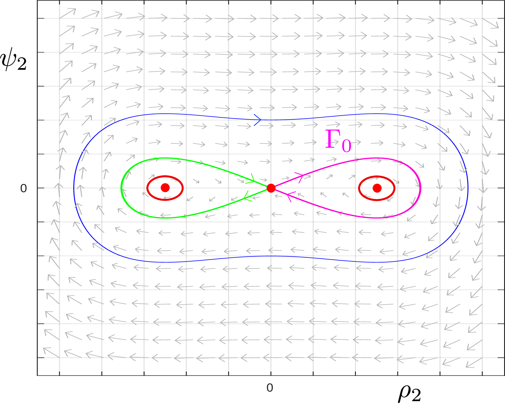
Figure 3: Phase portrait of (50 ) for \(b>0\)..
To follow Lazutkin’s approach one zooms in around the pole at \(t=-i\frac{\pi}{2}\) (the pole at \(t=i\frac{\pi}{2}\) is obtained by conjugation) by writing \[t=t(s):=-i\frac{\pi}{2}+r_2 s,\] and look for invariant manifolds parameterized by \(s\) and \(\theta\) as \(r_2\to 0\). For \(s\ne 0\), we have that \[\begin{align} \begin{cases} \rho_2(t(s)) =i\sqrt{\frac{2}{b}}\operatorname{csch}(r_2 s)= i\sqrt{\frac{2}{b}} (r_2s)^{-1}(1+ O(r_2^2)),\\ \psi_2(t(s)) =-i\sqrt{\frac{2}{b}} \operatorname{csch}(r_2 s)\operatorname{coth}(r_2 s) = -i\sqrt{\frac{2}{b}} (r_2s)^{-2}(1+ O(r_2^2)) \end{cases} \end{align}\] as \(r_2\to 0\) for \(s\ne 0\), or in terms of \((\rho,\psi)\) by (48 ): \[\begin{align} \label{eq:t2} \begin{cases} \rho(t(s)): = r_2 \rho_2(t(s)) \to i\sqrt{\frac{2}{b}} s^{-1},\\ \psi(t(s)):=r_2^2 \psi_2(t(s)) \to -i\sqrt{\frac{2}{b}} s^{-2}. \end{cases} \end{align}\tag{51}\] We then conclude that \[\begin{align} \psi = i\sqrt{\frac{b}{2}}\rho^2,\quad \psi\in \mathbb{C},\quad L=0,\quad \epsilon=0,\label{eq:this0} \end{align}\tag{52}\] defines an invariant set of (46 ). This can also easily be verified by direct insertion.
This motivates the definition of the inner problem associated with \(\Gamma_0\) as the unperturbed version of (45 ) (i.e. for \(\epsilon=0\)). In particular, we are concerned with invariant manifold solutions of the graph form \[\begin{align} \begin{cases} \psi= \psi(\rho,\theta),\\ L=L(\rho,\theta),\end{cases} \quad \rho\in B_\tau,\,\theta\in \mathbb{T}_\xi, \end{align}\] with \[\begin{align} \begin{cases} \psi(\rho,\theta)=i \sqrt{\frac{b}{2}}\rho^2(1+\mathcal{O}(\rho)),\\ L(\rho,\theta)=\mathcal{O}(\rho^4). \end{cases} \end{align}\] These manifolds are naturally parameterized in the \((r_1,\psi_1,L_1,\epsilon_1)\)-coordinates of the \(\breve \psi = 1\)-chart associated with the blowup (47 ): \[\begin{align} \label{eq:entry1hopfhopf} \begin{cases} \rho = r_1\\ \psi = r_1^2\psi_1,\\ L = r_1^3 L_1,\\ \epsilon =r_1^2\epsilon_1. \end{cases} \end{align}\tag{53}\] Indeed, here (52 ) takes the following form \[\begin{align} \psi_1 =i\sqrt{\frac{b}{2}},\quad r_1\in \mathbb{C},\quad L_1=0,\quad \epsilon_1=0.\label{eq:this2} \end{align}\tag{54}\] The change of coordinates defined by (53 ) brings (45 ) with \(\epsilon=0\) into the following form: \[\label{eq:innerhopfhopf} \begin{align} \dot{r}_1 &=r_1^2 \left(\psi_1+r_1^2U_1\right),\\ \dot{\psi}_1 &=r_1 (-b-2\psi_1^2+L_1^2)+r_1^2 Z_1,\\ \dot{L}_1 &=-3r_1 \psi_1 L_1+r_1^2 W_1,\\ \dot{\theta} &=1+r_1 L_1 +r_1^2 \beta+ r_1^3 V_1, \end{align}\tag{55}\] within \(\epsilon_1=0\). Here the functions \(Q_1=Q_1(\rho_1,r_1,L_1,\theta)\), \(Q=U,V,Z,W\), are analytic on \(B_\tau^3 \times \mathbb{T}_\xi\) with \(\tau>0\), \(\xi>0\) both small enough. They can obviously be expressed in terms of \(F,G,H,J\) but the details of this will not be important here. For (55 ), we look for invariant manifolds of the graph form \[\begin{align} \label{eq:this} \begin{cases} \psi_1=\Phi^{\psi}(r_1,\theta), \\ L_1=\Phi^L(r_1,\theta),\end{cases} \end{align}\tag{56}\] with \[\begin{align} \begin{cases} \Phi^\psi(0,\theta) =i\sqrt{\frac{b}{2}},\\ \Phi^L(0,\theta)=0.\end{cases} \end{align}\] The system (55 ) is reversible with respect to \[\begin{align} \label{eq:symmery1hopfhopf} \mathcal{S}_1\,:\,(r_1,\psi_1,L_1,\theta)\mapsto(r_1,-\psi_1,L_1,-\theta), \end{align}\tag{57}\] derived from (43 ), (44 ) and (53 ). Hence (56 ) is an invariant manifold solution if and only if \[\begin{align} \begin{cases} \psi_1=-\Phi^{\psi}(r_1,-\theta), \\ L_1=\Phi^L(r_1,-\theta),\end{cases} \end{align}\] is an invariant manifold solution.
3.1 Normal form↩︎
In this section, we show that (55 ) can be brought into the general form (3 ). We proceed as in Section 2.1 and first prove existence of formal series solutions. For this we use the following result from [32]: There exists a formal change of coordinates: \[\begin{align} \label{eq:Tinftyhopfhopf} (\widetilde{x},\widetilde{y},\widetilde{z},\widetilde{w}) = ( x, y, z, w) + T ( x, y, z, w), \end{align}\tag{58}\] with \(T\in \mathbb{R}[[( x, y, z, w)]]\) starting with terms of order \(5\), which brings (41 ) with \(\epsilon=0\) into the following formal normal form: \[\label{eq:nfhopfhopfformal} \begin{align} \dot{\widetilde{x}} &=-(1+\widetilde{\Omega})\widetilde{y}+\widetilde{z},\\ \dot{\widetilde{y}} &=(1+\widetilde{\Omega})\widetilde{x}+\widetilde{w},\\ \dot{\widetilde{z}} &= -(1+\widetilde{\Omega})\widetilde{w}+\widetilde{\Gamma} \widetilde{x}, \\ \dot{\widetilde{w}} &=(1+\widetilde{\Omega} )\widetilde{z}+\widetilde{\Gamma} \widetilde{y}, \end{align}\tag{59}\] where \[\begin{align} \widetilde{Q} \in \mathbb{R}[[\widetilde{\rho}^2,\widetilde{L}]],\quad \widetilde{Q}(0,0) = 0,\quad Q=\Omega,\Gamma, \end{align}\] with \[\begin{align} \widetilde{\rho}^2 = \widetilde{x}^2 + \widetilde{y}^2,\quad \widetilde{L} = \widetilde{w}\widetilde{x}-\widetilde{z}\widetilde{y}. \end{align}\] The formel change of coordinates defined by (58 ) is equivariant with respect to \(\mathcal{S}\). We have \[\begin{align} \label{eq:Gamma1} \widetilde{\Gamma}(\widetilde{\rho}^2,0)=- b \widetilde{\rho}^2 +\widetilde{\rho}^4 \widetilde{\Gamma}_1(\widetilde{\rho}^2),\quad \widetilde{\Gamma}_1\in \mathbb{R}[[\widetilde{\rho}^2]]. \end{align}\tag{60}\] We consider the change of coordinates \((\widetilde{\rho},\widetilde{\psi},\widetilde{L},\widetilde{\theta})\mapsto (\widetilde{x},\widetilde{y},\widetilde{z},\widetilde{w})\) defined by (44 ) (with tildes added), which brings (59 ) into the following system \[\nonumber \begin{align} \dot{\widetilde{\rho}} &=\widetilde{\psi},\\ \dot{\widetilde{\psi}} &= \widetilde{\Gamma} (\widetilde{\rho}^2,\widetilde{L})\widetilde{\rho} + \widetilde{\rho}^{-3} \widetilde{L}^2,\\ \dot{\widetilde{L}} &=0, \end{align}\] and \(\dot{\widetilde{\theta}} =1+\widetilde{\Omega} + \widetilde{\rho}^{-2} \widetilde{L}\), which decouples. This follows from a simple calculation. In particular, within \(\widetilde{L}=0\) we have \[\nonumber \begin{align} \dot{\widetilde{\rho}} &=\widetilde{\psi},\\ \dot{\widetilde{\psi}} &= \widetilde{\Gamma}(\widetilde{\rho}^2,0)\widetilde{\rho}, \end{align}\] with a nilpotent singularity at the origin (cf. (60 )). We therefore apply the directional blowup: \[\begin{align} \label{eq:directionalformel} (\widetilde{r}_1,\widetilde{\psi}_1)\mapsto \begin{cases} \widetilde{\rho} = \widetilde{r}_1,\\ \widetilde{\psi} = \widetilde{r}_1^2 \widetilde{\psi}_1, \end{cases} \end{align}\tag{61}\] in line with (53 ). This gives \[\label{eq:formelhopfhopf} \begin{align} (\widetilde{r}_1^2)' &=2\widetilde{r}_1^2\widetilde{\psi}_1,\\ \widetilde{\psi}_1' &=-b-2\widetilde{\psi}_1^2 + \widetilde{r}_1^2 \widetilde{\Gamma}_1(\widetilde{r}_1^2), \end{align}\tag{62}\] after division of the right hand side by \(\widetilde{r}_1\) (desingularization). Here we have used (60 ). Suppose first that \(b<0\). Then \((\widetilde{r}_1^2,\widetilde{\psi}_1)=(0,\pm \sqrt{\frac{-b}{2}})\) are (formal) hyperbolic singularities and we have formal stable respectively unstable manifolds of the form: \[\begin{align} \widetilde{\psi}_1 = \pm \widetilde{\Psi}(\widetilde{r}_1^2),\quad \widetilde{\Psi}\in \mathbb{R}[[\widetilde{r}_1^2]], \quad \widetilde{\Psi}(0)=\sqrt{\frac{-b}{2}}. \end{align}\] To see that the same is true for \(b>0\), we replace \((\widetilde{r}_1,\widetilde{\psi}_1)\) by \(i(\widetilde{r}_1,\widetilde{\psi}_1)\). This gives the following (real) system after multiplication of the right hand side by \(i\): \[\begin{align} (\widetilde{r}_1^2)' &=-\widetilde{r}_1^2\widetilde{\psi}_1,\\ \widetilde{\psi}_1' &=-b+2\widetilde{\psi}_1^2 - \widetilde{r}_1^2 \widetilde{\Gamma}_1(-\widetilde{r}_1^2). \end{align}\] Here \((\widetilde{r}_1^2,\widetilde{\psi}_1)=(0,\pm \sqrt{\frac{b}{2}})\) are (formal) hyperbolic singularities and we therefore obtain the same conclusion as for \(b<0\). We note that the two solutions (corresponding to \(\pm\)) are related by the symmetry \(\mathcal{S}_1\).
Lemma 3. Suppose that \(b\in \mathbb{R}\setminus\{0\}\). Then there is a formal invariant manifold of (55 ) of the form \[\begin{align} \begin{cases} \psi_1 = \Phi^{\psi}(r_1,\theta),\\ L_1 = \Phi^L(r_1,\theta), \end{cases} \end{align}\] with \[\begin{align} \label{eq:Phihopfhopf} \begin{cases} \Phi^{\psi}(r_1,\theta) =\sum_{\alpha=0}^\infty \Phi^{\psi}_\alpha(\theta)r_1^\alpha \in \mathbb{C}\{\theta\}[[r_1]] ,\\ \Phi^{L}(r_1,\theta) =\sum_{\alpha=3}^\infty \Phi^{L}_\alpha(\theta)r_1^\alpha \in r_1^3 \mathbb{C}\{\theta\}[[r_1]], \end{cases} \end{align}\qquad{(10)}\] and \[\begin{align} \Phi^\psi(0,\theta) = i\sqrt{\frac{b}{2}}. \end{align}\]
Proof. We write the formal series solution \[\begin{align} \label{eq:formalmanhopfhopf}\begin{cases} \widetilde{\psi}_1= \widetilde{\Psi} (\widetilde{r}_1^2),\\ \widetilde{L}_1=0, \end{cases} \end{align}\tag{63}\] of (59 ) in the \((r_1,\psi_1,L_1,\theta)\)-coordinates. By combining (44 ), (53 ), and (58 ), we obtain the following equations for (63 ) in the \((r_1,\psi_1,L_1,\theta)\)-coordinates: \[\begin{align} \widetilde{r}_1\cos \widetilde{\theta} &= r_1\cos \theta+\mathcal{O}(r_1^5),\\ \widetilde{r}_1 \sin \widetilde{\theta} &= r_1 \sin \theta+\mathcal{O}(r_1^5),\\ \widetilde{r}_1^2\widetilde{\Psi} \cos \widetilde{\theta} &= r_1^2\psi_1 \cos \theta-r_1^2 L_1\sin \theta+\mathcal{O}(r_1^5),\\ \widetilde{r}_1^2\widetilde{\Psi} \sin \widetilde{\theta} &= r_1^2\psi_1 \sin \theta+r_1^2 L_1 \cos \theta+\mathcal{O}(r_1^5), \end{align}\] where all \(\mathcal{O}(r_1^5)\in r_1^5 \mathbb{R}\{\psi_1,L_1,\theta\}[[r_1]]\). From the first two equations, we directly have that \[\begin{align} \widetilde{r}_1 = r_1\left(1 + \mathcal{O}(r_1^4)\right), \end{align}\] with \(\mathcal{O}(r_1^4)\in r_1^4 \mathbb{R}\{\psi_1,L_1,\theta\}[[r_1]]\). Inserting this into the last two equations, we find that \[\begin{align} \widetilde{\Psi}(r_1^2 (1+\mathcal{O}(r_1^4)))\times ( \cos \theta +\mathcal{O}(r_1^4)) &= \psi_1 \cos \theta-L_1\sin \theta+\mathcal{O}(r_1^3),\\ \widetilde{\Psi} (r_1^2 (1+\mathcal{O}(r_1^4)))\times ( \sin \theta +\mathcal{O}(r_1^4)) &= \psi_1 \sin \theta+L_1\cos \theta+\mathcal{O}(r_1^3). \end{align}\] But then using \(\widetilde{\Psi}(0)= i\sqrt{\frac{b}{2}}\), we arrive at the following formal equations \[\begin{align} \begin{cases} \psi_1-i\sqrt{\frac{b}{2}} +\mathcal{O}(r_1^3)=0,\\ L_1+\mathcal{O}(r_1^3)=0. \end{cases} \end{align}\] This follows from a simple calculation. We then complete the proof by solving these equations for \((\psi_1,L_1)\) (as formal series in \(r_1\) with real-analytic \(\theta\)-dependent coefficient) using the formal version of the implicit function theorem. ◻
We are now finally ready to bring (55 ) into the general form (3 ). For this we define \(\Phi^{\psi,N}\) and \(\Phi^{L,N}\), \(N\in \mathbb{N}\), \(N\ge 3\), as the partial sums: \[\begin{align} \Phi^{q,N}(r_1,\theta):=\sum_{\alpha=0}^N \Phi_{\alpha}^q(\theta)r_1^\alpha,\quad q=\psi,L, \end{align}\] recall (?? ).
Lemma 4. Suppose that \(b\ne 0\). Then for \(M\in \mathbb{N}\) sufficiently large, \(M\gg 1\), the blowup transformation \((r_1,\widetilde{\psi}_1,\widetilde{L}_1,\theta)\mapsto (r_1,\psi_1,L_1,\theta)\) defined by \[\begin{align} \label{eq:blowuprho1hopfhopf} \begin{cases} \psi_1 = \Phi^{\psi,2M}(r_1,\theta)+r_1^M \widetilde{\psi}_1,\\ L_1 = \Phi^{L,2M}(r_1,\theta)+r_1^M \widetilde{L}_1, \end{cases} \end{align}\qquad{(11)}\] brings (55 ) into the following prepared analytic form: \[\label{eq:nfhopfhopffinal} \begin{align} r_1'&=r_1^2 i\sqrt{\frac{b}{2}}+r_1^3 F_0 + r_1^4 Q(r_1,\widetilde{\psi}_1,\widetilde{L}_1,\theta),\\ \widetilde{\psi}_1'&= i\sqrt{\frac{b}{2}}r_1 \lambda^1 \widetilde{\psi}_1 +r_1^2 Z(r_1,\widetilde{\psi}_1,\widetilde{L}_1,\theta)\\ \widetilde{L}_1'&= i\sqrt{\frac{b}{2}} r_1 \lambda^2 \widetilde{L}_1 +r_1^2 Z(r_1,\widetilde{\psi}_1,\widetilde{L}_1,\theta),\\ \theta' &=1, \end{align}\qquad{(12)}\] after division of the right hand side by a nonzero quantity for \((r_1,\widetilde{\psi}_1,\widetilde{L}_1,\theta)\in B_\tau^3 \times \mathbb{T}_\xi\). Here \(\tau>0,\xi>0\), both small enough. The system is reversible with respect to \(\mathcal{S}_1\) (see (57 )). Finally, the following holds \[\begin{align} \lambda^1=-4-M<0,\quad \lambda^2 = -3-M<0. \end{align}\]
Proof. Since \(\psi_1=\Phi^{\psi,N}(r_1,\theta)\), \(L_1=\Phi^{L,N}(r_1,\theta)\), defines a formal invariant manifold for \(N\to \infty\), it follows by construction that \[\begin{align} \widetilde{Z}^N(r_1,\theta):=&r_1^{-N-1}\bigg( r_1 (-b-2(\Psi^{\psi,N})^2+(\Psi^{L,N})^2)+r_1^2 Z_1 \\ &-\frac{\partial \Phi^N}{\partial r_1} r_1^2 \left(\psi_1+r_1^2U_1\right)- \frac{\partial \Phi^N}{\partial \theta} \left(1+r_1 L_1 +r_1^2 \beta+ r_1^3 V_1\right)\bigg),\\ \widetilde{W}^N(r_1,\theta):=&r_1^{-N-1}\bigg(-3r_1 \Psi^{\psi,N}\Psi^{L,N}+r_1^2 W_1 \\ &-\frac{\partial \Phi^N}{\partial r_1} r_1^2 \left(\psi_1+r_1^2U_1\right)- \frac{\partial \Phi^N}{\partial \theta} \left(1+r_1 L_1 +r_1^2 \beta+ r_1^3 V_1\right)\bigg), \end{align}\] are well-defined and analytic on \(B_\tau \times \mathbb{T}_\xi\) for any \(N\in \mathbb{N}\) for \(\tau>0\), \(\xi>0\), both small enough. Here \(Q_1=Q_1(r_1,\Phi^{\psi,N},\Phi^{L,N},\theta)\), \(Q_1=U,V,Z,W\), recall (31 ). (Notice, in particular that \((\widetilde{Z}^N,\widetilde{W}^N)=(0,0)\) if and only if \(\psi_1=\Phi^{\psi,N}(r_1,\theta)\), \(L_1=\Phi^{L,N}(r_1,\theta)\), is invariant.) Then by applying (?? ) (corresponding to \(N=2M\)) to (27 ), we find the following equations \[\begin{align} \dot{r}_1 &= r_1^2 \left(i\sqrt{\frac{b}{2}}+F^M(r_1,r_1^M \widetilde{\psi}_1,r_1^M \widetilde{L}_1,\theta)\right),\\ \dot{\widetilde{\psi}}_1 &= r_1 A^M(r_1,r_1^M \widetilde{\psi}_1,r_1^M \widetilde{L}_1,\theta) \widetilde{\psi}_1+r_1 B^M(r_1,r_1^M \widetilde{\psi}_1,r_1^M \widetilde{L}_1,\theta) \widetilde{L}_1 + r_1^{M+1} \widetilde{Z}^{2M}(r_1,\theta),\\ \dot{\widetilde{L}}_1 &= r_1 C^M(r_1,r_1^M \widetilde{\psi}_1,r_1^M \widetilde{L}_1,\theta) \widetilde{\psi}_1+r_1 D^M(r_1,r_1^M \widetilde{\psi}_1,r_1^M \widetilde{L}_1,\theta) \widetilde{L}_1 + r_1^{M+1} \widetilde{W}^{2M}(r_1,\theta),\\ \dot{\theta} &=1+r_1 \Theta^M(r_1, r_1^M \widetilde{\psi}_1,r_1^M\widetilde{L}_1,\theta), \end{align}\] with \(F^M(0,0,0,\theta)=0\), \(\Theta^M(0,0,0,\theta)=0\), and \[\begin{align} \begin{cases} A^M(0,0,0,\theta)= -(4+M)i\sqrt{\frac{b}{2}},\\ B^M(0,0,0,\theta)=0,\\ C^M(0,0,0,\theta)=0,\\ D^M(0,0,0,\theta)= -(3+M)i\sqrt{\frac{b}{2}}, \end{cases} \end{align}\] This follows from a simple calculation using the mean-value theorem. We now divide the right hand side by \[1+r_1\Theta^M(r_1,r_1^M\widetilde{\psi}_1,r_1^M \widetilde{L}_1,\theta),\] which is nonzero on \(B_\tau^3 \times \mathbb{T}_\xi\) for \(\tau>0\), \(\xi>0\), both small enough. The result then follows from a simple expansion of the right hand side. (In fact, it is easy to see that \(M=2\) suffices.) ◻
We see that \[\begin{align} \label{eq:xhopfhopf} x:=i\sqrt{\frac{b}{2}}r_1,\quad \mathbf{y}: = (\widetilde{\psi}_1,\widetilde{L}_1), \end{align}\tag{64}\] brings (?? ) into the general form (3 ). Recall that \(\upsilon S^\pm\), \(\upsilon\in \mathbb{C}\), denotes the sets \[\begin{align} \upsilon S^\pm : =\{x\in \mathbb{C}\,:\,\upsilon^{-1}x\in S^\pm\}, \end{align}\] with \(S^\pm\) given by (?? ).
Proposition 10. Suppose that \(b\in \mathbb{R}\setminus\{0\}\) and define \[\begin{align} \upsilon:=i^{-1}\sqrt{\frac{2}{b}}. \end{align}\] Then for \(\delta>0\), \(\xi>0\), both sufficiently small, there exists two invariant manifold solutions of (55 ) of the form: \[\begin{align} \label{eq:invhopfhopf} \begin{cases} \psi_1 = \Phi^{\psi,\pm}(r_1,\theta),\\ L_1 = \Phi^{L,\pm}(r_1,\theta), \end{cases}\quad r_1\in \upsilon S^\pm,\,\theta\in \mathbb{T}_\xi, \end{align}\qquad{(13)}\] where \(\Phi^{\psi,\pm}(0,\theta)=i\sqrt{\frac{b}{2}}\), \(\Phi^{L,\pm}(r_1,\theta)=\mathcal{O}(r_1^4)\), uniformly on the closure of \(\upsilon S_\pm\), are the \(1\)-sums of Gevrey-\(1\) series in the directions defined by \(r_1\in \upsilon S^\pm\).
Proof. We first apply Theorem 1 to (?? ). This gives invariant manifolds of the form \[\begin{align} \begin{cases} \widetilde{\psi}_1 = \widetilde{\Phi}^{\psi,\pm}(r_1,\theta),\\ \widetilde{L}_1 = \widetilde{\Phi}^{L,\pm}(r_1,\theta), \end{cases}\quad r_1\in \upsilon S^\pm,\,\theta\in \mathbb{T}_\xi, \end{align}\] Here we have used (64 ) and that \(b\ne 0\). We then obtain the desired manifold (?? ) by blowing back down using (?? ). ◻
By applying the symmetry \(\mathcal{S}\), recall (57 ), we obtain a separate invariant manifolds solution: \[\begin{align} \nonumber \begin{cases} \psi_1 = -\Phi^{\psi,\pm}(r_1,-\theta),\\ L_1 = \Phi^{L,\pm}(r_1,-\theta), \end{cases}\quad r_1\in \upsilon S^\pm,\,\theta\in \mathbb{T}_\xi. \end{align}\]
Finally, we emphasize that Proposition 5 follows from Proposition 10 upon blowing down using (53 ).
4 A Banach-convolution-algebra-approach to Borel-Laplace↩︎
In this section, we review the Banach-convolution-algebra-approach to Borel-Laplace by Bonckaert and De Maesschalck [5] and extend it so that it can be applied to the PDE (1 ) (depending on \(\theta\in \mathbb{T}_\xi\)). We start by defining the appropriate Banach spaces and state the relevant properties from [5] relating to the convolution algebra (see Lemma 5).
4.1 The Banach space \(\mathcal{G}_\eta\)↩︎
We first consider analytic functions \[\begin{align} \label{eq:widehatW} \widehat W:\Omega \to \mathbb{C}, \end{align}\tag{65}\] where \(\Omega= \Omega(\kappa,\varphi,\nu)\subset \mathbb{C}\) is the star-shaped region defined by \[\begin{align} \label{eq:Omega} \Omega = B_{\kappa}\cup S(\varphi,\nu),\quad 0<\nu<\pi. \end{align}\tag{66}\] see Fig. [fig:Omega]. Here \(B_\kappa\subset \mathbb{C}\), \(\kappa>0\), is the open ball of radius \(\kappa>0\) centered at the origin. Moreover, \(S(\varphi,\nu)\subset \mathbb{C}\) denotes the infinite sector of opening \(\nu\in (0,\pi)\) centered along the direction defined by \(\varphi\in \mathbb{T}\); notice that \(S^\pm\) in (?? ) in contrast is a local sector of radius \(\delta\) (in the \(x\)-space). The argument of (65 ) is denoted by \(w\in \mathbb{C}\) and we refer to the \(w\)-space as the Borel-plane. Functions in the Borel-plane (like (65 )) are in this paper given a hat.
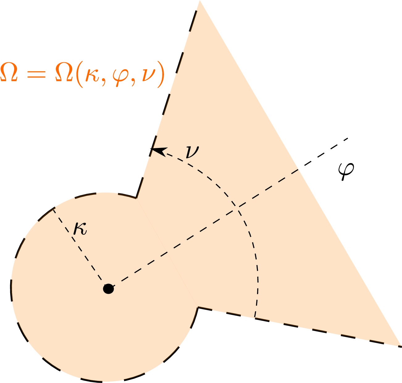
Figure 4: Illustration of the set \(\Omega\subset \mathbb{C}\). Here \(\varphi\in \mathbb{T}=\mathbb{R}/(2\pi\mathbb{Z})\) defines the direction of the sector, while \(\nu>0\) the opening. It will suffice for our purposes to take \(\varphi\in \{0,\pi\}\). Finally, \(\kappa>0\) is the radius of the disc..
It will suffice for our purposes to take \[\begin{align} \label{eq:thetacond} \varphi \in \{0,\pi\}; \end{align}\tag{67}\] \(S(\varphi,\nu)\) will therefore be centered along the positive real axis (corresponding to \(\varphi=0\)) or the negative real axis (corresponding to \(\varphi=\pi)\)), similar to the local sectors \(S^\pm\) in (?? ).
Following [5], we define \(\mathcal{G}_\eta\) for any \(\eta>0\) as the space of analytic functions (65 ) with \[\begin{align} \Vert \widehat W\Vert_{\eta}:=\sup_{w \in \Omega}\bigg\{\vert \widehat W(w)\vert {\mathrm e}^{-\eta \vert w\vert}(1+ \eta^2 \vert w\vert^2)\bigg\}<\infty. \end{align}\] \(\mathcal{G}_\eta\) with the norm \(\Vert \cdot\Vert_\eta\) is a Banach space for all \(\eta>0\). Since \[\begin{align} \label{eq:prop} {\mathrm e}^{-p}(1+p^2), \end{align}\tag{68}\] is a decreasing function of \(p\ge 0\), we have that \(\mathcal{G}_{\eta'}\subset \mathcal{G}_{\eta}\) for all \(\eta'>\eta\), see [5]. This property of (68 ) also implies that the constant function \(1\) has unit norm: \[\begin{align} \label{eq:unit} \Vert 1\Vert_\eta = 1, \end{align}\tag{69}\] for all \(\eta>0\). The factor \({\mathrm e}^{-\eta\vert w\vert }\) in the norm \(\Vert \cdot\Vert_\eta\) means that functions in \(\mathcal{G}_\eta\) can be Laplace transformed (see Lemma 7 below). On the other hand, the factor \((1+ \eta^2 \vert w\vert^2)\) ensures that the convolution product: \[\begin{align} \label{eq:convolution0} (\widehat W\star \widehat Z)(w) := w \int_0^1 \widehat W(ws) \widehat Z(w(1-s))ds,\quad \widehat W,\widehat Z:\Omega\to \mathbb{C}, \end{align}\tag{70}\] defines a bounded bilinear operator with a “small” operator norm (with respect to \(\eta\to \infty\)).
Lemma 5. [5] The following holds \[\begin{align} \Vert (\widehat W\star \widehat Z)\Vert_\eta \le 4\pi \eta^{-1} \Vert \widehat W\Vert_\eta \Vert \widehat Z\Vert_\eta, \end{align}\] for all \(\widehat W,\widehat Z\in \mathcal{G}_\eta\) and all \(\eta>0\).
Proof. It will be useful for us to repeat the proof from [5] (we will use it in the proof of Lemma 6 below): By the definition (70 ), we have the following estimate: \[\begin{align} \vert (\widehat W\star \widehat Z)(w)\vert&\le {\mathrm e}^{\eta \vert w\vert} (1+\eta^2 \vert w\vert^2)^{-1} \Vert \widehat W\Vert_\eta \Vert \widehat Z\Vert_\eta \int_0^{1} \frac{(1+\eta^2 \vert w\vert^2)}{(1+\eta^2 \vert w\vert^2 s^2)(1+\eta^2 \vert w\vert^2 (1-s)^2} \vert w\vert ds\\ &\le 8{\mathrm e}^{\eta \vert w\vert} (1+\eta^2 \vert w\vert^2)^{-1} \vert w\vert \Vert \widehat W\Vert_\eta \Vert \widehat Z\Vert_\eta\Vert \int_0^{\frac{1}{2}} \frac{\vert w\vert s}{1+\eta^2 \vert w\vert^4 s^4}\vert w \vert ds, \end{align}\] using the symmetry with respect to \(s\mapsto 1-s\) and that \(1+\eta^2 \vert w\vert^2 (1-s)^2\ge \frac{1}{4}(1+\eta^2 \vert w\vert^2)\) for all \(0\le s\le \frac{1}{2}\). We now apply the substitution \(p=\eta\vert w\vert s\): \[\begin{align} \int_0^{\frac{1}{2}} \frac{1}{1+\eta^2 \vert w\vert^2 s^2}\vert w \vert ds\le \eta^{-1} \int_0^{\infty} \frac{1}{1+s^2}ds = \frac{\pi}{2}\eta^{-1}, \end{align}\] so that \[\begin{align} \Vert (\widehat W\star \widehat Z)\Vert_{\eta} \le 4 \pi \eta^{-1} \Vert \widehat W\Vert_\eta \Vert \widehat Z\Vert_\eta. \end{align}\] ◻
In the present paper, we will also need the following result.
Lemma 6. Let \(\widehat W,\widehat Z\in \mathcal{G}_\eta\) and denote the function \[w\mapsto w \widehat W(w), \quad w\in \Omega,\] by \[w.\widehat{ W}.\] Then \[\begin{align} w\mapsto w^{-1} ((w.\widehat W)\star Z)(w), \quad w\in \Omega, \end{align}\] belongs to \(\mathcal{G}_\eta\), with the following uniform bound \[\begin{align} \Vert w\mapsto w^{-1} ((w.\widehat W)\star Z)(w) \Vert_\eta \le 4 \pi \eta^{-1} \Vert \widehat W \Vert_\eta \Vert \widehat Z \Vert_\eta,\quad \forall\,\eta>0, \end{align}\]
Proof. The proof is similar to Lemma 5. Indeed we have \[\begin{align} &\vert (w.\widehat W\star \widehat Z)(w)\vert\\ &\le {\mathrm e}^{\eta \vert w\vert} (1+\eta^2 \vert w\vert^2)^{-1}\Vert \widehat W\Vert_\eta \Vert \widehat Z\Vert_\eta \int_0^{1} \frac{ \vert w\vert s (1+\eta^2 \vert w\vert^2) }{(1+\eta^2 \vert w\vert^2 s^2)(1+\eta^2 \vert w\vert^2 (1-s)^2} \vert w\vert ds\\ &\le \vert w\vert \left( {\mathrm e}^{\eta \vert w\vert} (1+\eta^2 \vert w\vert^2)^{-1}\Vert \widehat W\Vert_\eta \Vert \widehat Z\Vert_\eta \int_0^{1} \frac{ 1+\eta^2 \vert w\vert^2 }{(1+\eta^2 \vert w\vert^2 s^2)(1+\eta^2 \vert w\vert^2 (1-s)^2} \vert w\vert ds\right), \end{align}\] using \(s\le 1\) in the final inequality. The last bracket is estimated above: \[\begin{align} \vert w^{-1} (w.\widehat W\star \widehat Z)(w)\vert {\mathrm e}^{-\eta \vert w\vert} (1+\eta^2 \vert w\vert^2)\le 4 \pi \eta^{-1} \Vert \widehat W\Vert_\eta \Vert \widehat Z\Vert_\eta, \end{align}\] for all \(w\in \Omega\), \(\eta>0\). ◻
4.2 The Laplace transform↩︎
Functions \(\widehat W\in \mathcal{G}_\eta\) can be Laplace transformed: \[\begin{align} \mathcal{L}^{\varphi}[\widehat W](x) = \int_0^{\infty{\mathrm e}^{i\varphi}} \widehat W(w) {\mathrm e}^{-w/x}dw, \end{align}\] where the integration is along the ray defined by \(w=r{\mathrm e}^{i\varphi}\), \(r\ge 0\). In particular, we have the following result:
Lemma 7. [5] The Laplace transform \(\mathcal{L}^{\varphi}\) defines (by analytic continuation) a linear continuous operator from \(\mathcal{G}_\eta\) to the set of analytic bounded functions on a sector \(S(\varphi,\pi + \nu)\cap B_\kappa\) (equipped with the sup-norm) where \[\begin{align} \kappa<\frac{1}{2} \eta^{-1} \sin \frac{\nu}{2}.\label{eq:deltacond} \end{align}\qquad{(14)}\] In particular, when (?? ) holds then we have the following bound: \[\begin{align} \label{eq:Laplacebound} \vert \mathcal{L}^{\varphi}[\widehat W](x) \vert\le \eta^{-1} \Vert \widehat W \Vert_\eta\quad \forall\,\widehat W\in \mathcal{G}_\eta, \end{align}\qquad{(15)}\] for all \(x\in S(\varphi,\pi + \nu)\cap B_\kappa\).
Proof. We refer to [5] for the proof. For comparison, we emphasize that we denote their \((\mu,\epsilon/2,\nu)\) by \((\eta,\nu,\delta)\) in the present manuscript. The bound (?? ) follows from the last estimate of the proof of [5] using (?? ). ◻
We recall that \[\begin{align} \label{eq:laplacewn} \mathcal{L}^{\varphi}\left[w\mapsto w^{\beta-1}\right](x)=(\beta-1)! x^\beta\quad \forall\,\beta\in \mathbb{N},\,\varphi\in \mathbb{T}. \end{align}\tag{71}\]
Remark 11. There is a different perspective of Borel-Laplace (resurgence [2]). Indeed, one could start from a Gevrey-1 series: \[\begin{align} \label{eq:series} W(x) = \sum_{\beta\in \mathbb{N}} W_\beta x^\beta,\quad \vert W_\beta\vert\le A \tau^\beta (\beta-1)! \end{align}\qquad{(16)}\] Then the Borel transform is given by \[\begin{align} \widehat W(w):=\sum_{\beta\in \mathbb{N}} W_{\beta} \frac{w^{\beta-1}}{(\beta-1)!}, \end{align}\] which is now convergent on the disc \(\vert w\vert<\tau^{-1}\). Then the series (?? ) is said to be \(1\)-summable in the direction \(\varphi\) if (a) the analytic function \(\widehat W\) can be endlessly continued to \(\widehat W^\varphi\) along the ray defined by \(w=r{\mathrm e}^{i\varphi}\), \(r\ge 0\), and (b) it is of at most exponential growth of order \(1\) along this ray, i.e. \[\begin{align} {\mathrm e}^{-\eta \vert w\vert} \vert \widehat W^\varphi(w)\vert =\mathcal{O}(1) \quad for\quad w\to \infty{\mathrm e}^{i\varphi}, \end{align}\] for some \(\eta>0\) large enough, see [1], [36]. Therefore, when the series is \(1\)-summable, then the extension \(\widehat W^\varphi\) of \(\widehat W\) can be Laplace-transformed \(\mathcal{L}^{\varphi}[\widehat W^\varphi]\) to obtain an analytic function \(W^\varphi\) of \(x\) in some local sector (like \(S^\pm\) in (?? )), see Lemma 7.
In this paper, our viewpoint is slightly different. Instead of trying to establish the Gevrey-property of the asymptotic series first and then perform the continuation of the Borel transform, we achieve this more indirectly by following [5]. The idea is to set up an appropriate nonlinear equation in \(\mathcal{G}_\eta\) for the Borel transform \(\widehat W=\widehat W^\varphi\) of our unknown function. Importantly, this equation in the Borel plane is perturbative by Lemma 5 for \(\eta\gg 1\) and it can therefore (easily!) be solved by a fixed-point argument. Finally, the desired solution is obtained through the Laplace transform (which is well-defined by Lemma 7). In this way, we also obtain the Gevrey-\(1\) asymptotic series in a more indirect way: We can write \(\widehat W\) as a convergent series \(\widehat W(w) = \sum_{\beta\in \mathbb{N}} \widehat W_\beta w^{\beta-1}\), \(\vert W_\beta\vert\le A \tau^\beta\), \(A>0,\tau>0\), near the origin (this is the motivation for including the open ball \(B_\kappa\) in \(\Omega\), see (66 )). We then obtain the Gevrey-\(1\) asymptotic series by applying the formal Laplace transformation (recall (71 )): \[\begin{align} W(x) \sim_1 \sum_{\alpha \in \mathbb{N}} \widehat W_\beta(\beta-1)! x^\beta,\quad x\in S(\varphi,\pi+\nu)\cap B_\kappa. \end{align}\]
To transform the equation (1 ) into an equation in the Borel plane for the Borel-transform \(\widehat{\mathbf{y}}\) of \(\mathbf{y}\), we will use the following basic properties of the Laplace transform: \[\begin{align} \mathcal{L}^{\varphi}[\widehat W\star \widehat Z] =\mathcal{L}^{\varphi}[\widehat W]\mathcal{L}^{\varphi}[\widehat Z],\label{eq:prop1} \end{align}\qquad{(17)}\] and \[\begin{align} x^2 \frac{d}{dx} \mathcal{L}^{\varphi}[\widehat W](x) = \mathcal{L}^{\varphi}[w.\widehat W](x).\label{eq:prop2} \end{align}\qquad{(18)}\] together with Lemma 10. See Section 5 for further details.
In the following section, we consider Fourier series with coefficients in \(\mathcal{G}_\eta\).
4.3 The Banach space \(\mathcal{G}_\eta\{{\mathrm e}^{i\theta}\}\)↩︎
Next, we consider analytic functions: \[\begin{align} \label{eq:mathcalWtheta} \widehat W\,:\,\Omega \times \mathbb{T}_\xi \to \mathbb{C},\quad \mathbb{T}_\xi := \mathbb{C}/(2\pi \mathbb{Z}), \end{align}\tag{72}\] which we write as Fourier series: \[\begin{align} \widehat W (w,\theta ) = \sum_{\alpha\in \mathbb{Z}}\widehat W_\alpha(w) {\mathrm e}^{i\alpha \theta}, \end{align}\] and suppose that \(\widehat W_\alpha\in \mathcal{G}_\eta\) for all \(\alpha\in \mathbb{Z}\). In particular, we define \(\mathcal{G}_\eta\{{\mathrm e}^{i\theta}\}\), \(\eta>0\), as the space of analytic functions (72 ) with \[\begin{align} \label{eq:Wert} {\vert\kern-0.25ex\vert\kern-0.25ex\vert}\widehat W{\vert\kern-0.25ex\vert\kern-0.25ex\vert}_{\eta}:= \sup_{\theta \in \mathbb{T}_\xi} \left\{\sum_{\alpha\in \mathbb{Z}} \Vert \widehat W_\alpha\Vert_{\eta} {\mathrm e}^{-\alpha \operatorname{Im}\theta}\right\}<\infty. \end{align}\tag{73}\] \(\mathcal{G}_\eta\{{\mathrm e}^{i\theta}\}\) with the norm \({\vert\kern-0.25ex\vert\kern-0.25ex\vert}\cdot{\vert\kern-0.25ex\vert\kern-0.25ex\vert}_\eta\) is also a Banach space for all \(\eta>0\), with \(\mathcal{G}_{\eta'}\{{\mathrm e}^{i\theta}\}\subset \mathcal{G}_\eta\{{\mathrm e}^{i\theta}\}\) for all \(\eta'>\eta\).
Remark 12. Notice that \[\begin{align} \frac{1}{2} \sum_{\alpha\in \mathbb{Z}} \Vert \widehat W_\alpha\Vert_{\eta} {\mathrm e}^{\vert \alpha\vert \xi} \le {\vert\kern-0.25ex\vert\kern-0.25ex\vert}\widehat W{\vert\kern-0.25ex\vert\kern-0.25ex\vert}_{\eta}\le \sum_{\alpha\in \mathbb{Z}} \Vert \widehat W_\alpha\Vert_{\eta} {\mathrm e}^{\vert \alpha\vert \xi}. \end{align}\] The upper bound is obvious. For the lower bound, we set \(\operatorname{Im}\theta=\pm \xi\): \[\begin{align} \sum_{-\alpha\in \mathbb{N}} \Vert \widehat W_\alpha\Vert_{\eta} {\mathrm e}^{-\alpha \xi} \le \sum_{\alpha\in \mathbb{Z}} \Vert \widehat W_\alpha\Vert_{\eta} {\mathrm e}^{-\alpha \xi}\le {\vert\kern-0.25ex\vert\kern-0.25ex\vert}\widehat W{\vert\kern-0.25ex\vert\kern-0.25ex\vert}_{\eta},\\ \sum_{\alpha\in \mathbb{N}_0} \Vert \widehat W_\alpha\Vert_{\eta} {\mathrm e}^{\alpha \xi} \le \sum_{\alpha\in \mathbb{Z}} \Vert \widehat W_\alpha\Vert_{\eta} {\mathrm e}^{\alpha \xi}\le {\vert\kern-0.25ex\vert\kern-0.25ex\vert}\widehat W{\vert\kern-0.25ex\vert\kern-0.25ex\vert}_{\eta}, \end{align}\] proving that \[\begin{align} \sum_{\alpha\in \mathbb{Z}} \Vert \widehat W_\alpha\Vert_{\eta} {\mathrm e}^{\vert \alpha\vert \xi}\le 2{\vert\kern-0.25ex\vert\kern-0.25ex\vert}\widehat W{\vert\kern-0.25ex\vert\kern-0.25ex\vert}_{\eta} \end{align}\] It follows that \(\widehat W\in \mathcal{G}_\eta\{{\mathrm e}^{i\theta}\}\) implies that \[\begin{align} \Vert \widehat W_\alpha \Vert_{\eta}{\mathrm e}^{\vert \alpha\vert \xi}\to 0 \quad for \alpha\to \infty. \end{align}\] We prefer to work with the norm \({\vert\kern-0.25ex\vert\kern-0.25ex\vert}\widehat W{\vert\kern-0.25ex\vert\kern-0.25ex\vert}_\eta\) (rather than e.g. the equivalent norm \(\sum_{\alpha\in \mathbb{Z}} \Vert \widehat W_\alpha\Vert_{\eta} {\mathrm e}^{\vert \alpha\vert \xi}\)) as it performs well under multiplication (see Lemma 9).
We Laplace transform the functions (72 ) term-wise, i.e. \[\begin{align} \label{eq:laplacedefn} \mathcal{L}^{\varphi}[\widehat W][(x,\theta): = \sum_{\alpha\in\mathbb{Z}} \mathcal{L}^{\varphi} [\widehat W_\alpha](x) {\mathrm e}^{i\alpha \theta}. \end{align}\tag{74}\] We have the following:
Lemma 8. \(\mathcal{L}^{\varphi}\) is a bounded linear operator from \(\mathcal{G}_\eta\{{\mathrm e}^{i\theta}\}\) to the space of analytic defined on \((x,\theta)\in (S(\varphi,\pi+\nu)\cap B_\kappa)\times \mathbb{T}_\xi\) for \(\kappa>0\) small enough, see (?? ). In particular, whenever (?? ) holds then we have the following estimate: \[\begin{align} \vert \mathcal{L}^{\varphi}[\widehat W](x,\theta)\vert\le \eta^{-1} {\vert\kern-0.25ex\vert\kern-0.25ex\vert}W{\vert\kern-0.25ex\vert\kern-0.25ex\vert}_\eta, \end{align}\] for all \((x,\theta)\in (S(\varphi,\pi+\nu)\cap B_\kappa)\times \mathbb{T}_\xi\).
Proof. By Lemma 7, it suffices to show the bound. We find that \[\begin{align} \vert \mathcal{L}^{\varphi}[\widehat W](x,\theta)\vert &\le \eta^{-1} \sum_{\alpha\in\mathbb{Z}} \Vert \widehat W_\alpha\Vert_\eta {\mathrm e}^{-\alpha \operatorname{Im}(\theta)}\le \eta^{-1} {\vert\kern-0.25ex\vert\kern-0.25ex\vert}W{\vert\kern-0.25ex\vert\kern-0.25ex\vert}_\eta, \end{align}\] by (?? ) and (74 ). ◻
Now, the product of Fourier series is given by “convolution of the coefficients” (Cauchy’s product rule): \[\begin{align} \label{eq:cauchy} \sum_{\alpha \in \mathbb{Z}}f_\alpha{\mathrm e}^{i\alpha \theta}\sum_{\beta \in \mathbb{Z}}g_\beta{\mathrm e}^{i\beta\theta} = \sum_{\alpha\in \mathbb{Z}}\left(\sum_{\beta\in \mathbb{Z}} f_\beta g_{\alpha-\beta}\right){\mathrm e}^{i\alpha \theta}, \end{align}\tag{75}\] and we therefore define the convolution on \(\mathcal{G}_\eta\{{\mathrm e}^{i\theta}\}\) at the level of the coefficients in the following way: \[\begin{align} \label{eq:convolution2} (\widehat W\star \widehat Z)(w,\theta):=\sum_{\alpha\in \mathbb{Z}} \left(\sum_{\beta \in \mathbb{Z}} \widehat W_\beta \star \widehat Z_{\alpha-\beta}\right) {\mathrm e}^{i\alpha \theta}\quad \forall\,\widehat W,\,\widehat Z\in \mathcal{G}_\eta\{{\mathrm e}^{i\theta}\}. \end{align}\tag{76}\] In this way, \[\begin{align} \label{eq:laplacefs} \mathcal{L}^{\varphi}[\widehat W\star \widehat Z]= \mathcal{L}^{\varphi}[\widehat W]\mathcal{L}^{\varphi}[\widehat Z]\quad \forall\,\widehat W,\widehat Z\in \mathcal{G}_\eta\{{\mathrm e}^{i\theta}\}. \end{align}\tag{77}\]
Lemma 9. The convolution defines a bounded bilinear operator \(\mathcal{G}_\eta\{{\mathrm e}^{i\theta}\}\times \mathcal{G}_\eta\{{\mathrm e}^{i\theta}\}\to \mathcal{G}_\eta\{{\mathrm e}^{i\theta}\}\): \[\begin{align} {\vert\kern-0.25ex\vert\kern-0.25ex\vert}\widehat W\star \widehat Z{\vert\kern-0.25ex\vert\kern-0.25ex\vert}_\eta \le 4 \pi \eta^{-1}{\vert\kern-0.25ex\vert\kern-0.25ex\vert}\widehat W{\vert\kern-0.25ex\vert\kern-0.25ex\vert}_\eta {\vert\kern-0.25ex\vert\kern-0.25ex\vert}\widehat Z{\vert\kern-0.25ex\vert\kern-0.25ex\vert}_\eta, \end{align}\] for all \(\widehat W,\widehat Z\in \mathcal{G}_\eta\{{\mathrm e}^{i\theta}\}\) and any \(\eta>0\).
Proof. By definition (76 ), we have \(\widehat W\star \widehat Z=\sum_{\alpha\in \mathbb{Z}}(\widehat W\star \widehat Z)_\alpha {\mathrm e}^{i\theta}\) with \[\begin{align} (\widehat W\star \widehat Z)_\alpha(w)=\sum_{\beta\in \mathbb{Z}} w \int_0^1 \widehat W_{\beta}(ws) \widehat Z_{\alpha-\beta}(w(1-s)) ds. \end{align}\] From Lemma 5, we have \[\begin{align} \Vert (\widehat W\star \widehat Z)_\alpha\Vert_{\eta} \le 4 \pi \eta^{-1} \sum_{\beta\in \mathbb{Z}} \Vert \widehat W_\beta\Vert_\eta \Vert \widehat Z_{\alpha-\beta}\Vert. \end{align}\] This leads to the following estimate (upon using (75 )) for any \(\theta\in \mathbb{T}_\xi\) \[\begin{align} \sum_{\alpha\in \mathbb{Z}} \Vert (\widehat W\star \widehat Z)_\alpha \Vert_\eta {\mathrm e}^{-\alpha \operatorname{Im}\theta} &\le 4 \pi \eta^{-1} \sum_{\alpha\in \mathbb{Z}}\sum_{\beta\in \mathbb{Z}} \Vert W_\beta\Vert_\eta e^{-\beta \operatorname{Im}\theta} \Vert \widehat Z_{\alpha-\beta}\Vert e^{-(\alpha-\beta) \operatorname{Im}\theta} \\ &= 4 \pi \eta^{-1} \sum_{\alpha'\in \mathbb{Z}}\Vert \widehat W_{\alpha'}\Vert_\eta e^{-\alpha' \operatorname{Im}\theta} \sum_{\beta'\in \mathbb{Z}}\Vert \widehat Z_{\beta'} \Vert_\eta e^{-\beta' \operatorname{Im}\theta}\\ &\le4 \pi \eta^{-1} {\vert\kern-0.25ex\vert\kern-0.25ex\vert}\widehat W{\vert\kern-0.25ex\vert\kern-0.25ex\vert}_\eta {\vert\kern-0.25ex\vert\kern-0.25ex\vert}\widehat Z{\vert\kern-0.25ex\vert\kern-0.25ex\vert}_\eta. \end{align}\] Here we have taking the sup over \(\theta\in \mathbb{T}_{\xi}\) in the last inequality, recall (73 ). The result then follows. ◻
4.4 The Banach spaces \(\mathcal{G}^n_\eta\) and \(\mathcal{G}^n_\eta\{{\mathrm e}^{i\theta}\}\)↩︎
Finally, we define \(\mathcal{G}^n_{\eta}\) (\(\mathcal{G}^n_\eta\{{\mathrm e}^{i\theta}\}\)) as the space of analytic functions \(\widehat{\mathbf{W}}=(\widehat W^1,\ldots,\widehat W^n)\,:\Omega \to \mathbb{C}^n\) ( \(\widehat{\mathbf{W}}=(\widehat W^1,\ldots,\widehat W^n)\,:\Omega\times \mathbb{T}_\xi \to \mathbb{C}^n\)) with each component \(\widehat{W}^j\), \(j\in \{1,\ldots,n\}\), belonging to \(\mathcal{G}_\eta\) (\(\mathcal{G}_\eta\{{\mathrm e}^{i\theta}\}\), respectively). We then equip these spaces with the following Banach norms \[\begin{align} \Vert \widehat{\mathbf{W}}\Vert_\eta:=\sup_{j\in \{1,\ldots,n\}} \Vert \widehat W^j\Vert_\eta,\label{eq:Vertn} \end{align}\tag{78}\] and \[\begin{align} {\vert\kern-0.25ex\vert\kern-0.25ex\vert}\widehat{\mathbf{W}}{\vert\kern-0.25ex\vert\kern-0.25ex\vert}_\eta:=\sup_{j\in \{1,\ldots,n\}} {\vert\kern-0.25ex\vert\kern-0.25ex\vert}\widehat W^j{\vert\kern-0.25ex\vert\kern-0.25ex\vert}_\eta,\label{eq:Wertn} \end{align}\tag{79}\] respectively. We use bold to denote symbols in \(\mathbb{C}^n\) and therefore it should be clear from the context whether the norms are understood on \(\mathbb{C}\) (as on the right hand sides of (78 ) and (79 )) or on \(\mathbb{C}^n\) (as on the left hand sides of (78 ) and (79 )).
4.5 Further results↩︎
We will need a few additional results regarding \(\mathcal{G}^n_\eta\), \(n\ge 1\), from [5], that we list as follows.
Firstly, suppose that \(Q(x) = \sum_{\beta\in \mathbb{N}} Q_\beta x^\beta\) is a convergent series, \(\vert Q_\beta\vert \le A \tau^\beta\), \(A,\tau>0\). Then the Borel-transform of \(Q\): \[\begin{align} \widehat Q(w): = \sum_{\beta\in \mathbb{N}} Q_\beta \frac{w^{\beta-1}}{(\beta-1)!}, \end{align}\] is an entire function with at most exponential growth of order \(1\) for \(w\to \infty\): \[\begin{align} \vert \widehat Q(w)\vert \le A{\mathrm e}^{\tau w}\quad\forall\,w\in \mathbb{C}. \end{align}\] In particular, \(\Vert \widehat Q\Vert_\eta \le A\) for \(\eta>0\) large enough, see [5].
Next, we consider a convergent series \(Q(x,\mathbf{z})=\sum_{\beta\in \mathbb{N}^n} Q_\beta(x){ \mathbf{z}}^\beta\), \({\mathbf{z}}=(z^1,\ldots,z^n)\in B_\kappa^n\subset \mathbb{C}^n\), with \(Q_\beta(x)=\sum_{\gamma=1}^\infty Q_{\beta,\gamma} x^\gamma\), \(\vert Q_{\beta,\gamma}\vert\le A \tau^{\vert \beta\vert+\gamma}\), \(\vert \beta\vert = \beta^1+\cdots +\beta^n\), \(A>0,\tau>0\). Here \({ \mathbf{z}}^\beta = (z^1)^{\beta^1}\cdots (z^n)^{\beta^n}\) as usual. We then define \[\begin{align} \widehat Q(\widehat{\mathbf{z}}) :=\sum_{\beta\in \mathbb{N}^n} \widehat Q_\beta\star \widehat{\mathbf{z}}^{\star \beta}, \end{align}\] where \(\widehat Q_\beta(w) = \sum_{\gamma=1}^\infty Q_{\beta,\gamma} \frac{w^{\gamma-1}}{(\gamma-1)!}\) denotes the Borel transform of \(Q_\beta\). By item ([item10]), we have that \(\Vert \widehat Q_\beta\Vert_\eta\le A \tau^{\vert \beta\vert}\). Now, suppose that \(\widehat{\mathbf{z}}\in \mathcal{G}^n_\eta\) and that \(\Vert \widehat{\mathbf{z}}\Vert_\eta\le C_1\), for any fixed \(C_1>0\). Then there is a \(\eta_0(C_1)>0\) large enough such that \[\begin{align} \Vert \widehat Q(\widehat{\mathbf{z}})\Vert_\eta\le 2^n A\tau, \end{align}\] for all \(\eta>\eta_0\), see [5]. Moreover, \[\begin{align} \mathcal{L}[\widehat Q(\widehat{\mathbf{z}})](x) = Q(x,\mathcal{L}[\widehat{\mathbf{z}}](x)), \end{align}\] for all \(x\in S(\varphi,\pi + \nu)\cap B_\kappa\).
Finally, \(\widehat{\mathbf{z}}\mapsto \widehat Q(\widehat{\mathbf{z}})\), \(\Vert \widehat{\mathbf{z}}\Vert_\eta\le C_1\), \(\eta>\eta_0\), is \(C^1\), see [5], with \[\begin{align} D\widehat Q(\widehat{\mathbf{z}})(\widehat{\mathbf{w}}): = \sum_{i=1}^n \widehat{\left(\frac{\partial Q}{\partial z^j} \right)} \star \widehat w^j, \end{align}\] where \(\widehat{\mathbf{q}}=(\widehat q^1,\ldots,\widehat q^n)\), \(\mathbf{q}=\mathbf{z},\mathbf{w}\), with the following bound \[\begin{align} \Vert D\widehat Q(\widehat{\mathbf{z}})\Vert_\eta \le \mathcal{O}(\eta^{-1}), \end{align}\] for all \(\Vert \widehat{\mathbf{z}}\Vert_\eta\le C_1\).
Consider \(Q\) as in item ([this]). In the present paper, we then define \(\widehat Q(\widehat{\mathbf{z}})\) analogously for \(\widehat{\mathbf{z}}\in \mathcal{G}_\eta^n\{{\mathrm e}^{i\theta}\}\): \[\begin{align} \widehat Q(\widehat{\mathbf{z}}) :=\sum_{\beta\in \mathbb{N}^n} \widehat Q_\beta(w)\star \widehat{\mathbf{z}}^{\star \beta}.\label{eq:widehatFalpha} \end{align}\tag{80}\] We similarly have that \(\widehat Q(\widehat{\mathbf{z}}) \in \mathcal{G}_\eta\{{\mathrm e}^{i\theta}\}\) for all \({\vert\kern-0.25ex\vert\kern-0.25ex\vert}\widehat{\mathbf{z}}{\vert\kern-0.25ex\vert\kern-0.25ex\vert}_\eta\le C_1\) provided that \(\eta>\eta_0\). Indeed, by Lemma 9, we have that \[\begin{align} {\vert\kern-0.25ex\vert\kern-0.25ex\vert}\widehat Q(\widehat{\mathbf{z}}){\vert\kern-0.25ex\vert\kern-0.25ex\vert}_\eta&\le \sum_{\beta\in \mathbb{N}^n} \Vert \widehat Q_\beta\Vert_\eta \left(4\pi \eta^{-1} {\vert\kern-0.25ex\vert\kern-0.25ex\vert}\widehat{\mathbf{z}}{\vert\kern-0.25ex\vert\kern-0.25ex\vert}\right)^{\vert \beta\vert}\\ &\le A\sum_{\beta\in \mathbb{N}^n} \left(4\pi \eta^{-1} \tau {\vert\kern-0.25ex\vert\kern-0.25ex\vert}\widehat{\mathbf{z}}{\vert\kern-0.25ex\vert\kern-0.25ex\vert}\right)^{\vert \beta\vert}\\ &=A \left(\sum_{\vert \beta\vert=1}^\infty \left(4\pi \eta^{-1} \tau {\vert\kern-0.25ex\vert\kern-0.25ex\vert}\widehat{\mathbf{z}}{\vert\kern-0.25ex\vert\kern-0.25ex\vert}\right)^{\vert \beta\vert}\right)^n\\ &\le A (1-4\pi \eta^{-1}\tau C_1)^{-n}, \end{align}\] using that \({\vert\kern-0.25ex\vert\kern-0.25ex\vert}\widehat Q_\beta{\vert\kern-0.25ex\vert\kern-0.25ex\vert}_\eta = \Vert \widehat Q_\beta\Vert_\eta\le A\tau ^{\vert \beta\vert}\) since \(\widehat Q_\beta\) is independent of \(\theta\). For any \(\eta>8\pi \tau C_1\), we therefore have that \[\begin{align} {\vert\kern-0.25ex\vert\kern-0.25ex\vert}\widehat Q(\widehat{\mathbf{z}}){\vert\kern-0.25ex\vert\kern-0.25ex\vert}_\eta\le 2^{n} A. \end{align}\] We also have that \[\begin{align} \mathcal{L}^{\varphi}( \widehat Q(\widehat{\mathbf{z}}))(x,\theta) = Q(x,\mathcal{L}^{\varphi}(\widehat{\mathbf{z}})(x,\theta)), \end{align}\] for all \(x\in S(\varphi,\pi + \nu)\cap B_\kappa\), \(\theta\in \mathbb{T}_\xi\). This follows from Lemma 8 and (77 ).
We now finally turn to the Borel transform of analytic Fourier series \[\begin{align} Q(x,\mathbf{z},\theta) = \sum_{\alpha\in \mathbb{Z}} Q_{\alpha}(x,\mathbf{z}) {\mathrm e}^{i\alpha \theta}, \end{align}\] with \[\begin{align} \label{eq:cond1} Q_\alpha(x,\mathbf{z}) = \sum_{\beta \in \mathbb{N}^n} Q_{\alpha,\beta} (x) \mathbf{z}^\beta,\quad Q_{\alpha,\beta} (x) = \sum_{\gamma=1}^n Q_{\alpha,\beta,\gamma} x^\gamma. \end{align}\tag{81}\] In further details, we suppose that \(Q\) is analytic on \((x,\mathbf{z},\theta) \in B_\kappa \times B_\kappa^n \times \mathbb{T}_\zeta\) with \(\zeta>\xi\), \(\kappa>0\). We therefore suppose that \[\begin{align} \label{eq:cond2} \vert Q_{\alpha,\beta,\gamma}\vert \le A \tau^{\vert\beta\vert +\gamma} {\mathrm e}^{-\zeta \vert \alpha\vert}\quad \forall\,\alpha \in \mathbb{Z},\,\beta\in \mathbb{N}^n,\,\gamma\in \mathbb{N}, \end{align}\tag{82}\] with \(A>0\), \(\tau>0\) large enough, after possibly decreasing \(\zeta>0\) and \(\kappa>0\). We then define the Borel transform of \(Q\) as follows: \[\begin{align} \widehat Q(\widehat{\mathbf{z}})(w,\theta):=\sum_{\beta\in \mathbb{N}^n} \left(\sum_{\alpha\in \mathbb{Z}} \widehat Q_{\alpha,\beta}(w) {\mathrm e}^{i\alpha \theta}\right) \star \widehat{\mathbf{z}}^{\star \beta},\label{eq:widehatF} \end{align}\tag{83}\] where \(\widehat Q_{\alpha,\beta}\) is the Borel transform of \(Q_{\alpha,\beta}\): \[\begin{align} \widehat Q_{\alpha,\beta}(w):= \sum_{\gamma=1}^\infty Q_{\alpha,\beta,\gamma} \frac{w^{\gamma-1}}{(\gamma-1)!}.\label{eq:Qab} \end{align}\tag{84}\]
Lemma 10. Consider (83 ) and (84 ), satisfying (81 ) and (82 ). Then \[\begin{align} \widehat{Q}\,:\, B_{C_1}^{\mathcal{G}} \to \mathcal{G}_\eta \{{\mathrm e}^{i\theta}\}, \end{align}\] where \(B_{C_1}^{\mathcal{G}}\) is the open ball of radius \(C_1>0\) in \(\mathcal{G}^n_\eta\{{\mathrm e}^{i\theta}\}\), is well-defined and \(C^1\) for all \(\eta>\eta_0(C_1)>0\) with the following uniform bounds: \[\begin{align} \label{eq:Qbound} \begin{cases} \sup_{\widehat{\mathbf{z}}\in B_{C_1}^{\mathcal{G}}} {\vert\kern-0.25ex\vert\kern-0.25ex\vert}\widehat Q(\widehat{\mathbf{z}}){\vert\kern-0.25ex\vert\kern-0.25ex\vert}_\eta \le \frac{2^{n+1} A}{1-{\mathrm e}^{-(\zeta-\xi)}},\\ \sup_{\widehat{\mathbf{z}}\in B_{C_1}^{\mathcal{G}}}\Vert D\widehat Q(\widehat{\mathbf{z}})\Vert =\mathcal{O}(\eta^{-1}). \end{cases} \end{align}\qquad{(19)}\] Finally, \[\begin{align} \mathcal{L}^{\varphi}(\widehat{Q}(\widehat{\mathbf{z}}))(x,\theta)= Q(x,\mathcal{L}^{\varphi}(\widehat{\mathbf{z}})(x,\theta),\theta), \end{align}\] for all \((x,\theta)\in (S(\varphi,\theta+\nu)\cap B_\kappa)\times \mathbb{T}_\xi\) with \(\kappa>0\) small enough.
Proof. First, we notice that \[\begin{align} {\vert\kern-0.25ex\vert\kern-0.25ex\vert}\sum_{\alpha\in \mathbb{Z}} \widehat Q_{\alpha,\beta}(w) {\mathrm e}^{i\alpha \theta}{\vert\kern-0.25ex\vert\kern-0.25ex\vert}_\eta \le A \tau^{\vert\beta\vert} \sum_{\alpha \in\mathbb{Z}} {\mathrm e}^{-\vert \alpha\vert(\zeta-\xi)}\le\frac{ 2A \tau^{\vert \beta\vert} }{1-{\mathrm e}^{-(\zeta-\xi)}}, \end{align}\] recall item ([item10]) above. But then by Lemma 9, we find that \[\begin{align} {\vert\kern-0.25ex\vert\kern-0.25ex\vert}\widehat Q(\widehat{\mathbf{z}}){\vert\kern-0.25ex\vert\kern-0.25ex\vert}_\eta&\le\sum_{\beta\in \mathbb{N}^n} \frac{ 2A \tau^{\vert \beta\vert} }{1-{\mathrm e}^{-(\zeta-\xi)}} \left(4\pi \eta^{-1} {\vert\kern-0.25ex\vert\kern-0.25ex\vert}\widehat{\mathbf{z}}{\vert\kern-0.25ex\vert\kern-0.25ex\vert}_\eta\right)^{\vert \beta\vert}\\ &\le \frac{2^{n+1} A}{1-{\mathrm e}^{-(\zeta-\xi)}}, \end{align}\] for all \({\vert\kern-0.25ex\vert\kern-0.25ex\vert}\widehat{\mathbf{z}}{\vert\kern-0.25ex\vert\kern-0.25ex\vert}_\eta\le C_1\) provided that \(\eta>8\pi \tau C_1\). The fact that \(\widehat Q\) is \(C^1\) proceeds completely analagously, see also the text around [5]. ◻
5 Equations in the Borel plane↩︎
In this section, we now finally turn to solving (1 ), repeated here for convenience \[\begin{align} \label{eq:inveqn} x^2 \mathbf{y}'_x (1+xF_0+x^2 F_1)+\mathbf{y}'_\theta+x \mathbf{A} \mathbf{y} = x^2 \mathbf{G}_1, \end{align}\tag{85}\] with \(()'_z=\frac{\partial}{\partial z}\), \(z=x,\theta\). For this we will solve an associated equation ((?? ) below) for the Borel transform \(\widehat{\mathbf{y}}\in \mathcal{G}_\eta^n\{{\mathrm e}^{i\theta}\}\) of \(\mathbf{y}\). In turn, we obtain \(\mathbf{y}\) upon application of the Laplace transform. For the following statement, we define \(1 \star \widehat{\mathbf{Q}}\) component-wise, i.e. \[\begin{align} 1 \star \widehat{\mathbf{Q}} = (1 \star \widehat Q^1,\ldots,1\star \widehat Q^n), \end{align}\] for any \(\widehat{\mathbf{Q}}=(\widehat Q^1,\ldots,\widehat Q^n)\in \mathcal{G}_\eta^n\{{\mathrm e}^{i\theta}\}\).
Lemma 11. Suppose that \(\widehat{\mathbf{y}}\in \mathcal{G}_\eta^n\{{\mathrm e}^{i\theta}\}\) solves \[\begin{align} \label{eq:boreleqn} w. \widehat{\mathbf{y}}+F_0 \star (w. \widehat{\mathbf{y}}) + \widehat{\mathbf{y}}'_\theta+1 \star \mathbf{A} \widehat{\mathbf{y}} = 1\star\left(- (w.\widehat{\mathbf{y}}) \star \widehat{(x. F_1)}+ \widehat{(x. \mathbf{G}_1)}\right). \end{align}\qquad{(20)}\] Then \[\begin{align} \mathbf{y}(x,\theta) =\mathcal{L}^{\varphi} [\widehat{\mathbf{y}}](x,\theta), \end{align}\] solves (85 ) on \((x,\theta)\in (S(\varphi,\pi+\nu)\cap B_\kappa)\times \mathbb{T}_\xi\) with \(\kappa>0\) satisfying (?? ) and \(0<\xi<\zeta\).
Proof. The result follows from (?? ), (?? ), Lemma 10 and the fact that the Borel transform of \(x\) is the constant function \(1\), recall (71 ). ◻
In the following, we will solve (?? ) using the contraction mapping theorem in \(\mathcal{G}_\eta^n\{{\mathrm e}^{{\mathrm i}\theta}\}\) using Lemma 10 with \(\eta>0\) large enough (in the same fashion as [5]).
5.1 Auxiliary equation↩︎
Before we turn to solving (?? ), we first consider an auxiliary equation \[\begin{align} \label{eq:aux} w .\widehat{\mathbf{y}}+ F_0 \star (w. \widehat{\mathbf{y}}) + \widehat{\mathbf{y}}'_\theta+1 \star \boldsymbol{A} \widehat{\mathbf{y}} = 1\star \widehat{\mathbf{H}}, \end{align}\tag{86}\] with \(\widehat{\mathbf{H}}=w.\widehat{\mathbf{W}}+\widehat{\mathbf{Z}}\) where \[\begin{align} \label{eq:condH} \widehat{\mathbf{Q}}\in \mathcal{G}^n_\eta\{{\mathrm e}^{i\theta}\},\quad \widehat{\mathbf{Q}}=\widehat{\mathbf{W}},\widehat{\mathbf{Z}}. \end{align}\tag{87}\] We consider this as an equation for \(\widehat{\mathbf{y}}\in \mathcal{G}^n_\eta\{{\mathrm e}^{i\theta}\}\).
To solve (86 ) for \(\widehat{\mathbf{y}}\), we insert \[\widehat{\mathbf{Q}} = \sum_{\alpha\in \mathbb{Z}} \widehat{\mathbf{Q}}_\alpha{\mathrm e}^{i\alpha\theta}, \quad \widehat{\mathbf{Q}}=\widehat{\mathbf{y}},\widehat{\mathbf{H}},\widehat{\mathbf{W}},\widehat{\mathbf{Z}}.\] This gives \[\begin{align} w. \widehat{\mathbf{y}}_0 + F_0 \star (w. \widehat{\mathbf{y}}_0) + 1\star \mathbf{A} \widehat{\mathbf{y}}_0 = 1\star \widehat{\mathbf{H}}_0,\quad \widehat{\mathbf{H}}_0 =w.\widehat{\mathbf{W}}_{0}+\widehat{\mathbf{Z}}_{0},\label{eq:alpha0eqn} \end{align}\tag{88}\] for \(\alpha=0\) and \[\begin{align} w.\widehat{\mathbf{y}}_\alpha +F_0 \star (w. \widehat{\mathbf{y}}_\alpha) +i\alpha \widehat{\mathbf{y}}_\alpha + 1\star \mathbf{A} \widehat{\mathbf{y}}_\alpha = 1\star \widehat{\mathbf{H}}_\alpha,\quad \widehat{\mathbf{H}}_\alpha=w.\widehat{\mathbf{W}}_{\alpha}+\mathbf{Z}_{\alpha},\label{eq:alphaneq0eqn} \end{align}\tag{89}\] for \(\alpha\ne 0\).
5.1.1 The case \(\alpha=0\)↩︎
We first focus on \(\alpha=0\) and write \(\widehat{\mathbf{y}}_0 = (\widehat{y}_0^1,\ldots,\widehat{ y}_0^n)\). Then by differentiating (88 ) with respect to \(w\), and using that \((1\star Z)'(w) = Z(w)\) (cf. (70 )), we find that \[\begin{align} w \frac{d}{dw}\widehat{y}_0^j = -(\lambda^j+1) \widehat{y}_0^j + F_0 w \widehat{y}_0^j+H_0^j,\quad j\in \{1,\ldots,n\}. \end{align}\] We consider the associated vector-field: \[\begin{align} \frac{d}{dt}\widehat{y}_0^j &= -(\lambda^j+1) \widehat{y}_0^j + F_0 w \widehat{y}_0^j+H_0^j,\quad j\in \{1,\ldots,n\}\\ \frac{d}{dt} w &= w. \end{align}\] Here \((\widehat{y}_0^j,w)=(0,0)\) is a hyperbolic singularity, with eigenvalues \(-(\lambda^j+1),1\) of the linearization. Indeed, given that \(\lambda^j>0\), we have an unstable manifold as a graph over \(w\). In fact, a simple calculation shows that it takes the following explicit graph form \[\begin{align} \label{eq:y0j} \widehat{y}_0^j(w) = -\int_0^1 H_0^j(ws) {\mathrm e}^{-F_0w(s-1)} s^{\lambda^j} ds,\quad H_0^j = w.W_{0}^j+Z_{0}^j,\quad j\in \{1,\ldots,n\}. \end{align}\tag{90}\] We recall (cf. (87 )) that \(\widehat Q_{0}^j\in \mathcal{G}_\eta\), \(\widehat Q=\widehat W,\widehat Z\), for all \(j\in\{1,\ldots,n\}\).
Lemma 12. Let \(\widehat{\mathbf{y}}_0=(\widehat y_0^1,\ldots,\widehat y_0^n)\) be given by (90 ). Then there is a constant \(C>0\) such that \[\begin{align} \label{eq:haty0est2} \Vert \widehat{\mathbf{y}}_0 \Vert_\eta\le C\left(\eta^{-1} \Vert \mathbf{W}_0\Vert_\eta + \Vert \mathbf{Z}_0 \Vert_\eta\right). \end{align}\qquad{(21)}\] for all \(\eta>2\vert F\vert\).
Proof. We estimate \[\begin{align} \vert \widehat{y}_0^j(w)\vert {\mathrm e}^{-\eta \vert w\vert} (1+\eta^2 \vert w\vert^2 ) \le \Vert W_0^j \Vert_\eta I_1+ \Vert Z_0^j \Vert_\eta I_2, \end{align}\] with \[\begin{align} I_1 &=\int_0^1 {\mathrm e}^{-(\eta-\vert F_0\vert) (1-s)}\frac{1+\eta^2 \vert w\vert^2}{1+\eta^2 \vert w\vert^2 s^2}\vert w\vert ds,\\ I_2 &=\int_0^1 {\mathrm e}^{-(\eta-\vert F_0\vert) (1-s)}\frac{1+\eta^2 \vert w\vert^2}{1+\eta^2 \vert w\vert^2 s^2} ds. \end{align}\] Here we have used that \(\lambda^j>0\) for all \(i\in\{1,\ldots,n\}\). We now split the integrals into \(s\in [0,\frac{1}{2}]\) and \(s\in [\frac{1}{2},1]\). We first consider \(I_1\). For \(s\in [0,\frac{1}{2}]\) we have \[\begin{align} \int_0^{\frac{1}{2}} {\mathrm e}^{-(\eta-\vert F_0\vert) (1-s)}\frac{1+\eta^2 \vert w\vert^2}{1+\eta^2 \vert w\vert^2 s^2}\vert w\vert ds&\le \frac{1}{2} {\mathrm e}^{-(\eta-\vert F_0\vert) \frac{1}{2} }(1+\eta^2 \vert w\vert^2)\vert w\vert\\ &\le \eta^{-1} \sup_{p\ge 0} \left\{p {\mathrm e}^{-p/2} (1+4p^2)\right\}, \end{align}\] for \(\eta>2\vert F_0\vert\). Clearly, \[\sup_{p\ge 0} \left\{p {\mathrm e}^{-p/2} (1+4p^2)\right\}<\infty.\] Using CAS, we find that \[\sup_{p\ge 0} \left\{p {\mathrm e}^{-p/2} (1+4p^2)\right\}\approx 43.32,\] but the precise number will not be important to us. Next, for \(s\in [\frac{1}{2},1]\) we find \[\begin{align} \int_{\frac{1}{2}}^1 {\mathrm e}^{-(\eta-\vert F_0\vert) (1-s)}\frac{1+\eta^2 \vert w\vert^2}{1+\eta^2 \vert w\vert^2 s^2}\vert w\vert ds&\le 4 {\mathrm e}^{-(\eta-\vert F_0\vert)\vert w\vert} \int_{\frac{1}{2}}^1 {\mathrm e}^{(\eta-\vert F_0\vert) \vert w\vert s} \vert w\vert ds\le \frac{8}{\eta}, \end{align}\] for any \(\eta>2\vert F_0\vert\). We therefore conclude that \(I_1\le C\eta^{-1}\) for all \(\eta>2\vert F_0\vert\) for some \(C>0\) large enough. By estimating \(I_2\) in the same way, we find that \(I_2\le C\) for all \(\eta>2\vert F_0\vert\). This concludes the proof upon using that \[\begin{align} \Vert \widehat{\mathbf{y}}_0\Vert_\eta &:= \sup_{j\in \{1,\ldots,n\}} \Vert \widehat y_0^j\Vert_\eta\\ &\le C\sup_{j\in \{1,\ldots,n\}}\left\{\eta^{-1} \Vert W_0^j \Vert_\eta+ \Vert Z_0^j \Vert_\eta \right\}\\ &=C \left(\eta^{-1} \Vert \mathbf{W}_0 \Vert_\eta+ \Vert \mathbf{Z}_0 \Vert_\eta \right). \end{align}\] ◻
5.1.2 The case \(\alpha\ne 0\)↩︎
Next for \(\alpha\ne 0\), we consider the operator \(\mathbf{T}_\alpha\,:\,\mathcal{G}^n_\eta\to \mathcal{G}^n_\eta\) defined by \[\begin{align} \label{eq:fixpointyp} \mathbf{T}_\alpha[\widehat{\mathbf{y}}_\alpha](w) = \widehat{\mathbf{y}}_\alpha(w) +\frac{1}{w + i\alpha} \big(F_0 (1\star w.\widehat{\mathbf{y}}_\alpha)(w) - (1\star \mathbf{A} \widehat{\mathbf{y}}_\alpha)(w)\big). \end{align}\tag{91}\] Then it is elementary to write (89 ) as \[\begin{align} \label{eq:alphaneq0eqn2} \mathbf{T}_\alpha[\widehat{\mathbf{y}}_\alpha](w) = \frac{1}{w+i\alpha} (1\star \widehat{\mathbf{H}}_\alpha)(w). \end{align}\tag{92}\]
Lemma 13. Suppose that \(\nu\in (0,\pi)\), and that (67 ) holds. Then for \(\delta>0\) small enough, there is a constant \(c_1>0\) such that \[\begin{align} \vert w+i\alpha\vert \ge c_1(\vert w\vert+\vert \alpha\vert)\ge c_1>0,\quad \forall\,w\in \Omega,\,\alpha\in \mathbb{Z}\setminus\{0\}. \end{align}\]
Proof. Consider first \(w\in S(\varphi,\nu)\) with \(\varphi\in\{0,\pi\}\). Then \[\begin{align} \vert w+i\alpha\vert^2 & \ge \left(\vert w\vert^2 +\alpha^2 - 2\vert \alpha \vert \vert w\vert \sin (\nu/2)\right), \end{align}\] upon writing \(w=\vert w\vert{\mathrm e}^{\operatorname{arg}(w)}\) and minimizing the left hand side over \({\operatorname{arg}(w)}\). We now use Young’s inequality: \[\begin{align} \label{eq:cs} -2 \vert \alpha \vert \vert w\vert \ge -\vert \alpha \vert^2 - \vert w\vert^2, \end{align}\tag{93}\] so that \[\begin{align} \vert w+i\alpha\vert^2\ge (1-\sin(\nu/2))(\vert w\vert^2 +\alpha^2)\ge\frac{1}{2}( 1-\sin(\nu/2))(\vert w\vert +\vert \alpha\vert)^2. \end{align}\] The final equality also follows from (93 ). Next for \(w\in B_{\delta}(0)\), we similarly find that \[\begin{align} \vert w+i\alpha\vert^2 & \ge \left(\vert \alpha \vert-\vert w\vert \right)^2\ge\left(\vert \alpha \vert-\delta \right)^2\ge \frac{1}{4} \vert \alpha \vert^2\ge \frac{1}{8} (\vert \alpha \vert^2+\vert w\vert^2)\ge \frac{1}{16}(\vert w\vert+\vert\alpha\vert)^2, \end{align}\] for any \(0\le\vert w\vert<\delta<\frac{1}{2} \le \frac{1}{2} \vert \alpha \vert\). In conclusion, there is a constant \(c_1>0\) for \(\delta>0\) small enough such that \[\begin{align} \vert w+i \alpha\vert\ge c_1 (\vert w\vert+\vert \alpha\vert)\ge c_1>0, \end{align}\] for all \(w\in \Omega\), \(\alpha\in \mathbb{Z}\setminus\{0\}\). ◻
Lemma 14. There is a constant \(\eta_0>0\) independent of \(\alpha\in \mathbb{Z}\setminus\{0\}\), such that linear operator \(\mathbf{T}_\alpha\,:\,\mathcal{G}^n_\eta\to \mathcal{G}^n_\eta\) is an isomorphism for all \(\eta>\eta_0\) large enough. In particular, the operator norm \(\Vert \mathbf{T}_\alpha^{-1} \Vert\) for the inverse is uniformly bounded by \(2\): \[\begin{align} \Vert \mathbf{T}_\alpha^{-1} \Vert< 2\quad \forall\,\alpha\in \mathbb{Z}\setminus\{0\}, \end{align}\] for all \(\eta>\eta_0\).
Proof. By Lemma 6 and (69 ), we have \[\begin{align} \vert (1\star w.\widehat{y}_\alpha^j)(w)\vert {\mathrm e}^{-\eta\vert w\vert}\left(1+\eta^2\vert w\vert^2\right) \le 4\pi \vert w\vert \eta^{-1} \Vert \widehat y_\alpha^j\Vert_\eta\quad \forall\,w\in \Omega. \end{align}\] Moreover, by Lemma 13, we have that \[\begin{align} \label{eq:init_bound_est} \frac{\vert w\vert}{\vert w+i\alpha \vert}\le c_1^{-1},\quad \frac{1}{\vert w+i\alpha \vert}\le c_1^{-1}\quad \forall\, \alpha\in \mathbb{Z}\setminus\{0\}, \,w\in \Omega. \end{align}\tag{94}\] This together with Lemma 5 then gives \[\begin{align} \Vert \mathbf{T}_\alpha(\widehat{\mathbf{y}}_\alpha)(w)-\widehat{\mathbf{y}}_\alpha\Vert_\eta\le C\eta^{-1} \Vert \widehat{\mathbf{y}}\Vert_\eta\le \frac{1}{2} \Vert \widehat{\mathbf{y}}\Vert_\eta, \end{align}\] for all \(\eta>2C\). Here \(C>0\) is a sufficiently large constant independent of \(\alpha\in \mathbb{Z}\setminus\{0\}\) and \(\eta>0\). This shows that \(\mathbf{T}_\alpha\) has a bounded inverse \(\mathbf{T}_\alpha^{-1}\) with operator norm \[\begin{align} \Vert \mathbf{T}_\alpha^{-1} \Vert\le \sum_{\beta=0}^\infty (C\eta^{-1})^\beta< 2, \end{align}\] for all \(\eta>2C\). ◻
We then write the solution (89 ) as \[\begin{align} \label{eq:yalpha} \widehat{\mathbf{y}}_\alpha = \mathbf{T}_\alpha^{-1} \left[w\mapsto \frac{1}{w+i\alpha} (1\star \widehat{\mathbf{H}}_\alpha)(w)\right]\quad \forall\,\alpha\in \mathbb{Z}\setminus\{0\}, \end{align}\tag{95}\] recall also (92 ).
Lemma 15. Consider \(\widehat{\mathbf{y}}_\alpha\), \(\alpha\in \mathbb{Z}\setminus\{0\}\), given by (95 ) and let \(\delta>0\) be small enough (recall Lemma 13). Then there exists a constant \(C>0\) such that \[\begin{align} \Vert \widehat{\mathbf{y}}_\alpha\Vert_\eta\le C\eta^{-1} \left( \Vert \widehat{\mathbf{W}}_\alpha\Vert_\eta+\Vert \widehat{\mathbf{Z}}_\alpha\Vert_\eta\right),\label{eq:yalphaest} \end{align}\qquad{(22)}\] for all \(\alpha\in \mathbb{Z}\setminus\{0\}\) and all \(\eta>0\) large enough.
Proof. The proof is similar to the proof of Lemma 14. First by Lemma 5 and Lemma 6, we have that \[\begin{align} \vert (1\star \widehat{H}_\alpha^j)(w)\vert {\mathrm e}^{-\eta\vert w\vert}(1+\eta^2 \vert w\vert^2)\le 4\pi \eta^{-1}\left(\vert w\vert\Vert \widehat{W}_\alpha^j\Vert_\eta+\Vert \widehat Z_\alpha^j\Vert_\eta\right) \quad \forall\,w\in \Omega. \end{align}\] We therefore conclude that \[\begin{align} \Vert \widehat{\mathbf{y}}_\alpha \Vert_\eta\le \Vert \mathbf{T}_\alpha^{-1}\Vert 4\pi c_1 ^{-1}\eta^{-1} \sup_{j\in \{1,\ldots,n\}} \left( \Vert \widehat{W}_\alpha^j\Vert_\eta+\Vert \widehat Z_\alpha^j\Vert_\eta\right)\le 8\pi c_1^{-1} \eta^{-1} \left( \Vert \widehat{\mathbf{W}}_\alpha\Vert_\eta+\Vert \widehat{\mathbf{Z}}_\alpha\Vert_\eta\right), \end{align}\] upon using Lemma 13, recall (94 ). ◻
We now summarize our findings on the auxiliary problem (86 ):
Proposition 13. The following holds for all \(\eta>\eta_0\) with \(\eta_0>0\) large enough: The auxiliary equation (86 ) has a unique solution \[\widehat{\mathbf{y}}=:\mathbf{T}^{-1}[\widehat{\mathbf{W}},\widehat{\mathbf{Z}}] \in \mathcal{G}^n_\eta\{{\mathrm e}^{i\theta}\},\] for any \(\widehat{\mathbf{W}},\widehat{\mathbf{Z}}\in \mathcal{G}^n_\eta\{{\mathrm e}^{i\theta}\}\). In particular, the solution operator \(\mathbf{T}^{-1}\,:\,\mathcal{G}^n_\eta\{{\mathrm e}^{i\theta}\} \times \mathcal{G}^n_\eta\{{\mathrm e}^{i\theta}\}\to \mathcal{G}^n_\eta\{{\mathrm e}^{i\theta}\}\) is linear and bounded, i.e. there is a (smallest) constant \({\vert\kern-0.25ex\vert\kern-0.25ex\vert}\mathbf{T}^{-1}{\vert\kern-0.25ex\vert\kern-0.25ex\vert}>0\) such that \[\begin{align} {\vert\kern-0.25ex\vert\kern-0.25ex\vert}\mathbf{T}^{-1}[\widehat{\mathbf{W}},\widehat{\mathbf{Z}}]{\vert\kern-0.25ex\vert\kern-0.25ex\vert}_\eta \le {\vert\kern-0.25ex\vert\kern-0.25ex\vert}\mathbf{T}^{-1}{\vert\kern-0.25ex\vert\kern-0.25ex\vert}\left(\eta^{-1} {\vert\kern-0.25ex\vert\kern-0.25ex\vert}\mathbf{W}{\vert\kern-0.25ex\vert\kern-0.25ex\vert}_\eta+{\vert\kern-0.25ex\vert\kern-0.25ex\vert}\mathbf{Z}{\vert\kern-0.25ex\vert\kern-0.25ex\vert}_\eta\right)\quad \forall\,\widehat{\mathbf{W}},\widehat{\mathbf{Z}}\in \mathcal{G}^n_\eta\{{\mathrm e}^{i\theta}\}. \end{align}\]
Proof. By (?? ) and (?? ), we have \[\begin{align} {\vert\kern-0.25ex\vert\kern-0.25ex\vert}\widehat{\mathbf{y}}{\vert\kern-0.25ex\vert\kern-0.25ex\vert}_\eta &:= \sup_{\theta\in \mathbb{T}_\xi}\left\{ \sum_{\alpha\in \mathbb{Z}}\Vert \widehat{\mathbf{y}}_\alpha\Vert_\eta {\mathrm e}^{-\alpha \operatorname{Im}(\theta)}\right\}\\ &\le C\sup_{\theta\in \mathbb{T}_\xi}\left\{ \sum_{\alpha\in \mathbb{Z}}\left(\eta^{-1} \Vert {\mathbf{W}}_\alpha\Vert_\eta +\Vert {\mathbf{Z}}_\alpha\Vert_\eta\right) {\mathrm e}^{-\alpha \operatorname{Im}(\theta)}\right\}\\ &=C \left(\eta^{-1} {\vert\kern-0.25ex\vert\kern-0.25ex\vert}\mathbf{W}{\vert\kern-0.25ex\vert\kern-0.25ex\vert}_\eta+{\vert\kern-0.25ex\vert\kern-0.25ex\vert}\mathbf{Z}{\vert\kern-0.25ex\vert\kern-0.25ex\vert}_\eta\right), \end{align}\] for all \(\eta>0\) large enough, as claimed. ◻
5.2 Completing the proof of Theorem 1↩︎
We are now ready to solve (?? ), repeated here for convenience: \[\begin{align} \label{eq:boreleqn2} w.\widehat{\mathbf{y}}+ F_0 \star (w. \widehat{\mathbf{y}}) + \widehat{\mathbf{y}}'_\theta+1 \star \mathbf{A} \widehat{\mathbf{y}} = 1\star\left( -(w.\widehat{\mathbf{y}}) \star \widehat{(x. F_1)}+\widehat{(x. \mathbf{G}_1)}\right), \end{align}\tag{96}\] for \(\widehat{\mathbf{y}}\in \mathcal{G}^n_\eta\{{\mathrm e}^{i\theta}\}\). For this, we use the bounded solution operator \(\mathbf{T}^{-1}\) of the auxiliary problem, recall Proposition 13, to write (96 ) in the fixed-point form: \[\begin{align} \widehat{\mathbf{y}} = \mathbf{T}^{-1} \left[-w^{-1}.((w.\widehat{\mathbf{y}})\star \widehat{(x. F_1)}),\widehat{(x.\mathbf{G}_1)}\right].\label{eq:fixpoint} \end{align}\tag{97}\] We consider the open ball \(B_{C_1}^{\mathcal{G}}\subset \mathcal{G}^n_\eta\{{\mathrm e}^{i\theta}\}\) of radius \(C_1>0\) large enough centered at the origin. Let \(\widehat{\mathbf{y}}\mapsto \Theta(\widehat{\mathbf{y}})\in \mathcal{G}^n_\eta\{{\mathrm e}^{i\theta}\}\), be the mapping defined by the right hand side of (97 ).
It follows from Lemma 10 that \(\widehat{\mathbf{y}}\mapsto \widehat{(x Q_1)}\in \mathcal{G}^n_\eta\{{\mathrm e}^{i\theta}\}\), \(\widehat{\mathbf{y}}\in B_{C_1}^{\mathcal{G}}\), for \({Q}=F,{\mathbf{G}}\), are \(C^1\) for all \(\eta>\eta_0(C_1)\). In particular, (?? ) holds for some \(A>0,\zeta>\xi\) (independent of \(C_1\)). In turn, upon also using Lemma 6 and Proposition 13, we conclude that \(\Theta\,:\,B_{C_1}^{\mathcal{G}}\to B_{C_1}^{\mathcal{G}}\) is a contraction for all \(\eta\gg 1\). Therefore there is a unique solution of (97 ) in \(B_{C_1}^{\mathcal{G}}\) for all such \(\eta>0\). In turn, we have that the Laplace transform \(\mathbf{y}^{\varphi} :=\mathcal{L}^{\varphi}[\widehat{\mathbf{y}}]\) solves (85 ), recall Lemma 11. This completes the proof of Theorem 1, setting \(\mathbf{y}^+:=\mathbf{y}^0\) (corresponding to \(\varphi=0\)) and \(\mathbf{y}^-:=\mathbf{y}^\pi\) (corresponding to \(\varphi=\pi\)).
6 Study of the difference↩︎
In this section, we prove Theorem 2. For this, we consider \(\Delta{\mathbf{y}}(x,\theta):=\mathbf{y}^+(x,\theta)-\mathbf{y}^-(x,\theta)\) which is well-defined for \[x\in \Delta S:=S^+\cap S^-,\quad \theta\in \mathbb{T}_\xi,\] with asymptotic series \(\Delta{\mathbf{y}}\sim_1 0\) for \(x\to 0\) in \(\Delta S\), uniformly with respect to \(\theta\in \mathbb{T}_\xi\). Since \(\mathbf{y}^+(x,\theta)\) and \(\mathbf{y}^-(x,\theta)\) are both solutions of (1 ), we obtain the following equation for the difference \[\begin{align} \label{eq:Deltayyeqn} x^2 (1+xF_0+x^2 \widetilde{F}_1(x,\theta)) \Delta{\mathbf{y}}'_x + \Delta{\mathbf{y}}'_\theta + x \mathbf{A} \Delta{\mathbf{y}} =x^2 \widetilde{ \mathbf{G}}_1(x,\theta) \Delta{\mathbf{y}}, \end{align}\tag{98}\] by using the mean-value theorem. Here \[\begin{align} \label{eq:Qfourier} Q(x,\theta) = \sum_{\alpha\in \mathbb{Z}} Q_{\alpha}(x){\mathrm e}^{i\alpha\theta}, \end{align}\tag{99}\] where \[\begin{align} \label{eq:Qnorm0} \Vert Q\Vert:=\sup_{(x,\theta) \in \Delta S\times \mathbb{T}_\xi} \sum_{\alpha\in \mathbb{Z}} \vert Q_\alpha(x)\vert {\mathrm e}^{-\alpha\operatorname{Im}\theta}<\infty, \end{align}\tag{100}\] with \(\vert \cdot\vert\) denoting the norm in \(\mathbb{C}^n\), \(\mathbb{C}\), \(\mathbb{C}^{n\times n}\) for \(Q=\Delta \mathbf{y},\widetilde{F}_1,\widetilde{\mathbf{G}}_1\) (along with their partial derivatives with respect to \(x\)), respectively. This follows from Lemma 8 and Theorem 1.
In this section, we find it convenient to divide (98 ) by the factor \(1+xF_0+x^2 \widetilde{F}_1(x,\theta)\). This brings the equation into the following form \[\begin{align} \label{eq:Deltayyeqn2} x^2 \Delta{\mathbf{y}}'_x =- (1-xF_0)\Delta{\mathbf{y}}'_\theta - x \mathbf{A} \Delta{\mathbf{y}} +x^2 \left(\widetilde{F}_1(x,\theta) \Delta{\mathbf{y}}'_\theta+ \widetilde{ \mathbf{G}}_1(x,\theta) \Delta{\mathbf{y}}\right), \end{align}\tag{101}\] for some new (!) functions \(\widetilde{F}_1\,:\,\Delta S\times \mathbb{T}_\xi\to \mathbb{C}\), \(\widetilde{\mathbf{G}}\,:\,\Delta S\times \mathbb{T}_\xi\to \mathbb{C}^{n\times n}\), that are also bounded in the norm (103 ). Henceforth we drop the tildes.
To study (101 ), we write \(\Delta \mathbf{y},F_1,{\mathbf{G}}_1\) as Fourier series: \[\begin{align} Q(x,\theta) = \sum_{\alpha\in \mathbb{Z}} Q_{\alpha}(x){\mathrm e}^{i\alpha\theta},\quad Q=\Delta \mathbf{y},F_1,{\mathbf{G}}_1. \end{align}\] This leads to the following equations \[\begin{align} x^2 \Delta{\mathbf{y}}'_\alpha &= \left(-i\alpha \left(1-xF_0\right) -x \mathbf{A}\right) \Delta{\mathbf{y}}_\alpha \\ &+x^2\left(\sum_{\beta \in \mathbb{Z}} F_{1,\alpha-\beta} i\beta \Delta{\mathbf{y}}_{\beta} +\sum_{\beta\in \mathbb{Z}} \mathbf{G}_{1,\alpha-\beta} \Delta{\mathbf{y}}_{\beta}\right), \end{align}\] for all \(\alpha\in \mathbb{Z}\).
Notice that \(\Delta S\) is the union of two sectors of the complex plane centered along the directions defined by \(\pm \frac{\pi}{2}\), each with opening \(\chi\in (0,\pi)\). We therefore write \(x= i p\) and consider \(p\) real: \(p\in [-p_0,p_0]\), \(p_0>0\). This leads us to study the infinite dimensional system: \[\begin{align} \frac{d}{dt} p &=-p^2,\\ \frac{d}{dt} \Delta{\mathbf{y}}_\alpha &= \left(\alpha \left(1-i pF_0\right) +p \mathbf{A}\right) \Delta{\mathbf{y}}_\alpha \\ &-i p^2 \left(\sum_{\beta \in \mathbb{Z}} F_{1,\beta} i(\alpha-\beta) \Delta{\mathbf{y}}_{\alpha-\beta} + \sum_{\beta\in \mathbb{Z}} \mathbf{G}_{1,\beta} \Delta{\mathbf{y}}_{\alpha-\beta}\right),\quad \alpha\in \mathbb{Z}. \end{align}\] In fact, we restrict attention to \(p\in (0,p_0]\), \(0<p_0<\delta\), and are interested in bounded solutions for \(t\ge 0\).
6.1 Banach spaces↩︎
For analytic functions \[\begin{align} \label{eq:Wfourier} W\,:\,\mathbb{T}_\xi \to \mathbb{C},\quad W(\theta) = \sum_{\alpha\in \mathbb{Z}} W_{\alpha}{\mathrm e}^{i\alpha\theta}, \end{align}\tag{102}\] we define \[\begin{align} \label{eq:Qnorm} \begin{cases} \Vert W\Vert_0 : = \sup_{\theta\in \mathbb{T}_\xi} \left\{\sum_{\alpha\in \mathbb{Z}} \vert W\vert {\mathrm e}^{-\alpha\operatorname{Im}\theta}\right\}, \\ \Vert W\Vert_{\frac{1}{2}}:= \sup_{\theta\in \mathbb{T}_\xi} \left\{\sum_{\alpha\in \mathbb{Z}} \vert \alpha W\vert {\mathrm e}^{-\alpha\operatorname{Im}\theta}\right\}, \end{cases} \end{align}\tag{103}\] and consider the Banach spaces \(\mathcal{F}_0\) and \(\mathcal{F}_1\) of Fourier series (102 ) with \[\begin{align} \Vert W\Vert_0<\infty,\quad \Vert W\Vert_1:=\max \{\Vert \cdot\Vert_0,\Vert \cdot \Vert_{\frac{1}{2}}\}<\infty, \end{align}\] respectively. Similarly, we define \(\mathcal{F}_k^n\), \(k\in \{0,1\}\), as the Banach spaces of functions \(\mathbf{W}=(W^1,\ldots,W^n)\,:\, \mathbb{T}_\xi \to \mathbb{C}^n\) where each component \(W^j\), \(j\in \{1,\ldots,n\}\), belongs to \(\mathcal{F}_k\) and define \(\Vert \mathbf{W}\Vert_k:=\max_{j\in \{1,\ldots,n\}} \Vert W^j\Vert_k\).
Finally, \(\mathcal{F}_{1,\pm}^n\subset \mathcal{F}_1^n\) denotes the subset of \(\mathcal{F}_1^n\) consisting of (one-sided) Fourier series \[\begin{align} \label{eq:Wpm} \mathbf{W}_- := \sum_{-\alpha \in \mathbb{N}_0} \mathbf{W}_\alpha {\mathrm e}^{i\alpha\theta},\quad \mathbf{W}_+ := \sum_{\alpha \in \mathbb{N}} \mathbf{W}_\alpha {\mathrm e}^{i\alpha\theta}, \end{align}\tag{104}\] respectively. In particular, given a series \(\mathbf{W} := \sum_{\alpha \in \mathbb{Z}} \mathbf{W}_\alpha {\mathrm e}^{i\alpha\theta}\in \mathcal{F}_1^n\), then we define \[\widehat W_- := \sum_{-\alpha \in \mathbb{N}_0} \mathbf{W}_\alpha {\mathrm e}^{i\alpha\theta}\in \mathcal{F}_{1,-}^n,\quad \mathbf{W}_+ := \sum_{\alpha \in \mathbb{N}} \mathbf{W}_\alpha {\mathrm e}^{i\alpha\theta}\in \mathcal{F}_{1,+}^n.\] We let \(\operatorname{L}(\mathcal{F}_{1,-}^n,\mathcal{F}_{1,+}^n)\) denote the set of linear bounded operators from \(\mathcal{F}_{1,-}^n\) to \(\mathcal{F}_{1,+}^n\).
6.2 Auxiliary equation↩︎
We now consider the auxiliary system: \[\label{eq:auxdiff} \begin{align} \frac{d}{dt} p &=-p^2,\\ \frac{d}{dt} \Delta{\mathbf{y}}_\alpha &= \left(\alpha \left(1-ip F_0\right) +p \mathbf{A}\right) \Delta{\mathbf{y}}_\alpha + p^2 \mathbf{H}_\alpha, \end{align}\tag{105}\] with \(p\in (0,p_0]\), \(0<p_0<\delta\) and where \(\mathbf{H} = \sum_{\alpha\in \mathbb{Z}} \mathbf{H}_\alpha {\mathrm e}^{i\alpha \theta}\in C_b([0,\infty);\mathcal{F}_0^n)\), \(\Vert \mathbf{H}\Vert_0<\infty\).
By the usual variation of constant formulation (see e.g. [37]), we find that bounded solutions of (105 ) are given by \[\begin{align} \label{eq:Deltayalphaaux}\end{align}\tag{106}\] with \(p'(t) = -p(t)^2\), \(p(0)\in [0,p_0]\). In these expressions, we have defined \[\begin{align} q^{\mathbf{A}} := \operatorname{diag}(q^{\lambda^1},\dots,q^{\lambda^n}),\quad q\ge 0, \end{align}\] and used that \(\lambda^j>0\), recall (2 ). This follows from simple calculations.
Remark 14. The following lemma shows that \(\Delta \mathbf{y}=\sum_{\alpha\in \mathbb{Z}} \Delta \mathbf{y}_\alpha {\mathrm e}^{i\alpha \theta}\) given by (106 ) belongs to \(C_b([0,\infty);\mathcal{F}_1^n)\). To emphasize this, we therefore write \(\Delta \mathbf{y}(t,\theta)\) as \[\Delta \mathbf{y}(t)(\theta),\] in the following. In this way, we can then write \[\Delta \mathbf{y}(t)\in \mathcal{F}_1^n,\] for all \(t\ge 0\) without confusion.
Lemma 16. Consider \(\Delta \mathbf{y} = \sum_{\alpha\in \mathbb{Z}} \Delta \mathbf{y}_\alpha {\mathrm e}^{i\alpha \theta}\) given by (106 ) with \(\mathbf{H}=\sum_{\alpha\in \mathbb{Z}} \mathbf{H}_\alpha {\mathrm e}^{i\alpha\theta}\in C_b([0,\infty);\mathcal{F}_0^n)\) and \[\begin{align} \Delta \mathbf{y}_-(0) = \sum_{-\alpha\in \mathbb{N}} \Delta \mathbf{y}_\alpha(0){\mathrm e}^{i\alpha\theta}\in \mathcal{F}_{1,-}^n. \end{align}\] Then for any \(0<p_0\ll 1\), we have \[\begin{align} \Delta \mathbf{y}\in C_b([0,\infty);\mathcal{F}_1^n), \end{align}\] in particular \[\begin{align} \Vert \Delta \mathbf{y}(t)\Vert_1 \le \Vert \Delta \mathbf{y}_-(0)\Vert_1 + Cp_0^2 \Vert \mathbf{H}(t) \Vert_0\quad \forall\,t\ge 0, \end{align}\] with \(C>0\) large enough.
Proof. We first estimate \(\Delta \mathbf{y}_0\) in (106 ). Using \(p'(t)=-p(t)^2\), we obtain \[\begin{align} \vert \Delta \mathbf{y}_0^j(t)\vert \le (\lambda^j+1)^{-1} p_0 \sup_{t\ge 0}\vert H_0^j(t) \vert<\infty. \end{align}\] For \(\alpha\in \mathbb{N}\), we find for any \(s\in [t,\infty)\): \[\begin{align} &\log \left\vert \left(\frac{p(s)}{p(t)}\right)^{\lambda^j} {\mathrm e}^{\alpha \left((t-s)- i F_0 \log\frac{p(s)}{p(t)}\right)}\right\vert\\ &=\alpha\left(p(t)^{-1}-p(s)^{-1}\right)\times \\ &\left(1+\alpha^{-1}(\lambda^j+\alpha\operatorname{Re}(-i F_0))p(t) \frac{1}{p(t)/p(s)-1} \log (p(t)/p(s)) \right)\\ &\le \frac{1}{2} \alpha\left(p(t)^{-1}-p(s)^{-1}\right), \end{align}\] for \(p_0>0\) small enough. Here we have used (a): \[\begin{align} t-s = \frac{1}{p(t)}-\frac{1}{p(s)}\le 0, \end{align}\] which follows from \(p'=-p^2\), (b): \(0\le p(t)\le p_0\) for all \(t\in [0,\infty)\), along with (c): \[\begin{align} \frac{1}{z-1}\log z \le 1\quad \forall\,z\ge 1. \end{align}\] This leads to \[\begin{align} \vert \Delta y_\alpha^j(t)\vert &\le p_0^2 \int_{t}^\infty{\mathrm e}^{\frac{1}{2} \alpha(t-s)} ds \sup_{t\ge 0}\vert H_\alpha(t)\vert \\ &=\frac{2 p_0^2}{\vert \alpha\vert} \sup_{t\ge 0}\vert H_\alpha(t)\vert, \end{align}\] and hence \(\vert \Delta y_\alpha^j(t)\vert\le {2 p_0^2} \sup_{t\ge 0}\vert H_\alpha(t)\vert<\infty\) for all \(j\in \{1,\ldots,n\}\). For \(-\alpha\in\mathbb{N}\), we similarly find that \[\begin{align} \vert \Delta y_\alpha^j(t)\vert&\le {\mathrm e}^{\frac{1}{2} \alpha t} \vert \Delta y_\alpha^j(0)\vert+\int_0^t {\mathrm e}^{\frac{1}{2} \alpha (t-s)} ds p_0^2 \sup_{t\ge 0}\vert H_\alpha(t)\vert\\ &\le \vert \Delta y_\alpha^j(0)\vert-\frac{2}{\alpha}p_0^2 \sup_{t\ge 0}\vert H_\alpha(t)\vert, \end{align}\] and therefore also \(\vert \Delta y_\alpha^j(t)\vert \le \vert \Delta y_\alpha^j(0)\vert+2p_0^2 \sup_{t\ge 0}\vert H_\alpha(t)\vert<\infty\). The statements now easily follow. ◻
The previous result shows that the linear operator \[\mathbf{T}(\Delta \mathbf{y}_-(0),p(0))\,:\, \mathbf{H}\mapsto \Delta \mathbf{y}=\mathbf{T}(\Delta \mathbf{y}_-(0),p(0))\left[\mathbf{H}\right],\] defined by the right hand side of (106 ), is bounded from \(C_b([0,\infty);\mathcal{F}_0^n)\) to \(C_b([0,\infty);\mathcal{F}_1^n)\). Here the dependency with respect to \[\Delta \mathbf{y}_-(0)= \sum_{-\alpha\in \mathbb{N}} \Delta \mathbf{y}_\alpha(0){\mathrm e}^{i\alpha\theta}\in \mathcal{F}_{1,-}^n,\] is affine whereas the dependency on \(p(0)\in [0,p_0]\) is \(C^\infty\). To show the latter, we just use that \[\begin{align} t = \frac{1}{p(t)}-\frac{1}{p(0)},\quad t\ge 0,\label{eq:teqn} \end{align}\tag{107}\] and \[\frac{p(0)}{p(t)}= \frac{p(0)^2}{1+p(0) t},\quad t\ge 0.\]
This leads to the following fixed-point formulation for (101 ) for \(p\in [0,p_0]\), \(0<p_0\ll 1\): \(\Delta \mathbf{y} \in C_b([0,\infty);\mathcal{F}_1^n)\) if and only if \[\begin{align} \Delta \mathbf{y} = -i \mathbf{T}(\Delta \mathbf{y}_-(0),p(0))\left[ F_1 \Delta{\mathbf{y}}'_\theta+{ \mathbf{G}}_1 \Delta{\mathbf{y}} \right]. \end{align}\] In the following result, we ask the reader to recall the notation in Section 6.1 for the one-sided Fourier series, see (104 ).
Proposition 15. There exists a center-stable manifold \(W^{cs}\) of (101 ) of the graph form \[\begin{align} \Delta \mathbf{y}_+ = p \widetilde{\mathbf{M}}^{cs}(p)\Delta \mathbf{y}_-,\quad p\in [0,p_0],\label{eq:centerstable} \end{align}\qquad{(23)}\] with \(\widetilde{\mathbf{M}}^{cs}\,:\,[0,p_0]\to \operatorname{L}(\mathcal{F}_{1,-}^n,\mathcal{F}_{1,+}^n)\) being \(C^\infty\)-smooth.
Proof. We first write \[\begin{align} F_1 \Delta{\mathbf{y}}'_\theta=\sum_{\alpha\in \mathbb{Z}} \left(\sum_{\beta\in \mathbb{Z}}F_{1,\alpha-\beta} i\beta\Delta{\mathbf{y}}_{\beta} \right){\mathrm e}^{i\alpha\theta},\quad { \mathbf{G}}_1 \Delta{\mathbf{y}} = \sum_{\alpha\in \mathbb{Z}} \left(\sum_{\beta\in \mathbb{Z}} \mathbf{G}_{1,\alpha-\beta} \Delta \mathbf{y}_{\beta}\right){\mathrm e}^{i\alpha\theta}. \end{align}\] Then by (100 ) with \(x=i p\in \Delta S\), we have \[\begin{align} \Vert F_1 \Delta{\mathbf{y}}'_\theta\Vert_0\le \sup_{\theta\in \mathbb{T}_\xi} \sum_{\alpha\in \mathbb{Z}} \left(\vert F_{1,\alpha-\beta} \vert {\mathrm e}^{-(\alpha-\beta)\operatorname{Im}(\theta)} \vert \beta\vert \vert \Delta{\mathbf{y}}_{\beta} \vert {\mathrm e}^{-\beta\operatorname{Im}(\theta)} \right)\le \Vert F_{1}\Vert_0 \Vert \Delta \mathbf{y}\Vert_1, \end{align}\] and similarly \[\begin{align} \Vert \mathbf{G}_1 \Delta{\mathbf{y}}\Vert_0\le \Vert \mathbf{G}_1\Vert_0 \Vert \Delta \mathbf{y}\Vert_0\le \Vert \mathbf{G}_1\Vert_0 \Vert \Delta \mathbf{y}\Vert_1. \end{align}\] It then follows from Lemma 16 that \[\begin{align} \Delta \mathbf{y} \mapsto -i\mathbf{T}(\Delta \mathbf{y}_-(0),p(0))\left[ F_1 \Delta{\mathbf{y}}'_\theta+{ \mathbf{G}}_1 \Delta{\mathbf{y}} \right], \end{align}\] has a unique fixpoint \(\Delta \mathbf{y}^*(\Delta \mathbf{y}_-(0),p(0))\in C_b([0,\infty);\mathcal{F}_1^n)\) for all \(p(0)\in (0,p_0]\), \(p_0>0\) sufficiently small. We believe that this is clear enough. The desired manifold is then given by \[\begin{align} \Delta \mathbf{y}_+ = \Delta \mathbf{y}^*_+(\Delta \mathbf{y}_-,p)(t=0), \end{align}\] for any \(\Delta \mathbf{y}_-\in \mathcal{F}_{1,-}^n\), \(p\in [0,p_0]\). The result then follows from the linearity of the problem. ◻
6.3 Normal form on \(W^{cs}\)↩︎
In the following, we restrict to the center-stable manifold \(W^{cs}\). This gives the following system \[\label{eq:Wcs0} \begin{align} \frac{d}{dt} p &=-p^2,\\ \frac{d}{dt} {\Delta{\mathbf{y}}}_\alpha &= \left(\alpha \left(1-i pF_0\right) +p \mathbf{A}\right) {\Delta{\mathbf{y}}}_\alpha \\ &-i p^2 \left(\sum_{-\beta \in \mathbb{N}} \widetilde{F}_{1,\alpha-\beta} i\beta {\Delta \mathbf{y}}_\beta+\sum_{-\beta \in \mathbb{N}}\widetilde{\mathbf{G}}_{1,\alpha-\beta} {\Delta \mathbf{y}}_\beta\right),\quad -\alpha\in \mathbb{N}, \end{align}\tag{108}\] for some new smooth functions \[\begin{align} \widetilde{Q}_1=\sum_{\gamma \in \mathbb{Z}} \widetilde{Q}_{1,\gamma} {\mathrm e}^{i\gamma \theta},\quad Q=F,\mathbf{G}, \end{align}\] that are bounded (along with their partial derivatives with respect to \(p\)) in the norm (100 ).
We drop the tildes henceforth. Moreover, we let \(\mathcal{F}_{1,-\star}^n\subset \mathcal{F}_{1,-}^n\) denote the closed subspace consisting of the series: \[\begin{align} \mathbf{W}_{-\star} = \sum_{-\alpha\in \mathbb{N}\setminus{\{1\}}}\mathbf{W}_\alpha {\mathrm e}^{i\alpha \theta}=\sum_{\alpha=-2}^{-\infty} \mathbf{W}_\alpha {\mathrm e}^{i\alpha \theta}. \end{align}\]
Proposition 16. Fix any \(k\in \mathbb{N}\). Then we have the following for \(p_0=p_0(k)>0\) small enough: On \(W^{cs}\) there exist \(C^k\)-smooth functions \(\widetilde{\mathbf{M}}^{ss}:[0,p_0]\to \operatorname{L}(\mathcal{F}_{1,-\star}^n,\mathbb{C}^n)\), \(\widetilde{\mathbf{M}}^c\,:\,[0,p_0]\to \mathcal{F}_{1,-\star}^n\) such that the change of coordinates \((p,\widetilde{\Delta \mathbf{y}}_{-1},\widetilde{\Delta \mathbf{y}}_{-\star})\mapsto (p,\Delta \mathbf{y}_{-1},\Delta \mathbf{y}_{-\star})\) defined by \[\begin{align} \label{eq:ccfinaldiff} \begin{cases} {\Delta \mathbf{y}}_{-1} &= \widetilde{\Delta \mathbf{y}}_{-1} + p \widetilde{\mathbf{M}}^{ss}(p) \widetilde{\Delta \mathbf{y}}_{-\star},\\ {\Delta \mathbf{y}}_{-\star} &=p \widetilde{\mathbf{M}}^{c}(p) \widetilde{\Delta \mathbf{y}}_{-1}+ \widetilde{\Delta \mathbf{y}}_{-\star}, \end{cases} \end{align}\qquad{(24)}\] brings (109 ) into the following (diagonalized) normal form: \[\label{eq:nffibercoord} \begin{align} \frac{d}{dt} p &=-p^2,\\ \frac{d}{dt} \widetilde{\Delta{\mathbf{y}}}_{-1} &= \left(-(1-ip F_0) +p\mathbf{A}+p^2 \widetilde{\mathbf{H}}_{-1}(p)\right) \widetilde{ \Delta{\mathbf{y}}}_{-1},\\ \frac{d}{dt} \widetilde{\Delta{\mathbf{y}}}_{\alpha } &= \left(\alpha (1-ip F_0) +p\mathbf{A}\right) \widetilde{ \Delta{\mathbf{y}}}_{\alpha}+ p^2 \widetilde{\mathbf{H}}_{\alpha}(p)\widetilde{ \Delta{\mathbf{y}}}_{-\star},\quad -\alpha \in \mathbb{N}\setminus\{1\}, \end{align}\qquad{(25)}\] Here \(\widetilde{\mathbf{H}}_{-1}:[0,p_0]\to \mathbb{C}^{n\times n}\) and \(\widetilde{\mathbf{H}}_{\alpha}:[0,p_0]\to \operatorname{L}(\mathcal{F}_{1,-\star}^n,\mathbb{C}^{n})\), \(\Vert \widetilde{\mathbf{H}}_{\alpha}(p)\Vert =\mathcal{O}({\mathrm e}^{-\vert \alpha\vert \xi})\), \(-\alpha \in \mathbb{N}\setminus\{1\}\), are \(C^k\)-smooth functions.
Proof. The coordinates \((p,\widetilde{\Delta \mathbf{y}}_{-1},\widetilde{\Delta \mathbf{y}}_{-\star})\) are “fiber coordinates” associated with the stable foliation of a center manifold \(W^c\) inside \(W^{cs}\), see e.g. [38], [39]. To obtain \(W^c\), we first introduce the (intermediate) coordinates \({\Delta{\mathbf{z}}}_\alpha(t)\) for all \(-\alpha\in \mathbb{N}\) defined by \[\begin{align} \Delta \mathbf{y}_\alpha(t) = {\mathrm e}^{-\left(t-i F_0 \log\frac{p(0)}{p(t)}\right)}{\Delta{\mathbf{z}}}_\alpha(t). \end{align}\] This leads to the following system on \(W^{cs}\): \[\label{eq:Wcs} \begin{align} \frac{d}{dt} p &=-p^2,\\ \frac{d}{dt} {\Delta{\mathbf{z}}}_\alpha &= \left((\alpha+1) \left(1-i pF_0\right) +p \mathbf{A}\right) {\Delta{\mathbf{z}}}_\alpha \\ &-i p^2 \left(\sum_{-\beta \in \mathbb{N}} F_{1,\alpha-\beta} i\beta {\Delta{\mathbf{z}}}_\beta+\sum_{-\beta \in \mathbb{N}}{\mathbf{G}}_{1,\alpha-\beta} {\Delta{\mathbf{z}}}_\beta\right),\quad -\alpha\in \mathbb{N}. \end{align}\tag{109}\] In these coordinates, the linear part of the equation for \({\Delta{\mathbf{z}}}_{-1}\) now vanishes (we see this from setting \(\alpha=-1\) in (109 )) and we have a two-dimensional center space spanned by \((p,{\Delta{\mathbf{z}}}_{-1})\). We therefore proceed in the usual way, by multiplying the right hand side by \(\chi(\frac{p}{p_0})\), \(0<p_0<\delta\), with \(\chi\) denoting a \(C^\infty\)-smooth cut-off function where \(\operatorname{supp} \chi\in [0,2)\) and \(\chi(q)=1\) for all \(q\in [0,1]\), and look for solutions bounded in backward time, i.e. we work in \(C_b((-\infty,0];\mathcal{F}_{1,-})\). This leads to \(W^c\) as a graph \[\begin{align} {\Delta{\mathbf{z}}}_{-\star} = p \widetilde{\mathbf{M}}^{c}(p) {\Delta{\mathbf{z}}}_{-1}, \end{align}\] with \(\widetilde{\mathbf{M}}^c\,:\,[0,p_0]\to \mathcal{F}_{1,-\star}^n\) being \(C^k\)-smooth for \(p_0=p_0(k)>0\) small enough. In particular, the proof is identical to the construction of \(W^{cs}\) in Proposition 15, and further details are therefore left out for simplicity. See also [38], [39].
Finally, we turn to the strong stable manifold \(W^{ss}\subset W^{cs}\). This will give the stable foliation. To obtain this, we define the new (intermediate) coordinates \({\Delta \mathbf{z}}_\alpha\) for all \(-\alpha\in \mathbb{N}\) defined by \[\begin{align} \Delta \mathbf{y}_\alpha(t) = {\mathrm e}^{-\frac{3}{2} \left(t-i F_0 \log\frac{p(0)}{p(t)}\right)}{\Delta \mathbf{z}}_\alpha(t). \end{align}\] This gives \[\label{eq:Wss} \begin{align} \frac{d}{dt} p &=-p^2,\\ \frac{d}{dt} {\Delta{\mathbf{z}}}_\alpha &= \left((\alpha+\tfrac32) \left(1-i pF_0\right) +p \mathbf{A}\right) {\Delta{\mathbf{z}}}_\alpha \\ &-i p^2 \left(\sum_{-\beta \in \mathbb{N}} F_{1,\alpha-\beta} i\beta {\Delta \mathbf{z}}_\beta+\sum_{-\beta \in \mathbb{N}}{\mathbf{G}}_{1,\alpha-\beta} {\Delta \mathbf{z}}_\beta\right),\quad -\alpha\in \mathbb{N}, \end{align}\tag{110}\] and we look for solutions bounded in forward time, i.e. we work in \(C_b([0,\infty);\mathcal{F}_{1,-}^n)\). This gives an invariant manifold of the graph form \[\begin{align} {\Delta{\mathbf{z}}}_{-1} = p \widetilde{\mathbf{M}}^{ss}(p){\Delta \mathbf{z}}_{-\star}, \end{align}\] with \(\widetilde{\mathbf{M}}^{ss}:[0,p_0]\to \operatorname{L}(\mathcal{F}_{1,-\star}^n,\mathbb{C}^n)\) being \(C^k\)-smooth. The details are again similar to Proposition 15 and further details are therefore left out. The statement then follows (upon using the linearity with respect to \(\Delta \mathbf{y}_{-}\)) from a simple calculation. ◻
6.4 Completing the proof of Theorem 2↩︎
We now study the normal form (?? ). Let \(\Phi(\cdot,\cdot)\) denote the state transition matrix associated with \[\begin{align} \mathbf{Q}'(p) = -\mathbf{H}_{-1}(p) \mathbf{Q}(p),\quad p\in [0,p_0]. \end{align}\] \(\Phi\) is locally well-defined. Then a basic calculation shows that \[\begin{align} \widetilde{\Delta \mathbf{y}}_{-1}(t) = {\mathrm e}^{-\left( t-iF_0\log \frac{p(0)}{p(t)}\right)} \left(\frac{p(0)}{p(t)}\right)^{\mathbf{A}} \Phi(p(t),p(0)) \widetilde{\Delta \mathbf{y}}_{-1}(0). \end{align}\] We can also easily estimate \[\begin{align} \Vert \widetilde{\Delta \mathbf{y}}_{-\star}(t)\Vert_0 = {\mathrm e}^{-\left( t-iF_0\log \frac{p(0)}{p(t)}\right)} \left(\frac{p(0)}{p(t)}\right)^{\mathbf{A}} \mathcal{O}({\mathrm e}^{-\frac{1}{2} t})\Vert \widetilde{\Delta \mathbf{y}}_{-\star}(0)\Vert_0, \end{align}\] for \(p_0>0\) small enough and \(t\ge 0\). (It is clearly possible to improve the \(\mathcal{O}({\mathrm e}^{-\frac{1}{2} t})\)-remainder, but this will not be important here.) In the following, we put \(p(0)=p_0\). Then by (107 ), (?? ) and (?? ) we conclude that \[\label{eq:Deltayfinal} \begin{align} \Delta \mathbf{y}_{-1}(t) &= {\mathrm e}^{-\frac{1}{p(t)}-iF_0\log p(t)}p(t)^{-\mathbf{A}} \left(\mathbf{C}_{-1}+\mathcal{O}(p(t))\right),\\ \Delta \mathbf{y}_{-*}(t) &={\mathrm e}^{-\frac{1}{p(t)}-iF_0\log p(t)}p(t)^{-\mathbf{A}} \mathcal{O}(p(t))\in \mathcal{F}_{1,-*}^n,\\ \Delta \mathbf{y}_{+}(t) &={\mathrm e}^{-\frac{1}{p(t)}-iF_0\log p(t)}p(t)^{-\mathbf{A}} \mathcal{O}(p(t))\in \mathcal{F}_{1,+}^n, \end{align}\tag{111}\] for \(t\to \infty\) (\(p(t)\to 0^+\)) with \[\begin{align} \mathbf{C}_{-1}:={\mathrm e}^{\frac{1}{p_0}+iF_0\log p_0}p_0^{\mathbf{A}} \Phi(0,p_0) \widetilde{\Delta \mathbf{y}}_{-1}(0)\in \mathbb{C}^n. \end{align}\] Here we have used the group property of the state transition matrix to write: \[\begin{align} \Phi(p(t),p_0) = \Phi(p(t),0)\Phi(0,p_0) = \left(\mathbf{Id}+\mathcal{O}(p(t)\right) \Phi(0,p_0). \end{align}\] This completes the proof of Theorem 2. Notice in particular that the remainder \(\mathcal{O}(p(t))\) in (111 ) is \(C^k\)-smooth with respect to \(p(t)\in [0,p_0(k)]\) for any \(k\). However, since \(\mathbf{y}^\pm(ip,\theta)\) are unique then we can in fact conclude that the remainder is indeed \(C^\infty\) as claimed. For the estimate of \(\mathbf{R}_\alpha\), recall Remark 12.
7 Formal series invariant manifolds↩︎
We consider the formal system \[\begin{align} \dot{x} &= \lambda_1 x+Q(x,y),\\ \dot{y} &=\lambda_2 y +P(x,y), \end{align}\] with \(\lambda_1\lambda_2<0\) and \(Q,P\in \mathbb{R}[[x,y]]\) containing no constant nor linear terms. The origin is therefore a formal saddle. In this appendix, we will prove the following:
Lemma 17. There exists formal stable and unstable manifolds of the form: \[\begin{align} y = m^s(x)\in x^2 \mathbb{R}[[x]],\quad x = m^u(y)\in y^2\mathbb{R}[[y]], \end{align}\] respectively.
It clearly suffices to focus on the formal stable manifold only. Notice that the invariance is understood in the formal sense, i.e. \(y=m^s(x)\) satisfies \[\begin{align} (\lambda_1 x+Q(x,y)) \frac{dy}{dx} = \lambda_2 y + P(x,y),\quad y(0)=0, \,y'(0)=0.\label{eq:inv1} \end{align}\tag{112}\] as an equation for a formal series \(y\in x^2 \mathbb{R}[[x]]\). By dividing through by \(\lambda_1\), we see that it is without loss of generality to take \[\begin{align} \label{eq:lambda12}\lambda_1=1, \quad \lambda_2=-\lambda<0. \end{align}\tag{113}\] To study (112 ), we then apply the directional blowup defined by \[\begin{align} y = x y_1. \end{align}\] Then \(Q(x,y)=x^2 Q_1(x,y_1)\), \(P(x,y)=x^2P_1(x,y_1)\), where \(W_1\in \mathbb{R}[[x,y]]\), \(W=Q,P\). This brings (112 ) into the following prepared normal form \[\begin{align} x \frac{dy_1}{dx} = -(\lambda +1)y_1 +x F(x,y_1),\quad y_1\in x\mathbb{R}[[x]], \end{align}\] with \(F\in \mathbb{R}[[x,y_1]]\). This follows from a simple calculation. Consider first the auxiliary equation: \[\begin{align} x \frac{dy_1}{dx} = -(\lambda+1) y_1 +x G(x),\quad y_1\in x\mathbb{R}[[x]],\label{eq:y1eqn} \end{align}\tag{114}\] with \(G=\sum_{\alpha=0}^\infty G_\alpha x^\alpha\in \mathbb{R}[[x]]\) given. Then a basic calculation shows that \(y_1\) satisfies \[\begin{align} y_1 = \sum_{\alpha =1}^\infty \frac{G_{\alpha-1}}{\alpha+\lambda+1}x^\alpha = \int_0^1 t^{\lambda+1} x G(xt) dt, \end{align}\] with the integration understood term-wise. This leads to the following fixed-point formulation of (114 ): \[\begin{align} \label{eq:fixedy1} y_1 = \mathcal{T}[y_1](x):=x\int_0^1 t^{\lambda+1} F(xt, y_1(xt)) dt. \end{align}\tag{115}\] Here \(F(xt, y_1(xt))\in \mathbb{R}\{t\}[[x]]\) for any \(y_1\in \mathbb{R}[[x]]\) and the integration is again understood term-wise. Due to the multiplication of \(x\), the right hand side of (115 ) therefore defines a formal series in \(x\mathbb{R}[[x]]\) for any \(y\in x\mathbb{R}[[x]]\): \[\begin{align} \label{eq:Tprop} \mathcal{T}[y_1]\in x\mathbb{R}[[x]]\quad \forall\,y_1\in \mathbb{R}[[x]]. \end{align}\tag{116}\] We now follow [36] and equip \(\mathbb{R}[[x]]\) with the metric \[\begin{align} \operatorname{d}(F,G) = 2^{-K},\quad K = \min\{\alpha \in \mathbb{N}_0 \,:\,F_\alpha-B_\alpha=0\}, \end{align}\] where \(F=\sum_{\alpha=0}^\infty F_\alpha x^\alpha\), \(G=\sum_{\alpha=0}^\infty G_\alpha x^\alpha\). \(\mathbb{R}[[x]]\) is then a complete metric space. We have the following obvious properties of \(\operatorname{d}\): \[\begin{align} \label{eq:dprop} \operatorname{d}(F,G)=\operatorname{d}(F-G,0),\quad \operatorname{d}(FG,0)\le \operatorname{d}(F,0)\operatorname{d}(G,0). \end{align}\tag{117}\] Due to (116 ), we have \[\begin{align} \operatorname{d}(\mathcal{T}[y_1],0)\le \frac{1}{2}\quad \forall\,y_1\in \mathbb{R}[[x]], \end{align}\] and similarly by using (117 ): \[\begin{align} \operatorname{d}(\mathcal{T}[y_1],\mathcal{T}[y_2])\le \frac{1}{2} \operatorname{d}(y_1,y_2)\quad \forall\,y_1,y_2\in \mathbb{R}[[xx]]. \end{align}\] It follows that \(\mathcal{T}\) is a contraction on the closed set \(x\mathbb{R}[[x]]\) where \(\operatorname{d}(y_1,0)\le \frac{1}{2}\).