Comparative Analysis of Linear Battery Models for Carbon Emission Optimization in Solar Energy Systems
June 25, 2026
Abstract
This work addresses the problem of minimizing equivalent carbon emissions in residential photovoltaic-battery energy storage systems (PV-BESS) under uncertainty. We develop and compare a hierarchy of linear optimization models that differ in their degree of anticipativity and feedback complexity, ranging from a rule-based self-consumption heuristic to fully stochastic formulations with linear feedback control. The proposed models explicitly incorporate the stochastic variability of household load, solar production, and grid carbon intensity through large scenario sets generated via principal component analysis of real operational data. Computational experiments on synthetic yet realistic scenarios show that direct stochastic optimization of expected emissions (Programmed Battery model) substantially outperforms heuristic control, achieving emission reductions close to the theoretical lower bound provided by the Omniscient Battery benchmark. Feedback-based models marginally improve training performance but do not generalize better on unseen data, while incurring higher computational costs. Overall, results demonstrate that linear stochastic programming provides an effective and tractable framework for emission-aware energy management in distributed PV-BESS systems.
Keywords: Linear Programming; Stochastic Optimization; Energy Systems Optimization; Battery Storage Modeling
1 Introduction↩︎
The rapid transition from fossil fuels to renewable energy sources such as wind and solar power is reshaping modern electricity systems. This transition, while essential to mitigate greenhouse gas emissions and climate change impacts [1], introduces new operational challenges due to the intermittency and uncertainty of renewable generation [2]. Energy storage systems, and in particular battery energy storage systems (BESS), play a crucial role in addressing these challenges by absorbing surplus renewable generation and releasing it during periods of scarcity. Their deployment enables both large-scale grid balancing, for example, through utility-scale installations that enhance renewable integration and decarbonization of power systems [3]–[5], and small-scale applications such as household self-consumption, self-sufficiency, and microgrid optimization [6]–[8]. Photovoltaic (PV) generation is particularly suited to such distributed settings, where batteries complement intermittent solar production to increase local energy autonomy and reduce carbon emissions [9].
From an operations research perspective, the optimal scheduling and sizing of battery systems has been extensively studied using linear and mixed-integer linear programming formulations. Deterministic approaches are commonly adopted in household and microgrid applications, where the goal is to maximize self-consumption or minimize operating costs under known load and generation profiles [10]–[12].
However, in realistic settings, uncertainty in solar irradiance, load demand, and electricity or carbon intensity prices necessitates stochastic optimization approaches. Recent works have extended these formulations to explicitly include uncertainty, degradation, and emission-related objectives. Stochastic programming and scenario-based optimization have been applied to the configuration and operation of energy storage systems, accounting for self-regulation of the state of charge and time-varying generation patterns [13]. Microgrid dispatch models incorporating stochastic renewable generation and linearized battery degradation have been proposed to balance reliability and lifetime considerations [14]. Hybrid robust-stochastic formulations have also been developed for PV-BESS design under high uncertainty, providing improved resilience to forecast errors [15]. Linear programming has further been used to model degradation effects in off-grid solar-battery systems and to optimize multi-objective trade-offs between cost and sustainability [16]. In parallel, several studies have explored linear and chance-constrained formulations for joint optimization of self-consumption and grid services, such as frequency control [17].
Within this stream of research, an important modelling choice concerns the structure of decision dependence on uncertainty. In particular, a common approach in stochastic optimization is to restrict decisions to depend on available information through affine mappings. Affine decision rules (also referred to as linear decision rules) have a long tradition in robust and stochastic optimization, where decision variables are constrained to be affine functions of the available information in order to ensure tractability. The use of affine policies dates back to the seminal work of [18], and has since been extensively studied, both from a theoretical and computational perspective (see, e.g., [19], [20]). These approaches provide tractable approximations to otherwise intractable multistage stochastic programs, at the price of restricting the policy space. While affine decision rules often yield good practical solutions, their performance can depend critically on the problem structure and the nature of uncertainty, and they may not always significantly outperform non-adaptive stochastic formulations.
Despite the breadth of existing approaches, few studies have compared multiple linear models differing in their structure of decision dependence, ranging from purely reactive, rule-based control to fully anticipative, stochastic formulations, with the explicit goal of minimizing carbon emissions rather than cost. This work contributes to filling this gap by developing and comparing several linear models for the control of battery storage in residential PV-BESS systems. Each model differs in the level of information and feedback used in determining battery charge and discharge decisions: from a simple rule-based self-consumption heuristic to programmed and feedback-based formulations that account for uncertainty in solar production, load demand, and grid carbon intensity. All models are tested on realistic data derived from national energy system statistics. Main contributions. In this work, we introduce a family of stochastic models with increasing feedback complexity, from deterministic to scenario-dependent to linear feedback control; and we conduct an extensive numerical comparison assessing the trade-off between model complexity, computational effort, and emission reduction. This comparison provides new insights into the value of stochastic programming and temporal feedback for emission-aware energy management in distributed PV systems. Outline. The remainder of this paper is organized as follows. In 2, we present the system structure and baseline control approach. In 3, we introduce the stochastic and feedback-based models. The generation of representative scenarios is discussed in 4, while computational experiments and comparative results are reported in 5. Finally, conclusions and directions for future research are outlined in 6. For clarity, the main abbreviations used throughout the paper are summarized in Table 1.
| Abbr. | Meaning | Abbr. | Meaning |
|---|---|---|---|
| AB | Automatic Battery | PCA | Principal Component Analysis |
| BESS | Battery Energy Storage System | PV | Photovoltaic |
| FB | Feedback Battery | RBC | Rule-Based Control |
| MB | Mean Battery | REC | Renewable Energy Community |
| OB | Omniscient Battery | SAA | Sample Average Approximation |
| PB | Programmed Battery | SVD | Singular Value Decomposition |
2 Problem description↩︎
2.1 System description and mathematical formulation↩︎
We consider a residential unit equipped with a PV generator and a BESS, connected to an aggregator, i.e., an entity that manages energy exchanges with the grid and possibly coordinates multiple distributed resources. Let \(T\) be a given time horizon, and for each time period \(t \in T\), of duration \(\Delta t\), let \(s_t\) denote the PV generation, \(l_t\) the electrical load, and \(y_t^{+}\) and \(y_t^{-}\) the energy purchased from and sold to the aggregator, respectively, with the energy exchanged denoted by \(y_t = y^+_t-y^-_t\). The operation of the battery is represented by the charging and discharging power flows, \(b_t^{-}\) and \(b_t^{+}\), and by the state of charge \(B_t\).
At each time step, the power balance at the local node must hold: \[s_t + y_t^{+} + b_t^{+} = l_t + y_t^{-} + b_t^{-}, \label{eq:balance}\tag{1}\] The evolution of the battery’s energy content is governed by: \[B_{t+1} = B_t + \Delta t \, \eta b_t^{-} - \Delta t \, \frac{1}{\mu} b_t^{+}, \label{eq:battery95dynamics}\tag{2}\] where \(\eta \in (0,1]\) and \(\mu \in (0,1]\) denote, respectively, the charging and discharging efficiencies of the battery. These parameters account for conversion losses occurring during energy charging and discharging. A detailed discussion of battery charging and discharging efficiencies, along with typical parameter values, can be found in [6], [21], [22]. Storage limits are defined as: \[0 \le B_t \le \bar{B}, \label{eq:storage95bounds}\tag{3}\] and bounds on charging and discharging power: \[0 \le b_t^{-} \le \bar{P}_b, \quad 0 \le b_t^{+} \le \mu \bar{P}_b. \label{eq:power95bounds}\tag{4}\] To limit battery degradation, we impose a constraint on the total number of equivalent charge/discharge cycles. Let \(c\) denote the maximum number of cycles permitted within the considered time horizon. The cumulative exchanged energy must satisfy: \[\frac{\Delta t}{2 \bar{B}} \left( \frac{1}{\mu} \sum_t b_t^{+} + \eta \sum_t b_t^{-} \right) \le c. \label{eq:cycle95constraint}\tag{5}\]
Finally, the power exchanged with the aggregator is limited by contractual constraints: \[0 \le y_t^{+} \le \bar{P}, \quad 0 \le y_t^{-} \le \bar{P}. \label{eq:exchange95bounds}\tag{6}\]
In this setting, each residence operates autonomously based on local generation, consumption, and storage conditions. These units are connected to an aggregator, whose role is to aggregate individual demand and production profiles to achieve sufficient energy capacity for participation in energy or ancillary service markets. Such systems are commonly operated under a Rule-Based Control (RBC) strategy [23], where operational decisions are taken according to a predefined set of deterministic rules. The primary objective of interest in this work is to minimize the total equivalent carbon emissions associated with the household’s energy procurement over the considered horizon. A common operational proxy for this objective is to maximize local self-consumption (i.e., to use on-site PV production whenever possible and reduce net imports). In the next section, we describe the set of rules following this operational proxy.
2.2 Self-consumption algorithm↩︎
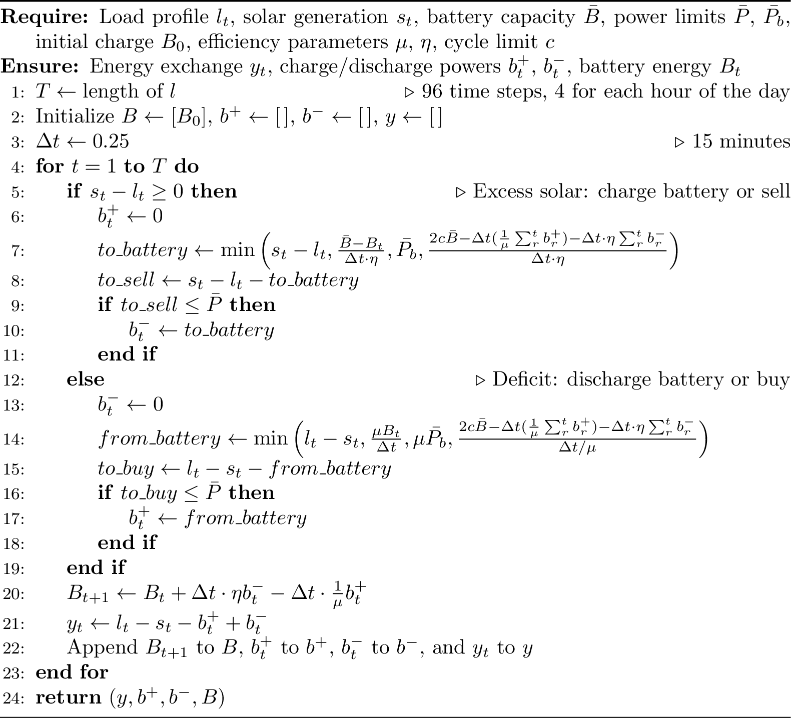
Algorithm 1 provides a heuristic for optimizing self-consumption in a PV-BESS. At each discrete time step \(t\), the algorithm determines the charge and discharge powers, \(b^{-}_t\) and \(b^{+}_t\), according to the instantaneous balance between solar generation \(s_t\) and load demand \(l_t\). When \(s_t \ge l_t\), the excess energy is first allocated to battery charging, limited by the remaining storage capacity \(\bar{B}\), the maximum charging power \(\bar{P_b}\), and the cumulative cycle constraint \(c\), taking into account the charging efficiency \(\eta\). Any residual energy that cannot be stored is exported to the grid, provided that the export power does not exceed \(\bar{P}\). Conversely, when \(s_t < l_t\), the energy deficit is initially compensated by discharging the battery, subject to the available stored energy \(B_t\), and the corresponding power and cycle limits, taking into account the discharging efficiency \(\mu\). If the remaining unmet demand after battery discharge is within the import limit \(\bar{P}\), it is supplied by purchasing energy from the grid. At each iteration, the battery state \(B_t\) is updated based on the realized charge and discharge flows, and the resulting grid exchange \(y_t\) is computed. The procedure iterates over all time periods, generating feasible trajectories \((y_t, b^{+}_t, b^{-}_t, B_t)\) that satisfy the operational constraints and approximate the optimal self-consumption policy under the given parameters. We will refer to this rule-based control strategy as the Automatic Battery (AB) model.
The main advantage of the AB model lies in its simplicity: it allows each user to operate autonomously based on local information, without the need for forecasts or centralized coordination. It is easily implementable in practice and guarantees that all technical constraints on storage and power flows are satisfied at each time step. However, this approach reacts only to instantaneous conditions of production and consumption. It does not anticipate future variations in load, solar generation, or grid conditions, nor does it consider external objectives such as carbon intensity minimization. As a result, although it enhances local self-consumption, it may lead to suboptimal performance when evaluated under stochastic operating environments.
In this work, we aim to move beyond this reactive strategy and apply a more systematic, optimization-based framework. Specifically, we formulate the problem as a set of stochastic linear optimization models, which determine the optimal quantities of energy to buy, sell, or store over a daily horizon. These models explicitly account for the uncertainty in household demand, solar production, and the carbon emission factor associated with purchased electricity. Since the emission intensity of grid energy varies dynamically with the generation mix, incorporating stochasticity allows the optimization process to identify strategies that minimize expected carbon emissions while preserving operational feasibility. We describe these models in the next section.
3 Carbon emissions optimization models↩︎
3.1 Programmed Battery model↩︎
We now formulate a stochastic optimization model focused on minimizing the carbon emissions. Let \(\Xi\) denote a finite set of possible scenarios \(\xi \in \Xi\), each representing a different realization of load demand \(l_{t,\xi}\) and solar generation \(s_{t,\xi}\) over the time horizon \(T\). In this setting, the control variables \(b_t^+\) and \(b_t^-\), representing the planned charge and discharge powers of the battery, are determined ex ante, before the actual realization of uncertainty. The objective is to program these quantities in such a way that the expected carbon emissions associated with the purchased energy \(y_{t,\xi}^+\) are minimized, while still satisfying all operational constraints on power flows, storage capacity, and battery cycling.
Unlike the AB model, which follows a purely reactive, rule-based logic, the Programmed Battery (PB) model optimizes battery operation in a forward-looking manner. It anticipates variability in solar production, demand, and emission intensity by considering the scenario set \(\Xi\). This allows the model to make proactive decisions that minimize the expected environmental impact rather than simply maximizing instantaneous self-consumption.
Formally, the PB model is written as a stochastic mixed-integer linear optimization problem, solved through Sample Average Approximation (SAA) [24] on the scenario set \(\Xi\). We can write it as follows: \[\tag{7} \begin{align} \min \quad &\Delta t \frac{1}{| \Xi |}\sum_{t \in T} \sum_{\xi \in \Xi}\alpha_{t,\xi}y_{t,\xi}^+ + \beta \cdot \Delta t \frac{1}{\mu}\sum_{t \in T} b_{t}^+ \tag{8}\\ \text{s.t.} \quad &y_{t,\xi}^+ - y_{t,\xi}^- = l_{t,\xi} - s_{t,\xi} - b_{t}^+ + b_{t}^- &&\forall t \in T, \, \xi \in \Xi, \tag{9}\\ &B_{0} - \Delta t \sum_{r=1}^{t} \left(\frac{1}{\mu}b_{r}^+ - \eta b_{r}^- \right) \geq 0 &&\forall t \in T,\\ &B_{0} - \Delta t \sum_{r=1}^{t} \left(\frac{1}{\mu}b_{r}^+ - \eta b_{r}^- \right) \leq \bar{B} &&\forall t \in T,\\ &\sum_{t \in T} \left( \frac{1}{\mu}b_{t}^+ - \eta b_{t}^-\right) = 0, & \tag{10}\\ &\Delta t \left(\frac{1}{\mu}\sum_{t \in T}b_{t}^+ + \eta \sum_{t \in T} b_{t}^-\right) \leq 2 c \bar{B}, &\\ & 0 \leq b^+_t \leq \mu \bar{P_b} (1-w_t) && \forall t \in T, \tag{11}\\ & 0 \leq b^-_t \leq \bar{P_b} w_t && \forall t \in T, \tag{12}\\ &0 \leq y_{t, \xi}^+, y_{t, \xi}^- \leq \bar{P} &&\forall t \in T, \, \xi \in \Xi, \tag{13}\\ & 0 \leq B_0 \leq \bar{B}, && \tag{14}\\ & w_t \in \{0,1\}, && \forall t \in T. \tag{15} \end{align}\]
In the objective function 8 , the first term represents the expected carbon emissions associated with electricity purchased from the grid, weighted by the time- and scenario-dependent emission factor \(\alpha_{t,\xi}\), which represents the grams of equivalent CO\(_2\) emitted per kilowatt-hour (gCO\(_2\)e/kWh), while \(\beta\) indicates the gCO\(_2\)e/kWh associated with the energy supplied by the storage battery (see [25] for a detailed discussion).
Constraints 9 –15 ensure the feasibility of power balance, storage dynamics, and operational limits across all scenarios. Note that Constraints 11 –15 avoid the simultaneous charging and discharging of the battery. These constraints are not needed for variables \(y^-\) and \(y^+\) because of the objective function, and under mild assumption, even the constraints for \(b^-\) and \(b^+\) can be discarded, see [26]. Note that the initial battery’s energy content \(B_0\) is a variable, and that Constraint 10 ensures that the final state of charge is equal to \(B_0\).
By integrating uncertainty into the optimization process, the PB model enables a more efficient and environmentally conscious management of distributed energy storage systems. In the next section, we derive a different battery model, again with planned charge and discharge quantities, starting from an idealized model.
3.2 Theoretical optimum and derivations↩︎
To establish theoretical performance benchmarks for our stochastic optimization framework, we consider a fully scenario-dependent formulation of the battery scheduling problem. This idealized model assumes that the decision-maker has perfect foresight of all future realizations of load, solar generation, and emission factors. Formally, it is obtained by extending model 7 and allowing the battery control variables to depend explicitly on the scenario, that is, by replacing \(b_t^+\) and \(b_t^-\) with \(b_{t,\xi}^+\) and \(b_{t,\xi}^-\). We refer to this formulation as the Omniscient Battery (OB) model.
The OB model represents the theoretical optimum of our system: it provides the lowest possible expected carbon emissions that could be achieved if all uncertainty were known in advance. Although such complete information is unrealistic in practice, the OB model serves two important purposes. First, it offers a lower bound on the optimal value of the realistic models, including the Programmed Battery (PB) model. Second, it allows us to derive a meaningful upper approximation for the PB model through an additional construct.
Specifically, we define the Mean Battery (MB) model, which uses the expected values of the scenario-dependent optimal decisions \(b_{t,\xi}^+\) and \(b_{t,\xi}^-\) obtained from the OB solution. In other words, the MB model replaces the scenario-dependent battery operation with fixed charging and discharging schedules \[b_t^+ = \frac{1}{|\Xi|}\sum_{\xi \in \Xi} b_{t,\xi}^+, \qquad b_t^- = \frac{1}{|\Xi|}\sum_{\xi \in \Xi} b_{t,\xi}^-,\] and evaluates their performance across all scenarios. This approach (if feasible) yields an upper bound on the expected cost of the PB model, as it represents a suboptimal policy derived from the omniscient solution.
Taken together, the OB and MB formulations delineate the theoretical limits of performance for stochastic battery scheduling. The OB model provides the best achievable benchmark under perfect information, while the MB model represents a practical approximation. In the following section, we will derive other meaningful models, where the charging and discharging powers at a time \(t\) depend on previous realizations of solar generation and load demand.
3.3 Feedback Battery models↩︎
In contrast to the OB and MB formulations, which assume either perfect foresight or fixed expected schedules, we now introduce a class of intermediate models that incorporate temporal feedback. In these models, the charging and discharging powers depend explicitly on the past realizations of load and solar generation, allowing decisions to adapt dynamically to the observed system behaviour while preserving linearity and tractability. This class of models will be referred to as Feedback Battery (FB) models.
The general idea is to represent the battery decisions as affine functions of the past observations of \(l_{r,\xi}\) and \(s_{r,\xi}\), for \(r < t\). Thus, we introduce variables \(\lambda, \, \phi, \, \psi\) representing the affine functions, and for each time step \(t\) and scenario \(\xi\), we express the control rules as \[\tag{16} \begin{align} b_{t,\xi}^+ &= \lambda_{t}^+ + \sum_{r=1}^{t-1} \left(\phi_{t,r}^+ l_{r,\xi} + \psi_{t,r}^+ s_{r,\xi}\right), & \forall t \in T, \, \xi \in \Xi, \tag{17}\\ b_{t,\xi}^- &= \lambda_{t}^- + \sum_{r=1}^{t-1} \left(\phi_{t,r}^- l_{r,\xi} + \psi_{t,r}^- s_{r,\xi}\right), & \forall t \in T, \, \xi \in \Xi, \tag{18}\\ & \lambda_{t}^+, \lambda_{t}^-, \phi_{t, r}^+, \phi_{t, r}^-, \psi_{t, r}^+, \psi_{t, r}^- \in \mathbb{R}, & \forall t,r \in T, r < t. \end{align}\] This complete formulation, hereafter denoted as FB0, provides the highest modeling flexibility. It allows the charging and discharging actions at time \(t\) to depend linearly on all past realizations of both load and generation up to time \(t-1\). However, this expressiveness comes at the cost of a large number of parameters, which may become computationally demanding for long horizons.
To reduce dimensionality, we propose two simplified versions of the feedback structure. The first relaxation, denoted as FB1, assumes that the feedback coefficients are time-invariant, i.e., they do not depend on the current period \(t\) but only on the index of the past observation: \[\label{eq:fb95relax1} \begin{align} b_{t,\xi}^+ &= \lambda_{t}^+ + \sum_{r=1}^{t-1} \left(\phi_{r}^+ l_{r,\xi} + \psi_{r}^+ s_{r,\xi}\right), & \forall t \in T, \, \xi \in \Xi,\\ b_{t,\xi}^- &= \lambda_{t}^- + \sum_{r=1}^{t-1} \left(\phi_{r}^- l_{r,\xi} + \psi_{r}^- s_{r,\xi}\right), & \forall t \in T, \, \xi \in \Xi, \\ & \lambda_{t}^+, \lambda_{t}^-, \phi_{t}^+, \phi_{t}^-, \psi_{t}^+, \psi_{t}^- \in \mathbb{R}, & \forall t \in T. \end{align}\tag{19}\] This specification preserves the dependence on individual past realizations but assumes that their influence is stationary over time.
Finally, the second relaxation, denoted as FB2, aggregates the past realizations of load and solar production through their cumulative sums. In this case, each battery decision depends only on the aggregated history of the observed variables: \[\label{eq:fb95relax2} \begin{align} b_{t,\xi}^+ &= \lambda_{t}^+ + \phi_{t}^+ \sum_{r=1}^{t-1} l_{r,\xi} + \psi_{t}^+ \sum_{r=1}^{t-1} s_{r,\xi}, & \forall t \in T, \, \xi \in \Xi,\\ b_{t,\xi}^- &= \lambda_{t}^- + \phi_{t}^- \sum_{r=1}^{t-1} l_{r,\xi} + \psi_{t}^- \sum_{r=1}^{t-1} s_{r,\xi}, & \forall t \in T, \, \xi \in \Xi, \\ & \lambda_{t}^+, \lambda_{t}^-, \phi_{t}^+, \phi_{t}^-, \psi_{t}^+, \psi_{t}^- \in \mathbb{R}, & \forall t \in T. \end{align}\tag{20}\]
Overall, the family of FB models bridges the gap between the fully anticipative OB and the scenario-independent PB formulations. By introducing linear feedback mechanisms, they capture partial adaptivity to stochastic realizations in a computationally tractable way.
4 Scenario generation↩︎
To properly capture the stochastic nature of load demand, PV generation, and grid carbon intensity, we generate a large number of synthetic daily scenarios starting from historical operational data. This section details the data preprocessing, normalization, scenario synthesis via Principal Component Analysis (PCA) [27], and the rationale behind the chosen sample size.
4.1 Data preprocessing and normalization↩︎
Following the methodology introduced in [26], we start from a collection of real daily profiles for each quantity of interest, i.e., electric load, PV production, and carbon intensity. Each signal is discretized over \(T = 96\) points, one for each quarter of an hour, producing a data matrix \(D \in \mathbb{R}^{n \times T}\), where each row corresponds to one daily realization.
Before applying PCA, the data are preprocessed to remove spurious values and measurement errors, and are normalized to make them comparable across users and magnitudes. For load demand and PV production, each profile is scaled by the nominal power of the user, ensuring that both quantities are expressed in per-unit terms relative to installed capacity. This normalization step preserves the relative dynamics while removing the effect of plant size. In the case of carbon intensity \(\alpha_t\), we apply a logarithmic transformation before normalization, i.e., \(\tilde{\alpha}_t = \log(\alpha_t)\), so that multiplicative variations in \(\alpha_t\) become additive in \(\tilde{\alpha}_t\). This guarantees that synthetic reconstructions of \(\alpha_t\) remain positive after back-transformation and that proportional variations are faithfully reproduced. After normalization, each column of the data matrix is centered to zero mean.
4.2 PCA and scenario synthesis↩︎
We then perform a singular value decomposition (SVD) [28] of the normalized data matrix, and retain the first five principal components, which together explain the vast majority of the total variance. Each component captures a dominant temporal pattern in the data, e.g., the morning and evening peaks in load, or the midday solar generation plateau.
To synthesize new, statistically consistent realizations, we sample random coefficients for each retained principal component. For component \(k\), the corresponding coefficient is drawn from a normal distribution \(\mathcal{N}(0, \lambda_k)\), where \(\lambda_k\) is the eigenvalue associated with that component. Each synthetic daily scenario \(\xi\) is then reconstructed as \[d_{\xi} = \bar{d} + \sum_{k=1}^{K} z_{\xi,k} u_k, \quad z_{\xi,k} \sim \mathcal{N}(0, \lambda_k),\] where \(\bar{d}\) is the mean daily profile and \(u_k\) are the retained principal directions. This procedure ensures that the generated profiles reproduce both the typical shape and the statistical dispersion observed in the empirical dataset.
After reconstruction, post-processing steps enforce physical feasibility: negative power values are truncated at zero, PV power is capped at the nominal system capacity, and carbon intensity values are obtained by exponentiating the reconstructed \(\tilde{\alpha}_t\). In our experiments, the fraction of truncated values is limited, and the resulting scenarios retain the main statistical features of the original data.
4.3 Scenario approach and number of samples↩︎
The number of generated scenarios \(M\) directly affects the statistical accuracy of the stochastic optimization models. To ensure theoretical reliability, we refer to the scenario approach formalism [29], whose mathematical foundation is summarized in [26]. Let \(\epsilon \in (0,1)\) denote an upper bound on the violation probability of the constraints. Under standard regularity assumptions, the following bound holds: \[\mathbb{P}^M \{ V(x^*_M) > \epsilon \} \leq \sum_{i=0}^{d-1} \binom{M}{i} \epsilon^i (1-\epsilon)^{M-i} \eqqcolon \tau,\] where \(d\) is the number of decision variables of the optimization problem, \(V(x^*_M)\) denotes the violation probability of the optimal solution \(x^*_M\) obtained from the sampled scenarios, and \(\tau\) denotes the confidence level [30], [31]. In our context, the decision space has a moderate dimension (hundreds of continuous variables), and a violation tolerance \(\epsilon = 0.01\) with confidence \(\tau = 10^{-5}\) leads to \(M=13{,}975\), therefore we generate \(14{,}000\) scenarios for our optimization purposes.
The resulting scenario set \(\Xi = \{ (l_{t,\xi}, s_{t,\xi}, \alpha_{t,\xi}) \}_{\xi=1}^{M}\) provides a discrete and statistically consistent approximation of the joint stochastic process governing user demand, PV generation, and carbon intensity. Using the same generation procedure, we construct a second independent set of scenarios, denoted by \(\Omega\), which is employed to evaluate the out-of-sample performance of the proposed models. The next section describes the computational experiments conducted to compare these models under the generated stochastic environments.
5 Computational results↩︎
Implementation details. All experiments were performed on a computer equipped with a 10th-generation Intel(R) Core(TM) i5 quad-core CPU and 16 GB of RAM. All functions were implemented in Python, and all linear optimization problems
were solved using the commercial solver Gurobi [32], version 11.0.1. The code developed for this study, which supports the results and analysis presented in
the article, is available in the repository “linear-battery-models” [33]. Parameters and data. We focus on
a single residential user equipped with a storage battery rated at \(5\) kW of power and \(13.5\) kWh of capacity, and a PV installation with a nominal power of \(6.4\) kWp. The following parameters are fixed throughout the experiments: \(\eta = \mu = 0.98\), \(c = 2\), and \(\beta =
32.9\) gCO\(_2\)e/kWh [25]. Two distinct sets of scenarios are generated, namely \(\Xi\) and \(\Omega\), the first being the set on which we optimize our models (which we will also call training set), the second being used to test out-of-sample performances (which we will also
call test set). In accordance with 4, we set \(|\Xi| = 14{,}000\) and a comparable number of test samples, that is \(|\Omega| = 10{,}000\), also taking
into consideration the confidence level \(\tau\). The data used to generate the samples \((l_{t,\xi}, s_{t,\xi}, \alpha_{t,\xi})\), \(\xi \in \Xi\), were
derived from Italian operational data in the period from 12 March 2025 to 12 April 2025. Solar generation and load demand were obtained from [34], [35], while the carbon intensity factor \(\alpha_t\) was computed based on the generation mix reported by [36]. The data used to generate the samples \((l_{t,\omega}, s_{t,\omega}, \alpha_{t,\omega})\),
\(\omega \in \Omega\), were obtained in the same way but using data in the period between 13 April 2025 and 13 May 2025. The time-shift structure reflects an operational setting in which decisions at time \(t\) are based only on past and current information. In particular, the control policy is constructed using historical data up to time \(t-1\), ensuring implementability in real-world
applications. The generated scenarios, instead, represent possible realizations of future uncertainty and are used exclusively for out-of-sample evaluation of the policy performance.
Although the experiments focus on a single representative user and a single day, similar results are observed for other profiles and time periods, as discussed in [26]. Some of these results are reported in 7. We now describe how each of the models introduced in 3 was tested. Automatic Battery. Since the AB model operates independently on each scenario and requires no parameter optimization, we directly run the self-consumption algorithm for every test scenario \(\omega \in \Omega\). We also run it for every training scenario \(\xi \in \Xi\) just for comparison purposes. Programmed Battery. The PB model is first solved on the training scenarios \(\xi \in \Xi\), yielding the optimal charging and discharging schedules \((b_t^+, b_t^-)\). These schedules are then fixed and the model is re-evaluated on the test scenarios \(\omega \in \Omega\) to assess out-of-sample performance. Omniscient and Mean Battery. The OB model provides a theoretical lower bound on achievable emissions, as it assumes perfect knowledge of future realizations. Hence, it is solved independently for each test scenario \(\omega \in \Omega\). For the MB model, we first solve the OB model on all training scenarios \(\xi \in \Xi\) and compute the expected values \(\mathbb{E}[b_t^+]\) and \(\mathbb{E}[b_t^-]\). These expected values are then fixed as deterministic control policies, and the model is re-run on each test scenario \(\omega \in \Omega\). We also run it for every scenario \(\xi \in \Xi\) just for comparison purposes. Feedback Battery. For each FB model (FB0, FB1, and FB2), we first solve the optimization problem on the training scenarios \(\xi \in \Xi\) and record the optimal feedback coefficients \(\lambda_t^{+}\), \(\phi^{+}_*\), \(\psi^{+}_*\), \(\lambda_t^{-}\), \(\phi^{-}_*\), and \(\psi^{-}_*\). These coefficients are then fixed, and the resulting feedback policy is evaluated on the test scenarios \(\omega \in \Omega\). Because of the large number of training scenarios, a standard SAA was computationally infeasible; instead, we employed an \(N\)-fold SAA approach [37]. Specifically, the set \(\Xi\) was divided into \(N\) disjoint subsets \(\Xi_1, \dots, \Xi_N\). For each subset \(\Xi_j\), an SAA was solved to estimate the feedback parameters, which were then tested on the complementary set \(\Xi \setminus \Xi_j\). This procedure can be fully parallelized across subsets. The parameter configuration yielding the best performance on the complementary set was selected and subsequently applied to the test set \(\Omega\). The number of folds \(N\) was set to \(140\) for FB0, \(70\) for FB1, and \(28\) for FB2, according to their decreasing computational complexity. Because FB0 and FB1 were the most expensive models, we imposed time limits on the optimization runs: \(2\) hours for FB0 and \(4\) hours for FB1.
| Optimization | Out-of-sample | ||||
| Model | Emissions | Time | Emissions | Gap (\(\%\)) | |
| OB | 1\(\,\)626.38 | 1h 11m 08s | 1\(\,\)357.58 | 0.00 | |
| AB | 2\(\,\)474.27 | 11s | 2\(\,\)016.10 | 48.51 | |
| PB | 1\(\,\)816.97 | 2m 48s | 1\(\,\)489.80 | 9.74 | |
| MB | 1\(\,\)891.64 | 1h 11m 09s | 1\(\,\)576.90 | 16.16 | |
| FB0 | 1\(\,\)691.27 | \(^\dagger\)2h 08m 08s | \(^*\)2\(\,\)527.44 | \(^*\)86.17 | |
| FB1 | 1\(\,\)787.05 | \(^\dagger\)4h 40m 20s | 1\(\,\)489.13 | 9.69 | |
| FB2 | 1\(\,\)810.96 | \(^\dagger\)15m 04s | 1\(\,\)490.86 | 9.82 | |
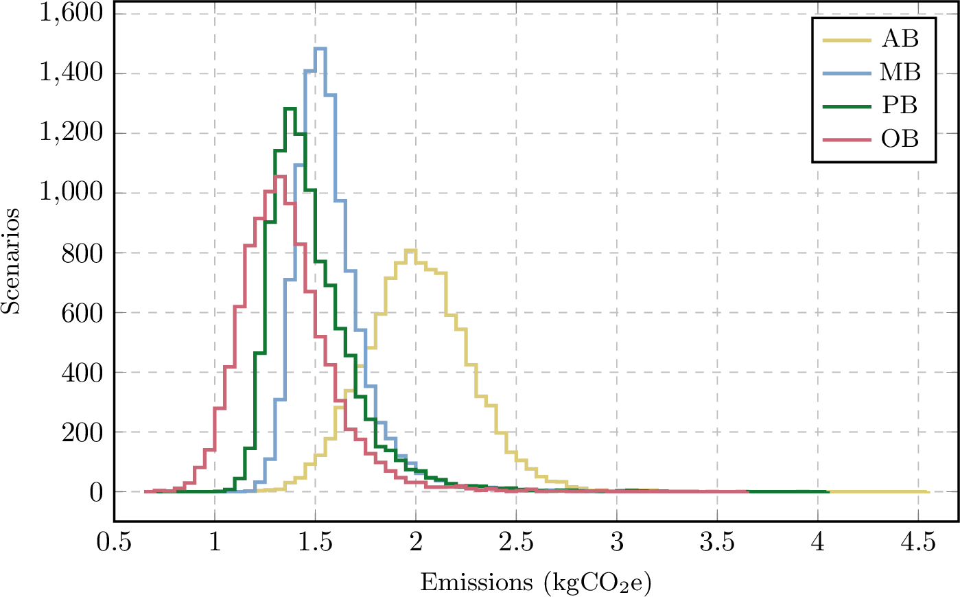
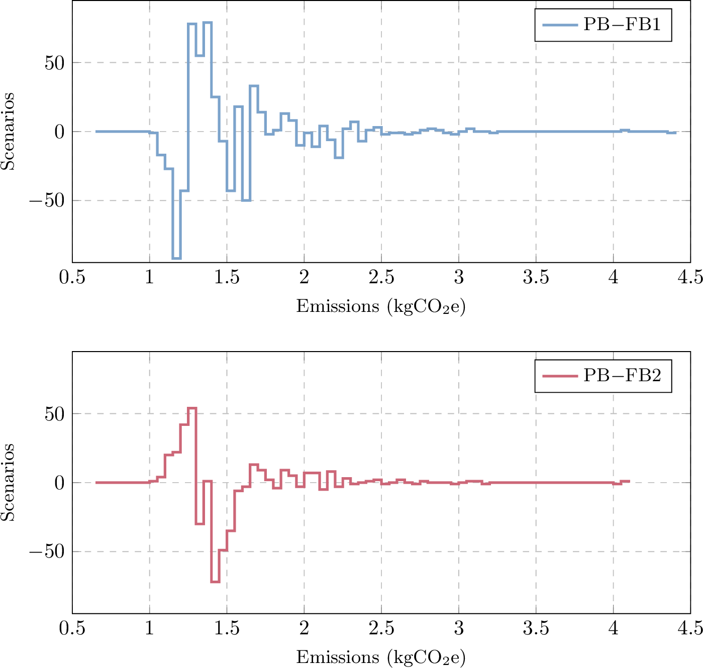
A comparative analysis of the total daily equivalent carbon emissions obtained under the different control strategies is summarized in 2 and visualized in [fig:distribution,fig:comparison]. The emission distributions across all test scenarios (Figure 2) clearly show the hierarchy among the proposed models. The OB assumes perfect foresight of all realizations, thus providing the theoretical lower bound, with an average of 1,357 gCO\(_2\)e per day. The PB achieves out-of-sample emissions of 1,490 gCO\(_2\)e, only \(9.74\%\) higher than the OB benchmark, while maintaining excellent computational efficiency (less than three minutes of runtime). The Feedback Battery models FB1 and FB2 perform nearly identically to PB, so we avoid showing their distribution profile on a graph. This similarity is instead illustrated in Figure 3, which reports the pairwise emission differences between PB, FB1, and FB2 across the test scenarios. For each emission interval, the curves show how many more (negative values) or fewer (positive values) scenarios fall within that range when compared to the PB model. Across all emission levels, the differences are minimal, below 100 scenarios per bin, confirming that FB1 and FB2 reproduce nearly the same statistical behaviour as PB. A closer inspection of the low-emission region shows that FB1 yields more low-emission scenarios than PB (so the PB\(-\)FB1 curve is negative in the \(1.0\)-\(1.2\) kgCO\(_2\)e range), whereas FB2 yields fewer low-emission scenarios than PB (so the PB\(-\)FB2 curve is positive there). In other words, FB1 is marginally better than PB at producing very low-emission outcomes, while FB2 is marginally worse, but the magnitude of these effects is small and does not materially change the overall distribution shape.
The MB, in which charging and discharging schedules are fixed to the average optimal profiles computed over the training set, results in approximately \(16\%\) higher emissions than OB and \(6\%\) higher than PB. The AB, based on simple rule-based self-consumption, performs substantially worse, producing roughly \(36\%\) higher emissions than the PB model and more than \(48\%\) higher emissions than the OB benchmark. Although its computational time is negligible (about 11 seconds per scenario), its purely reactive strategy leads to much higher carbon intensity due to inefficient use of stored energy.
The matrix-form Feedback Battery (FB0), which models a full temporal dependence of charging and discharging powers on past load and solar realizations, exhibits severe feasibility issues. Because the model’s parametrization involves a large number of decision variables, it required an \(N\)-fold SAA procedure with a reduced number of training scenarios. While the optimization gives good results on unseen training data, the model fails on test data both in terms of feasibility (6,412 out of 10,000 test scenarios resulted in infeasibility) and optimality, being the model with the highest average emissions on out-of-sample scenarios.
Overall, the results demonstrate that moderate feedback complexity can improve training performance but provides no tangible advantage on unseen data. Among all practical formulations, the PB model achieves the best compromise between computational efficiency, robustness, and emission minimization, approaching the theoretical lower bound while remaining feasible across all scenarios.
6 Conclusions↩︎
This work investigated several linear optimization frameworks for the operation of PV-battery systems under uncertainty, with the goal of minimizing equivalent carbon emissions. A hierarchy of models was developed, ranging from simple rule-based control (Automatic Battery) to stochastic optimization with feedback-dependent battery behaviour (Feedback Batteries). The models were tested on large sets of synthetic scenarios generated via PCA of real Italian data, encompassing variability in load, solar production, and grid emission intensity.
The comparative analysis showed that direct minimization of expected emissions through stochastic programming (Programmed Battery) achieves significantly lower emissions than traditional self-consumption heuristics. Introducing temporal feedback into battery control can further improve training performance, but the gains vanish on unseen scenarios and come at the cost of substantially higher computational complexity. The Omniscient Battery model provides a theoretical lower bound, while the Mean Battery model illustrates that averaging control profiles across scenarios is not an effective strategy. Among practical formulations, the PB model remains the most robust and computationally tractable approach. Additional experiments on winter data (December 2025), reported in 7, confirm the robustness of these findings across seasons. The relative ranking of the models is preserved: PB consistently outperforms AB, with performance close to OB. However, the differences among all models are far less pronounced than in spring: the gap between AB and OB drops from approximately \(48\%\) to just \(11\%\), and PB, FB2, and AB all cluster within \(11\)–\(11.3\%\) of the OB lower bound. This convergence reflects the reduced solar generation available during winter, which limits the charging opportunities for the battery and shrinks the decision space for optimal scheduling. The practical implication is that the benefit of stochastic optimization over simple self-consumption is strongly modulated by the available renewable resource, and is most impactful during seasons with abundant photovoltaic generation.
Future research should focus on extending this analysis in several directions. First, non-linear feedback laws could be explored to better capture the complex relationships between battery operation, load dynamics, and solar generation without relying on purely linear dependencies. Second, the aggregation of multiple users into Renewable Energy Communities (RECs) represents a promising avenue for future work. By coordinating battery operation and renewable generation across several users, RECs could exploit spatial and temporal complementarities to further reduce emissions and enhance grid flexibility. Finally, the inclusion of environmental or economic trade-offs, such as multi-objective optimization balancing emissions, costs, and battery degradation, would enhance the realism and policy relevance of the proposed models.
Overall, this study demonstrates the potential of stochastic linear optimization to significantly reduce carbon emissions from distributed PV systems, while highlighting the challenges of scalability and generalization that motivate future research on community-level and non-linear control strategies.
7 Extensive computational results↩︎
To assess the robustness of the proposed models across different seasonal conditions, we replicate the computational experiments described in 5 using winter data from December 2025. The data were obtained from [34], [35] and processed following the same methodology outlined in 4. Synthetic scenarios were generated using the PCA-based procedure described in 4, retaining \(K = 5\) principal components. The training set consists of \(14{,}000\) scenarios (\(|\Xi| = 14{,}000\)), while the test set comprises \(10{,}000\) scenarios (\(|\Omega| = 10{,}000\)). Compared to the spring data used in the main experiments, winter profiles exhibit lower and shorter solar peaks, higher average loads (due to heating demand), and slightly different carbon intensity patterns.
3 reports the expected daily emissions for each model. For each model, we report the total expected emissions obtained in the optimization stage, the corresponding computation time, and the out-of-sample emissions computed on \(10{,}000\) test scenarios. The “Gap” column measures the percentage increase in out-of-sample emissions relative to the OB benchmark. Among the feedback models, only FB2 is included in the winter experiments. As shown in 5, FB1 achieves out-of-sample performance very similar to FB2 but requires significantly longer computation time (\(4\)h \(40\)m vs.\(15\)m per block in spring), while FB0 suffers from poor out-of-sample generalization due to overfitting. Since the winter regime further reduces the gap among all models, the marginal differences between FB1 and FB2 become negligible, making FB2 the natural representative of the feedback family.
For the FB2 model, we followed the same SAA cross-validation procedure used in the main experiments: the \(14{,}000\) training scenarios were partitioned into \(28\) blocks of \(500\) scenarios each; FB2 was solved independently on each block, and the resulting feedback coefficients were evaluated on the remaining \(13{,}500\) training scenarios. The block with the lowest cross-validation emissions was selected, and its coefficients were used for the final out-of-sample evaluation. The computation time reported for FB2 corresponds to the longest single block optimization (since all 28 blocks can be solved independently in parallel).
| Optimization | Out-of-sample | ||||
| Model | Emissions | Time | Emissions | Gap (\(\%\)) | |
| OB | 3\(\,\)795.61 | 18m 10s | 2\(\,\)443.98 | 0.00 | |
| AB | 3\(\,\)958.69 | 7s | 2\(\,\)720.95 | 11.33 | |
| PB | 3\(\,\)942.00 | 10m 30s | 2\(\,\)712.53 | 10.99 | |
| MB | 4\(\,\)016.83 | 18m 10s | 2\(\,\)875.18 | 17.64 | |
| FB2 | 4\(\,\)040.45 | \(^\dagger\)12m 52s | 2\(\,\)718.68 | 11.24 | |
A comparative analysis of the total daily equivalent carbon emissions obtained under the different control strategies is summarized in 3 and visualized in 4. The emission distributions are presented as box plots rather than overlaid histograms (as in 2), since the close overlap among models in the winter regime makes individual histogram curves difficult to distinguish. Notably, the optimization emissions are substantially higher than the out-of-sample emissions. This is explained by the underlying meteorological data: the training period exhibited significantly lower solar irradiance (average daily PV generation approximately \(45\%\) lower than the test period), resulting in less self-consumed solar energy and higher grid imports during training. The most striking feature of the winter results is the substantially narrower spread among models compared to the spring experiments (2). All models except MB achieve out-of-sample emissions within approximately \(11\%\) of the OB lower bound, whereas in spring the gap between AB and OB exceeded \(48\%\). This compression is a direct consequence of the reduced PV generation during winter months: with less surplus solar energy available, the battery has fewer charging opportunities, and the decision space for optimal scheduling shrinks. As a result, even the simple self-consumption heuristic (AB) operates close to optimality, leaving little room for improvement through stochastic optimization. The OB model provides the theoretical lower bound, with an average of \(2{,}443.98\) gCO\(_2\)e per day. The PB model achieves out-of-sample emissions of \(2{,}712.53\) gCO\(_2\)e, \(10.99\%\) above OB. The FB2 model, trained via 28-block SAA cross-validation, yields \(2{,}718.68\) gCO\(_2\)e (\(11.24\%\) above OB), closely matching PB and confirming that the additional feedback parameters do not provide significant generalization gains, particularly in a low-solar regime where the battery control problem is inherently simpler. The AB model results in \(2{,}720.95\) gCO\(_2\)e (\(11.33\%\) above OB), only marginally worse than PB and FB2. The MB model, at \(2{,}875.18\) gCO\(_2\)e (\(17.64\%\) above OB), is the only model with a noticeably larger gap, confirming that averaging optimal control profiles across scenarios is not an effective strategy regardless of the season.
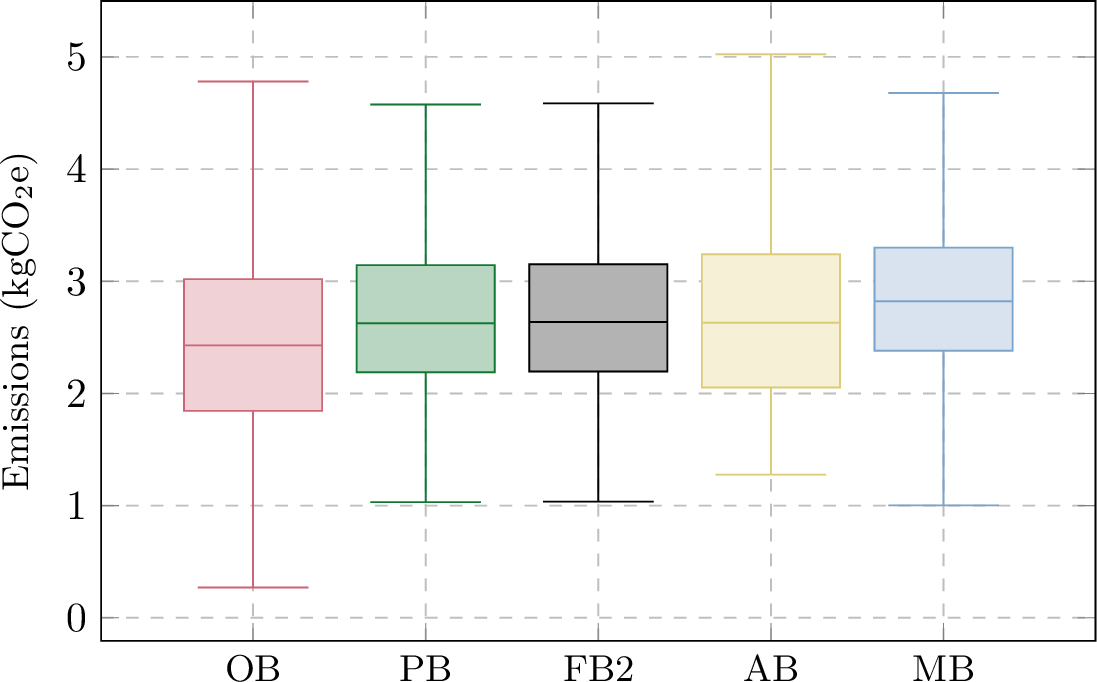
Overall, the winter experiments confirm that the relative ranking of the models is preserved across seasons: stochastic optimization (PB) consistently outperforms rule-based control (AB), with performance close to the omniscient lower bound (OB). However, the differences among AB, PB, and FB2 are far less pronounced than in the spring case (gaps of \({\approx}\,11\%\) vs.OB, compared to \(13\)–\(48\%\) in spring). This convergence reflects the reduced PV resource available during winter: with fewer charging opportunities for the battery, the decision space for emission-reducing scheduling shrinks, and even simple heuristics operate near-optimally. The practical implication is that the benefit of stochastic optimization over self-consumption is strongly modulated by the available solar resource, and is most impactful during seasons with abundant and variable photovoltaic generation.
Declaration of competing interest↩︎
The authors declare that they have no known competing financial interests or personal relationships that could have appeared to influence the work reported in this paper.
Data availability↩︎
The energy load and solar generation data used in this study are publicly available from the Transparency Platform of [34], [35] and from [36]. The source code and data processing scripts are available at [33].