Moebius: Serving Mixture-of-Expert Models
with Seamless Runtime Parallelism Switch
June 25, 2026
Abstract
Mixture-of-Experts (MoE) architectures scale large language models (LLMs) to hundreds of billions of parameters. Serving a single MoE model requires multiple GPUs operating in parallel, typically through tensor parallelism (TP) or expert parallelism (EP). The optimal choice depends on the number of in-flight requests: TP is faster at low concurrency, whereas EP wins at high concurrency. Production workloads cross this boundary continually: online serving sees bursty arrivals that subside into quiet periods, and reinforcement-learning rollouts begin as a high-concurrency burst that decays into a long tail of stragglers. Pinning either layout therefore forfeits performance when the workload crosses to the other side.
We present Moebius, a serving system that switches between EP and TP at runtime without restarting the engine or dropping in-flight requests. Our key insight is that EP and TP are two layouts of one model, not two models: they compute the same function over byte-identical expert weights and KV cache, so a switch changes only which rank owns each slice. Moving those owner-changed slices is the sole irreducible cost, and modern high-bandwidth GPU interconnects make it fast enough to do between decode steps without draining in-flight requests. Moebius preserves each parallelism’s runtime resident, and reshards the single copy of expert weights and KV cache at fixed addresses with fused GPU-to-GPU transfer kernels. On 8\(\times\)H200 GPUs serving Qwen3-235B-A22B, Moebius matches the better static parallelism at every operating point, and beats it on RL rollouts by 1.16–1.25\(\times\) across steps. Each switch completes in 215–434 ms, and Moebius holds both layouts resident with only 2.4% memory overhead.
1 Introduction↩︎
![Figure 1: Optimal parallelism for MoE decoding shifts with the active load. (a) Measured decode latency vs concurrency (i.e. global batch size) for TP, EP, and Moebius on a static load sweep (8\timesH200, Qwen3-235B). The switch point marks the TP–EP crossover. (b) Request arrival rate (req/s) over time on an Azure online serving trace [1] (top) and a bursty trace (bottom). Vertical markers indicate switch points between TP and EP. (c) The same RL rollout batch runs on TP, EP, and Moebius. Each white strip is one sample’s decode lifetime, with length proportional to the number of its output tokens. An initial burst transitions to the long tail phase when most samples finish and only a few stragglers are still running. Background shading marks the two phases, and Moebius switches EP\rightarrowTP at the boundary.](/article/2606.26607/_pdflatex/njmbfocw.png "fig:")
Mixture-of-experts (MoE) [2] has become a leading architecture for scaling large language models (LLMs). By activating only a small subset of expert sub-networks per token, an MoE model grows to hundreds of billions of parameters without a proportional increase in per-token computation. Recent frontier models such as Qwen-MoE [3], DeepSeek [4], and GPT-OSS [5], together with the serving systems [6]–[8] that efficiently host them, have made MoE inference a mainstream deployment target.
During MoE inference serving, a parallelism configuration defines how the MoE model weights are distributed across GPUs. Tensor parallelism (TP) shards each expert and the attention heads across all GPUs, runs the full batch on every GPU, and
synchronizes partial results with per-step All-Reduce communication. Expert parallelism (EP) assigns each GPU a subset of experts together with a disjoint slice of requests, routes tokens to their expert-owning GPUs with
All-to-All dispatch, and combines the results.
We observe that the optimal parallelism is critically dependent on the serving concurrency, as demonstrated in Figure 1 (a). A fixed parallelism is not uniformly preferable. At low concurrency, EP fragments the batch across
GPUs and leaves each rank with too little work to keep its kernels and attention efficient. At high concurrency, TP suffers both from the per-layer All-Reduce on the full hidden state and from larger per-rank MoE activation traffic. Real-world
workloads vary in concurrency over time, requiring runtime switching. Online serving traces exhibit bursty arrivals followed by quiet periods, repeatedly carrying the active batch across the TP–EP crossover and back (Figure 1
(b)). Beyond online serving, reinforcement learning (RL) rollouts such as GRPO [9] and DAPO [10] exhibit an even sharper variation: each rollout begins as a high-concurrency burst that favors EP and then decays into a long tail of stragglers that favors TP as sequences finish at different lengths [11], [12] (Figure 1 (c)). Applying a fixed TP or EP
layout to such dynamic workloads wastes the advantages of the other.
One might hope to reuse the runtime-switching approaches developed for dense LLM serving [13]–[15]. These systems, however, assume weights of both parallelisms are local on device, in-flight requests can be paused or drained, and runtime is cheap enough to rebuild. A production-level MoE serving system denies these assumptions, posing the following challenges for workload-adaptive parallelism switching.
Larger weight transfer. Expert weights are much larger than those of dense LLMs. The weights of only one parallelism layout can stay alive on device. Thus, a switch must reshard GPU-resident experts across the interconnect.
Requests resume. EP partitions requests across GPUs, while TP makes every GPU serve the full requests with sharded heads; therefore, a live switch must also redistribute in-flight requests and their paged key-value (KV) cache [7] to resume the decoding.
Graph-based execution. Nowadays, graph-based execution with pre-capturing (i.e., CUDA graph) is a de facto standard for low-latency serving. Tensor addresses are embedded in the graph, and a switch must not rewrite the captured addresses of the weights and cache.
To address these challenges, we present Moebius, the first MoE serving system that switches between EP and TP at runtime without draining in-flight requests. At first glance, such a switch looks expensive on every count: it appears to demand replicating/reloading gigabyte-scale expert weights, redistributing live requests, and recapturing CUDA graphs on every layout change.
Our key insight is that on modern high-bandwidth GPU interconnects such as NVLink, expert weights need no longer be treated as fixed assets: EP and TP are two layouts of one model, computing the same function over byte-identical weights and KV, and differing only in how that state is sharded across GPUs and which collectives move it. A parallelism switch is therefore not intrinsically expensive: its only irreducible cost is moving the data whose owners change. Moebius minimizes the cost: it keeps the control plane (CUDA graphs, communication groups, attention metadata) resident for both layouts, and reshards the data plane (expert weights, paged KV cache) over a single fixed-address allocation, so a switch selects the prepared runtime and moves only the owner-changed bytes.
Moebius realizes this design with three mechanisms. To manage the unchanged shared state between EP and TP, we use a unified memory manager. It pre-allocates contiguous storage for expert weights, KV cache, request buffers, and transfer scratch, exposing stable parallelism-specific tensor views, so captured CUDA graphs remain valid across switches. To provide a lightweight switch while supporting redistribution of in-flight requests, fused direct-transfer kernels move expert slices and KV shards directly into peer-GPU destination slots over GPU network, avoiding staged collective buffers and auxiliary on-device memory copy. Integrated with the above components, to support graph-based execution for low-latency serving, runtime-preservation mechanisms keep both parallelisms’ CUDA graphs, communication groups, and attention metadata resident, so that a switch selects prepared runtime state rather than rebuilding it.
We benchmark Moebius on 8\(\times\)H200 GPUs serving Qwen3-235B-A22B. Across a concurrency sweep of MoE serving as a microbenchmark, Moebius matches the better static layout at every operating point, as briefly shown in Figure 1 (a). On dynamic workloads, Moebius provides significant performance improvement with low switching overhead. On RL rollouts, it is the fastest at every rollout step, beating even an oracle that picks the better static layout per step by 1.16–1.25\(\times\), and either fixed baseline by up to 1.31\(\times\). On a bursty online-serving trace, it switches frequently between TP and EP with low overhead, improving both the prefill-bound time-to-first-token during bursts and the decode-bound time-per-output-token in the quiet periods. In these benchmarks, each switch completes in 215–434 ms. The direct-transfer kernel reshards expert weights in 152 ms, 1.49\(\times\) faster than an NCCL collective. Holding both layouts resident stays below static TP and within 0.2 GB of static EP, its 2.4% dual-mode buffer funded by shrinking the KV cache rather than adding memory. This paper makes the following contributions:
We show that the optimal parallelism layout crosses between TP and EP within a single serving episode, across a load sweep and through the burst-to-tail decay in RL rollouts. Parallelism must therefore be chosen at runtime rather than fixed at deployment, yet no existing serving system switches between EP and TP live during decode.
To support dynamic switching between EP and TP, we define a bidirectional transformation that reshards expert weights and migrates in-flight requests with their paged KV cache across the two layouts’ different attention shardings, producing outputs equivalent to those the destination layout would produce without draining the engine or recomputing any request.
We design, implement, and evaluate Moebius, which realizes the transformation through fixed-address unified memory buffer that keeps captured CUDA graphs valid, direct GPU-to-GPU transfer kernels that reshard \(1.49\times\) faster than an NCCL collective, and resident dual runtimes that are selected rather than rebuilt, switching in 215–434 ms at roughly 2.4% memory overhead.
2 Background and Motivation↩︎
2.1 Parallelism for MoE Inference↩︎
MoE inference factors into two independent placement choices. Attention can be tensor-parallel (TP), where every GPU holds the full batch with sharded heads, or data-parallel (DP), where each GPU owns a disjoint request slice and
stores the KV cache for only that slice. Experts can be tensor-parallel, where each weight matrix is sharded with All-Reduce [16], or expert-parallel (EP), where each GPU owns a subset of experts and tokens are routed via All-to-All [17]–[19]. The cross product gives four layouts, written attention/expert: TP/TP, DP/EP, DP/TP, and TP/EP. TP attention also
replicates the KV cache when the model has fewer KV heads than TP ranks, capping request capacity.
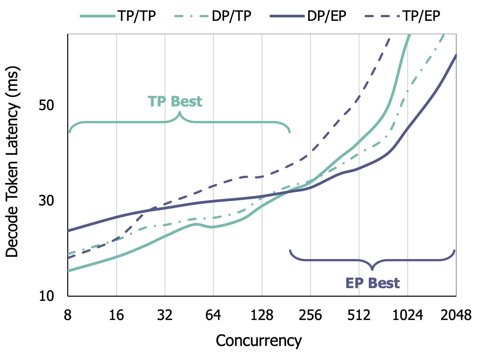
The favorable layout depends on load. We swept steady-state decode concurrency on Qwen3-235B-A22B across 8\(\times\)H200 GPUs with CUDA graphs enabled, measuring per-step decode latency for each of the four layouts. Across global batch sizes \(B\) from 8 to 2048, TP/TP won by \(1.5\times\) at small batches and DP/EP won by \(1.5\times\) at large batches (Figure 2), with the boundary between \(B{=}128\) and \(B{=}256\). The mixed layouts never joined the lower envelope, for structural reasons: DP/TP gathers the full token set before running TP experts and so misses DP/EP’s MoE-volume reduction, while TP/EP keeps TP attention’s full-token batch and feeds every token through the routing layer, erasing the activation-volume savings EP exists to provide. The rest of the paper therefore focuses on the two survivors, which we write TP for TP/TP and EP for DP/EP. The two are separated by a load-dependent boundary that production workloads must cross at runtime.
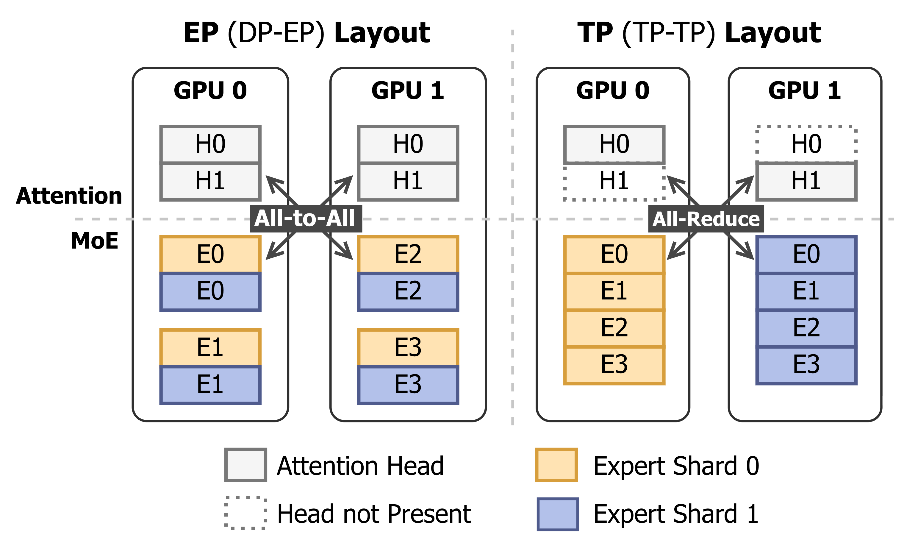
Why the boundary exists. TP and EP differ along two axes, each of which flips direction as \(B\) grows (Figure 3). The first is communication: TP’s per-layer All-Reduce ships the full hidden state and grows with \(B\), while EP’s All-to-All carries only routed tokens but pays a small-message dispatch floor that dominates when \(B\) is low. The second is MoE compute: decode MoE GEMMs are
memory-bound, so per-rank runtime tracks per-rank token count, which is \(B\) under TP and \(B/G\) under EP, where \(G\) is the EP group size. Both axes favor TP at small \(B\) and EP at large \(B\), and the boundary
sits where their crossovers compound.
The crossover is hardware- and model-agnostic. Both axes are structural, not artifacts of our model and GPU count: All-Reduce volume and the memory-bound \(B\) versus \(B/G\) compute gap hold for any MoE on any interconnect. Public benchmarks spanning many models and GPU generations show the same latency-throughput frontier, its tight-latency end served by TP and
its high-throughput end by EP [20].
2.2 Real World Workloads Cross the Boundary↩︎
Production workloads do not sit on one side of the TP–EP boundary. Two dominant deployment scenarios, bursty online serving and reinforcement-learning (RL) rollouts, drive the active batch across it.
Bursty online serving. Production LLM traces exhibit bursty arrivals separated by long quiet periods [1], [21], with peak in-flight counts spanning two to three orders of magnitude over minutes. A single deployment therefore crosses the boundary repeatedly. EP sustains the throughput required to drain bursts that would saturate TP, while TP delivers the per-token latency that interactive serving demands during quiet periods.
RL rollouts. RL post-training algorithms such as GRPO [9] and DAPO [10] interleave policy updates with rollout steps, and each step is itself a serving workload. A step submits a batch of prompts, samples each prompt multiple times for group-relative advantage, and decodes every sample to completion before the next weights update, so the engine sees thousands of in-flight requests at the burst peak. Per-request output lengths vary by more than an order of magnitude across the batch, since reasoning chains terminate at different points and a small fraction run all the way to the multi-thousand-token cap [10], [22]–[25]. The active batch therefore starts well above the boundary, decays through it, and lingers in a long tail of stragglers.
Different RL framework designs handle this tail differently, but none lift the burden from the generation engine. Synchronous (on-policy) frameworks [11], [12], [26] wait for the full tail before each weights update, since on-policy training requires every sample to come from the current weights and so accepts the long-tail cost as the price of training on its own outputs. Asynchronous (off-policy) systems [24], [27], [28] relax this constraint by overlapping the tail of one step with training on the previous step, reclaiming GPU cycles but leaving each rollout step’s workload shape unchanged, so the generation engine still observes the same burst-to-tail decay. Partial rollout, another off-policy approach, sidesteps the tail by truncating long generations and resuming them in a later step [28], [29], but a single response then spans multiple policy versions, which slows convergence in practice [24]. Outside the partial-rollout regime, every step’s in-flight count crosses the TP–EP boundary mid-step, and the generation engine benefits from following the favorable layout regardless of the surrounding framework.
2.3 Prior Switching Does Not Transfer to MoE↩︎
The workloads in §2.2 call for an engine that switches between TP and EP. Runtime switching is not new: dense-model systems already reconfigure layouts under shifting load (Shift Parallelism [13], Amoeba [14], Flying Serving [15]). Their designs assume what MoE denies: that weights stay resident, that the engine can be drained, and that the runtime is free to rebuild. A live MoE switch breaks all three.
Weights does not stay resident: a dense TP shard is a \(1/P\) slice of the data-parallel replica, so a system that keeps the replica already owns every TP shard without a reshard [13]–[15], but MoE experts dominate the model and EP and TP partition them along orthogonal axes that share no bytes, so a switch must reshard experts across GPUs without holding both copies. The engine cannot be drained: prior systems let in-flight requests finish or discard them [13], [15], whereas a live switch must carry the decode batch and its paged KV cache across EP’s and TP’s attention layouts without losing work. The runtime is expensive to rebuild: each layout’s attention metadata [30], [31], communication buffers [17]–[19], and CUDA graphs take tens of seconds to rebuild and stall every request, so a live switch keeps them resident instead.
3 Adaptive Parallelism↩︎
Decode batch size shifts as requests arrive and complete, so neither mode stays efficient for long. Moebius therefore treats the parallelism mode as runtime-reconfigurable state rather than a deployment-time constant. We write EP\(\to\)TP and TP\(\to\)EP for the two switch directions and EP\(\leftrightarrow\)TP when the direction does not matter. The key observation is that an EP\(\leftrightarrow\)TP switch only changes ownership: the model weights, in-flight requests, and KV values are the same before and after the switch across the all ranks. What changes is which rank owns each slice and which mode-specific view each rank uses for subsequent steps.
3.1 Weights Resharding↩︎
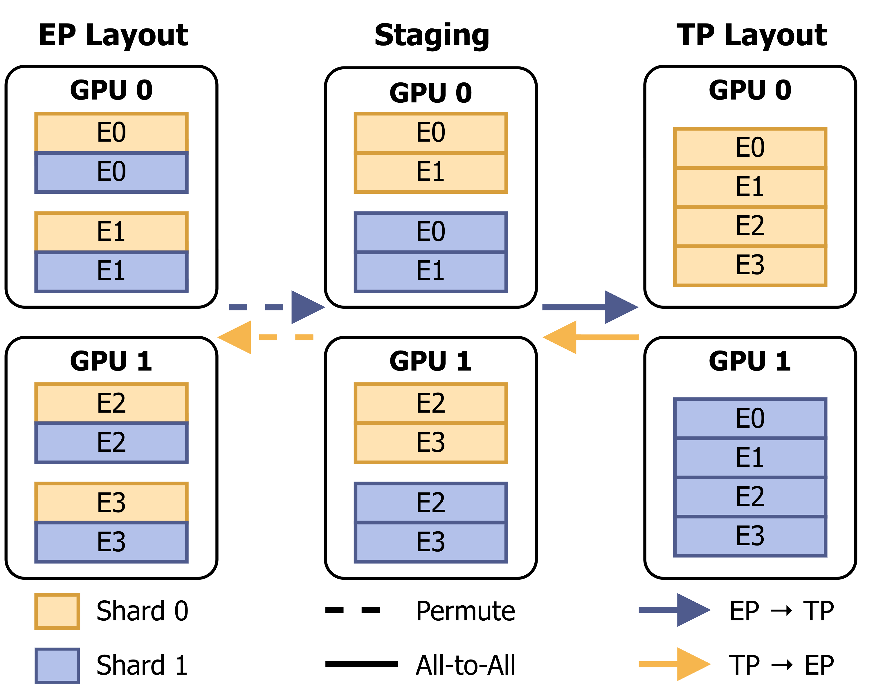
Let \(E\) be the total number of experts, \(P\) the number of ranks in the switching group, \(H\) the hidden size, and \(I\) the expert intermediate size. EP and TP store the same global expert weights but assign ownership differently. Under EP, each rank owns a disjoint subset of complete experts. It owns \(E_\text{local}=E/P\) experts and stores the full gate-up projection \(W_{13}\) with shape \((E_\text{local}, 2I, H)\), where the leading factor of two stacks the gate and up projections of the SwiGLU MLP, and the full down projection \(W_2\) with shape \((E_\text{local}, H, I)\). Under TP, each rank owns one shard of every expert: \(W_{13}\) has shape \((E, 2I/P, H)\), and \(W_2\) has shape \((E, H, I/P)\). A switch therefore changes which rank owns each slice and which tensor view the forward path uses; it does not change the global weight values.
A reshard decomposes into three possible stages: a local permute that packs outbound bytes into one contiguous chunk per destination peer, an All-to-All that transfers ownership across the global communication group, and a local scatter
that writes inbound bytes into the target layout. Weight resharding needs only two stages in either direction (Figure 4). EP\(\to\)TP runs permute then exchange: Moebius packs each
rank’s complete experts into per-peer chunks, and the All-to-All delivers each rank its shard of every expert already in place. TP\(\to\)EP runs exchange then permute: the All-to-All delivers
contiguous expert blocks, and the local permute interleaves the received shards into complete experts. The gate-up and down projections reshard symmetrically, along the output and input intermediate dimensions, respectively.
Attention weights are small compared with expert weights, so Moebius handles them separately. Under EP, attention is data-parallel and every rank holds the full query, key, value, and output projections. Under TP, attention is tensor-parallel and each
rank holds only its head shard. By default, Moebius keeps both layouts resident and switches attention weights by pointer swap, paying one duplicated head shard per rank. A memory-saving variant keeps only the active layout and rebuilds TP\(\to\)EP with an All-Gather.
3.2 Request Redistribution↩︎

Requests and their KV cache follow the attention layout, so a switch rewrites ownership of both while preserving the request state and KV values. Under EP, attention is data-parallel: each rank owns a disjoint subset of in-flight requests and stores their KV cache for every head. Under TP, attention is tensor-parallel: every rank serves every request but stores only its slice of the KV heads (Figure 5). When a model has fewer KV heads than ranks, TP replicates each head across a group of ranks. For example, Qwen3’s four KV heads [3] at TP 8 place two ranks per head. Request ownership is only host-resident metadata; the KV cache is large, GPU-resident, and costly to move.
In the EP\(\to\)TP direction, Moebius first reassigns request ownership with a metadata All-Gather: each rank contributes its running and waiting requests, and all ranks construct the same ordered list of
in-flight work. Moebius then repartitions the KV cache by attention head, leaving each rank with one head shard of every request rather than all heads of its own requests.
Paged attention complicates this transfer. KV cache is stored in fixed-size blocks drawn from a shared pool, so a request’s tokens occupy non-contiguous slots tracked by a page table, and distinct requests interleave arbitrarily [7]. Moving the cache request by request would launch thousands of tiny transfers per layer. Moebius instead reads the page tables and precomputes one index vector over every token a
rank must send. It then gathers the scattered slots into contiguous per-peer chunks, exchanges those chunks with one All-to-All, and scatters the received heads into target pages reallocated under TP. Unlike weight resharding, KV transfer
keeps all three stages because paging scatters both the source and destination slots.
The TP\(\to\)EP direction uses the same cache-transfer stages but changes request ownership. Instead of gathering requests onto every rank, Moebius partitions the global request list into disjoint per-rank subsets. It sorts requests by decreasing sequence length and greedily places each request on the least-loaded rank, balancing request and token counts together. The heuristic is deterministic, so every rank computes the same partition without communication. Each rank then sends its head shard of every departing request to that request’s new owner, which reassembles the full set of heads.
The switch runs synchronously across ranks while decode is paused between iterations. Request metadata, sampling state, and KV values migrate together, so no request is dropped and each resumes decoding at the same position. Waiting requests carry no KV cache, so the switch remaps only their ownership to the target layout.
4 System Design↩︎
Building on the switch definition in §3, Moebius must execute each EP\(\leftrightarrow\)TP transition as a low-latency serving operation rather than an offline reconfiguration. A practical switch faces four systems challenges, in the order addressed below: avoiding a second copy of model weights and KV cache, minimizing switch latency for expert-weight and KV-cache movement, preserving CUDA graphs and other mode-specific runtime state, and finding a proper point to switch. This section describes how Moebius addresses these challenges with its memory layout, fused direct-transfer kernels, runtime preservation, and switch policy.
4.1 Overview↩︎
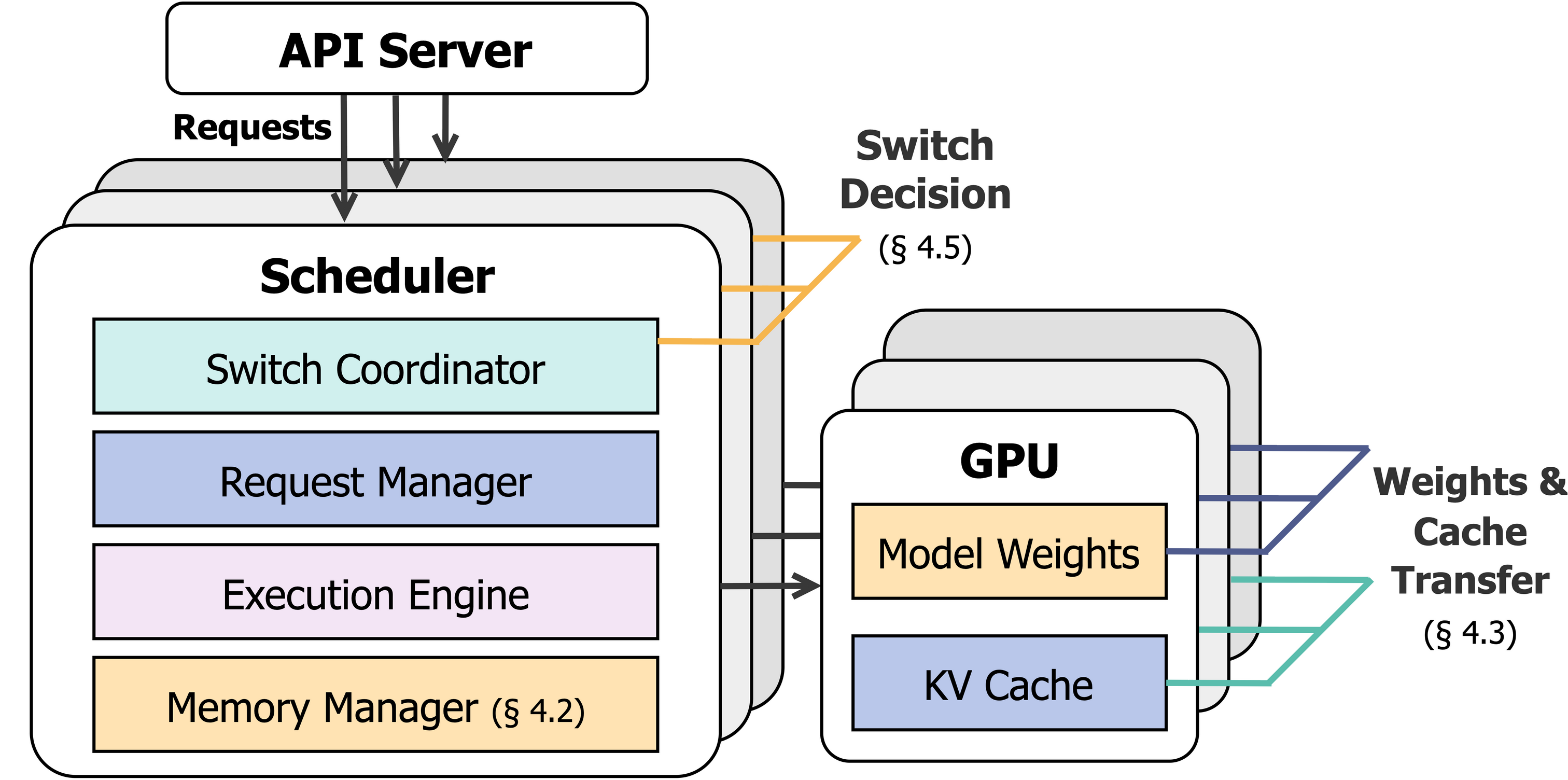
Figure 6 shows how Moebius embeds switching inside the serving runtime. A centralized API server admits requests and dispatches them to per-rank schedulers. Each scheduler contains four components: a switch coordinator that chooses the target mode, a request manager that tracks request metadata and KV-cache ownership, an execution engine that runs the active EP or TP forward path, and a memory manager that owns the rank’s GPU-resident weights, KV cache, and transfer staging buffers.
Moebius separates each switch into a control plane reconfiguration and a data-plane update. The control plane is small, so Moebius holds both the EP and TP copies resident and a switch selects prepared state instead of rebuilding it. The data plane, expert weights and KV-cache pages, is too large to replicate at model scale, so Moebius reshards the single resident copy over the interconnect.
Switches run between consecutive model forward steps. Before every step, the switch coordinator on rank 0 decides whether to switch modes according to its policy. And the decision is broadcast to other ranks. When a switch is triggered, all ranks enter the transition together: execution engines select the prepared runtime state for the target mode, request managers update request and KV-cache ownership, and memory managers move expert slices and KV pages directly between GPUs. Decoding resumes under the new layout after all ranks complete the transition.
The rest of this section describes the runtime support in dependency order: the unified memory manager fixes the storage layout (§4.2); direct-transfer kernels fuses all transfer operations (§4.3); the runtime-preservation keeps CUDA graphs and communication state valid (§4.4); and the switch policy decides when the transition is worth taking (§4.5).
4.2 Unified Memory Manager↩︎
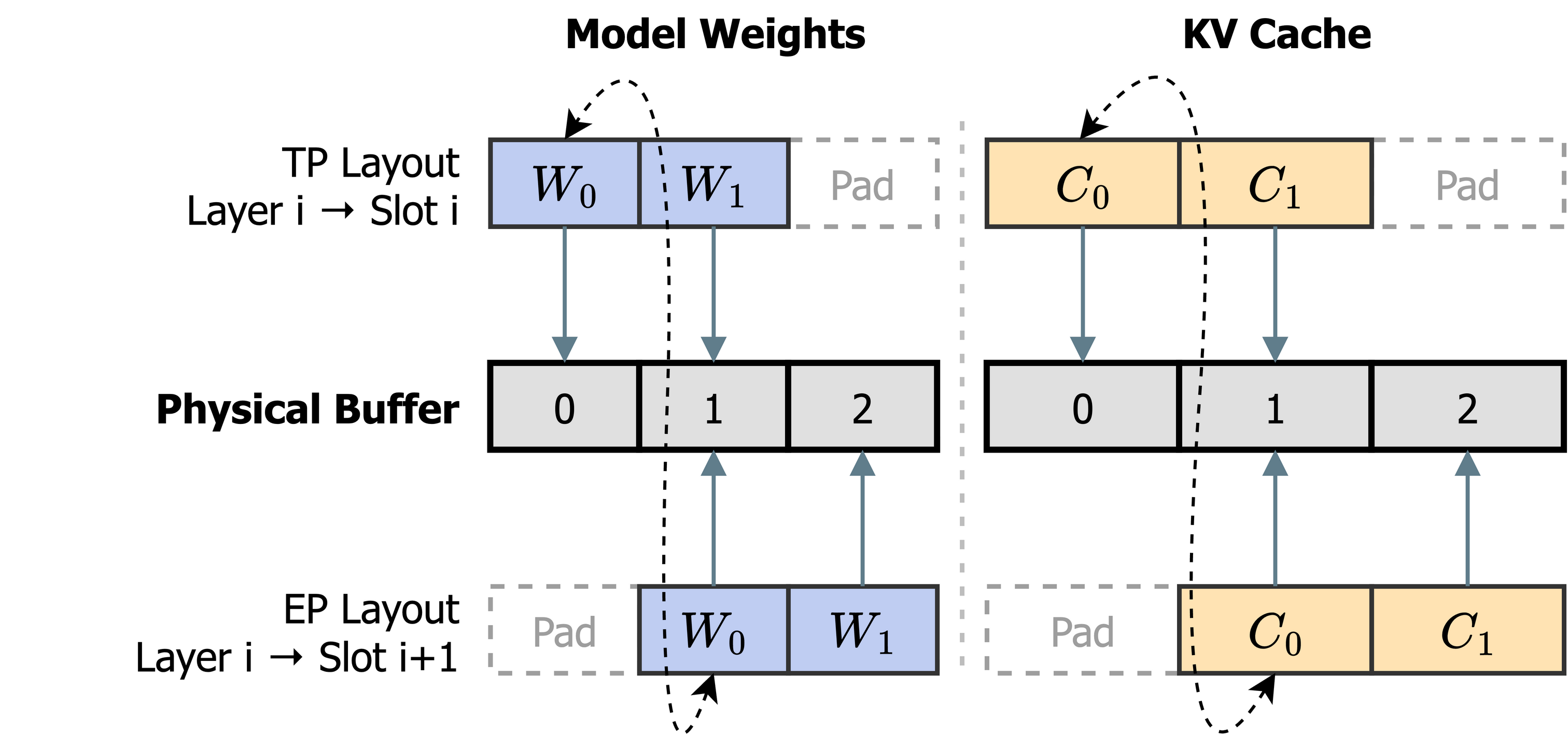
The unified memory manager (UMM) is Moebius’s GPU-memory foundation for switchable states. Instead of letting model components allocate device tensors independently, each rank allocates one large contiguous unified buffer on GPU at startup, sized by the memory fraction reserved for model weights and KV cache. UMM then serves all long-lived switch state from this buffer, including expert weights, attention weights and KV-cache pages. Each later allocation is replaced with a tensor view into a fixed region of the unified buffer, so the runtime can reason about both the physical address and the mode-specific layout of every object involved in a switch.
UMM builds this layout with slots and aliases. For expert weights, it divides the buffer into fixed-size per-layer slots and creates two sets of tensor views over them, one for TP and the other for EP. The two views expose the shape and stride that the corresponding forward path expects, but they alias the same rank-local backing buffer. To make in-place resharding safe, UMM reserves one extra slot: for \(N\) layers, TP maps layer \(i\) to slot \(i\), while EP maps layer \(i\) to slot \(i{+}1\) (Figure 7). During a switch, the transfer kernel reads from the source-mode alias and writes to the target-mode alias. The one-slot offset gives each layer separate source and destination slots, and the transfer uses the direction-specific layer order to avoid overwriting a slot before its old contents have been read. EP \(\rightarrow\) TP adopts the sequential order while TP \(\rightarrow\) EP adopts the reverse order.
This layout gives Moebius three switch-path properties. First, a switch does not allocate dynamic buffers for new weights or cache pages; target weight slots and KV-cache pages already exist inside the unified buffer. Avoiding dynamic allocation matters because new device allocations can trigger PyTorch memory garbage collection and add significant delay to the switch. Second, as the unified buffer never moves, each rank exports it once as CUDA IPC memory, and peer GPUs write target slots directly over NVLink (§4.3). Third, each mode-specific tensor keeps a fixed device-side memory address. CUDA graphs captured separately for EP and TP therefore remain valid across switches; a mode’s buffers may contain stale bytes while inactive, but the graph still refers to the same addresses when that mode becomes active again. These properties give fused transfer kernel and runtime preservation the stable storage layout they depend on.
4.3 Fused Direct Transfer Kernel↩︎
The resharding plans of §3.1 and §3.2 share a common process: gather source bytes into per-peer chunks, exchange them across ranks, and scatter the received
bytes into the target layout. The straightforward implementation maps this plan to NCCL collectives, staging each layer’s per-peer chunks in a buffer and synchronizing through an All-to-All; the KV cache adds a gather and scatter around the
exchange because paging scatters its source and destination slots.
This NCCL path is correct but slow on the switch critical path. It touches the same bytes multiple times in HBM, requires staging buffers for each active layer, and communicates through an All-to-All at every layer. Double-buffering can
pipeline staging for adjacent layers, but it needs a second staging slot and still moves data through NCCL’s internal buffers before the bytes reach their final slots.
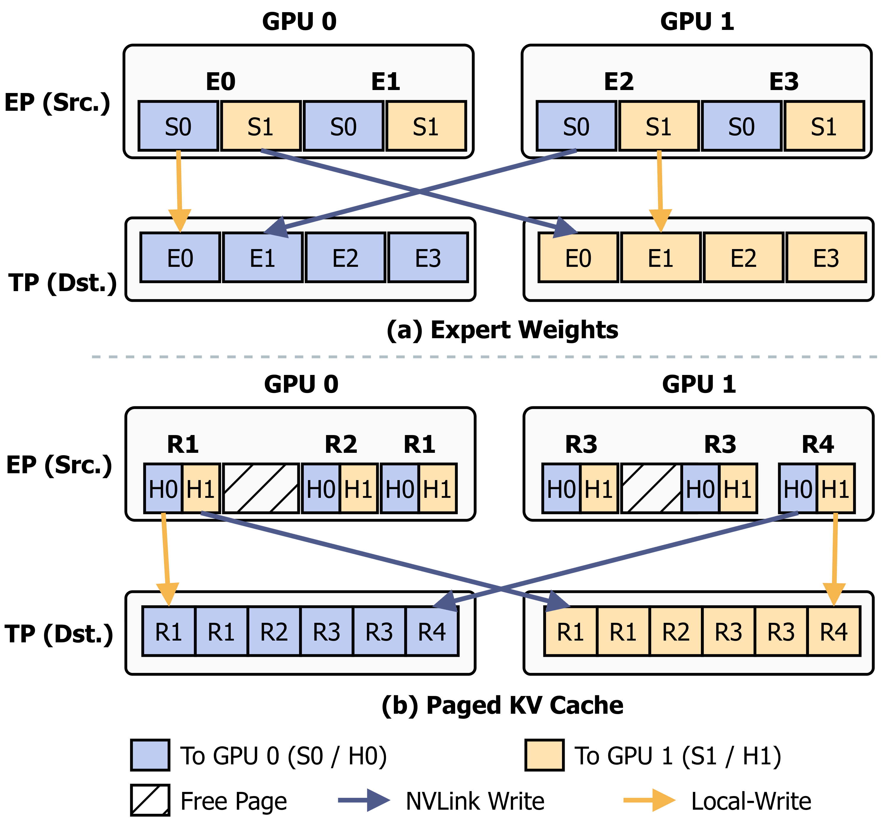
Moebius instead implements switch data movement with a direct transfer CUDA kernel library. UMM gives each rank a fixed backing-buffer address, so each rank exports that buffer once as a CUDA IPC handle and maps its peers’ buffers into its own address space. The library provides separate kernels for the two data-plane objects that a switch moves (Figure 8). Expert-weight kernels operate on dense expert slices: each kernel reads from the source-mode alias and writes the slice into the peer’s target-mode slot over NVLink. KV-cache kernels operate on paged cache metadata: they read the page tables for live requests, read scattered source blocks through those tables, and write the corresponding target pages directly into peer buffers.
Both kernel families have the same switch-path benefit. They collapse staging, data exchange, and scatter into a direct write to the final destination, so the switch does not materialize per-peer chunks in intermediate buffers or communicate through a
per-layer All-to-All. The required source and destination regions already exist inside UMM, so the kernels also avoid dynamic allocation for new weights or cache pages during the switch.
Table 1 summarizes the resulting data movement. NCCL stages every element through HBM: two reads and one write for weights, and an extra read and write for the cache because scattered pages are first gathered into a contiguous buffer. The fused direct transfer kernel makes a single pass for both objects: one HBM read, and one NVLink store into the peer’s slot. It allocates no staging buffer; instead, it utilizes the extra UMM destination slot already needed for safe in-place resharding. Thus our transfer kernel uses one extra slot like naive NCCL, while overlap’s double buffering costs two. In every method, the \(1/P\) of each object whose destination is the sending rank itself is a local HBM write rather than an interconnect transfer; Table 1 folds this local write into the NVLink column for simplicity.
| Method | Buffer | HBM | NVLink | |
|---|---|---|---|---|
| Weights | Naive | \(S\) | 2 + 1 | 1 |
| Overlap | \(2S\) | 2 + 1 | 1 | |
| Direct | \(S\) | 1 + 0 | 1 | |
| Cache | Naive | \(2S\) | 3 + 2 | 1 |
| Overlap | \(4S\) | 3 + 2 | 1 | |
| Direct | \(S\) | 1 + 0 | 1 |
The KV-cache kernels differ from the weight kernels in how they construct this final-destination write. Expert-weight traffic is dense and balanced by layer, but KV traffic is fine-grained and depends on the live request set where different ranks may
own different numbers of tokens, and sequence lengths make the All-to-All volume imbalanced. Moebius therefore builds page-indexed work descriptors from the current request metadata, as shown in Figure 8,
and launches KV kernels over those descriptors. The kernel still performs the same direct write as the weight path, but it derives its source and destination addresses from the irregular cache layout produced by paged attention.
4.4 Runtime Preserving↩︎
A switch changes the data layout, but the serving runtime also depends on mode-specific execution state. CUDA graphs, communication groups, EP communication buffers [17]–[19], and attention-backend metadata [30], [31] must match the active EP or TP forward path and are expensive to reconstruct, yet together they are small enough to keep resident in both modes. Moebius therefore builds both runtime-state bundles at startup and switches between prepared copies at an iteration boundary.
CUDA graphs impose the strongest constraint because graph replay embeds device memory addresses and forces every input tensor to stay at a fixed address. EP and TP use different forward paths, so Moebius captures one graph set per mode. Both graph sets reference UMM-managed mode-specific tensors. Across switches, those tensors keep the same addresses; while a mode is inactive, its buffers may contain stale bytes, but the next switch writes the target-mode data back into those same buffers before the graph is replayed. A switch therefore changes buffer contents, not graph addresses. During startup, Moebius captures both graph sets against their real layouts, using a weight-only warmup switch to enter the alternate mode while no request is active.
The same resident-state rule applies to communication and attention state. Moebius keeps per-mode communication and attention metadata buffers resident. When the first rank commits a switch, each rank flips the active graph set, communication state, and attention metadata together, and the request manager hands request ownership to the target layout in the same step (§3.2). The resumed decode step then observes a consistent target-mode runtime without recapturing graphs or rebuilding runtime state.
4.5 Switch Policy↩︎
Rank 0 runs the switch coordinator, which decides when the efficiency gained by changing modes outweighs the switch cost. Moebius uses the global in-flight request count as the control signal, because it tracks the per-iteration work that determines the TP–EP crossover. The coordinator samples this count once per decode iteration, after the current step completes and before the next step begins, so the policy never interrupts a forward pass.
The policy is asymmetric. When Moebius runs in TP, a sudden load increase can make TP throughput-bound, so the coordinator switches to EP as soon as the latest count exceeds a high threshold \(T_h\). When Moebius runs in EP, a temporary dip below the crossover is less urgent, since switching too early can cause oscillation. The coordinator therefore switches back to TP only when the mean count over the last \(W\) iterations falls below a low threshold \(T_\ell\). The band \(T_\ell \le T_h\) provides hysteresis, and a cooldown \(C\) after every switch bounds the maximum switching rate.
Moebius sets the thresholds after startup calibration. Once CUDA graphs have been captured for both modes, the coordinator probes EP and TP decode cost over a small set of batch sizes and chooses the crossover as the initial threshold. Interactive serving uses a wider band and a longer averaging window, making EP sticky during short load dips. Synchronous rollout uses \(T_\ell=T_h\) and \(W=1\), because the workload arrives as one burst and then drains monotonically.
Before committing a decision, Moebius checks that the target mode has enough KV capacity for the current live requests. This matters when the model has fewer KV heads than ranks: TP replicates each head across ranks, reducing aggregate KV capacity compared with EP (Qwen3-235B has four KV heads on eight ranks). If the target mode cannot fit the current request and token set, rank 0 cancels the switch and retries after the cooldown. Otherwise, it broadcasts the target mode, and all ranks transition together at the next iteration boundary.
5 Implementation↩︎
Moebius is built on SGLang v0.5.5 [6], and its mechanism is a self-contained module of roughly 7,400 lines: the unified memory manager, fused direct-transfer kernels, and switch coordinator. Integrating it into the serving engine modifies only about 200 lines of existing SGLang code, adding new code paths rather than rewriting existing ones. An operator enables Moebius and sets its policy entirely through launch arguments: the high threshold, hysteresis band, window, and cooldown are command-line parameters, with the crossover auto-calibrated at startup (§4.5). Running it needs no change to model weights, the request API, or the surrounding training and serving stack, and the switch coordinator runs on rank 0 inside the existing engine process, so there is no separate controller to provision or monitor.
6 Evaluation↩︎
Our evaluation answers five questions. (1) Does adaptive EP\(\leftrightarrow\)TP switching beat the better static layout when load crosses the crossover mid-run? (2) Does the win hold for both online serving and batch generation? (3) What does a single switch cost? (4) What does preserving CUDA graphs across switches save? (5) How much memory does keeping both layouts resident add? We answer (1) and (2) on two workloads that cross the crossover from opposite directions, bursty serving (§6.2) and RL rollout (§6.3), then isolate the switch (§6.4), the CUDA-graph cost it avoids (§6.5), and the memory of holding both layouts (§6.6).
6.1 Experimental Setup↩︎
Hardware and model. We evaluate Moebius on a single node of 8 NVIDIA H200 GPUs (141 GB HBM each), fully connected over NVLink, serving the instruction-tuned Qwen3-235B-A22B model in BF16 (235B parameters, 94 layers, 64 query / 4 KV heads).
Systems. We compare three SGLang deployments (§5) that differ only in parallelism layout. The two static layouts are the production-grade configurations an operator would actually deploy, and bracket the EP\(\leftrightarrow\)TP tradeoff:
TP runs 8-way tensor parallelism for both attention and the MoE experts.
EP runs data-parallel attention with 8-way expert parallelism, using DeepEP for expert dispatch and combine.
Moebius runs both layouts and switches between them at runtime (§4.5): it enters EP when the latest in-flight count exceeds a high threshold \(T_h\), and returns to TP when the count averaged over a window of \(W\) iterations falls below a low threshold \(T_\ell\), with a cooldown \(C\) between switches.
Configuration. All three systems share the same configuration: radix cache disabled, overlap scheduling enabled, a 2,048-request concurrency cap, 0.85 static memory fraction, and CUDA-graph enabled. The prefill token cap follows the active layout, sized to avoid OOM under each layout: 8,192 tokens in TP and 4,096 tokens per rank in EP.
Moebius’s switch policy (§4.5) fixes \(T_h=256\) and cooldown \(C=5\,\)s, widening the band and window for interactive serving (\(T_\ell=0.8\,T_h\), \(W=8\)) and collapsing them for rollout (\(T_\ell=T_h\), \(W=1\)). All runs report output throughput (decode tokens/s) and sample the active parallelism mode and running-request count at 1 Hz. Workload-specific metrics are defined per subsection.
6.2 Bursty Online Serving↩︎
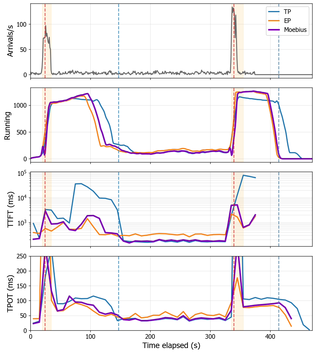
Online request rates rise and fall, so a single deployment crosses the EP\(\leftrightarrow\)TP operating point repeatedly within one run and pays in whichever regime it is not built for. Moebius instead tracks the favorable mode as the rate moves.
Workload. We replay a 3,107-request arrival trace generated by the vLLM bursty workload generator [7], spanning 375 s and identical across all three systems. Two short bursts (peak 80 and 120 requests/s) bracket a 300 s quiet period at 1–5 requests/s. Prompts are ShareGPT samples of 300–700 tokens with outputs from \(U(800, 1200)\) tokens. The bursts drive concurrency well above \(T_h\), and the quiet period drops it back below. Moebius uses the interactive setting, so it retreats to TP only under sustained low load. It switches four times over the trace, into EP at each burst onset and back to TP after each burst drains. We report mean time-to-first-token (TTFT) over arrivals in 10 s bins and mean time-per-output-token (TPOT) over tokens emitted in the same bins.

Each static layout pays in one regime. Static layouts trade strengths on opposite ends of the trace (Figure 9). TP’s decode trails EP under
burst load. Its queue outruns it and mean TTFT reaches 9.9 s, roughly five times EP’s 2.0 s. EP absorbs both bursts but pays in the quiet stretch, where All-to-All dispatch overhead
lifts TPOT to 52 ms against TP’s 37 ms, a 40% gap that compounds across every decoded token.
Moebius tracks the favorable layout. Running EP through each burst and TP through the quiet period, Moebius stays on the side that is winning at each point of the trace (Figure 9). Its quiet-period TPOT tracks TP and stays well below EP. Its burst TTFT peaks at 3.1 s, three times below TP and close to EP. On the tail, its p99 TTFT holds at 6.0 s and 1.9 s across the two bursts, far below static TP’s 90 s burst-onset collapse, so the sub-second switch pause never drives the tail. The residual gap to EP reflects the early-burst TTFT Moebius accrues before its TP\(\to\)EP switch completes (§6.4), the cost of starting each burst in TP.
6.3 Rollout Workloads↩︎
Reinforcement-learning post-training, such as GRPO [9] and DAPO [10], interleaves policy updates with rollout steps. Each step is itself a serving workload: it submits a large batch of prompts and generates every one to completion before the next weights update. Because output lengths are heavy-tailed, the batch starts large and decays toward a long tail of still-decoding requests. A rollout step therefore crosses the EP\(\leftrightarrow\)TP operating point within a single step: the large initial batch favors EP, the small late-stage batch favors TP. Any fixed deployment commits to one side of this tradeoff for the entire run. Moebius instead preserves in-flight requests and changes the parallelism layout as the active batch shrinks.
Workload. We use the DeepMath math-reasoning benchmark [32] on Qwen3-235B: each rollout step submits a batch of \(N=2048\) prompts and decodes every one to a 32,768-token cap. This is representative of production RL, which runs steps of one to eight thousand prompts under 16k–32k-token caps [10], [22]–[25]. Pooled over the nine steps (18,432 requests), inputs are short and clustered (median 120 tokens, max 1,352). Outputs are long and heavy-tailed (median 1,510 tokens, p99 10,386), with the longest reasoning chains running to the 32k cap (Figure 14). This asymmetry makes the step decode-dominated and gives the active batch its slow decay: the median request finishes early, while a few long outputs keep decoding an order of magnitude longer and drag the in-flight count down a long tail.
Methodology. To hold the decode work identical across systems, we capture each request’s output length once under EP’s natural generation, then replay those exact lengths under TP and Moebius. Every system therefore decodes the same number of tokens for every request, isolating system performance from layout-induced differences in output length. EP’s capture run serves as its own datapoint. Steps vary in prompt mix and so in output-tail shape, so we evaluate nine steps spanning light to heavy tails, holding the policy fixed so the only variation is the workload. Because the active batch only shrinks, Moebius uses the rollout setting: it starts in EP and switches once to TP when the batch drains below \(T_h\). We report end-to-end completion time.
The win is phase-matching, not a per-token speedup. Figure 10 shows Moebius fastest at all nine steps, beating the better static layout by 1.16–1.25\(\times\) (mean 1.22\(\times\)) and the worse by up to 1.31\(\times\). The more telling result is which static layout is better: EP wins most steps on burst throughput, but on the heaviest-tailed steps, where the rollout lingers in the small-batch tail, TP pulls ahead, so which layout wins depends on the step’s prompt mix and is not known until the step has run. The “better static layout” that Moebius is compared against is therefore an oracle that picks the faster of TP and EP per step with foreknowledge, a choice no operator can deploy, yet Moebius beats even this oracle because its gain comes from switching within a step rather than committing to one layout for the whole step. The split bars expose why Moebius beats both: within every step EP clears the burst phase faster while TP decodes the long tail faster, and Moebius runs the burst in EP and the tail in TP, tracking the faster layout in both phases.
End-to-end projection. The per-step speedup translates to end-to-end training time through the rollout fraction and the framework’s overlap scheme (§2.2). For synchronous on-policy training at a 65–85% rollout fraction, Amdahl’s law projects our 1.16–1.25\(\times\) per-step gain to 1.10–1.20\(\times\) end-to-end, and rollout-bound asynchronous schemes pass it through more directly (Appendix 11).
6.4 Switch Cost and Optimizations↩︎
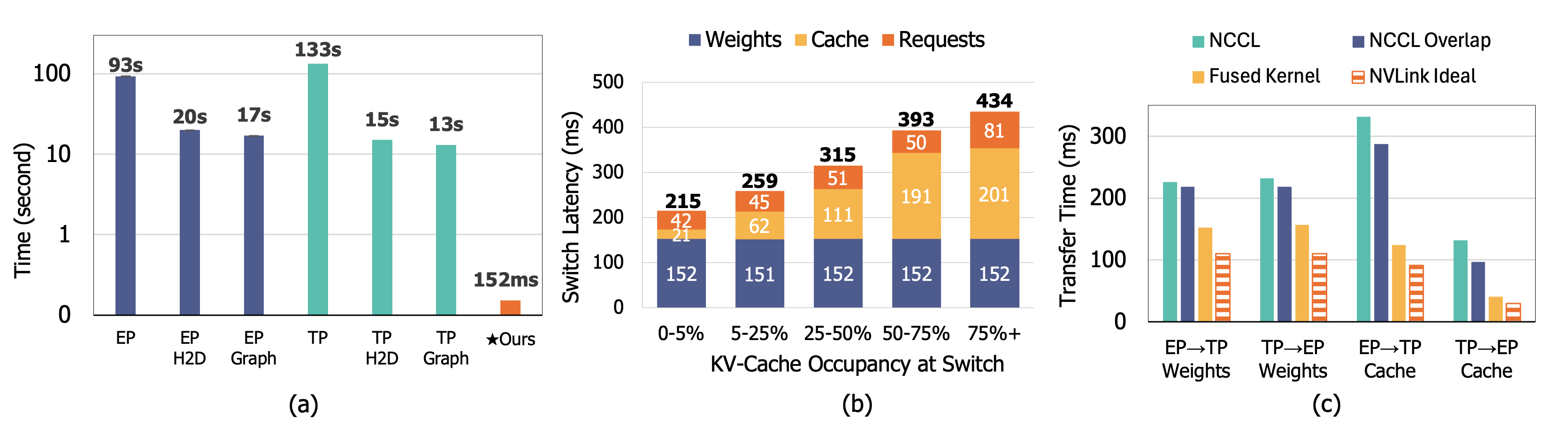
A switch redistributes three pieces of resident state: expert weights, the paged KV cache, and request ownership. Figure 11 isolates its cost three ways. Panel (a) sets the bar against reconfiguration strawmen that drain the batch and rebuild the target layout, panel (b) decomposes a production EP\(\to\)TP switch by phase across KV-cache occupancy, and panel (c) pits the fused-kernel transfer against NCCL collectives over both components and directions.
Switching without rebuilding wins by orders of magnitude. Panel (a) drains the in-flight batch and compares Moebius’s bidirectional switch against three rebuild strawmen (Figure 11 (a)). The strawmen strip one cost at a time: restart pays cold model load and graph recapture, host-memory weight loading drops the disk load, and reusing Moebius’s fused transfer leaves only recapture, needed because the rebuilt buffers land at fresh addresses. Every rung still costs seconds to minutes. By transferring into pinned addresses and keeping both graph sets resident, Moebius avoids reload and recapture alike, switching in 152 ms, orders of magnitude faster (§6.5).
The cheap switch is what makes within-episode adaptivity viable. A switch is worth taking only when it costs less than the work it saves. On the 375 s bursty trace Moebius switches four times. At the restart strawman’s 93–133 s per switch, or even the host-reload and graph-recapture variants’ 13–20 s, the switch cost alone would dwarf the trace and make naive adaptivity net-negative. Beyond cost, every rebuild path must drain the in-flight batch before it can reshard. Applying one during serving would stall or drop live requests, which production serving cannot accept regardless of latency. Moebius’s switch sits two to three orders of magnitude below this bar while retaining the ongoing requests, which is what lets it follow the favorable layout within an episode rather than only across deployments. We therefore characterize these rebuild paths as switch-cost bounds (Figure 11 (a)) rather than running them as end-to-end baselines. A full-workload comparison would only restate the loss which their per-switch cost and forced draining already guarantee.
A switch is a fixed weight floor plus a load-dependent KV term. We mine 16 EP\(\to\)TP switches from our rollout and serving runs and split each into its three phases, binning by KV-cache occupancy (Figure 11 (b)). Weight transfer is a fixed cost floor, the same reshard panel (a) measures with the batch drained. Only the KV phase grows monotonically with occupancy, and it sets the gap between a light and a heavy switch. Request redistribution tracks the in-flight request count rather than per-request cache footprint, so it stays flat. Even with the cache full the total stays under half a second, and its spread comes almost entirely from KV volume.
The win extends to the KV cache and the reverse direction. Across KV-cache transfer and the TP\(\to\)EP direction (Figure 11 (c)), the fused kernel sustains above 70% of NVLink peak on every bar, reshards expert weights 1.49\(\times\) faster than NCCL in both directions, and beats it by over 2\(\times\) on the cache. Even the 70% floor sits closer to the hardware limit than it appears. Fusing the layout transform into the copy keeps the transfer on the SMs, which in our measurements top out near 77% of peak rather than the roughly 90% a dedicated copy engine reaches, a ceiling unavailable here because a copy engine cannot reshard on the fly. Against that 77% attainable ceiling, holding above 70% of peak already puts the fused kernel over 90% efficiency, so the reshard is effectively saturating the SM transfer path with little headroom left to recover. Overlapping the collectives across CUDA streams does not close the gap, because on flat NVL8 every GPU pair shares one fabric, leaving the collectives bandwidth-bound so pipelining pays off only on hierarchical interconnects. Even EP\(\to\)TP, the costlier direction because TP replicates each KV head across two ranks and so doubles the per-rank bytes, stays well below NCCL, so KV transfer is not the bottleneck.
6.5 Cost of Preserving CUDA Graphs↩︎
Moebius captures both the EP and TP graph sets at startup and keeps both resident, so a switch swaps the active graph pointer in under a millisecond rather than rebuilding any graph (§4.4). This avoids two costs at once: the per-switch recapture stall already charged to the strawmen in §6.4, and a per-token tax from decoding eagerly with no graph at all. We measure that per-token tax on the same Qwen3-235B, 8\(\times\)H200 configuration.

Eager decoding taxes every step. Without graphs, each step issues every layer’s kernel launches individually instead of replaying them in one graph launch (Figure 12). The host overhead hurts most where compute is smallest, up to \(6.95\times\) at the low batch sizes Moebius runs in TP, and shrinks but never disappears as the batch grows. That worst case falls in low-concurrency TP, exactly the regime Moebius enters TP to serve, so preserving graphs is what makes that mode viable. Eager decoding is also unpredictable, with GC and launch-queue stalls spiking occasional steps well above the median.
Holding both graph sets resident is cheap. Each mode caps capture at a per-rank batch of 256 and so holds only 36 graphs, small enough to keep both sets resident (§6.6). The cap is safe because Moebius enters EP rather than decoding in TP above the \(T_h=256\) crossover, and EP’s data-parallel attention keeps each rank at or below 256 even at full concurrency. Paying this capture once at startup, rather than at every switch, is what turns the per-switch recapture stall of §6.4 into a sub-millisecond pointer swap.
6.6 Memory Footprint↩︎
Moebius keeps both the EP and TP layouts resident, so a natural concern is that it doubles the memory of a single-layout server. It does not. We measure per-GPU memory at rest, after weight load, KV-cache allocation, and CUDA-graph capture but before any request, on the same 8\(\times\)H200, Qwen3-235B, 0.85 memory-fraction configuration as above. This static snapshot is the whole story: at switch time and during serving Moebius reuses pre-allocated buffers rather than materializing new tensors. Figure 13 splits each footprint into model weights, KV cache, Moebius’s dual-mode buffer, and runtime state, the last detailed in Appendix 12.
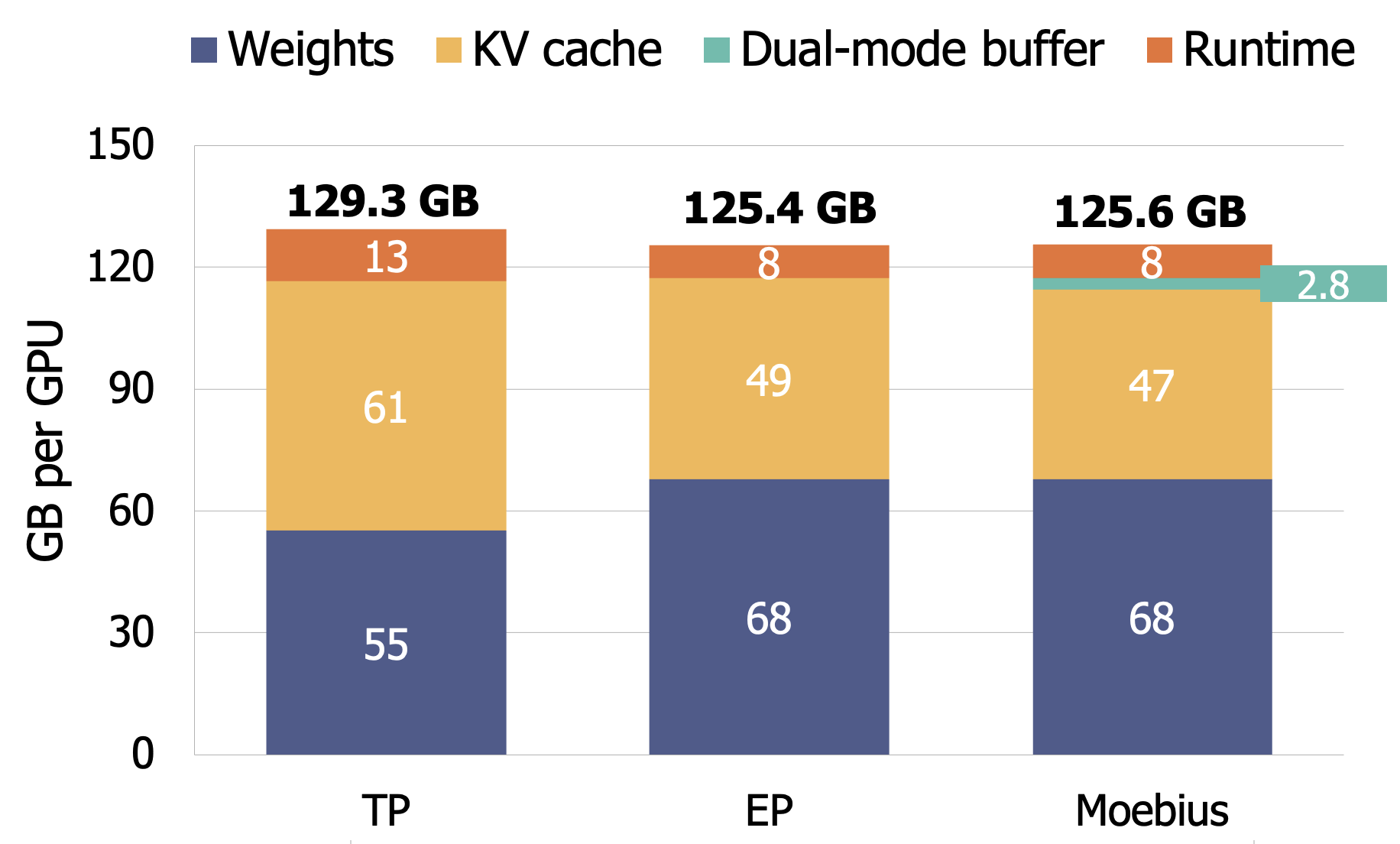
Two resident layouts, one memory budget. Although Moebius holds two CUDA-graph sets and both attention layouts, it fits within EP’s budget: within 0.2 GB of EP and 3.7 GB below TP (Figure 13). The heavy state is shared, not duplicated: its weights are identical to EP’s, and the MoE experts, EP communication buffer, and NCCL communicators are allocated once and reused in both layouts. Moebius and EP carry 12.7 GB more weight per GPU than TP only because data-parallel attention replicates the attention stack on every GPU, a cost of EP rather than the price of holding two layouts. Its one genuine overhead is a 2.8 GB dual-mode buffer: it holds the TP-mode attention shards alongside the full EP copies so a switch stays a pointer swap, plus a spare physical layer that stages the per-layer transfer (Appendix 12). Because these bytes sit inside the weight allocation, Moebius funds them by forgoing 2.8 GB of KV cache (\(+2.4\%\) per GPU) rather than adding memory on top. Even charged the full buffer it stays below TP, since it sizes its TP-mode graphs and workspaces for a batch of 256 rather than TP’s full 2,048.
7 Related Work↩︎
Runtime parallelism switching. Prior runtime switching targets dense serving or stays within training, never a live MoE EP\(\leftrightarrow\)TP serving switch. SpotServe [33], Amoeba [14], Flying Serving [15], and Shift Parallelism [13] switch dense serving among data, tensor, and sequence parallelism, while HotSPa [34] and Tutel [35] switch at training-step boundaries. Moebius reshards its memory-dominant experts without replica, and repartitions the KV cache for in-flight requests.
Serving and execution for MoE. Among MoE systems, HAP [36] chooses hybrid layouts offline with no online transitions, while the rest optimize a single fixed layout: DeepSpeed-MoE [37] and DeepSpeed-Inference [38] scale expert inference, Lina [39] targets communication cost. The fused EP communication kernels [17]–[19] improve token dispatch, and hybrid mappings [40] still commit to one deployment layout. Moebius is orthogonal: it switches layouts as load changes and reuses these kernels inside each mode. It also preserves the standard serving stack across a switch, building on continuous batching (Orca [41]), paged KV cache (vLLM [7]), SGLang’s EP and TP forward paths [6], and FlashAttention [31] and FlashInfer [30] kernels, with a unified memory manager that keeps these CUDA graphs valid after a reshard (§4.2).
Serving for RL rollout. RL post-training turns rollout into a serving workload. HybridFlow [12] and OpenRLHF [11] orchestrate rollout and training, GRPO [9] and DAPO [10] defines our rollout workload, and StreamRL [27] and AReaL [28] hide rollout cost through disaggregation or asynchrony. Rollpacker [22] and TLT [42] targets eliminating and accelerating the long tail problem. Moebius is orthognal to them and can be integrated in the rollout engine to collectively improve rollout efficiency.
8 Discussion↩︎
Generality of the mechanism. Moebius separates a model-agnostic control path from architecture-specific resharding that depends only on the expert count \(E\), rank count \(P\), hidden size \(H\), and intermediate size \(I\). Grouped- and multi-head attention, finer-grained or shared experts, and multi-head latent attention therefore fit by changing only how a tensor is sharded, not the control path. Those speedups are specific to our model and hardware.
Capacity-aware switching is safe by construction. When KV heads are fewer than ranks, TP holds less KV cache, and on eight ranks Qwen3-235B’s four KV heads halve TP capacity. Moebius switches to TP only when the live KV fits and otherwise stays in EP (§4.5), so a canceled switch forgoes a latency gain but never admits an infeasible layout, leaving Moebius bounded below by the better feasible static layout.
Scope and future work. The framework is topology- independent, but the direct-transfer kernel targets a single NVLink domain, where it reshards 1.49\(\times\) faster than an NCCL collective (§6.4). Across nodes the switch falls back to a collective while still keeping one resident weight copy, preserving CUDA graphs, and migrating live requests, and a direct path over RDMA remains future work. Our rollout numbers also measure the generation engine alone, so coupling Moebius with a full RL system that spans generation, policy updates, and scheduling, to turn per-step speedups into end-to-end training gains, is likewise left to future work.
9 Conclusion↩︎
MoE serving shows a TP–EP performance crossover where production workloads cross at runtime. TP decodes small batches with lower latency and EP sustains throughput with large batches. Moebius makes the layout reconfigurable by treating an EP\(\leftrightarrow\)TP switch as a change of data ownership rather than semantics, resharding resident expert weights and KV cache over the interconnect without a second replica while in-flight requests and captured CUDA graphs survive the switch. On 8\(\times\)H200 GPUs serving Qwen3-235B, Moebius is fastest on every RL-rollout step, and completes each switch in 215–434 ms at 2.4% memory overhead, beating the better static layout by 1.16–1.25\(\times\).
10 Rollout Workload Distribution↩︎
Figure 14 plots the input and output token-length CDFs pooled over the nine DeepMath rollout steps (18,432 requests). The two are sharply asymmetric: inputs are short and tightly clustered, while outputs are long and heavy-tailed, running out to the 32k decode cap. This output tail is what makes a rollout step’s active batch decay slowly, the property the rollout evaluation (§6.3) exploits.

11 End-to-End Training Projection↩︎
Our per-step rollout speedup carries to end-to-end training time differently depending on how the RL framework overlaps generation with policy updates (§2.2). Synchronous on-policy training waits for the full rollout step before each update [11], [12], [26], so by Amdahl’s law a per-step speedup \(s\) over a rollout fraction \(f\) gives \(1/((1{-}f)+f/s)\) end-to-end, and reported fractions of 65–85% [22], [42] turn our 1.16–1.25\(\times\) into 1.10–1.20\(\times\). One-step-stale overlap is rollout-bound, so the gain passes through nearly one-to-one [27], [28], while partial-rollout [28], [29] and trajectory-level asynchronous [24] schemes reshape the per-step workload and need a real integrated run to quantify. We report the per-step speedup as our measured result and treat these end-to-end figures as projections.
12 Runtime Memory Breakdown↩︎
Table 2 details the per-GPU runtime state of Figure 13, the footprint outside weights, KV cache, and the dual-mode buffer. The 2.8 GB dual-mode buffer itself divides into 1.7 GB of
TP-mode qkv_proj and o_proj shards held alongside the full EP copies and 1.1 GB for one spare physical layer that stages the per-layer transfer. TP’s larger activation workspaces and CUDA graphs
follow from sizing for its full 2,048-request batch, where Moebius and EP size for a per-rank batch of 256. The 12.7 GB weight gap between data-parallel attention (Moebius, EP) and sharded
attention (TP) comes from the attention projections. Qwen3-235B’s attention uses 64 heads of dimension 128, so its q/k/v/o projections total roughly 13 GB in BF16 across its 94 layers. TP holds
one-eighth per GPU, EP a full copy, with the per-rank embedding and LM head making up the small remainder. TP’s smaller weight footprint leaves it the most room for KV cache, but the extra
capacity buys little throughput, since TP’s decode is bound by compute and communication rather than concurrency.
| Component | TP | EP | |
|---|---|---|---|
| Activation workspaces | 7.6 | 3.1 | 3.0 |
| CUDA graphs | 1.8 | 0.8 | 0.9 |
| EP infra (DeepEP + NVSHMEM) | — | 2.2 | 2.2 |
| NCCL communicators | 0.6 | 0.6 | 0.6 |
| Other (NCCL VMM, cuBLAS, IPC) | 2.9 | 1.4 | 1.7 |
| Total runtime | 12.7 | 8.1 | 8.3 |