SharQ: Bridging Activation Sparsity and FP4 Quantization for LLM Inference
June 25, 2026
Abstract
Low-bit floating-point formats and semi-structured sparsity are increasingly supported by modern accelerators, yet combining them for LLM activation compression remains challenging: activations contain input-dependent outliers that dominate block scales in FP4 quantization, and directly applying N:M sparsity masks discards moderate values, coupling sparsification loss with quantization error. We introduce SharQ, a training-free inference method that bridges activation sparsity and FP4 quantization through an online sparse–dense decomposition. For each activation tensor, SharQ generates an input-adaptive N:M mask to extract an outlier-dominated sparse backbone, quantizes it to FP4, and defines a dense residual relative to the quantized sparse backbone rather than the unquantized sparse values. A sparse FP4 GEMM processes the backbone while a dense FP4 GEMM compensates for both mask-induced activation loss and sparse-path quantization error. The two paths share a single FP4 weight payload with path-specific scale views, and a fused preparation kernel absorbs mask generation, residual construction, and layer normalization into one operator. SharQ requires no calibration data, retraining, or model-specific tuning. Evaluated on Llama-3.1-8B, Qwen2.5-7B, Qwen3-30B-A3B, and Qwen3-VL-8B, SharQ recovers 43–63% of the NVFP4-to-FP16 accuracy gap across language and vision-language tasks, and generalizes across NVFP4, HiF4, and MXFP4 formats. On an RTX 5090, SharQ delivers 2.2–2.4\(\times\) latency reduction over FP16 and 1.2–1.4\(\times\) throughput improvement over FP8 in language model serving, and up to 1.58\(\times\) speedup on Wan2.2-T2V-A14B video generation when combined with SageAttention. Our code is available at https://github.com/actypedef/SharQ.
1 Introduction↩︎
Large language model inference is dominated by linear layers. As model size and serving demand continue to grow, reducing the cost of matrix multiplication has become a central systems problem. Low-bit floating-point formats and semi-structured sparsity are two increasingly practical directions, because they are no longer only algorithmic compression techniques but are also exposed as hardware execution paths. Block-scaled FP4 formats such as NVFP4, MXFP4, and HiF4 improve compute density while retaining a floating-point-like dynamic range, and N:M semi-structured sparsity enables sparse matrix multiplication on modern Tensor Cores [1]–[5]. These trends suggest an appealing target for LLM inference: combine FP4 quantization with hardware-supported sparse computation.
However, applying FP4 quantization to activations remains difficult. Compared with weights, activations are input-dependent and often contain a small number of large-magnitude outliers [6]–[8]. Since block-scaled FP4 quantization chooses local scales from the largest values in each block, these outliers can dominate the scale and reduce the effective precision available to ordinary activation values. Prior work on LLM quantization, including LLM.int8(), SmoothQuant, AWQ, GPTQ, OmniQuant, QuaRot, and SpinQuant, has shown from different angles that outliers and activation distributions are central obstacles for low-bit inference [6], [9]–[14]. Mixed-precision or outlier-aware paths can reduce this error, but they often introduce extra storage, irregular data movement, or additional kernels that are less attractive for an FP4 execution pipeline.
Activation sparsity offers a tempting alternative. In many LLM layers, the largest activation values are sparse and carry a disproportionate part of the output contribution. This suggests that one might route these large values to a sparse path and exploit N:M sparse Tensor Core instructions. Yet direct activation sparsification is too lossy in a training-free setting. Unlike weight sparsity methods such as SparseGPT and Wanda [15], [16], where the mask can be optimized or calibrated offline, an activation mask must be produced online for the current input. Moreover, inference-oriented activation sparsity methods such as DejaVu and PowerInfer [17], [18] often rely on coarse-grained prediction or routing, while fine-grained N:M activation masks must satisfy strict hardware patterns and be generated cheaply on the critical path. If the sparse path simply keeps the largest values and drops the rest, many moderate activation values are lost, leading to substantial accuracy degradation.
The difficulty is therefore not only how to combine sparsity with quantization, but how to define their roles. In a sparse FP4 path, sparsification changes the local value distribution before quantization, and the FP4 scale is then selected from this changed distribution. The error is not the sum of an independent sparsification error and an independent quantization error: the two are coupled. A useful design should preserve the hardware benefit of sparse FP4 computation while retaining the activation information that does not fit into the sparse representation.
We introduce SharQ, a training-free inference method that bridges activation sparsity and FP4 quantization through an online sparse–dense decomposition. SharQ does not treat activation decomposition itself as the novelty. Instead, it makes the decomposition input-adaptive, hardware-valid, and quantization-aware. For each activation, SharQ generates an online N:M mask that extracts an outlier-dominated sparse backbone. This backbone is quantized and executed by a sparse FP4 GEMM. SharQ then defines a dense residual relative to the quantized sparse backbone, rather than relative to the unquantized sparse values. As a result, the residual contains both the values outside the sparse mask and the quantization error introduced by the sparse FP4 path. A dense FP4 GEMM then accumulates this residual contribution into the sparse output. Figure 1 provides an overview of this pipeline.
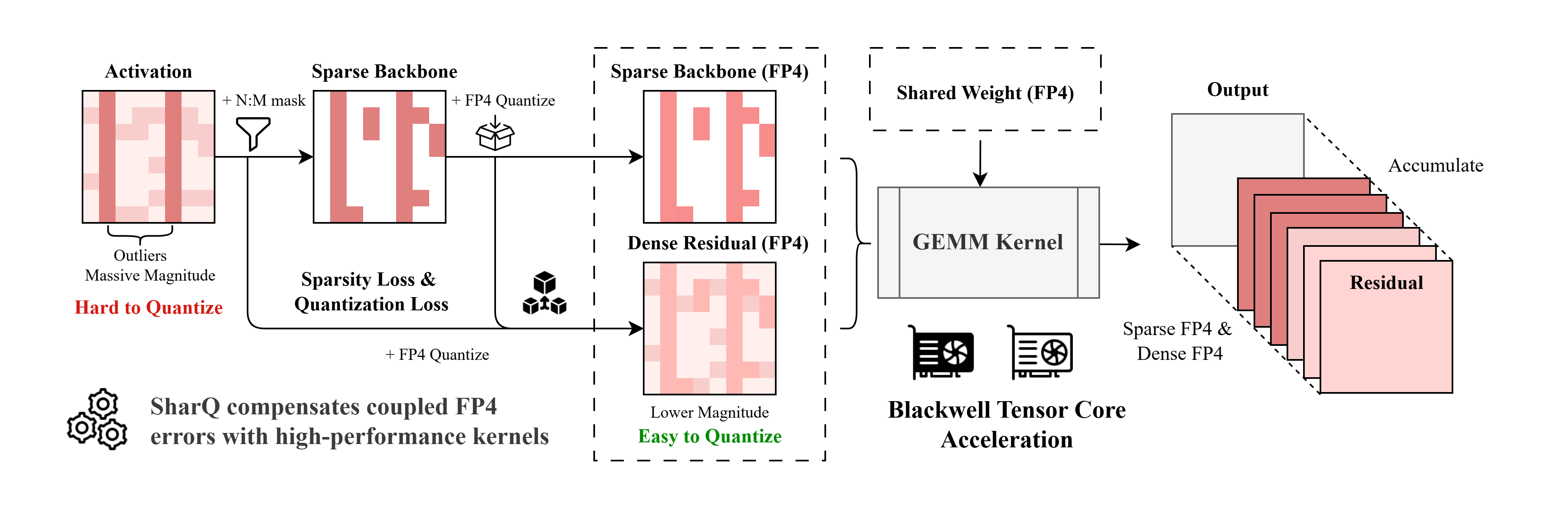
This design has two practical consequences. First, the sparse mask is determined from the current activation, so SharQ does not require calibration data, finetuning, or a learned offline mask. This helps explain why the same mechanism works across dense decoder-only models, mixture-of-experts models, video generation models such as Wan2.2 text-to-video [19], and different FP4 formats. Second, SharQ is designed around real kernel constraints: mask selection, sparse input compression, and residual preparation are fused; the two paths share the FP4 weight payload with path-specific scale views; and the dense residual path accumulates directly into the sparse output. Thus, SharQ is not only an activation approximation strategy, but also a hardware-oriented inference primitive.
Our contributions are as follows:
We propose SharQ, a training-free FP4 inference method that performs an online activation decomposition into an N:M sparse backbone and a dense FP4 residual.
We define the residual with respect to the quantized sparse backbone, allowing the dense path to jointly compensate for mask-induced activation loss and sparse-path FP4 quantization error.
We design an efficient implementation with fused activation preparation, shared FP4 weights with path-specific scales, and accumulation-based residual compensation, and evaluate it across multiple model architectures, FP4 formats, and inference settings.
2 Related works↩︎
2.1 Quantization↩︎
Post-Training Quantization (PTQ) is pivotal for efficient LLM inference. Early work identified activation outliers as the primary low-bit bottleneck: LLM.int8() [6] introduced mixed-precision decomposition to isolate outlier channels at INT8 precision. Since then, methods have advanced from multiple complementary angles.
Transformation-based methods reshape activation distributions to suppress outliers before quantization. SmoothQuant [9] migrates quantization difficulty from activations to weights via per-channel scaling, proving effective for INT8. For 4-bit scenarios, QuaRot [13] and SpinQuant [14] apply orthogonal rotations to flatten value distributions, while FlatQuant [20] and OSTQuant [21] further learn affine or orthogonal-scaling transforms to better fit quantization-friendly distributions. However, recent analysis shows that global transformations may disrupt local block statistics critical for fine-grained formats like NVFP4 [22], limiting their effectiveness in block-scaled FP4 regimes.
Mixed-precision methods retain sensitive information in higher precision. Atom [23] and QUIK [24] adopt a selection-based strategy, keeping a subset of outlier channels in INT8 or FP16 while quantizing the bulk to low-bit. Beyond simple channel selection, decomposition-based approaches such as ResQ [25] and SVDQuant [26] extract outliers into a separate high-precision low-rank branch, leaving the residual bulk in 4-bit. MicroMix [27] explores mixing MXFP4 with MXFP8 on the Blackwell architecture, and FGMP [28] proposes combining NVFP4 with FP8. However, mixed-precision approaches often conflict with hardware constraints on unified-precision Tensor Core computation.
Compensation-based methods minimize reconstruction error via optimization. GPTQ [11] utilizes Hessian-based optimization to adjust quantized weights. OmniQuant [12] omnidirectionally calibrates quantization parameters. AWQ [10] leverages activation statistics to protect salient weight channels. ARCQuant [29] targets NVFP4 specifically by augmenting the activation matrix with quantized residual channels, enabling error compensation within a single unified GEMM call.
Despite these advances, mainstream quantization pipelines continue to treat activations as dense tensors to be compressed. Few works jointly exploit the observed activation sparsity as a dedicated hardware-accelerated computation path alongside quantization, leaving significant potential for further inference acceleration.
2.2 Sparsity↩︎
Weight sparsity has been extensively studied for LLM compression. SparseGPT [15] achieves one-shot unstructured and semi-structured (2:4, 4:8) pruning on massive LLMs via approximate Hessian-based reconstruction. Wanda [16] simplifies this with a pruning criterion combining weight magnitude and input activation norms. These methods learn or calibrate a fixed mask offline and reuse it for all inputs, making them well-suited for static weight compression but inapplicable to dynamic activations.
Activation sparsity exploits the observation that large-magnitude activations are sparse and carry disproportionate output contribution. DejaVu [17] employs context-dependent prediction to identify and skip low-impact neurons at inference time. PowerInfer [18] exploits neuron activation locality for efficient GPU/CPU hybrid serving. However, these methods typically rely on coarse-grained or unstructured sparsity patterns, and often require continued training, prediction modules, or architectural modifications to achieve meaningful acceleration.
Online semi-structured activation sparsity, the paradigm SharQ adopts, remains relatively unexplored. While N:M semi-structured sparsity has been widely adopted for weight compression under hardware constraints, with works such as SparseGPT [15] systematically exploring mask optimization under 2:4 and 4:8 structural constraints, its plug-and-play adaptation on the activation side is limited. The key challenge is that activation masks must be generated online from the current input at minimal cost, while satisfying strict hardware patterns (e.g., 4:8 in-pairs for NVFP4). Direct application of dynamic N:M masks typically causes substantial accuracy degradation, as moderate activation values outside the mask are discarded. SharQ addresses this through online sparse/dense decomposition, which treats sparsification as routing rather than dropping, and jointly compensates for both mask-induced loss and sparse-path quantization error via a dense residual path.
2.3 Fine-grained numeric formats and hardware support↩︎
As compute-efficiency demands intensify, fine-grained low-bit numeric formats have become the standard paradigm for LLM deployment. The Open Compute Project (OCP) Microscaling (MX) specification [3] defines a block-shared scaling representation, where MXFP4 balances precision and storage at ultra-fine granularity. On the hardware side, the NVIDIA Blackwell architecture [5] natively supports FP4 inference covering both NVFP4 and MXFP4 in its fifth-generation Tensor Cores, delivering multi-fold throughput gains over previous generations. HiF4 [4] proposes a three-level hierarchical scaling design that achieves wider dynamic range (69 binades) with lower hardware area cost.
To align with these hardware advances, several algorithmic adaptations [30]–[32] have emerged targeting FP4-specific challenges. ARCQuant [29] targets NVFP4 with augmented residual channels that compensate representation loss while strictly adhering to hardware-friendly compute organization. MR-GPTQ [33] introduces a Micro-Rotated variant of GPTQ tailored to FP4’s unique properties, using block-wise Hadamard transforms and format-specific optimizations to significantly boost both MXFP4 and NVFP4 accuracy with high-performance GPU kernels achieving up to 2.2\(\times\) end-to-end speedup on B200. Four Over Six [34] proposes adaptive block scaling for NVFP4 that reduces quantization error on near-maximal values by making the distribution of representable FP4 values more uniform. SVDQuant [26] absorbs activation outliers via low-rank components for 4-bit diffusion models. MicroMix [27] jointly models Microscaling with mixed precision, dynamically assigning format granularity across tensor blocks.
These works collectively demonstrate that NVFP4 and related Microscaling formats constitute a central research direction for next-generation LLM inference. However, existing methods still predominantly encode activations as dense tensors, leaving the synergistic acceleration potential of activation sparsity and hardware-native N:M semi-structured patterns within fine-grained FP4 compute pipelines largely unexplored, precisely the gap that SharQ addresses.
3 Methodology↩︎
3.1 Preliminary↩︎
Consider a linear layer in a Transformer model. Given an input activation matrix \(\mathbf{X} \in \mathbb{R}^{T \times K}\) and a weight matrix \(\mathbf{W} \in \mathbb{R}^{K \times D}\), the full-precision output is \[\mathbf{Y} = \mathbf{X}\mathbf{W}. \label{eq:linear-layer}\tag{1}\] This work studies how to approximate this computation without retraining, using low-bit quantization and hardware-supported semi-structured sparsity. Let \(\mathcal{H}\) denote the set of feasible implementations induced by the target numeric format, sparsity pattern, and matrix-multiplication kernel. The objective can be written as \[\min_{\widehat{\mathbf{Y}} \in \mathcal{H}} \| \mathbf{Y} - \widehat{\mathbf{Y}} \|_F^2 , \label{eq:hardware-objective}\tag{2}\] where \(\widehat{\mathbf{Y}}\) is produced by quantized activations, quantized weights, and a sparsity pattern satisfying the hardware constraint.
We first recall group-wise symmetric quantization. For a group \(\mathcal{G}\) and a low-bit codebook \(\mathcal{B}\), the scale is typically chosen from the largest magnitude in the group. For an element \(x_i\) in \(\mathcal{G}\), this process can be expressed as \[s_{\mathcal{G}} = \frac{\max_{i \in \mathcal{G}} |x_i|}{\alpha_{\mathcal{B}}}, \quad q_i = \Pi_{\mathcal{B}}\left(\frac{x_i}{s_{\mathcal{G}}}\right), \quad \widehat{x}_i = s_{\mathcal{G}} q_i , \label{eq:group-quant}\tag{3}\] where \(\alpha_{\mathcal{B}}\) is the largest magnitude representable by the codebook and \(\Pi_{\mathcal{B}}(\cdot)\) denotes projection to the nearest representable value. Block-scaled FP4 formats, such as NVFP4 and HiF4, refine this idea by assigning fine-grained scales to small blocks while retaining Tensor Core friendly low-bit operands [1], [4]. For example, NVFP4 combines FP4 values with local block scales and a secondary global scale, which improves dynamic range compared with a single-scale FP4 representation. We defer the exact encoding details of these formats to the appendix.
N:M semi-structured sparsity is another hardware-oriented primitive. It constrains each consecutive block of \(M\) elements, or hardware-defined units, to retain only \(N\) nonzero values. The resulting sparse matrix multiplication can be accelerated by specialized Tensor Core instructions [5], [35]. Traditional sparse inference methods usually learn or calibrate a fixed mask offline and reuse it for all inputs [15], [16]. In contrast, this paper focuses on activation sparsity, where the mask is generated online from the current activation values. If \(\mathbf{M}(\mathbf{X})\) is a dynamic mask satisfying the target N:M constraint, the sparse activation path can be written as \[\mathbf{X}_{\mathrm{sp}} = \mathbf{M}(\mathbf{X}) \odot \mathbf{X}, \quad \mathbf{M}(\mathbf{X}) \in \mathcal{S}_{N\!:\!M}, \label{eq:dynamic-mask}\tag{4}\] where \(\odot\) denotes element-wise multiplication and \(\mathcal{S}_{N\!:\!M}\) is the set of valid semi-structured masks.
In practice, quantization and sparsity interact rather than acting as two independent approximations. Recent hardware allows low-bit formats to be combined with semi-structured sparsity, such as NVFP4 with 4:8 sparsity in pairs and HiF4 with the standard 2:4 sparse pattern [1], [4], [5]. A direct sparse-quantized activation path can be summarized as \[\widehat{\mathbf{Y}}_{\mathrm{sq}} = \mathop{\mathrm{GEMM}}\left( \mathcal{Q}_{\mathrm{x}}(\mathbf{M}(\mathbf{X}) \odot \mathbf{X}), \mathcal{Q}_{\mathrm{w}}(\mathbf{W}) \right). \label{eq:direct-sparse-quant}\tag{5}\] However, once the activation has been sparsified, its local value distribution and scaling factors also change. The resulting error is therefore not merely the sum of an independent sparsification error and an independent quantization error. This coupling motivates the decomposition-based design introduced in the following sections.
3.2 Motivation↩︎
The formulation above exposes a tension between hardware efficiency and numerical fidelity. Low-bit quantization and semi-structured sparsity provide attractive execution paths for linear layers, but compressing activations into a single low-bit or sparse representation is often too restrictive. LLM activations typically contain a small number of large-magnitude outliers together with many moderate or small values. The former dominate local dynamic ranges and provide sparse salient signals, while the latter still carry non-negligible aggregate information. SharQ is motivated by the need to handle both signals within hardware-friendly constraints.
Outliers make FP4 quantization fragile. In group-wise FP4 quantization, the scale is usually determined by the largest magnitude in each group. A few outliers can therefore force a large scale for the whole group, reducing the effective resolution for ordinary values and increasing quantization error. Outlier-aware or mixed-precision schemes can preserve these values more accurately, but they often require additional high-precision storage, auxiliary kernels, or irregular data movement. The challenge is thus not only to identify outliers, but to account for them without leaving the efficient FP4 execution path.
Dynamic activation sparsity is hard to realize as training-free N:M sparsity. The activation sparsity exploited here is not the presence of many exact zeros, but the sparse distribution of large-magnitude outliers. Since these outliers often dominate the output contribution, they can be extracted online using a top-\(k\) rule or a local selection rule satisfying the target N:M constraint, yielding an input-adaptive sparse mask. However, mask generation lies on the inference critical path and must remain extremely cheap, leaving little room for complex search or iterative optimization. Existing activation sparsity methods therefore often use structured or coarse-grained forms, while fine-grained N:M mask optimization is more common in weight sparsity, where a fixed mask is learned offline through training or fine-tuning. Directly applying a dynamic N:M mask to activations in a training-free setting discards many moderate values outside the mask and can cause significant accuracy loss. The key is therefore not to make activations as sparse as possible, but to reorganize the relationship between outliers and the remaining activation information.
Sparse FP4 compounds approximation errors. When activations are sparsified before quantization, the mask changes the local value distribution and therefore the scale selected for the remaining values. Quantization then acts on this already biased sparse representation. Meanwhile, the masked-out values are not merely a standalone sparsification error; they also alter the error structure that would have appeared in the dense quantized path. As a result, directly combining FP4 quantization with N:M sparsity can amplify coupled errors, despite its strong hardware appeal. This suggests that the sparsification loss and the quantization loss should not be treated as two separate corrections; they need to be organized jointly within the same approximation problem.
This leads to the central question of this work: can we exploit outlier-driven activation sparsity under FP4 and N:M hardware constraints while preserving the information lost by direct sparsification, avoiding hardware-unfriendly mixed precision, and remaining training-free and plug-and-play? Rather than forcing activations into a single sparse quantized representation, SharQ decomposes them into an outlier-dominated sparse backbone and a dense residual component that compensates for the remaining information and coupled approximation errors.
3.3 Decomposition strategy↩︎
At inference time, SharQ performs this decomposition online and reframes sparsification as routing rather than dropping: outliers are represented by a sparse FP4 backbone, while the remaining activation information is routed to a dense FP4 residual. Given an activation matrix \(\mathbf{X}\), SharQ approximates the original linear layer with two complementary paths. The sparse path captures the outlier-dominated structure under an N:M constraint, and the dense path preserves the information that cannot be faithfully expressed by the sparse FP4 representation.
Sparse backbone. SharQ first generates an online mask from the current activation values. Within each local block, the mask selects the top-\(k\) entries by magnitude, or equivalently the entries required by the target N:M sparse pattern. This gives an input-adaptive sparse backbone \[\mathbf{X}_{\mathrm{sp}} = \mathbf{M}(\mathbf{X}) \odot \mathbf{X}, \quad \mathbf{M}(\mathbf{X}) \in \mathcal{S}_{N\!:\!M}. \label{eq:sharq-sparse-backbone}\tag{6}\] Here \(\mathcal{S}_{N\!:\!M}\) denotes the set of hardware-valid semi-structured masks. In concrete FP4 formats, SharQ can instantiate this selection with the corresponding sparse structure, such as 4:8 sparsity in pairs for NVFP4 and the standard 2:4 pattern for HiF4. Since the mask is computed from the current activation, the sparse backbone follows input-dependent outlier patterns without learning a fixed mask offline.
Dense residual. The sparse backbone is still quantized before entering the sparse path. Let \(\mathcal{Q}_{\mathrm{sp}}\) and \(\mathcal{D}_{\mathrm{sp}}\) denote the quantization and dequantization operators used by the sparse path. The activation actually represented by that path is \[\widetilde{\mathbf{X}}_{\mathrm{sp}} = \mathcal{D}_{\mathrm{sp}} \left( \mathcal{Q}_{\mathrm{sp}}(\mathbf{X}_{\mathrm{sp}}) \right). \label{eq:sharq-quantized-backbone}\tag{7}\] SharQ defines the dense residual relative to this quantized sparse backbone: \[\mathbf{R} = \mathbf{X} - \widetilde{\mathbf{X}}_{\mathrm{sp}} = (\mathbf{X} - \mathbf{X}_{\mathrm{sp}}) + (\mathbf{X}_{\mathrm{sp}} - \widetilde{\mathbf{X}}_{\mathrm{sp}}). \label{eq:sharq-residual}\tag{8}\] Thus, \(\mathbf{R}\) is not merely the values outside the sparse mask. It also contains the representation error introduced when the retained outliers are quantized into FP4. This definition organizes the sparse approximation loss and the sparse-path quantization loss into a single residual signal.
Residual path compensation. SharQ reconstructs the layer output by combining a sparse GEMM on the backbone and a dense GEMM on the residual: \[\widehat{\mathbf{Y}}_{\text{SharQ}} = \mathop{\mathrm{GEMM}}_{\mathrm{sp}} \left( \mathcal{Q}_{\mathrm{sp}}(\mathbf{X}_{\mathrm{sp}}), \mathcal{Q}_{\mathrm{w},\mathrm{sp}}(\mathbf{W}) \right) + \mathop{\mathrm{GEMM}}_{\mathrm{dn}} \left( \mathcal{Q}_{\mathrm{dn}}(\mathbf{R}), \mathcal{Q}_{\mathrm{w},\mathrm{dn}}(\mathbf{W}) \right). \label{eq:sharq-output}\tag{9}\] The first term exploits semi-structured sparse FP4 computation for the outlier-dominated backbone, while the second term uses dense FP4 computation to compensate for the information and quantization error left by the sparse path. Because the residual is defined after sparse quantization, the dense path compensates both mask-induced approximation loss and sparse-path quantization loss. SharQ therefore avoids a hardware-unfriendly high-precision outlier path while retaining the execution advantage of N:M sparse FP4 computation.
3.4 Kernel design↩︎
The kernel design of SharQ serves one purpose: to preserve the efficiency promised by activation decomposition under real inference constraints. A decomposition that improves approximation quality but introduces expensive online preprocessing, duplicated weight storage, or extra memory traffic would have limited practical value. SharQ therefore maps the sparse backbone and dense residual to hardware-compatible low-bit execution paths while minimizing the coordination overhead between them. Figure 2 summarizes this kernel-level dataflow.
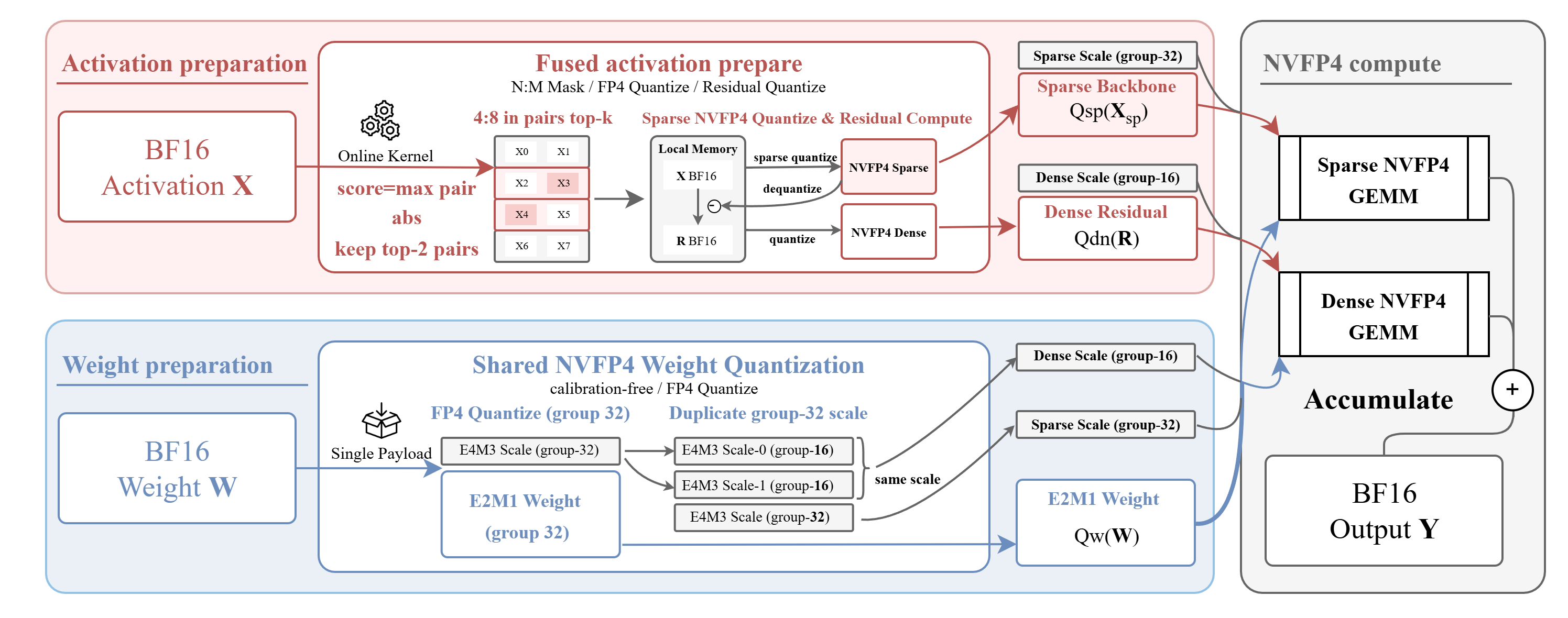
Fused sparse-residual preparation. The first efficiency challenge is that dynamic mask generation lies on the inference critical path. If implemented as a standalone step, its cost can easily offset the gain from sparse computation. SharQ addresses this by fusing mask selection with the preparation of both execution paths. In the current Blackwell NVFP4 implementation, the preparation kernel selects an outlier-dominated sparse backbone under a local 4:8 in-pairs constraint, quantizes and compresses it into the input format required by the sparse GEMM, and simultaneously constructs a dense residual relative to the quantized sparse backbone. The same preparation pipeline also produces the FP4 residual input for the dense compensation path. As a result, online mask generation is not exposed as a separate expensive operator, but absorbed into the activation preparation stage already required by the two-path computation. For layers with RMSNorm, SharQ further integrates normalization-aware preprocessing into this preparation pipeline, reducing additional activation transformation overhead.
Shared FP4 weights with path-specific scales. A naive two-path implementation would maintain one low-bit weight tensor for the sparse path and another for the dense path, increasing both storage cost and weight preparation overhead. SharQ instead keeps a single shared FP4 weight payload and lets both paths reuse the same low-bit weight body. The difficulty is that the two paths do not follow the same scale granularity: the dense NVFP4 path uses the standard dense scale organization, whereas the N:M sparse path follows the scale organization required by the sparse kernel. SharQ resolves this mismatch without duplicating the FP4 payload itself. It retains path-specific scale views on top of the shared weight representation, so that both the sparse path and the dense residual path can use scale layouts compatible with their own kernels while avoiding the storage and memory overhead of maintaining two separate quantized weight tensors.
Residual path compensation by accumulation. SharQ also avoids a naive two-branch output implementation. The sparse backbone is first processed by a sparse GEMM to produce the main output contribution. The dense residual path is then applied as a dense NVFP4 GEMM that accumulates directly into this output, rather than materializing a second full branch result and merging it afterward. This implementation matches the algorithmic role of the residual path: it is not an equally weighted parallel branch, but a compensation path for the information and quantization error left by the sparse path. More importantly, accumulation-based compensation removes an extra output writeback and readback, allowing the two-path decomposition to preserve a dataflow close to that of a single linear kernel. Combined with fused activation preparation and shared-weight design, this makes SharQ an efficiency-oriented inference primitive rather than a decomposition that exists only at the algorithmic level.
3.5 Theoretical analysis↩︎
We briefly explain SharQ from two perspectives: distribution and error. Since SharQ is primarily designed to improve activation representation under a fixed low-bit weight execution path, we focus on its activation-side compensation effect, namely how the online decomposition restructures activation approximation errors.
Outlier isolation improves activation quantization friendliness. In group-wise FP4 quantization, the local scale is typically determined by the largest magnitude within each group. A few outliers can therefore reduce the effective resolution available to ordinary activation values. By extracting these outlier-dominated components online into the sparse backbone, SharQ prevents the dense residual path from sharing the same dominant scale with them. The residual activation thus has a more concentrated local dynamic range and is better suited to dense low-bit FP4 representation. In this sense, SharQ does not merely sparsify activations; it reorganizes the activation distribution seen by the subsequent quantizer.
SharQ converts coupled activation errors into a single residual reconstruction problem. Let the actual activation represented by the sparse path be \[\widetilde{\mathbf{X}}_{\mathrm{sp}} = \mathcal{D}_{\mathrm{sp}} \left( \mathcal{Q}_{\mathrm{sp}}(\mathbf{X}_{\mathrm{sp}}) \right).\] SharQ defines the residual as \[\mathbf{R} = \mathbf{X} - \widetilde{\mathbf{X}}_{\mathrm{sp}}.\] Hence, \(\mathbf{R}\) contains both the information outside the sparse mask and the representation error introduced when the retained backbone is activation-quantized. If the dense path reconstructs the residual as \(\widetilde{\mathbf{R}}\), the final activation reconstruction error satisfies \[\mathbf{X} - (\widetilde{\mathbf{X}}_{\mathrm{sp}} + \widetilde{\mathbf{R}}) = \mathbf{R} - \widetilde{\mathbf{R}}.\] This shows that SharQ does not correct sparsification error and quantization error separately; it converts them into a single residual reconstruction problem. Furthermore, under a fixed weight operator \(\bar{\mathbf{W}}\), the output perturbation induced by activation approximation satisfies \[\| \mathbf{X}\bar{\mathbf{W}} - (\widetilde{\mathbf{X}}_{\mathrm{sp}} + \widetilde{\mathbf{R}})\bar{\mathbf{W}} \|_F \le \| \mathbf{R} - \widetilde{\mathbf{R}} \|_F \, \| \bar{\mathbf{W}} \|_2.\] Therefore, the key role of SharQ is not to make the sparse path reconstruct all activations accurately by itself, but to let the residual path jointly absorb sparse approximation loss and activation quantization loss.
4 Experiments↩︎
4.1 Experimental setup↩︎
We evaluate SharQ on three representative LLMs spanning different architectures and scales: Llama-3.1-8B [36] and Qwen2.5-7B [37] as standard dense decoder-only models, and Qwen3-30B-A3B [38] as a Mixture-of-Experts model with 30B total parameters and approximately 3B active parameters per token. This selection covers both dense and sparse-activated architectures.
The primary baseline is NVFP4 quantization applied to both activations and weights without any sparsity. FP16 serves as the full-precision reference. SharQ is applied on top of NVFP4 using the 4:8 in-pairs sparsity pattern supported by Blackwell Tensor Cores, without any training or calibration data.
We report zero-shot and few-shot accuracy on five standard benchmarks: ARC-Challenge [39], HellaSwag [40], Lambada [41], PIQA [42], and WinoGrande [43], along with their unweighted average. We additionally report perplexity on WikiText2 [44] (lower is better) and few-shot accuracy on MMLU [45] as complementary metrics that are particularly sensitive to quantization degradation. All evaluations are conducted using the Language Model Evaluation Harness [46].
4.2 Main results↩︎
Table ¿tbl:tab:main-results? summarizes the main results. Across all three models, SharQ consistently recovers a substantial portion of the accuracy lost by NVFP4 quantization. On Llama-3.1-8B, SharQ raises the average zero-shot accuracy from 70.32% (NVFP4) to 71.55%, closing roughly 56% of the 2.18 pp gap to FP16. WikiText2 perplexity improves from 6.94 to 6.73, and MMLU accuracy increases by 1.83 pp (61.93 \(\to\) 63.76). A similar pattern holds for Qwen2.5-7B, where SharQ recovers 63% of the average accuracy gap (69.43 \(\to\) 70.38 versus 70.94 for FP16) and reduces WikiText2 perplexity from 7.29 to 7.15.
3.5pt
@l|l|cccccc|c|c@ Model & Method & ARC-C & HellaSwag & Lambada & PIQA & WinoGrande & Avg. & WikiText2\(\downarrow\) & MMLU
& FP16 & 53.50 & 78.96 & 75.33 & 81.23 & 73.48 & 72.50 & 6.25 & 65.24
& NVFP4 & 49.91 & 77.41 & 74.02 & 79.60 & 70.64 & 70.32 & 6.94 & 61.93
& SharQ & 51.96 & 78.40 & 74.67 & 80.20 & 72.53 & 71.55 & 6.73 & 63.76
& FP16 & 51.01 & 78.94 & 71.92 & 79.92 & 72.93 & 70.94 & 6.85 & 74.16
& NVFP4 & 51.19 & 77.55 & 70.37 & 78.73 & 69.30 & 69.43 & 7.29 & 72.06
& SharQ & 52.73 & 78.08 & 70.00 & 79.43 & 71.67 & 70.38 & 7.15 & 72.83
& FP16 & 56.31 & 77.72 & 64.86 & 80.58 & 70.88 & 70.07 & 8.70 & 79.64
& NVFP4 & 54.52 & 76.76 & 62.91 & 78.35 & 69.46 & 68.40 & 9.12 & 77.72
& SharQ & 53.92 & 77.02 & 64.41 & 79.76 & 70.72 & 69.17 & 8.96 & 78.79
About the results on Qwen3-30B-A3B, SharQ improves the average accuracy from 68.40% to 69.17% and MMLU from 77.72% to 78.79%, demonstrating that the decomposition strategy remains effective when activations are routed through expert-specific linear layers. Notably, the largest per-benchmark gains appear on tasks most affected by quantization: Lambada improves by 1.50 pp and WinoGrande by 1.26 pp, both of which are sensitive to the representation quality of contextual activations.
All improvements are obtained without any training, calibration data, or model-specific tuning, confirming that SharQ operates as a plug-and-play inference primitive.
Multimodal evaluation. To assess whether SharQ generalizes beyond text-only language models, we further evaluate it on Qwen3-VL-8B [38], [47], a vision-language model, across five standard multimodal benchmarks: VQAv2 [48], GQA [49], ScienceQA [50], POPE [51], and TextVQA [52]. Table 1 reports the results.
| Method | VQAv2 | GQA | SQA | POPE | TextVQA | Avg. |
|---|---|---|---|---|---|---|
| FP16 | 81.84 | 61.54 | 92.76 | 89.14 | 81.58 | 81.37 |
| NVFP4 | 80.47 | 60.58 | 91.58 | 87.73 | 79.47 | 79.97 |
| SharQ | 81.10 | 61.04 | 91.96 | 88.20 | 80.57 | 80.57 |
SharQ consistently recovers accuracy across all five multimodal benchmarks. NVFP4 quantization degrades the average accuracy from 81.37% to 79.97% (a 1.40 pp drop); SharQ recovers this to 80.57%, closing approximately 43% of the gap to FP16. The improvement is broad-based: SharQ improves over NVFP4 on every benchmark, with gains ranging from 0.38 pp (SQA) to 1.10 pp (TextVQA). Notably, TextVQA exhibits both the largest NVFP4 degradation (\(-\)2.11 pp from FP16) and the highest SharQ recovery rate (52%), consistent with the observation that tasks requiring fine-grained visual-textual understanding are more sensitive to activation representation quality. POPE accuracy, which measures hallucination resistance, also improves by 0.47 pp (87.73 \(\to\) 88.20), indicating that SharQ’s decomposition preserves the cross-modal alignment needed for faithful visual grounding. These results demonstrate that SharQ’s online sparse–dense decomposition is effective not only for unimodal text generation but also for vision-language architectures where activations encode both visual and textual information.
4.3 Efficiency↩︎
We evaluate the end-to-end efficiency of SharQ on two representative workloads: autoregressive language model serving and diffusion-based video generation.
Language model serving. We integrate SharQ into vLLM [53] and benchmark on an NVIDIA RTX 5090 GPU with Llama-3.1-8B, comparing against FP16 (full-precision) and FP8 (weight-and-activation quantization) baselines under a fixed batch size of 4, sweeping input sequence lengths from 256 to 2048 with equal-length decode. Figure 3 summarizes the results.
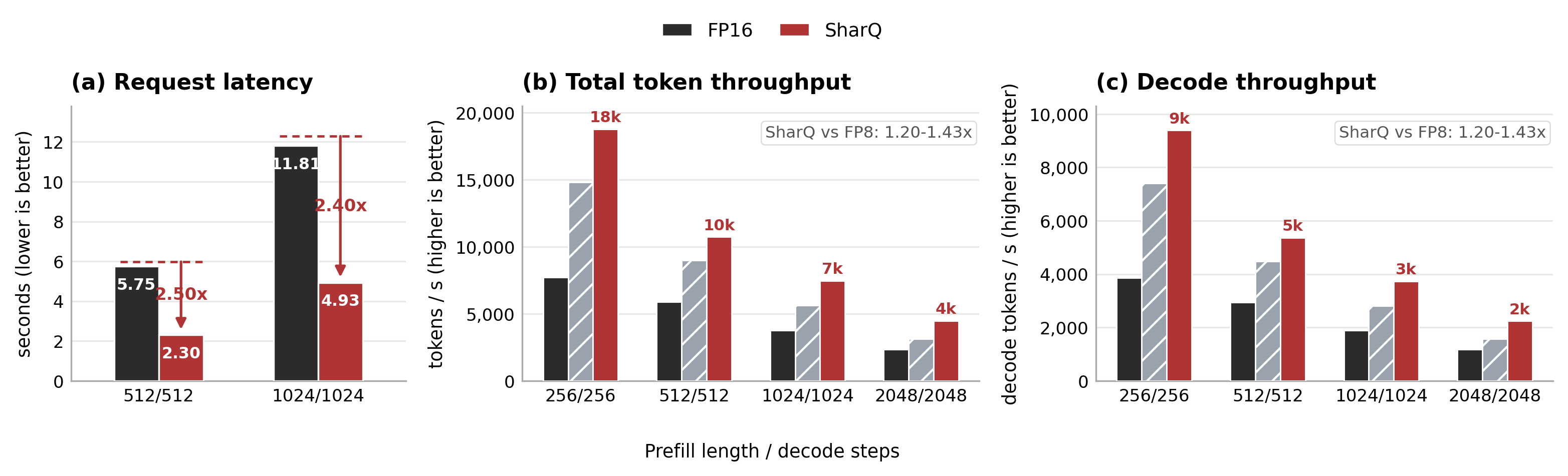
SharQ achieves substantial and consistent efficiency gains across all sequence lengths. Compared to FP16, SharQ reduces request latency by 55–60%: from 2.85 s to 1.17 s at seqlen = 256 (2.4\(\times\) speedup) and from 24.88 s to 11.11 s at seqlen = 2048 (2.2\(\times\) speedup). In terms of total token throughput, SharQ delivers 1.8–2.4\(\times\) higher tokens/s than FP16 across all configurations. Compared to FP8 quantization, SharQ still provides 1.2–1.4\(\times\) higher total token throughput across all sequence lengths. At seqlen = 2048, SharQ achieves 4 491 total tokens/s versus 3 146 for FP8 (1.43\(\times\)), demonstrating that the combination of sparse FP4 execution and dense FP4 residual compensation outperforms uniform FP8 even at longer contexts where memory bandwidth pressure is highest.
Video generation. To demonstrate the generality of SharQ beyond autoregressive LLMs, we evaluate it on Wan2.2-T2V-A14B [19], a state-of-the-art text-to-video diffusion model with 14B parameters. We measure end-to-end generation latency on 4\(\times\) RTX 5090 GPUs at 480P and 720P resolutions. We additionally evaluate SharQ combined with SageAttention [54] (SharQ+Sage), which applies efficient attention to further accelerate the diffusion denoising loop. Table 2 reports the results.
| Method | 480P | 720P |
|---|---|---|
| FP16 | 223.41 | 717.88 |
| SharQ | 182.21 (1.23\(\times\)) | 648.04 (1.11\(\times\)) |
| SharQ+Sage | 141.63 (1.58\(\times\)) | 457.88 (1.57\(\times\)) |
SharQ alone reduces 480P generation latency from 223.41 s to 182.21 s (1.23\(\times\) speedup, saving 41 s per video), and 720P latency from 717.88 s to 648.04 s (1.11\(\times\)). The more modest relative gain at 720P reflects the larger proportion of attention computation at higher resolution, which is not targeted by SharQ’s linear-layer optimization. When combined with SageAttention, the two techniques are complementary: SharQ+Sage achieves 141.63 s at 480P (1.58\(\times\) over FP16) and 457.88 s at 720P (1.57\(\times\)), reducing generation time by over 36% at both resolutions. These results demonstrate that SharQ generalizes beyond autoregressive decoding to iterative diffusion workloads, and composes naturally with orthogonal attention-level optimizations.
The efficiency advantages across both workloads stem from two complementary mechanisms. First, the sparse FP4 backbone exploits hardware-accelerated N:M semi-structured sparsity on Blackwell Tensor Cores, effectively halving the arithmetic cost of the dominant linear-layer computation. Second, the fused sparse-residual preparation kernel (Section 3.5) absorbs dynamic mask generation and residual construction into the activation preparation stage without introducing a separate preprocessing step. Combined with shared FP4 weights across both paths, SharQ maintains near-single-kernel data flow while exploiting two complementary execution paths.
4.4 Ablation study↩︎
We conduct two ablation studies to validate the design choices of SharQ.
Generalization across FP4 formats. Table 3 evaluates SharQ on three distinct FP4 numeric formats: NVFP4 [1] (with 4:8 in-pairs sparsity), HiF4 [4] (with 2:4 sparsity), and MXFP4 [3] (the OCP Microscaling standard). On Qwen3-30B-A3B, SharQ consistently improves all three formats across every benchmark. For NVFP4, WikiText2 perplexity drops from 9.12 to 8.96 and HellaSwag accuracy rises from 76.76% to 77.02%. For HiF4, the same pattern holds: perplexity improves from 9.08 to 8.92 and HellaSwag from 76.38% to 77.22%. The improvement is most pronounced on MXFP4, the weakest baseline due to its power-of-two scale constraint and larger group size: SharQ reduces WikiText2 perplexity from 9.70 to 9.19 (\(-\)0.51) and lifts HellaSwag by +1.36pp, Lambada by +2.84pp, Winogrande by +1.82pp, and BoolQ by +0.80pp. Across all three formats, BoolQ accuracy recovers toward the FP16 level, and the gains are consistent in both direction and magnitude. These results confirm that SharQ’s decomposition strategy is format-agnostic and benefits any block-scaled FP4 format paired with hardware-supported semi-structured sparsity.
| Method | HellaSwag | Lambada | WinoGrande | BoolQ | WikiText2\(\downarrow\) |
|---|---|---|---|---|---|
| FP16 | 77.72 | 64.86 | 70.88 | 88.62 | 8.70 |
| NVFP4+RTN | 76.76 | 62.91 | 69.46 | 87.77 | 9.12 |
| SharQ+NVFP4 | 77.02 | 64.41 | 70.72 | 88.41 | 8.96 |
| HiF4+RTN | 76.38 | 63.28 | 70.17 | 87.61 | 9.08 |
| SharQ+HiF4 | 77.22 | 64.08 | 70.24 | 88.07 | 8.92 |
| MXFP4+RTN | 74.77 | 59.71 | 67.48 | 86.91 | 9.70 |
| SharQ+MXFP4 | 76.13 | 62.55 | 69.30 | 87.71 | 9.19 |
Sparse–dense path combinations. Table 4 isolates the contribution of each path in SharQ by varying the combination of sparse and dense computation under NVFP4 on Llama-3.1-8B. Using only the sparse path without residual compensation (“Sparse”) is catastrophic: WikiText2 perplexity degrades to 82.95 and MMLU drops to 25.78%, confirming that discarding all non-outlier activation information destroys model quality. “Dense+Dense” applies two dense NVFP4 paths and achieves strong accuracy (WikiText2 6.63, MMLU 63.61), but forgoes the latency benefit of semi-structured sparse computation. “Sparse+Sparse” uses two sparse paths and yields results comparable to the NVFP4 baseline (WikiText2 6.95, MMLU 61.93), indicating that doubling the sparse computation without a dense compensation signal does not recover the sparsification loss. SharQ combines a sparse backbone with a dense residual, achieving WikiText2 6.73 and MMLU 63.76. This matches or exceeds the accuracy of the fully dense two-path variant while retaining the sparse execution path for the backbone, validating that the asymmetric sparse-plus-dense decomposition is the key to SharQ’s accuracy-efficiency trade-off.
| Combination | WikiText2\(\downarrow\) | MMLU | BoolQ | ARC-E |
|---|---|---|---|---|
| Sparse | 82.95 | 25.78 | 57.03 | 36.74 |
| Dense + Dense | 6.63 | 63.61 | 81.22 | 76.98 |
| Sparse + Sparse | 6.95 | 61.93 | 79.45 | 77.61 |
| SharQ | 6.73 | 63.76 | 80.58 | 77.74 |
Prefill latency breakdown and GEMM speedup. Figure 4 provides a fine-grained breakdown of the prefill latency on Llama-3.1-8B and compares per-kernel GEMM latency across different configurations.
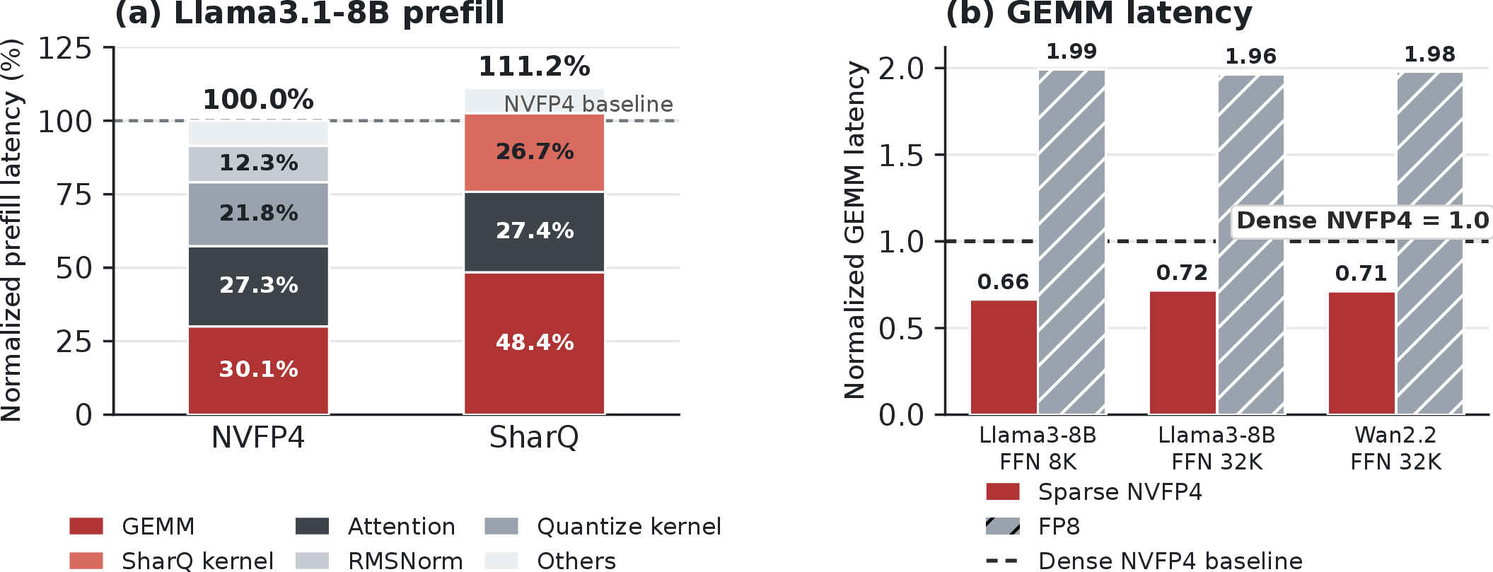
As shown in Figure 4 (a), the total prefill latency of SharQ is 111.2% relative to NVFP4, representing only an 11.2% overhead. This modest increase results from two opposing effects. On one hand, SharQ’s two-path execution (sparse backbone plus dense residual) increases the GEMM portion from 30.1% to 48.4% of the NVFP4 baseline time, as two matrix multiplications are issued per layer. On the other hand, the fused SharQ kernel absorbs both the standalone quantization kernel (12.3% in NVFP4) and the RMSNorm operator (21.8% in NVFP4) into a single kernel that jointly performs FP16-to-FP4 quantization, N:M sparse mask selection and compression, and layer normalization. This fusion reduces the combined preprocessing cost from 34.1% to 26.7%, saving 7.4 percentage points of prefill time. The net effect is that SharQ introduces only a small overhead during prefill while providing substantial accuracy recovery, and its end-to-end latency advantage manifests primarily in the decode phase where the sparse GEMM path dominates.
Figure 4 (b) isolates the GEMM kernel latency, normalized to dense NVFP4 as 1.0. Sparse NVFP4 achieves 0.66\(\times\), 0.72\(\times\), and 0.71\(\times\) of the dense NVFP4 GEMM latency on Llama-3.1-8B FFN 8K, Llama-3.1-8B FFN 32K, and Wan2.2 FFN 32K respectively, corresponding to a 28–34% GEMM speedup from the 4:8 semi-structured sparsity. In contrast, FP8 GEMMs require approximately 2\(\times\) the latency of dense NVFP4 (1.99\(\times\), 1.96\(\times\), 1.98\(\times\)), confirming that FP4 formats offer a fundamental compute density advantage over FP8. These kernel-level measurements validate SharQ’s design: the sparse FP4 backbone exploits hardware-accelerated N:M sparsity for significant arithmetic savings, while the fused preparation kernel ensures that the overhead of online decomposition does not erode the throughput gains.
5 Conclusion↩︎
We presented SharQ, a training-free inference method that combines activation sparsity with FP4 quantization through an online sparse/dense decomposition. An input-adaptive N:M mask extracts an outlier-dominated sparse backbone for hardware-accelerated sparse FP4 computation, and a dense FP4 residual, defined relative to the quantized sparse backbone, jointly compensates for mask-induced activation loss and sparse-path quantization error. Three implementation choices make this decomposition practical: a fused preparation kernel that absorbs mask generation, residual construction, and layer normalization into a single operator; shared FP4 weights with path-specific scale views; and accumulation-based residual compensation that preserves near-single-kernel data flow. Experiments on dense decoder-only models (Llama-3.1-8B, Qwen2.5-7B), a mixture-of-experts model (Qwen3-30B-A3B), a vision-language model (Qwen3-VL-8B), and a video generation model (Wan2.2-T2V-A14B) show that SharQ consistently recovers a substantial fraction of FP4 quantization accuracy loss while delivering 2.2–2.4\(\times\) latency reduction over FP16 and 1.2–1.4\(\times\) throughput improvement over FP8 in language model serving. The same mechanism generalizes across NVFP4, HiF4, and MXFP4 without modification, confirming its format-agnostic nature. SharQ requires no calibration data, retraining, or model-specific tuning, operating as a plug-and-play inference primitive wherever block-scaled FP4 and N:M semi-structured sparsity are available.
6 Supplementary Materials↩︎
6.1 NVFP4 Data Format↩︎
This section describes the NVFP4 block floating-point format used as the primary quantization target in our experiments. NVFP4 is a proprietary format introduced with the NVIDIA Blackwell architecture that improves upon the OCP MXFP4 standard by addressing two key limitations of prior block-scaled FP4 designs.
6.1.1 Design rationale↩︎
MXFP4 (OCP Microscaling FP4) uses E2M1 elements with a shared power-of-two 8-bit exponent (E8M0) and a group size of 32, yielding an average storage cost of 4.25 bits per value. However, the power-of-two constraint on the block scale cannot guarantee normalization of each group’s peak magnitude to the representable upper bound of E2M1, wasting intra-group dynamic range. NVFP4 introduces two changes to address this:
Floating-point block scale. NVFP4 replaces the power-of-two E8M0 scale with a fine-grained FP8-E4M3 floating-point scale. This allows the scale to normalize group peaks more precisely to the upper bound of E2M1, fully utilizing the intra-group expressive space.
Smaller group size. NVFP4 adopts a 16-element group size (reduced from 32 in MXFP4), raising the average storage cost from 4.25 to 4.5 bits per value but effectively reducing outlier-driven quantization error by providing finer-grained scaling granularity.
6.1.2 Format structure↩︎
An NVFP4 block consists of 16 four-bit E2M1 elements sharing a single FP8-E4M3 block scale, for a total storage of \(16 \times 4 + 8 = 72\) bits, or 4.5 bits per value. The E2M1 element format allocates 2 bits to the exponent and 1 bit to the mantissa (with an implicit leading 1 for normal values), plus 1 sign bit. The representable nonzero magnitudes in E2M1 are \(\{0.5, 1.0, 1.5, 2.0, 3.0, 4.0, 6.0\}\), with the maximum value being 6 and special encodings reserved for \(\pm 0\) and NaN.
The FP8-E4M3 block scale uses 4 exponent bits (bias 7) and 3 mantissa bits, providing a scale dynamic range of \([-10, 11]\) in binades (22 binades total). Combined with the E2M1 element range, the local intra-group dynamic range is \(\log_2(6/0.5) = 3.58\) binades.
6.1.3 Per-tensor scaling↩︎
Because the E4M3 block scale provides only 22 binades of global dynamic range, NVFP4 requires an additional software-based per-tensor scaling (PTS) step before format conversion. PTS normalizes each tensor’s peak magnitude to a target value (typically 2688 for activations) so that the E4M3 scale range is sufficient to cover the tensor’s value distribution. This additional preprocessing step incurs some overhead during inference but is necessary to prevent overflow and underflow in the block scale.
6.1.4 Sparsity support↩︎
On the Blackwell architecture, NVFP4 natively supports 4:8 semi-structured sparsity in pairs. Within each group of 8 consecutive elements (organized as 4 pairs), the hardware retains 4 elements (2 pairs) and prunes the remaining 4. This “in-pairs” constraint means that sparsity selection operates on pairs of adjacent elements rather than individual values, which simplifies hardware metadata encoding while still enabling effective activation sparsity. SharQ exploits this 4:8 in-pairs pattern as the sparse backbone constraint in its NVFP4 instantiation.
6.1.5 Comparison with other FP4 formats↩︎
Table 5 summarizes the key differences between NVFP4 and other block-scaled FP4 formats.
| Feature | MX4 | MXFP4 | NVFP4 |
|---|---|---|---|
| 4-bit Element | S1P1 | E2M1 | E2M1 |
| Block Scale Format | E8M0 | E8M0 | E4M3 |
| Group Size | 16 | 32 | 16 |
| Storage Cost | 4.0 bits | 4.25 bits | 4.5 bits |
| Scale Type | Power-of-2 | Power-of-2 | Floating-point |
| Significand Precision | 2 bits | 2 bits | 2 bits |
| Local Dynamic Range | 2.81 binades | 3.58 binades | 3.58 binades |
| Global Dynamic Range | N/A | N/A | 22 binades |
| Requires PTS | No | No | Yes |
NVFP4 achieves better quantization accuracy than MXFP4 by combining the floating-point scale (which fully utilizes E2M1’s representable range) with a smaller group size (which reduces the impact of outliers within each block). However, the limited global dynamic range of E4M3 necessitates per-tensor scaling, and the smaller group size increases metadata overhead. These trade-offs position NVFP4 as a format optimized for inference accuracy on current hardware, while formats like HiF4 (Appendix 6.2) explore alternative designs with wider dynamic range and lower hardware cost.
6.2 HiFloat4 (HiF4) Data Format↩︎
This section provides a detailed description of the HiFloat4 (HiF4) block floating-point format, which is one of the FP4 numeric formats evaluated in our ablation study (Table 3). HiF4 was proposed as a high-fidelity 4-bit BFP format for deep learning inference and training. We summarize its structure, encoding, and key differences from NVFP4 to make the paper self-contained.
6.2.1 Format overview↩︎
A basic HiF4 unit packs 64 four-bit in-group elements together with 32 bits of shared scaling metadata, resulting in an average storage cost of 4.5 bits per value (identical to NVFP4). The distinguishing feature of HiF4 is a three-level scaling hierarchy that captures both inter-group and intra-group dynamic range variation, improving representational utilization compared with single- or two-level scaling designs.
6.2.2 Three-level scaling metadata↩︎
The 32-bit scaling metadata is organized into three hierarchical levels:
Level-1: Global base scale (E6M2). The first level is a specially designed unsigned 8-bit floating-point format called E6M2. It assigns 6 bits to the exponent field with a bias of 48 and 2 bits to the mantissa field with one hidden integer bit set to 1. E6M2 encodes NaN (Not a Number) but does not support infinity or zero; only normal mode is used. If we denote the unbiased exponent as \(E\) and the mantissa as \(M\), an E6M2 value is interpreted as \[X = 2^{E} \times 1.M . \label{eq:e6m2}\tag{10}\] This scale provides a wide dynamic range across groups (unbiased exponent range \([-48, 15]\)) and normalizes each group’s peak magnitude to the representable upper bound of the remaining hierarchical structure, ensuring full utilization of the intra-group dynamic range.
Level-2: 8-way one-bit micro-exponents (E1_8). The second level consists of 8 one-bit micro-exponents, each shared by 8 consecutive in-group elements. Each E1 bit encodes either 1 or 0, representing a very fine-grained power-of-two scaling factor (\(2^{E1}\) collapses to either \(2\) or \(1\)). Each level-2 E1 further connects to two adjacent level-3 micro-exponents.
Level-3: 16-way one-bit micro-exponents (E1_16). The third level consists of 16 one-bit micro-exponents, each shared by 4 contiguous four-bit elements within its local group. Together with the level-2 micro-exponents, these refine the intra-group dynamic range by capturing local exponent differences, effectively mitigating the impact of outliers and suppressing quantization error.
All three levels of scaling metadata occupy 32 bits in total (\(8 + 8 + 16\)), distributed over 64 in-group elements, leading to an extra overhead of 0.5 bits per value.
6.2.3 Element encoding: S1P2↩︎
HiF4 encodes the 64 four-bit in-group elements using the sign-magnitude S1P2 representation. In the SXPY notation, S denotes the sign bit and P indicates the binary point; the value X preceding P designates the integer part, and the value Y following P designates the fractional part. Conceptually, S1P2 is equivalent to the E1M2 format in floating-point representation. The encoding details are summarized in Table 6.
| Property | Unsigned FP8-E6M2 | Sign-Magnitude S1P2 |
|---|---|---|
| Exponent Bias | 48 | N/A |
| Unbiased Exp | \([-48,\;15]\) | N/A |
| Infinity | N/A | N/A |
| Zero | N/A | \(\text{S}0.00_2 = \pm 0.00\) |
| NaN | \(111111\_11_2\) | N/A |
| Max Value | \(111111\_10_2 = 2^{15} \times 1.50\) | \(\text{S}1.11_2 = \pm 1.75\) |
| Min Value | \(000000\_00_2 = 2^{-48} \times 1.00\) | \(\text{S}0.01_2 = \pm 0.25\) |
6.2.4 Value representation↩︎
Based on the three-level hierarchy, each of the 64 real numbers \(\{V_i\}_{i=1}^{64}\) in a HiF4 group can be expressed as follows. If \(\text{E6M2} = \text{NaN}\), then \(V_i = \text{NaN}\) for all \(i \in [1, 64]\). Otherwise, \[V_i = \text{E6M2} \times 2^{\left(\{\text{E1\_8}\}_{\lfloor i/8 \rfloor} + \{\text{E1\_16}\}_{\lfloor i/4 \rfloor}\right)} \times \{\text{S1P2}\}_i , \label{eq:hif4-value}\tag{11}\] where \(\{\text{E1\_8}\}_j\) (\(j \in [1,8]\)) and \(\{\text{E1\_16}\}_k\) (\(k \in [1,16]\)) denote the level-2 and level-3 micro-exponents, respectively. The available intra-group dynamic range of HiF4 is \(\log_2(7/0.25) = 4.81\) binades, since the maximum positive value within a group is \(2^{(1+1)} \times 1.75 = 7\) and the minimum positive value is \(2^{(0+0)} \times 0.25 = 0.25\).
6.2.5 Comparison with NVFP4↩︎
Table 7 compares the key features of HiF4 and NVFP4. Despite identical average storage costs, HiF4 offers a substantially wider global dynamic range (69 vs. binades), higher significand precision (3 bits vs. bits), and a larger local dynamic range (4.81 vs. binades). These properties make HiF4 more robust to outlier-driven quantization error and reduce the need for software-based per-tensor scaling (PTS) that NVFP4 typically requires.
| Feature | HiF4 | NVFP4 |
|---|---|---|
| Storage Overhead | 4.5 bits/value | 4.5 bits/value |
| Group Size | 64 | 16 |
| Special Values | NaN and \(\pm 0\) | NaN and \(\pm 0\) |
| 4-bit Element | S1P2 (E1M2) | E2M1 |
| Significand Precision | 3 bits | 2 bits |
| Global Base Scale | E6M2 | E4M3 |
| Max Positive Value | \(2^{18} \times 1.3125\) | \(2^{11} \times 1.3125\) |
| Min Positive Value | \(2^{-50}\) | \(2^{-10}\) |
| Global Dynamic Range | \([-50,\;18]\): 69 binades | \([-10,\;11]\): 22 binades |
| Local Dynamic Range | 4.81 binades | 3.58 binades |
6.2.6 Conversion from BF16 to HiF4↩︎
Algorithm 5 outlines the conversion procedure from a 64-length BF16 vector to a HiF4 unit. The algorithm proceeds in three stages: (1) a three-level tree reduction to find local and global peak magnitudes; (2) derivation of the three-level hierarchical scaling metadata (E6M2, E1_8, E1_16); and (3) scaling and quantization of the 64 in-group elements into S1P2 format. All rounding operations use round-half-to-even or round-half-away-from-zero. The E6M2 reciprocal computation can be efficiently implemented using only a 4-entry lookup table indexed by the 2-bit mantissa, combined with simple exponent subtraction.
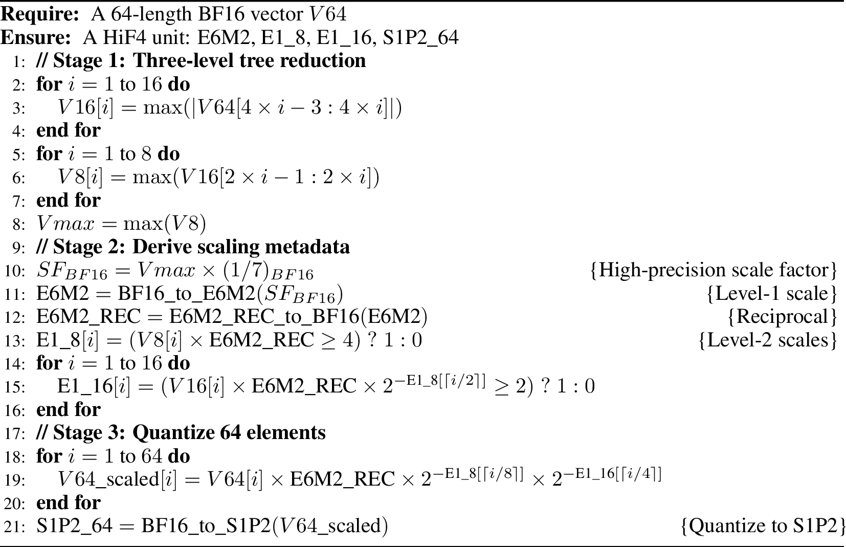
For the HiF4 dot product, level-2 and level-3 micro-exponents can be implemented as simple left-shift operations in hardware. When integrated into existing 64-length dot-product units originally optimized for 16-bit and 8-bit formats, HiF4 occupies only approximately one-third the incremental area of NVFP4 and reduces power consumption by about 10%, enabling a more area- and power-efficient implementation for matrix multiplication.