1 Introduction↩︎

Computing shortest paths is among the most fundamental problems in computer science. Many of its variants have been studied in the literature, and the All-Pairs Shortest Paths (APSP) problem is one of the most fundamental variants and has been extensively studied.

In APSP, one needs to compute the distance between every pair of nodes in a given \(n\)-vertex graph.² One could run Dijkstra’s algorithm \(n\) times to obtain an \(O(n^{3})\) running time. An alternative classical algorithm, the Floyd–Warshall algorithm, also achieves an \(O(n^3)\) running time. A long series of works (e.g. [1]–[11]) improved poly-logarithmic factors over the classic \(O(n^3)\) running time, culminating in the current fastest algorithm by Williams [12] with \(n^3 / 2^{\Theta(\sqrt{\log n})}\) running time for general weighted graphs, a super poly-logarithmic improvement over the classic \(O(n^3)\) running time. Due to the lack of polynomial improvements, the APSP hypothesis, stating that there is no \(O(n^{3-\varepsilon})\) time algorithm for any \(\varepsilon>0\) that computes APSP for \(n\)-node graphs, is among the most popular hypotheses in Fine-Grained Complexity.

Faster algorithms are known in unweighted graphs. If the graph is undirected, Seidel [13] gave an algorithm computing APSP in \(\widehat{O}(n^{\omega})\) time.³ More generally, on undirected graphs with positive integer weights bounded by \(B\), APSP can be computed in \(\widehat{O}(Bn^{\omega})\) time [15], [16]. For directed unweighted graphs, the current fastest algorithm was designed by Zwick [17], which runs in \(O(n^{2.528})\) time.

A simpler version of distance problems is reachability problems, where one needs to decide whether a vertex can reach another vertex. All-Pairs Reachability, also popularly known as transitive closure, is another fundamental problem in graph algorithms. It is known to be equivalent to the Boolean Matrix Multiplication problem, and can be solved in \(\widehat{O}(n^\omega)\) time [18], [19].

Computing all the pairwise distances (resp. reachability) gives full distance (resp. reachability) information of the graph, but it also comes with a cost: it is computationally expensive. In contrast, computing the distance between a fixed pair of vertices only takes near-linear time in all the variants mentioned above, though it gives much less information than APSP. A natural question is to study the intermediate cases:

Graphs arising in theory and practice applications often contain a small set of hot spots, where distances between these hot spots and other vertices are more likely to be queried. For instance, in the network connecting all locations in a city, distances from places like grocery stores, shopping malls and parks are more likely to be queried than distances between two residential buildings. In theory, many applications using distance computations only need distances from a fixed small set of vertices to other vertices (e.g. approximate APSP [20]–[24], approximate diameter [25]–[27] and shortcut sets and hopsets [28]).

Motivated by these applications, we study the multiple source version of distance and reachability problems. More formally, we study:

1.1 Shortest Paths in Undirected Unweighted Graphs↩︎

Our first result is for Multiple-Source Shortest Paths in undirected unweighted graphs. There are two straightforward algorithms to solve MSSP: we can either solve SSSP for every \(s \in S_{\mathrm{in}}\), or solve APSP. For undirected graphs, there were no other known algorithms besides these two approaches, to the best of our knowledge. This leads to the following question that motivated our work, instantiating a specific instance of 1.

We answer this question in the affirmative, giving the first algorithm that beats this running time. In fact, our algorithm is essentially optimal, by tying the running time of our algorithm to Boolean matrix multiplication.

Here, \(\mathrm{BMM}(a, b, c)\) denotes Boolean matrix product instances between \(a \times b\) matrices and \(b \times c\) matrices, and \(\mathsf{T}_{\mathrm{BMM}}(a, b, c)\) denotes the running time of such instances. In particular, \(\mathsf{T}_{\mathrm{BMM}}(a, b, c)\) can be upper bounded by the running time for computing products of general \(a \times b\) and \(b \times c\) matrices, utilizing fast matrix multiplication algorithms (see 1 for an illustration of the quantitative improvements we achieve). The reduction from Boolean matrix multiplication to MSSP in the above theorem can be achieved with standard approaches.⁵ We also extend our algorithm to handle graphs with small integer weights.

Here, \(\mathrm{MPP}(|S_{\mathrm{in}}|, n, n \mid B)\) denotes Min-Plus product between an \(|S_{\mathrm{in}}| \times n\) matrix and an \(n \times n\) matrix, whose entries are from \([B] \cup \{\infty\}\), and \(\mathsf{T}_{\mathrm{MPP}}(|S_{\mathrm{in}}|, n, n \mid B)\) denotes the running time of such instances. It is known that \(\mathsf{T}_{\mathrm{MPP}}(a, b, c \mid B) = \widetilde{O}\left(B \mathsf{T}_{\mathrm{MUL}}(a, b, c)\right)\) [16].

Our algorithms give a smooth interpolation between the SSSP algorithm and the APSP algorithms [13] and [15]. When \(s = n\), our algorithm serves as an alternative algorithm for APSP in undirected graphs with unit or small integer weights (See [29] for another alternative algorithm).

The key technical ingredient of our algorithms is a novel low diameter decomposition, which may be of independent interest. We define the notion of a low diameter small neighborhood decomposition. We say \(V_1 \sqcup \dots \sqcup V_{k}\) is a \((d, \phi)\)-low diameter small neighborhood decomposition if (1) \(\mathrm{diam}(G[V_i]) \leqslant d\) for all \(i\), and (2) \(\sum_{i} |N(V_i)| \leqslant\phi n\). While the first condition is reminiscent of standard low diameter decompositions, the second condition is different: instead of requiring that the number of edges between clusters is small (see e.g. [30]), our decomposition requires that the neighborhoods of the clusters are small. In particular, while there may be many edges incident to any given cluster, we ensure that they do not expand and hit too many distinct vertices. Note that our bound on the neighborhood size is global rather than local, there may be clusters where \(|N(V_i)| > \phi |V_i|\), but the sum of the neighborhoods is at most \(\phi n\). We show how to obtain an \((n^{o(1)}, n^{o(1)})\)-low diameter small neighborhood decomposition in \(n^{2 + o(1)}\) time.

We also give some natural applications of our MSSP algorithm. We obtain improvements over the state-of-the-art algorithms with simple reductions, establishing the practical impact of the MSSP problem (see 5.3 for formal statements).

1.1.0.1 Hop-sets.

A (weighted) set of edges \(F\) is a \(\beta\)-hop-set for graph \(G = (V, E)\) if every pair of vertices \((u, v)\) in \(H = (V, E \cup F)\) has the same distance as in \(G\) and there exists a shortest path of at most \(\beta\) hops. Research in hop-sets (and the related concept of shortcut sets) aims to minimize both the size of the hop-set (ideally linear) and the hop diameter \(\beta\). A folklore sampling algorithm produces \(\beta\)-hop-sets of size \(n^2/\beta^{2}\): sample a set \(S\) of \(n/\beta\) vertices, and add all edges between \((u, v) \in S \times S\) with weight \(\mathrm{dist}(u, v)\). In particular, we may obtain an \(\widetilde{O}\left(n^{1/2}\right)\)-hop-set of size \(\widetilde{O}\left(n\right)\). Bodwin and Hoppenworth showed that the folklore sampling is optimal up to polylogarithmic factors: any exact hop-set of size \(\widetilde{O}\left(n\right)\) must have \(\beta = \widetilde{\Omega}\left(n^{1/2}\right)\) [31].

However, the sampling algorithm does not compute a hop-set efficiently, since previous algorithms for computing all distances between \(S \times S\) for \(S\) of size \(\sqrt{n}\) require time \(\widehat{O}(\min(n^{2.5}, n^{\omega})) = O(n^{2.372})\). Our improved MSSP algorithm allows us to compute all \(S \times S\) distances in time \(n^{\omega(0.5, 1, 1)} = O(n^{2.043})\) [14].⁷

1.1.0.2 Distance Emulators.

Emulators are sparse graphs that faithfully preserve the distances of a graph. Formally, given a graph \(G=(V,E)\), a (possibly weighted) set of edges \(F\) is a \(+k\)-emulator if \(\mathrm{dist}_{G}(u, v) \leqslant\mathrm{dist}_{(V, F)}(u, v) \leqslant\mathrm{dist}_{G}(u, v) + k\) for all pairs of vertices \(u, v\). Emulators (and related constructions such as graph spanners) have been the subject of intense study since their introduction [32], and have been useful objects with many applications, including compact routing schemes [33]–[37], distance oracles [38], [39], and broadcasting [40].

Several constructions of additive emulators are known: \(+2\)-emulators of size \(\widetilde{O}\left(n^{3/2}\right)\) [41], \(+4\)-emulators of size \(\widetilde{O}\left(n^{4/3}\right)\) [42], and \(+6\)-emulators of size \(\widetilde{O}\left(n^{4/3}\right)\) [43]. We remark that both the \(+2\) and \(+6\) constructions are spanners (\(F\) is a subset of \(E\)). However, the sparsest \(+4\)-spanner known has size \(\widetilde{O}\left(n^{7/5}\right)\) [44]. Furthermore, it is known that no emulator (or any data structure) of size \(n^{4/3 - \Omega(1)}\) can achieve error \(k = n^{o(1)}\) [45]. Thus, significant effort has been devoted to characterizing the additive error of emulators of linear size [46]–[52].

Both the \(+2\) and \(+6\)-emulators can be constructed in near-linear time \(\widetilde{O}\left(n^2\right)\) [42], [53]. However, the best known algorithm for constructing the \(+4\)-emulator requires time \(\widetilde{O}\left(n^{7/3}\right)\) [42]. With our MSSP algorithm, we obtain a construction in time \(\widehat{O}(n^{\omega(2/3, 1, 1)}) = O(n^{2.1321})\) [14].

1.2 Reachability in Directed Graphs↩︎

In the Multiple-Source Reachability problem, the goal is to determine whether \(s\) can reach \(v\) for every pair \((s, v) \in S_{\mathrm{in}} \times V\). As all-pairs reachability can be solved in \(\widehat{O}(n^\omega)\) time [18], [19], and single-source reachability can be solved in \(O(m)\) time, Multiple-Source Reachability can be solved in \(\widehat{O}(\min(|S_{\mathrm{in}}| m, n^\omega))\) time, similar to MSSP on undirected unweighted graphs. Standard reduction from \(\mathrm{BMM}(S_{\mathrm{in}}, n, n)\) also works for Multiple-Source Reachability, establishing an \(\Omega(\mathsf{T}_{\mathrm{BMM}}(S_{\mathrm{in}}, n, n))\) lower bound.

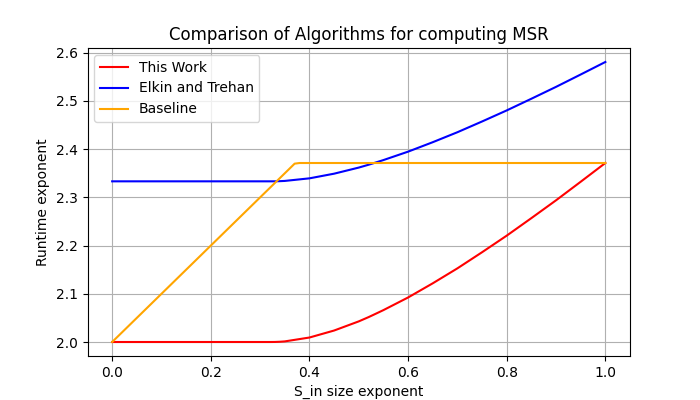
Recently, Elkin and Trehan [54], [55] gave an alternative algorithm for Multiple-Source Reachability. Their algorithm runs in \(\widehat{O}\left(n \mathsf{T}_{\mathrm{MUL}}(S_{\mathrm{in}}, n, n)^{2/3}\right)\), which beats \(\widehat{O}(\min(S_{\mathrm{in}} m, n^\omega))\) for certain values of \(|S_{\mathrm{in}}|\), but unfortunately never meets the \(\Omega(\mathsf{T}_{\mathrm{BMM}}(S_{\mathrm{in}}, n, n))\) lower bound (see 1).

In our second main result, we design an algorithm for Multiple-Source Reachability that matches the \(\Omega(\mathsf{T}_{\mathrm{BMM}}(S_{\mathrm{in}}, n, n))\) lower bound.

The following figure illustrates a comparison of our algorithm with the baseline algorithm and the algorithm of Elkin and Trehan [54], [55].

1.3 Shortest Paths in Directed Acyclic Unweighted Graphs↩︎

Finally, we study MSSP on directed unweighted graphs, whose running time landscapes seem to be more complicated. Consider APSP as an example. APSP for undirected unweighted graphs runs in \(\widehat{O}(n^\omega)\) time [13], while APSP for directed unweighted graphs runs in \(\widehat{O}(n^{2+\mu})\) time [17], where \(\mu \le 0.528\) [14] is the solution to \(\omega(1, \mu, 1) = 2 + \mu\). As we can see, even representing the running time requires more effort in the directed case.

One can rephrase the running time of Zwick’s algorithm as \[\widetilde{O}\left(\max_{1 \le t \le n} \mathsf{T}_{\mathrm{MPP}}(n, t, n \mid n / t)\right),\] as observed in [29]. In fact, [29] showed that the running time for APSP in directed unweighted graphs is exactly \[\widetilde{\Theta}\left(\max_{1 \le t \le n} \mathsf{T}_{\mathrm{MPP}}(n, n/t, n \mid t)\right).\] Grandoni and Vassilevska Williams [56] gave an algorithm that can solve MSSP on directed unweighted graphs⁸, and the running time of their algorithm can be phrased as (let \(s = |S_{\mathrm{in}}|\)) \[\label{eq:GV-time} \widetilde{O}\left(\max_{1 \le t \le n} \mathsf{T}_{\mathrm{MPP}}(s + t, t, n \mid n / t)\right),\tag{1}\] Based on the approach in [29], we can show the following lower bound for MSSP on directed unweighted graphs: \[\label{eq:directed-lower-bound} \Omega\left(\max_{1 \le t \le n} \mathsf{T}_{\mathrm{MPP}}(s, t, n \mid n / \min(s, t), n / t)\right),\tag{2}\] where \(\mathsf{T}_{\mathrm{MPP}}(a, b, c \mid B_1, B_2)\) denotes the running time for Min-Plus product instances between an \(a \times b\) matrix with entries from \([B_1] \cup \{\infty\}\) and a \(b \times c\) matrix with entries from \([B_2] \cup \{\infty\}\).

Grandoni and Vassilevska Williams’s algorithm [56] is actually optimal for sufficiently large \(s\). To see this, let \(s\) be large enough so that the maximizer \(t^*\) for 1 is less than or equal to \(s\). In this case, their running time simplifies to \(\widetilde{O}\left(\mathsf{T}_{\mathrm{MPP}}\left(s, t^*, n \mid n / t^*\right)\right)\), which matches \(\mathsf{T}_{\mathrm{MPP}}(s, t, n \mid n / \min(s, t), n / t)\) by setting \(t = t^*\). On the other hand, their running time is not optimal for small values of \(s\). By setting \(t = n\) in 1 , their running time is not better than \(\widetilde{O}\left(\mathsf{T}_{\mathrm{MPP}}\left(n, n, n \mid 1\right)\right) = \widetilde{\Theta}\left(\mathsf{T}_{\mathrm{BMM}}\left(n, n, n\right)\right)\). Hence, using fast matrix multiplication for Boolean matrix product (this is the currently best known algorithm for Boolean matrix product), their running time always has an \(n^\omega\) term, even for small values of \(s\).

We improve [56]’s algorithm for small values of \(s\), in the important special case of directed acyclic graphs:

Surprisingly, even though the running time expression for [thm:dag-mssp] is quite different from 2 , the numerical values of the exponents in \(n\) appear to match for small values of \(s\), utilizing the currently best known algorithm for Min-Plus product between two matrices that can have potentially different entry bounds. In fact, if we take the minimum of [56]’s algorithm and [thm:dag-mssp], the upper and lower bounds appear to be numerically matching for all values of \(s\)! Of course, this does not establish a formal lower bound, as there might be better algorithms for such Min-Plus product instances. See 7 for details.

1.3.0.1 Shortcut Sets

A set of edges \(F\) is a \(D\)-shortcut-set for graph \(G = (V, E)\) if \(H = (V, E \cup F)\) has the same transitive closure as \(G\) and \(\mathrm{diam}(G \cup F) \leqslant D\). For a directed graph, \(\mathrm{diam}(G) = \max_{(u, v) \in \mathrm{TC}(G)} \mathrm{dist}(u, v)\) is the maximum distance between any two vertices for \((u, v) \in \mathrm{TC}(G)\), where \(\mathrm{TC}(G)\) is the transitive closure of \(G\). Shortcut sets have applications in reachability and shortest paths computation in many settings [57]–[64]. Similar to exact hop-sets, a folklore sampling algorithm yields a shortcut set of diameter \(O(\sqrt{n})\) and size \(\widetilde{O}\left(n\right)\). A breakthrough result of Kogan and Parter [65] showed that in fact there exist shortcut sets of size \(\widetilde{O}\left(n\right)\) and diameter \(O(n^{1/3})\), while no linear size shortcut set can achieve diameter \(o(n^{1/4})\) [31], [66]. As with hop-sets, known algorithms for computing shortcut sets are not optimal, with the current best algorithm computing diameter \(D\)-shortcut-sets of size \(\widetilde{O}\left(n^2/D^3 + n\right)\) in time \(\widetilde{O}\left(mn/D^2\right) = \widetilde{O}\left(n^3 / D^2\right)\) whenever \(D = O(\sqrt{n})\) [67] ([68]’s running time is the same for dense graphs). As an application of [thm:dag-mssp], we compute shortcut-sets in dense graphs of diameter \(D\) and size \(\widetilde{O}\left(n^2/D^3 + n\right)\) in time \(\widetilde{O}\left(\mathsf{T}_{\mathrm{MPP}}(n/D^2, n, n \mid D, 1)\right)\) (see 12). Our algorithm is faster than [67] for all values of \(D = O(\sqrt{n})\), as illustrated in 2. For the important case \(D = n^{1/3}\), our running time is \(O(n^{2.064})\).

1.4 Related Works↩︎

1 is a long-term research paradigm that has been approached from many angles:

1. Single-Source Shortest Paths (SSSP): The most classical and successful example [69], [70], SSSP computes a set of \(n\) distances from \(s\).

2. Extremal distances: The diameter, radius, and eccentricities are well-studied problems in distance computation, resulting in both approximation algorithms [25]–[27], [71] and hardness results [25], [72], [73].

3. \(n\)-Pairs Shortest Paths (NPSP): Given \(n\) pre-specified pairs of vertices \((s_i, t_i)\), compute \(\mathrm{dist}(s_i, t_i)\) for all \(i\). In contrast to SSSP, the NPSP problem computes \(n\) arbitrary pre-specified distances. The study of NPSP was initiated by [41], with several recent works reigniting interest in the question [74], [75].

4. Distance Oracles: Preprocess \(G\) so that given any query \((u, v)\), return \(\mathrm{dist}(u, v)\) efficiently. Distance oracles capture the setting where we do not know what distances are interesting in advance. A long line of work has established a variety of approximation algorithms [38], [76]–[81] and hardness results [82]–[84].

1.5 Open Questions↩︎

We conclude the introduction with some open questions.

1. We establish an equivalence between BMM and MSSP on unweighted, undirected graphs. Can a similar equivalence (with some other matrix product) be established for MSSP on directed graphs? Concretely, can [thm:dag-mssp] be generalized to compute shortest paths on directed graphs (not necessarily DAGs)?

2. In our work, we have shown that a \((d, \phi)\)-low diameter small neighborhood decomposition can be computed efficiently, where \(d, \phi = n^{o(1)}\). In principle, it may be possible to obtain a decomposition where \(|N(V_i)| = O(|V_i|)\) and \(\mathrm{diam}(V_i) = O(\log n)\) for all \(V_i\). Can we obtain such a decomposition, and do so efficiently? Even the weaker setting where \(d, \phi = \mathrm{polylog}(n)\) would be interesting.

3. Our decomposition algorithm runs in \(n^{2 + o(1)}\) time, which is efficient for dense graphs, but is inefficient on sparse graphs. Can we compute a low diameter small neighborhood decomposition in \(m^{1 + o(1)}\) time? Are there other applications of low diameter small neighborhood decompositions?

4. Currently, our algorithm for computing MSSP is randomized, since our algorithm for computing our low diameter small neighborhood decomposition requires randomness. Can we derandomize our low diameter small neighborhood decomposition algorithm?

5. We use MSSP to develop faster algorithms for hop-set, shortcut-set, and distance emulator constructions. It would be interesting to find further applications of an efficient MSSP algorithm.

1.5.0.1 Outline.

In 2, we give an overview of our main results and techniques. In 4, we present our algorithm for computing low diameter small neighborhood decompositions. In 5, we give our algorithms for computing MSSP on undirected graphs and their applications. In 6, we present our algorithms on directed graphs and their applications.

2 Technical Overview↩︎

We give an overview of our techniques. Recall that our goal is to design an MSSP algorithm that performs better than the naive \(\widetilde{O}\left(\min(|S_{\mathrm{in}}|n^2, n^{\omega+o(1)})\right)\) time obtained by either running SSSP from every source or computing APSP. We begin with a simple algorithm that makes an improvement for some regimes of \(|S_{\mathrm{in}}|\).

2.1 Warm-Up: A Simple Improvement↩︎

Our simple algorithm relies on two key observations: (1) MSSP can be computed efficiently on graphs with small diameter, and (2) MSSP can be computed efficiently when each layer of the shortest path tree is small. On graphs with diameter at most \(D\), we can compute MSSP by taking the adjacency matrix and computing the matrix product \(A[S, V] A^{d}\) for every \(d \le D\) in \(O\left(D \mathsf{T}_{\mathrm{MUL}}(|S_{\mathrm{in}}|, n, n)\right)\) time by iteratively multiplying the adjacency matrix \(A\) on the right. In graphs where each layer of the shortest path tree (i.e. \(\left\{ v \textrm{ s.t. }\mathrm{dist}(s, v) = \ell \right\}\)) has at most \(T\) vertices, executing SSSP for a single vertex only requires \(O(nT)\) time (in contrast to \(O(n^2)\) in general). This leads us to the following algorithm. Let \(L(s, r) := \left\{ v \textrm{ s.t. }\mathrm{dist}(s, v) = r \right\}\) be the \(r\)-th layer of the shortest path tree from source \(s\).

Our algorithm computes BFS in parallel from every source. For each source \(s\), we separately analyze the time required to compute large layers (\(>T\)) and small layers (\(\leqslant T\)) of the shortest path tree. For small layers (layers \(r\) where \(\max(|L(s, r - 1)|, |L(s, r)|, |L(s, r + 1)|) \leqslant T\)) to extend layer \(r\) to \(r + 1\) requires time \(O(|L(s, r)|T)\), which overall requires \(O(|S_{\mathrm{in}}|nT)\). For large layers, we note that each source \(s\) can only have \(O(n/T)\) large layers, and therefore become inactive at most \(O(n/T)\) times. Since we only compute the matrix product when all sources are inactive, all matrix products require \(O\left(\frac{n}{T} \mathsf{T}_{\mathrm{MUL}}(|S_{\mathrm{in}}|, n, n)\right)\) time. Balancing terms, we set \(T \gets \sqrt{\mathsf{T}_{\mathrm{MUL}}(|S_{\mathrm{in}}|, n, n)/|S_{\mathrm{in}}|}\) and obtain a running time of \(O\left(n \sqrt{|S_{\mathrm{in}}|\mathsf{T}_{\mathrm{MUL}}(|S_{\mathrm{in}}|, n, n)}\right)\). For example, for \(|S_{\mathrm{in}}| \leqslant n^{0.32}\), \(\mathsf{T}_{\mathrm{MUL}}(|S_{\mathrm{in}}|, n, n) = n^{2+o(1)}\) [14], which yields a \(\sqrt{|S_{\mathrm{in}}|}n^{2+o(1)}\) running time, improving upon \(O\left(|S_{\mathrm{in}}|n^2\right)\).

2.2 Optimal Multiple-Source Shortest Paths↩︎

The above algorithm suggests a potential more generic approach: when we try to grow the BFS tree of some source by one layer, we could wait until many sources need to do so, and group the computation into a matrix multiplication. To further improve the running time, it is natural to use more thresholds, instead of a single threshold \(T\). Now when we group multiple sources together, we need a better bound on the size of the union of the corresponding layers. In order to really take advantage of batch processing, we need these layers to have large overlaps – if all the layers are disjoint, then batch processing does not help at all. In the above simple improvement, we only perform batch processing for very large layers, and we simply used \(n\) as the upper bound on the size of the union. For smaller layers, why wouldn’t layers of different sources be mostly disjoint (like random sets)? Hence, in order to proceed, we develop some structural insights of undirected unweighted graphs, in particular, a novel low diameter decomposition.

Typically, low diameter decompositions require the number of edges between clusters to be small (see e.g. [30]). For our application however, we will utilize something different: the sum of the size of the neighborhoods of each cluster is almost linear (i.e. \(n^{1 + o(1)}\)).⁹ Formally, we develop a decomposition \(V_1 \sqcup \dots \sqcup V_k\) of the vertices satisfying:

1. \(\mathrm{diam}(V_i) = n^{o(1)}\) for all \(i\).

2. \(\sum_{i} |N(V_i)| = n^{1 + o(1)}\).

Before describing how to obtain such a decomposition (see 1), let us see how it is useful. Recall that we use \(\mathrm{level}(s)\) to index the most recently computed layer of the shortest path tree rooted at \(s\). Now, instead of computing \(L(s, \mathrm{level}(s) + 1)\) from \(L(s, \mathrm{level}(s))\) by considering all pairs of vertices, we compute \(L(s, \mathrm{level}(s) + 1) \cap N(V_i)\) from \(L(s, \mathrm{level}(s)) \cap V_i\) for all \(i\) where \(V_i \cap L(s, \mathrm{level}(s)) \neq \emptyset\). Note that correctness follows from the fact that \(\{V_i\}_{i=1}^k\) cover \(L(s, \mathrm{level}(s))\) so that \(\{N(V_i)\}_{i=1}^k\) cover \(L(s, \mathrm{level}(s) + 1)\).

Since we do not consider \(L(s, \mathrm{level}(s))\) all at once, we need to keep track of which vertices in the layer whose neighborhoods we have already examined. Let \({\cal A}(s)\) denote the vertices in \(L(s, \mathrm{level}(s))\) which we still need to examine, called the active vertices. Note that \({\cal A}(s)\) is initialized to \(L(s, \mathrm{level}(s))\) and each iteration of the while loop removes some \(V_i\) from \({\cal A}(s)\).

We say \(V_i\) is relevant to \(s\) if \(V_i \cap {\cal A}(s) \neq \emptyset\). For each cluster \(V_i\), denote \(\mathrm{score}(i)\) the number of sources \(V_i\) is relevant to. We say a cluster \(V_i\) is ready when \(\mathrm{score}(i) \geqslant\frac{|S_{\mathrm{in}}||N(V_i)|}{n^{1 + o(1)}}\). Observe that there is always one ready cluster. If not, by the second property of our decomposition, we have \(\sum_{i} \mathrm{score}(i) < |S_{\mathrm{in}}|\). However, since there is at least one cluster relevant to each source, we obtain a contradiction via \(\sum \mathrm{score}(i) \geqslant|S_{\mathrm{in}}|\).

We now describe our improved algorithm (see [thm:mssp-reduction] for full algorithm).

Correctness follows from our discussion above. We proceed to analyze the running time, where we will bound the time required by all iterations of the while loop where \(V_i\) is chosen as the ready cluster.

First, we claim that for any fixed source \(s\), \(V_i\) is relevant to \(s\) for \(n^{o(1)}\) iterations (see 4). This follows from the first property of our decomposition (\(\mathrm{diam}(V_i) \leqslant n^{o(1)}\)) so that \(V_i\) can intersect at most \(n^{o(1)}\) distinct layers of the shortest path tree of \(s\). The result follows from observing that \(V_i\) is relevant to \(s\) for one iteration per layer of the shortest path tree (i.e. one value of \(\mathrm{level}(s)\)).

Second, we claim that \(V_i\) is selected as a ready cluster in \(\frac{n^{1 + o(1)}}{|N(V_i)|}\) iterations (see 5). Let \(T(i)\) denote all iterations where \(V_i\) is selected. Let \(S'(t)\) denote the set of sources \(V_i\) is relevant to in iteration \(t \in T(i)\). Then, over all iterations where \(V_i\) is selected, we have \(\sum_{t} |S'(t)| = |S_{\mathrm{in}}|n^{o(1)}\). On the other hand, since \(V_i\) is ready, \(\mathrm{score}(i) = |S'(t)| \geqslant\frac{|S_{\mathrm{in}}||N(V_i)|}{n}\). Thus, we have \(|T(i)| \leqslant\frac{n^{1 + o(1)}}{|N(V_i)|}\).

We now bound the time required by all iterations where \(V_i\) is selected, breaking our analysis into two cases: small clusters and large clusters. For small clusters with \(|N(V_{i})| \leqslant\frac{n}{|S_{\mathrm{in}}|}\), the \(t\)-th iteration requires time \(O(S'(t)|V_i||N(V_i)|)\). Since \(\sum_{t} S'(t) = |S_{\mathrm{in}}|n^{o(1)}\), we bound the total time as \(\sum_{t} O(S'(t)|V_i||N(V_i)|) = n^{1 + o(1)} |V_i|\). Summing over all small clusters, the total time bound is \(n^{2 + o(1)}\).

For large clusters, the \(t\)-th iteration involves a matrix product of dimension \(S'(t) \times V_i \times N(V_i)\). Summing over all iterations, we obtain (see [lem:mat-mul-convex] for the deduction) \[\sum_{t \in T(i)} \mathsf{T}_{\mathrm{MUL}}(S'(t), V_i, N(V_i)) \le O\left(\frac{n^{1 + o(1)}}{|N(V_i)|} \mathsf{T}_{\mathrm{MUL}}\left( \frac{|S_{\mathrm{in}}||N(V_i)|}{n}, V_i, N(V_i) \right)\right).\] Let \(Q := n / |N(V_i)|\) so that the time is \(n^{o(1)} \cdot Q \mathsf{T}_{\mathrm{MUL}}(|S_{\mathrm{in}}| / Q, n / Q, n / Q)\). Since there are at most \(n^{1 + o(1)}/|N(V_i)|\) clusters of size \(O(|N(V_i)|)\), we may bound the total time over all large clusters as \(n^{o(1)} \cdot Q^2 \mathsf{T}_{\mathrm{MUL}}(|S_{\mathrm{in}}| / Q, n / Q, n / Q)\), which can be upper bounded by \(n^{o(1)} \cdot \mathsf{T}_{\mathrm{MUL}}(|S_{\mathrm{in}}|, n, n)\) as desired (see the running time analysis of [thm:mssp-reduction] for the deduction).

2.3 Low Diameter Small Neighborhood Decomposition↩︎

We now describe how to efficiently obtain a low diameter small neighborhood decomposition (1). We say \(V_1 \sqcup \dots \sqcup V_k\) is a \((d, \phi)\)-low diameter small neighborhood decomposition (LDSND) if \(\max_{i} \mathrm{diam}(V_i) \leqslant d\) and \(\sum_{i} |N(V_i)| \leqslant\phi n\) (see 2).

Consider the following algorithm for obtaining a single low diameter cluster. Pick an arbitrary vertex \(v\) and let \(N(v, r) := \left\{ u \in V: \mathrm{dist}(v, u) \leqslant r \right\}\) denote the \(r\)-neighborhood of \(v\). We claim \(|N(v, 3^{k})| \leqslant\phi^{k}\) for some \(k \leqslant\lceil\log_{\phi} n\rceil\). Otherwise \(|N(v, 3^{\lceil\log_{\phi} n\rceil})| > n\) becomes a contradiction (see 3). Setting \(\phi = 2^{O(\sqrt{\log n})}\), we get that \(k \leqslant O(\sqrt{\log n})\) and \(3^{k} \leqslant 2^{O(\sqrt{\log n})}\) so that \(N(v, 3^{k})\) has small diameter.

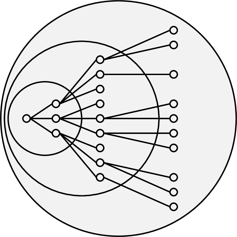
Motivated by this observation, our decomposition \({\cal C}\) will consist of balls \(N(v, 3^{k})\) for some \(v\) and \(k\). For each \(0 \leqslant k \leqslant\log_{\phi} n\), we sample \(S_{k} \subseteq V\) by including each vertex with probability \(p_{k} \sim \phi^{-k}\). Then, for each \(u \in S_{k}\), we add \(N(u, 3^{k})\) to \({\cal C}\) if \(|N(u, 3^{k} + 1)| \leqslant\phi^{k + 1}\). Since \(|S_{k}| = O(n\phi^{-k})\) with high probability, the total time required is at most \(O(\sum_{k} |S_{k}| \phi^{2k + 2}) = O(\sum_{k} n \phi^{k+2}) = n^{2 + o(1)}\).

Above, we have argued that each set has small diameter. Furthermore, since \(|S_{k}| = O(n\phi^{-k})\) with high probability, we have that \(\sum_{u \in S_{k}} |N(u, 3^{k} + 1)| = O(n \phi) = n^{1 + o(1)}\), as desired.

It remains to argue that every vertex \(v \in N(u, 3^{k})\) for some \(N(u, 3^{k}) \in {\cal C}\). Let \(k \geqslant 1\) be the smallest positive integer satisfying \(|N(v, 3^{k})| \leqslant\phi^{k}\) so that \(|N(v, 3^{k - 1})| > \phi^{k - 1}\). Note that such a \(k\) always exists since \(|N(v, 1)| > 1\) unless \(v\) is an isolated vertex. Then, with high probability, some \(u \in S_{k - 1}\) hits \(N(v, 3^{k - 1})\). Then, since \(\mathrm{dist}(u, v) \leqslant 3^{k - 1}\) and \(2 \cdot 3^{k - 1} + 1 \leqslant 3^{k}\), we have \(|N(u, 3^{k - 1} + 1)| \leqslant|N(v, 2 \cdot 3^{k - 1} + 1)| \leqslant|N(v, 3^{k})| \leqslant\phi^{k}\) , resulting in \(N(u, 3^{k - 1})\) being added to \({\cal C}\), as desired.

Note that the above process gives a covering of the vertices. We can obtain a decomposition by removing duplicated vertices from the clusters.

2.4 Extension to Bounded Weights↩︎

Finally, we describe how to extend the algorithm to handle weighted graphs with small integer weights bounded by \(B\). Note that an algorithm that computes MSSP on graphs with integer weights bounded by \(\Theta(B)\) also computes the rectangular \((\min, +)\)-product of two integer matrices with entries bounded by \(B\). Given \(S_{\mathrm{in}} \times n\) matrix \(X\) and \(n \times n\) matrix \(Y\), construct a three-layer graph with \(V_1 = S_{\mathrm{in}}, V_2 = [n], V_3 = [n]\) and edges \((s, u)\) for \(s \in V_1, u \in V_2\) with weight \(10B + X[s, u]\) and edges \((u, v)\) for \(u \in V_2, v \in V_3\) with weight \(10B + Y[u, v]\). Then, \(\mathrm{dist}(s, v) = 20B + (X \star Y)[s, v]\) whenever \((X \star Y)[s,v] < \infty\) and is at least \(40B\) otherwise.

Thus, our goal is to develop an algorithm that runs in \(\mathsf{T}_{\mathrm{MPP}}(|S_{\mathrm{in}}|, n, n \mid B) = \widetilde{O}\left(B\mathsf{T}_{\mathrm{MUL}}(|S_{\mathrm{in}}|, n, n)\right)\) time, where \(\mathsf{T}_{\mathrm{MPP}}(n^{a}, n^{b}, n^{c} \mid B)\) denotes the time required to compute the \((\min, +)\)-product between integer matrices of dimension \(n^{a} \times n^{b} \times n^{c}\) with integer entries bounded by \(B\).

We first describe an \(\hat{O}(B^2 \mathsf{T}_{\mathrm{MUL}}(|S_{\mathrm{in}}|, n, n))\) time algorithm. Treat \(G\) as an unweighted graph, and compute an \((n^{o(1)}, n^{o(1)})\)-low diameter small neighborhood decomposition.

Now, fix a source \(s\). To ensure correctness, in order to compute \(L(s, \mathrm{level}(s) + 1)\) we need two modifications to account for the fact that edge weights can be up to \(B\). We need to (1) consider any cluster \(V_i\) that intersects \(L(s, r)\) for any \(\mathrm{level}(s) - B \leqslant r \leqslant\mathrm{level}(s)\), and (2) compute \(N(V_i) \cap L(s, \mathrm{level}(s) + 1)\) via a \(B\)-bounded \((\min, +)\)-product. Revisiting the analysis of our unweighted algorithm, we obtain a running time of \(\hat{O}(B^2 \mathsf{T}_{\mathrm{MUL}}(|S_{\mathrm{in}}|, n, n))\) since (1) implies that \(V_i\) is relevant to \(s\) for \(Bn^{o(1)}\) iterations (in contrast to \(n^{o(1)}\)), while (2) implies that we must use \(B\)-bounded \((\min, +)\)-products in place of a Boolean product.

To ensure that each cluster is relevant to any source \(s\) only for \(n^{o(1)}\) iterations of the while loop, we instead take the following approach. Consider graphs \(G_{b}\) for \(b \leqslant\log B\) consisting of all edges with weight between \(2^{b}\) and \(2^{b + 1}\). We obtain low diameter small neighborhood decompositions for all \(G_{b}\) as unweighted graphs, denoted \({\cal C}_{b} = \left\{ V_{i}^{(b)} \right\}\). Now, while each cluster \(V_{i}^{(b)}\) has diameter \(2^{b}n^{o(1)}\), we only need to consider cluster edges in \(G_{b}\) incident to \(V_{i}^{(b)}\) for every \(2^{b}\) layers of the shortest path tree from \(s\), since each of these edges has weight at least \(2^{b}\). Our final algorithm for bounded weights selects a cluster that is relevant to many sources, and relaxes all edges of the appropriate weight range incident to this cluster. To ensure correctness and efficiency, we carefully manage which vertices are active for each source and edge weight class, ensuring that the shortest path tree of each source is built accurately (see [thm:bounded-weight-mssp] for details).

2.5 Multiple Source Reachability↩︎

Our algorithm for Multiple Source Reachability (and MSSP on DAGs) employs a simple recursive scheme. Assume that \(G\) is sorted in topological order. Let \(\mathrm{pred}(\pi, v)\) denote the predecessor of \(v\) in path \(\pi\). For any interval \([L, R]\) of \(\ell\) vertices, we employ a recursive scheme \(\textsf{complete}(G, S_{\mathrm{in}}, L, R)\) with the following input/output conditions:

Input: \(\mathrm{reach}(s, v)\) is computed if there is a path \(\pi\) from \(s \in S_{\mathrm{in}}\) to \(v \leqslant R\) where \(\mathrm{pred}(\pi, v) \leqslant L\).

Output: \(\mathrm{reach}(s, v)\) is computed for all \(s \in S_{\mathrm{in}}\) and \(v \leqslant R\).

Our Multiple Source Reachability algorithm computes \(\textsf{complete}(G, S_{\mathrm{in}}, 0, |V|)\). In this overview, we describe how to compute \(\textsf{complete}(G, S_{\mathrm{in}}, L, R)\). Let \(M = (L+R)/2\) be the midpoint of the interval. Note that we can compute \(\textsf{complete}(G, S_{\mathrm{in}}, L, M)\) since the input condition is satisfied. Our goal is to satisfy the input condition of \(\textsf{complete}(G, S_{\mathrm{in}}, M, R)\) which would satisfy the output condition of \(\textsf{complete}(G, S_{\mathrm{in}}, L, R)\). To do so, we need to ensure \(\mathrm{reach}(s, v)\) is computed for any path \(\pi\) from \(s\) to \(v\) with \(L \leqslant\mathrm{pred}(\pi, v) \leqslant M\). We can do this with a single computation of BMM by constructing matrix \(X\) as a \(S_{\mathrm{in}} \times [L, M]\) containing \(\mathrm{reach}(s, u)\) for \(u \in [L, M]\) and a matrix \(Y\) as a \([L, M] \times [M, R]\) submatrix of the adjacency matrix, ensuring that all paths passing through \([L, M]\) are accounted for. The running time of the recursion is thus \[T(\ell) = 2 T(\ell/2) + \mathsf{T}_{\mathrm{BMM}}(S_{\mathrm{in}}, \ell, \ell)\] which yields \(\mathsf{T}_{\mathrm{BMM}}(S_{\mathrm{in}}, n, n)\) by appealing to the root-heavy case of the Master Theorem. Our algorithm for MSSP on DAGs employs a similar recursive structure, replacing each BMM instance with an appropriate Min-Plus Product.

3 Preliminaries↩︎

Let \([n] = \left\{ 1, \dots, n \right\}\). Let \(\log\) denote the base-2 logarithm, unless stated otherwise. For any set \(S\), let \(|S|\) denote the size of the set. For an empty set, we use the conventions \(\min(\emptyset) = \infty\) and \(\max(\emptyset) = - \infty\). In our algorithms, we use \(x \overset{+}{\gets}y\) to denote \(x \gets x + y\) and \(x \overset{\min}{\gets}y\) to denote \(x \gets \min(x, y)\). For sets, we use \(A \overset{\cup}{\gets}B\) to denote \(A \gets A \cup B\).

For a graph \(G = (V, E)\), we typically use \(n = |V|\) and \(m = |E|\) to denote the number of vertices and edges respectively. We use \(G = (V, E, \mathrm{wt})\) to denote a weighted graph with weight function \(\mathrm{wt}: E \mapsto {\mathbb{Z}}\). For any \(S \subseteq V\), \(E(S)\) denotes all edges incident to some vertex in \(S\). Unless otherwise stated, all graphs are undirected. Furthermore, we assume (without loss of generality) that all graphs are connected.

For any two vertices \(s, t \in V\), let \(\mathrm{dist}_{G}(s, t)\) denote the length of the shortest path from \(s\) to \(t\). When the context is clear, we omit \(G\) and write \(\mathrm{dist}(s, t)\). For any path \(\pi \subseteq G\) (not necessarily shortest), let \(|\pi|\) denote the length, or number of edges, of \(\pi\). For a subset of vertices \(S \subseteq V\) and a vertex \(v \in V\), let \(\mathrm{dist}(S, v) := \min_{s \in S} \mathrm{dist}_{G}(s, v)\). For any vertex \(s \in V\), let \(N(s, r) := \left\{ v \textrm{ s.t. }\mathrm{dist}(s, v) \leqslant r \right\}\) and for a subset of vertices \(S \subset V\), let \(N(S, r) := \left\{ v \textrm{ s.t. }\mathrm{dist}(S, v) \leqslant r \right\}\). Let \(N(v) := N(v, 1)\) and \(N(S) := N(S, 1)\). Let \(\mathrm{diam}_{G}(S) := \max_{s, t \in S} \mathrm{dist}_{G}(s, t)\) denote the diameter of a subset \(S\). For a given vertex \(s \in V\) and distance \(r\), let \(L(s, r) := \left\{ v \textrm{ s.t. }\mathrm{dist}(s, v) = r \right\}\).

Given a matrix \(A\), we let \(A[i, j]\) denote the entry of \(A\) in the \(i\)-th row and \(j\)-th column. Let \(0_{a \times b}\) denote an \(a \times b\) matrix of \(0\)s. Let \(\mathsf{T}_{\mathrm{MUL}}(n_1, n_2, n_3)\) denote the time required to compute a \(n_1 \times n_2 \times n_3\) dimensional matrix product i.e. the product of an \(n_1 \times n_2\) matrix and an \(n_2 \times n_3\) matrix. Given matrices \(A, B\), we let \(AB\) denote the standard matrix product (either Boolean or integer), and \(A \star B\) the \((\min, +)\) (or Min-Plus) matrix product, where \((A \star B)[i,j] = \min_{k} \{A[i,k] + B[k,j]\}\). Let \(\mathsf{T}_{\mathrm{BMM}}(n_1, n_2, n_3)\) denote the time required to compute a \(n_1 \times n_2 \times n_3\) dimensional boolean matrix product, and \(\mathsf{T}_{\mathrm{MPP}}(n_1, n_2, n_3 \mid B_1, B_2)\) the time required to compute the \((\min, +)\) product of a \(n_1 \times n_2\) matrix with entries in \([B_1] \cup \left\{ \infty \right\}\) and a \(n_2 \times n_3\) matrix with entries in \([B_2] \cup \left\{ \infty \right\}\). Let \(\mathsf{T}_{\mathrm{MPP}}(n_1, n_2, n_3 \mid B) := \mathsf{T}_{\mathrm{MPP}}(n_1, n_2, n_3 \mid B, B)\). In some cases, we write \(\mathsf{T}_{\mathrm{BMM}}(A, B, C) := \mathsf{T}_{\mathrm{BMM}}(|A|, |B|, |C|)\) where \(A, B, C\) are sets. We also allow combinations of sets and integers, e.g. for set \(A\) and integers \(n_2, n_3\), \(\mathsf{T}_{\mathrm{BMM}}(A, n_2, n_3) := \mathsf{T}_{\mathrm{BMM}}(|A|, n_2, n_3)\).

4 Low Diameter Small Neighborhood Decomposition↩︎

In this section, we present an efficient algorithm for computing a low diameter small neighborhood decomposition. We begin by defining the desired properties.

We now give an efficient algorithm for computing a low diameter small neighborhood decomposition.

From our above theorem, we obtain a specific decomposition.

We remark that by appropriately setting parameters, we can obtain a low diameter small neighborhood decomposition where exactly one of the diameter and expansion factor is polylogarithmic and both are sub-polynomial. However, for our applications, it suffices to obtain a decomposition where both are sub-polynomial.

5 Undirected Multiple Source Shortest Paths↩︎

In this section, we present our algorithms for MSSP in undirected graphs.

5.1 Undirected Unweighted Multiple Source Shortest Paths↩︎

We begin with our algorithm for undirected, unweighted graphs.

Combined with [cor:boundary-decomposition], we prove our main result.

We prove [thm:mssp-reduction] in the remainder of 5.1. Consider the following procedure.

5.2 Extension to Bounded Weights↩︎

We now extend our algorithm to handle undirected graphs with small integer weights.

Note that it is without loss of generality that we assume all weights are positive: a negative edge in undirected graphs creates a negative cycle, and all pairwise distances become \(-\infty\) (recall we assume the graph is connected). Also, any vertices joined by a weight \(0\) edge can be merged and treated as one vertex. Assume without loss of generality that \(B\) is a power of \(2\). We will require a simple generalization of bounded Min-Plus products.

We are now ready to prove [thm:bounded-weight-mssp]. Consider the following procedure which for presentation we break into an initialization phase and a computation phase. In the initialization phase, we decompose the graph and initialize various useful data structures.

In the computation phase, we use the computed decompositions and data structures to compute shortest paths.

We prove the remaining lemmas. We begin with a few useful claims.

We are ready to prove the required lemmas.

5.3 Applications↩︎

We give some applications of our MSSP algorithm.

5.3.1 Hop-Set Construction↩︎

Our first application is the first non-trivial algorithm for explicitly constructing hop-sets.

We give an efficient algorithm for computing exact \(\beta\)-hop-sets on dense graphs, improving upon the known \(\min\left( n^3/\beta, n^{\omega} \right)\) time algorithm.

5.3.2 Additive Emulator Construction↩︎

We give a simple, efficient algorithm for constructing a \(+4\)-emulator on undirected graphs.

6 Reachability and Shortest Paths on Directed Graphs↩︎

We give a simple recursive scheme that obtains optimal running time for directed reachability.

In fact, our algorithm, with minor modifications, can be used to compute MSSP on unweighted directed acyclic graphs.

We in fact prove a slightly stronger result.

[thm:dag-mssp] follows by applying \(B = 1\) and \(D = n\).

6.1 Application: Shortcut Sets↩︎

We give our improved algorithm for computing shortcut sets of linear size. Recall that for a directed graph \(G\), \(\mathrm{TC}(G)\) denotes the transitive closure of \(G\) and \(\mathrm{diam}(G)\) is the maximum of \(\mathrm{dist}(u, v)\) over \((u, v) \in \mathrm{TC}(G)\).

We give a faster algorithm for computing shortcut sets.

We remark that using our algorithm for Multiple Source Reachability, one can achieve a running time of \(\mathsf{T}_{\mathrm{BMM}}(n/D, n, n)\). However, 12 is at least as fast for all \(D = O(\sqrt{n})\).

7 Min-Plus Product with Distinct Entry Bounds↩︎

In this appendix, we discuss lower bounds for directed MSSP from Min-Plus Matrix Multiplication. We begin with the lower bound given in 2 .

There are several known algorithms for computing \(\mathrm{MPP}(n_1, n_2, n_3 \mid B_1, B_2)\):

1. We can compute \(\mathrm{MPP}(n_1, n_2, n_3 \mid \max(B_1, B_2))\) in time \(\widetilde{O}\left(\max(B_1, B_2) \mathsf{T}_{\mathrm{MUL}}(n_1, n_2, n_3)\right)\) [15].

2. [29] showed that (see Lemma B.2 of [29]) if \(B_1 \leqslant B_2\), then \[\mathsf{T}_{\mathrm{MPP}}(n_1, n_2, n_3 \mid B_1, B_2) = \tilde{O}\left(\min_{1 \leqslant t \leqslant n_2 n_3} \mathsf{T}_{\mathrm{MPP}}\left(n_1, n_2, \frac{n_2n_3}{t} \mid B_1 \right) + t n_1 n_3\right) \text{.}\] Similarly, if \(B_2 \leqslant B_1\), then \[\mathsf{T}_{\mathrm{MPP}}(n_1, n_2, n_3 \mid B_1, B_2) = \tilde{O}\left(\min_{1 \leqslant t \leqslant n_1 n_2} \mathsf{T}_{\mathrm{MPP}}\left(\frac{n_1 n_2}{t} , n_2, n_3 \mid B_2 \right) + t n_1 n_3\right) \text{.}\]

We give a simple algorithm that beats the above two algorithms in certain regimes of parameters.

4 compares the running time of our directed MSSP algorithm ([thm:dag-mssp]), the directed MSSP algorithm of [56], and the best known algorithms for computing 2 .

References↩︎

---

1. Supported by NSF HDR TRIPODS Phase II grant 2217058 (EnCORE Institute).↩︎

2. Throughout this paper, we consider dense graphs with \(m = O(n^2)\).↩︎

3. \(\omega \le 2.372\) [14] is the fast matrix multiplication exponent, or the smallest constant \(c\) such that an \(n \times n \times n\) matrix product can be computed in \(n^{c+o(1)}\) time. \(\widehat{O}\) hides sub-polynomial factors.↩︎

4. Our equivalence holds under the mild assumption that \(\mathsf{T}_{\mathrm{BMM}}(2m, 2n, 2n) \geqslant 4 \mathsf{T}_{\mathrm{BMM}}(m, n, n)\) for all \(m, n \geqslant 1\). Note that this assumption essentially requires that \(\mathrm{BMM}\) scales at least linearly with input size. We remark that our improved running time holds regardless of the assumption. See proof of 3 for details.↩︎

5. Let \(A\) be an \(s \times n\) matrix and \(B\) an \(n \times n\) matrix. We build a three layered graph with vertex layers \(V_1, V_2, V_3\), where \(|V_1| = s\), \(|V_2| = |V_3| = n\), encode \(A\) into \(V_1 \times V_2\) (i.e., there is an edge if the corresponding entry of \(A\) is \(1\), and no edge otherwise) and \(B\) into \(V_2 \times V_3\), and note that for \(i \in V_1, j \in V_3\), \(\mathrm{dist}(i, j) = 2\) if and only if \((AB)[i, j] = 1\).↩︎

6. Like [cor:mssp], the equivalence holds under the mild assumption that \(\mathsf{T}_{\mathrm{MPP}}(2m, 2n, 2n \mid B) \geqslant 4 \mathsf{T}_{\mathrm{MPP}}(m, n, n \mid B)\) for all \(m, n \geqslant 1\). As before, our improved running time holds regardless of the assumption.↩︎

7. \(\omega(a, b, c)\) is the rectangular matrix multiplication exponent, or the smallest constant \(d\) such that an \(n^{a} \times n^{b} \times n^{c}\) matrix product can be computed in \(n^{d+o(1)}\) time.↩︎

8. Their algorithm is actually more general and can be used to solve multiple-source multiple-target shortest paths.↩︎

9. To avoid confusion, we call our decomposition a low diameter small neighborhood decomposition.↩︎