Forget, Anticipate and Adapt: Test Time Training for Long Videos
June 25, 2026
Abstract
Test Time Training (TTT) is a mechanism in which a model adapts to an incoming test-sample by performing some self-supervised (SSL) task and updating its weights even during inference. This procedure does not require labels at test-time. This paper
focuses on TTT for long-videos. A major concern with existing approaches is: 1) they perform TTT updates using a sliding window containing frames in the past, whose compute increases linearly with the size of window. This becomes computationally
intractable when the videos are hours long. 2) TTT is performed even when temporally close frames look similar, thereby consuming a lot of compute.
We present the Frame Forgetting Network (FFN) that: 1) operates on only three frames within the sliding window, namely the frame that exits, the current frame and the frame after that. The model still manages to retain temporal context and work for hours
long-videos; 2) mathematically define a ‘surprise’ metric: how much ‘new information’ the incoming frame contains with respect to the past seen frame. This facilitates determining how to modify the effective window size during TTT and constitutes the core
mechanism of an adaptive windowing algorithm. Additionally, we curate a dataset EpicTours containing up to 3 hour long videos of walking city-tours, whereas earlier datasets on this problem were only 5 min long. We demonstrate FFN’s empirical effectiveness
on dense-segmentation, video classification tasks, generalization to depth-estimation, and multi-hour long videos. The project page can be found at https://github.com/rajatmodi62/ffn.
1 Introduction↩︎
Typically, machine learning models only update their weights during training, but freeze them during inference[1], [2]. However, as humans, we possess the ability to continuously learn and adapt to our ever-changing environment. Test Time Training (TTT) shows
the promise of bringing a similar adaptive capability to artificial intelligence, allowing a model to continuously learn and update its weights even while testing, entirely without the need for ground-truth labels.
However, applying TTT to video processing presents a unique set of challenges. Existing online distillation methods are based on a student-teacher setup [3], with the teacher usually deployed on a remote server and the student on a local device. However, this is a bottleneck in offline real-world scenarios, such as disaster-prone regions, where server
connectivity may be limited.
Consequently, the key challenge lies in determining how to perform TTT on videos locally, on-device, and computationally cheaply. This is especially critical for dense computer vision tasks, such as segmentation, where each pixel matters, and should
ideally be achieved utilizing a single model.
Historically, there have been two approaches towards adaptation: either (i) train a dedicated video model specifically for the task, or (ii) start from a pre-trained image model and adapt it accordingly. Unfortunately, large-scale pre-training
datasets for video remain limited, and efforts to repurpose image models are inherently constrained by the absence of explicit temporal information. Furthermore, existing TTT methods for videos rely on a sliding window approach[4]. A sliding window serves as a fixed-size temporal buffer that holds a defined number of preceding frames and moves forward step by
step as the video advances. Because the model re-evaluates all frames currently inside this window, it performs a duplicate, highly expensive computation at every single timestep. This redundant computation is far too
prohibitive for long videos, thereby limiting practical deployment
To overcome these limitations, we propose the Frame Forgetting Network (FFN). Our approach is built on the core insight that as the sliding window progresses, only one new frame enters, and one frame exits. Thus, a model only needs to pay the
computational cost of processing these crucial frames instead of recalculating the entire window for every time-step.
Our FFN consists of two core components: a Memory Restoration Mechanism (MRM) and an Adaptive Window Algorithm (AWA). The MRM allows the model to actively ‘forget’ its adaptation on past frames exiting the window and ‘restore’ the model’s original
predicted features using a temporal module. Next, the AWA algorithm can dynamically ‘anticipate’ when adaptation is required, improving the management of computational load. Through extensive experiments across \(11\)
datasets, we validate FFN’s competitive performance on dense segmentation tasks, strong generalization on depth estimation, and ability to learn stable representations during recurrent video-processing.
2 Frame Forgetting Network↩︎
First, we shall talk about our problem statement, cover preliminaries on TTT, and then discuss our Frame Forgetting Network (FFN).
2.1 Problem statement↩︎
Given a streaming long-video \(\mathcal{V}=\{x_1,x_2,x_t,...,x_n\}\), a model can access only the past frames \(x_1,x_2,...,x_{t-1}\), the current frame \(x_t\), but not the future. The problem is focused on adaptation: for \(x_{t}\), how does the model decide when to ‘adapt’ or not. This adaptation should help improve downstream performance and be cheaper to compute. In this work, we focus on adaptation using TTT, an instantiation that allows a model to even update its weights during inference.
2.2 Preliminaries↩︎
TTT involves two phases, a) Training Time Training and b) Test Time Training.
Training Time Training: Fig1 (i) illustrates how a TTT setup works. We consider a model containing backbone \(f\), a downstream head \(h\) and
a self-supervised (SSL) head \(g\) specializing in some task that does not require external labels (e.g., image reconstruction). First, we train \((f,g,h)\) jointly in a train set,
which consists of densely-annotated images. This first phase is known as training-time-training[4].
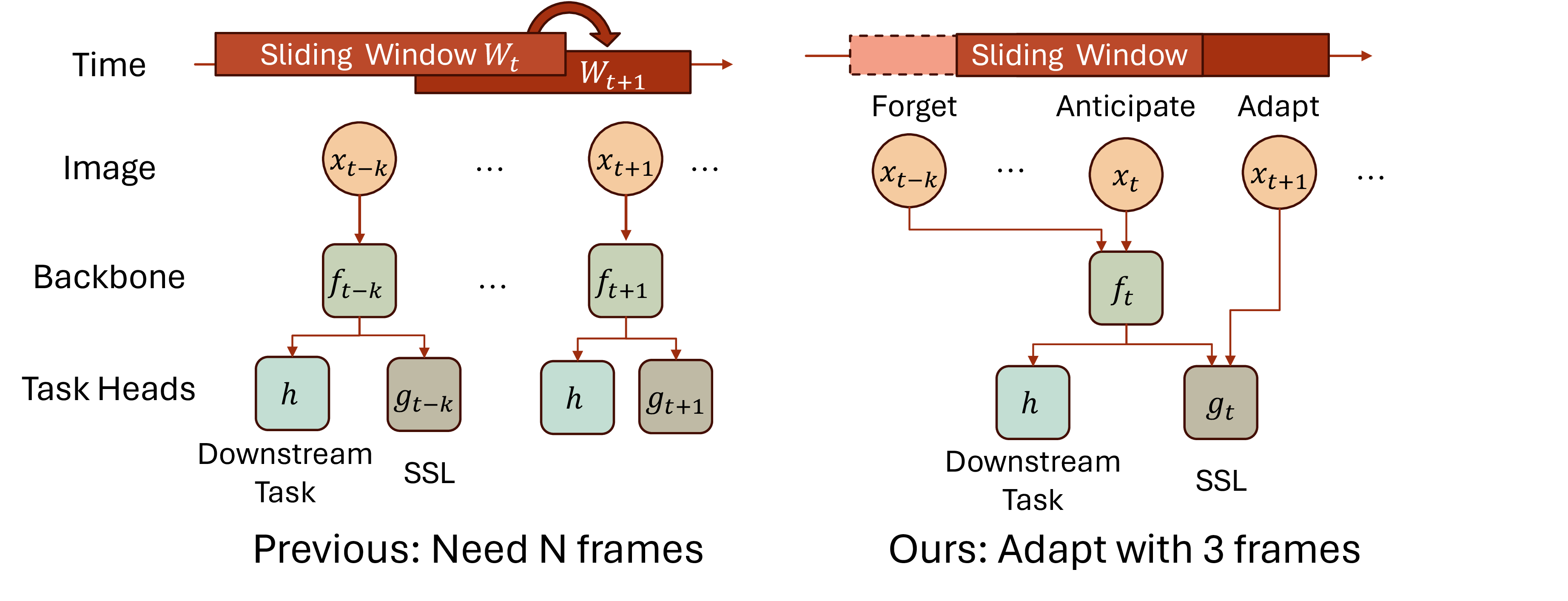
Test Time Training: Here, the model is given access to a test-video consisting of several frames. The model looks at an incoming frame \(x_t\) and tries to reconstruct it. As in Fig1, this involves feed-forwarding \(x_t\) through the backbone \(f\), then through the SSL-head \(g\), thus computing the RGB reconstruction \(x'_t\). Next, we estimate the reconstruction loss \(\ell_{s}(x'_t, x_t)\), where \(x'_t = g{\circ}f(x_t)\). This may be used to update \(f,g\) over several iterations. The downstream head \(h\) is kept frozen throughout. This is known as test-time-training.
2.3 The Principle of locality↩︎
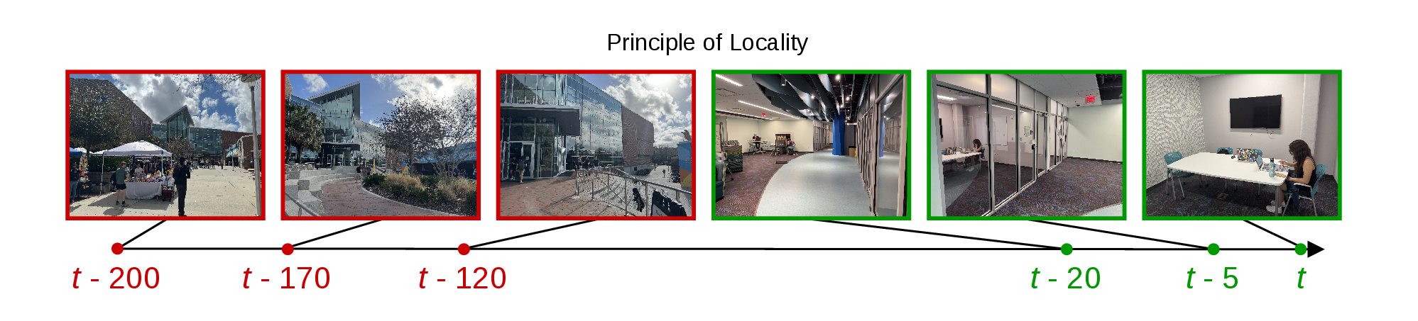
Adaptation in videos follows a ‘principle of locality’[4]. Intuitively, a frame at \(t=1\) (say indoors) may not be relevant to the frame at \(t=5k\) (say outdoors). Consider a current frame \(x_{t}\). Instead of looking at the entire past timesteps, existing TTT methods use a sliding window of size \(k\), which we denote by \(W_{t}\). More formally, the TTT update rule at \(x_t\) is governed by: \[f_{t}, g_{t} = \arg \min_{f,g} \frac{1}{k} \sum_{t'=t-k+1}^{t} \ell_{s}(g \circ f(x_{t}), x_{t}), \label{eq:ssl95update}\qquad{(1)}\] where \(k\) is the size of a window containing frames encountered in the past (illustrated by window \(W_t\) in Fig1). This creates two issues:
The window \(W_t\) sums up the \(k\) past frames for each timestep. Inductively, \(W_t\) slides over time (e.g., \(W_{t+1}\)) with the model’s weights being reset after every update. The arg min operator requires backpropagation through \(f,g\) every timestep \(t\). Thus, TTT quickly becomes computationally intractable, with a \(2hr\) video (\(7200\) frames) taking up to \(8hrs\).
The model wastes a lot of compute; for example, it shall perform TTT even when two successive frames are pixel-wise identical.
Note that \(f,g\) can change their weights over time as the model undergoes adaptation. We denote this by the subscript \(t\), namely \(f_t\), and \(g_t\).
2.4 Method↩︎
The sliding window-invariant: Consider a sliding window \(W_{t} = [x_{t-k}, x_{t-k+1},
\\...,x_{t-1}, x_{t}]\), and the next window \(W_{t+1}=[x_{t-k+1},...,x_{t},x_{t+1}]\). Mathematically, this reveals that both have the same number of frames except for two: frame numbered
\(x_{t-k}\) that exits the window \(W_{t+1}\) and frame numbered \(x_{t+1}\) that enters the window \(W_{t+1}\).
The intuition that operating on sliding windows requires a mechanism to update a running state and only handle elements which come in/go out is well-known in data structures like arrays (e.g., Kadane’s Algorithm [5]). However, inducing such behavior is non-trivial in neural nets, which in-principle may be treated as forms of parallel distributed
memories[6].
This reveals that while making a transition from \(W_{k}\rightarrow W_{k+1}\), we don’t need to process \(k\) frames. Rather, we can operate on only \(3\) frames by defining three mechanisms:
Forget: for frame \(x_{t-k}\), ‘forget’ the model’s features after adaptation, and ‘restore’ the model’s predicted features to those prior to TTT.
Anticipate: The current frame \(x_{t}\) under processing can be used to ‘anticipate’ what shall come next at \(x_{t+1}\). For brevity, we call this prediction \(x'_{t+1}\)
Adapt: Compare \(x'_{t+1}\) with the actual frame \(x_{t+1}\). If the difference is greater than some threshold \(\tau\), the model chooses to adapt on \(x_{t}\). Otherwise, it can perform simple inference on \(x_{t}\) and move on. Note that inference is equivalent to the feed-forward \(f\circ h(x_t)\) through the model.
An initial approach might be to hard-code \(\tau\) to some value (say \(0.5\)). However, this makes the model’s behavior static: there might be some consecutive frames
who have large pixel-difference, but do not deserve adaptation (for e.g., slight rotation of images of the same object). Thus, we need a mechanism that could govern this \(\tau\) dynamically.
Inspired by this, we present the Frame Forgetting Network (FFN). It consists of two components: 1) Memory Restoration Mechanism (MRM) 2) Adaptive Window Algorithm (AWA). MRM allows the model to
‘forget’ the frame that moves out of the window (\(x_{t-k}\)), while AWA allows the model to anticipate if \(x_{t}\) deserves adaptation, by dynamically estimating \(\tau\). Next, we explain these blocks.
2.5 The Memory Restoration Mechanism (MRM)↩︎
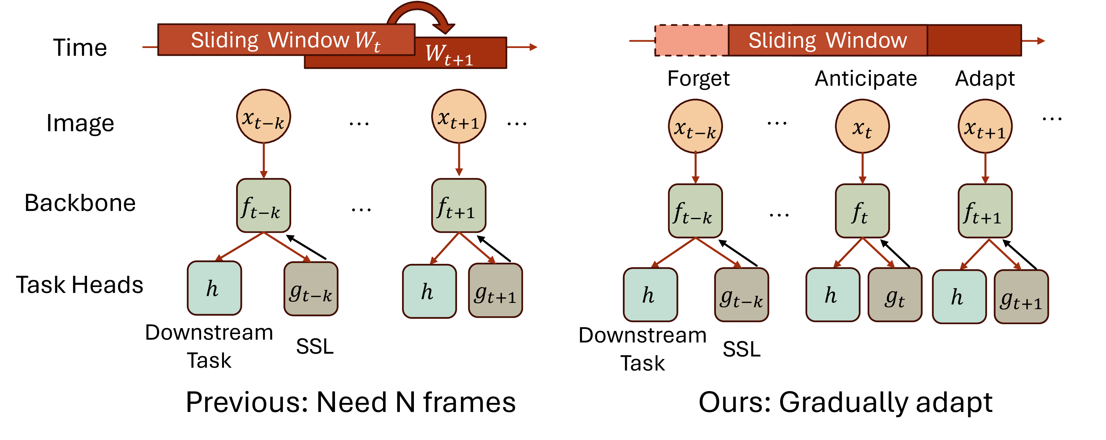
To forget the model’s adaptation on \(x_{t-k}\), we can first cache its features before adaptation; i.e., we estimate \(f_{t-k-1}(x_{t-k})\). The idea is that the
current weights of the model \(f_t\) should be adjusted so that it can predict the earlier features \(f_{t-k-1}(x_{t-k})\). This suggests that the model \(f\) requires two things: i) input \(x_{t-k}\), and ii) a sense of time \(t-k\). We propose instilling this via a temporal module.
We implement a temporal module as a three layered MLP1. First, the timestep \(t-k\) corresponding to \(x_{t-k}\) is injected into the temporal module. Instead of conditioning the temporal module by a single integer, we implement \(t\) as a one-dimensional positional encoding, similar to the one
used in transformers[8]. Note that injecting time \(t\) in an image-based backbone \(f\) may be cheaper than training a video-backbone from scratch. The output of temporal module is then used to condition the backbone \(f_{t-k-1}\), resulting in two input arguments \(x_{t-k},t-k\). Mathematically, we can minimize the following: \[\ell = f_t(x_{t-k},t-k) - f_{t-k-1}(x_{t-k}, t-k)\] This can be used to make a single gradient step through backpropagation and
adjust the weights of the backbone \(f\).
2.6 Adaptive Window Algorithm (AWA)↩︎
An Anticipative Head: Given the current frame \(x_{t}\), we need to anticipate whether adaptation is required. The idea is to allow the model to take \(x_{t}\)
as input, predict the next frame \(x_{t+1}'\), and compare with the real frame \(x_{t+1}\). The average of pixel-wise difference can then serve as an indicator if adaptation is
required2. Thus, we define the visual space difference as \[ v_{visual}(t) = \frac{2}{\sqrt{h\times w}}
\sum_{h,w} \frac{\|x_{t+1} - x_{t+1}'\|_2}{255}
\label{eq:v95visual}\tag{1}\] One concern about equation 1 is that if an incoming frame \(x_{t+1}\) just ‘rotates’ slightly over the current frame \(x_{t}\), \(v_{visual}\) shall be very high owing to the fluctuations in the pixel space (for e.g., capturing a video over phone). Intuitively, however, these two frames still look
almost the same. This means that low-level information might not be a reliable indicator.
Thus, we make use of the following observation: higher layers of a model \(f\) remain invariant to minor-changes in input frames. Inspired by this, we define a memory buffer \(B=[v_{latent}(t_1), v_{latent}(t_2), ...,v_{latent}(t_{last})]\), where \(v_{latent}(t_i) = f_{t_{i}}(x_{t_i})\). Note that different \(t_{i}\) here denote the
timesteps when the model actually ‘adapted’ in the past, and need not be consecutive. The idea is that if the \(latent\) feature of the most recently adapted past frame (\(t_{last})\) is very similar to the latent feature of the current frame \(x_t\), we must not adapt. Please note that \(t_{last}\) need not be
equal to \(t-1\). We define an anticipation matrix A as:
\[A = \frac{v_{latent}(t_i) \cdot v_{latent}({t_{last}})}{\|v_{latent}(t_i)\|_2 \|v_{latent}({t_{last}})\|_2} \label{eq:f95latent}\qquad{(2)}\]
The surprise metric: Both equations 1 and ?? can be unified together to define a metric that measures how much new information (surprise \(S\)) a frame \(x_{t}\) provides to the model. We define \(S\) as: \[S_t = \left[ \log(1 + v_{\text{visual}}(t)) \right] \times [1 - A]\] Next, we consider three cases: (a)
when video contains static frames (e.g., CCTV camera feed): Here \(v_{visual}\approx 0, A\approx 1\), so surprise \(S_t \approx 0\); (b) when video contains a shaking camera (e.g., person
captures a video with a head-mounted display): Here the scene remains the same, but frames change a lot. Therefore \(v_{visual}\uparrow\), \(A\approx constant\), so surprise \(S_t\) stays low ; (c) jump cuts, where the scene changes suddenly (say a transition from indoors to outdoors). There \(v_{visual}\uparrow\), \(A\uparrow\), however \(v_{visual}\) increases far more than \(A\)3, so
surprise \(S_{t}\) takes on a very high value.
Both cases b) and c) suggest that if \(S_{t}\) exceeds or equals to some adaptive threshold \(\tau_t\), the model should perform TTT. Otherwise, it may perform inference on the
frame \(x_t\) (i.e., a single forward pass \(h(f_{t-1}(x_t))\)) and move on to the next frame \(x_{t+1}\). In this case, \(f_{t}=f_{t-1}\), since it is not updated. Next, we derive \(\tau_t\).
Deriving the adaptive threshold \(\tau_t\): Recall that the buffer \(B\) contains latent features of all frames on which TTT was performed. We assume that the size
of this buffer is \(N\). Each element in the buffer contains the latent feature \(v_{latent}(t_i)\), and the surprise computed at \(t_{i}\). We define \(\tau_t\) as : \[\mu_{t} = \frac{1}{W} \sum_{i=t-W}^{t-1} S_{i} \quad ; \quad \sigma_{t} = \sqrt{\frac{1}{W} \sum_{i=t-W}^{t-1} (S_{i} - \mu_{t})^{2}}
\label{eq:running95avg}\tag{2}\] \[\tau_{t} = \mu_{t} + \sigma_{t}\] Intuitively, \(\mu_t\) tracks how the mean of surprise flows over time[11], [12], \(\sigma_t\) estimates variance, \(\tau_t\) is one standard deviation away from the mean4. Note that while the size of buffer \(N\) is fixed, the
threshold \(\tau_t\) itself is dynamic. Therefore, unlike equation ?? where TTT was done for each iteration, the model now dynamically decides when to do TTT. Also, we are processing three frames in a timestep and
not N.
Revisiting the cold-start problem: Initially, our model does not see any frame, hence the buffer \(B\) is empty. Therefore, it is difficult to make a reliable estimate of whether to adapt or not. This issue
also appears as a cold-start problem in recommendation systems[13]. We attempt to resolve this by ‘adapting’ \(B\) initial-frames until the buffer is full. Since \(W<<<\) video-length, this approach worked quite well, albeit at the expense of some initial-lag in the system5.
3 Experiments on FFN↩︎
Here, we experiment with FFN across a wide range of benchmarks, for example, (i) dense tasks like semantic, instance, and panoptic segmentation; (ii) generalization across video depth-estimation; (iii) action-classification; (iv) segmentation on
multi-hour long videos.
Datasets: We report video segmentation results in COCO-Videos[4], KITTI-STEP[14]. For action classification, we report UCF101[15], Something-Something v2[16]. Similarly, for depth-estimation, we create a similar setup as Video-DepthAnything (CVPR’2025)[17], and show results on \(6\) datasets (KITTI[18], Scannet[19], Bonn[20], NYUv2[21], Sintel[22]). As shown in Table 2, most of these datasets contain only videos up to \(5 mins\) long.

To address this, we propose a new video segmentation dataset, EpicTours Dataset, which contains multi-hour-long videos of people exploring cities across the globe, representing geographical diversity. Our videos are densely annotated
with the help of SAM 3 inference [23], manually filtered/refined by expert human annotators. Notably, our EpicTours dataset contains videos up to
3 hours long, with \(30\) classes (subset of COCO). This enables us to study the applicability of our FFN on real-world scenarios, for example, videos containing multiple-people. Please refer to the supplementary for more
details.
| Setting | Method | COCO Videos | KITTI-STEP | |||
|---|---|---|---|---|---|---|
| 3-4 (lr)5-7 | Inst.\(\uparrow\) | Pan.\(\uparrow\) | Val.\(\uparrow\) | Test\(\uparrow\) | Time\(\downarrow\) | |
| Independent frames | Main Task Only | 16.7 | 13.9 | 53.8 | 52.5 | 1.8 |
| MAE Joint Training | 16.5 | 13.5 | 53.5 | 52.5 | 1.8 | |
| TTT-MAE No Memory | 35.4 | 20.1 | 53.6 | 52.5 | 3.8 | |
| Full Video | Offline TTT-MAE All Frames | 33.6 | 19.6 | 53.2 | 51.2 | 1.8 |
| Stream | LN Adapt | 16.5 | 14.7 | 53.8 | 52.5 | 2.0 |
| Tent | 16.6 | 14.6 | 53.8 | 52.2 | 2.8 | |
| Tent w/ Class Bal. | 16.7 | 14.8 | 53.8 | 52.5 | 3.7 | |
| Self-Train | - | - | 54.7 | 54.0 | 6.6 | |
| Self-Train w/ Class Bal. | - | - | 54.1 | 53.6 | 6.9 | |
| Online TTT-MAE (n.o. s.w.) | 35.3 | 20.8 | 48.1 | 51.7 | 0.4 | |
| Online TTT-MAE (s.w.) | 37.6 | 21.7 | 55.4 | 54.3 | 4.1 | |
| 2-7 | FFN (Ours)\(^\dagger\) | 45.1 | 29.6 | 57.3 | 59.5 | 0.7 |
Metrics: For instance, panoptic and semantic segmentation we report Average Precision (AP), Panoptic Quality (PQ), and mIoU respectively. Similarly, for video-depth estimation, we report AbsRel:Absolute Relative Error, and \(\delta_1\) which denotes \(\%\) of pixels where the ratio between the prediction and the ground truth falls below a threshold of \(1.25\). For
action-classification, we report top-1 accuracy.
| Video Dataset | Len (s) \(\uparrow\) | Frames\(\uparrow\) |
|---|---|---|
| CityScapes [24] | 1.8 | 3k |
| DAVIS [25] | 3.5 | 3.4k |
| YouTube [26] | 4.5 | 123k |
| KITTI-S [27] | 40.0 | 8k |
| COCO-V | 309.0 | 30k |
| EpicTours | 5300.4 | 2.49M |
r0.35
Implementation details: For segmentation (Tab1, Tab[tbl:tab:epic95tour95results]), we initialize the backbone \(f\) with Mask2former, SSL-task head \(g\) from scratch. We train \(g\) jointly during the training-time phase on both image datasets / a single long video. Similarly, \(h\) the task-specific head (segmentation) utilizes Mask2former’s pre-trained weights. For
depth-estimation (Tab3), we leverage the Video-Depth Anything architecture. For video-classification (Tab¿tbl:tab:classification?), we adopt the self-supervised backbone (DINOv3)[28] backbone (a very-recent foundational model). We set the memory buffer size \(W=50\), perform a
single gradient step per incoming-frame, and use the Adam optimizer. Our SSL-head \(g\) is trained with next-frame anticipation instead of current-frame reconstruction. We perform experiments with \(3\) seeds and report their mean accuracy. All experiments are performed on a single ampere of 80 GB.
Baselines: Inspired by [4], we consider multiple baselines that span image-models, offline video processing,
test-time-adaptation (TTA), test-time-training. In 1, we categorize our baselines as (i) independent frames: the main task only means zero-shot per-frame inference on a model trained on image-segmentation. MAE
joint-training jointly pretrains MAE[29] for reconstruction/segmentation. Similarly, TTT-MAE memory takes the previous MAE-joint training baseline,
performs TTT on each frame independently (ii) full-video: an ideal offline-oracle, allowed to access the entire video (iii) stream: a tougher setup where a model only encounters frames one-by-one, ‘without’ peeking in
the future.
Our TTA baselines include the pioneering TENT approach[30], layer-norm adaptation, self-training with confident pseudo-labels (to rule out whether
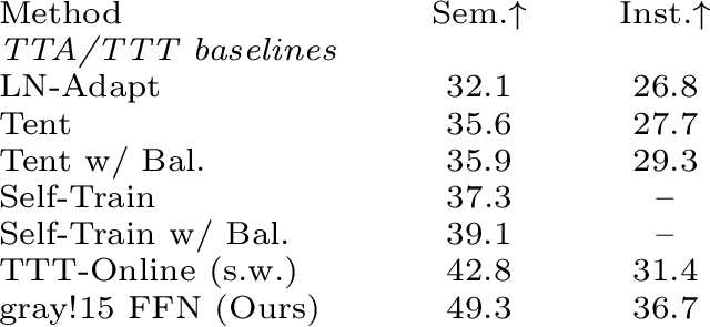
improvements are due to self-supervision or TTT on videos). Next, we consider the TTT-Online baseline [4] across two setups (a) without sliding
window: we perform TTT on a window of \(w\) frames and then move onto a non-overlapping window; (b) with overlapping sliding window: the original setup in [4]. Finally, we consider zero-shot foundational models like DinoV3, evaluating feature robustness on general representation-learning.
FFN can surpass TTT-online on segmentation: In Tab 1 for the COCO-Videos dataset, our FFN obtains \(45.1 (+7.5\uparrow)\) for instance segmentation, \(29.6\) \((+7.9\uparrow)\) for panoptic segmentation. Similarly, on the KITTI-STEP validation set, FFN gets \(57.3 (+1.9\uparrow)\), \(59.5(+5.2\uparrow)\) on the testing split. One takeaway is that the streaming baselines (including our FFN) can surpass the offline TTT-MAE oracle, which can access entire video, thereby validating
the principle-of-locality. Similarly, FFN performs competitively with TTA baselines like Tent.
| Method / Metrics | KITTI [18] | Scannet [19] | Bonn [20] | NYUv2 [21] | Sintel [22] \(^\dagger\) | Scannet \(^\ddagger\) | |||||
|---|---|---|---|---|---|---|---|---|---|---|---|
| 2-3 (lr)4-5 (lr)6-7 (lr)8-9 (lr)10-11 (lr)12-12 | AbsRel (↓) | \(\delta_1\) (↑) | AbsRel (↓) | \(\delta_1\) (↑) | AbsRel (↓) | \(\delta_1\) (↑) | AbsRel (↓) | \(\delta_1\) (↑) | AbsRel (↓) | \(\delta_1\) (↑) | TAE (↓) |
| Zero-shot baselines | |||||||||||
| DAv2-L [31] | 0.137 | 0.815 | 0.150 | 0.768 | 0.127 | 0.864 | 0.094 | 0.928 | 0.390 | 0.541 | 1.140 |
| NVDS [32] | 0.233 | 0.614 | 0.207 | 0.628 | 0.199 | 0.674 | 0.217 | 0.598 | 0.408 | 0.464 | 2.176 |
| NVDS + DAv2-L | 0.227 | 0.617 | 0.194 | 0.658 | 0.191 | 0.700 | 0.184 | 0.679 | 0.449 | 0.503 | 2.536 |
| ChronoDepth [33] | 0.243 | 0.576 | 0.199 | 0.665 | 0.199 | 0.665 | 0.173 | 0.771 | 0.192 | 0.673 | 1.022 |
| DepthCrafter [34] | 0.164 | 0.753 | 0.169 | 0.730 | 0.153 | 0.803 | 0.141 | 0.822 | 0.299 | 0.695 | 0.639 |
| DepthAnyVideo [35] | - | - | - | - | - | - | - | - | 0.405 | 0.659 | 0.967 |
| Video Depth-Anything [36] | 0.083 | 0.946 | 0.087 | 0.933 | 0.070 | 0.961 | 0.064 | 0.967 | 0.300 | 0.633 | 0.570 |
| TTT baselines | |||||||||||
| Online TTT-MAE (s.w.) | 0.071 | 0.958 | 0.076 | 0.949 | 0.064 | 0.970 | 0.058 | 0.974 | 0.265 | 0.710 | 0.495 |
| FFN (Ours) | 0.059 | 0.972 | 0.062 | 0.965 | 0.051 | 0.982 | 0.049 | 0.988 | 0.230 | 0.762 | 0.380 |
FFN for performing TTT with better compute-accuracy tradeoffs: One concern about TTT is that it involves backpropagation through both backbone \(f\), SSL-head \(g\), for
every incoming frame, making it slow in practice. For example, as shown in Tab1, TTT-Online takes \(4.1sec\) per frame. Fortunately, FFN processes only
\(3\) frames per window and consumes \(0.7sec\) per timestep. It also gets a higher result (\(45.1\) vs \(37.6\)) showing a
better compute-accuracy tradeoff. We acknowledge the potential to make TTT even faster.
FFN can generalize to video depth-estimation: We test the generalization ability of FFN on a challenging video depth-estimation task (Table 3). In particular, FFN performs well across the board on
all \(6\) datasets.
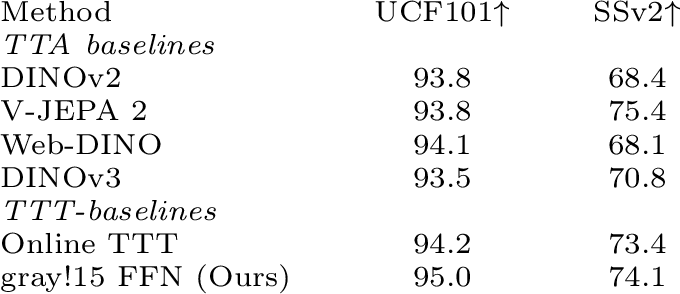
FFN can classify coarse-actions in videos: While segmentation only tests per-frame fine-grained understanding, we also study how well FFN understands the temporal aspect. Thus, we subject FFN to action-classification in UCF101/
Something-Somethingv2. We notice gains of \(0.8\uparrow\), \(0.7\uparrow\), respectively. Note that SSv2 is especially challenging; it requires FFN to reason about direction of
time: e.g., moving something up vs down.
FFN’s effectiveness on realistic hours long videos: In Tab[tbl:tab:epic95tour95results], we subject our FFN
to an even tougher task: how well can it adapt to hours long videos captured in the real-world, often on low-resolution devices like cellphones. In the EpicTours dataset, FFN shows promising gains of \(6.5\%\uparrow\) for semantic segmentation, \(5.3\%\uparrow\) for instance segmentation. A use-case may be to deploy FFN on drones for disaster-relief efforts or food-delivery.
4 Ablations on FFN↩︎
Here, we discuss ablations on the Frame Forgetting Network presented in Tab1.
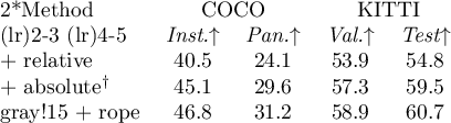
Rope encoding performs best: Recall that FFN injects temporal information about an incoming frame by conditioning the backbone \(f\) with time (Fig 3). Table
¿tbl:tab:ablation95pe? shows that the the rope-based time encoding outperforms both relative and absolute time encodings. Intuitively, rope can rotate both query/key matrices in latent space, and encode both relative/absolute positions
simultaneously.
Temporal conditioning of the backbone \(f\) helps: We perform an ablation where we remove \(t\) as a condition of the backbone \(f\) and
find that performance drops from 45.1 to \(42.7\) on COCO-Videos instance segmentation. This shows that instilling a notion of time in \(f\) helps.
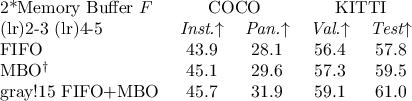
Memory buffer B can take inspiration from both FIFO/MBC policies: In Table [tbl:tab:ablation95memory95buffer], we
implement two variations of the memory buffer \(B\). MBC means that an incoming frame is merged with the ‘most-similar’ frame. MBC performs better than the FIFO queue[37]. Alternatively, one may also ‘merge’ an incoming frame (MBC) and consider it as ‘most recent’ element in a FIFO-queue6, achieving even better results.
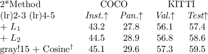
Cosine loss performs best on \(v_{latent}\): In Tab[tbl:tab:latent95loss], we experiment with different
types of loss to compute \(v_{latent}\) (in eq@eq:eq:f95latent ), and find that cosine works the best. Intuitively, cosine projects all features to a unit-hypersphere, cancels out their magnitudes, and only measures angle
difference, leading to a better estimate.
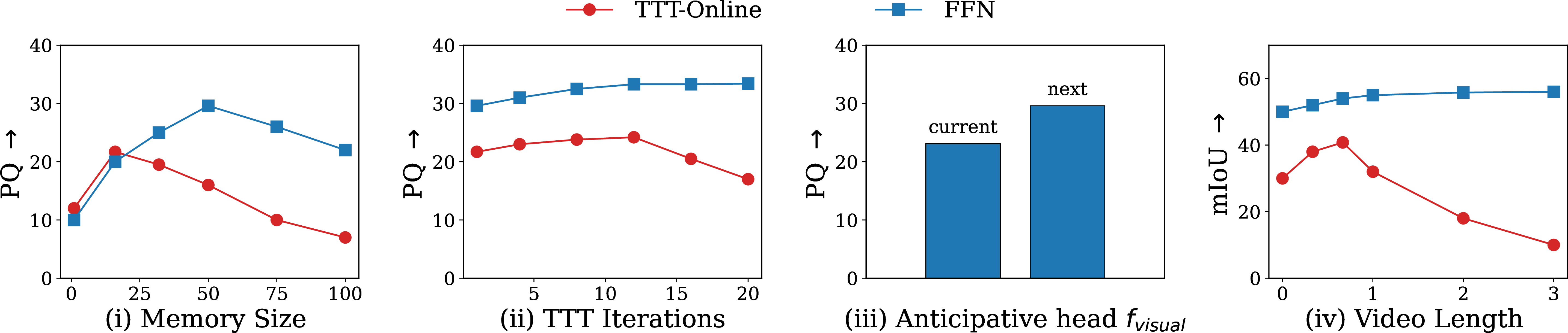
Increasing buffer length helps, but only up to a limit: In Fig5 (i), we see that FFN performs well as buffer-size increases up to \(50\) frames, then drops. This
helps validate the insight that keeping only some past-frames is important, and keeping everything worsens the performance. Intuitively, the capacity of the model \(f\) is finite, trying to
remember everything leads to instability during learning.
Increasing TTT iterations improves performance: Fig5 (ii) shows that increasing TTT iterations improves performance. Note that FFN remains almost constant, which means that it manages to learn a
lot even with just one gradient-step, whereas TTT-online needs several steps to reach its peak.
Anticipating the ‘next’ frame is better than ‘current’ frame prediction in \(f_{visual}\): Fig5 (iii) shows that it is better to predict what shall come one step in the
future, rather than just predicting the current frame, thereby showing that ‘anticipation’ can provide a unique inductive bias to a neural net.
FFN retains stable performance for long videos: In Fig5 (iv), we plot FFN’s average performance as it continues to perform TTT over 3 hour long videos on our EpicTour dataset. Note that TTT-online degrades
beyond 50 mins, whereas FFN improves/retains performance over time, indicating drift is less of an issue as compared to TTT-online. We refer the reader to supplementary material for additional ablations.
5 Related Work↩︎
There are several works operating within the regime of ‘online model distillation’ [3]: here the teacher is generally kept on the
Internet, while a student sitting on an edge-device makes decision when to adapt or not. In FFN, we aim to adapt a single model on-device and don’t require a teacher. Moreover, we focus on improving the quality of generated predictions
and not explicitly matching the real-time performance of detectors, which remains an open challenge[4].
The idea of ‘principle of locality’ can be traced back to Vapnik et al [38], [39]. This also found applications in [40], [40]–[42]. FFN’s difference lies in how it implements this locality: methods like TTT-Online[4] ‘reset’ weights after certain set of frames is processed. However, FFN’s rely on the ‘forgetting’ principle: restore a model’s baseline prior to adaptation. Although
both aim to achieve identical goals (locality), the FFN’s mechanism is different. While ideas on forgetting are typically used to unlearn ‘bad’ representations in safety-alignment[43], we showcase the application of this principle for representational-restoration.
Similarly, the computer vision community has used the idea of test-time-training for several applications [44]–[47], especially depth estimation [48]–[52]. Other works such as [53]–[56] explore online-learning and their extensions to videos [57]. Although the videos considered in such papers are mostly synthetic/very short, we also show results on long-realistic videos.
Finally, video compression algorithms [58] also implement a mechanism to measure surprise: they measure how much change a new frame
offers relative to a previous frame, which in turn is used to inform compression. The key idea is that most redundant frames are assigned short length codes[59]. However, this process is typically not learned, whereas FFN learns via an anticipative-head. Furthermore, in video-compression, the size of the file grows with the number of frames
encountered, whereas in FFN all the knowledge of a video is squeezed into a finite set of weights[60].
6 Additional Discussions↩︎
We shall now discuss some directions that might help inspire further research on FFN. Please note that while these are relevant to FFN, their precise implementation remains beyond the scope of this work. Although TTT requires only one
gradient step, it remains slow in practice. One reason is that it still relies on backpropagation. It creates a subtle ‘layer-lock’[61]: the first layer has to ‘wait’ for the gradients from the last layer to come back, thereby wasting compute cycles. Alternatives include local-learning algorithms like forward-forward[60], target propagation[62] or no-prop
[63], which can update these weights during the feed-forward phase only. A key challenge remains that these algorithms still do not surpass
backpropagation’s performance on large scale datasets.
TTT relies on the assumption that the ‘useful’ video frames keep ‘streaming’ continuously. However, there might be cases where there are no changes in the incoming frames (e.g., stationary cameras). During that time, learning does not happen, and
FFN remains idle. An alternate mechanism was discussed by [64], [65]: make FFN enter a "sleeping" phase, sample the data from within FFN itself, and perform a few iterations of gradient descent. A key challenge remains how to "sample" efficiently[66], which was later partially resolved by score-matching networks relying on Langevin dynamics[67]. Further, we showed that anticipating the next-frame works better than the current-frame prediction. This lends itself to the question: Is it
possible to meta-learn the SSL task itself. Recent works like TTT-MLP have just started exploring this interesting direction[68].
7 Conclusion↩︎
In this work, we introduced the Frame Forgetting Network (FFN): for performing test-time-training on videos which may be hours long. That is, a memory restoration mechanism allows the FFN to restore the representation of a model before adaptation. Our
key contribution is the logic of handling sliding temporal-windows by operating selectively on exiting and entering frames, rather than doing duplicate processing at each time-step.
Next, we discuss an adaptive anticipative head that decides when to do TTT on an incoming frame. Finally, we introduced the EpicTours dataset, which contains hours long videos to effectively study this important problem. Our empirical results and
ablations may help validate further merits of such an approach. In the future, we hope to explore FFN for hours long video generation [69]. May the
force be with you. May you live long and prosper.
Table of Contents
A Broader Impact
B Reproducibility Statement
C Additional Ablations
D Details of Datasets
E A brief overview of architectures
F Qualitative Demonstrations of EpicTours Dataset -
8 Broader Impact↩︎
This research introduces the Frame Forgetting Network (FFN) for efficient test-time training on long videos, along with the EpicTours dataset for benchmarking adaptation on multi-hour video streams. FFN demonstrates that test-time training can be made
computationally tractable for hours-long videos by operating on only three frames per sliding window transition. This may benefit the real-world deployment of video understanding systems in resource-constrained environments, such as edge devices,
drones, and mobile platforms.
Similarly, by removing the dependency on a remote teacher model, FFN supports fully on-device adaptation. This is particularly relevant for offline scenarios such as disaster-relief efforts, autonomous navigation, and remote surveillance, where
server connectivity may be limited or unavailable. Our adaptive windowing algorithm (AWA) reduces unnecessary computation by dynamically deciding when adaptation is needed, rather than performing TTT on every frame. This may help
contribute to more energy-efficient video processing pipelines.
We do not anticipate direct negative social impacts from this work, beyond what existing on-device models already face. However, we acknowledge that video understanding technologies, including those built on TTT, could potentially be applied in
surveillance contexts. We encourage the responsible use of such technologies, in accordance with applicable regulations and ethical guidelines.
9 Reproducibility Statement↩︎
To ensure the reproducibility of our experiments, we provide a comprehensive overview of the model architectures, hyperparameters, evaluation procedures, datasets, and baselines employed in this supplementary material. We provide complete dataset
details in 11 and architecture details in 12. Our code and data will be made publicly available for future research purposes. The videos will be made available under
the Creative Commons (CC) license.
For segmentation experiments (Tab. 1, Tab. 5), we initialize the backbone \(f\) with Mask2Former [70] pre-trained weights, train the SSL head \(g\) from scratch jointly during the training-time phase, and use Mask2Former’s pre-trained weights for the downstream head \(h\). For depth estimation (Tab. 3), we leverage the Video Depth Anything architecture [36]. For video classification
(Tab. 4), we adopt the DINOv3 [28] backbone.
Across all experiments, we set the memory buffer size \(W = 50\), perform a single gradient step per incoming frame, and use the Adam optimizer. The SSL head \(g\) is trained with
the next-frame anticipation objective instead of the current-frame reconstruction (as discussed in the main paper and validated in Fig. 5(iii)). We perform all experiments with 3 random seeds and report their mean accuracy. All experiments are
conducted on a single NVIDIA Ampere (80GB) GPU.
During the training-time phase, \(g\) may be trained on both image datasets and a single long video; the anticipative head itself can be learned with as few as one long video. At test time, the downstream
head \(h\) is kept frozen throughout, and only the backbone \(f\) and SSL head \(g\) receive gradient updates. The adaptive windowing
algorithm (AWA) uses the surprise metric \(S_t\) and the dynamic threshold \(\tau_t = \mu_t + \sigma_t\) (Eq. 7 of the main paper) to dynamically determine whether TTT is performed
on a given frame.
10 Additional Ablations↩︎
Here, we provide some additional ablations for our FFN.
| Layers | 1 | 3 | 5 | 10 |
|---|---|---|---|---|
| 41.2 | 45.1 | 43.8 | 39.5 |
10pt
Varying the number of MLP layers in the temporal module: Tab [tbl:tab:varying95mlp95layers] reveals that optimal number of layers for temporal module is \(3\).
Positional encodings do not repeat even if sampled for very long videos: Another criticism may be that FFN relies on temporally binding (a.k.a conditioning) the backbone with different timesteps. Since the positional encodings are circular, eventually they might end up repeating, which would mean that the network could no longer distinguish between timsesteps of different indices. We refer to this problem as the ‘temporal symmetry problem’.
Listing lst:positional_hash: Our Implementation of checking collisions in positional encodings.
import numpy as np
import hashlib
import collections

def get_1d_positional_encoding_np(t, d, lambda_=10000):
    """Computes sinusoidal positional encoding for a time step."""
    half_d = int(np.ceil(d / 2))
    indices = np.arange(half_d)
    inv_freq = 1.0 / (lambda_ ** (indices / (d / 2)))
    sin_inp = t * inv_freq
    emb = np.concatenate([np.sin(sin_inp), np.cos(sin_inp)])
    return emb[:d].astype(np.float32)

def get_full_float_hash(vec):
    """Computes a unique 64-bit signature from raw float memory."""
    raw_bytes = np.ascontiguousarray(vec).tobytes()
    h = hashlib.blake2b(raw_bytes, digest_size=8)
    return int(h.hexdigest(), 16)

# Configuration for temporal windows
total_time = [60, 3600, 86400, 2592000]
wavelengths = [500, 5000, 10000, 20000, 50000]
all_hashes = []

for w in wavelengths:
    for time in total_time:
        signature_hash = collections.defaultdict(int)
        for t in range(time):
            pos = get_1d_positional_encoding_np(t=t, d=2, lambda_=w)
            h = get_full_float_hash(np.sort(pos))
            signature_hash[h] += 1
        all_hashes.append({'wavelength': w, 'time': time, 'hash': signature_hash})
In the code above, we implement 1D absolute positional encodings. For a particular timestep, we return a \(d\) dimensional vector, and subsequently hash it to an integer. Simultaneously, we track potential collisions in
the hash in case two different timesteps led to the same encodings.
Key observation: We observe that this formulation does not suffer from any collisons, thereby indicating that the neural network is always given unique inputs for different time indices. We also test extreme case by
reducing the dimensionality \(d\) of positional encoding to \(2\) (one sin, another cosine) and found that it still broke symmetry. This means that the cyclic nature of sines, and cosines,
can still work. This might also help validate the idea that a particular signal can be written as a superposition of sines and cosines (fourier’s expansion)
11 Datasets↩︎
Next, we describe the details of every dataset used in our experiments.
COCO-Videos COCO-Videos [4] is a video dataset derived from the COCO benchmark, designed to evaluate test-time training in video
streams. It contains approximately 30k frames with videos averaging around 309 seconds in length. The dataset provides dense annotations suitable for evaluating both instance segmentation and panoptic segmentation.
KITTI-STEP: KITTI-STEP [14] extends the KITTI benchmark with dense, temporally consistent panoptic segmentation
annotations. It contains approximately 8k frames with video sequences averaging 40 seconds in length. The dataset includes both a validation and a test split. We report on semantic segmentation performance in terms of mIoU in both splits. KITTI-STEP is
particularly relevant to our evaluation because its driving sequences exhibit gradual scene transitions; this allows us to study how FFN’s principle of locality and adaptive windowing handle slowly evolving visual content, as opposed to the more
abrupt scene changes found in other benchmarks.
UCF101: UCF101 [71] is a widely-used action recognition benchmark containing 13,320 video clips spanning 101 action
categories. The videos are collected from YouTube and cover a diverse range of human actions. We report top-1 classification accuracy on this dataset. While our primary focus is on dense per-pixel tasks like segmentation, UCF101 allows us to evaluate
whether FFN’s adaptation mechanism can also benefit coarse video understanding.
Something-Something v2:(SSv2) [16] is a video understanding dataset that requires temporal reasoning about
object interactions. It contains more than 220k short video clips spanning 174 fine-grained action categories. Notably, SSv2 requires models to reason about the direction of time (, “moving something up” vs.”moving something down”), making it a
challenging benchmark for temporal understanding. We report top-1 classification accuracy. SSv2 is especially interesting for FFN because it tests whether our anticipative SSL objective, which predicts the next frame rather than reconstructing the
current one, can capture the temporal directionality that this benchmark demands.
ScanNet: ScanNet [19] is a richly-annotated dataset of 3D indoor scene reconstructions. It contains RGB-D video sequences
captured in a variety of indoor environments. We use ScanNet to evaluate the video depth estimation, reporting AbsRel and \(\delta_1\) metrics. Following prior work [36], we also report the Temporal Alignment Error (TAE) on a 170-frame variant of ScanNet. The TAE metric is particularly informative for FFN, as it measures temporal consistency of depth
predictions across frames; this directly tests whether FFN’s memory restoration mechanism and adaptive windowing can maintain coherent depth estimates over time.
Bonn: Bonn [20] is a dataset designed for 3D reconstruction in dynamic environments using RGB-D cameras. It provides
ground-truth depth annotations for indoor scenes. We use Bonn to evaluate video depth estimation and report AbsRel and \(\delta_1\) metrics. Unlike ScanNet and NYUv2, Bonn specifically targets dynamic indoor
environments where objects and people may move throughout the scene. This makes it a useful test of whether FFN’s adaptation can handle non-static visual content during depth estimation.
NYUv2: NYUv2 [21] is a widely-used indoor depth estimation benchmark containing RGB-D images captured with a Microsoft
Kinect sensor. It provides dense depth annotations for a variety of indoor scenes. We evaluate video depth estimation on NYUv2 and report AbsRel and \(\delta_1\) metrics. NYUv2 covers a broad range of room layouts and
furniture configurations, making it a robust generalization test. Together with KITTI (outdoor), ScanNet (indoor 3D), and Bonn (dynamic indoor), NYUv2 rounds out a diverse evaluation suite that allows us to assess FFN’s depth estimation across
varied environments and sensor characteristics.
Sintel: Sintel [22] is a synthetic benchmark derived from the open-source animated film
Sintel. It provides ground-truth depth and optical flow annotations. Following prior work, we evaluate a 50-frame variant and report AbsRel and \(\delta_1\) metrics for video depth estimation. The synthetic nature
of Sintel introduces a significant domain gap relative to the real-world datasets above; strong performance here may indicate that FFN’s self-supervised adaptation can bridge the gap between a model’s training domain and previously unseen visual
styles.
CityScapes: CityScapes [72] is a large-scale dataset to understand semantic urban scenes, containing video
sequences captured from a vehicle driving through various cities. It provides fine-grained pixel-level annotations for 19 semantic classes. As shown in Tab. 2 of the main paper, CityScapes videos average only 1.8 seconds with approximately 3k frames,
making it representative of the short-video regime that our EpicTours dataset aims to extend. We include CityScapes in Tab. 2 primarily to contextualize the scale gap: while existing benchmarks operate on seconds-long clips, FFN is designed for
videos that are orders of magnitude longer.
DAVIS: DAVIS [25] is a benchmark dataset for video object segmentation, containing densely annotated video sequences
averaging 3.5 seconds with approximately 3.4k frames. It is widely used to evaluate methods on short video clips and serves as a reference point in Tab. 2 to compare video lengths across datasets. Although DAVIS provides high-quality per-frame annotations,
its short clip lengths mean that temporal adaptation methods like FFN have limited opportunity to demonstrate their long-range benefits on this benchmark alone.
12 Architecture↩︎
12.1 Mask2Former↩︎
Our segmentation experiments employ Mask2Former [70] as the backbone architecture. Mask2Former is a universal
architecture for image segmentation that unifies semantic, instance, and panoptic segmentation under a single framework. It consists of three main components: (i) a pixel-level feature extraction backbone, (ii) a Transformer-based decoder with masked
attention, and (iii) a set of learnable object queries that produce per-segment predictions. The key innovation of Mask2Former is its masked cross-attention mechanism, which restricts attention to localized regions around predicted segments rather
than the full image, improving both efficiency and segmentation quality.
In our FFN framework, we use Mask2Former’s pre-trained backbone as \(f\) and its pre-trained task-specific head as \(h\). The SSL head \(g\) is trained
from scratch. During the training-time phase, \((f, g, h)\) are trained jointly. During test-time training, only \(f\) and \(g\) are
updated, while \(h\) is kept frozen.
12.2 TTT-MAE: Test-Time Training with Masked Autoencoders↩︎
Our self-supervised learning (SSL) task for test-time training is based on the Masked Autoencoder (MAE) framework [73], [74]. MAE operates by randomly masking a large proportion of input image patches and training the model to reconstruct the missing patches. This reconstruction task provides a strong
self-supervised signal that captures both local and global image structure. In the TTT-MAE setup [74], the MAE reconstruction objective
serves as the self-supervised task during both the training-time and test-time phases. Specifically, given an incoming frame \(x_t\), the SSL head \(g\) takes the backbone features
\(f(x_t)\) and produces a reconstruction \(x'_t = g \circ f(x_t)\). The reconstruction loss \(\ell_s(x'_t, x_t)\) is then used to update the backbone
\(f\) and SSL head \(g\) via backpropagation.
The key advantage of using MAE as the SSL task is that it does not require any external labels, making it well-suited for test-time training where ground-truth annotations are unavailable. In our FFN, we replace the standard current-frame reconstruction
objective with a next-frame anticipation objective, where the SSL head is trained to predict the upcoming frame rather than reconstruct the current one.



References↩︎
This is because neural fields work well with coordinate information[7]↩︎
This anticipative-head may be learned with as few as 1 long-video during the training phase of TTT. We also experimented with the k-step future-frame predictor[9], [10], but found the next timestep predictor to work quite well (similar to classical auto-regression in language models)↩︎
there are more numbers of pixels in \(v_{visual}\) than the dimensions in \(A\), so we multiply with the factor of \(\frac{2}{\sqrt{N}}\) in Eq@eq:eq:v95visual to compensate.↩︎
Statistically, the central limit theorem says that the majority Gaussian probability mass lies in one standard deviation, which informed this choice.↩︎
Buffer \(B\) should contain 60 frames initially. Each frame takes \(0.7sec\) for TTT, which incurs about 42 seconds of lag as \(B\) gets initialized.↩︎
After merging, we swap the merged position with last position in the FIFO queue (similar to the quicksort algorithm). This prevents the bottleneck of shifting all elements one by one to achieve sorting. The former operation is a single swap, whereas the latter is computationally expensive (and CPU becomes the bottleneck instead of GPU).↩︎