On the sum of the two largest eigenvalues of the curl-curl operator on graphs
June 25, 2026
Abstract
The Grone–Merris conjecture, proved by Bai in 2011, states that the spectrum of the graph Laplacian \(\Delta_0 = -\operatorname{div}\operatorname{grad}\) is majorized by the conjugate of the vertex degree sequence. Duval and Reiner proposed a simplicial complex analogue of this statement. On a graph, where triangles serve as \(2\)-simplices, their conjecture reduces to the assertion that the spectrum of \(\operatorname{curl}^*\operatorname{curl}\) is majorized by the conjugate of the second-order degree sequence, which records the number of triangles containing each vertex.
We prove that the sum of the two largest eigenvalues of \(\operatorname{curl}^*\operatorname{curl}\) does not exceed the sum of the first two entries of that conjugate sequence. This confirms the first two majorization inequalities predicted by Duval and Reiner for \(\operatorname{curl}^*\operatorname{curl}\). As a corollary, we obtain upper bounds for the two largest eigenvalues of the full graph Helmholtzian \(\Delta_1 = -\operatorname{grad}\operatorname{div} + \operatorname{curl}^*\operatorname{curl}\). The same result extends to the up-Laplacian of any \(3\)-family, yielding a concrete step towards the Duval–Reiner conjecture in dimension \(1\).
Keywords: Graph Laplacian, Curl-curl operator, Graph Helmholtzian
MSC(2020). 05C50, 05C65, 05E45.
1 Introduction↩︎
Let \(G\) be a simple graph with vertex set \(V(G)\) and edge set \(E(G)\), and let \(T(G)\) denote the set of triangles in \(G\). We consider real-valued functions \[f: V(G)\to\mathbb{R},\qquad X: V(G)\times V(G)\to\mathbb{R},\qquad \Phi: V(G)\times V(G)\times V(G)\to\mathbb{R},\] where \(X\) and \(\Phi\) are alternating on \(E(G)\) and \(T(G)\), respectively. More precisely, \[X(v_i,v_j)= \begin{cases} -X(v_j,v_i), & \text{if } \{v_i,v_j\}\in E(G),\\ 0, & \text{otherwise}, \end{cases}\] and for every \(\{v_i,v_j,v_k\}\in T(G)\), \[\Phi(v_i,v_j,v_k)=\Phi(v_j,v_k,v_i)=\Phi(v_k,v_i,v_j) =-\Phi(v_j,v_i,v_k)=-\Phi(v_i,v_k,v_j)=-\Phi(v_k,v_j,v_i),\] while \(\Phi(v_i,v_j,v_k)=0\) if \(\{v_i,v_j,v_k\}\notin T(G)\). We denote by \(L^2(V(G))\), \(L^2_{\wedge}(E(G))\) and \(L^2_{\wedge}(T(G))\) the spaces of functions of the above three types; the subscript \(\wedge\) emphasizes the alternating property.
In the language of algebraic topology, \(f\), \(X\) and \(\Phi\) are \(0\)-, \(1\)- and \(2\)-cochains, respectively. They can be viewed as discrete analogues of differential forms on a smooth manifold [1] and are often called discrete differential forms [2], [3], with \(f\), \(X\) and \(\Phi\) regarded as \(0\)-, \(1\)- and \(2\)-forms on \(G\). We equip these spaces with the standard inner products \[\left\{\begin{array}{l} \langle f,g\rangle_{L^2(V(G))} =\sum_{v\in V(G)}f(v)g(v), \\[2mm] \langle X,Y\rangle_{L^2_{\wedge}(E(G))} =\sum_{(v_i,v_j)\in E(G)}X(v_i,v_j)Y(v_i,v_j),\\[2mm] \langle \Phi,\Psi\rangle_{L^2_{\wedge}(T(G))} =\sum_{(v_i,v_j,v_k)\in T(G)}\Phi(v_i,v_j,v_k)\Psi(v_i,v_j,v_k), \end{array}\right.\] for any \(f,g\in L^2(V(G))\), \(X,Y\in L^2_{\wedge}(E(G))\) and \(\Phi,\Psi\in L^2_{\wedge}(T(G))\).
We now introduce the discrete differential operators that generalize gradient, curl and divergence from vector calculus; a detailed exposition can be found in [4]. The graph gradient \(\operatorname{grad} : L^2(V(G))\to L^2_{\wedge}(E(G))\) is defined by \[(\operatorname{grad}f)(v_i,v_j)= \begin{cases} f(v_j)-f(v_i), & \text{if } \{v_i,v_j\}\in E(G),\\ 0, & \text{otherwise}. \end{cases}\] The graph curl \(\operatorname{curl} : L^2_{\wedge}(E(G))\to L^2_{\wedge}(T(G))\) is defined by \[(\operatorname{curl}X)(v_i,v_j,v_k)= \begin{cases} X(v_i,v_j)+X(v_j,v_k)+X(v_k,v_i), & \text{if } \{v_i,v_j,v_k\}\in T(G),\\ 0, & \text{otherwise}. \end{cases}\] The graph divergence \(\operatorname{div} : L^2_{\wedge}(E(G))\to L^2(V(G))\) is given by \[(\operatorname{div}X)(v_i)=\sum_{v_j\in V(G)}X(v_i,v_j),\] where the sum is over all vertices, but the alternating property of \(X\) ensures that only neighbors contribute.
Associated with these discrete differential operators are two fundamental Hodge-type operators. The first is the graph Laplacian \(\Delta_0 : L^2(V(G))\to L^2(V(G))\), defined by \[\Delta_0 = -\operatorname{div}\operatorname{grad},\] which serves as a graph-theoretic analogue of the Laplace operator (cf.[4]). The second is the graph Helmholtzian [5], \[\Delta_1 = -\operatorname{grad}\operatorname{div} + \operatorname{curl}^*\operatorname{curl},\] which is a discrete analogue of the vector Laplacian. Here \(\operatorname{curl}^* : L^2_{\wedge}(T(G))\to L^2_{\wedge}(E(G))\) is the adjoint of \(\operatorname{curl}\) with respect to the inner products on \(L^2_{\wedge}(E(G))\) and \(L^2_{\wedge}(T(G))\). Using the adjoint relation \[\langle \operatorname{curl}X,\Phi\rangle_{L^2_{\wedge}(T(G))} = \langle X,\operatorname{curl}^*\Phi\rangle_{L^2_{\wedge}(E(G))},\] one obtains the explicit formula \[(\operatorname{curl}^*\Phi)(v_i,v_j)= \begin{cases} \displaystyle\sum_{v_k\in V(G)}\Phi(v_i,v_j,v_k), & \text{if } \{v_i,v_j\}\in E(G),\\ 0, & \text{otherwise}, \end{cases}\] for any \(\Phi\in L^2_{\wedge}(T(G))\).
For a linear operator \(\mathcal{A}\), let \(\mathbf{s}(\mathcal{A})\) denote the weakly decreasing rearrangement of its eigenvalues (counting multiplicities). The nilpotency conditions \(\operatorname{curl}\operatorname{grad}=0\) and \(\operatorname{div}\operatorname{curl}^*=0\) (see [4]) imply \[(-\operatorname{grad}\operatorname{div})\circ(\operatorname{curl}^*\operatorname{curl}) = 0 = (\operatorname{curl}^*\operatorname{curl})\circ(-\operatorname{grad}\operatorname{div}).\] Consequently, the nonzero spectrum of \(\Delta_1\) is the multiset union of the nonzero spectra of \(-\operatorname{grad}\operatorname{div}\) and \(\operatorname{curl}^*\operatorname{curl}\), \[\label{eq-01} \mathbf{s}(\Delta_1) \stackrel{\circ}{=} \mathbf{s}(-\operatorname{grad}\operatorname{div}) \uplus \mathbf{s}(\operatorname{curl}^*\operatorname{curl}),\tag{1}\] where \(\uplus\) denotes multiset union and \(\stackrel{\circ}{=}\) means equality up to zero eigenvalues. Moreover, by standard linear algebra, we get \[\label{eq-02} \mathbf{s}(-\operatorname{grad}\operatorname{div}) \stackrel{\circ}{=} \mathbf{s}(-\operatorname{div}\operatorname{grad}) = \mathbf{s}(\Delta_0),\tag{2}\] and the operators \(\operatorname{curl}^*\operatorname{curl}\), \(-\operatorname{grad}\operatorname{div}\) and \(\Delta_0\) are all self-adjoint and positive semidefinite; hence all eigenvalues involved are real and nonnegative.
Let \(\mathbf{x}=(x_1,\ldots,x_n)\) and \(\mathbf{y}=(y_1,\ldots,y_n)\) be two non-negative sequences which are ordered non-increasing. We say \(\mathbf{x}\) is majorized by \(\mathbf{y}\), denoted \(\mathbf{x}\prec \mathbf{y}\), if \(\sum_{i=1}^kx_i\le \sum_{i=1}^ky_i\) for \(1\le k\le n\) and \(\sum_{i=1}^nx_i=\sum_{i=1}^ny_i\). The conjugate sequence of \(\mathbf{x}\), denoted by \(\mathbf{x}^\top=(x_1^\top,\cdots,x_n^\top)\), is defined by \(x_i^\top=|\{j\mid x_j\ge i\}|\). In 1994, Grone and Merris [6] conjectured that the eigenvalues of the graph Laplacian \(\Delta_0\) are majorized by the conjugate of the vertex degree sequence; this was proved by Bai [7] in 2011. Duval and Reiner [8] proposed a far-reaching analogue for simplicial complexes, formulated in terms of boundary operators.
Conjecture 1 ([8]). Let \(K\) be a \(k\)-family on vertex set \(V(K)\) and let \(\mathbf{s}=(s_1\ge s_2\ge\cdots)\) be the nonincreasing sequence of nonzero eigenvalues of \(\partial_{k-1}\partial_{k-1}^*\). Let \(\mathbf{d}=(d_1\ge d_2\ge\cdots)\) be the vertex degree sequence of \(K\). Then \(\mathbf{s}\prec \mathbf{d}^\top\), where \(\prec\) denotes majorization.
For a graph \(G\), the edge set \(E(G)\) is exactly a \(2\)-family. Therefore, \(\partial_{1}\partial_{1}^{*}\) coincides with the graph Laplacian \(\Delta_0 = -\operatorname{div}\operatorname{grad}\), thereby recovering the Grone–Merris conjecture. Also, the triangle set \(T(G)\) is a \(3\)-families, and the operator \(\partial_{2}\partial_{2}^{*}\) for such family coincides with \(\operatorname{curl}^{*}\operatorname{curl}\). Thus, to make progress on Conjecture 1 beyond the case \(k=2\), we focus on the operator \(\operatorname{curl}^*\operatorname{curl}\) and, more generally, on the graph Helmholtzian \(\Delta_1\). We establish a sharp upper bound for the sum of the two largest eigenvalues of \(\operatorname{curl}^*\operatorname{curl}\), and then transfer this bound to \(\Delta_1\).
For a vertex \(v\in V(G)\), let \(\deg_G(v)\) be the standard degree (number of incident edges) and \(\deg_G^{(2)}(v)\) be the second-order degree, i.e., the number of triangles containing \(v\). Denote the conjugate sequences of the vertex degree sequence and the second-order degree sequence by \(d^\top(G)\) and \(D^\top(G)\), respectively. Explicitly, for \(i\ge 1\), \[d_i^\top(G) = \bigl|\{v\in V(G): \deg_G(v)\ge i\}\bigr|,\qquad D_i^\top(G) = \bigl|\{v\in V(G): \deg_G^{(2)}(v)\ge i\}\bigr|.\]
Our first main result is the following majorization-type inequality for \(\operatorname{curl}^*\operatorname{curl}\).
Theorem 1. For any graph \(G\), we have \[\label{eq-m-1} \lambda_1\left(\operatorname{curl}^*(G)\operatorname{curl}(G)\right) + \lambda_2(\operatorname{curl}^*(G)\operatorname{curl}(G)) \le D_1^\top(G) + D_2^\top(G),\qquad{(1)}\] where \(\lambda_i\left(\operatorname{curl}^*(G)\operatorname{curl}(G)\right)\) denotes the \(i\)-th largest eigenvalue of \(\operatorname{curl}^*\operatorname{curl}\).
Combining 1 and 2 , we have \[\label{eq-l-a-1} \mathbf{s}(\Delta_1) \stackrel{\circ}{=} \mathbf{s}(\Delta_0) \uplus \mathbf{s}(\operatorname{curl}^*\operatorname{curl}).\tag{3}\] Moreover, \[d_1^\top(G)\ge d_2^\top(G)\ge D_1^\top(G) \ge D_2^\top(G).\] This spectral decomposition, together with the above inequalities, allows us to control the top eigenvalues of the Helmholtzian.
Corollary 1. Let \(G\) be a graph. Then the sum of the two largest eigenvalues of \(\Delta_1\) satisfies the following bounds.
If both \(\lambda_1(\Delta_1)\) and \(\lambda_2(\Delta_1)\) belong to \(\mathbf{s}(\operatorname{curl}^*\operatorname{curl})\), then \[\lambda_1(\Delta_1)+\lambda_2(\Delta_1) \le D_1^\top(G)+D_2^\top(G).\]
If neither \(\lambda_1(\Delta_1)\) nor \(\lambda_2(\Delta_1)\) belongs to \(\mathbf{s}(\operatorname{curl}^*\operatorname{curl})\), then \[\lambda_1(\Delta_1)+\lambda_2(\Delta_1) \le d_1^\top(G)+d_2^\top(G).\]
Otherwise, \(\lambda_1(\Delta_1)+\lambda_2(\Delta_1) \le d_1^\top(G)+D_1^\top(G).\)
The above estimates are obtained for graphs, but the result for \(\operatorname{curl}^*\operatorname{curl}\) yields a corresponding bound for the up-Laplacian of a general \(3\)-family, which need not be realizable as the family of triangles of a graph. Let \(K\) be a \(3\)-family on vertex set \(V(K)\). For any \(i\in V(K)\), its degree \(\operatorname{deg}_K(i)\) is the number of \(3\)-sets in \(K\) that contain \(i\). Let \(\mathbf{d}(K)=(d_1(K)\ge d_2(K)\ge\cdots)\) be the vertex degree sequence of \(K\), and let \(\mathbf{d}^{\top}(K)=(d_1^\top(K)\ge d_2^\top(K)\ge\cdots)\) denote its conjugate degree sequence.
Corollary 2. Let \(K\) be a \(3\)-family on vertex set \(V(K)\). Then \[\lambda_1(\partial_{2}(K)\partial_{2}^*(K)) + \lambda_2(\partial_{2}(K)\partial_{2}^*(K)) \le d_1^\top(K) + d_2^\top(K),\] where \(\partial_{2}(K)\partial_{2}^*(K)\) denotes the up-Laplacian of \(K\).
2 Preliminaries↩︎
We begin by recalling a classical result on eigenvalues of symmetric matrices that will be used repeatedly.
Lemma 1 (Ky Fan’s inequality [9]). Let \(A,B\in\mathbb{R}^{n\times n}\) be symmetric matrices, and let \(1\le k\le n\). Then \[\sum_{i=1}^k \lambda_i(A+B) \le \sum_{i=1}^k \lambda_i(A) + \sum_{i=1}^k \lambda_i(B).\]
2.1 Oriented incidence structure and matrix representations↩︎
We now give the matrix representations of the operators \(-\operatorname{grad}\operatorname{div}\), \(\operatorname{curl}^{*}\operatorname{curl}\), and \(\Delta_1\). Let \(G\) be a simple graph with vertex set \(V(G)\), edge set \(E(G)\), and triangle set \(T(G)\). We fix arbitrary orientations on all edges and on all triangles.
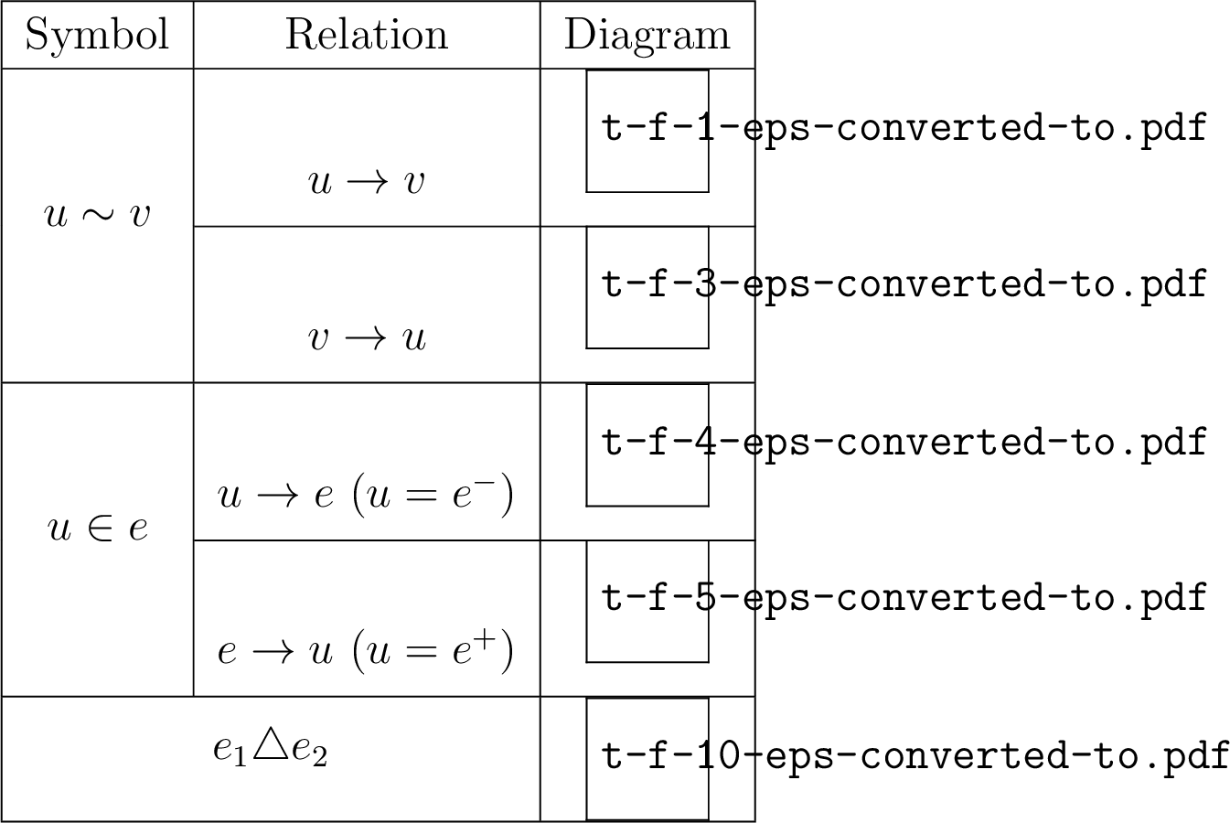
For an oriented edge \(e\), we denote its tail and head by \(e^{-}\) and \(e^{+}\), respectively, and write \(V(e)=\{e^{-},e^{+}\}\). If there is an oriented edge from \(u\) to \(v\), we write \(u\to v\). If \(u\) and \(v\) are adjacent, we write \(u\sim v\); otherwise \(u\nsim v\). For a vertex \(v\) and an edge \(e\), we write \(v\in e\) if \(v\in V(e)\), and we write \(v\to e\) if \(v=e^{-}\), \(e\to v\) if \(v=e^{+}\).
For two edges \(e_1,e_2\in E(G)\), we write \(e_1\sim e_2\) if \(V(e_1)\cap V(e_2)\neq\varnothing\). Furthermore:
\(e_1\to e_2\) if \(e_1^{+}=e_2^{-}\);
\(e_1\stackrel{+}{\sim}e_2\) if \(e_1^{+}=e_2^{+}\), and \(e_1\stackrel{-}{\sim}e_2\) if \(e_1^{-}=e_2^{-}\);
\(e_1\stackrel{\pm}{\sim}e_2\) if either \(e_1\stackrel{+}{\sim}e_2\) or \(e_1\stackrel{-}{\sim}e_2\);
\(e_1\leftrightarrow e_2\) if either \(e_1\to e_2\) or \(e_2\to e_1\);
\(e_1\triangle e_2\) if \(e_1\) and \(e_2\) belong to a common triangle.
For an edge \(e\) and a triangle \(\triangle\), we write \(e\in\triangle\) if \(e\) is an edge of \(\triangle\). If the orientation of \(e\) is compatible with that of \(\triangle\), we write \(e\in\triangle^{+}\); otherwise \(e\in\triangle^{-}\). The triangle degree of an edge \(e\in E(G)\) is defined by \(\deg_G(e) = \bigl|\{\triangle\in T(G) \mid e\in\triangle\}\bigr|\).
For clarity, we summarize the above conventions in Table ¿tbl:tab-a-1?.

The edge–vertex incidence matrix of \(G\), denoted by \(\mathcal{B}=(\mathcal{B}_{ev})\), is the matrix with rows indexed by \(E(G)\) and columns by \(V(G)\). The triangle–edge incidence matrix, denoted by \(\mathcal{C}=(\mathcal{C}_{\triangle e})\), is the matrix with rows indexed by \(T(G)\) and columns by \(E(G)\). They are defined by \[\mathcal{B}_{ev}= \begin{cases} -1, & \text{if } v\to e,\\ 1, & \text{if } e\to v,\\ 0, & \text{otherwise}, \end{cases} ~\text{and}~ \mathcal{C}_{\triangle e}= \begin{cases} -1, & \text{if } e\in\triangle^{-},\\ 1, & \text{if } e\in\triangle^{+},\\ 0, & \text{otherwise}. \end{cases}\]
According to [4], the matrix representations of \(-\operatorname{grad}\operatorname{div}\) and \(\operatorname{curl}^{*}\operatorname{curl}\) are given by \(\mathcal{B}\mathcal{B}^\top\) and \(\mathcal{C}^\top\mathcal{C}\), respectively. Their entries are described explicitly below.
Lemma 2 ([4]). Let \(G\) be a graph with fixed orientations on \(E(G)\) and \(T(G)\). Then the matrix representing \(-\operatorname{grad}\operatorname{div}\) is \(\mathcal{B}\mathcal{B}^\top\), indexed by \(E(G)\), with entries \[(\mathcal{B}\mathcal{B}^\top)_{ee'}= \begin{cases} 2, & \text{if } e' = e,\\[2pt] -1, & \text{if } e \leftrightarrow e',\\[2pt] 1, & \text{if } e' \overset{\pm}{\sim} e,\\[2pt] 0, & \text{otherwise}. \end{cases}\]
Lemma 3 ([4]). Under the same assumptions, the matrix representing \(\operatorname{curl}^{*}\operatorname{curl}\) is \(\mathcal{C}^\top\mathcal{C}\), indexed by \(E(G)\), with entries \[(\mathcal{C}^\top\mathcal{C})_{ee'}= \begin{cases} \deg_G(e), & \text{if } e' = e,\\[2pt] 1, & \text{if } e \leftrightarrow e' \text{ and } e \triangle e',\\[2pt] -1, & \text{if } e' \overset{\pm}{\sim} e \text{ and } e \triangle e',\\[2pt] 0, & \text{otherwise}. \end{cases}\]
Lemma 4. The spectrum of \(\operatorname{curl}^{*}\operatorname{curl}\) is independent of the choice of orientations on \(E(G)\) and \(T(G)\).
Proof. Let \(\gamma_1\) and \(\gamma_2\) be two distinct choices of orientations on \(E(G)\) and \(T(G)\), and let \(\mathcal{C}\) and \(\mathcal{C}^{\prime}\) denote the corresponding triangle–edge incidence matrices associated with these orientations, respectively. Let \(E\) be a diagonal sign matrix indexed by \(E(G)\), defined by \[E_{ee} = \begin{cases} 1, & \text{if the orientation of } e \text{ is the same under } \gamma_1 \text{ and } \gamma_2,\\ -1, & \text{otherwise}. \end{cases}\] As shown in Lemma 3, the entrywise structure of the incidence relation between edges and triangles is invariant under simultaneous preservation or reversal of the orientations of \(e\) and \(e'\). In all other cases, the only effect of changing orientations is an interchange of signs in the cases \(e \leftrightarrow e'\) and \(e' \overset{\pm}{\sim} e\), while all other relations remain unchanged. Consequently, by Lemma 3, we obtain \[\left(\mathcal{C}^{\prime\top}\mathcal{C}^\prime\right)_{ee'} = E_{e,e}\left(\mathcal{C}^{\top}\mathcal{C}\right)_{ee'}E_{e^{\prime}e^{\prime}},\] and hence \(\mathcal{C}^{\prime\top}\mathcal{C}^\prime= E^{\top}\left(\mathcal{C}^{\top}\mathcal{C} \right)E.\) Since \(E\) is a diagonal matrix with entries \(\pm 1\), we have \(E^{-1}=E^{\top}=E\). Therefore, \[\mathcal{C}'^{\top}\mathcal{C}' = E^{-1}(\mathcal{C}^{\top}\mathcal{C})E,\] so \(\mathcal{C}'^{\top}\mathcal{C}'\) and \(\mathcal{C}^{\top}\mathcal{C}\) are similar matrices. Consequently, they have the same spectrum, which completes the proof. ◻
Since \(\Delta_1 = -\operatorname{grad}\operatorname{div} + \operatorname{curl}^{*}\operatorname{curl}\), its matrix representation follows immediately.
Lemma 5. Let \(G\) be a graph with orientations on \(E(G)\) and \(T(G)\). Then the graph Helmholtzian is represented by the matrix \(\mathcal{H}(G)=(h_{ee'})=\mathcal{B}\mathcal{B}^{\top}+\mathcal{C}^{\top}\mathcal{C}\), indexed by \(E(G)\), where \[h_{ee'}= \begin{cases} \deg_G(e)+2, & \text{if } e' = e,\\[2pt] -1, & \text{if } e \leftrightarrow e' \text{ and } e \mathrel{\ooalign{\triangle\cr\hidewidth/\hidewidth\cr}}e',\\[2pt] 1, & \text{if } e' \overset{\pm}{\sim} e \text{ and } e \mathrel{\ooalign{\triangle\cr\hidewidth/\hidewidth\cr}}e',\\[2pt] 0, & \text{otherwise}. \end{cases}\]
2.2 Known bounds for the largest eigenvalue↩︎
We also record three known estimates for the largest eigenvalue of \(\operatorname{curl}^{*}\operatorname{curl}\) that follow from earlier work on simplicial complexes.
Lemma 6 ([8]). Let \(G\) be a graph with vertex set \(V(G)\), edge set \(E(G)\), and triangle set \(T(G)\). Then \[\lambda_1(\operatorname{curl}^{*}(G)\operatorname{curl}(G)) \le D_1^\top(G).\]
Lemma 7 ([8]). Let \(G\) be a graph with vertex set \(V(G)\), edge set \(E(G)\), and triangle set \(T(G)\). Then \[\lambda_1(\operatorname{curl}^{*}(G)\operatorname{curl}(G)) \ge \max\{\deg_G(e) \mid e\in E(G)\} + 2.\]
Lemma 8 ([10]). Let \(G\) be a graph with vertex set \(V(G)\), edge set \(E(G)\), and triangle set \(T(G)\). Then \[\lambda_1(\operatorname{curl}^{*}(G)\operatorname{curl}(G)) \le \max\Bigl\{\,\sum_{e\in\triangle}\deg_G(e) \mid \triangle\in T(G)\Bigr\}.\]
3 Proofs of the main results↩︎
Before proceeding with the proof, we fix some notation and standing assumptions that will be used throughout this section. For two vertex disjoint graphs \(G_1\) and \(G_2\), denote by \(G_1\cup G_2\) the union of them. That is, \(V(G_1\cup G_2)=V(G_1)\cup V(G_2)\) and \(E(G_1\cup G_2)=E(G_1)\cup E(G_2)\). Their join \(G_1\vee G_2\) is the graph obtained from \(G_1\cup G_2\) by adding all possible edges between \(G_1\) and \(G_2\). The union of \(t\) copies of a graph \(H\) is denoted by \(tH\). As usual, we use \(K_n\), \(P_n\), and \(C_n\) to denote the complete graph, the path, and the cycle on \(n\) vertices, respectively.
Let \(G\) be a graph with vertex set \(V(G)\), edge set \(E(G)\), and triangle set \(T(G)\). Recall that, for a vertex \(v\in V(G)\), its second-order degree is defined as \(\deg_G^{2}(v)=|\{\triangle\mid v\in \triangle\}|\). Let \(V_1(G) = \{v \in V(G) \mid \deg_G^{(2)}(v) = 1\}\) and \(V_2(G) = \{v \in V(G)\mid \deg_G^{(2)}(v) \ge 2\}\). For a positive integer \(i\), denote by \(D_i^{\top}(G)=\{v\in V(G)\mid \deg_G^{(2)}(v)\ge i\}\). Also, for an edge \(e\in E(G)\), denote by \(\deg_G(e)\) the number of triangles containing \(e\). For positive integers \(n,k,a_1,\ldots,a_k\), denote by \(\mathcal{G}_{n;k}^{a_1,\ldots,a_k}\) the set of graphs obtained from \(K_n\) by choosing \(k\) distinct edges, and then, for each \(1\le i\le k\), attaching \(a_i\) pairwise nonadjacent new vertices, each of which is joined to both endpoints of the \(i\)-th chosen edge.
3.1 Proof of Theorem 1↩︎
Note that if \(\deg_G^{(2)}(v)=0\) for some vertex \(v\in V(G)\), then every edge incident with \(v\) does not belong to any triangle. Consequently, the corresponding rows and columns in the matrix representation \(\mathcal{C}^\top(G)\mathcal{C}(G)\) are zero, and hence such edges contribute only to the multiplicity of the eigenvalue \(0\). Therefore, without loss of generality, we restrict our attention to graphs in which every edge (as well as every vertex) is contained in at least one triangle. Therefore, for a graph \(G\), we may assume that \(D_1^\top(G)=|V(G)|\), \(V(G)=V_1(G)\sqcup V_2(G)\), and \(D_2^\top(G) = |V_2(G)|\). In what follows, we show that Eq. ?? always holds.
According to Lemma 6, we have \[\label{eq-dr-1} \lambda_1\left(\operatorname{curl}^*(G)\operatorname{curl}(G)\right)\le D_1^{\top}(G)\tag{4}\] If \(\lambda_2(\operatorname{curl}^*(G)\operatorname{curl}(G))=0\), then we obtain \[\lambda_1\left(\operatorname{curl}^*(G)\operatorname{curl}(G)\right) +\lambda_2\left(\operatorname{curl}^*(G)\operatorname{curl}(G)\right) \le D_1^{\top}(G),\] and ?? follows immediately. Therefore, without loss of generality, we may assume that \(\operatorname{curl}^*(G)\operatorname{curl}(G)\) has at least two nonzero eigenvalues. This in turn leads to \(t(G)\ge 2\).
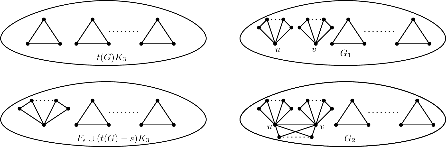
First, we consider the case for \(D_2^{\top}(G)\le 2\). If \(D_2^{\top}(G)=0\), then \(G\cong t(G)K_3\). If \(D_2^{\top}(G)=1\), then \(G\cong F_s\cup (t(G)-s)K_3\) for some \(s\ge 2\), where \(F_s=K_1\vee (sK_2)\) is the friendship graph. If \(D_2^{\top}(G)=2\), then assume \(V_2(G)=\{u,v\}\). Therefore, we conclude that either \(G\cong G_1\) when \(u\not\sim v\), or \(G\cong G_2\) when \(u\sim v\) (shown in Fig. 1). One can verify such cases by directed calculations. We omit the calculations here but put them in Appendix 4.
Next, we consider the case for \(D_2^{\top}(G)\ge 3\). We divide the following two cases to discuss.
Case 1. There exists a triangle \(\triangle \in T(G)\) such that \(\left|\triangle\cap V_1(G)\right|\ge 2\).
We proceed by induction on \(t(G)\). Since \(D_2^{\top}(G)\ge 3\), we have \(t(G)\ge 3\). If \(t(G)=3\), then \(G\cong G_4\) (see Figure 2).
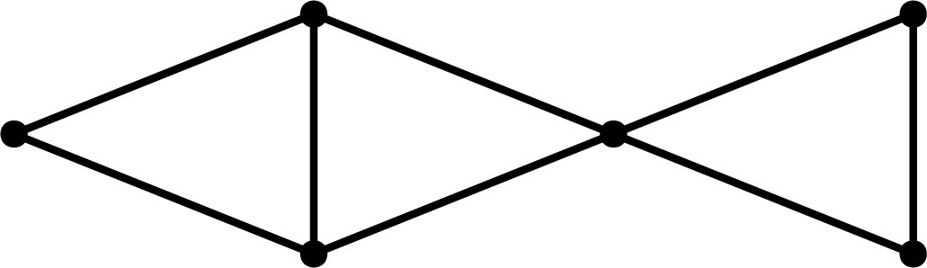
Then \(\mathbf{s}\left(\operatorname{curl}^*(G)\operatorname{curl}(G)\right)\stackrel{\circ}{=}\left\{4,3,2\right\}\), and thus we have \(\lambda_2\left(\operatorname{curl}^*(G)\operatorname{curl}(G)\right)=3\le D_2^{\top}(G)\), and ?? follows. Suppose now that the induction hypothesis holds for all graphs with fewer than \(t(G)\) triangles. Choose a triangle \(\triangle\in T(G)\) such that \(\left|\triangle\cap V_1(G)\right|\ge 2\). Let \(e\) be an edge of \(\triangle\) with both endpoints in \(V_1(G)\), and let \(G_0=G-e\). Then \(\triangle\) shares no edge with any other triangle. Therefore, one can easily verify that \[\mathbf{s}(\operatorname{curl}^*(G)~\operatorname{curl}(G))=\mathbf{s}(\operatorname{curl}^*(G_0)~\operatorname{curl}(G_0))\uplus \{3\}.\] If \(\lambda_2(\operatorname{curl}^*(G)~\operatorname{curl}(G))\le 3\), then ?? holds immediately due to 4 and the assumption \(D_2^{\top}(G)\ge 3\). If \(\lambda_2(\operatorname{curl}^*(G)~\operatorname{curl}(G))\ge 4\), then \[\label{eq-thm-2} \lambda_i\!\left(\operatorname{curl}^*(G_0)\operatorname{curl}(G_0)\right)=\lambda_i\!\left(\operatorname{curl}^*(G)\operatorname{curl}(G)\right)\quad\text{for} \quad i\in\{1,2\}.\tag{5}\] Moreover, if \(|\triangle\cap V_1(G)|=3\), then \(D_1^{\top}(G_0)=D_1^{\top}(G)-3\) and \(D_2^{\top}(G_0)=D_2^{\top}(G)\); if \(|\triangle\cap V_1(G)|=2\), then either \(D_1^\top\left(G_0\right)=D_1^\top\left(G\right)-2\) and \(D_2^\top\left(G_0\right)=D_2^\top\left(G\right)\), or \(D_1^\top\left(G_0\right)=D_1^\top\left(G\right)-1\) and \(D_2^\top\left(G_0\right)=D_2^\top\left(G\right)-1.\) In all cases, we always have \[\label{eq-a-1} D_1^{\top}(G_0)+D_2^{\top}(G_0)\le D_1^{\top}(G)+D_2^{\top}(G)-2.\tag{6}\] By the inductive assumption, combining 5 and 6 , we get \[\begin{array}{ll} &\lambda_1(\operatorname{curl}^*(G)\operatorname{curl}(G))+\lambda_2(\operatorname{curl}^*(G)\operatorname{curl}(G))\\[2mm] =& \lambda_1(\operatorname{curl}^*(G_0)\operatorname{curl}(G_0))+\lambda_2(\operatorname{curl}^*(G_0)\operatorname{curl}(G_0))\\[2mm] \le&D_1^{\top}(G_0)+D_2^{\top}(G_0)\le D_1^{\top}(G)+D_2^{\top}(G)-2, \end{array}\] as desired.
Case 2. \(|\triangle\cap V_1(G)|\le 1\) for every \(\triangle\in T(G)\).
If \(V_1(G)=\emptyset\), then we have \[D_1^\top(G) = |V(G)|=|V_1(G)|+|V_2(G)|=|V_2(G)|=D_2^\top(G).\] Thus, 4 indicates \[\begin{array}{ll} &\lambda_1\left(\operatorname{curl}^{*}(G)\operatorname{curl}(G)\right)+ \lambda_2\left(\operatorname{curl}^{*}(G)\operatorname{curl}(G)\right) \\[2mm] \le & 2\lambda_1\left(\operatorname{curl}^{*}(G)\operatorname{curl}(G)\right) \le 2D_1^\top(G)= D_1^\top(G)+D_2^\top(G), \end{array}\] as desired.
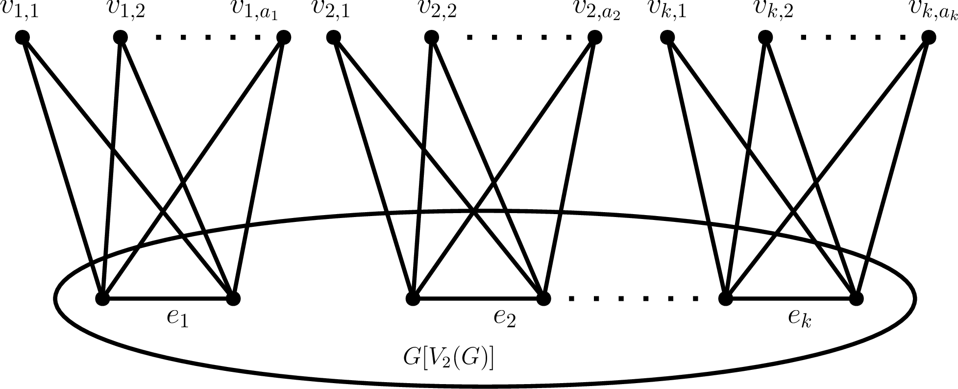
If \(V_1(G)\ne\emptyset\), then for every \(v\in V_1(G)\), there exists a unique edge \(e\) in \(G[V_2(G)]\) such that \(e\cup\{v\}\) forms a triangle, i.e., \(e\cup\{v\}\in T(G)\). For an edge \(e\in G[V_2(G)]\), denote by \[V_{1,e}=\{v\in V_1(G)\mid e\cup v\in T(G)\}.\] Assume that \(e_1,\ldots,e_k\) are all the edges in \(G[V_2(G)]\) with \(V_{1,e_i}\ne\emptyset\). Let \(a_i=|V_{1,e_i}|\) for \(1\le i\le k\). We may assume that \(a_1\ge a_2\ge\cdots\ge a_k\ge 1\). Thus, \(V_1(G)=\cup_{1\le i\le k}V_{1,e_i}\) and \(G\) has the structure as shown in Figure 3.
For convenience, denote by \(T=T(G)\), \(T_1=\{\triangle\in T(G)\mid \triangle\cap V_1(G)\ne\emptyset\}\), and \(T_2=\{\triangle\in T(G)\mid \triangle\cap V_1(G)=\emptyset\}\). Consider the \(3\)-families \(T\), \(T_1\) and \(T_2\). Then from \(T=T_1\sqcup T_2\) and the definition of \(\partial_{2}\partial_{2}^*\) (see [8]), it follows that \[\label{eq-l-00} \partial_{2}(T)\partial_{2}^*(T)=\partial_{2}(T_1)\partial_{2}^*(T_1)+\partial_{2}(T_2)\partial_{2}^*(T_2),\tag{7}\] and that the \(\partial_{2}(T)\partial_{2}^{*}(T)=\operatorname{curl}^{*}(G)\operatorname{curl}(G)\) . Therefore, combining Eq. 7 and Lemma 1, we get \[\label{eq-l-1} \begin{array}{ll} &\lambda_1\left(\operatorname{curl}^{*}(G)\operatorname{curl}(G)\right)+ \lambda_2\left(\operatorname{curl}^{*}(G)\operatorname{curl}(G)\right)\\[2mm] \le&\lambda_1\left(\partial_{2}(T_1)\partial_{2}^*(T_1)\right)+ \lambda_2\left(\partial_{2}(T_1)\partial_{2}^*(T_1)\right)+\lambda_1\left(\partial_{2}(T_2)\partial_{2}^*(T_2)\right) + \lambda_2\left(\partial_{2}(T_2)\partial_{2}^*(T_2)\right). \end{array}\tag{8}\] By noticing that \(d_1^{\top}(T_2)=|V(T_2)|\le D_2^{\top}(G)\), from [8], we get \[\label{eq-l-2} \lambda_1\left(\partial_{2}(T_2)\partial_{2}^*(T_2)\right) + \lambda_2\left(\partial_{2}(T_2)\partial_{2}^*(T_2)\right)\le 2\lambda_1\left(\partial_{2}(T_2)\partial_{2}^*(T_2)\right) \le 2 d_1^{\top}(T_2)\le 2D^\top_2(G).\tag{9}\] For the family \(T_1\), the matrix representation of \(\partial_{2}^*(T_1)\partial_2(T_1)\) is \(\operatorname{diag}(A_1,\ldots,A_k)\) under suitable orientation, where \(A_i=2I_{a_i}+J_{a_i}\), and \(I\) and \(J\) denote the identity matrix and the all-one matrix, respectively. This yields that \[\mathbf{s}\left(\partial_{2}(T_1)\partial_{2}^*(T_1)\right)\stackrel{\circ}{=}\mathbf{s}\left(\partial_{2}^*(T_1)\partial_{2}(T_1)\right)\stackrel{\circ}{=}\left\{a_i+2, 2^{\left(|V_1(G)|-k\right)}\mid 1\le i\le k\right\},\] which, combined with the relation \[\sum_{i=1}^{k}a_i=|V_1(G)|=|V(G)|-|V_2(G)|=D_1^{\top}(G)-D_2^{\top}(G),\] yields \[\label{eq-l-3} \lambda_1\left(\partial_{2}(T_1)\partial_{2}^*(T_1)\right)+ \lambda_2\left(\partial_{2}(T_1)\partial_{2}^*(T_1)\right)=a_1+a_2+4=D_1^{\top}(G)-D_2^{\top}(G)+4-\sum_{i=3}^{k}a_i.\tag{10}\] Combining 8 , 9 with 10 , we have \[\begin{array}{lll} &&\lambda_1\left(\operatorname{curl}^{*}(G)\operatorname{curl}(G)\right)+ \lambda_2\left(\operatorname{curl}^{*}(G)\operatorname{curl}(G)\right)\\[2mm] &\le& 2D^\top_2(G)+D_1^{\top}(G)-D_2^{\top}(G)+4-\sum_{i=3}^{k}a_i\\[2mm] &=&D_1^{\top}(G)+D_2^{\top}(G)+4-\sum_{i=3}^{k}a_i. \end{array}\] If \(k\ge 6\), then \(\sum_{i=3}^k a_i \ge 4\), which immediately implies ?? . Hence, it remains to consider the case \(k\le 5\).
Let \(|V_2(G)|=n\). By the construction of \(G\) shown in Fig. 3, \(G\) is a spanning subgraph of some graph \(G^{\prime}\in \mathcal{G}_{n;k}^{a_1,\ldots,a_k}\). One can easily verify that the matrix representation \(\mathcal{C}(G)\mathcal{C}^\top(G)\) is a principal submatrix of \(\mathcal{C}(G')\mathcal{C}^\top(G')\). Hence, by the famous interlacing theorem (see, for example, [11]), \[\label{eq-l-0} \lambda_1\!\left(\operatorname{curl}^{*}(G)\operatorname{curl}(G)\right) +\lambda_2\!\left(\operatorname{curl}^{*}(G)\operatorname{curl}(G)\right) \le \lambda_1\!\left(\operatorname{curl}^{*}(G')\operatorname{curl}(G')\right) +\lambda_2\!\left(\operatorname{curl}^{*}(G')\operatorname{curl}(G')\right).\tag{11}\] Since \(D_1^{\top}(G')=D_1^{\top}(G)\) and \(D_2^{\top}(G')=D_2^{\top}(G)\), it follows from 11 that it suffices to show that \[\lambda_1\left(\operatorname{curl}^{*}(G')\operatorname{curl}(G')\right)+ \lambda_2\left(\operatorname{curl}^{*}(G')\operatorname{curl}(G')\right)\le D_1^{\top}(G')+D_2^{\top}(G')\] holds for any \(G^{\prime}\in \mathcal{G}_{n;k}^{a_1,\ldots,a_k}\) and \(k\le 5\). This is accomplished by the following lemma.
Lemma 9. Let \(n,k\) be integers with \(\binom{n}{2}\ge k\) and \(k\le 5\). Then, for every graph \(G\in \mathcal{G}_{n;k}^{a_1,\ldots,a_k}\), we have \[\lambda_1\left(\operatorname{curl}^{*}(G)\operatorname{curl}(G)\right) +\lambda_2\left(\operatorname{curl}^{*}(G)\operatorname{curl}(G)\right)\le D_1^\top(G)+D_2^\top(G).\]
Proof of Lemma 9. In what follows, we provide a detailed proof only for the case \(k=5\); the remaining cases are analogous and are therefore omitted. For the graph \(G\), we denote by \(e_i\) the \(i\)-th chosen edge of \(K_n\), and by \(v_{i,1},\ldots,v_{i,a_i}\) the \(a_i\) new vertices attached to \(e_i\) in \(G\), for each \(1 \le i \le 5\). It follows from Lemma 4 that the spectrum of \(\operatorname{curl}^{*}(G)\operatorname{curl}(G)\) is independent of the choice of orientations on \(E(G)\) and \(T(G)\). To simplify the subsequent analysis, we fix an orientation \(\gamma\) on \(E(G)\) and \(T(G)\) for \(G\) such that, for all \(1 \le i \le 5\) and \(1 \le j \le a_i\):
the three edges of each triangle \(e_i \cup \{v_{i,j}\}\) are oriented according to the cyclic order;
each such triangle inherits the orientation from the cyclic order in (i), as shown in Figure 4.
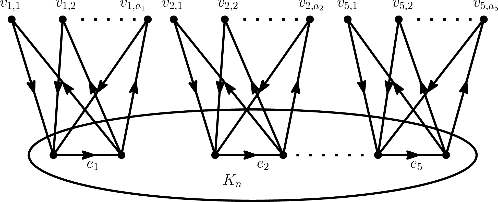
Since \(D_1^\top(G)=n+\sum_{i=1}^{5} a_i\) and \(D_2^\top(G)=n\), it suffices to show that \[\label{eq-m-2} \lambda_1\left(\operatorname{curl}^{*}(G)\operatorname{curl}(G)\right) +\lambda_2\left(\operatorname{curl}^{*}(G)\operatorname{curl}(G)\right) \le 2n+\sum_{i=1}^{5} a_i.\tag{12}\] If \(\lambda_2\left(\operatorname{curl}^{*}(G)\operatorname{curl}(G)\right) \le n= D_2^{\top}(G)\), then we get 12 immediately from Lemma 6. Therefore, it remains to consider the case for \(\lambda_2\left(\operatorname{curl}^{*}(G)\operatorname{curl}(G)\right) > n\), which implies that the operator \(\operatorname{curl}^{*}(G)\operatorname{curl}(G)\) has at least two eigenvalues greater than \(n\).
Let \(\lambda\) be an eigenvalue of \(\operatorname{curl}^{*}(G)\operatorname{curl}(G)\) satisfying \(\lambda>n\). In particular, \(\lambda\) is also an eigenvalue of its matrix representation \(\mathcal{C}^\top (G)\mathcal{C}(G)\). Let \(\mathbf{x}=(x_e)_{e\in E(G)} \in \mathbb{R}^{|E(G)|}\) be a corresponding eigenvector. From the eigenvalue equation \(\left(\mathcal{C}^\top (G)\mathcal{C}(G)\right)\mathbf{x} = \lambda \mathbf{x}\), it follows that, for all \(1\le i\le 5\) and \(1\le j\le a_i\), \[\left\{\begin{matrix} x_{\left\{v_{i,j},e^{-}_i\right\}}+x_{\left\{v_{i,j},e^{+}_i\right\}}+x_{e_i}=\lambda x_{\left\{v_{i,j},e^{-}_i\right\}}, \\[2mm] x_{\left\{v_{i,j},e^{+}_i\right\}}+x_{\left\{v_{i,j},e^{-}_i\right\}}+x_{e_i}=\lambda x_{\left\{v_{i,j},e^{+}_i\right\}}, \end{matrix}\right.\] which immediately implies \[\label{eq-3} x_{\left\{v_{i,j},e^{+}_i\right\}}=x_{\left\{v_{i,j},e^{-}_i\right\}}=\frac{1}{\lambda -2}x_{e_i}.\tag{13}\] Let \(\mathbf{x}_0\) denote the restriction of \(\mathbf{x}\) to \(E(K_n)\). Then \(\mathbf{x}_0\neq \mathbf{0}\), for otherwise \(x_{e_i}=0\) for all \(1\le i\le 5\), and hence \(\mathbf{x}=\mathbf{0}\) by 13 , a contradiction.
Combining 13 with the eigenvalue equation, for all \(1\le i\le 5\), we have \[\label{eq-4} \begin{cases} \frac{\lambda a_i }{\lambda -2}x_{e_{i}} +\left(\mathcal{C}^\top(K_n) \mathcal{C}(K_n)\mathbf{x}_0\right)_{e_i}=\lambda x_{e_{i}}, & 1\le i\le 5,\\[2mm] \left(\mathcal{C}^\top(K_n) \mathcal{C}(K_n)\mathbf{x}_0\right)_{e}=\lambda x_{e}, & e\in E(K_n)\setminus \{e_i\mid 1\le i\le 5\}.\end{cases}\tag{14}\] Noticing that \(\mathcal{B}(K_n)\mathcal{B}^{\top}(K_n)+\mathcal{C}^{\top} (K_n)\mathcal{C}(K_n)=\mathcal{H}(K_n)=nI\), it follows from 14 that \[\label{eq-5} \begin{cases} (\lambda-n)x_{e_{i}}+\left(\mathcal{B}(K_n)\mathcal{B}^{\top}(K_n)\mathbf{x}_0\right)_{e_i}= \frac{\lambda a_i }{\lambda -2}x_{e_{i}}, & 1\le i\le 5,\\[2mm] (\lambda-n)x_{e}+\left(\mathcal{B}(K_n)\mathcal{B}^{\top}(K_n)\mathbf{x}_0\right)_{e}=0, & e\in E(K_n)\setminus \{e_i\mid 1\le i\le 5\}.\end{cases}\tag{15}\] Set \(\mu=\lambda-n>0\) and \(S=\{e_1,e_2,e_3,e_4,e_5\}\). Rearranging the rows and columns so that the edges in \(S\) correspond to the first five indices, 15 can be rewritten as \[\label{eq-6} \bigl(\mu I+\mathcal{B}(K_n)\mathcal{B}^{\top}(K_n)\bigr)\mathbf{x}_0=\frac{\mu+n}{\mu+n-2}A\mathbf{x}_0,\tag{16}\] where \(A=\operatorname{diag}(a_1,a_2,a_3,a_4,a_5,0,\ldots,0).\) Since \(\mu>0\) and \(\mathcal{B}(K_n)\mathcal{B}^{\top}(K_n)\) is positive semi-definite, the matrix \(\mu I+\mathcal{B}(K_n)\mathcal{B}^{\top}(K_n)\) is invertible. Hence, by 16 , we get \[\label{eq-7} \mathbf{x}_0 = \frac{\mu+n}{\mu+n-2} \bigl(\mu I+\mathcal{B}(K_n)\mathcal{B}^{\top}(K_n)\bigr)^{-1} A\mathbf{x}_0.\tag{17}\] It follows from 2 and \(\mathbf{s}\left(\Delta_0(K_n)\right)=\left\{n^{(n-1)},0\right\}\) that the only nonzero eigenvalue of \(\mathcal{B}(K_n)\mathcal{B}^{\top}(K_n)\) is \(n\). Let \(P\) and \(Q\) denote the orthogonal projections, with respect to the standard orthonormal basis, onto the eigenspaces corresponding to the eigenvalues \(n\) and \(0\), respectively. Then \(P+Q=I\), and the spectral decomposition of \(\mathcal{B}(K_n)\mathcal{B}^{\top}(K_n)\) is \[\mathcal{B}(K_n)\mathcal{B}^{\top}(K_n)=nP+0Q=nP.\] Consequently, we have \(\mu I+\mathcal{B}(K_n)\mathcal{B}^{\top}(K_n)=\mu I+nP=(\mu+n)P+\mu Q\), and hence \[\begin{array}{ll} &\bigl(\mu I+\mathcal{B}(K_n)\mathcal{B}^{\top}(K_n))\bigr)^{-1}=\frac{1}{\mu+n}P+\frac{1}{\mu}Q\\[2mm] =&\frac{1}{\mu}I-\frac{n}{\mu(\mu+n)}P=\frac{1}{\mu}I-\frac{1}{\mu(\mu+n)}\mathcal{B}(K_n)\mathcal{B}^{\top}(K_n). \end{array}\] Substituting this into 17 , we obtain \[\label{eq-a-3} \mathbf{x}_0=\frac{\mu+n}{\mu+n-2}\left(\frac{1}{\mu}I-\frac{1}{\mu(\mu+n)}\mathcal{B}(K_n)\mathcal{B}^{\top}(K_n)\right)A\mathbf{x}_0.\tag{18}\] Let \(\mathbf{x}_S=\mathbf{x}_0|_S\) denote the restriction of \(\mathbf{x}_0\) to the coordinates indexed by \(S\). Denote by \(L_S\) and \(A_S\) the principal submatrices of \(\mathcal{B}(K_n)\mathcal{B}^{\top}(K_n)\) and \(A\), respectively, corresponding to the indices in \(S\). From 18 , we get \[\mu\mathbf{x}_S=\left(\frac{\mu+n}{\mu+n-2}A_S-\frac{1}{\mu+n-2}L_SA_S\right)\mathbf{x}_S.\] Multiplying both sides on the left by \(A_S^{1/2}\), we further obtain \[\label{eq-8} \mu A^{\frac{1}{2}}_S\mathbf{x}_S=\left(\frac{\mu+n}{\mu+n-2}A_S-\frac{1}{\mu+n-2}A^{\frac{1}{2}}_SL_SA^{\frac{1}{2}}_S\right)A^{\frac{1}{2}}_S\mathbf{x}_S.\tag{19}\]
Let \(M(x) =\frac{x+n}{x+n-2}A_S-\frac{1}{x+n-2}A_S^{1/2}L_SA_S^{1/2}\). For any \(x>0\), let \(g_1(x)\ge g_2(x)\ge g_3(x)\ge g_4(x)\ge g_5(x)\) denote the eigenvalues of \(M(x)\) arranged in non-increasing order. For \(M(x)\) with \(x>0\), on the one hand, by noticing that \[\begin{align} M(x)&=\frac{x+n}{x+n-2}A_S-\frac{1}{x+n-2}A_S^{1/2}L_SA_S^{1/2} \\&=\frac{x}{x+n-2}A_S+\frac{1}{x+n-2}A_S^{1/2}(nI-L_S)A_S^{1/2}, \end{align}\] we conclude that \(M(x)\) is positive definite since \(nI-L_S\) is positive semidefinite. Thus, \(g_i(x)>0\) for all \(1\le i\le 5\). On the other hand, by noticing that \[\label{eq-10} \begin{align} M(x)&=\frac{x+n}{x+n-2}A_S-\frac{1}{x+n-2}A_S^{1/2}L_SA_S^{1/2} \\&=A_S+\frac{1}{x+n-2}\left(2A_S-A_S^{1/2}L_SA_S^{1/2}\right)\\&=A_S+\frac{1}{x+n-2}A_S^{1/2}\left(2I-L_S\right)A_S^{1/2}, \end{align}\tag{20}\] we get \(\sum_{i=1}^{5}g_i(x)=\operatorname{Tr}(M(x))=\operatorname{Tr}(A_S)=\sum_{i=1}^{5}a_i\) since the diagonal entries of \(2I-L_S\) are \(0\) and \(A_S=\operatorname{diag}(a_1,\ldots,a_5)\) is diagonal. Therefore, for any \(x>0\), we have \[\label{eq-9} g_1(x)+g_2(x)\le \sum_{i=1}^{5}a_i.\tag{21}\]
Equation 19 indicates that \(\mu\) is an eigenvalue of \(M(\mu)\). Hence, there exists \(1\le t\le 5\) such that \(\mu=g_t(\mu)\). For \(i=1,2\), define \(\mu_i=\lambda_i\left(\operatorname{curl}^{*}\operatorname{curl}\right)-n\). Therefore, there exists \(1\le t_i\le 5\) such that \(\mu_i=g_{t_i}(\mu_i)\) for each \(i\in\{1,2\}\), i.e., each \(\mu_i\) can be interpreted as an intersection point of the graphs \(y=x\) and \(y=g_{t_i}(x)\).
Claim 1. \(g_1(x)\) is non-increasing on \((0,\infty)\).
Proof. For each \(x>0\), let \(\mathbf{y}_x\) be a unit eigenvector of \(M(x)\) corresponding to its largest eigenvalue \(g_1(x)\). For any \(\mathbf{z} \in \mathbb{R}^5\) indexed by \(S\), from 20 , we have \[\begin{align} \mathbf{z}^\top M(x)\mathbf{z}&= \mathbf{z}^\top A_S \mathbf{z}+ \frac{2}{x+n-2} \sum_{i<j} \sqrt{a_i a_j}\, \bigl(- (L_S)_{e_i,e_j}\bigr)\, \mathbf{z}_{e_i} \mathbf{z}_{e_j}\\&=\sum_{i=1}^{5}a_i\mathbf{z}_{e_i}^2+ \frac{2}{x+n-2} h(\mathbf{z}), \end{align}\] where \(h(\mathbf{z}) =\sum_{i<j} \sqrt{a_i a_j}\, \bigl(- (L_S)_{e_i,e_j}\bigr)\, \mathbf{z}_{e_i} \mathbf{z}_{e_j}\). To establish that \(g_1(x)\) is non-increasing on \((0,\infty)\), it suffices to show that \(h(\mathbf{y}_x) \ge 0\) for all \(x>0\), where \(\mathbf{y}_x\) is a unit eigenvector of \(M(x)\) corresponding to \(g_1(x)\). Indeed, assuming this, for any \(x_2 \ge x_1 > 0\), \[\begin{align} g_1(x_1) &= \max_{\|\mathbf{z}\|=1} \mathbf{z}^\top M(x_1) \mathbf{z} \ge \mathbf{y}_{x_2}^\top M(x_1) \mathbf{y}_{x_2} \\ &= \mathbf{y}_{x_2}^\top A_S \mathbf{y}_{x_2} + \frac{2}{x_1+n-2} h(\mathbf{y}_{x_2}) \ge \mathbf{y}_{x_2}^\top A_S \mathbf{y}_{x_2} + \frac{2}{x_2+n-2} h(\mathbf{y}_{x_2}) \\ &= \mathbf{y}_{x_2}^\top M(x_2) \mathbf{y}_{x_2} = g_1(x_2), \end{align}\] which implies that \(g_1(x)\) is non-increasing on \((0,\infty)\).
It therefore remains to verify that \(h(\mathbf{y}_x) \ge 0\) for all \(x>0\). Since the verification is technical and tedious, we relegate it to Appendix 5. ◻
If \(\mu_1=\mu_2=\mu\), then they are both eigenvalues of \(M(\mu)\). Therefore, \(\mu_1+\mu_2= g_{t_1}(\mu)+g_{t_2}(\mu)\le g_1(\mu)+g_2(\mu)\le\sum_{i=1}^5a_i\), and thus 12 holds. If \(\mu_1>\mu_2\), then from Claim 1, we have \[\mu_1+\mu_2=g_{t_1}(\mu_1)+g_{t_2}(\mu_2)\le g_{1}(\mu_1)+g_{t_2}(\mu_2)\le g_1(\mu_2)+g_{t_2}(\mu_2)\le \sum_{i=1}^5a_i,\] and thus 12 holds.
This completes the proof. ◻
3.2 Proof of Corollary 1↩︎
From 3 , we obtain that \(\lambda_i(\Delta_1(G))\in \mathbf{s}(\Delta_0(G))\cup \mathbf{s}(\operatorname{curl}^*(G)\operatorname{curl}(G))\) for \(i\in\{1,2\}\). If both \(\lambda_1(\Delta_1(G))\) and \(\lambda_2(\Delta_1(G))\) belong to \(\mathbf{s}\left(\operatorname{curl}^*(G)\operatorname{curl}(G)\right)\), then \[\lambda_i(\Delta_1(G))=\lambda_i(\operatorname{curl}^*(G)\operatorname{curl}(G))\] for \(i\in\{1,2\}\). From Theorem 1, we have \[\lambda_1(\Delta_1(G))+\lambda_2(\Delta_1(G)) \le D_1^\top(G)+D_2^\top(G).\] If neither \(\lambda_1(\Delta_1)\) nor \(\lambda_2(\Delta_1)\) belongs to \(\mathbf{s}\left(\operatorname{curl}^*(G)\operatorname{curl}(G)\right)\), then \(\lambda_i(\Delta_1(G))\in \mathbf{s}(\Delta_0(G))\) for \(i\in\{1,2\}\), and thereby \[\lambda_i(\Delta_1(G))=\lambda_i(\Delta_0(G))\] for \(i\in\{1,2\}\). By a result of Bai [7], we have \[\lambda_1(\Delta_1(G))+\lambda_2(\Delta_1(G)) \le d_1^\top(G)+d_2^\top(G).\] Otherwise, exactly one of \(\lambda_1(\Delta_1(G))\) and \(\lambda_2(\Delta_1(G))\) belongs to \(\mathbf{s}\left(\operatorname{curl}^*(G)\operatorname{curl}(G)\right)\), while the other belongs to \(\mathbf{s}\!\left(\Delta_0(G)\right)\). Then, either \[\lambda_1(\Delta_1(G))=\lambda_1(\Delta_0(G)),\quad\lambda_2(\Delta_1(G))=\lambda_1(\operatorname{curl}^*(G)\operatorname{curl}(G)),\] or \[\lambda_1(\Delta_1(G))=\lambda_1(\operatorname{curl}^*(G)\operatorname{curl}(G)),\quad\lambda_2(\Delta_1(G))=\lambda_1(\Delta_0(G)).\] Therefore, in either case, by Bai’s inequality [7] and 4 , we have \[\lambda_1(\Delta_1(G))+\lambda_2(\Delta_1(G)) \le d_1^\top(G)+D_1^\top(G).\]
This completes the proof.
3.3 Proof of Corollary 2↩︎
The proof proceeds by proving the following two lemmas.
Lemma 10. Let \(K\) be a \(3\)-family on vertex set \(V(K)\) satisfying \(d_2^\top(K)\le 2\). Then \[\lambda_1(\partial_{2}(K)\partial_{2}^*(K)) + \lambda_2(\partial_{2}(K)\partial_{2}^*(K)) \le d_1^\top(K) + d_2^\top(K),\] where \(\partial_{2}(K)\partial_{2}^*(K)\) denotes the up-Laplacian of \(K\).
Proof. Let \(G\) be the graph of \(K\), that is, the graph with vertex set \(V(G)=V(K)\) and edge set \(E(G)\) being all the \(2\)-subsets of a set in \(K\). If \(\triangle=\{i,j,k\}\in T(G)\), then we claim \(\{i,j,k\}\in K\). Otherwise, there exists \(x,y,z\in V(K)\) such that \(\{i,j,x\},\{j,k,y\},\{k,i,z\}\in K\). This leads to \(d_i(K),d_j(K),d_k(K)\ge 2\), and thus \(d_2^T(K)\ge 3\), a contradiction. Hence, \(T(G)\subseteq K\). Conversely, for any set \(\{i,j,k\}\in K\), we obtain that \(\{i,j\},\{j,k\},\{k,i\}\in E(G)\), and thus \(\{i,j,k\}\in T(G)\). Hence, \(K\subseteq T(G)\). This yields \(T(G)=K\). Therefore, we have \(\partial_{2}(K)\partial_{2}^{*}(K)=\operatorname{curl}^*(G)\operatorname{curl}(G)\) and \(D_i^\top(G)=d_i^\top(K)\) for \(i\in\{1,2\}\). It follows from Theorem 1 that \[\begin{array}{lll} &&\lambda_1(\partial_{2}(K)\partial_{2}^*(K)) + \lambda_2(\partial_{2}(K)\partial_{2}^*(K))\\[2mm] &=&\lambda_1\left(\operatorname{curl}^{*}(G)\operatorname{curl}(G)\right)+ \lambda_2\left(\operatorname{curl}^{*}(G)\operatorname{curl}(G)\right)\\[2mm] &\le& D_1^{\top}(G)+D_2^{\top}(G)=d_1^\top(K)+ d_2^\top(K), \end{array}\] as desired. ◻
Lemma 11. Let \(K\) be a \(3\)-family on vertex set \(V(K)\) satisfying \(d_2^\top(K)\ge 3\). Then \[\lambda_1(\partial_{2}(K)\partial_{2}^*(K)) + \lambda_2(\partial_{2}(K)\partial_{2}^*(K)) \le d_1^\top(K) + d_2^\top(K),\] where \(\partial_{2}(K)\partial_{2}^*(K)\) denotes the up-Laplacian of \(K\).
Proof. According to Proposition 6.2 in [8], we have \[\label{eq-t2-1} \lambda_1\!\left(\partial_{2}(K)\partial_{2}^*(K)\right)\le d_1^\top(K).\tag{22}\] Define \[V_1(K) = \left\{v \in V(K) \mid \operatorname{deg}_K(v) = 1\right\}\text{~and~} V_2(K) = \left\{v \in V(K) \mid \operatorname{deg}_K(v) \ge 2\right\}.\] Then \(V(K)=V_1(K)\sqcup V_2(K)\), \(|V(K)|=d_1^\top(K)\) and \(|V_2(K)|=d_2^\top(K)\). We now distinguish two cases and discuss them separately.
Case 1. There is \(\sigma\in K\) such that \(\left|\sigma\cap V_1(K)\right|\ge 2\).
In this case, we proceed by induction on \(|K|\). Since \(d_2^\top(K)\ge 3\), we have \(|K|\ge 3\). If \(|K|=3\), one can verify that \(K\) has the form like \(K=\{\{i,j,k\},\{k,x,y\},\{x,y,z\}\}\), i.e., \(K\cong T(G_4)\) (see Fig. 2). Thus, the result follows immediately from Theorem 1. Next, we consider the case for \(|K|\ge 4\). If \(\lambda_2(\partial_{2}(K)\partial_{2}^*(K))\le 3\), then, by 22 and the assumption \(d_2^\top(K)\ge 3\), we get the result immediately. So, we may assume \(\lambda_2(\partial_{2}(K)\partial_{2}^*(K))\ge 4\). Choose a \(3\)-set \(\sigma\in K\) with \(\left|\sigma\cap V_1(K)\right|\ge 2\). Let \(K'=K\setminus\{\sigma\}\). Since there is no set \(\sigma'\in K'\) with \(|\sigma\cap \sigma'|=2\), we get \[\mathbf{s}\left(\partial_{2}(K)\partial_{2}^*(K)\right)\circ{=}\mathbf{s}\left(\partial_{2}(K')\partial_{2}^*(K')\right)\uplus\{3\}.\] This yields \(\lambda_i(\partial_2(K)\partial_2^*(K))=\lambda_i(\partial_2(K')\partial_2^*(K'))\). Moreover, if \(\left|\sigma\cap V_1(K)\right|=3\), then \(d_1^\top(K')=d_1^\top(K)-3\) and \(d_2^\top(K')=d_2^\top(K)\). If \(\left|\sigma\cap V_1(K)\right|=2\), then we have either \(d_1^\top(K')=d_1^\top(K)-2\) and \(d_2^\top(K')=d_2^\top(K)\), or \(d_1^\top(K')=d_1^\top(K)-1\) and \(d_2^\top(K')=d_2^\top(K)-1\). Thus, we always have \[d_1^\top(K')+d_2^\top(K')\le d_1^\top(K)+d_2^\top(K)-2.\] Note that \(|K'|=|K|-1\). By the induction hypothesis, we get \[\begin{array}{lll} &&\lambda_1\left(\partial_{2}(K)\partial_{2}^*(K)\right)+\lambda_2\left(\partial_{2}(K)\partial_{2}^*(K)\right) \\[2mm] &=&\lambda_1\left(\partial_{2}(K')\partial_{2}^*(K')\right)+\lambda_2\left(\partial_{2}(K')\partial_{2}^*(K')\right)\\[2mm] &\le &d_1^\top(K')+d_2^\top(K')\le d_1^\top(K)+d_2^\top(K)-2, \end{array}\] as desired.
Case 2. For any \(\sigma\in K\), \(\left|\sigma\cap V_1(K)\right|\le 1\).
If \(V_1(K)=\emptyset\), then \(d_1^\top(K)=d_2^\top(K)\). It follows from 22 that \[\lambda_1\!\left(\partial_{2}(K)\partial_{2}^*(K)\right)+\lambda_2\!\left(\partial_{2}(K)\partial_{2}^*(K)\right) \le 2\lambda_1\!\left(\partial_{2}(K)\partial_{2}^*(K)\right) \le 2d_1^\top(K)= d_1^\top(K)+d_2^\top(K),\] as desired. If \(V_1(K)\ne \emptyset\), let \(G\) be the graph of \(K\) as defined in the proof of Lemma 10. Therefore, \(K\subseteq T(G)\) as proved in the proof of Lemma 10. This implies that the matrix representation of \(\partial_2^*(K)\partial_2(K)\) is a principal submatrix of that of \(\partial_2^*(T(G))\partial_2(T(G))\). Hence, by the interlacing theorem and the fact that \(\mathbf{s}(\partial_{2}^*\partial_{2}) \stackrel{\circ}{=} \mathbf{s}(\partial_{2}\partial_{2}^*)\), we have \[\label{eq-thm-z-3} \begin{array}{ll} &\lambda_1(\partial_{2}(K)\partial_{2}^*(K)) + \lambda_2(\partial_{2}(K)\partial_{2}^*(K))\\[2mm] \le& \lambda_1(\partial_{2}(T(G))\partial_{2}^*(T(G))) + \lambda_2(\partial_{2}(T(G))\partial_{2}^*(T(G))). \end{array}\tag{23}\] Recall the definitions of \(V_1(G)\) and \(V_2(G)\) from the second paragraph of Section 3. For the graph \(G\), we have \(V(G)=V(K)\), \(V_1(G)=V_1(K)\) and \(V_2(G)=V_2(K)\), and thus \[\label{eq-thm-z-4} d_1^\top(K)=|V(K)|=|V(G)|=D_1^{\top}(G)\text{ and } d_2^\top(K)=|V_2(K)|=|V_2(G)|=D_2^{\top}(G).\tag{24}\] Since \(\partial_{2}(T(G))\partial_{2}^{*}(T(G))=\operatorname{curl}^*(G)\operatorname{curl}(G)\), it follows from Theorem 1 and 24 that \[\label{eq-thm-z-5} \begin{array}{ll} & \lambda_1(\partial_{2}(T(G))\partial_{2}^*(T(G))) + \lambda_2(\partial_{2}(T(G))\partial_{2}^*(T(G))) \\[2mm] \le & D_1^\top(G) + D_2^\top(G)=d_1^\top(K)+d_2^\top(K). \end{array}\tag{25}\] Therefore, combining 23 with 25 , we have \[\lambda_1\!\left(\partial_{2}(K)\partial_{2}^*(K)\right)+\lambda_2\!\left(\partial_{2}(K)\partial_{2}^*(K)\right) \le d_1^\top(K)+d_2^\top(K).\]
This completes the proof. ◻
Declaration of Interest Statement↩︎
The authors declare that they have no conflicts of interest to this work.
Acknowledgments↩︎
Lu Lu is supported by National Natural Science Foundation of China (No. 12371362). Jianfeng Wang is supported by National Natural Science Foundation of China (No. 12371353).
4 The eigenvalues of graphs in Fig.1↩︎
For \(G\in \left\{t(G)K_3,F_s\cup (t(G)-s)K_3,G_1\right\}\), no two triangles of \(G\) share an edge. Therefore, regardless of the choice of orientation, the matrix representation of \(\operatorname{curl}\operatorname{curl}^*\) is diagonal and equals \[\operatorname{diag}(\underbrace{3,\ldots,3}_{t(G)}).\] Since \(\mathbf{s}(\operatorname{curl}^*\operatorname{curl}) \stackrel{\circ}{=} \mathbf{s}(\operatorname{curl}\operatorname{curl}^*)\) and \(t(G)\ge 2\), we have \[\label{eq-f-1} \lambda_1(\operatorname{curl}^*~\operatorname{curl})+\lambda_2(\operatorname{curl}^*~\operatorname{curl})=6.\tag{26}\] Moreover, if \(G=t(G)K_3\) and \(t(G)\ge 2\), then \[D_1^{\top}(G)+D_2^{\top}(G)=3t(G)\ge 6.\] If \(G=F_s\cup (t(G)-s)K_3\), then \(t(G)\ge s\ge 2\), and thus \[D_1^{\top}(G)+D_2^{\top}(G)=3t(G)-s+1+1\ge 2t(G)+2\ge 6.\] If \(G=G_1\), then \(t(G)\ge \deg_G^{(2)}(u)+\deg_G^{(2)}(v)\ge 4\), and thus \[D_1^{\top}(G)+D_2^{\top}(G)=3t(G)-\deg_G^{(2)}(u)-\deg_G^{(2)}(v)+2\ge 2t(G)+2\ge 6.\] Therefore, in all cases, \[D_1^{\top}(G)+D_2^{\top}(G)\ge 6.\] Combining this with 26 , we obtain \[\lambda_1(\operatorname{curl}^*\operatorname{curl}) + \lambda_2(\operatorname{curl}^*\operatorname{curl}) \le D_1^{\top}(G)+D_2^{\top}(G).\]
For \(G=G_2\), let \[e:=\{u,v\},\qquad d_u:=\deg_G^{(2)}(u),\qquad d_v:=\deg_G^{(2)}(v),\qquad d_e:=\deg_G(e).\] By inclusion–exclusion, we get \(d_u+d_v-d_e\le t(G)\). Hence, \[\label{eq-f-2} D_1^{\top}(G)+D_2^{\top}(G)=3t(G)-(d_u-1)-(d_v-1)+2=3t(G)-d_u-d_v+4\ge 2t(G)-d_e+4.\tag{27}\] Define \[T_1(G)\mid =\{\triangle\in T(G) \mid e\in\triangle\}\text{ and }T_2(G)\mid =T(G)\setminus\{\triangle\in T(G) \mid e\in\triangle\}.\] Since any two triangles in \(T_1(G)\) share the edge \(e\), while no two triangles in \(T_2(G)\) share an edge and no triangle in \(T_1(G)\) shares an edge with a triangle in \(T_2(G)\), the matrix representation \(\mathcal{C}\mathcal{C}^\top\) of \(\operatorname{curl}\operatorname{curl}^*\) is block diagonal. More precisely, after a suitable orientation and ordering of the triangles, we get \[\mathcal{C}\mathcal{C}^\top = \begin{pmatrix} 2I_{d_e}+J_{d_e} & 0\\ 0 & \operatorname{diag}(\underbrace{3,\ldots,3}_{\,t(G)-d_e}) \end{pmatrix},\] where \(J_{d_e}\) denotes the \(d_e\times d_e\) all-ones matrix. Therefore, the non-zero spectrum of \(\operatorname{curl}^*\operatorname{curl}\) is given by \[\label{eq-f-3} \mathbf{s}\left(\operatorname{curl}^*\operatorname{curl}\right)\stackrel{\circ}{=} \mathbf{s}\left(\operatorname{curl}\operatorname{curl}^*\right) \stackrel{\circ}{=} \{d_e+2, 3^{\left(t(G)-d_e\right)}, 2^{(d_e-1)}\}.\tag{28}\] If \(d_e\le t(G)-1\), then \(d_e\le 2t(G)-d_e-2\). Combining this with 27 , we have \[\lambda_1(\operatorname{curl}^*\operatorname{curl})+ \lambda_2(\operatorname{curl}^*\operatorname{curl})=d_e+5\le 2t(G)-d_e+3< 2t(G)-d_e+4\le D_1^{\top}(G)+D_2^{\top}(G).\] Otherwise, \(d_e= t(G)\), and from 27 and 28 , we have \[\lambda_1(\operatorname{curl}^*\operatorname{curl})+ \lambda_2(\operatorname{curl}^*\operatorname{curl})=d_e+4\le D_1^{\top}(G)+D_2^{\top}(G),\] as desired.
5 Non-negativity estimate↩︎
Recall that \(S=\{e_1,e_2,e_3,e_4,e_5\}\), and that \(L_S\) denotes the principal submatrix of \(\mathcal{B}(K_n)\mathcal{B}(K_n)^\top\) induced by \(S\). Moreover, recall that \[\mathbf{z}^\top M(x)\mathbf{z}=\sum_{i=1}^{5} a_i \mathbf{z}_{e_i}^2+\frac{2}{x+n-2} h(\mathbf{z}),\] where \(h(\mathbf{z}):=\sum_{i<j}\sqrt{a_i a_j}\, \bigl(- (L_S)_{e_i,e_j}\bigr)\, \mathbf{z}_{e_i}\mathbf{z}_{e_j}.\) Here \(\mathbf{z} \in \mathbb{R}^5\) is indexed by \(S\), and \(x,a_i>0\) for \(1\le i\le 5\). For each \(x>0\), let \(\mathbf{y}_x\) denote a unit eigenvector of \(M(x)\) corresponding to its largest eigenvalue \(g_1(x)\). In this appendix, we prove that \[h(\mathbf{y}_x) \ge 0 \quad \text{for all } x>0.\]
| Continued from previous page | |||
|---|---|---|---|
| Continued on next page | |||
| (1) | (2) | (3) | (4) |
| (5) | (6) | (7) | (8) |
| (9) | (10) | (11) | (12) |
| (13) | (14) | (15) | (16) |
| (17) | (18) | (19) | (20) |
| (21) | (22) | (23) | (24) |
| (25) | (26) | ||
We now analyze the structure of \(G[S]\). Up to graph isomorphism, there are exactly \(26\) distinct configurations. For each configuration, we proceed as follows.
Choose a suitable orientation for the configuration.
Assume for contradiction that \(h(\mathbf{y}_x)<0\).
Based on the chosen orientation, select a vector \(\mathbf{z}_x\in\mathbb{R}^5\) satisfying \[\|\mathbf{z}_x\|=\|\mathbf{y}_x\|\quad\text{and}\quad \mathbf{z}_x^{\top}M(x)\mathbf{z}_x>\mathbf{y}_x^{\top}M(x)\mathbf{y}_x=g_1(x).\]
This contradicts the fact that \(g_1(x)\) is the largest eigenvalue of \(M(x)\).
We provide the details below.
For the configurations (1), (2), (3), (4), (6), (7), (11), (12), (14), (15), (25).
Since \(\Delta(G[S])\le 2\), there exists an orientation satisfying (i) and (ii) as given in the proof of Lemma 9 such that every pair of adjacent edges in \(S\) is oriented consecutively through their common endpoint (see Table 1). Under this orientation, \((L_S)_{e_i,e_j}\in \{0,-1\}\) for all \(i\ne j\), and thus \(M(x)\) is a nonnegative symmetric matrix for every \(x\ge 0\). Suppose, to the contrary, that \(h(\mathbf{y}_x)<0\). Let \(\mathbf{z}_x=|\mathbf{y}_x|\) be the vector in \(\mathbb{R}^5\) whose components are the absolute values of the corresponding entries of \(\mathbf{y}_x\). Since \[h(\mathbf{z}_x)=\sum_{i<j}\sqrt{a_i a_j}\,\bigl(-(L_S)_{e_i,e_j}\bigr)(\mathbf{z}_x)_{e_i}(\mathbf{z}_x)_{e_j}\ge 0 > h(\mathbf{y}_x),\] and \[\|\mathbf{z}_x\|=\|\mathbf{y}_x\|=1,\qquad \sum_{i=1}^{5} a_i (\mathbf{z}_x)_{e_i}^2=\sum_{i=1}^{5} a_i (\mathbf{y}_x)_{e_i}^2,\] we obtain \[\begin{align} \mathbf{z}_x^{\top}M(x)\mathbf{z}_x &= \sum_{i=1}^{5} a_i (\mathbf{z}_x)_{e_i}^2+\frac{2}{x+n-2}h(\mathbf{z}_x)\\ &> \sum_{i=1}^{5} a_i (\mathbf{y}_x)_{e_i}^2+\frac{2}{x+n-2}h(\mathbf{y}_x)\\ &= \mathbf{y}_x^{\top}M(x)\mathbf{y}_x= g_1(x). \end{align}\]
For the configurations (5).
We fix an orientation satisfying (i) and (ii) such that the edges in \(S\) are oriented as depicted in Table 1. Under this orientation, for any \(x>0\), \[h(\mathbf{y}_x) = \sqrt{a_{i_3}a_{i_5}}(\mathbf{y}_x)_{e_{i_3}}(\mathbf{y}_x)_{e_{i_5}} +\sqrt{a_{i_4}a_{i_5}}(\mathbf{y}_x)_{e_{i_4}}(\mathbf{y}_x)_{e_{i_5}} -\sqrt{a_{i_3}a_{i_4}}(\mathbf{y}_x)_{e_{i_3}}(\mathbf{y}_x)_{e_{i_4}}.\] Suppose, to the contrary, that \(h(\mathbf{y}_x)<0\). If \[\sqrt{a_{i_5}}\bigl|(\mathbf{y}_x)_{e_{i_5}}\bigr|= \max_{j\in\{3,4,5\}} \sqrt{a_{i_j}}\bigl|(\mathbf{y}_x)_{e_{i_j}}\bigr|,\] set \(\mathbf{z}_x=|\mathbf{y}_x|\). Otherwise, let \(t\in\{3,4\}\) such that \[\sqrt{a_{i_t}}\bigl|(\mathbf{y}_x)_{e_{i_t}}\bigr|= \max_{j\in\{3,4,5\}} \sqrt{a_{i_j}}\bigl|(\mathbf{y}_x)_{e_{i_j}}\bigr|,\] and define \(\mathbf{z}_x\in\mathbb{R}^5\) by \[(\mathbf{z}_x)_{e_{i_j}}=\begin{cases} -\bigl|(\mathbf{y}_x)_{e_{i_j}}\bigr|, & j\in \{t,5\},\\ \bigl|(\mathbf{y}_x)_{e_{i_j}}\bigr|, &\text{ otherwise}. \end{cases}\] In either case, \[h(\mathbf{z}_x)\ge0>h(\mathbf{y}_x),\] while \[\|\mathbf{z}_x\|=\|\mathbf{y}_x\|=1,\qquad\sum_{i=1}^{5} a_i (\mathbf{z}_x)_{e_i}^2=\sum_{i=1}^{5} a_i (\mathbf{y}_x)_{e_i}^2.\] Consequently, \[\begin{align}\mathbf{z}_x^{\top}M(x)\mathbf{z}_x &= \sum_{i=1}^{5} a_i (\mathbf{z}_x)_{e_i}^2+\frac{2}{x+n-2}h(\mathbf{z}_x)\\ &>\sum_{i=1}^{5} a_i (\mathbf{y}_x)_{e_i}^2+\frac{2}{x+n-2}h(\mathbf{y}_x)\\ &=\mathbf{y}_x^{\top}M(x)\mathbf{y}_x\\ &=g_1(x).\end{align}\]
For the configurations (8).
We fix an orientation satisfying (i) and (ii) such that the edges in \(S\) are oriented as depicted in Table 1. Under this orientation, for any \(x>0\), \[\begin{array}{lll} h(\mathbf{y}_x) &=& \sqrt{a_{i_2}a_{i_3}}(\mathbf{y}_x)_{e_{i_2}}(\mathbf{y}_x)_{e_{i_3}} +\sqrt{a_{i_3}a_{i_4}}(\mathbf{y}_x)_{e_{i_3}}(\mathbf{y}_x)_{e_{i_4}}\\[2mm] &&+\sqrt{a_{i_3}a_{i_5}}(\mathbf{y}_x)_{e_{i_3}}(\mathbf{y}_x)_{e_{i_5}} -\sqrt{a_{i_4}a_{i_5}}(\mathbf{y}_x)_{e_{i_4}}(\mathbf{y}_x)_{e_{i_5}}. \end{array}\] Suppose, to the contrary, that \(h(\mathbf{y}_x)<0\). If \[\sqrt{a_{i_3}}\bigl|(\mathbf{y}_x)_{e_{i_3}}\bigr|=\max_{j\in\{3,4,5\}} \sqrt{a_{i_j}}\bigl|(\mathbf{y}_x)_{e_{i_j}}\bigr|,\] set \(\mathbf{z}_x:=|\mathbf{y}_x|\). Otherwise, let \(t\in\{4,5\}\) such that \[\sqrt{a_{i_t}}\bigl|(\mathbf{y}_x)_{e_{i_t}}\bigr|=\max_{j\in\{3,4,5\}} \sqrt{a_{i_j}}\bigl|(\mathbf{y}_x)_{e_{i_j}}\bigr|,\] and define \(\mathbf{z}_x\in\mathbb{R}^5\) by \[(\mathbf{z}_x)_{e_{i_j}}=\begin{cases} -|(\mathbf{y}_x)_{e_{i_j}}|, & j\in\{t,2,3\},\\ |(\mathbf{y}_x)_{e_{i_j}}|, & \text{ otherwise}. \end{cases}\] In either case, \[h(\mathbf{z}_x)\ge0>h(\mathbf{y}_x),\] while \[\|\mathbf{z}_x\|=\|\mathbf{y}_x\|=1,\qquad\sum_{i=1}^{5} a_i (\mathbf{z}_x)_{e_i}^2=\sum_{i=1}^{5} a_i (\mathbf{y}_x)_{e_i}^2.\] Consequently, \[\begin{align}\mathbf{z}_x^{\top}M(x)\mathbf{z}_x &= \sum_{i=1}^{5} a_i (\mathbf{z}_x)_{e_i}^2+\frac{2}{x+n-2}h(\mathbf{z}_x)\\ &>\sum_{i=1}^{5} a_i (\mathbf{y}_x)_{e_i}^2+\frac{2}{x+n-2}h(\mathbf{y}_x)\\ &=\mathbf{y}_x^{\top}M(x)\mathbf{y}_x\\ &=g_1(x).\end{align}\]
For the configurations (9).
We fix an orientation satisfying (i) and (ii) such that the edges in \(S\) are oriented as shown in Table 1. Under this orientation, \[\begin{align} h(\mathbf{y}_x) &=\sqrt{a_{i_1}a_{i_3}}\,(\mathbf{y}_x)_{e_{i_1}}(\mathbf{y}_x)_{e_{i_3}}+\sqrt{a_{i_1}a_{i_2}}\,(\mathbf{y}_x)_{e_{i_1}}(\mathbf{y}_x)_{e_{i_2}} +\sqrt{a_{i_1}a_{i_4}}\,(\mathbf{y}_x)_{e_{i_1}}(\mathbf{y}_x)_{e_{i_4}} \\&\quad-\sqrt{a_{i_2}a_{i_3}}\,(\mathbf{y}_x)_{e_{i_2}}(\mathbf{y}_x)_{e_{i_3}}-\sqrt{a_{i_2}a_{i_4}}\,(\mathbf{y}_x)_{e_{i_2}}(\mathbf{y}_x)_{e_{i_4}}-\sqrt{a_{i_3}a_{i_4}}\,(\mathbf{y}_x)_{e_{i_3}}(\mathbf{y}_x)_{e_{i_4}}. \end{align}\] Suppose, to the contrary, that \(h(\mathbf{y}_x)<0\). If \[\sqrt{a_{i_1}}\bigl|(\mathbf{y}_x)_{e_{i_1}}\bigr|=\max_{j\in\{1,2,3,4\}}\sqrt{a_{i_j}}\bigl|(\mathbf{y}_x)_{e_{i_j}}\bigr|,\] then set \(\mathbf{z}_x\mid =|\mathbf{y}_x|\). Otherwise, let \(t\in\{2,3,4\}\) such that \[\sqrt{a_{i_t}}\bigl|(\mathbf{y}_x)_{e_{i_t}}\bigr|=\max_{j\in\{1,2,3,4\}}\sqrt{a_{i_j}}\bigl|(\mathbf{y}_x)_{e_{i_j}}\bigr|,\] and define \(\mathbf{z}_x\in\mathbb{R}^5\) by \[(\mathbf{z}_x)_{e_{i_j}}=\begin{cases} -|(\mathbf{y}_x)_{e_{i_j}}|, & j\in \{1,t\},\\[1mm] |(\mathbf{y}_x)_{e_{i_j}}|, & \text{otherwise}. \end{cases}\] A direct verification shows that, in each of the above cases, \(h(\mathbf{z}_x)\ge 0>h(\mathbf{y}_x)\). Moreover, since \(\|\mathbf{z}_x\|=\|\mathbf{y}_x\|=1\) and \(\sum_{i=1}^{5} a_i (\mathbf{z}_x)_{e_i}^2=\sum_{i=1}^{5} a_i (\mathbf{y}_x)_{e_i}^2\), we \[\begin{align}\mathbf{z}_x^{\top}M(x)\mathbf{z}_x &= \sum_{i=1}^{5} a_i (\mathbf{z}_x)_{e_i}^2+\frac{2}{x+n-2}h(\mathbf{z}_x)\\ &>\sum_{i=1}^{5} a_i (\mathbf{y}_x)_{e_i}^2+\frac{2}{x+n-2}h(\mathbf{y}_x)\\ &=\mathbf{y}_x^{\top}M(x)\mathbf{y}_x\\ &=g_1(x).\end{align}\]
For the configurations (10).
We fix an orientation satisfying (i) and (ii) such that the edges in \(S\) are oriented as depicted in Table 1. Under this orientation, for any \(x>0\), \[\begin{align} h(\mathbf{y}_x) &= \sqrt{a_{i_2}a_{i_3}}\, (\mathbf{y}_x)_{e_{i_2}} (\mathbf{y}_x)_{e_{i_3}} + \sqrt{a_{i_3}a_{i_4}}\, (\mathbf{y}_x)_{e_{i_3}} (\mathbf{y}_x)_{e_{i_4}}+ \sqrt{a_{i_2}a_{i_4}}\, (\mathbf{y}_x)_{e_{i_2}} (\mathbf{y}_x)_{e_{i_4}} \\ &\quad + \sqrt{a_{i_1}a_{i_4}}\, (\mathbf{y}_x)_{e_{i_1}} (\mathbf{y}_x)_{e_{i_4}}- \sqrt{a_{i_1}a_{i_2}}\, (\mathbf{y}_x)_{e_{i_1}} (\mathbf{y}_x)_{e_{i_2}}. \end{align}\] Suppose, to the contrary, that \(h(\mathbf{y}_x)<0\). If \[\sqrt{a_{i_4}}\bigl|(\mathbf{y}_x)_{e_{i_4}}\bigr|\ge \sqrt{a_{i_2}}\bigl|(\mathbf{y}_x)_{e_{i_2}}\bigr|,\] then set \(\mathbf{z}_x:=|\mathbf{y}_x|\). Otherwise, define \(\mathbf{z}_x\in\mathbb{R}^5\) by \[(\mathbf{z}_x)_{e_{i_j}}=\begin{cases}-|(\mathbf{y}_x)_{e_{i_j}}|, & j=1\\|(\mathbf{y}_x)_{e_{i_j}}|, & \text{otherwise}. \end{cases}\] In either case, \[h(\mathbf{z}_x)\ge0>h(\mathbf{y}_x),\] while \[\|\mathbf{z}_x\|=\|\mathbf{y}_x\|=1,\qquad\sum_{i=1}^{5} a_i (\mathbf{z}_x)_{e_i}^2=\sum_{i=1}^{5} a_i (\mathbf{y}_x)_{e_i}^2.\] Consequently, \[\begin{align}\mathbf{z}_x^{\top}M(x)\mathbf{z}_x &= \sum_{i=1}^{5} a_i (\mathbf{z}_x)_{e_i}^2+\frac{2}{x+n-2}h(\mathbf{z}_x)\\ &>\sum_{i=1}^{5} a_i (\mathbf{y}_x)_{e_i}^2+\frac{2}{x+n-2}h(\mathbf{y}_x)\\ &=\mathbf{y}_x^{\top}M(x)\mathbf{y}_x\\ &=g_1(x).\end{align}\]
For the configurations (13).
We fix an orientation satisfying (i) and (ii) such that the edges in \(S\) are oriented as depicted in Table 1. Under this orientation, for any \(x>0\), \[\begin{align} h(\mathbf{y}_x) &= \sqrt{a_{i_1}a_{i_2}}\, (\mathbf{y}_x)_{e_{i_1}} (\mathbf{y}_x)_{e_{i_2}}+ \sqrt{a_{i_1}a_{i_3}}\, (\mathbf{y}_x)_{e_{i_1}} (\mathbf{y}_x)_{e_{i_3}}+ \sqrt{a_{i_4}a_{i_5}}\, (\mathbf{y}_x)_{e_{i_4}} (\mathbf{y}_x)_{e_{i_5}} \\ &\quad -\sqrt{a_{i_2}a_{i_3}}\, (\mathbf{y}_x)_{e_{i_2}} (\mathbf{y}_x)_{e_{i_3}}. \end{align}\] Suppose, to the contrary, that \(h(\mathbf{y}_x)<0\). If \[\sqrt{a_{i_1}}\bigl|(\mathbf{y}_x)_{e_{i_1}}\bigr|=\max_{j\in\{1,2,3\}}\sqrt{a_{i_j}}\bigl|(\mathbf{y}_x)_{e_{i_j}}\bigr|,\] set \(\mathbf{z}_x:=|\mathbf{y}_x|\). Otherwise, let \(t\in \{2,3\}\) such that \[\sqrt{a_{i_t}}\bigl|(\mathbf{y}_x)_{e_{i_t}}\bigr|=\max_{j\in\{1,2,3\}}\sqrt{a_{i_j}}\bigl|(\mathbf{y}_x)_{e_{i_j}}\bigr|,\] and define \(\mathbf{z}_x\in\mathbb{R}^5\) by \[(\mathbf{z}_x)_{e_{i_j}}=\begin{cases} -|(\mathbf{y}_x)_{e_{i_j}}|, & j=\{1,t\}\\ |(\mathbf{y}_x)_{e_{i_j}}|, &\text{otherwise}.\end{cases}\] In either case, \[h(\mathbf{z}_x)\ge0>h(\mathbf{y}_x),\] while \[\|\mathbf{z}_x\|=\|\mathbf{y}_x\|=1,\qquad\sum_{i=1}^{5} a_i (\mathbf{z}_x)_{e_i}^2=\sum_{i=1}^{5} a_i (\mathbf{y}_x)_{e_i}^2.\] Consequently, \[\begin{align}\mathbf{z}_x^{\top}M(x)\mathbf{z}_x &= \sum_{i=1}^{5} a_i (\mathbf{z}_x)_{e_i}^2+\frac{2}{x+n-2}h(\mathbf{z}_x)\\ &>\sum_{i=1}^{5} a_i (\mathbf{y}_x)_{e_i}^2+\frac{2}{x+n-2}h(\mathbf{y}_x)\\ &=\mathbf{y}_x^{\top}M(x)\mathbf{y}_x\\ &=g_1(x).\end{align}\]
For the configurations (16).
We fix an orientation satisfying (i) and (ii) such that the edges in \(S\) are oriented as depicted in Table 1. Under this orientation, for any \(x>0\), \[\begin{align} h(\mathbf{y}_x) &= \sqrt{a_{i_2}a_{i_3}}\, (\mathbf{y}_x)_{e_{i_2}} (\mathbf{y}_x)_{e_{i_3}}+ \sqrt{a_{i_1}a_{i_3}}\, (\mathbf{y}_x)_{e_{i_1}} (\mathbf{y}_x)_{e_{i_3}}+ \sqrt{a_{i_4}a_{i_5}}\, (\mathbf{y}_x)_{e_{i_4}} (\mathbf{y}_x)_{e_{i_5}} \\ &\quad + \sqrt{a_{i_3}a_{i_4}}\, (\mathbf{y}_x)_{e_{i_3}} (\mathbf{y}_x)_{e_{i_4}}-\sqrt{a_{i_1}a_{i_2}}\, (\mathbf{y}_x)_{e_{i_1}} (\mathbf{y}_x)_{e_{i_2}}. \end{align}\] Suppose, to the contrary, that \(h(\mathbf{y}_x)<0\). If \[\sqrt{a_{i_3}}\bigl|(\mathbf{y}_x)_{e_{i_3}}\bigr|=\max_{j\in\{1,2,3\}}\sqrt{a_{i_j}}\bigl|(\mathbf{y}_x)_{e_{i_j}}\bigr|,\] set \(\mathbf{z}_x:=|\mathbf{y}_x|\). Otherwise, let \(t\in \{1,3\}\) such that \[\sqrt{a_{i_t}}\bigl|(\mathbf{y}_x)_{e_{i_t}}\bigr|=\max_{j\in\{1,2,3\}}\sqrt{a_{i_j}}\bigl|(\mathbf{y}_x)_{e_{i_j}}\bigr|,\] and define \(\mathbf{z}_x\in\mathbb{R}^5\) by \[(\mathbf{z}_x)_{e_{i_j}}=\begin{cases}-|(\mathbf{y}_x)_{e_{i_j}}|, & j\in \{3,4,5,t\},\\|(\mathbf{y}_x)_{e_{i_j}}|, & \text{otherwise}. \end{cases}\] In either case, \[h(\mathbf{z}_x)\ge0>h(\mathbf{y}_x),\] while \[\|\mathbf{z}_x\|=\|\mathbf{y}_x\|=1,\qquad\sum_{i=1}^{5} a_i (\mathbf{z}_x)_{e_i}^2=\sum_{i=1}^{5} a_i (\mathbf{y}_x)_{e_i}^2.\] Consequently, \[\begin{align}\mathbf{z}_x^{\top}M(x)\mathbf{z}_x &= \sum_{i=1}^{5} a_i (\mathbf{z}_x)_{e_i}^2+\frac{2}{x+n-2}h(\mathbf{z}_x)\\ &>\sum_{i=1}^{5} a_i (\mathbf{y}_x)_{e_i}^2+\frac{2}{x+n-2}h(\mathbf{y}_x)\\ &=\mathbf{y}_x^{\top}M(x)\mathbf{y}_x\\ &=g_1(x).\end{align}\]
For the configurations (17).
We fix an orientation satisfying (i) and (ii) such that the edges in \(S\) are oriented as depicted in Table 1. Under this orientation, for any \(x>0\), \[\begin{align} h(\mathbf{y}_x) &=\sqrt{a_{i_4}a_{i_5}}\, (\mathbf{y}_x)_{e_{i_4}} (\mathbf{y}_x)_{e_{i_5}}+\sqrt{a_{i_2}a_{i_4}}\, (\mathbf{y}_x)_{e_{i_2}} (\mathbf{y}_x)_{e_{i_4}}+ \sqrt{a_{i_2}a_{i_3}}\, (\mathbf{y}_x)_{e_{i_2}} (\mathbf{y}_x)_{e_{i_3}} \\ &\quad + \sqrt{a_{i_1}a_{i_4}}\, (\mathbf{y}_x)_{e_{i_1}} (\mathbf{y}_x)_{e_{i_4}} -\sqrt{a_{i_1}a_{i_2}}\, (\mathbf{y}_x)_{e_{i_1}} (\mathbf{y}_x)_{e_{i_2}}. \end{align}\] Suppose, to the contrary, that \(h(\mathbf{y}_x)<0\). If \[\sqrt{a_{i_4}}\bigl|(\mathbf{y}_x)_{e_{i_4}}\bigr| \neq \min_{j\in\{1,2,4\}} \sqrt{a_{i_j}}\bigl|(\mathbf{y}_x)_{e_{i_j}}\bigr|,\] set \(\mathbf{z}_x:=|\mathbf{y}_x|\). Otherwise, define \(\mathbf{z}_x\in\mathbb{R}^5\) by \[(\mathbf{z}_x)_{e_{i_j}}= \begin{cases} -|(\mathbf{y}_x)_{e_{i_j}}|, & j=1\\ |(\mathbf{y}_x)_{e_{i_j}}|, &\text{otherwise}. \end{cases}\] In either case, \[h(\mathbf{z}_x)\ge0>h(\mathbf{y}_x),\] while \[\|\mathbf{z}_x\|=\|\mathbf{y}_x\|=1,\qquad\sum_{i=1}^{5} a_i (\mathbf{z}_x)_{e_i}^2=\sum_{i=1}^{5} a_i (\mathbf{y}_x)_{e_i}^2.\] Consequently, \[\begin{align}\mathbf{z}_x^{\top}M(x)\mathbf{z}_x &= \sum_{i=1}^{5} a_i (\mathbf{z}_x)_{e_i}^2+\frac{2}{x+n-2}h(\mathbf{z}_x)\\ &>\sum_{i=1}^{5} a_i (\mathbf{y}_x)_{e_i}^2+\frac{2}{x+n-2}h(\mathbf{y}_x)\\ &=\mathbf{y}_x^{\top}M(x)\mathbf{y}_x\\ &=g_1(x).\end{align}\]
For the configurations (18).
We fix an orientation satisfying (i) and (ii) such that the edges in \(S\) are oriented as depicted in Table 1. Under this orientation, for any \(x>0\), \[\begin{align} h(\mathbf{y}_x) &=\sqrt{a_{i_2}a_{i_5}}\, (\mathbf{y}_x)_{e_{i_2}} (\mathbf{y}_x)_{e_{i_5}}+\sqrt{a_{i_2}a_{i_4}}\, (\mathbf{y}_x)_{e_{i_2}} (\mathbf{y}_x)_{e_{i_4}}+ \sqrt{a_{i_2}a_{i_3}}\, (\mathbf{y}_x)_{e_{i_2}} (\mathbf{y}_x)_{e_{i_3}} \\ &\quad +\sqrt{a_{i_1}a_{i_2}}\, (\mathbf{y}_x)_{e_{i_1}} (\mathbf{y}_x)_{e_{i_2}} + \sqrt{a_{i_1}a_{i_4}}\, (\mathbf{y}_x)_{e_{i_1}} (\mathbf{y}_x)_{e_{i_4}} -\sqrt{a_{i_1}a_{i_5}}\, (\mathbf{y}_x)_{e_{i_1}} (\mathbf{y}_x)_{e_{i_5}} \\ &\quad - \sqrt{a_{i_3}a_{i_4}}\, (\mathbf{y}_x)_{e_{i_3}} (\mathbf{y}_x)_{e_{i_4}} . \end{align}\] We claim that \(h(\mathbf{y}_x)\ge0\). Suppose, to the contrary, that \(h(\mathbf{y}_x)<0\). If \[\sqrt{a_{i_2}}\bigl|(\mathbf{y}_x)_{e_{i_2}}\bigr|=\max_{j\in\{1,2,5\}}\sqrt{a_{i_j}}\bigl|(\mathbf{y}_x)_{e_{i_j}}\bigr|=\max_{j\in\{2,3,4\}}\sqrt{a_{i_j}}\bigl|(\mathbf{y}_x)_{e_{i_j}}\bigr|,\] then set \(\mathbf{z}_x:=|\mathbf{y}_x|\). If \[\sqrt{a_{i_2}}\bigl|(\mathbf{y}_x)_{e_{i_2}}\bigr|\ne\max_{j\in\{1,2,5\}}\sqrt{a_{i_j}}\bigl|(\mathbf{y}_x)_{e_{i_j}}\bigr|\ne \max_{j\in\{2,3,4\}}\sqrt{a_{i_j}}\bigl|(\mathbf{y}_x)_{e_{i_j}}\bigr|,\] then let \(t_1\in \{1,5\}\) and \(t_2\in \{3,4\}\) such that \[\sqrt{a_{i_{t_1}}}\bigl|(\mathbf{y}_x)_{e_{i_{t_1}}}\bigr|=\max_{j\in\{1,2,5\}}\sqrt{a_{i_j}}\bigl|(\mathbf{y}_x)_{e_{i_j}}\bigr|\text{ and }\sqrt{a_{i_{t_2}}}\bigl|(\mathbf{y}_x)_{e_{i_{t_2}}}\bigr|=\max_{j\in\{2,3,4\}}\sqrt{a_{i_j}}\bigl|(\mathbf{y}_x)_{e_{i_j}}\bigr|.\] Define \(\mathbf{z}_x\in\mathbb{R}^5\) by \[(\mathbf{z}_x)_{e_{i_j}}= \begin{cases} -|(\mathbf{y}_x)_{e_{i_j}}|, & j\in \{1,3,4,5\}\setminus\{t_1,t_2\}\\ |(\mathbf{y}_x)_{e_{i_j}}|, & \text{otherwise}. \end{cases}\] If \[\sqrt{a_{i_2}}\bigl|(\mathbf{y}_x)_{e_{i_2}}\bigr|=\max_{j\in\{1,2,5\}}\sqrt{a_{i_j}}\bigl|(\mathbf{y}_x)_{e_{i_j}}\bigr|\ne \max_{j\in\{2,3,4\}}\sqrt{a_{i_j}}\bigl|(\mathbf{y}_x)_{e_{i_j}}\bigr|,\] then let \(t_2\in \{3,4\}\) such that \[\sqrt{a_{i_{t_2}}}\bigl|(\mathbf{y}_x)_{e_{i_{t_2}}}\bigr|=\max_{j\in\{2,3,4\}}\sqrt{a_{i_j}}\bigl|(\mathbf{y}_x)_{e_{i_j}}\bigr|,\] and define \(\mathbf{z}_x\in\mathbb{R}^5\) by \[(\mathbf{z}_x)_{e_{i_j}}= \begin{cases} -|(\mathbf{y}_x)_{e_{i_j}}|, & j\in \{3,4\}\setminus\{t_2\}\\ |(\mathbf{y}_x)_{e_{i_j}}|, & \text{otherwise}. \end{cases}\] If \[\sqrt{a_{i_2}}\bigl|(\mathbf{y}_x)_{e_{i_2}}\bigr|= \max_{j\in\{2,3,4\}}\sqrt{a_{i_j}}\bigl|(\mathbf{y}_x)_{e_{i_j}}\bigr|\ne \max_{j\in\{1,2,5\}}\sqrt{a_{i_j}}\bigl|(\mathbf{y}_x)_{e_{i_j}}\bigr|,\] then let \(t_1\in \{1,5\}\) such that \[\sqrt{a_{i_{t_1}}}\bigl|(\mathbf{y}_x)_{e_{i_{t_1}}}\bigr|=\max_{j\in\{1,2,5\}}\sqrt{a_{i_j}}\bigl|(\mathbf{y}_x)_{e_{i_j}}\bigr|,\] and define \(\mathbf{z}_x\in\mathbb{R}^5\) by \[(\mathbf{z}_x)_{e_{i_j}}= \begin{cases} -|(\mathbf{y}_x)_{e_{i_j}}|, & j\in \{1,5\}\setminus\{t_1\}\\ |(\mathbf{y}_x)_{e_{i_j}}|, & \text{otherwise}. \end{cases}\] In all cases, \[h(\mathbf{z}_x)\ge0>h(\mathbf{y}_x),\] while \[\|\mathbf{z}_x\|=\|\mathbf{y}_x\|=1,\qquad\sum_{i=1}^{5} a_i (\mathbf{z}_x)_{e_i}^2=\sum_{i=1}^{5} a_i (\mathbf{y}_x)_{e_i}^2.\] Consequently, \[\begin{align}\mathbf{z}_x^{\top}M(x)\mathbf{z}_x &= \sum_{i=1}^{5} a_i (\mathbf{z}_x)_{e_i}^2+\frac{2}{x+n-2}h(\mathbf{z}_x)\\ &>\sum_{i=1}^{5} a_i (\mathbf{y}_x)_{e_i}^2+\frac{2}{x+n-2}h(\mathbf{y}_x)\\ &=\mathbf{y}_x^{\top}M(x)\mathbf{y}_x\\ &=g_1(x).\end{align}\]
For the configurations (19).
We fix an orientation satisfying (i) and (ii) such that the edges in \(S\) are oriented as depicted in Table 1. Under this orientation, for any \(x>0\), \[\begin{align} h(\mathbf{y}_x) &= \sqrt{a_{i_2}a_{i_3}}\, (\mathbf{y}_x)_{e_{i_2}} (\mathbf{y}_x)_{e_{i_3}}+ \sqrt{a_{i_3}a_{i_4}}\, (\mathbf{y}_x)_{e_{i_3}} (\mathbf{y}_x)_{e_{i_4}}+ \sqrt{a_{i_1}a_{i_4}}\, (\mathbf{y}_x)_{e_{i_1}} (\mathbf{y}_x)_{e_{i_4}} \\ &\quad + \sqrt{a_{i_1}a_{i_3}}\, (\mathbf{y}_x)_{e_{i_1}} (\mathbf{y}_x)_{e_{i_3}}+ \sqrt{a_{i_2}a_{i_5}}\, (\mathbf{y}_x)_{e_{i_2}} (\mathbf{y}_x)_{e_{i_5}} -\sqrt{a_{i_1}a_{i_2}}\, (\mathbf{y}_x)_{e_{i_1}} (\mathbf{y}_x)_{e_{i_2}}. \end{align}\] Suppose, to the contrary, that \(h(\mathbf{y}_x)<0\). If \[\sqrt{a_{i_3}}\bigl|(\mathbf{y}_x)_{e_{i_3}}\bigr|\ge \sqrt{a_{i_1}}\bigl|(\mathbf{y}_x)_{e_{i_1}}\bigr|\] set \(\mathbf{z}_x:=|\mathbf{y}_x|\). Otherwise, define \(\mathbf{z}_x\in\mathbb{R}^5\) by \[(\mathbf{z}_x)_{e_{i_j}} =\begin{cases} -|(\mathbf{y}_x)_{e_{i_j}}|, & j\in\{1,3,4\}\\ |(\mathbf{y}_x)_{e_{i_j}}|, & \text{ otherwise}. \end{cases}\] In either case, \[h(\mathbf{z}_x)\ge0>h(\mathbf{y}_x),\] while \[\|\mathbf{z}_x\|=\|\mathbf{y}_x\|=1,\qquad\sum_{i=1}^{5} a_i (\mathbf{z}_x)_{e_i}^2=\sum_{i=1}^{5} a_i (\mathbf{y}_x)_{e_i}^2.\] \[\begin{align}\mathbf{z}_x^{\top}M(x)\mathbf{z}_x &= \sum_{i=1}^{5} a_i (\mathbf{z}_x)_{e_i}^2+\frac{2}{x+n-2}h(\mathbf{z}_x)\\ &>\sum_{i=1}^{5} a_i (\mathbf{y}_x)_{e_i}^2+\frac{2}{x+n-2}h(\mathbf{y}_x)\\ &=\mathbf{y}_x^{\top}M(x)\mathbf{y}_x\\ &=g_1(x).\end{align}\]
For the configurations (20).
We fix an orientation satisfying (i) and (ii) such that the edges in \(S\) are oriented as depicted in Table 1. Under this orientation, for any \(x>0\), \[\begin{align} h(\mathbf{y}_x) &=\sqrt{a_{i_1}a_{i_5}}\, (\mathbf{y}_x)_{e_{i_1}} (\mathbf{y}_x)_{e_{i_5}} ++\sqrt{a_{i_1}a_{i_4}}\, (\mathbf{y}_x)_{e_{i_1}} (\mathbf{y}_x)_{e_{i_4}} + \sqrt{a_{i_4}a_{i_5}}\, (\mathbf{y}_x)_{e_{i_4}} (\mathbf{y}_x)_{e_{i_5}}\\ &\quad + \sqrt{a_{i_2}a_{i_5}}\, (\mathbf{y}_x)_{e_{i_2}} (\mathbf{y}_x)_{e_{i_5}}+\sqrt{a_{i_3}a_{i_4}}\, (\mathbf{y}_x)_{e_{i_3}} (\mathbf{y}_x)_{e_{i_4}}-\sqrt{a_{i_1}a_{i_3}}\, (\mathbf{y}_x)_{e_{i_1}} (\mathbf{y}_x)_{e_{i_3}} \\ &\quad -\sqrt{a_{i_1}a_{i_2}}\, (\mathbf{y}_x)_{e_{i_1}} (\mathbf{y}_x)_{e_{i_2}}. \end{align}\] Suppose, to the contrary, that \(h(\mathbf{y}_x)<0\). If \[\sqrt{a_{i_4}}\bigl|(\mathbf{y}_x)_{e_{i_4}}\bigr|+\sqrt{a_{i_5}}\bigl|(\mathbf{y}_x)_{e_{i_5}}\bigr|\ge \sqrt{a_{i_2}}\bigl|(\mathbf{y}_x)_{e_{i_2}}\bigr|+\sqrt{a_{i_3}}\bigl|(\mathbf{y}_x)_{e_{i_3}}\bigr|,\] then set \(\mathbf{z}_x:=|\mathbf{y}_x|\). Otherwise, define \(\mathbf{z}_x\in\mathbb{R}^5\) by \[(\mathbf{z}_x)_{e_{i_j}}=\begin{cases} -|(\mathbf{y}_x)_{e_{i_j}}|, & j=1\\ |(\mathbf{y}_x)_{e_{i_j}}|, & \text{otherwise}. \end{cases}\] In either case, \[h(\mathbf{z}_x)\ge0>h(\mathbf{y}_x),\] while \[\|\mathbf{z}_x\|=\|\mathbf{y}_x\|=1,\qquad\sum_{i=1}^{5} a_i (\mathbf{z}_x)_{e_i}^2=\sum_{i=1}^{5} a_i (\mathbf{y}_x)_{e_i}^2.\] Consequently, \[\begin{align}\mathbf{z}_x^{\top}M(x)\mathbf{z}_x &= \sum_{i=1}^{5} a_i (\mathbf{z}_x)_{e_i}^2+\frac{2}{x+n-2}h(\mathbf{z}_x)\\ &>\sum_{i=1}^{5} a_i (\mathbf{y}_x)_{e_i}^2+\frac{2}{x+n-2}h(\mathbf{y}_x)\\ &=\mathbf{y}_x^{\top}M(x)\mathbf{y}_x\\ &=g_1(x).\end{align}\]
For the configurations (21).
We fix an orientation satisfying (i) and (ii) such that the edges in \(S\) are oriented as depicted in Table 1. Under this orientation, for any \(x>0\), \[\begin{align} h(\mathbf{y}_x) &=\sqrt{a_{i_1}a_{i_5}}\, (\mathbf{y}_x)_{e_{i_1}} (\mathbf{y}_x)_{e_{i_5}} +\sqrt{a_{i_1}a_{i_4}}\, (\mathbf{y}_x)_{e_{i_1}} (\mathbf{y}_x)_{e_{i_4}} +\sqrt{a_{i_4}a_{i_5}}\, (\mathbf{y}_x)_{e_{i_4}} (\mathbf{y}_x)_{e_{i_5}}\\ &\quad + \sqrt{a_{i_2}a_{i_5}}\, (\mathbf{y}_x)_{e_{i_2}} (\mathbf{y}_x)_{e_{i_5}}+\sqrt{a_{i_3}a_{i_4}}\, (\mathbf{y}_x)_{e_{i_3}} (\mathbf{y}_x)_{e_{i_4}}+ \sqrt{a_{i_2}a_{i_3}}\, (\mathbf{y}_x)_{e_{i_2}} (\mathbf{y}_x)_{e_{i_3}}\\ &\quad-\sqrt{a_{i_1}a_{i_3}}\, (\mathbf{y}_x)_{e_{i_1}} (\mathbf{y}_x)_{e_{i_3}} -\sqrt{a_{i_1}a_{i_2}}\, (\mathbf{y}_x)_{e_{i_1}} (\mathbf{y}_x)_{e_{i_2}}. \end{align}\] Suppose, to the contrary, that \(h(\mathbf{y}_x)<0\). If \[\sqrt{a_{i_4}}\bigl|(\mathbf{y}_x)_{e_{i_4}}\bigr|+\sqrt{a_{i_5}}\bigl|(\mathbf{y}_x)_{e_{i_5}}\bigr|\ge \sqrt{a_{i_2}}\bigl|(\mathbf{y}_x)_{e_{i_2}}\bigr|+\sqrt{a_{i_3}}\bigl|(\mathbf{y}_x)_{e_{i_3}}\bigr|,\] set \(\mathbf{z}_x:=|\mathbf{y}_x|\). Otherwise, define \(\mathbf{z}_x\in\mathbb{R}^5\) by \[(\mathbf{z}_x)_{e_{i_j}}=\begin{cases} -|(\mathbf{y}_x)_{e_{i_j}}|, & j=1\\ |(\mathbf{y}_x)_{e_{i_j}}|, & j=2,3,4,5. \end{cases}\] In either case, \[h(\mathbf{z}_x)\ge0>h(\mathbf{y}_x),\] while \[\|\mathbf{z}_x\|=\|\mathbf{y}_x\|=1,\qquad\sum_{i=1}^{5} a_i (\mathbf{z}_x)_{e_i}^2=\sum_{i=1}^{5} a_i (\mathbf{y}_x)_{e_i}^2.\] Consequently, \[\begin{align}\mathbf{z}_x^{\top}M(x)\mathbf{z}_x &= \sum_{i=1}^{5} a_i (\mathbf{z}_x)_{e_i}^2+\frac{2}{x+n-2}h(\mathbf{z}_x)\\ &>\sum_{i=1}^{5} a_i (\mathbf{y}_x)_{e_i}^2+\frac{2}{x+n-2}h(\mathbf{y}_x)\\ &=\mathbf{y}_x^{\top}M(x)\mathbf{y}_x\\ &=g_1(x).\end{align}\]
For the configurations (22).
We fix an orientation satisfying (i) and (ii) such that the edges in \(S\) are oriented as shown in Table 1. Under this orientation, \[\begin{align} h(\mathbf{y}_x) &= \sqrt{a_{i_1}a_{i_4}}\,(\mathbf{y}_x)_{e_{i_1}}(\mathbf{y}_x)_{e_{i_4}} +\sqrt{a_{i_4}a_{i_5}}\,(\mathbf{y}_x)_{e_{i_4}}(\mathbf{y}_x)_{e_{i_5}} +\sqrt{a_{i_3}a_{i_5}}\,(\mathbf{y}_x)_{e_{i_3}}(\mathbf{y}_x)_{e_{i_5}} \\ &\quad +\sqrt{a_{i_2}a_{i_5}}\,(\mathbf{y}_x)_{e_{i_2}}(\mathbf{y}_x)_{e_{i_5}} +\sqrt{a_{i_1}a_{i_5}}\,(\mathbf{y}_x)_{e_{i_1}}(\mathbf{y}_x)_{e_{i_5}} -\sqrt{a_{i_1}a_{i_3}}\,(\mathbf{y}_x)_{e_{i_1}}(\mathbf{y}_x)_{e_{i_3}} \\ &\quad -\sqrt{a_{i_1}a_{i_2}}\,(\mathbf{y}_x)_{e_{i_1}}(\mathbf{y}_x)_{e_{i_2}} -\sqrt{a_{i_2}a_{i_3}}\,(\mathbf{y}_x)_{e_{i_2}}(\mathbf{y}_x)_{e_{i_3}} . \end{align}\] Suppose, to the contrary, that \(h(\mathbf{y}_x)<0\). If \[\sqrt{a_{i_5}}\bigl|(\mathbf{y}_x)_{e_{i_5}}\bigr|=\max_{j\in\{1,2,3,5\}}\sqrt{a_{i_j}}\bigl|(\mathbf{y}_x)_{e_{i_j}}\bigr|,\] set \(\mathbf{z}_x:=|\mathbf{y}_x|\). If \[\sqrt{a_{i_1}}\bigl|(\mathbf{y}_x)_{e_{i_1}}\bigr|=\max_{j\in\{1,2,3,5\}}\sqrt{a_{i_j}}\bigl|(\mathbf{y}_x)_{e_{i_j}}\bigr|,\] define \(\mathbf{z}_x\in\mathbb{R}^5\) by \[(\mathbf{z}_x)_{e_{i_j}}=\begin{cases}-|(\mathbf{y}_x)_{e_{i_j}}|, & j\in\{1,4,5\},\\[1mm] \phantom{-}|(\mathbf{y}_x)_{e_{i_j}}|, & \text{otherwise}. \end{cases}\] Finally, suppose that \(t\in\{2,3\}\) satisfies \[\sqrt{a_{i_t}}\bigl|(\mathbf{y}_x)_{e_{i_t}}\bigr|=\max_{j\in\{1,2,3,5\}}\sqrt{a_{i_j}}\bigl|(\mathbf{y}_x)_{e_{i_j}}\bigr|.\] If \[\sqrt{a_{i_1}}\bigl|(\mathbf{y}_x)_{e_{i_1}}\bigr| \ge \sqrt{a_{i_5}}\bigl|(\mathbf{y}_x)_{e_{i_5}}\bigr|,\] define \[(\mathbf{z}_x)_{e_{i_j}} = \begin{cases} -|(\mathbf{y}_x)_{e_{i_j}}|, & j=t,\\[1mm] \phantom{-}|(\mathbf{y}_x)_{e_{i_j}}|, & \text{otherwise}, \end{cases}\] whereas if \[\sqrt{a_{i_1}}\bigl|(\mathbf{y}_x)_{e_{i_1}}\bigr| < \sqrt{a_{i_5}}\bigl|(\mathbf{y}_x)_{e_{i_5}}\bigr|,\] define \[(\mathbf{z}_x)_{e_{i_j}} = \begin{cases} -|(\mathbf{y}_x)_{e_{i_j}}|, & j\in\{1,t,4,5\},\\[1mm] \phantom{-}|(\mathbf{y}_x)_{e_{i_j}}|, & \text{otherwise}. \end{cases}\] A direct verification shows that, in each of the above cases, \[h(\mathbf{z}_x)\ge0>h(\mathbf{y}_x).\] Moreover, since \(\|\mathbf{z}_x\|=\|\mathbf{y}_x\|=1\) and \(\sum_{i=1}^{5} a_i (\mathbf{z}_x)_{e_i}^2=\sum_{i=1}^{5} a_i (\mathbf{y}_x)_{e_i}^2\), we have \[\begin{align}\mathbf{z}_x^{\top}M(x)\mathbf{z}_x &= \sum_{i=1}^{5} a_i (\mathbf{z}_x)_{e_i}^2+\frac{2}{x+n-2}h(\mathbf{z}_x)\\ &>\sum_{i=1}^{5} a_i (\mathbf{y}_x)_{e_i}^2+\frac{2}{x+n-2}h(\mathbf{y}_x)\\ &=\mathbf{y}_x^{\top}M(x)\mathbf{y}_x\\ &=g_1(x).\end{align}\]
For the configurations (23).
We fix an orientation satisfying (i) and (ii) such that the edges in \(S\) are oriented as shown in Table 1. Under this orientation, \[\begin{align} h(\mathbf{y}_x) &=\sqrt{a_{i_4}a_{i_5}}\,(\mathbf{y}_x)_{e_{i_4}}(\mathbf{y}_x)_{e_{i_5}}+\sqrt{a_{i_3}a_{i_5}}\,(\mathbf{y}_x)_{e_{i_3}}(\mathbf{y}_x)_{e_{i_5}}+\sqrt{a_{i_2}a_{i_5}}\,(\mathbf{y}_x)_{e_{i_2}}(\mathbf{y}_x)_{e_{i_5}}\\ &\quad+\sqrt{a_{i_1}a_{i_5}}\,(\mathbf{y}_x)_{e_{i_1}}(\mathbf{y}_x)_{e_{i_5}}-\sqrt{a_{i_3}a_{i_4}}\,(\mathbf{y}_x)_{e_{i_3}}(\mathbf{y}_x)_{e_{i_4}}-\sqrt{a_{i_2}a_{i_4}}\,(\mathbf{y}_x)_{e_{i_2}}(\mathbf{y}_x)_{e_{i_4}}\\ &\quad-\sqrt{a_{i_1}a_{i_4}}\,(\mathbf{y}_x)_{e_{i_1}}(\mathbf{y}_x)_{e_{i_4}}-\sqrt{a_{i_1}a_{i_3}}\,(\mathbf{y}_x)_{e_{i_1}}(\mathbf{y}_x)_{e_{i_3}} -\sqrt{a_{i_1}a_{i_2}}\,(\mathbf{y}_x)_{e_{i_1}}(\mathbf{y}_x)_{e_{i_2}} \\ &\quad-\sqrt{a_{i_2}a_{i_3}}\,(\mathbf{y}_x)_{e_{i_2}}(\mathbf{y}_x)_{e_{i_3}}. \end{align}\] Suppose, to the contrary, that \(h(\mathbf{y}_x)<0\). First consider the case \[\sqrt{a_{i_5}}\bigl|(\mathbf{y}_x)_{e_{i_5}}\bigr|=\max_{j\in\{1,2,3,4,5\}}\sqrt{a_{i_j}}\bigl|(\mathbf{y}_x)_{e_{i_j}}\bigr|.\] If \[\sqrt{a_{i_5}}\bigl|(\mathbf{y}_x)_{e_{i_5}}\bigr|\ge \sum_{j=2}^{4}\sqrt{a_{i_j}}\bigl|(\mathbf{y}_x)_{e_{i_j}}\bigr|,\] then set \(\mathbf{z}_x\mid =|\mathbf{y}_x|\). Otherwise, define \(\mathbf{z}_x\in\mathbb{R}^5\) by \[(\mathbf{z}_x)_{e_{i_j}}=\begin{cases} -|(\mathbf{y}_x)_{e_{i_j}}|, & j=1,\\[1mm] |(\mathbf{y}_x)_{e_{i_j}}|, & \text{otherwise}. \end{cases}\] Next consider the case \[\sqrt{a_{i_5}}\bigl|(\mathbf{y}_x)_{e_{i_5}}\bigr|\ne \max_{j\in\{1,2,3,4,5\}}\sqrt{a_{i_j}}\bigl|(\mathbf{y}_x)_{e_{i_j}}\bigr|,\] and choose \(t\in\{1,2,3,4\}\) such that \[\sqrt{a_{i_t}}\bigl|(\mathbf{y}_x)_{e_{i_t}}\bigr|=\max_{j\in\{1,2,3,4,5\}}\sqrt{a_{i_j}}\bigl|(\mathbf{y}_x)_{e_{i_j}}\bigr|.\] If \[\sqrt{a_{i_t}}\bigl|(\mathbf{y}_x)_{e_{i_t}}\bigr|\ge \sum_{j\in\{1,2,3,4\}\setminus\{t\}}\sqrt{a_{i_j}}\bigl|(\mathbf{y}_x)_{e_{i_j}}\bigr|,\] then define \(\mathbf{z}_x\in\mathbb{R}^5\) by \[(\mathbf{z}_x)_{e_{i_j}}=\begin{cases} -|(\mathbf{y}_x)_{e_{i_j}}|, & j=\in \{t,5\},\\[1mm] |(\mathbf{y}_x)_{e_{i_j}}|, & \text{otherwise}. \end{cases}\] Otherwise, define \(\mathbf{z}_x\in\mathbb{R}^5\) by \[(\mathbf{z}_x)_{e_{i_j}}=\begin{cases} -|(\mathbf{y}_x)_{e_{i_j}}|, & j=t,\\[1mm] |(\mathbf{y}_x)_{e_{i_j}}|, & \text{otherwise}. \end{cases}\] A direct verification shows that, in each of the above cases, \(h(\mathbf{z}_x)\ge 0>h(\mathbf{y}_x)\). Moreover, since \(\|\mathbf{z}_x\|=\|\mathbf{y}_x\|=1\) and \(\sum_{i=1}^{5} a_i (\mathbf{z}_x)_{e_i}^2=\sum_{i=1}^{5} a_i (\mathbf{y}_x)_{e_i}^2\), we have \[\begin{align}\mathbf{z}_x^{\top}M(x)\mathbf{z}_x &= \sum_{i=1}^{5} a_i (\mathbf{z}_x)_{e_i}^2+\frac{2}{x+n-2}h(\mathbf{z}_x)\\ &>\sum_{i=1}^{5} a_i (\mathbf{y}_x)_{e_i}^2+\frac{2}{x+n-2}h(\mathbf{y}_x)\\ &=\mathbf{y}_x^{\top}M(x)\mathbf{y}_x\\ &=g_1(x).\end{align}\]
For the configurations (24).
We fix an orientation satisfying (i) and (ii) such that the edges in \(S\) are oriented as depicted in Table 1. Under this orientation, for any \(x>0\), \[\begin{align} h(\mathbf{y}_x) &=\sqrt{a_{i_4}a_{i_5}}\, (\mathbf{y}_x)_{e_{i_4}} (\mathbf{y}_x)_{e_{i_5}}+\sqrt{a_{i_1}a_{i_5}}\, (\mathbf{y}_x)_{e_{i_1}} (\mathbf{y}_x)_{e_{i_5}}+ \sqrt{a_{i_1}a_{i_3}}\, (\mathbf{y}_x)_{e_{i_1}} (\mathbf{y}_x)_{e_{i_3}} \\ &\quad + \sqrt{a_{i_2}a_{i_5}}\, (\mathbf{y}_x)_{e_{i_2}} (\mathbf{y}_x)_{e_{i_5}}+\sqrt{a_{i_3}a_{i_4}}\, (\mathbf{y}_x)_{e_{i_3}} (\mathbf{y}_x)_{e_{i_4}} -\sqrt{a_{i_1}a_{i_2}}\, (\mathbf{y}_x)_{e_{i_1}} (\mathbf{y}_x)_{e_{i_2}}. \end{align}\] Suppose, to the contrary, that \(h(\mathbf{y}_x)<0\). If \[\sqrt{a_{i_5}}\bigl|(\mathbf{y}_x)_{e_{i_5}}\bigr| \neq \min_{j\in\{1,2,5\}} \sqrt{a_{i_j}}\bigl|(\mathbf{y}_x)_{e_{i_j}}\bigr|,\] set \(\mathbf{z}_x:=|\mathbf{y}_x|\). Otherwise, define \(\mathbf{z}_x\in\mathbb{R}^5\) by \[(\mathbf{z}_x)_{e_{i_j}} = \begin{cases} |(\mathbf{y}_x)_{e_{i_j}}|, & j=1,3,4,5\\ -|(\mathbf{y}_x)_{e_{i_j}}|, & j=2. \end{cases}\] In either case, \[h(\mathbf{z}_x)\ge0>h(\mathbf{y}_x),\] while \[\|\mathbf{z}_x\|=\|\mathbf{y}_x\|=1,\qquad\sum_{i=1}^{5} a_i (\mathbf{z}_x)_{e_i}^2=\sum_{i=1}^{5} a_i (\mathbf{y}_x)_{e_i}^2.\] \[\begin{align}\mathbf{z}_x^{\top}M(x)\mathbf{z}_x &= \sum_{i=1}^{5} a_i (\mathbf{z}_x)_{e_i}^2+\frac{2}{x+n-2}h(\mathbf{z}_x)\\ &>\sum_{i=1}^{5} a_i (\mathbf{y}_x)_{e_i}^2+\frac{2}{x+n-2}h(\mathbf{y}_x)\\ &=\mathbf{y}_x^{\top}M(x)\mathbf{y}_x\\ &=g_1(x).\end{align}\]
For the configurations (26).
We fix an orientation satisfying (i) and (ii) such that the edges in \(S\) are oriented as shown in Table 1. Under this orientation, \[\begin{align} h(\mathbf{y}_x) &=\sqrt{a_{i_4}a_{i_5}}\,(\mathbf{y}_x)_{e_{i_4}}(\mathbf{y}_x)_{e_{i_5}} +\sqrt{a_{i_3}a_{i_4}}\,(\mathbf{y}_x)_{e_{i_3}}(\mathbf{y}_x)_{e_{i_4}} +\sqrt{a_{i_1}a_{i_4}}\,(\mathbf{y}_x)_{e_{i_1}}(\mathbf{y}_x)_{e_{i_4}}\\ &\quad +\sqrt{a_{i_2}a_{i_4}}\,(\mathbf{y}_x)_{e_{i_2}}(\mathbf{y}_x)_{e_{i_4}} -\sqrt{a_{i_1}a_{i_3}}\,(\mathbf{y}_x)_{e_{i_1}}(\mathbf{y}_x)_{e_{i_3}}\\ &\quad -\sqrt{a_{i_1}a_{i_2}}\,(\mathbf{y}_x)_{e_{i_1}}(\mathbf{y}_x)_{e_{i_2}} -\sqrt{a_{i_2}a_{i_3}}\,(\mathbf{y}_x)_{e_{i_2}}(\mathbf{y}_x)_{e_{i_3}}. \end{align}\] Suppose, to the contrary, that \(h(\mathbf{y}_x)<0\). If \[\sqrt{a_{i_4}}\bigl|(\mathbf{y}_x)_{e_{i_4}}\bigr|=\max_{j\in\{1,2,3,4\}}\sqrt{a_{i_j}}\bigl|(\mathbf{y}_x)_{e_{i_j}}\bigr|,\] then set \(\mathbf{z}_x\mid =|\mathbf{y}_x|\). Otherwise, choose \(t\in\{1,2,3\}\) such that \[\sqrt{a_{i_t}}\bigl|(\mathbf{y}_x)_{e_{i_t}}\bigr|=\max_{j\in\{1,2,3,4\}}\sqrt{a_{i_j}}\bigl|(\mathbf{y}_x)_{e_{i_j}}\bigr|,\] and define \(\mathbf{z}_x\in\mathbb{R}^5\) by \[(\mathbf{z}_x)_{e_{i_j}}=\begin{cases} -|(\mathbf{y}_x)_{e_{i_j}}|, & j\in\{t,4,5\},\\[1mm] |(\mathbf{y}_x)_{e_{i_j}}|, & \text{otherwise}. \end{cases}\] A direct verification shows that, in each of the above cases, \(h(\mathbf{z}_x)\ge 0>h(\mathbf{y}_x)\). Moreover, since \(\|\mathbf{z}_x\|=\|\mathbf{y}_x\|=1\) and \(\sum_{i=1}^{5} a_i (\mathbf{z}_x)_{e_i}^2=\sum_{i=1}^{5} a_i (\mathbf{y}_x)_{e_i}^2\), we \[\begin{align}\mathbf{z}_x^{\top}M(x)\mathbf{z}_x &= \sum_{i=1}^{5} a_i (\mathbf{z}_x)_{e_i}^2+\frac{2}{x+n-2}h(\mathbf{z}_x)\\ &>\sum_{i=1}^{5} a_i (\mathbf{y}_x)_{e_i}^2+\frac{2}{x+n-2}h(\mathbf{y}_x)\\ &=\mathbf{y}_x^{\top}M(x)\mathbf{y}_x\\ &=g_1(x).\end{align}\]