Mean-Field PhiBE: Continuous-Time Mean-Field Reinforcement Learning from Discrete-Time Data
June 25, 2026
Abstract
This paper addresses model-free continuous-time mean-field control in a setting where the population dynamics evolve continuously according to an unknown McKean-Vlasov stochastic differential equation, while only discrete-time transition data are available. In the model-based formulation, policy evaluation is naturally described by a stationary Hamilton-Jacobi-Bellman equation on \(\mathcal{P}_2(\mathbb{R}^d)\), but this equation involves the drift and diffusion coefficients of the controlled McKean-Vlasov dynamics, which are not identifiable when only discrete-time data are available. On the other hand, a direct reduction to a time-discrete Bellman equation avoids the non-identifiability issue but loses the differential equation structure. To bridge these two viewpoints, we introduce a Mean-Field-PhiBE (MF-PhiBE), which incorporates discrete-time transition information into a continuous-time PDE on the Wasserstein space. The MF-PhiBE replaces the unknown infinitesimal drift and covariance in the policy-evaluation equation by one-step estimators computed from data, while preserving the generator structure of the McKean-Vlasov HJB equation. We also derive a policy-gradient theorem for entropy-regularized randomized feedback policies, expressing the actor direction through an action-wise infinitesimal advantage and the score of the policy. Combining these two ingredients yields a model-free actor-critic method. We prove a first-order consistency estimate showing that the value induced by an optimal MF-PhiBE policy approximates the optimal continuous-time value with an error of order \(\Delta t\). In the linear-quadratic case, we show our approximation achieves second-order accuracy with only one-step data. Numerical experiments on an LQR benchmark and a crowd-aversion problem illustrate the proposed framework.
2020 Mathematics Subject Classification. Primary 93E20; Secondary 49L20, 60H30, 65C30, 68T05.
Keywords and phrases. Mean-field reinforcement learning, McKean–Vlasov control, continuous-time reinforcement learning, physics-informed Bellman equation, policy gradient.
1 Introduction↩︎
Many modern control problems arise from systems that evolve continuously in time, while data are available only at discrete observation times. This situation appears naturally in physical and engineered systems, where the state continues to evolve between measurements and interventions. Continuous-time reinforcement learning (CTRL) addresses this setting by combining reinforcement learning with stochastic control models driven by differential equations; see, for instance, [1]–[4]. A direct reduction to a Markov decision process (MDP) is often computationally convenient, but it does not use the differential structure of the underlying dynamics. Consequently, even with arbitrarily many samples, the learned policy may retain a discretization error caused by the time-discrete formulation itself. This issue is one of the main motivations behind PDE-based approaches such as PhiBE and Optimal-PhiBE, which use discrete-time transition data while preserving the smoothness structure of the physical system [5], [6]. This distinction is illustrated in 1. The figure compares the continuous-time value obtained from different feedback policies constructed from the same one-step information. The policy produced by our framework remains much closer to the optimal continuous-time value than the policy obtained after reducing the problem to a time-discrete Bellman formulation, namely an MDP setting. This example highlights the main point of view of the paper: discrete-time observations need not force a time-discrete control formulation; instead, they can be incorporated into a continuous-time Bellman equation.
The importance of continuous-time structure becomes even more pronounced in mean-field control. Mean-field control, also known as McKean-Vlasov (MKV) control, describes the optimal control of a large population of cooperative agents through the evolution of its probability law. This framework is the social-planner counterpart of large-population interaction models and is closely related to the theory of MKV stochastic differential equations and control on the Wasserstein space; see [7]–[10]. The relevance of this structure becomes clear when one compares the model-based and the model-free settings. If the MKV coefficients are known, the value of a fixed policy can be evaluated through a stationary linear HJB equation on \(\mathcal{P}_2(\mathbb{R}^d)\), whose generator contains the drift, the diffusion, and Lions derivatives with respect to the population law [11], [12]. Hence, policy evaluation is already a law-space PDE problem in the model-based case. If the MKV coefficients are unknown, this HJB equation cannot be used directly, because its generator is not available. The model-free problem addressed in this paper is precisely to replace this unknown generator by quantities computed from discrete-time transition data, while preserving the continuous-time HJB structure.
This paper develops this idea for entropy-regularized infinite-horizon mean-field control. We work with randomized feedback policies and include an entropy term in the objective to encourage exploration. Entropy regularization is widely used in continuous-time reinforcement learning [1]–[3] and has also been adopted in continuous-time mean-field actor-critic methods [13], [14]. In our framework, the model-based structure has two components: a stationary linear HJB equation on \(\mathcal{P}_2(\mathbb{R}^d)\) for policy evaluation, and a policy gradient theorem for policy improvement. The model-free method keeps this structure. The policy-evaluation equation is replaced by a Mean-Field PhiBE (MF-PhiBE), where the unknown infinitesimal coefficients are substituted by one-step estimators computed from discrete-time transition data, while the actor update is still driven by the policy gradient representation.
1.0.0.1 Contributions.
Model-based policy evaluation and improvement. For a fixed randomized feedback policy, we establish well-posedness of the stationary linear HJB equation on \(\mathcal{P}_2(\mathbb{R}^d)\) in a classical polynomial-growth class. This provides the critic equation in the model-based setting. We then derive a policy gradient theorem for infinite-horizon entropy-regularized MKV control, expressing the first variation of the performance functional in terms of the evaluated value function and an action-wise infinitesimal advantage. Together, these two results provide the model-based actor-critic structure used later in the MF-PhiBE approximation and in the model-free algorithm.
MF-PhiBE approximation and LQR benchmark. We introduce the MF-PhiBE as a PDE-based approximation of the policy-evaluation equation, obtained by replacing the unknown infinitesimal drift and covariance by one-step estimators computed from discrete-time transition data. We prove a first-order error estimate comparing the exact optimal value with the value achieved by the policy induced by the optimal MF-PhiBE. We then specialize the construction to the entropy-regularized LQR setting, where the MF-PhiBE defines an auxiliary LQR problem. In this case, we obtain explicit error estimates between the exact optimal Gaussian feedback mean and the MF-PhiBE feedback mean. We also show that, in the undiscounted case, the averaged feedback means coincide.
Model-free actor-critic algorithm and numerical experiments. We derive a model-free actor-critic implementation based on the MF-PhiBE and the policy gradient representation. In the critic step, the value functional is approximated through the MF-PhiBE, using one-step transition data. In the actor step, the instantaneous advantage in the policy gradient formula is estimated by a sample approximation computed from the learned critic and the same one-step transition data. This yields an implementable policy-gradient update that does not require knowledge of the MKV drift and diffusion coefficients. We validate the proposed algorithm through numerical experiments on an LQR benchmark and a crowd aversion problem.

Related work.
In the single-agent setting, continuous-time reinforcement learning has been studied through stochastic control, martingale methods, q-learning, policy gradient, and actor–critic approaches [1]–[4]. These works show that continuous-time learning has a structure that is not captured by a direct discrete-time Bellman equation. However, when such continuous-time methods are implemented from discrete-time observations, the passage from the continuous-time control problem to a time-discrete learning problem may introduce a discretization error. This error is different from the finite-sample error: even with infinitely many samples, the limiting object obtained at a fixed observation step \(\Delta t\) may differ from the continuous-time value or policy. The PhiBE frameworks were introduced in [5], [15] precisely to address this issue by incorporating discrete-time transition information into continuous-time PDEs and by analyzing the resulting discretization error explicitly. The present paper brings this PDE-based viewpoint to MKV control.
The closest continuous-time mean-field actor-critic framework is [13]. That work studies finite-horizon entropy-regularized mean-field control with randomized policies in a coupled state-law formulation, where the value function depends on time, the state, and the population law. Its policy-gradient formula is obtained by differentiating the HJB equation with respect to the policy parameter. Consequently, the resulting representation involves derivatives, with respect to the policy parameter, of the policy-averaged drift and diffusion coefficients. This is natural in a model-based formulation, but it is delicate in a genuinely model-free setting, since it requires differentiating policy-averaged drift and covariance coefficients that depend on the unknown MKV dynamics.
Our approach follows a different route. We work in an infinite-horizon stationary pure MKV formulation, where the critic is a value functional depending only on the law. The policy gradient is written in score-function form: the dependence on the policy parameter enters through \(\nabla_\omega\log p_{\pi_\omega}\), while the action-wise infinitesimal advantage is evaluated from the critic and the generator. In the model-free implementation, this generator is replaced by MF-PhiBE one-step estimators computed from discrete-time transitions. Hence, after the empirical MF-PhiBE linear system for the critic has been solved, the actor direction is obtained by evaluating an explicit sample average. In particular, the method does not require solving a second approximation problem for a global \(q\)-function, nor estimating derivatives of policy-averaged drift or covariance coefficients with respect to the policy parameter.
A second closely related work is the entropy-regularized LQ mean-field analysis of [16]. That paper studies an exploratory LQ mean-field control problem with common noise and derives an explicit Gaussian optimal policy through coupled Riccati equations. It then uses the linear-quadratic structure to analyze policy-gradient algorithms, including convergence and error estimates in exact and model-free settings. Our LQR section uses this theory as a benchmark, but the main framework of the present paper is not restricted to linear dynamics or quadratic rewards. The role of the LQR analysis here is to compare the exact optimal Gaussian policy with the feedback policy produced by MF-PhiBE, and to quantify how the one-step estimators perturb the Riccati equations. In the undiscounted case, this comparison also yields exact recovery of the averaged feedback policy mean.
Another related direction is q-learning for continuous-time mean-field control [14]. In that finite-horizon setting, two different q-functions are introduced: an integrated q-function, defined at the level of the population law and a test policy, and an essential q-function, defined pointwise in the state and action. The integrated q-function is characterized through a weak martingale condition involving test policies, and it is then connected to the essential q-function through an integral representation used for policy improvement. Our approach follows a different route. We do not formulate the algorithm through an integrated q-function over test policies. Instead, after policy evaluation, the policy gradient theorem directly identifies the pointwise infinitesimal advantage that enters the actor update. In the model-free implementation, this quantity is evaluated from the learned critic and the MF-PhiBE one-step estimators.
Discrete-time reinforcement learning for mean-field control provides another relevant point of comparison. Finite approximations and Q-learning for mean-field-type multi-agent control are studied in [17], while linear function approximation for finite-state, finite-action mean-field control is developed in [18]. These works are formulated in discrete time, whereas the present method uses discrete-time samples to approximate the continuous-time McKean–Vlasov generator.
On the PDE side, comparison principles and viscosity-solution theory for second-order equations on the Wasserstein space have been developed in [19], [20]. The present paper works in a classical smooth setting, but its continuous-time formulation is motivated by this broader HJB theory on the space of probability measures.
There is also a broad literature on numerical methods for mean-field control with known dynamics. This includes the PDE-based and augmented-Lagrangian methods proposed for mean-field type control problems with congestion effects [21], [22]. MKV control problems have also been approached through numerical schemes for the associated forward-backward stochastic differential equations [23]. For related mean-field game models arising from queueing systems, Bayraktar, Budhiraja, and Cohen developed the heavy-traffic and large-population asymptotic theory [24] and a Markov-chain approximation scheme [25]. We refer to [26] for a comprehensive survey of FBSDE methods for MKV control, dynamic programming approaches, particle methods, and PDE-based discretizations. Related particle approximations for second-order PDEs on the Wasserstein space have been studied in [27]. In high-dimensional regimes, these methods are complemented by a growing literature based on deep learning and neural-network parametrizations; see, for instance, [28]–[30].
2 Problem formulation↩︎
Let \(d,n,m\in\mathbb{N}\). The state space is \(\mathbb{R}^d\), the action space is a Borel set \(\mathcal{A}\subseteq \mathbb{R}^m\), and the population state is described by a measure in \(\mathcal{P}_2(\mathbb{R}^d)\), the set of Borel probability measures on \(\mathbb{R}^d\) with finite second moment. Let \(\nu\) be a \(\sigma\)-finite reference measure on \((\mathcal{A},\mathcal{B}(\mathcal{A}))\). We equip \(\mathcal{P}_2(\mathbb{R}^d)\) with the \(2\)-Wasserstein distance \[\mathcal{W}_2(\mu,\varrho) := \inf_{\gamma\in\Gamma(\mu,\varrho)} \left( \int_{\mathbb{R}^d\times\mathbb{R}^d} |x-y|^2\,\gamma(dx,dy) \right)^{1/2}.\]
In the present work, the control at a state-law pair \((x,\mu)\) is allowed to be randomized. Thus a policy assigns to each \((x,\mu)\in\mathbb{R}^d\times\mathcal{P}_2(\mathbb{R}^d)\) a probability measure on the action space, and is represented by a Markov kernel \[\pi:\mathbb{R}^d\times\mathcal{P}_2(\mathbb{R}^d) \longrightarrow \mathcal{P}(\mathcal{A}), \qquad (x,\mu)\longmapsto \pi(\cdot\mid x,\mu).\] We define \(\Pi_{\mathrm{add}}\) as the class of randomized feedback policies satisfying \(\pi(\cdot\mid x,\mu)\ll\nu\) for every \((x,\mu)\in\mathbb{R}^d\times\mathcal{P}_2(\mathbb{R}^d)\). For \(\pi\in\Pi_{\mathrm{add}}\), the density with respect to \(\nu\) is denoted by \(p_\pi(a\mid x,\mu)\), and is assumed to be jointly measurable in \((x,\mu,a)\) and strictly positive for \(\nu\)-a.e. \(a\in\mathcal{A}\) and every \((x,\mu)\).
We consider an infinite-horizon discounted mean-field optimal control problem. Starting from an initial condition \(\mu\in\mathcal{P}_2(\mathbb{R}^d)\), a social planner seeks to optimize the collective performance of the population over time. This leads to the value function \[\begin{align} \label{eq:optimal95CP95mkv} \mathcal{V}^*(\mu) \,:=\, \sup_{\pi\in\Pi_{\mathrm{add}}}\mathcal{V}^\pi(\mu), \qquad \mu\in\mathcal{P}_2(\mathbb{R}^d). \end{align}\tag{1}\] Whenever there exists a policy \(\pi^*\in\Pi_{\mathrm{add}}\) such that \(\mathcal{V}^*(\mu)=\mathcal{V}^{\pi^*}(\mu)\) for all \(\mu\in\mathcal{P}_2(\mathbb{R}^d)\), we call \(\pi^*\) an optimal policy. Here \(\mathcal{V}^\pi(\mu)\) denotes the value associated with the policy \(\pi\), when the system starts from the initial law \(\mu\in\mathcal{P}_2(\mathbb{R}^d)\). More precisely, the corresponding value is defined by \[\begin{align} \label{eq:value95fn95mkv} \mathcal{V}^\pi(\mu) \,:=\, \mathbb{E}\!\left[ \int_0^\infty e^{-\beta t} r_\lambda^\pi(\mu_t)\,dt \;\bigg|\; \mu_0=\mu \right], \end{align}\tag{2}\] where \(\beta>0\) is the discount factor, \(r_\lambda^\pi\) is the running reward, and \((\mu_t)_{t\ge0}\) denotes the controlled population state. The running reward in 2 corresponds to the entropy-regularized functional \[\label{eq:reg95reward95avg95mkv} \begin{align} r_\lambda^\pi(\mu)&:= \int_{\mathbb{R}^d}r^\pi(x,\mu)+\lambda\,\mathcal{H}\bigl(\pi(\cdot\mid x,\mu)\bigr)\mu(dx)\\ &:= \int_{\mathbb{R}^d}\int_{\mathcal{A}} r(x,\mu,a) -\lambda \log p_\pi(a\mid x,\mu)\,\pi(da\mid x,\mu)\mu(dx) \end{align}\tag{3}\] Here \(r:\mathbb{R}^d\times\mathcal{P}_2(\mathbb{R}^d)\times\mathcal{A}\to\mathbb{R}\) denotes the running reward, \(\lambda>0\) is the temperature parameter, and \(\mathcal{H}(\pi(\cdot\mid x,\mu))\) denotes the Shannon entropy of the action distribution \(\pi(\cdot\mid x,\mu)\) with respect to the reference measure \(\nu\). In reinforcement learning, this entropy term is usually interpreted as an exploration regularizer: it penalizes overly concentrated action distributions and favors randomized policies, thereby encouraging broader exploration of the action space. Entropy-regularized formulations are widely used in continuous-time reinforcement learning and continuous-time mean-field learning; see, for instance, [1]–[4], [13], [14].
We now introduce the controlled dynamics associated with a policy \(\pi\in\Pi_{\mathrm{add}}\). Let \(b:\mathbb{R}^d\times\mathcal{P}_2(\mathbb{R}^d)\times\mathcal{A} \to\mathbb{R}^d\) and \(\sigma:\mathbb{R}^d\times\mathcal{P}_2(\mathbb{R}^d)\times\mathcal{A} \to\mathbb{R}^{d\times n}\) be measurable coefficients, and consider the averaged drift and diffusion matrix as \[\begin{align} \label{eq:aggregated95coeffs95mkv} b^\pi(x,\mu) := \int_{\mathcal{A}} b(x,\mu,a)\,\pi(da\mid x,\mu), \qquad \Sigma^\pi(x,\mu) := \int_{\mathcal{A}} \sigma(x,\mu,a)\sigma(x,\mu,a)^\top\,\pi(da\mid x,\mu), \end{align}\tag{4}\] and we write \(\sigma^\pi(x,\mu):=\bigl(\Sigma^\pi(x,\mu)\bigr)^{1/2} \in\mathbb{R}^{d\times d}\) for the symmetric positive semidefinite square root of \(\Sigma^\pi\). The population state then evolves according to the McKean-Vlasov equation \[\begin{align} \label{eq:MKV95only95SDE} ds_t = b^\pi(s_t,\mu_t)\,dt + \sigma^\pi(s_t,\mu_t)\,d B_t, \qquad s_0\sim\mu, \qquad \mu_t=\mathop{\mathrm{\text{Law}}}(s_t), \end{align}\tag{5}\] where \(B\) is a \(d\)-dimensional Brownian motion. Thus, the population law \((\mu_t)_{t\ge0}\) is generated by the controlled McKean-Vlasov dynamics, and the objective functional 2 evaluates the resulting collective performance over an infinite horizon.
Formally, for each initial law \(\mu\in\mathcal{P}_2(\mathbb{R}^d)\) and each horizon \(T>0\), we work on a probability space \((\Omega,\mathcal{F},\mathbb{P})\) endowed with a filtration \(\mathbb{F}=(\mathcal{F}_t)_{0\le t\le T}\) such that \(\mathcal{F}_0\) contains all \(\mathbb{P}\)-null sets of \(\mathcal{F}\), the filtration is right-continuous, and \((\Omega,\mathcal{F},\mathbb{F},\mathbb{P})\) supports a \(d\)-dimensional \(\mathbb{F}\)-Brownian motion \(B\), together with an \(\mathcal{F}_0\)-measurable random variable \(s_0\) satisfying \(\mathop{\mathrm{\text{Law}}}(s_0)=\mu\) and independent of \(B\). Under the standing assumptions introduced below, equation 5 admits a unique strong solution, and the law flow \((\mu_t)_{0\le t\le T}\) is deterministic.
Remark 1 (Interpretation of randomized feedback policies). In our formulation, the randomization induced by a policy \(\pi\in\Pi_{\mathrm{add}}\) is incorporated through the averaged coefficients in 4 . Thus, for each fixed policy \(\pi\), the law flow is defined through the MKV equation 5 .
This convention should be distinguished from a pathwise formulation in which an action process is sampled continuously in time according to \(\pi(\cdot\mid s_t,\mu_t)\). Such a formulation requires an additional construction of the action randomization, and measurability issues may arise if independent samples are indexed by a continuum of times; see, for instance, [31]. Rigorous formulations can be given through martingale problems or suitably enriched probability spaces; see [10], [32]–[35]. Under the corresponding well-posedness and uniqueness-in-law conditions, the averaged MKV equation 5 induces the same law as the continuously randomized feedback formulation; see [14].
A different interpretation is to sample actions only at discrete intervention times and to keep them fixed between two consecutive sampling times. This gives a different controlled equation for a fixed time step and should not be identified with 5 . Its connection with the averaged continuous-time formulation is instead through a small-time-step limit; see [31], [36]. We work throughout with the averaged MKV formulation 5 .
Organization. The rest of the paper is organized as follows. In Section 3.1 we analyze the associated stationary Hamilton-Jacobi-Bellman equation used for policy evaluation. Section 3 presents the policy gradient formula for the McKean-Vlasov problem. In Section 4 we introduce the mean-field PhiBE and study its approximation properties. Section 5 specializes the analysis to the linear-quadratic setting and studies the corresponding PhiBE error. Finally, Section 6 presents the resulting finite-dimensional policy-iteration scheme, and Section 7 presents the numerical examples.
3 Policy gradient for McKean-Vlasov control↩︎
This section develops the model-based policy-gradient framework for the McKean-Vlasov control problem introduced in 2. We first study the stationary HJB equation on \(\mathcal{P}_2(\mathbb{R}^d)\) associated with a fixed policy \(\pi\). This equation provides the policy-evaluation step: when the coefficients of the controlled MKV dynamics are known, the value functional \(\mathcal{V}^\pi\) is characterized as the solution of a linear equation on the space of probability measures. We then derive the corresponding policy gradient theorem, which expresses the first variation of the performance functional in terms of the evaluated value function and an action-wise advantage kernel. Together, the HJB evaluation equation and the policy gradient formula define a model-based actor-critic scheme. Although this section assumes access to the infinitesimal generator, the same structure will be used in 4 as the basis for the model-free algorithm: the policy-evaluation equation will be replaced by the MF-PhiBE constructed from discrete-time data, while the actor update will still be driven by the policy gradient representation developed here, after replacing the unknown coefficients by the MF-PhiBE estimators.
3.1 Stationary HJB on \(\mathcal{P}_2(\mathbb{R}^d)\)↩︎
In the McKean-Vlasov setting, the natural object of study is the law-value functional \(\mathcal{V}^\pi(\mu)\) introduced in 2 . For a fixed policy \(\pi\in\Pi_{\mathrm{add}}\), the corresponding Hamilton-Jacobi-Bellman equation (HJB) is a linear equation posed on \(\mathcal{P}_2(\mathbb{R}^d)\).
We begin by introducing the infinitesimal generator of the law process \((\mu_t)_{t\ge0}\) associated with 5 . If \(F:\mathcal{P}_2(\mathbb{R}^d)\to\mathbb{R}\) is sufficiently smooth in the Lions sense, we define \[\label{eq:L-pi-mkv} \begin{align} (\mathcal{L}_{b,\Sigma}^{\pi} F)(\mu) := \int_{\mathbb{R}^d} \Bigl[ b^{\pi}(\xi,\mu)\cdot \partial_{\mu} F(\mu)(\xi) + \tfrac{1}{2}\,\Sigma^{\pi}(\xi,\mu) : D_\xi\partial_{\mu} F(\mu)(\xi) \Bigr]\,\mu(d\xi). \end{align}\tag{6}\] We introduce the following regularity class for functionals on \(\mathcal{P}_2(\mathbb{R}^d)\).
Definition 1. A map \(F:\mathcal{P}_2(\mathbb{R}^d)\to\mathbb{R}\) belongs to \(\mathcal{C}^2(\mathcal{P}_2(\mathbb{R}^d))\) if it is Lions differentiable on \(\mathcal{P}_2(\mathbb{R}^d)\) and the maps \((\mu,\xi)\mapsto \partial_\mu F(\mu)(\xi)\) and \((\mu,\xi)\mapsto D_\xi\partial_\mu F(\mu)(\xi)\) are jointly continuous.
We say that \(F\in\mathcal{C}^2_{\mathrm{poly}}(\mathcal{P}_2(\mathbb{R}^d))\) if \(F\in\mathcal{C}^2(\mathcal{P}_2(\mathbb{R}^d))\) and there exists a constant \(C_{ F}>0\) such that for all \((\mu,\xi)\in\mathcal{P}_2(\mathbb{R}^d)\times\mathbb{R}^d\), \[| F(\mu)| \le C_{ F}\bigl(1+m_2(\mu)\bigr),\] \[|\partial_\mu F(\mu)(\xi)| \le C_{ F}\bigl(1+|\xi|+m_2(\mu)\bigr), \qquad \|D_\xi\partial_\mu F(\mu)(\xi)\| \le C_{ F}\bigl(1+m_2(\mu)\bigr).\]
We now state the standing regularity hypothesis.
Assumption 2. Let \(\pi\in\Pi_{\mathrm{add}}\) be fixed. Assume that, for every component \(h\in\{b_i^\pi,\sigma_{i,j}^\pi:i=1,\dots,d,\;j=1,\dots,n\}\), the derivatives \(\nabla_s h(s,\mu)\), \(D_{ss}^2h(s,\mu)\), \(\partial_\mu h(s,\mu)(\xi)\), and \(D_\xi\partial_\mu h(s,\mu)(\xi)\) exist for all \((s,\mu,\xi)\in\mathbb{R}^d\times\mathcal{P}_2(\mathbb{R}^d)\times\mathbb{R}^d\), are bounded by a constant \(K_\pi\), and are locally Lipschitz in \((s,\mu,\xi)\). Define \(\ell^\pi_\lambda(s,\mu):=r^\pi(s,\mu)+\lambda\,\mathcal{H}\bigl(\pi(\cdot|s,\mu)\bigr)\), and assume in addition that \(\ell^\pi_\lambda\in \mathcal{C}^{2,2}_{\mathrm{poly}}(\mathbb{R}^d\times\mathcal{P}_2(\mathbb{R}^d))\).
Remark 3. Note that under 2, \(r^\pi_\lambda\) belongs to \(\mathcal{C}^2_{\mathrm{poly}}(\mathcal{P}_2(\mathbb{R}^d))\). On the other hand, in the context of policy-gradient algorithms, the policy is often parametrized by a family \(\{\pi_\omega\}_\omega\). In that case, 2 can be verified under smoothness assumptions on the parametrization and on the coefficients. For instance, 2 is satisfied by Gaussian policies of the form \[\begin{align} \label{eq:genera95gaussina95parametrization} \pi_\omega(\cdot\mid s,\mu) := \mathcal{N}\bigl(f_\omega(s,\mu),\Sigma_0\bigr),\qquad \Sigma_0 \succ 0, \end{align}\qquad{(1)}\] with fixed covariance matrix, provided that \(f_\omega\) is twice differentiable with respect to \((s,\mu)\) with bounded derivatives up to second order, and that the functions \(b\), \(\Sigma\), and \(r\), together with their derivatives in \((s,\mu)\) up to second order, are bounded uniformly with respect to \(a\). On compact state domains, and in particular on the torus, the boundedness of the spatial derivatives follows from smoothness; see 17. In the affine-quadratic LQR case studied in 5, 2 is verified directly from the explicit form of the averaged coefficients and reward, even when \(f_\omega\) is affine and therefore unbounded.
We can now state the well-posedness of the linear HJB equation, used for policy evaluation.
Theorem 4 (Stationary HJB equation on \(\mathcal{P}_2(\mathbb{R}^d)\)). Let \(\pi\in\Pi_{\mathrm{add}}\) be fixed and assume 2. Then there exists a constant \(\bar\beta_\pi>0\) such that, if \(\beta>\bar\beta_\pi\), the value functional \(\mathcal{V}^\pi\) defined in 2 is well defined and belongs to \(\mathcal{C}^2_{\mathrm{poly}}(\mathcal{P}_2(\mathbb{R}^d))\). Moreover, \(\mathcal{V}^\pi\) is the unique classical solution in \(\mathcal{C}^2_{\mathrm{poly}}(\mathcal{P}_2(\mathbb{R}^d))\) of \[\label{eq:HJB-eval-mkv} (\mathcal{L}_{b,\Sigma}^{\pi}-\beta)\mathcal{V}^\pi(\mu) + r_\lambda^\pi(\mu)=0, \qquad \mu\in\mathcal{P}_2(\mathbb{R}^d).\qquad{(2)}\]
Finally, there exists \(C_\pi>0\) such that, for every \((x,\nu)\in\mathbb{R}^d\times\mathcal{P}_2(\mathbb{R}^d)\), \[\label{eq:value-derivative-bound-mkv} |\partial_\mu\mathcal{V}^\pi(\nu)(x)| + \|D_x\partial_\mu\mathcal{V}^\pi(\nu)(x)\| \le \frac{C_\pi}{\beta-\bar\beta_\pi} \bigl(1+|x|^2+m_2(\nu)\bigr).\qquad{(3)}\]
The proof of 4 is provided in 9.1.
Remark 5. 4 follows from the policy-evaluation result for the representative/population formulation in [37]. The passage to the McKean-Vlasov formulation is obtained by integrating out the representative state, using the standard disintegration formula for functions on the Wasserstein space, as in [35].
3.2 Policy gradient theorem↩︎
Let \(\pi\) be a fixed feedback randomized policy whose density \(p_\pi(\cdot\mid s,\mu)\) with respect to the reference measure \(\nu\) on \(\mathcal{A}\) is strictly positive. Let \(\varphi\) be a measurable signed kernel \(\mathbb{R}^d\times\mathcal{P}_2(\mathbb{R}^d)\to\mathcal{M}(\mathcal{A})\) satisfying \[\label{eq:signed-kernel-zero-mass} \varphi(\cdot \mid s,\mu) \ll \pi(\cdot \mid s,\mu), \qquad \int_{\mathcal{A}}\varphi(da\mid s,\mu)=0, \qquad (s,\mu)\in\mathbb{R}^d\times\mathcal{P}_2(\mathbb{R}^d),\tag{7}\] with bounded Radon-Nikodym derivative \(\psi:=d\varphi/d\pi\in L^\infty\). The zero-mass condition in 7 ensures that \(\pi^\varepsilon\) remains a probability kernel for small \(\varepsilon\). For \(|\varepsilon|\) small, define the perturbed kernel \[\label{eq:epsilon-perturbed-policy} \pi^\varepsilon(da\mid s,\mu) :=\pi(da\mid s,\mu)+\varepsilon\,\varphi(da\mid s,\mu) = \bigl(1+\varepsilon\psi(s,\mu,a)\bigr)\,\pi(da\mid s,\mu).\tag{8}\]
Assumption 6 (Admissible signed perturbation.). We assume that 7 8 hold, and there exists \(\varepsilon_0>0\) such that \(\pi^\varepsilon\in\Pi_{\mathrm{add}}\) for every \(|\varepsilon|\leq\varepsilon_0\), and that Assumption 2 holds for \(\pi^\varepsilon\) with constants independent of \(\varepsilon\). Moreover, the signed averages \(b^\varphi\), \(\Sigma^\varphi\), and \(r_\lambda^\varphi\) induced by \(\varphi\) are assumed to be well defined and to satisfy the analogues of the polynomial-growth and uniform estimates of 2, with constants uniform in \((s,\mu)\).
We next introduce the instantaneous advantage function associated with the McKean-Vlasov problem.
Definition 2 (Advantage function). Let \(\pi\) be a feedback randomized policy with law-value function \(\mathcal{V}^\pi\). For \((\mu,\xi,a)\in \mathcal{P}_2(\mathbb{R}^d)\times\mathbb{R}^d\times\mathcal{A}\), define the advantage function \[\label{eq:qess-MV} q^\pi(\mu,\xi,a) := r(\xi,\mu,a)-\lambda\log p_\pi(a\mid\xi,\mu) + b(\xi,\mu,a)\cdot \partial_\mu\mathcal{V}^\pi(\mu)(\xi) + \frac{1}{2}\,\Sigma(\xi,\mu,a):D_\xi\partial_\mu\mathcal{V}^\pi(\mu)(\xi)-\beta\mathcal{V}^\pi(\mu).\qquad{(4)}\]
Note that, by 4, the kernel \(q^\pi\) is centered under the current policy in the sense that \[\int_{\mathbb{R}^d}\int_{\mathcal{A}} q^\pi(\mu,\xi,a)\,\pi(da\mid \xi,\mu)\,\mu(d\xi) =0.\] Thus, \(q^\pi\) measures the infinitesimal gain of deviating from the current randomized policy. This centering property is the continuous-time mean-field analogue of the usual zero-mean property of advantage functions in policy-gradient methods.
Remark 7 (Interpretation of the advantage function). The function \(q^\pi(\mu,\xi,a)\) represents the pointwise first-order contribution of choosing the action \(a\) at state \(\xi\) when the current population law is \(\mu\). It combines the entropy-regularized instantaneous reward with the infinitesimal variation of the law-value function through the drift and diffusion coefficients. Thus, it is the McKean-Vlasov analogue of the continuous-time advantage rate: the usual state-action value function collapses in the continuous-time limit, and the dependence on the action remains only through the infinitesimal generator.
This object is related to, but different from, the q-functions introduced in [14]. In that work, the learning procedure is based on an integrated q-function, defined on the population law and a test policy, together with an essential q-function, defined pointwise in the state and action. The integrated q-function is characterized by a weak martingale condition imposed over test policies in a neighbourhood of the target policy. Hence, its practical computation requires averaging the corresponding martingale loss over nearby test policies. Our approach uses the pointwise action-dependent quantity more directly. Once the current policy has been evaluated, the policy gradient theorem expresses the update direction in terms of \(q^\pi(\mu,\xi,a)\) and the score function of the current policy. Therefore, the actor update only requires the evaluated value function, and the pointwise infinitesimal advantage. In particular, it does not require introducing an auxiliary integrated q-function, nor testing over a neighbourhood of policies.
Definition 3 (Discounted occupancy measure). Let \(\pi\) be a fixed policy, let \(\mu\in\mathcal{P}_2(\mathbb{R}^d)\), and let \((\mu_t^\pi)_{t\ge0}\) be the McKean-Vlasov flow associated with 5 starting from \(\mu\). The discounted occupancy measure \(\rho_\mu^\pi\) on \(\mathcal{P}_2(\mathbb{R}^d)\times\mathbb{R}^d\) is defined by \[\rho_\mu^\pi(B) :=\beta\, \int_0^\infty e^{-\beta t} \int_{\mathbb{R}^d} \mathbf{1}_{B}(\mu_t^\pi,\xi)\,\mu_t^\pi(d\xi)\,dt, \qquad B\in\mathcal{B}\bigl(\mathcal{P}_2(\mathbb{R}^d)\times\mathbb{R}^d\bigr).\] Equivalent, we have \[\rho_\mu^\pi(d\eta,d\xi) =\beta\, \int_0^\infty e^{-\beta t}\, \delta_{\mu_t^\pi}(d\eta)\, \mu_t^\pi(d\xi)\,dt, \qquad (\eta,\xi)\in \mathcal{P}_2(\mathbb{R}^d)\times\mathbb{R}^d .\]
We now state the policy gradient formula for the McKean-Vlasov problem.
Theorem 8 (Policy gradient for the McKean-Vlasov control). Fix a baseline policy \(\pi\in\Pi_{\mathrm{add}}\). Let \(\varphi\) be a signed kernel satisfying 6. Suppose Assumption 2 holds for both \(\pi\) and \(\pi^\varepsilon\), with \(|\varepsilon|\leq\varepsilon_0\). Assume \(\mu\in\mathcal{P}_2(\mathbb{R}^d)\) and \(\beta>2\bar\beta_\pi\). Define \(\mathcal{J}(\varepsilon):=\mathcal{V}^{\pi^\varepsilon}(\mu)\). Then \(\mathcal{J}\) is differentiable at \(\varepsilon=0\), and \[\begin{align} \label{eq:gateaux-pg-mkv} \frac{d}{d\varepsilon}\mathcal{J}(\varepsilon)\bigg|_{\varepsilon=0} = \frac{1}{\beta} \mathbb{E}_{(\eta,\xi)\sim\rho_\mu^\pi}\!\left[ \int_{\mathcal{A}} q^\pi(\eta,\xi,a)\, \varphi(da\mid\xi,\eta) \right]. \end{align}\qquad{(5)}\]
The proof of 8 is given in 9.1.
Remark 9 (Baseline invariance). The identity ?? is invariant under the addition of action independent terms to \(q^\pi\), since \(\int_{\mathcal{A}}\varphi(d a\mid \xi,\nu)=0\) for every \((\xi,\nu)\).
Remark 10. 8 is a key structural ingredient of the present paper. It gives a policy-gradient formula before a finite-dimensional actor parametrization is chosen, and it describes the first-order variation of the objective under arbitrary admissible perturbations of the randomized policy.
This distinguishes our approach from existing policy-gradient and q-function-based methods. Compared with [13], where the gradient is obtained by differentiating the HJB equation with respect to the policy parameter, our formula expresses the variation directly in terms of the evaluated value functional. Compared with [14], we use the pointwise infinitesimal advantage \(q^\pi(\eta,\xi,a)\) directly in the policy-gradient formula, whereas their method requires computing integrated q-functions for test policies in a neighbourhood of the target policy. Consequently, our actor update does not require solving an additional sensitivity equation or introducing an auxiliary integrated q-function over nearby policies.
3.3 Parametric policy gradient↩︎
The Gâteaux gradient formula ?? expresses the directional derivative of \(\mathcal{J}\) in terms of an arbitrary signed kernel \(\varphi\). In practice, policies are often parametrized by a finite-dimensional vector \(\omega\in\mathbb{R}^p\), and one wishes to compute \(\nabla_\omega \mathcal{J}(\omega)\) directly. The parametric policy gradient theorem below shows that the gradient can be written as a weighted expectation of the advantage function against the score function. To state the result precisely, we require the following two assumptions on the parametric family.
Assumption 11. Let \(\{\pi_\omega\}_{\omega\in\mathbb{R}^p}\subset\Pi_{\mathrm{add}}\) be a parametric family of feedback randomized policies. For \(\nu\)-almost every \(a\in\mathcal{A}\) and every \((s,\mu)\in\mathbb{R}^d\times\mathcal{P}_2(\mathbb{R}^d)\), the map \(\omega\mapsto \log p_{\pi_\omega}(a\mid s,\mu)\) is continuously differentiable. Moreover, for every compact set \(K\subset\mathbb{R}^p\), there exist a constant \(C_K>0\) and a function \(g_K(\cdot,s,\mu)\in L^1(\mathcal{A},\nu)\) such that, for all \(\omega\in K\) and all \((s,\mu)\in\mathbb{R}^d\times\mathcal{P}_2(\mathbb{R}^d)\), \[\begin{align} \bigl\|\nabla_\omega p_{\pi_\omega}(a\mid s,\mu)\bigr\| &\le g_K(a,s,\mu), \qquad\text{for \nu-a.e. }a\in\mathcal{A}, \\ \bigl\|\nabla_\omega b^{\pi_\omega}(s,\mu)\bigr\| &\le C_K\bigl(1+|s|+\sqrt{m_2(\mu)}\bigr), \label{eq:A2-b}\\ \bigl\|\nabla_\omega \Sigma^{\pi_\omega}(s,\mu)\bigr\| + \bigl\|\nabla_\omega r_\lambda^{\pi_\omega}(\mu)\bigr\| &\le C_K\bigl(1+m_2(\mu)\bigr). \label{eq:A2-Sigma95r} \end{align}\] {#eq: sublabel=eq:eq:A2-b,eq:eq:A2-Sigma95r} We further assume that, for every compact set \(K\subset\mathbb{R}^p\), Assumption 2 holds for \(\pi_\omega\) with constants independent of \(\omega\in K\).
Remark 12 (Gaussian policies and Assumptions). The Gaussian policy introduced in ?? satisfies Assumptions 2 and 11 whenever \(f_\omega\) is Lipschitz with linear growth in \((s,\mu)\), belongs to \(\mathcal{C}^{2,2}(\mathbb{R}^d\times\mathcal{P}_2(\mathbb{R}^d))\) with all spatial and Lions derivatives of at most polynomial growth in \((s,\mu,\xi)\), and the map \(\omega\mapsto f_\omega(s,\mu)\) is continuously differentiable with at most polynomial growth in \((s,\mu)\), uniformly in \(\omega\) on compact sets. In particular, this holds when \(f_\omega\) is linear in \(s\) and \(m_1(\mu)\), or when \(f_\omega\) is a cylindrical neural network [38] with a \(\mathcal{C}^2\) activation function of at most linear growth, such as \(\tanh\) or \(\mathrm{GELU}\).
Theorem 13 (Parametric policy gradient). Let \(\{\pi_\omega\}_{\omega\in\mathbb{R}^p}\) be a family of feedback randomized policies satisfying Assumption 11. Fix \(\omega\in\mathbb{R}^p\), set \(\pi:=\pi_\omega\), and fix \(\mu\in\mathcal{P}_2(\mathbb{R}^d)\). Define \(\mathcal{J}(\omega):=\mathcal{V}^{\pi_\omega}(\mu).\) Assume \(\beta>2\bar\beta_\pi\). Then the map \(\omega\mapsto \mathcal{J}(\omega)\) is differentiable at \(\omega\), and \[\label{eq:parametric-pg} \begin{align} \nabla_\omega \mathcal{J}(\omega) &= \frac{1}{\beta} \mathbb{E}_{(\eta,\xi)\sim\rho_\mu^\pi}\!\left[ \int_{\mathcal{A}} q^\pi(\eta,\xi,a)\, \nabla_\omega \log p_\pi(a\mid\xi,\eta)\, \pi(da\mid\xi,\eta) \right]. \end{align}\qquad{(6)}\] Equivalently, \[\begin{align} \nabla_\omega \mathcal{J}(\omega) &=\frac{1}{\beta} \mathbb{E}_{\substack{(\eta,\xi)\sim\rho_\mu^\pi\\ a\sim\pi(\cdot\mid\xi,\eta)}}\!\Bigl[ q^\pi(\eta,\xi,a)\, \nabla_\omega \log p_\pi(a\mid\xi,\eta) \Bigr], \end{align}\] where \(\rho_\mu^\pi\) is the discounted occupancy measure associated with \(\pi\) and the initial law \(\mu\), and \(q^\pi\) is the advantage function introduced in 2.
The proof of 13 is given in 9.1.
Remark 14. The identity ?? has the classical policy-gradient form “advantage times score”. Once the current policy has been evaluated, all the quantities entering the formula are obtained from the value functional \(\mathcal{V}^\pi\), its Lions derivatives, the pointwise coefficients in the generator, and the score function \(\nabla_\omega\log p_{\pi_\omega}\). Therefore, the actor direction can be approximated by sampling the discounted occupancy measure under the current policy and drawing actions from \(\pi_\omega(\cdot\mid\xi,\eta)\).
This should be contrasted with the policy-gradient representation in [13]. There, the gradient is obtained by differentiating the HJB equation with respect to the policy parameter. Consequently, the gradient is characterized through an additional linear equation whose source term depends on the value function under the current policy. Thus, computing the ascent direction requires solving an extra sensitivity equation, or equivalently an additional policy-evaluation-type problem. By contrast, ?? gives the actor direction explicitly once \(\mathcal{V}^\pi\) and its derivatives are available.
Moreover, the differentiated HJB approach involves terms depending on \(\nabla_\omega b^{\pi_\omega}\) and \(\nabla_\omega\Sigma^{\pi_\omega}\). These terms require differentiating the averaged coefficients with respect to the policy parameters, which is restrictive when the dynamics are unknown or only accessible through data. In contrast, ?? is written directly in terms of the pointwise infinitesimal advantage \(q^\pi\) and the score of the policy. This avoids differentiating the aggregated drift and diffusion with respect to \(\omega\), and is therefore better aligned with the MF-PhiBE formulation developed below.
4 Mean-field PhiBE↩︎
In this section we introduce a physics-informed Bellman equation for the McKean-Vlasov control problem formulated in 2. The linear HJB equation ?? provides a continuous-time characterization of the value associated with a fixed policy. Its generator 6 , however, depends on the averaged drift \(b^\pi\) and diffusion matrix \(\Sigma^\pi\). Therefore, a direct use of ?? requires knowledge of the coefficients \(b\) and \(\sigma\). This requirement is restrictive when the dynamics are not known explicitly. In many applications, one only has access to short-time observations of the system, for instance \[\mathcal{D} = \bigl\{ (s_\ell,\mu_\ell,a_\ell,s_\ell',r_\ell) \bigr\}_{\ell=1}^{N_D},\] where \(s_\ell\) is the observed state, \(\mu_\ell\) is the corresponding population law, \(a_\ell\) is the applied action, \(s_\ell'\) is the state observed after a time step \(\Delta t\), and \(r_\ell\) is the observed running reward.
Our goal is to construct a surrogate of ?? that preserves the continuous-time structure of the law-space HJB equation while using the discrete-time data in \(\mathcal{D}\). The resulting equation is called the mean-field Physics-Informed Bellman Equation (MF-PhiBE). In this section, we introduce the MF-PhiBE and its optimal counterpart. We then prove that, if \(\hat{\pi}^*\) is an optimizer of the optimal MF-PhiBE, then the true value \(\mathcal{V}^{\hat{\pi}^*}\) approximates the optimal value function \(\mathcal{V}^*\) with first-order accuracy in \(\Delta t\).
4.1 Definition of MF-PhiBE↩︎
We now introduce a data-driven approximation of the policy-evaluation equation ?? . The guiding principle is to preserve the continuous-time law-space structure of the HJB equation, while replacing the unknown local characteristics in the generator by one-step quantities that can be estimated from discrete-time observations.
Fix a policy \(\pi\in\Pi_{\mathrm{add}}\) and a time step \(\Delta t>0\). Under the controlled McKean-Vlasov dynamics 5 , the first two local moments of the one-step increment suggest the estimators
\[\begin{align} \hat{b}(s,\mu,a) &:= \mathbb{E}\!\left[ \frac{s_{\Delta t}-s}{\Delta t} \,\Big|\, s_0=s,\;\mu_0=\mu,\, a_\tau =a,\quad\tau \in[0,\Delta t] \right], \tag{9} \\[4pt] \hat{\Sigma}(s,\mu,a) &:= \mathbb{E}\!\left[ \frac{(s_{\Delta t}-s)(s_{\Delta t}-s)^\top}{\Delta t} \,\Big|\, s_0=s,\;\mu_0=\mu,\, a_\tau =a,\quad\tau \in[0,\Delta t] \right]. \tag{10} \end{align}\]
These quantities are the natural discrete-time proxies for the drift and diffusion matrix appearing in the exact generator 6 . For \(\pi\in\Pi_{\mathrm{add}}\), define the corresponding averaged estimated coefficients by \[\begin{align} \label{eq:averaged95b95sigma95hat} \hat{b}^\pi(s,\mu) := \int_{\mathcal{A}}\hat{b}(s,\mu,a)\,\pi(da\mid s,\mu), \qquad \hat{\Sigma}^\pi(s,\mu) := \int_{\mathcal{A}}\hat{\Sigma}(s,\mu,a)\,\pi(da\mid s,\mu). \end{align}\tag{11}\]
Accordingly, for a smooth functional \(\Phi:\mathcal{P}_2(\mathbb{R}^d)\to\mathbb{R}\), we define the estimated generator by \[\label{eq:estimated-generator-mkv} \begin{align} (\mathcal{L}_{\hat{b},\hat{\Sigma}}^\pi \Phi)(\mu) := \int_{\mathbb{R}^d} \Bigl[ \hat{b}^\pi(\xi,\mu)\cdot \partial_\mu \Phi(\mu)(\xi) +\frac{1}{2}\,\hat{\Sigma}^\pi(\xi,\mu):D_\xi\partial_\mu\Phi(\mu)(\xi) \Bigr]\mu(d\xi). \end{align}\tag{12}\] This operator has exactly the same form as \(\mathcal{L}_{b,\Sigma}^\pi\) in 6 ; only the unknown coefficients are replaced by their one-step estimators.
We can now define the mean-field Physics-Informed Bellman Equation.
Definition 4 (MF-PhiBE and optimal MF-PhiBE). For a fixed policy \(\pi\in\Pi_{\mathrm{add}}\), the MF-PhiBE is \[\label{eq:MF-PhiBE-evaluation} (\mathcal{L}_{\hat{b},\hat{\Sigma}}^\pi-\beta)\hat{\mathcal{V}}^\pi(\mu) +r_\lambda^\pi(\mu) = 0, \qquad \mu\in\mathcal{P}_2(\mathbb{R}^d).\qquad{(7)}\] Whenever ?? admits a unique solution in \(\mathcal{C}^2_{\mathrm{poly}}(\mathcal{P}_2(\mathbb{R}^d))\), we denote this solution by \(\hat{\mathcal{V}}^\pi\).
We define the optimal MF-PhiBE value by \[\label{eq:MF-PhiBE-optimal} \hat{\mathcal{V}}^*(\mu) := \sup_{\pi\in\Pi_{\mathrm{add}}} \hat{\mathcal{V}}^\pi(\mu), \qquad \mu\in\mathcal{P}_2(\mathbb{R}^d),\qquad{(8)}\] where the supremum is taken over the policies for which ?? is well posed. If there exists \(\hat{\pi}^*\in\Pi_{\mathrm{add}}\) such that \(\hat{\mathcal{V}}^*(\mu) = \hat{\mathcal{V}}^{\hat{\pi}^*}(\mu),\) for every \(\mu\in\mathcal{P}_2(\mathbb{R}^d),\) then \(\hat{\pi}^*\) is called an optimal MF-PhiBE policy.
Remark 15. Equation ?? should be understood as a generator-level approximation of ?? . In particular, the approximation does not replace the continuous-time control problem by a discrete-time Bellman recursion. Instead, it keeps the stationary HJB structure on \(\mathcal{P}_2(\mathbb{R}^d)\) and only substitutes the unknown infinitesimal coefficients by quantities accessible from discrete-time data. This is precisely the feature that makes MF-PhiBE suitable for the present continuous-time mean-field setting.
4.2 Error analysis↩︎
To establish the well-posedness of MF-PhiBE and its first-order accuracy, we consider the following assumptions.
Assumption 16 (Coefficients regularity). There exist constants \(K>0\) and \(\alpha>0\) such that, for every \(a\in\mathcal{A}\), the coefficients \(b(\cdot,\cdot,a)\) and \(\sigma(\cdot,\cdot,a)\) satisfy \[|b(s,\mu,a)-b(s',\mu',a)| + \|\sigma(s,\mu,a)-\sigma(s',\mu',a)\| \le K\bigl(|s-s'|+\mathcal{W}_2(\mu,\mu')\bigr),\] and \[|b(s,\mu,a)|+\|\sigma(s,\mu,a)\| \le K, \qquad \Sigma(s,\mu,a):=\sigma(s,\mu,a)\sigma(s,\mu,a)^\top \succeq \alpha I_d .\] Moreover, for every component \(h\in\{b_i,\sigma_{i\ell}:i=1,\dots,d,\;\ell=1,\dots,n\}\), all spatial and Lions derivatives of \((s,\mu)\mapsto h(s,\mu,a)\) up to order four exist, are continuous, and are bounded uniformly with respect to \(a\in\mathcal{A}\).
Remark 17 (Compact domains and the torus setting). Assumption 16 is stated on \(\mathbb{R}^d\) with globally bounded coefficients and globally bounded derivatives. This is imposed in order to isolate the consistency error of the one-step MF-PhiBE estimators from localization and moment-growth issues. If the state space is a compact smooth domain, and in particular if the state space is the flat torus \(\mathbb{T}^d\), the same assumption can be read with \(\mathbb{R}^d\) replaced by \(\mathbb{T}^d\) and \(\mathcal{P}_2(\mathbb{R}^d)\) replaced by \(\mathcal{P}(\mathbb{T}^d)\). The Wasserstein distance is then induced by the periodic geodesic distance, and all spatial derivatives are interpreted as periodic derivatives. In the torus case, smooth coefficients and smooth randomized policy densities automatically have bounded spatial derivatives, and the moment-growth terms appearing in the unbounded Euclidean formulation disappear because \(\mathbb{T}^d\) is compact. Thus the coefficient estimates and the averaged-coefficient estimates apply without additional moment assumptions. For unbounded state spaces, Assumption 16 can be replaced by a localized or problem-specific growth condition, provided one has the corresponding moment estimates for the controlled McKean-Vlasov flow. The LQR analysis in Section 5 is treated separately for this reason: its drift is not globally bounded, but the Riccati structure provides the required stability and error estimates directly.
The following assumption concerns the optimal policies.
Assumption 18 (Regularity of the optimal policies). Let \(\Pi_*:=\{\pi^*,\hat{\pi}^*\}\). For each \(\pi\in\Pi_*\), assume that \(\pi(da\mid s,\mu)=p_\pi(a\mid s,\mu)\nu(da)\), and that for \(\nu\)-a.e. \(a\in\mathcal{A}\), the map \((s,\mu)\longmapsto p_\pi(a\mid s,\mu)\) belongs to \(\mathcal{C}^{2,2}(\mathbb{R}^d\times\mathcal{P}_2(\mathbb{R}^d))\). Moreover, there exists a function \(\ell_\pi\in L^1(\nu)\) such that \[|p_\pi(a\mid s,\mu)| + \|\nabla_s p_\pi(a\mid s,\mu)\| + \|D_{ss}^2p_\pi(a\mid s,\mu)\| + |\partial_\mu p_\pi(a\mid s,\mu)(\xi)| + \|D_\xi\partial_\mu p_\pi(a\mid s,\mu)(\xi)\| \le \ell_\pi(a)\] for all \((s,\mu,\xi)\) and for \(\nu\)-a.e. \(a\). The same derivatives are locally Lipschitz in \((s,\mu,\xi)\), with a local Lipschitz constant dominated by an \(L^1(\nu)\) function of \(a\).
Remark 19. On a compact state domain, or for Gaussian policies with fixed uniformly elliptic covariance and globally bounded \(\mathcal{C}^{2,2}\) mean, the domination condition in Assumption 18 is satisfied. For affine Gaussian means on the whole space \(\mathbb{R}^d\), this domination is generally too strong; such policies are better treated either by localization, truncation, or by a problem-specific argument such as the LQR analysis in Section 5.
We now state the main result of this section. It gives the first-order accuracy of MF-PhiBE both at the level of policy evaluation and at the level of policy improvement.
Theorem 20 (Optimal MF-PhiBE error). Assume 16 and 18. Let \(\pi^*\) and \(\hat{\pi}^*\) be the optimal policy of 1 and ?? , respectively. Assume that \(r_\lambda^{\pi^*},\,r_\lambda^{\hat{\pi}^*}\in C^2_{\mathrm{poly}}(\mathcal{P}_2(\mathbb{R}^d))\). Then there exist \(\tilde{\beta}>0\), constants \(C>0\) and \(\Delta_0\in(0,1]\) such that, for every \(\beta>\tilde{\beta}\), every \(\Delta t\in(0,\Delta_0]\) and every \(\mu\in\mathcal{P}_2(\mathbb{R}^d)\), \[\label{eq:error95V95optimal95pure95mkv} | \mathcal{V}^*(\mu)-\mathcal{V}^{\hat{\pi}^*}(\mu)| \le \frac{C\bigl(1+m_2(\mu)\bigr)}{(\beta-\bar\beta_*)(\beta-\beta_0(2))} \Delta t .\qquad{(9)}\]
The proof of 20 is provided in 9.2.
Remark 21. The proof of 20 follows three steps. First, the one-step estimators in 9 and 10 satisfy order-\(\Delta t\) bounds for \(\hat{b}-b\) and \(\hat{\Sigma}-\Sigma\). Averaging these estimates with respect to \(\pi\in\{\pi^*,\hat{\pi}^*\}\) gives the corresponding bounds for \(\hat{b}^\pi-b^\pi\) and \(\hat{\Sigma}^\pi-\Sigma^\pi\).
Second, 16 and 18 imply that, for \(\pi\in\{\pi^*,\hat{\pi}^*\}\), the coefficients \(b^\pi,\sigma^\pi,r_\lambda^\pi\) satisfy 2. For \(\Delta t\) small enough, the estimated coefficients \(\hat{b}^\pi,\hat{\sigma}^\pi,r_\lambda^\pi\) satisfy the same assumption. Hence the stationary HJB theorem 4 applies to both ?? and ?? .
Third, for each fixed \(\pi\in\{\pi^*,\hat{\pi}^*\}\), the difference \(\mathcal{V}^\pi-\hat{\mathcal{V}}^\pi\) satisfies a linear equation whose source term contains \(\hat{b}^\pi-b^\pi\) and \(\hat{\Sigma}^\pi-\Sigma^\pi\). The derivative bound ?? and the second-moment estimate give the fixed-policy error of order \(\Delta t\). Combining this estimate with the optimality of \(\pi^*\) for 1 and of \(\hat{\pi}^*\) for ?? yields ?? . Finally, the constant \(\Delta_0\) appears after imposing smallness on \(\Delta t\), while \(\tilde{\beta}\) collects the lower bounds on the discount factor required to apply 4 to both ?? and ?? .
5 Linear-quadratic mean-field control and MF-PhiBE error↩︎
5.1 Problem setting↩︎
We consider an infinite-horizon entropy-regularized linear-quadratic McKean-Vlasov control problem. Let \(d,m\in\mathbb{N}\) and set \(\mathcal{A}=\mathbb{R}^m\). Let \(A,\bar A\in\mathbb{R}^{d\times d}\), \(B\in\mathbb{R}^{d\times m}\), and \(\gamma\in\mathbb{R}^d\) be fixed. In this section, the Brownian motion is one-dimensional, and we consider 5 with \[\label{eq:setting95lqr95for95phibe} b(x,\mu,a)=Ax+\bar A\,\bar\mu+Ba, \qquad \sigma(x,\mu,a)=\gamma, \qquad \bar\mu:=\int_{\mathbb{R}^d}x\,\mu(dx).\tag{13}\] Let \(Q,\bar Q\in\mathbb{S}_+^d\) and \(N\in\mathbb{S}_{++}^m\). The running reward is \[\label{eq:reward95LQR95simplify} r(x,\mu,a) = - \left( x^\top Qx + \bar\mu^\top\bar Q\,\bar\mu + a^\top Na \right).\tag{14}\] For a randomized feedback policy \(\pi\), the entropy-regularized reward \(r_\lambda^\pi\) is defined in 3 . The corresponding value functional and optimal value are \[\label{eq:LQR-MKV-value-functional} \mathcal{V}^\pi(\mu) = \mathbb{E}\left[ \int_0^\infty e^{-\beta t} r_\lambda^\pi(\mu_t)\,dt \,\bigg|\, \mu_0=\mu \right], \qquad \mathcal{V}^*(\mu) := \sup_{\pi\in\Pi_{\mathrm{add}}}\mathcal{V}^\pi(\mu), \qquad \mu\in\mathcal{P}_2(\mathbb{R}^d).\tag{15}\] Throughout this section, \(\Pi_{\mathrm{add}}\) is restricted to feedback policies \(\pi:\mathbb{R}^d\times\mathcal{P}_2(\mathbb{R}^d)\to\mathcal{P}(\mathbb{R}^m)\) such that \(\pi(\cdot\mid x,\mu)\ll\nu\) for every \((x,\mu)\), with strictly positive density \(p_\pi(\cdot\mid x,\mu)\), \(\mathcal{V}^\pi(\mu)\) is finite for every \(\mu\in\mathcal{P}_2(\mathbb{R}^d)\), and the associated law flow satisfies \(\lim_{t\to\infty}e^{-\beta t}m_2(\mu_t)=0\).
We now state the structural conditions used in the LQR analysis.
Definition 5 (Stabilizability). The pair \((A,B)\in\mathbb{R}^{d\times d}\times\mathbb{R}^{d\times m}\) is stabilizable if there exists \(\Theta\in\mathbb{R}^{m\times d}\) such that \(A+B\Theta\) is Hurwitz.
Assumption 22 (LQR conditions). Let \(A_\beta:=A-\frac{\beta}{2}I_d,\) and \(\widetilde{A}_\beta:=A+\bar A-\frac{\beta}{2}I_d.\) Assume that the following conditions hold:
\(N\in\mathbb{S}_{++}^m\), \(Q\in\mathbb{S}_{++}^d\), and \(Q+\bar Q\in\mathbb{S}_{++}^d\).
The pairs \((A_\beta,B)\) and \((\widetilde{A}_\beta,B)\) are stabilizable.
Remark 23. Condition 22 (H1) is the coercivity condition for the quadratic cost associated with the reward 14 . Condition 22 (H2) imposes discounted stabilizability of the centered dynamics and of the mean dynamics. These are the structural assumptions used to select the stabilizing solutions of the Riccati equations [eq:ARE95SIMPLIFY95RICCATI95K] and [eq:ARE95SIMPLIFY95RICCATI95LAMBDA].
Let \(K,\Lambda\in\mathbb{S}_+^d\) and \(R\in\mathbb{R}\) solve
align K &= Q+KA+A^K - KB N^-1B^K,
&= Q+|Q + (A+|A) + (A+|A)^ - B N^-1B^,
R &= ^K - ( m(_0)-N ),
where \(\pi_0\) denotes the mathematical constant \(\pi\). The candidate law-value functional is \[\label{eq:LQR-MKV-value-candidate} \mathcal{V}(\mu) = - \left[ \operatorname{Tr}\bigl(K\,\mathrm{Cov}(\mu)\bigr) + \bar\mu^\top\Lambda\,\bar\mu + R \right],\tag{16}\] where \(\operatorname{Tr}\bigl(K\,\mathrm{Cov}(\mu)\bigr) = \int_{\mathbb{R}^d} (x-\bar\mu)^\top K(x-\bar\mu)\,\mu(dx).\) The following proposition is a special case of [16] to the setting considered here.
Proposition 24 (Optimal policy for the entropy-regularized MKV-LQR problem). Assume 22. Let \((K,\Lambda,R)\) be the stabilizing solution of [eq:ARE95SIMPLIFY95RICCATI95K]-[eq:ARE95SIMPLIFY95RICCATI95R], and let \(\mathcal{V}\) be given by 16 . Define \[\label{eq:LQR-MKV-optimal-policy-candidate} \pi^*(\cdot\mid x,\mu) = \mathcal{N}\left( -N^{-1}B^\top \bigl(K(x-\bar\mu)+\Lambda\bar\mu\bigr), \frac{\lambda}{2}N^{-1} \right).\qquad{(10)}\] Then \(\pi^*\in\Pi_{\mathrm{add}}\) and \[\mathcal{V}^*(\mu) = \mathcal{V}^{\pi^*}(\mu) = \mathcal{V}(\mu), \qquad \mu\in\mathcal{P}_2(\mathbb{R}^d).\]
5.2 LQR transition kernel and MF-PhiBE error↩︎
Since in the LQR dynamics has a clear structure we can deduce, simplify version of MF-PhiBE. For that, let us first analysis the transition kernel of the dynamics.
Fix \(\Delta t>0\). On the interval \([0,\Delta t]\), we take the control to be constant and equal to \(a\in\mathbb{R}^m\). Taking the mean in the McKean-Vlasov dynamics 5 gives \[\frac{d}{d\tau}\bar\mu_\tau = \tilde{A}\,\bar\mu_\tau+Ba, \qquad \bar\mu_0=\bar\mu, \qquad \tilde{A}:=A+\bar A.\] Hence \[\bar\mu_\tau = e^{\tilde{A}\tau}\bar\mu + M_{\tilde{A},\tau}Ba, \qquad M_{\tilde{A},\tau} := \int_0^\tau e^{\tilde{A}(\tau-r)}\,dr.\] Solving the linear state equation on \([0,\Delta t]\) gives the one-step transition law \[\begin{align} \label{eq:LQR-phibe-transition-law} \rho_{\Delta t}(s'\mid s,\bar\mu,a) = \mathcal{N}\!\left( (I_d+\Delta t\,\hat{A})s + \Delta t\,\hat{\bar A}\,\bar\mu + \Delta t\,\hat{B} a,\, C_{A,\Delta t} \right), \end{align}\tag{17}\] where \[\label{eq:definition95coef95HAT} \hat{A} := \frac{e^{A\Delta t}-I_d}{\Delta t}, \quad \hat{\bar A} := \frac{1}{\Delta t} \int_0^{\Delta t} e^{A(\Delta t-\tau)} \bar A\,e^{\tilde{A}\tau}\,d\tau,\quad \hat{B} := \frac{1}{\Delta t} \int_0^{\Delta t} e^{A(\Delta t-\tau)} \bigl(\bar A\,M_{\tilde{A},\tau}B+B\bigr)\,d\tau\tag{18}\] and \[C_{A,\Delta t} := \int_0^{\Delta t} e^{A(\Delta t-\tau)}\,\gamma\gamma^\top\,e^{A^\top(\Delta t-\tau)}\,d\tau.\]
Remark 25 (Non-identifiability of the transition mean). For a fixed time step \(\Delta t\), consider one-step data of the form \((s,\mu,a,s')\), where \(s'\sim \rho_{\Delta t}(\cdot\mid s,\mu,a)\). Since the LQR-MF-PhiBE below is based on the first-moment estimator, the relevant question is whether the one-step transition mean determines the continuous-time matrices \((A,\bar A,B)\) uniquely. This leads us to study the map \[(A,\bar A,B)\longmapsto \mathcal{M}_{\rho_{\Delta t}}(s,\mu,a) = (I_d+\Delta t\,\hat{A})s + \Delta t\,\hat{\bar A}\,\bar\mu + \Delta t\,\hat{B} a.\] Using 18 , the transition mean can be rewritten as \[\mathcal{M}_{\rho_{\Delta t}}(s,\mu,a) = e^{A\Delta t}(s-\bar\mu) + e^{\tilde{A}\Delta t}\bar\mu + M_{\tilde{A},\Delta t}Ba.\] Therefore, the map \((A,\bar A,B)\mapsto \mathcal{M}_{\rho_{\Delta t}}\) depends on the matrices only through \(e^{A\Delta t}\), \(e^{\tilde{A}\Delta t}\), and \(M_{\tilde{A},\Delta t}B\). Since the matrix exponential is not injective, and since the same aliasing mechanism can be arranged simultaneously in the term \(M_{\tilde{A},\Delta t}B\), this map is in general not injective. Hence, the continuous-time matrices cannot, in general, be uniquely recovered from one-step transition means sampled on a fixed time grid.
The following two-dimensional example illustrates this non-identifiability. Fix \(d=m=2\) and let \(A=-I_2\), \(\bar A=\alpha I_2\), and \(B=I_2\), so that \(\tilde{A}=(\alpha-1)I_2\), with \(\alpha\neq1\). Let \[J= \begin{pmatrix} 0 & 1\\ -1 & 0 \end{pmatrix}, \qquad \omega_k:=\frac{2\pi k}{\Delta t}, \qquad k\in\mathbb{Z}\setminus\{0\}.\] Define \(A^{(k)}:=-I_2+\omega_kJ\), \(\tilde{A}^{(k)}:=(\alpha-1)I_2+\omega_kJ\), \(\bar A^{(k)}:=\tilde{A}^{(k)}-A^{(k)}=\alpha I_2\), and \(B^{(k)}:=(\alpha-1)^{-1}\tilde{A}^{(k)}\). Since \(e^{2\pi kJ}=I_2\), we have \(e^{A^{(k)}\Delta t}=e^{-\Delta t}e^{2\pi kJ}=e^{-\Delta t}I_2=e^{A\Delta t}\), and similarly \(e^{\tilde{A}^{(k)}\Delta t}=e^{\tilde{A}\Delta t}\). Moreover, using \(M_{\tilde{A},\Delta t}=\tilde{A}^{-1}(e^{\tilde{A}\Delta t}-I_2)\), we obtain \[M_{\tilde{A}^{(k)},\Delta t}B^{(k)} = (\alpha-1)^{-1} \bigl(e^{\tilde{A}^{(k)}\Delta t}-I_2\bigr) = (\alpha-1)^{-1} \bigl(e^{\tilde{A}\Delta t}-I_2\bigr) = M_{\tilde{A},\Delta t}B.\] Consequently, \(\mathcal{M}_{\rho_{\Delta t}}^{(k)}(s,\mu,a) = \mathcal{M}_{\rho_{\Delta t}}(s,\mu,a)\) for all \((s,\mu,a)\) even though \((A^{(k)},\bar A^{(k)},B^{(k)})\neq(A,\bar A,B)\). Thus, the matrices are not identifiable from one-step transition means. The same obstruction persists for any finite collection of one-step observations sampled on the same time grid when only first-moment information is used. This motivates formulating the LQR-MF-PhiBE directly in terms of the one-step coefficients \(\hat{A},\hat{\bar A},\hat{B}\).
The following observation is the key reason why the LQR-MF-PhiBE can be simplified in the additive-noise setting.
Remark 26. In the additive-noise setting considered in 13 , the diffusion coefficient \(\gamma\) enters the Riccati system only through the scalar equation for \(R\). Since the constant \(R\) does not enter the feedback law, the deterministic dynamics obtained by setting \(\gamma=0\) and the stochastic dynamics with \(\gamma\neq0\) induce the same optimal policy. They differ only through the constant term of the value function.
Motivated by 26, we now introduce a drift-only approximation of the optimal PhiBE in the LQR setting. The purpose is not to approximate the full infinitesimal generator, but to recover the optimal feedback law. Since the additive diffusion affects only the constant part of the value function, we estimate the drift from one-step transition data and impose a zero second-order term in the surrogate problem.
Now, in order to introduce MF-PhiBE in the LQR setting, let us note that by taking the first moment in 17 and using 9 , we obtain \[\label{eq:LQR-phibe-drift-estimator} \hat{b}(s,\mu,a) = \hat{A} s+\hat{\bar A}\,\bar\mu+\hat{B} a.\tag{19}\]
Definition 6 (LQR-MF-PhiBE). For a fixed policy \(\pi\in\Pi_{\mathrm{add}}\), the LQR-MF-PhiBE is the drift-only MF-PhiBE \[\label{eq:LQR-MF-PhiBE-evaluation} (\mathcal{L}_{\hat{b},0}^{\pi}-\beta)\hat{\mathcal{V}}^{\pi}(\mu) + r_\lambda^\pi(\mu) = 0, \qquad \mu\in\mathcal{P}_2(\mathbb{R}^d).\qquad{(11)}\] Here \(\mathcal{L}_{\hat{b},0}^{\pi}\) denotes the mean-field generator in 6 with drift \(\hat{b}^\pi\), obtained from the estimator 19 , and with zero diffusion matrix. The corresponding optimal LQR-MF-PhiBE value is defined by \[\label{eq:LQR-MF-PhiBE-optimal-value} \hat{\mathcal{V}}^*(\mu) := \sup_{\pi\in\Pi_{\mathrm{add}}} \hat{\mathcal{V}}^{\pi}(\mu), \qquad \mu\in\mathcal{P}_2(\mathbb{R}^d).\qquad{(12)}\] If there exists \(\hat{\pi}^*\in\Pi_{\mathrm{add}}\) such that \(\hat{\mathcal{V}}^*(\mu) = \hat{\mathcal{V}}^{\hat{\pi}^*}(\mu),\) for every \(\mu\in\mathcal{P}_2(\mathbb{R}^d),\) then \(\hat{\pi}^*\) is called an optimal MF-PhiBE policy.
The following theorem quantifies the error between the optimal feedback mean of the exact entropy-regularized LQR problem and the optimal feedback mean obtained from the LQR-MF-PhiBE approximation.
Theorem 27 (Error estimate between the exact and LQR-MF-PhiBE optimal policies). Assume 22. Then there exists \(\Delta t_*>0\) such that, for every \(\Delta t\in(0,\Delta t_*]\), the optimal LQR-MF-PhiBE policy is given by \[\hat{\pi}^*(\cdot\mid s,\mu) = \mathcal{N}\left( -N^{-1}\hat{B}^\top \bigl( \hat{K}(s-\bar\mu)+\hat{\Lambda}\bar\mu \bigr), \frac{\lambda}{2}N^{-1} \right),\] where \((\hat{K},\hat{\Lambda})\) are the stabilizing solutions of [eq:ARE95SIMPLIFY95RICCATI95K]-[eq:ARE95SIMPLIFY95RICCATI95LAMBDA] with \((A,\bar A,B)\) replaced by \((\hat{A},\hat{\bar A},\hat{B})\). Let \((K,\Lambda)\) be the stabilizing solution of [eq:ARE95SIMPLIFY95RICCATI95K]-[eq:ARE95SIMPLIFY95RICCATI95LAMBDA].Then, for every \(\Delta t\in(0,\Delta t_*]\), every \(s\in\mathbb{R}^d\), and every \(\mu\in\mathcal{P}_2(\mathbb{R}^d)\), we have \[\begin{align} \label{eq:error95policy95mean95lqr95phibe} \begin{aligned} \mathcal{W}_2(\hat{\pi}^*(\cdot\mid s,\mu),\pi^*(\cdot\mid s,\mu)) &\le \|N^{-1}\|\Delta t \Biggl[ \Biggl( 2\frac{\|B\|+C_B\Delta t}{\lambda_{\min}(Q)^2} \left( C_{K,1} + \beta \,C_{K,2} \right) + C_{K,3} \Biggr) \|s-\bar\mu\| \\ &\qquad\qquad\qquad + \Biggl( 2\frac{\|B\|+C_B\Delta t}{\lambda_{\min}(Q+\bar Q)^2} \left( C_{\Lambda,1} + \beta\, C_{\Lambda,2} \right) + C_{\Lambda,3} \Biggr) \|\bar\mu\| \Biggr]. \end{aligned} \end{align}\qquad{(13)}\] Here \(C_B\) and \(C_{K,i},C_{\Lambda,i}\), \(i=1,2,3\), are defined in 58 61 . These constants are independent of \(\Delta t\) and are expressed as products of \(\|A\|\), \(\|\bar A\|\), \(\|B\|\), \(\|K\|\), \(\|\Lambda\|\), and \(\|N^{-1}\|\). The factors involving \(\beta\), \(\lambda_{\min}(Q)\), and \(\lambda_{\min}(Q+\bar Q)\) are kept separate in ?? . For the value function, there exist constants \(C>0\) and \(\Delta t_*>0\) such that, for every \(\Delta t\in(0,\Delta t_*]\) and every \(\mu\in\mathcal{P}_2(\mathbb{R}^d)\), \[\begin{align} \label{eq:error95value95functions95LQR} \left| \mathcal{V}^{\pi^*}(\mu)-\mathcal{V}^{\hat{\pi}^*}(\mu) \right| \le C\Delta t^2\bigl(1+m_2(\mu)\bigr). \end{align}\qquad{(14)}\] Let \(\bar\pi\) and \(\widehat{\bar\pi}\) denote the means of \(\pi\) and \(\hat{\pi}\), respectively. Then, in the undiscounted deterministic non-entropic setting \(\beta=\gamma=\lambda=0\), if \(d=m\) and \(B\) is invertible, for every \(\Delta t\in(0,\Delta t_*]\), we have that \[\begin{align} \label{eq:same95expectation95optimal95policies} \mathbb{E}_{s\sim\mu}\bigl[\widehat{\bar\pi}^*(s,\mu)-\bar\pi^*(s,\mu)\bigr]=0, \qquad \mu\in\mathcal{P}_2(\mathbb{R}^d). \end{align}\qquad{(15)}\]
The proof of 27 is given in 9.3.
Remark 28. Since \(\pi^*\) and \(\hat{\pi}^*\) have the same covariance, 27 compares them through their feedback means. The estimate ?? shows that the optimal feedback mean obtained from the LQR-MF-PhiBE approximation converges to the exact optimal feedback mean as \(\Delta t\to0\).
The identity ?? is specific to the case \(\beta=0\). Indeed, when \(\beta=0\), the Riccati equation for \(\Lambda\) and the Riccati equation for \(\hat{\Lambda}\) have the same transformed stabilizing solution after considering the variables \(\Lambda B\) and \(\hat{\Lambda}\hat{B}\), respectively, which leads to ?? . The additional conditions \(\gamma=0\) and \(\lambda=0\) are needed because the value functional 15 is an undiscounted infinite-horizon integral when \(\beta=0\). From 9, we have \[m_2(\mu_t)\le C e^{-2\kappa t}m_2(\mu_0)+C|\gamma|^2,\] so \(\gamma=0\) is needed to ensure integrability of the quadratic running cost over \([0,\infty)\). On the other hand, at the level of the Riccati system, when \(\beta=0\), [eq:ARE95SIMPLIFY95RICCATI95R] becomes a compatibility condition, which is satisfied when \(\lambda=0\). In the deterministic non-entropic case \(\gamma=\lambda=0\), the additive constant of the value may be fixed by imposing, for instance, \(\mathcal{V}(\delta_0)=0\).
2 illustrates the convergence rates predicted by 27. The left plot shows the error between \(\pi^*\) and \(\widehat\pi^*\) in the \(\mathcal{E}_2\)-distance, defined in 33 . In view of 34 , this is consistent with the linear convergence rate in the \(\mathcal{W}_2\)-distance. The middle plot corroborates the quadratic convergence rate for the value function. Finally, the right plot shows that, for each displayed value of \(\Delta t\), as \(\beta\to0\) one has \(\mathbb{E}_{s\sim\mu}[\widehat{\bar\pi}^*(s,\mu)]\to \mathbb{E}_{s\sim\mu}[\bar\pi^*(s,\mu)]\), with the limit attained at \(\beta=0\).
![Figure 2: Numerical validation of 27. Left: error between \pi^* and \hat{\pi}^* in the \mathcal{E}_2 distance. Center: error between the optimal value V^{\pi^*} and the value V^{\hat{\pi}^*} induced by the LQR-MF-PhiBE optimal policy. Right: error between the corresponding expected feedback means, \mathbb{E}[\bar\pi^*] and \mathbb{E}[\widehat{\bar\pi}^*].](/article/2606.26498/images_paper_2/fig_theorem_summary_rates_2.png "fig:")
6 Model-free actor-critic algorithm↩︎
We now describe a model-free actor-critic implementation based on the MF-PhiBE introduced in 4 and the policy gradient theorem introduced in 3. The algorithm is model-free in the sense that it does not require knowledge of \(b\) and \(\sigma\). Instead, it relies on observed data.
Fix a parametrized family of randomized feedback policies \(\{\pi_\omega\}_{\omega\in\mathbb{R}^p}\). For a given parameter \(\omega\), we assume access to an on-policy dataset \[\mathcal{D} = \bigl\{ (s_\eta,\mu_\eta,a_\eta,s_\eta',r_\eta) \bigr\}_{\eta=1}^{N_D}.\] Here \(s_\eta\) is a state sampled from the population law \(\mu_\eta\), \(a_\eta\sim\pi_\omega(\cdot\mid s_\eta,\mu_\eta)\) is the action applied during the time interval of length \(\Delta t\), \(s_\eta'\) is the corresponding next state, and \(r_\eta=r(s_\eta,\mu_\eta,a_\eta)\) is the observed running reward. The index \(\eta\) may represent a single trajectory, or a flattened index obtained from \(L\) trajectories with \(N\) time steps each, so that \(N_D=LN\). In practice, \(\mu_\eta\) may be observed directly or approximated by an empirical population law. However, the proposed construction does not require access to the full distribution \(\mu_\eta\). It only uses a finite-dimensional representation of the population law, such as the first \(k\) moments of \(\mu_\eta\).
For notational convenience, we attach a nonnegative weight \(w_\eta\) to each sample. These weights specify the empirical measure with respect to which the MF-PhiBE residual is projected. For instance, one may take uniform weights \(w_\eta=1/N_D\), or, when the data come from a time trajectory and one wants to approximate a discounted time integral, one may take \(w_\eta=e^{-\beta t_\eta}\Delta t\). The formulas below are independent of this particular choice.
For each sample we define the one-step estimates \[\begin{align} \label{eq:coef95est} \widehat b_\eta := \frac{s_\eta'-s_\eta}{\Delta t}, \qquad \widehat\Sigma_\eta := \frac{(s_\eta'-s_\eta)(s_\eta'-s_\eta)^\top}{\Delta t}. \end{align}\tag{20}\] Conditionally on \((s_\eta,\mu_\eta,a_\eta)\), the quantities \(\widehat b_\eta\) and \(\widehat\Sigma_\eta\) are unbiased estimators of \(\hat{b}(s_\eta,\mu_\eta,a_\eta)\) and \(\hat{\Sigma}(s_\eta,\mu_\eta,a_\eta)\), introduced in 9 and 10 , respectively. We also define the entropy-regularized observed reward \[r_{\lambda,\eta} := r_\eta - \lambda\log p_{\pi_\omega}(a_\eta\mid s_\eta,\mu_\eta).\]
6.1 Policy evaluation↩︎
For a fixed policy \(\pi_\omega\), we approximate the MF-PhiBE using the dataset \(\mathcal{D}\). For any smooth functional \(F:\mathcal{P}_2(\mathbb{R}^d)\to\mathbb{R}\), define \[\widehat{\mathcal{L}}_\eta F := \widehat b_\eta\cdot \partial_\mu F(\mu_\eta)(s_\eta) + \frac{1}{2}\,\widehat\Sigma_\eta: D_\xi\partial_\mu F(\mu_\eta)(s_\eta).\] This quantity should be understood as the sample contribution associated with the averaged generator in the MF-PhiBE. More precisely, after averaging over \(s_\eta\sim\mu_\eta\), over \(a_\eta\sim\pi_\omega(\cdot\mid s_\eta,\mu_\eta)\), and over the one-step transition, it gives \[\mathbb{E}\!\left[ \widehat{\mathcal{L}}_\eta F \,\middle|\, \mu_\eta \right] = (\mathcal{L}_{\hat{b},\hat{\Sigma}}^{\pi_\omega}F)(\mu_\eta).\] Similarly, \(r_{\lambda,\eta}\) is the corresponding sample contribution for the entropy-regularized reward. Therefore, the model-free approximation of the MF-PhiBE is imposed at the sampled laws \(\{\mu_\eta\}_{\eta=1}^{N_D}\) as \[\begin{align} \label{eq:empirical95pde95mfphibe} \widehat{\mathcal{L}}_\eta \hat{\mathcal{V}}^{\pi_\omega} - \beta\hat{\mathcal{V}}^{\pi_\omega}(\mu_\eta) + r_{\lambda,\eta} = 0, \qquad \eta=1,\dots,N_D. \end{align}\tag{21}\] This is a sampled, model-free counterpart of the MF-PhiBE. The operator \(\widehat{\mathcal{L}}_\eta\) is not a pointwise generator, but a sample contribution whose conditional expectation recovers the averaged estimated generator. The empirical equation 21 can be handled with several critic approximation schemes, including nonlinear function approximation by neural networks; see, for instance, [39]. For simplicity and illustration, we solve 21 by a Galerkin projection, so that the value functional is approximated by a finite-dimensional ansatz. The resulting finite-dimensional critic is related to linear function approximation, finite approximations, and Q-learning methods for mean-field control [17], [18]; here, however, it is used to approximate the continuous-time MF-PhiBE critic. Let \(\{\phi_1,\dots,\phi_n\}\) be smooth functions on \(\mathcal{P}_2(\mathbb{R}^d)\), and define \(\mathbb{V}_n:=\operatorname{span}\{\phi_1,\dots,\phi_n\}\) and \(\Phi(\mu):=(\phi_1(\mu),\dots,\phi_n(\mu))^\top\). We approximate the value functional \(\hat{\mathcal{V}}^{\pi_\omega}\) by \[\label{eq:critic-linear-ansatz-mkv} \mathcal{V}_\theta(\mu) := \theta^\top\Phi(\mu) = \sum_{i=1}^n\theta_i\phi_i(\mu),\tag{22}\] with \(\theta\in\mathbb{R}^n\). The empirical Galerkin formulation consists in finding \(\theta^*(\omega)\in\mathbb{R}^n\) such that \[\label{eq:empirical-galerkin-mkv} \sum_{\eta=1}^{N_D} w_\eta \Bigl[ \widehat{\mathcal{L}}_\eta\mathcal{V}_{\theta^*(\omega)} - \beta\mathcal{V}_{\theta^*(\omega)}(\mu_\eta) + r_{\lambda,\eta} \Bigr] \phi_j(\mu_\eta) = 0,\qquad\text{for every }j=1,\dots,n.\tag{23}\] As described in [37], a convenient choice for the basis functions is given by cylindrical features of the law. Specifically, let \(\zeta_1,\dots,\zeta_K\in C_b^2(\mathbb{R}^d)\) and define \[m(\mu) := \bigl(m_1(\mu),\dots,m_K(\mu)\bigr), \qquad m_k(\mu) := \int_{\mathbb{R}^d}\zeta_k(\xi)\,\mu(d\xi).\] In particular, if the basis functions defining \(\mathbb{V}_n\) are chosen as cylindrical functions, namely \(\phi_i(\mu)=\psi_i(m(\mu))\), with \(\psi_i:\mathbb{R}^K\to\mathbb{R}\) smooth, then \[\partial_\mu\phi_i(\mu)(\xi) = \sum_{k=1}^K \partial_{m_k}\psi_i(m(\mu))\,\nabla\zeta_k(\xi), \qquad D_\xi\partial_\mu\phi_i(\mu)(\xi) = \sum_{k=1}^K \partial_{m_k}\psi_i(m(\mu))\,D^2\zeta_k(\xi).\] Then, setting \(m_\eta:=m(\mu_\eta)\) for \(\eta=1,\dots,N_D\), equation 23 can be written as the linear system \[\label{eq:critic-linear-system-mkv} A(\omega)\theta^*(\omega)=b(\omega),\tag{24}\] where \[\begin{align} A_{ji}(\omega) := \sum_{\eta=1}^{N_D} w_\eta \psi_j(m_\eta) \bigg( \beta\psi_i(m_\eta) &- \widehat b_\eta\cdot \sum_{k=1}^K \partial_{m_k}\psi_i(m_\eta)\nabla\zeta_k(s_\eta)- \frac{1}{2}\widehat\Sigma_\eta: \sum_{k=1}^K \partial_{m_k}\psi_i(m_\eta)D^2\zeta_k(s_\eta) \bigg), \end{align}\] and \[b_j(\omega) := \sum_{\eta=1}^{N_D} w_\eta\, r_{\lambda,\eta}\, \psi_j(m_\eta).\] Solving 24 gives the critic \(\hat{\mathcal{V}}^{\pi_\omega}_n := \mathcal{V}_{\theta^*(\omega)}\).
6.2 Policy gradient↩︎
We now update the policy parameter using the policy gradient formula in 13. For the parametric policy \(\pi_\omega\), the exact gradient direction is expressed in terms of the instantaneous advantage function \(q^{\pi_\omega}\) and the score \(\nabla_\omega\log p_{\pi_\omega}\). In the model-free implementation, \(q^{\pi_\omega}\) is replaced by a sample approximation computed from the critic \(\hat{\mathcal{V}}^{\pi_\omega}_n\) obtained in the policy evaluation step.
For each sample \(\eta=1,\dots,N_D\), define \[\begin{align} \label{eq:sample95q95function} \widehat q_\eta^\omega := r_{\lambda,\eta} + \widehat b_\eta\cdot \partial_\mu\hat{\mathcal{V}}^{\pi_\omega}_n(\mu_\eta)(s_\eta) + \frac{1}{2}\,\widehat\Sigma_\eta: D_\xi\partial_\mu \hat{\mathcal{V}}^{\pi_\omega}_n(\mu_\eta)(s_\eta). \end{align}\tag{25}\] This quantity is the model-free approximation of the instantaneous advantage \(q^{\pi_\omega}(\mu_\eta,s_\eta,a_\eta)\), obtained by replacing the exact value functional by the critic \(\hat{\mathcal{V}}^{\pi_\omega}_n\) and the infinitesimal coefficients by the one-step estimates. Consequently, the empirical policy-gradient direction reads as \[\label{eq:model-free-gradient-mkv} \widehat{\nabla J}(\omega) := \sum_{\eta=1}^{N_D} w_\eta\, \widehat q_\eta^\omega\, \nabla_\omega \log p_{\pi_\omega}(a_\eta\mid s_\eta,\mu_\eta).\tag{26}\] Following 13, the weights in 26 should be taken as \(w_\eta=e^{-\beta t_\eta}\Delta t\). In the infinite-horizon setting, the discount factor turns the time-occupancy measure into a finite measure. In numerical implementations, however, the data are collected over a finite time horizon. Since the time integral is then already truncated, one may also use uniform weights \(w_\eta=1/N_D\) and interpret the resulting direction as a finite-horizon empirical surrogate of the discounted policy gradient.
Finally, in the cylindrical case, with \(m_\eta=m(\mu_\eta)\), the sample advantage can be written explicitly as \[\begin{align} \label{eq:advantage95func} \begin{aligned} \widehat q_\eta^\omega = r_{\lambda,\eta} + \sum_{i=1}^n\theta_i^*(\omega) \bigg[ \widehat b_\eta\cdot \sum_{k=1}^K \partial_{m_k}\psi_i(m_\eta)\nabla\zeta_k(s_\eta) + \frac{1}{2}\,\widehat\Sigma_\eta: \sum_{k=1}^K \partial_{m_k}\psi_i(m_\eta)D^2\zeta_k(s_\eta) \bigg]. \end{aligned} \end{align}\tag{27}\] Therefore, in practice, the actor step only requires the finite-dimensional features \(m_\eta\), the one-step transition estimates, the entropy-regularized observed rewards, and the score of the policy.
6.2.1 Some gradient-based algorithms↩︎
For completeness, we summarize standard policy-gradient variants that can be used in the improvement step with the estimator 26 . All these variants can be used in the policy-improvement step without changing the MF-PhiBE critic.
Let us introduce the corresponding Fisher information matrix, formally given by \[F(\omega) := \int_{\mathcal{P}_2(\mathbb{R}^d)\times\mathbb{R}^d} \int_{\mathcal{A}} \nabla_\omega\log p_{\pi_\omega}(a\mid \xi,\mu) \nabla_\omega\log p_{\pi_\omega}(a\mid \xi,\mu)^\top \pi_\omega(da\mid \xi,\mu)\,\rho_\mu^{\pi_\omega}(d\mu,d\xi),\] where \(\rho_\mu^{\pi_\omega}\) is the discounted occupancy measure introduced in 3. In practice, \(F(\omega)\) is replaced by the corresponding empirical weighted estimator computed from the same samples used in 26 .
Vanilla policy gradient. The parameters are updated by gradient ascent, \[\omega_{k+1}=\omega_k+\alpha_k \widehat{\nabla J}(\omega_k),\] where \(\alpha_k>0\) is a learning rate.
Natural policy gradient. The gradient is preconditioned by the Fisher metric, \[\omega_{k+1}=\omega_k+\alpha_k F(\omega_k)^{-1}\widehat{\nabla J}(\omega_k).\] If \(F(\omega_k)\) is singular or ill-conditioned, one may replace \(F(\omega_k)^{-1}\) by a regularized inverse, for instance \((F(\omega_k)+\varepsilon I)^{-1}\) with \(\varepsilon>0\).
Trust region policy optimization. A trust-region step is obtained by maximizing a first-order approximation of the objective while constraining the average KL divergence between the old and new policies. In the present notation, this gives \[\max_{\omega}\;\langle \widehat{\nabla J}(\omega_k),\omega-\omega_k\rangle \quad\text{subject to}\quad \int_{\mathcal{P}_2(\mathbb{R}^d)\times\mathbb{R}^d} \mathrm{KL}\!\left( \pi_{\omega_k}(\cdot\mid \xi,\mu)\,\|\,\pi_{\omega}(\cdot\mid \xi,\mu) \right)\rho^{\pi_{\omega_k}}(d\mu,d\xi) \le \delta,\] where \(\delta>0\) is the trust-region radius. Using a second-order expansion of the KL constraint around \(\omega_k\) yields the quadratic subproblem \[\max_{\Delta\omega}\;\langle \widehat{\nabla J}(\omega_k),\Delta\omega\rangle \quad\text{subject to}\quad \frac{1}{2}\,\Delta\omega^\top F(\omega_k)\Delta\omega\le\delta.\] When \(F(\omega_k)\) is invertible and \(\widehat{\nabla J}(\omega_k)^\top F(\omega_k)^{-1}\widehat{\nabla J}(\omega_k)>0\), the corresponding step is \[\Delta\omega_k = \sqrt{\frac{2\delta}{\widehat{\nabla J}(\omega_k)^\top F(\omega_k)^{-1}\widehat{\nabla J}(\omega_k)}}\, F(\omega_k)^{-1}\widehat{\nabla J}(\omega_k), \qquad \omega_{k+1}=\omega_k+\Delta\omega_k.\]
Proximal policy optimization. PPO replaces the hard KL constraint by a clipped surrogate objective. Given an old parameter \(\omega_{\mathrm{old}}\), define the likelihood ratio \[R_\omega(\xi,\mu,a) := \frac{p_{\pi_\omega}(a\mid \xi,\mu)}{p_{\pi_{\omega_{\mathrm{old}}}}(a\mid \xi,\mu)}.\] Using the sample advantage \(\widehat q_\eta^{\omega_{\mathrm{old}}}\) from 26 , the empirical clipped objective takes the form \[L^{\mathrm{CLIP}}(\omega) := \sum_{\eta=1}^{N_D}w_\eta \min\!\left\{ R_\omega(s_\eta,\mu_\eta,a_\eta)\,\widehat q_\eta^{\omega_{\mathrm{old}}}, \operatorname{clip}\!\left(R_\omega(s_\eta,\mu_\eta,a_\eta),1-\varepsilon,1+\varepsilon\right)\widehat q_\eta^{\omega_{\mathrm{old}}} \right\},\] where \(\varepsilon>0\) is the clipping parameter. The policy is then updated by approximately maximizing \(L^{\mathrm{CLIP}}\) over one or several optimization steps.
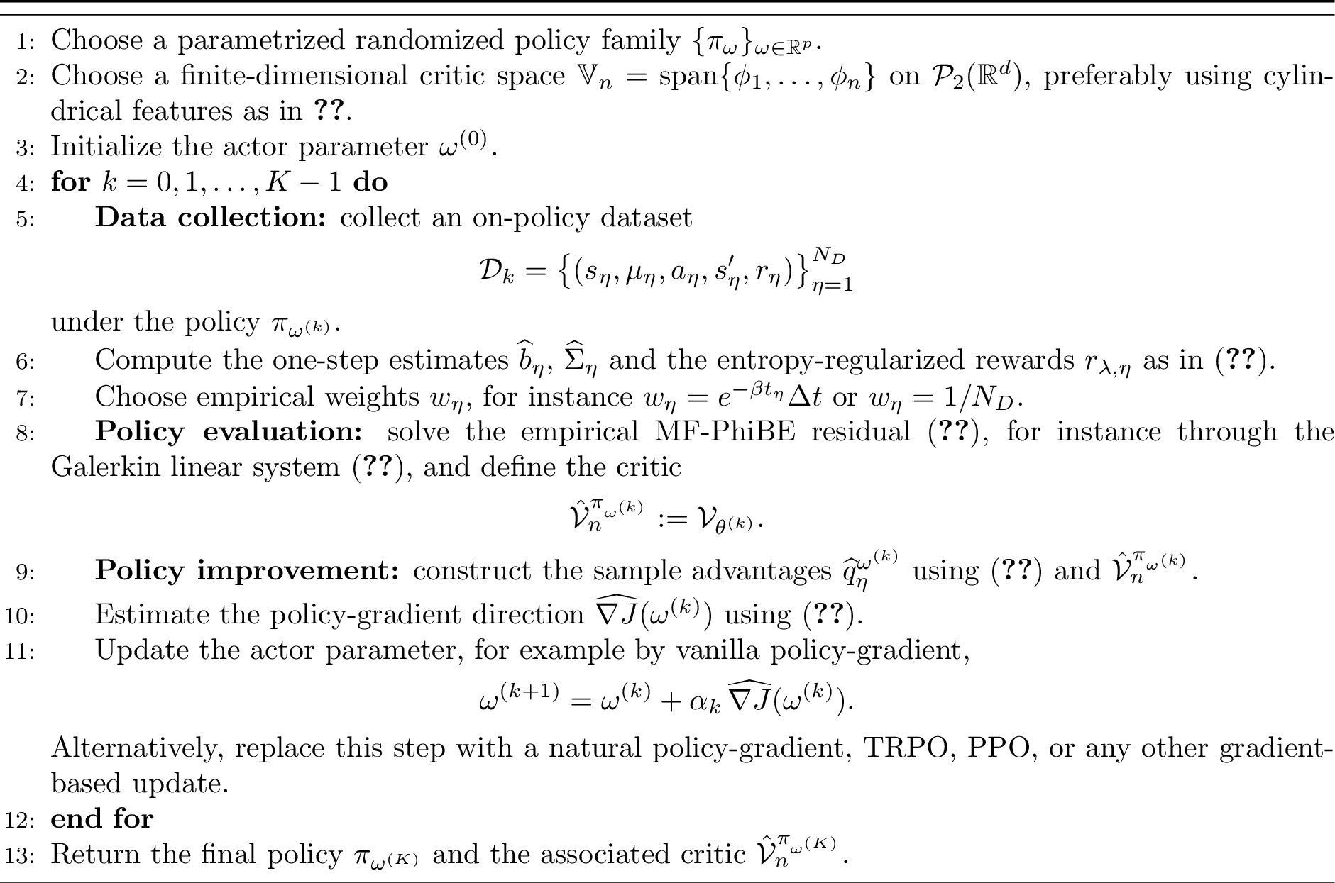
7 Numerical examples↩︎
7.1 Example 1: Model-free systemic risk↩︎
We first consider the systemic-risk specialization of the LQR McKean-Vlasov control problem studied in 5. This example admits an explicit Riccati characterization of the continuous-time optimal policy and therefore provides a benchmark to compare our algorithm.
7.1.1 Problem setup↩︎
We work in dimension \(d=m=1\) and impose the systemic-risk relation \(\bar A=-A\) in 13 . The controlled population dynamics are therefore \[d s_t = \bigl(A(s_t-\bar\mu_t)+B a_t\bigr)\,dt + \gamma\,dB_t, \qquad \bar\mu_t:=\int_{\mathbb{R}}x\,\mu_t(dx), \qquad \mu_t=\mathop{\mathrm{\text{Law}}}(s_t).\] The running reward is the quadratic reward introduced in 14 , and the entropy-regularized averaged reward is defined by 3 . The exact optimal policy is obtained from the Riccati system in 5. We use this explicit solution as a reference to illustrate the model-free actor-critic algorithm introduced in 6.
7.1.2 Policy parametrization, value approximation and gradient direction↩︎
Following the explicit LQR structure, we use the Gaussian policy class \[\begin{align} \label{eq:definition95paramtric95policy95ex1} \pi_\omega(\cdot\mid s,\mu) = \mathcal{N}\left( \omega_1(s-\bar\mu)+\omega_2\bar\mu,\, \frac{\lambda}{2}N^{-1} \right), \qquad \omega=(\omega_1,\omega_2)\in\mathbb{R}^2. \end{align}\tag{28}\] The critic is parametrized by the quadratic law-value ansatz \[\begin{align} \label{eq:value95anzatz95ex1} \mathcal{V}_\theta(\mu) = \theta_1+\theta_2\,\bar\mu^2+\theta_3\,\operatorname{Var}(\mu), \qquad \theta=(\theta_1,\theta_2,\theta_3)\in\mathbb{R}^3. \end{align}\tag{29}\] In this finite-dimensional setting, the Lions derivative of the critic is \(\partial_\mu \mathcal{V}_\theta(\mu)(s) = 2\theta_2\bar\mu + 2\theta_3(s-\bar\mu).\) As in the LQR-MF-PhiBE approximation considered in 5, we use the drift-only surrogate and set \(\widehat\Sigma=0\) in the empirical advantage. Thus, for a data point \((s_\eta,\mu_\eta,a_\eta,s'_\eta,r_\eta)\), with \(\bar\mu_\eta=\int x\,\mu_\eta(dx)\), the sample advantage used in the actor update is \[\begin{align} \label{eq:explicit95q95LQR} \widehat q_\eta = r_\eta - \lambda\log p_{\pi_\omega}(a_\eta\mid s_\eta,\mu_\eta) + \widehat b_\eta \left( 2\theta_2\bar\mu_\eta + 2\theta_3(s_\eta-\bar\mu_\eta) \right), \end{align}\tag{30}\] with \(\hat{b}\) defined in 20 . Since the policy variance is fixed, the score function is \[\begin{align} \label{eq:score95explicit95lqr} \nabla_\omega\log p_{\pi_\omega}(a_\eta\mid s_\eta,\mu_\eta) = \frac{a_\eta-\omega_1(s_\eta-\bar\mu_\eta)-\omega_2\bar\mu_\eta}{\lambda(2N)^{-1}} \begin{pmatrix} s_\eta-\bar\mu_\eta\\ \bar\mu_\eta \end{pmatrix}. \end{align}\tag{31}\] Hence the empirical policy-gradient direction used in the experiment is computed by substituting 30 and 31 into 26 , with either discounted weights \(w_\eta=e^{-\beta t_\eta}\Delta t\) or uniform weights \(w_\eta=1/N_D\).
7.1.3 Implementation and numerical results↩︎
Since the policy parametrization in 28 and the value-function ansatz 29 depend on the law only through \(\bar\mu_\eta\) and \(\operatorname{Var}(\mu_\eta)\), in this example we do not need a full empirical representation of \(\mu_\eta\). Hence, for a fixed policy \(\pi_\omega\), we assume that the available data set is \[\mathcal{D}_\omega = \left\{ \bigl( s_\ell^i,\bar\mu^i,\operatorname{Var}(\mu^i), a_\ell^i,r_\ell^i,(s_\ell^i)' \bigr) : i=1,\ldots,N_{\rm steps},\;\ell=1,\ldots,L \right\}.\] Here \(N_{\rm steps}\) is the number of observed one-step transitions along each trajectory, and \(L\) is the number of independent trajectories, obtained from independent samples of the initial law. We have \(s_\ell^i\sim\mu^i\), \(a_\ell^i\sim\pi_\omega(\cdot\mid s_\ell^i,\mu^i)\), \(r_\ell^i=r(s_\ell^i,\mu^i,a_\ell^i)\), and \((s_\ell^i)'\) denotes the state observed after one time step \(\Delta t\).
To reduce artificial sources of noise, the data are generated exactly from the LQR dynamics, thereby avoiding an additional numerical time-discretization error. More precisely, \((s_\ell^i)'\) is sampled from the explicit transition law 17 , while the moments of the law are propagated through the closed equations associated with the current policy: \(\dot{\bar\mu}_t=(A+\bar A+B\omega_2)\bar\mu_t\) and \(\frac{d}{dt}\operatorname{Var}(\mu_t)=2(A+B\omega_1)\operatorname{Var}(\mu_t)+\gamma^2\).
In the numerical experiment we use \(N_{\rm steps}=50\), \(L=200\), and \(\Delta t=0.05\). The numerical parameters are \[\begin{align} \label{eq:parameters95example1} A=-1,\quad \bar A=1,\quad B=1,\quad Q=1,\quad \bar Q=1,\quad N=0.5,\quad\beta=1,\quad \gamma=0.5,\quad \lambda=0.2. \end{align}\tag{32}\] The initial law is \(\mu=\mathcal{N}(1,1)\). The empirical estimators entering 30 , 31 and 26 are computed from \(\mathcal{D}_\omega\).
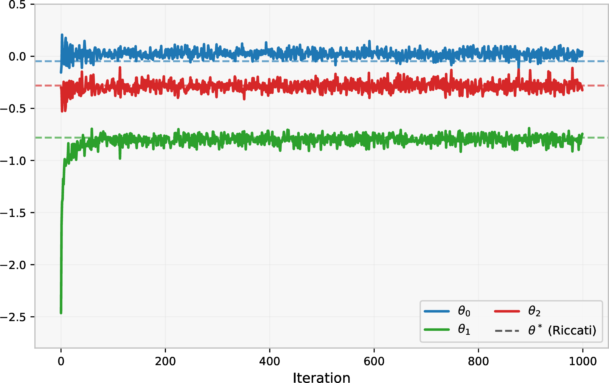
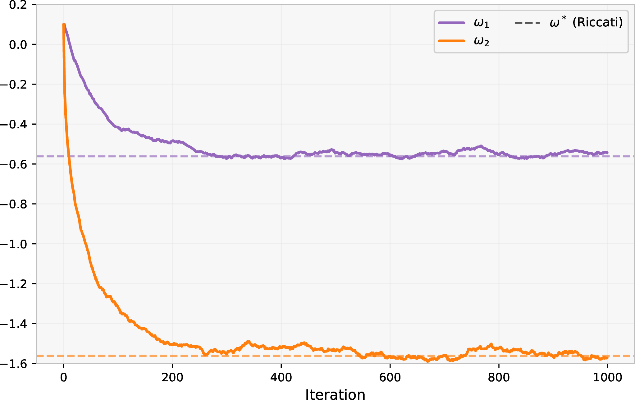
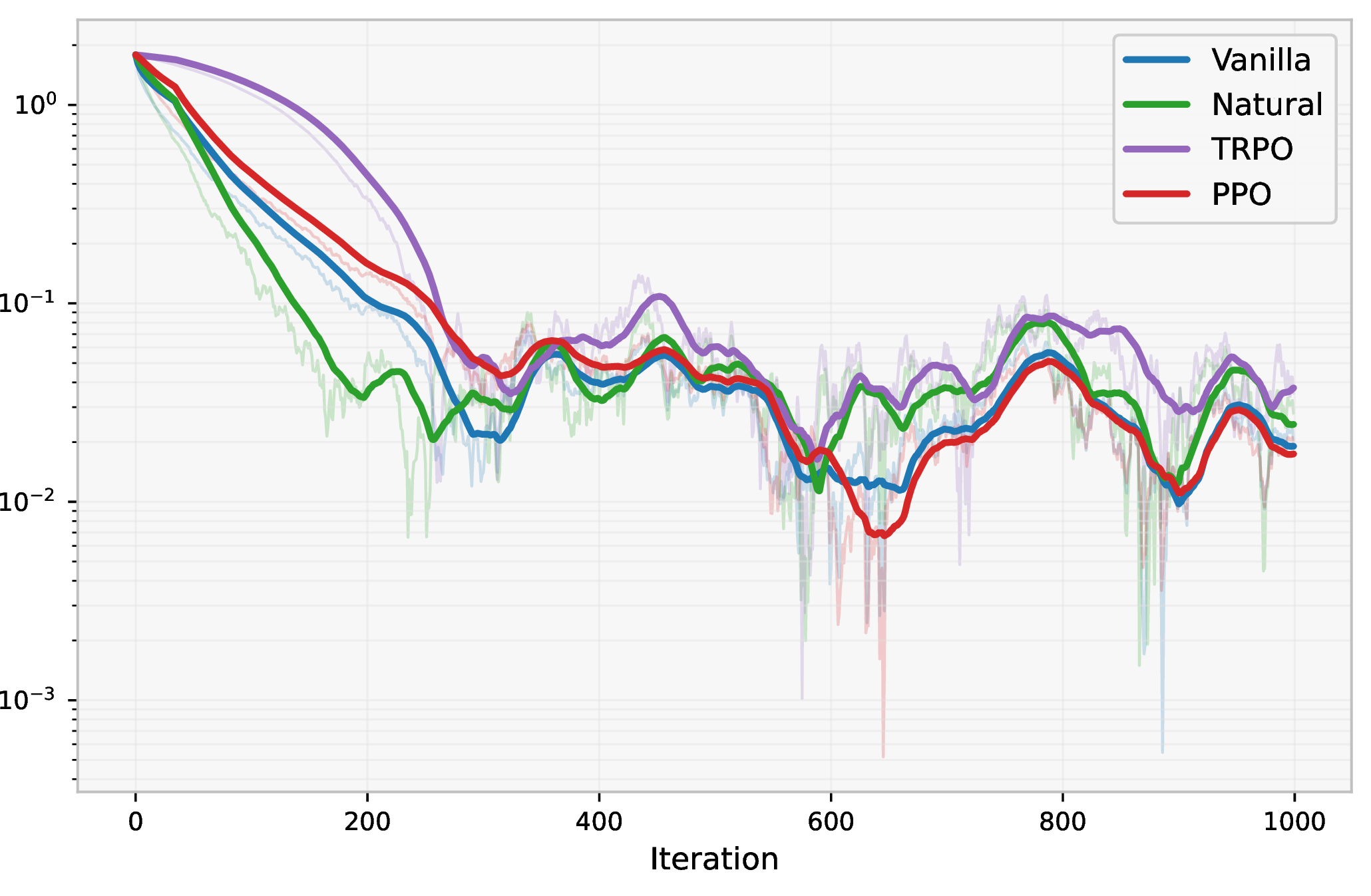
Figure 4: Model-free LQR-MF-PhiBE actor-critic convergence. Left: critic parameters obtained from the empirical MF-PhiBE evaluation, compared with the Riccati reference. Center: actor parameters produced by the vanilla policy-gradient update, compared with the optimal feedback parameters. Right: policy-parameter error for different update rules..
4 illustrates the behavior of the actor-critic scheme in the LQR benchmark when the discounted occupancy measure \(w_\eta=e^{-\beta t_\eta}\Delta t\) is used. The left panel shows that the empirical critic recovers the quadratic value structure predicted by the Riccati solution. The center panel shows that the actor parameters approach the optimal feedback coefficients. The right panel compares several update rules, namely vanilla gradient descent, natural gradient descent, TRPO, and PPO; see 6.2.1. This panel shows a consistent reduction of the policy-parameter error, with residual oscillations caused by the finite data set used at each update. Thus, the experiment confirms that the empirical MF-PhiBE critic provides a usable policy-gradient direction for recovering the continuous-time LQR feedback. Similarly, the left and center panels of 5 show analogous results for the undiscounted occupancy measure \(w_\eta=1/N_D\), where convergence is also observed.
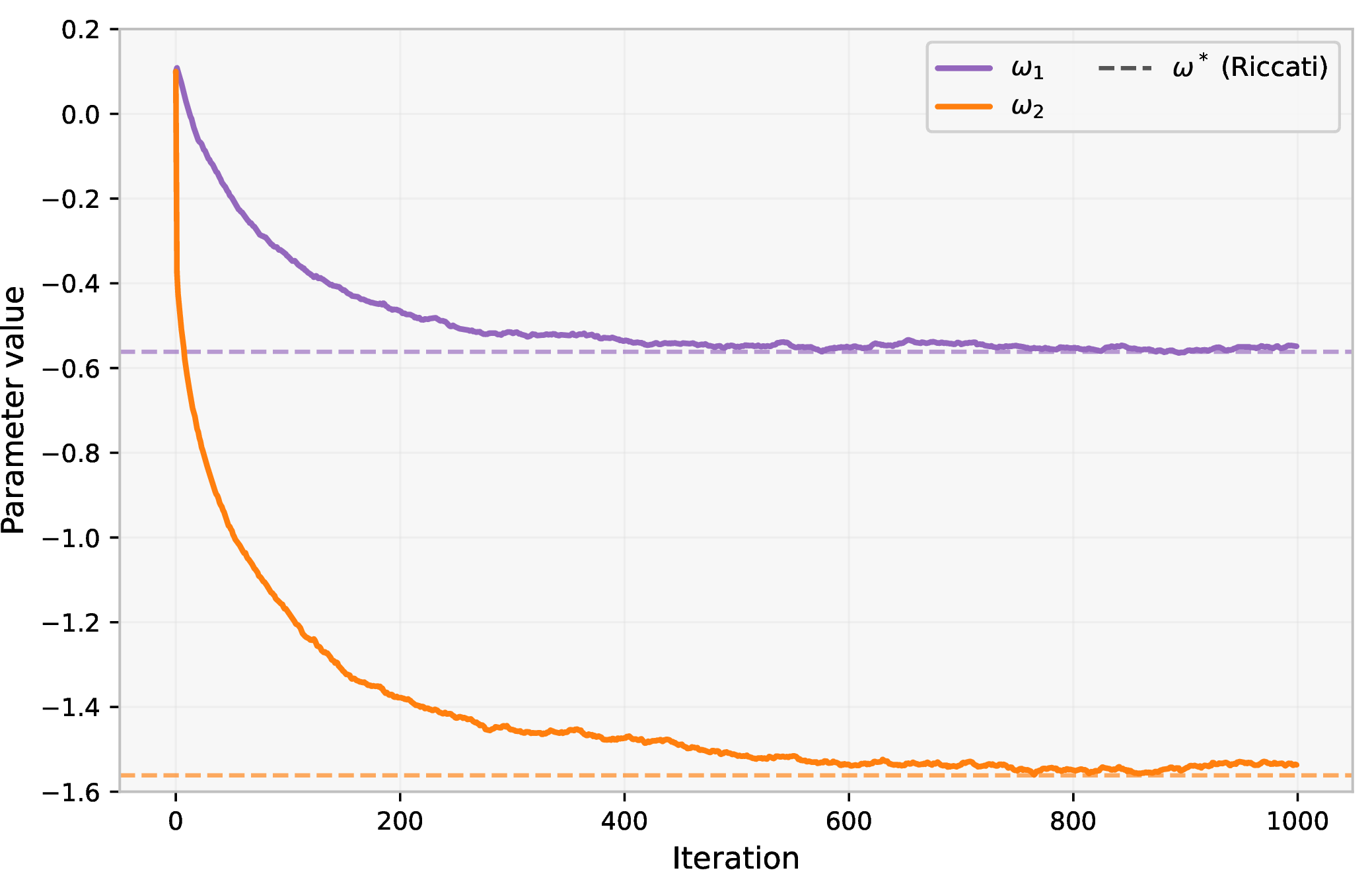
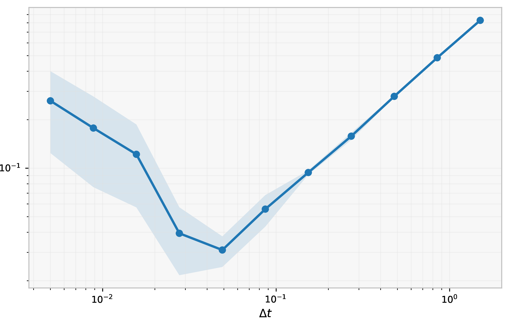
Figure 5: Undiscounted performance and sample-complexity effect. Left: critic parameters obtained from the empirical MF-PhiBE using the undiscounted occupancy measure. Center: actor parameters produced by the vanilla policy-gradient update using the undiscounted occupancy measure. Right: continuous-time value error as a function of the observation step \(\Delta t\), using a fixed data budget \(N_D=4800\)..
The right panel of 5 shows the effect of decreasing \(\Delta t\) while keeping the total number of observations fixed. For large and moderate values of \(\Delta t\), reducing the observation step improves the approximation, as expected from the consistency of the one-step MF-PhiBE estimator. However, once \(\Delta t\) becomes too small, the error starts increasing. In this regime the dominant error is no longer the finite-\(\Delta t\) approximation error, but the statistical error produced by the fixed data budget. Thus, the curve exhibits a threshold beyond which more accurate time resolution is not beneficial unless the number of samples is also increased.
7.1.4 Comparison with the time-discrete Bellman problem↩︎
The previous experiment evaluates the LQR-MF-PhiBE approximation of the continuous-time control problem. We now compare this construction with a different way of using observations at time step \(\Delta t\): instead of incorporating the one-step information into the continuous-time HJB structure, one may first discretize the controlled dynamics and then solve the resulting time-discrete Bellman problem.
Let \(\rho_{\Delta t}(\cdot\mid s,\mu,a)\) denote the one-step transition kernel induced by 17 . The corresponding discretized entropy-regularized objective is \[\mathcal{V}_{\Delta t}^{\pi}(\mu) := \mathbb{E}\left[ \sum_{i=0}^{\infty} e^{-\beta i\Delta t}\, \Delta t\, r_\lambda^\pi(\mu_i) \,\bigg|\, \mu_0=\mu \right],\] where the controlled Markov chain is defined by \[s_{i+1}\sim \rho_{\Delta t}(\cdot\mid s_i,\mu_i,a_i), \qquad a_i\sim\pi(\cdot\mid s_i,\mu_i), \qquad \mu_i=\mathop{\mathrm{\text{Law}}}(s_i).\]
The discrete-time problem still admits an explicit Gaussian optimizer. Set \(\delta:=e^{-\beta\Delta t}\) and \(B_{\Delta t}:=\Delta t\,\hat{B}\), where \(\hat{B}\) is the action coefficient in the one-step drift estimator 19 . Set \[A_{\Delta t}:=I+\Delta t\,\hat{A}, \qquad \widetilde{A}_{\Delta t}:=I+\Delta t(\hat{A}+\hat{\bar A}), \qquad B_{\Delta t}:=\Delta t\,\hat{B}, \qquad \delta:=e^{-\beta\Delta t}.\] Then, the optimal policy of the discretization problem is given by \[\pi_{\Delta t}^*(\cdot\mid s,\mu) = \mathcal{N}\left( \bar{\pi}_{\Delta t}^*(s,\mu), \Sigma_{\Delta t}^* \right), \qquad \Sigma_{\Delta t}^* = \frac{\lambda\Delta t}{2} \left( \Delta t\,N + \delta B_{\Delta t}^{\top}K_{\Delta t}B_{\Delta t} \right)^{-1},\] with \[\begin{align} \bar{\pi}_{\Delta t}^*(s,\mu) = &- \left[ \left( \Delta t\,N + \delta B_{\Delta t}^{\top}K_{\Delta t}B_{\Delta t} \right)^{-1} \delta B_{\Delta t}^{\top}K_{\Delta t}A_{\Delta t} \right](s-\bar\mu) \\ &- \left[ \left( \Delta t\,N + \delta B_{\Delta t}^{\top}\Lambda_{\Delta t}B_{\Delta t} \right)^{-1} \delta B_{\Delta t}^{\top}\Lambda_{\Delta t}\widetilde{A}_{\Delta t} \right]\bar\mu . \end{align}\] Here the matrices \(K_{\Delta t}\) and \(\Lambda_{\Delta t}\) are the stabilizing solutions of \[\begin{align} K_{\Delta t} &= \Delta t\,Q + \delta A_{\Delta t}^{\top} K_{\Delta t} A_{\Delta t} - \delta^2 A_{\Delta t}^{\top} K_{\Delta t}B_{\Delta t} \left( \Delta t\,N + \delta B_{\Delta t}^{\top}K_{\Delta t}B_{\Delta t} \right)^{-1} B_{\Delta t}^{\top}K_{\Delta t} A_{\Delta t}, \\ \Lambda_{\Delta t} &= \Delta t\,(Q+\bar Q) + \delta \widetilde{A}_{\Delta t}^{\top} \Lambda_{\Delta t} \widetilde{A}_{\Delta t} - \delta^2 \widetilde{A}_{\Delta t}^{\top} \Lambda_{\Delta t}B_{\Delta t} \left( \Delta t\,N + \delta B_{\Delta t}^{\top}\Lambda_{\Delta t}B_{\Delta t} \right)^{-1} B_{\Delta t}^{\top}\Lambda_{\Delta t} \widetilde{A}_{\Delta t}. \end{align}\] The optimal policy characterization is obtained by combining the time-discrete mean-field LQ framework of [40] with the entropy-regularized one-step Bellman minimization of [41]. The former motivates the discrete mean-field LQ structure, while the latter yields a Gaussian optimizer over randomized feedback policies, with covariance proportional to \(\lambda\Delta t\).
For fixed \(\Delta t>0\), neither the discrete optimizer \(\pi_{\Delta t}^*\) nor the LQR-MF-PhiBE optimizer \(\hat{\pi}^*\) is expected to coincide exactly with the continuous-time optimizer \(\pi^*\). The question is therefore which of the two finite-\(\Delta t\) approximations is closer to \(\pi^*\). To compare policies, for Gaussian feedback laws \[\pi_i(\cdot\mid s,\mu) = \mathcal{N}\left( -L_c^i(s-\bar\mu)-L_m^i\bar\mu, \Sigma_i \right), \qquad i=1,2,\] we use \[\begin{align} \label{eq:difinition95E952} \mathcal{E}_2(\pi_1,\pi_2) := \left( \|L_c^1-L_c^2\|^2 + \|L_m^1-L_m^2\|^2 + \|\Sigma_1^{1/2}-\Sigma_2^{1/2}\|_F^2 \right)^{1/2}. \end{align}\tag{33}\] In particular, for every compact set \(K\subset \mathbb{R}^d\times\mathbb{R}^d\), there exists \(C_K>0\) such that \[\begin{align} \label{eq:relation95W95295E952} \sup_{(s,\bar\mu)\in K} \mathcal{W}_2\bigl( \pi_1(\cdot\mid s,\mu), \pi_2(\cdot\mid s,\mu) \bigr) \le C_K\mathcal{E}_2(\pi_1,\pi_2). \end{align}\tag{34}\]

In 6, the first panel shows how the policy error depends on the discount factor for fixed values of \(\Delta t\). Throughout this experiment, we use the same parameters as in 32 . For the parameter values displayed in this experiment, the LQR-MF-PhiBE policy remains closer to \(\pi^*\) than the discrete-time optimizer over the plotted range of \(\beta\). The second panel confirms that both policy errors decrease as \(\Delta t\to0\), as expected from the consistency of both finite-\(\Delta t\) approximations. The third panel shows the same comparison at the level of the original continuous-time objective: the value gap decreases with \(\Delta t\), and the relative ordering of the two methods is consistent with the policy-error plots. Finally, the fourth panel evaluates the performance of the two optimal policies as observations become more frequent. More precisely, the LQR-MF-PhiBE and discrete-time policies are computed once with \(\Delta t=0.5\) and then applied to the continuous dynamics with observations taken every \(h\) units of time. The plot shows that, as observations become more frequent, the LQR-MF-PhiBE policy yields a smaller exact value error than the discrete-time policy. Moreover, as \(h\) decreases, the observed errors stabilize, which indicates that the remaining discrepancy is mainly due to the policy approximation itself rather than to the frequency at which the closed-loop system is observed.
Let \(\operatorname{Err}_{\mathrm{PhiBE}}:=\mathcal{E}(\pi^*,\hat{\pi}^*)\) and \(\operatorname{Err}_{\mathrm{disc}}:=\mathcal{E}(\pi^*,\pi_{\Delta t}^*)\). To identify the parameter regimes in which one approximation is more accurate than the other, 7 plots the logarithmic ratio \(\log(\operatorname{Err}_{\mathrm{PhiBE}}/\operatorname{Err}_{\mathrm{disc}})\). Negative values mean that LQR-MF-PhiBE has the smaller policy error, while positive values mean that the optimizer of the time-discrete Bellman problem is closer to \(\pi^*\). The black curve marks the zero level set, where both errors coincide. The heatmaps in 7 show that the relative accuracy depends on the parameter regime. In the displayed experiments, LQR-MF-PhiBE is more accurate in a large part of the parameter range, whereas direct discretization becomes more accurate only in the regime when \(A\) and \(B\) are small enough. This confirms that the time-discrete Bellman problem and LQR-MF-PhiBE define two different finite-\(\Delta t\) approximations of the same continuous-time optimizer.
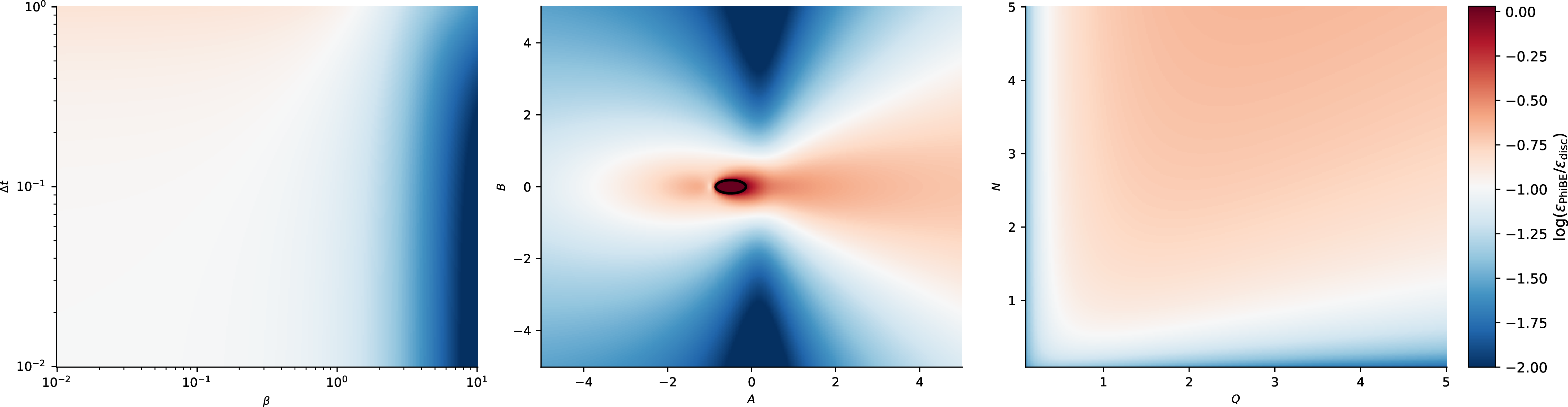
7.2 Example 2: Crowd aversion transport↩︎
We next test the model-free MF-PhiBE actor-critic method on a nonlinear two-dimensional McKean-Vlasov control problem. The objective is to transport the population toward a prescribed target location while penalizing concentration in regions of high crowd density. This experiment is formulated directly at the level of the population law.
7.2.1 Problem setup↩︎
The controlled population law \(\mu_t\) is generated by \[ds_t = a_t\,dt + \sigma\,dW_t, \qquad a_t \sim \pi_\omega(\cdot \mid s_t,\mu_t), \qquad \mu_t=\mathop{\mathrm{\text{Law}}}(s_t),\] where \(s_t\in\mathbb{R}^2\), \(a_t\in\mathbb{R}^2\), and \(\sigma>0\) is fixed. The running reward is \[r(s,\mu,a) = -\left( \frac{1}{2}\|a\|^2 + \frac{\kappa}{2}\|s-s_{\rm tar}\|^2 + \gamma (K_\eta * \mu)(s) + \frac{\rho}{2}\|s\|^2 \right).\] Here \(s_{\rm tar}\in\mathbb{R}^2\) is the target, \(\kappa>0\) controls target attraction, \(\gamma>0\) controls crowd aversion, and \(\rho\geq 0\) is a mild confinement parameter used for numerical stability. The crowd-density term is \[(K_\eta * \mu)(s) = \int_{\mathbb{R}^2} \exp\left(-\frac{\|s-y\|^2}{2\eta^2}\right)\mu(dy),\] where \(\eta>0\) is the kernel bandwidth. We consider the entropy-regularized reward introduced in 3 . The law-level objective is the discounted infinite-horizon value \(\mathcal{V}^{\pi_\omega}\) in 2 .
Remark 29 (Interpretation of the reward). The four terms in the running cost correspond, respectively, to control effort, target attraction, crowd aversion, and mild confinement. Since the controlled equation is linear and the control acts directly as a velocity field, the learned policy is expected to transport the population toward \(s_{\rm tar}\) while avoiding excessive concentration of mass, with the confinement term preventing particles from drifting too far from the target region.
7.2.2 Policy and value approximation↩︎
Motivated by the crowd-density term in the reward, we use Gaussian kernel features of the population law. Let \(c_1,\ldots,c_{M_\mu}\in\mathbb{R}^2\) be grid centers and let \(h>0\) be a bandwidth. We define \[u_j(\mu) = \int_{\mathbb{R}^2} \exp\left(-\frac{\|y-c_j\|^2}{2h^2}\right)\mu(dy), \qquad j=1,\ldots,M_\mu.\] We use a Gaussian policy with fixed exploration covariance, \[\pi_\omega(\cdot\mid s,\mu) = \mathcal{N}\left(m_\omega(s,\mu),\sigma_a^2 I_2\right), \qquad m_\omega(s,\mu)=W f(s,\mu), \qquad \omega\equiv W\in\mathbb{R}^{2\times d_f},\] where the feature vector \(f(s,\mu)\) is given by \[f(s,\mu) = \Bigl( 1,\, s,\, s-s_{\rm tar},\, \|s-s_{\rm tar}\|^2,\, u_1(\mu),\ldots,u_{M_\mu}(\mu) \Bigr)^\top .\] Thus, in this two-dimensional example, the number of actor features is \(d_f=6+M_\mu\). For the critic, we use the cylindrical approximation \[\mathcal{V}_\theta(\mu)=\theta^\top \Phi(u(\mu)), \qquad u(\mu)=(u_1(\mu),\ldots,u_{M_\mu}(\mu)).\] The feature map \(\Phi\) contains the constant, the linear terms in \(u\), and all quadratic products: \[\Phi(u) = \Bigl( 1,\, u_1,\ldots,u_{M_\mu},\, \{u_i u_j\}_{1\leq i\leq j\leq M_\mu} \Bigr)^\top .\] Thus, the critic has \(1+M_\mu+M_\mu(M_\mu+1)/2\) features. The Lions derivatives \(\partial_\mu \mathcal{V}_\theta(\mu)(x)\) and \(D_x\partial_\mu \mathcal{V}_\theta(\mu)(x)\) are computed analytically from this cylindrical representation.
7.2.3 Empirical MF-PhiBE critic and policy improvement↩︎
At policy iteration \(k\), we simulate \(L\) independent empirical population trajectories, each consisting of \(M\) particles and \(N_{\rm steps}\) time steps. For trajectory \(\ell\) and time index \(i\), the empirical law is \[\widehat\mu_\ell^i = \frac{1}{M}\sum_{j=1}^M \delta_{s_{\ell,j}^i}.\] Given \(\widehat\mu^i\), we sample \(a_j^i\sim \pi_{\omega_k}(\cdot\mid s_j^i,\widehat\mu^i)\), for \(j=1,\ldots,M\). Since the controlled equation is linear with constant diffusion, the particles are evolved exactly using the one-step transition law 17 , with the sampled action held constant over the observation interval. This introduces no additional numerical time-discretization error in the data generation. The data available at policy iteration \(k\) are \[\mathcal{D}_{\omega_k} = \left\{ \bigl( s_{\ell,j}^i,\widehat\mu_\ell^i, a_{\ell,j}^i,r_{\ell,j}^i,(s_{\ell,j}^i)' \bigr) : i=1,\ldots,N_{\rm steps},\;\ell=1,\ldots,L,\;j=1,\ldots,M \right\}.\] The critic parameter \(\theta\) is obtained from the Galerkin problem 24 using the one-step coefficient estimators \(\widehat b_n^i\) and \(\widehat\Sigma_n^i\) in 20 . We use either discounted weights \(w_n=e^{-\beta t_n}\Delta t/L\) or undiscounted finite-horizon weights \(w_n=\Delta t/L\).
Once the MF-PhiBE critic has been computed, we evaluate the sample infinitesimal advantage \(\widehat q_n^i\) in 27 and compute the empirical policy-gradient direction \[\widehat{\nabla J}(\omega_k) = \sum_n w_n\frac{1}{M}\sum_{i=1}^M (\widehat q_n^i-\overline{q}) \nabla_\omega\log p_{\pi_{\omega_k}}(a_n^i\mid s_n^i,\widehat\mu_n),\] with score term given by the explicit expression \[\nabla_W\log p_{\pi_{\omega_k}}(a\mid s,\mu) = \frac{1}{\sigma_a^2} \left(a-m_{\omega_k}(s,\mu)\right)f(s,\mu)^\top.\]
7.2.4 Implementation and numerical results↩︎
For the numerical simulations, we use \[\sigma=0.2, \qquad \beta=0.1, \qquad \kappa=1000, \qquad \gamma=10, \qquad \eta=0.8, \qquad \rho=0.1, \qquad \lambda=2.\] The initial law is concentrated near \(x_0=(-2,0)^\top\), with standard deviation \(0.02\), and the target is \(x_{\rm tar}=(2,0)^\top\). We train with \(\Delta t=0.1\), \(T=4.5\), \(L=50\) empirical trajectories per policy update, \(N_{\rm steps}=45\) time-steps, \(M=40\) particles per empirical law, and \(M_\mu=9\) law features, corresponding to a \(3\times 3\) grid of centers \(c_1,\ldots,c_9\). The policy uses fixed covariance \(\sigma_a^2 I_2\), with \(\sigma_a=0.25\).


Figure 8: Crowd aversion experiment. Left: training curves for several actor updates. Right: simulated population trajectories under the learned policy..
8 illustrates the behavior of the model-free MF-PhiBE actor-critic scheme in the crowd aversion problem. The left panel compares the training curves obtained with vanilla policy gradient, natural policy gradient, TRPO, and PPO. All methods improve the value during training, with different transient behavior depending on the update rule. The right panel shows representative trajectories under the learned policy. The population is transported from the initial region near \((-2,0)\) toward the target near \((2,0)\), while the empirical distribution spreads around the target due to the diffusion, the exploration covariance, and the crowd-aversion penalty, consistently with the interpretation of the reward given in 29.
8 Acknowledgements↩︎
E. Bayraktar is supported in part by NSF grants DMS-2507940 and 2406232, and in part by the Susan M. Smith Professorship. Y. Zhu and M. Hernandez are supported in part by NSF grant No. 2529107.
9 Proof of the main results↩︎
9.1 Proofs for Section 3.1↩︎
Proof of 4. Let \(V^\pi(s,\mu)\) be the value function of the coupled representative-population problem in [37], associated with the same fixed policy \(\pi\). By [37] Theorem 3.3, under 2, the coupled value function satisfies \(V^\pi\in \mathcal{C}^{2,2}_{\mathrm{poly}} (\mathbb{R}^d\times\mathcal{P}_2(\mathbb{R}^d))\) (the space of functions with polynomial growth that are twice differentiable in \(s\) and \(\mu\); see [37]) and solves \[\label{eq:coupled-HJB-used-mkv} (\mathscr L_{b,\Sigma}^{\pi}-\beta)V^\pi(s,\mu) +\ell_\lambda^\pi(s,\mu)=0,\tag{35}\] where \(\mathscr L_{b,\Sigma}^{\pi}\) being the generator on \(\mathbb{R}^d\times\mathcal{P}_2(\mathbb{R}^d)\) defined as \[\label{eq:L-pi} \begin{align} (\mathscr{L}_{b,\Sigma}^{\pi}F)(s,\mu) &:= b^{\pi}(s,\mu)\cdot\nabla_s F(s,\mu) + \tfrac{1}{2}\,\Sigma^{\pi}(s,\mu) : \nabla^2_{ss} F(s,\mu)\\ &\quad + \int_{\mathbb{R}^d} \Bigl[ b^{\pi}(\xi,\mu)\cdot \partial_{\mu}F(s,\mu)(\xi) + \tfrac{1}{2}\,\Sigma^{\pi}(\xi,\mu) : D_\xi\partial_{\mu}F(s,\mu)(\xi) \Bigr]\,\mu(d\xi), \end{align}\tag{36}\] On the other hand, since the initial condition in 5 satisfies \(s_0\sim\mu\), conditioning on \(s_0=s\), using Fubini’s theorem, we have \[\begin{align} \label{eq:mkv-value-as-integrated-coupled-value} \begin{aligned} \mathcal{V}^\pi(\mu) &= \mathbb{E}\left[ \int_0^\infty e^{-\beta t} \ell_\lambda^\pi(s_t,\mu_t)\,dt \,\bigg|\,\mu_0=\mu \right] = \int_{\mathbb{R}^d} \mathbb{E}\left[ \int_0^\infty e^{-\beta t} \ell_\lambda^\pi(s_t,\mu_t)\,dt \,\bigg|\,s_0=s,\;\mu_0=\mu \right]\mu(ds) \\ &= \int_{\mathbb{R}^d}V^\pi(s,\mu)\,\mu(ds). \end{aligned} \end{align}\tag{37}\] Since \(V^\pi\in\mathcal{C}^{2,2}_{\mathrm{poly}}\), applying the Lions derivative formula for maps of the form \(\mu\mapsto\int_{\mathbb{R}^d} V^\pi(s,\mu)\,\mu(ds)\) [7] yields \[\label{eq:mkv-value-lions-derivative} \partial_\mu\mathcal{V}^\pi(\mu)(x) = \nabla_sV^\pi(x,\mu) + \int_{\mathbb{R}^d} \partial_\mu V^\pi(s,\mu)(x)\,\mu(ds),\tag{38}\] and \[\label{eq:mkv-value-lions-second-derivative} D_x\partial_\mu\mathcal{V}^\pi(\mu)(x) = \nabla^2_{ss}V^\pi(x,\mu) + \int_{\mathbb{R}^d} D_x\partial_\mu V^\pi(s,\mu)(x)\,\mu(ds).\tag{39}\] The polynomial bounds in the definition of \(\mathcal{C}^2_{\mathrm{poly}}(\mathcal{P}_2(\mathbb{R}^d))\) follow directly from the corresponding bounds for \(V^\pi\). Hence \(\mathcal{V}^\pi\in \mathcal{C}^2_{\mathrm{poly}}(\mathcal{P}_2(\mathbb{R}^d))\). Using 38 and 39 , we compute \[\begin{align} (\mathcal{L}_{b,\Sigma}^{\pi}\mathcal{V}^\pi)(\mu) &= \int_{\mathbb{R}^d} \left[ b^\pi(x,\mu)\cdot\nabla_sV^\pi(x,\mu) + \frac{1}{2}\Sigma^\pi(x,\mu):\nabla^2_{ss}V^\pi(x,\mu) \right]\mu(dx) \\ &\quad+ \int_{\mathbb{R}^d}\int_{\mathbb{R}^d} \left[ b^\pi(x,\mu)\cdot\partial_\mu V^\pi(s,\mu)(x) + \frac{1}{2}\Sigma^\pi(x,\mu): D_x\partial_\mu V^\pi(s,\mu)(x) \right]\mu(dx)\mu(ds) \\ &= \int_{\mathbb{R}^d} (\mathscr L_{b,\Sigma}^{\pi}V^\pi)(s,\mu)\,\mu(ds). \end{align}\] Integrating 35 with respect to \(\mu(ds)\) and using 37 gives \[(\mathcal{L}_{b,\Sigma}^{\pi}\mathcal{V}^\pi)(\mu) - \beta\mathcal{V}^\pi(\mu) + r_\lambda^\pi(\mu) = 0.\] Thus \(\mathcal{V}^\pi\) solves ?? .
We now prove uniqueness. Let \(U\in\mathcal{C}^2_{\mathrm{poly}}(\mathcal{P}_2(\mathbb{R}^d))\) be another classical solution of ?? . Applying the Itô-Lions formula to \(e^{-\beta t}U(\mu_t)\) gives \[\frac{d}{dt} \left(e^{-\beta t}U(\mu_t)\right) = e^{-\beta t} \left[ (\mathcal{L}_{b,\Sigma}^{\pi}U)(\mu_t) - \beta U(\mu_t) \right] = -e^{-\beta t}r_\lambda^\pi(\mu_t).\] Therefore, for every \(T>0\), \[U(\mu) = e^{-\beta T}U(\mu_T) + \int_0^T e^{-\beta t}r_\lambda^\pi(\mu_t)\,dt.\] By the polynomial growth of \(U\), there exists \(C_U>0\) such that \[|U(\nu)|\le C_U\bigl(1+m_2(\nu)\bigr), \qquad \nu\in\mathcal{P}_2(\mathbb{R}^d).\] Moreover, by [37], there exists \(C>0\) such that \[m_2(\mu_T)\le C e^{\beta_0(2)T}\bigl(1+m_2(\mu)\bigr), \qquad T\ge0.\] Since \(\beta>\bar\beta_\pi\) and, by [37], \(\bar\beta_\pi\ge \beta_0(2)\), we obtain \[e^{-\beta T}|U(\mu_T)| \le C e^{-\beta T} + C e^{-(\beta-\beta_0(2))T}\bigl(1+m_2(\mu)\bigr) \longrightarrow 0, \qquad T\to\infty.\] Hence \[U(\mu) = \int_0^\infty e^{-\beta t}r_\lambda^\pi(\mu_t)\,dt = \mathcal{V}^\pi(\mu).\] It remains to prove ?? . In [37], the finite-horizon derivatives of the coupled value functions are represented through the variational flows. The estimates [37] therein imply, after integration against \(e^{-\beta t}\), that \[\begin{align} |\nabla_sV^\pi(s,\nu)| + |\partial_\mu V^\pi(s,\nu)(x)| &\le \frac{C_\pi}{\beta-\bar\beta_\pi} \bigl(1+|s|+|x|+m_2(\nu)\bigr), \\ \|\nabla^2_{ss}V^\pi(s,\nu)\| + \|D_x\partial_\mu V^\pi(s,\nu)(x)\| &\le \frac{C_\pi}{\beta-\bar\beta_\pi} \bigl(1+m_2(\nu)\bigr). \end{align}\] The passage from the finite-horizon bounds to the infinite-horizon bounds follows from the locally uniform convergence of the derivatives proved in [37] Step 4 of the proof of Theorem 3.3.
Combining these estimates with 38 gives \[\begin{align} |\partial_\mu\mathcal{V}^\pi(\nu)(x)| &\le |\nabla_sV^\pi(x,\nu)| + \int_{\mathbb{R}^d} |\partial_\mu V^\pi(s,\nu)(x)|\,\nu(ds)\le \frac{C_\pi}{\beta-\bar\beta_\pi} \bigl(1+|x|^2+m_2(\nu)\bigr). \end{align}\] Similarly, using 39 , \[\begin{align} \|D_x\partial_\mu\mathcal{V}^\pi(\nu)(x)\| &\le \|\nabla^2_{ss}V^\pi(x,\nu)\| + \int_{\mathbb{R}^d} \|D_x\partial_\mu V^\pi(s,\nu)(x)\|\,\nu(ds) \le \frac{C_\pi}{\beta-\bar\beta_\pi} \bigl(1+|x|^2+m_2(\nu)\bigr). \end{align}\] This proves ?? . ◻
Proof of 8. Let \(V^{\pi^\varepsilon}\) denote the value function of the coupled state-law problem studied in [37]. Set \[J(\varepsilon) := \int_{\mathbb{R}^d} V^{\pi^\varepsilon}(s,\mu)\,\mu(ds).\] By 37 , \(J(\varepsilon)=\mathcal{V}^{\pi^\varepsilon}(\mu)=\mathcal{J}(\varepsilon)\). It is therefore enough to compute the derivative of \(J\) at \(\varepsilon=0\).
We apply [37] with initial population law \(\mu\) and initial representative law also equal to \(\mu_0=\mu\). Denote by \(\widehat\rho^\pi\) the corresponding discounted occupancy measure of the coupled state-law process. Then \(J\) is differentiable at \(\varepsilon=0\), and \[\begin{align} \frac{d}{d\varepsilon}J(\varepsilon)\bigg|_{\varepsilon=0} &=\frac{1}{\beta} \mathbb{E}_{(s,\eta)\sim\widehat\rho^\pi}\!\left[ \int_{\mathcal{A}} q_{\mathrm{rep}}^\pi(s,\eta,a)\, \varphi(da\mid s,\eta) + \int_{\mathbb{R}^d}\!\int_{\mathcal{A}} q_{\mathrm{pop}}^\pi(s,\eta,\xi,a)\, \varphi(da\mid \xi,\eta)\,\eta(d\xi) \right], \end{align}\] where, according to [37], \[\begin{align} q_{\mathrm{rep}}^\pi(s,\eta,a) &= r(s,\eta,a)-\lambda\log p_\pi(a\mid s,\eta) +b(s,\eta,a)\cdot\nabla_s V^\pi(s,\eta) \\ &\qquad\qquad\qquad+\frac{1}{2}\,\Sigma(s,\eta,a):D^2_{ss}V^\pi(s,\eta)-\beta V^\pi(s,\eta), \\ q_{\mathrm{pop}}^\pi(s,\eta,\xi,a) &= b(\xi,\eta,a)\cdot\partial_\mu V^\pi(s,\eta)(\xi) +\frac{1}{2}\,\Sigma(\xi,\eta,a):D_\xi\partial_\mu V^\pi(s,\eta)(\xi). \end{align}\]
Since the initial representative law is \(\mu\), the representative component in the coupled state-law system has law \(\mu_t^\pi\) at time \(t\). Hence, for every measurable \(F\) for which the following quantities are well defined, \[\begin{align} \label{eq:rho-transfer-mkv} \mathbb{E}_{(s,\eta)\sim\widehat\rho^\pi}[F(\eta,s)] = \int_0^\infty e^{-\beta t} \int_{\mathbb{R}^d} F(\mu_t^\pi,\xi)\,\mu_t^\pi(d\xi)\,dt = \mathbb{E}_{(\eta,\xi)\sim\rho^\pi}[F(\eta,\xi)]. \end{align}\tag{40}\] Applying this identity with \[F(\eta,\xi) := \int_{\mathcal{A}} \left[ q_{\mathrm{rep}}^\pi(\xi,\eta,a) + \int_{\mathbb{R}^d} q_{\mathrm{pop}}^\pi(s,\eta,\xi,a)\,\eta(ds) \right] \varphi(da\mid \xi,\eta),\] we obtain \[\begin{align} \label{eq:derivative95j95almost95finished} \begin{aligned} \frac{d}{d\varepsilon}\mathcal{J}(\varepsilon)\bigg|_{\varepsilon=0} &=\frac{1}{\beta} \mathbb{E}_{(\eta,\xi)\sim\rho^\pi}\!\left[ \int_{\mathcal{A}} \left[ q_{\mathrm{rep}}^\pi(\xi,\eta,a) + \int_{\mathbb{R}^d} q_{\mathrm{pop}}^\pi(s,\eta,\xi,a)\,\eta(ds) \right] \varphi(da\mid \xi,\eta) \right]. \end{aligned} \end{align}\tag{41}\] It remains to identify the term in brackets. By 38 , 39 , and [37], the representative and population kernels satisfy \[\begin{align} \label{eq:realtion95q95paper95195neq95q} q_{\mathrm{rep}}^\pi(\xi,\eta,a) + \int_{\mathbb{R}^d} q_{\mathrm{pop}}^\pi(s,\eta,\xi,a)\,\eta(ds) = q^\pi(\eta,\xi,a), \end{align}\tag{42}\] where \(q^\pi\) is the McKean-Vlasov advantage function defined in ?? . Substituting 42 into 41 gives ?? . ◻
Proof of 13. Fix \(\omega\in\mathbb{R}^p\) and set \(\pi:=\pi_\omega\). Define \(J(\omega):=\int_{\mathbb{R}^d}V^{\pi_\omega}(s,\mu)\,\mu(ds).\) As in the proof of 8, one has \(J(\omega)=\mathcal{V}^{\pi_\omega}(\mu)=\mathcal{J}(\omega)\), so it is enough to compute the gradient of \(J\).
By the parametric policy gradient theorem for \(J\) in the first paper, \(J\) is differentiable at \(\omega\) and \[\begin{align} \nabla_\omega J(\omega) &= \frac{1}{\beta}\mathbb{E}_{(s,\eta)\sim\widehat\rho^\pi}\!\left[ \int_{\mathcal{A}} q_{\mathrm{rep}}^\pi(s,\eta,a)\, \nabla_\omega\log p_\pi(a\mid s,\eta)\, \pi(da\mid s,\eta) \right]\\ &\qquad+ \frac{1}{\beta}\mathbb{E}_{(s,\eta)\sim\widehat\rho^\pi}\!\left[ \int_{\mathbb{R}^d}\!\int_{\mathcal{A}} q_{\mathrm{pop}}^\pi(s,\eta,\xi,a)\, \nabla_\omega\log p_\pi(a\mid \xi,\eta)\, \pi(da\mid \xi,\eta)\, \eta(d\xi) \right]. \end{align}\] Now repeat verbatim the reduction carried out in the proof of 8: use the transfer identity 40 to pass from \(\widehat\rho^\pi\) to \(\rho^\pi\). Then use the reduced expression 41 and the relation between the representative and population kernels with the single advantage function introduced in 42 to conclude ?? . The equivalent expectation form with \(a\sim\pi(\cdot\mid\xi,\eta)\) follows immediately from the definition of conditional expectation. ◻
9.2 Proofs for Section 4↩︎
Definition 7. We use the following pointwise notation. If \(f=f(s,\mu)\) is \(\mathcal{C}^{2,2}\) in \((s,\mu)\), then \[\label{eq:evaluation-seminorm} \begin{align} \left\vert\kern-0.25ex\left\vert\kern-0.25ex\left\vert f(s,\mu) \right\vert\kern-0.25ex\right\vert\kern-0.25ex\right\vert_{\xi} := &\,\|f(s,\mu)\| +\|\nabla_s f(s,\mu)\| +\|D_{ss}^2 f(s,\mu)\| + |\partial_\mu f(s,\mu)(\xi)| + \|D_\xi\partial_\mu f(s,\mu)(\xi)\|. \end{align}\qquad{(16)}\] The derivatives in ?? are always taken with respect to \((s,\mu)\). Any additional variables, such as \(a\) or \(z\), are treated as fixed parameters.
Lemma 1 (Local expansion for the frozen-action estimators). Assume 16. Fix \(a\in\mathcal{A}\) and \((s,\mu)\in\mathbb{R}^d\times\mathcal{P}_2(\mathbb{R}^d)\). Let \((\mu_t)_{t\in[0,\Delta t]}\) be the law flow associated with the frozen-action version of 5 , initialized at \(\mu\), that is, with \(b^\pi\) and \(\sigma^\pi\) replaced by \(b(\cdot,\cdot,a)\) and \(\sigma(\cdot,\cdot,a)\). Given this flow, let \((s_t)_{t\in[0,\Delta t]}\) solve \[ds_t = b(s_t,\mu_t,a)\,dt + \sigma(s_t,\mu_t,a)\,dB_t, \qquad s_0=s.\] For \(F\in\mathcal{C}^{2,2}_{\mathrm{poly}} (\mathbb{R}^d\times\mathcal{P}_2(\mathbb{R}^d))\), define \[\label{eq:frozen-action-generator-mkv} \begin{align} (\mathscr L_{b,\Sigma}^aF)(x,\nu) &:= b(x,\nu,a)\cdot\nabla_xF(x,\nu) +\frac{1}{2}\,\Sigma(x,\nu,a):D_{xx}^2F(x,\nu) \\ &\quad+ \int_{\mathbb{R}^d} \Bigl[ b(\eta,\nu,a)\cdot\partial_\nu F(x,\nu)(\eta) + \frac{1}{2}\,\Sigma(\eta,\nu,a):D_\eta\partial_\nu F(x,\nu)(\eta) \Bigr]\nu(d\eta), \end{align}\qquad{(17)}\] where \(\Sigma(x,\nu,a):=\sigma(x,\nu,a)\sigma(x,\nu,a)^\top\). Assume that \(\mathscr L_{b,\Sigma}^aF\in \mathcal{C}^{2,2}_{\mathrm{poly}}(\mathbb{R}^d\times\mathcal{P}_2(\mathbb{R}^d))\) and \[\sup_{\tau\in[0,\Delta t]} \mathbb{E}\!\left[ |(\mathscr L_{b,\Sigma}^a)^2F(s_\tau,\mu_\tau)| \right]<\infty .\] Then \[\label{eq:local-expansion-general-mkv} \frac{\mathbb{E}[F(s_{\Delta t},\mu_{\Delta t})]-F(s,\mu)}{\Delta t} = (\mathscr L_{b,\Sigma}^aF)(s,\mu) + R_F^{a,\Delta t}(s,\mu),\qquad{(18)}\] where \[\label{eq:local-expansion-remainder-mkv} |R_F^{a,\Delta t}(s,\mu)| \le \frac{\Delta t}{2} \sup_{\tau\in[0,\Delta t]} \mathbb{E}\!\left[ |(\mathscr L_{b,\Sigma}^a)^2F(s_\tau,\mu_\tau)| \right].\qquad{(19)}\] Moreover, for \(F_k(x,\nu):=x_k\) and \(G_{ij}^s(x,\nu):=(x_i-s_i)(x_j-s_j)\), one has \[\label{eq:Fk-identities-mkv} \frac{\mathbb{E}[F_k(s_{\Delta t},\mu_{\Delta t})]-F_k(s,\mu)}{\Delta t} = \hat{b}_k(s,\mu,a), \qquad (\mathscr L_{b,\Sigma}^aF_k)(s,\mu)=b_k(s,\mu,a),\qquad{(20)}\] and \[\label{eq:Gij-identities-mkv} \frac{\mathbb{E}[G_{ij}^s(s_{\Delta t},\mu_{\Delta t})]-G_{ij}^s(s,\mu)}{\Delta t} = \hat{\Sigma}_{ij}(s,\mu,a), \qquad (\mathscr L_{b,\Sigma}^aG_{ij}^s)(s,\mu)=\Sigma_{ij}(s,\mu,a).\qquad{(21)}\] In particular, whenever the remainders in ?? are finite for \(F_k\) and \(G_{ij}^s\), \[\hat{b}_k(s,\mu,a)-b_k(s,\mu,a) = R_{F_k}^{a,\Delta t}(s,\mu), \qquad \hat{\Sigma}_{ij}(s,\mu,a)-\Sigma_{ij}(s,\mu,a) = R_{G_{ij}^s}^{a,\Delta t}(s,\mu).\]
Proof. Since \((\mu_t)_{t\in[0,\Delta t]}\) is deterministic, the Itô-Lions formula applied to \(F(s_t,\mu_t)\) gives \[F(s_t,\mu_t) = F(s,\mu) + \int_0^t (\mathscr L_{b,\Sigma}^aF)(s_\tau,\mu_\tau)\,d\tau + M_t^F,\] with \[M_t^F = \int_0^t \nabla_xF(s_\tau,\mu_\tau) \sigma(s_\tau,\mu_\tau,a)\,dB_\tau .\] The polynomial growth of \(\nabla_xF\), the boundedness of the coefficients in 16, and the moment estimates for the frozen-action dynamics imply that \(M^F\) is a square-integrable martingale. Hence \[\mathbb{E}[F(s_t,\mu_t)]-F(s,\mu) = \int_0^t \mathbb{E}[ (\mathscr L_{b,\Sigma}^aF)(s_\tau,\mu_\tau) ]\,d\tau .\] Applying the same argument to \(\mathscr L_{b,\Sigma}^aF\) yields, for \(\tau\in[0,\Delta t]\), \[\mathbb{E}[ (\mathscr L_{b,\Sigma}^aF)(s_\tau,\mu_\tau) ] = (\mathscr L_{b,\Sigma}^aF)(s,\mu) + \int_0^\tau \mathbb{E}[ (\mathscr L_{b,\Sigma}^a)^2F(s_u,\mu_u) ]\,du .\] Combining the two identities gives \[\mathbb{E}[F(s_t,\mu_t)]-F(s,\mu) = t(\mathscr L_{b,\Sigma}^aF)(s,\mu) + \int_0^t\int_0^\tau \mathbb{E}[ (\mathscr L_{b,\Sigma}^a)^2F(s_u,\mu_u) ]\,du\,d\tau .\] Taking \(t=\Delta t\) and dividing by \(\Delta t\) proves ?? , with \[R_F^{a,\Delta t}(s,\mu) := \frac{1}{\Delta t} \int_0^{\Delta t}\int_0^\tau \mathbb{E}[ (\mathscr L_{b,\Sigma}^a)^2F(s_u,\mu_u) ]\,du\,d\tau .\] The estimate ?? follows from \[\frac{1}{\Delta t}\int_0^{\Delta t}\int_0^\tau du\,d\tau = \frac{\Delta t}{2}.\]
For \(F_k(x,\nu):=x_k\), \[\mathbb{E}[F_k(s_{\Delta t},\mu_{\Delta t})]-F_k(s,\mu) = \mathbb{E}[(s_{\Delta t})_k-s_k].\] Thus the first identity in ?? follows from the definition of \(\hat{b}_k\). Since \(\nabla_xF_k=e_k\), \(D_{xx}^2F_k=0\), and \(\partial_\nu F_k=0\), we also have \[(\mathscr L_{b,\Sigma}^aF_k)(s,\mu) = b(s,\mu,a)\cdot e_k = b_k(s,\mu,a).\]
For \(G_{ij}^s(x,\nu):=(x_i-s_i)(x_j-s_j)\), \(G_{ij}^s(s,\mu)=0\) and \[\mathbb{E}[G_{ij}^s(s_{\Delta t},\mu_{\Delta t})] = \mathbb{E}[ ((s_{\Delta t})_i-s_i)((s_{\Delta t})_j-s_j) ].\] Hence the first identity in ?? follows from the definition of \(\hat{\Sigma}_{ij}\). Moreover, \[\nabla_xG_{ij}^s(x,\nu) = e_i(x_j-s_j)+e_j(x_i-s_i), \qquad D_{xx}^2G_{ij}^s(x,\nu) = e_ie_j^\top+e_je_i^\top, \qquad \partial_\nu G_{ij}^s=0.\] Therefore \[(\mathscr L_{b,\Sigma}^aG_{ij}^s)(x,\nu) = b_i(x,\nu,a)(x_j-s_j) + b_j(x,\nu,a)(x_i-s_i) + \Sigma_{ij}(x,\nu,a).\] Evaluating at \((x,\nu)=(s,\mu)\) gives the second identity in ?? .
The final identities follow by applying ?? to \(F_k\) and \(G_{ij}^s\), and then using ?? and ?? . ◻
Lemma 2 (Differentiated remainder bounds). Assume 16. Fix \(a\in\mathcal{A}\) and \(\Delta t\in(0,1]\). Let \((s_t,\mu_t)_{t\in[0,\Delta t]}\) be defined as in 1. For a smooth function \(H=H(x,\nu)\), define \[\label{eq:RFk-definition-mkv} R_H^{a,\Delta t}(s,\mu) := \frac{1}{\Delta t} \int_0^{\Delta t}\int_0^\tau \mathbb{E}\!\left[ (\mathscr L_{b,\Sigma}^a)^2H(s_u,\mu_u) \right]du\,d\tau .\qquad{(22)}\] Then, for \(F_k(x,\nu)=x_k\) and \(G_{ij}^s(x,\nu)=(x_i-s_i)(x_j-s_j)\), there exists \(C>0\), depending only on the constants in 16 and on \(d\), such that, for every \((s,\mu,\xi)\in\mathbb{R}^d\times\mathcal{P}_2(\mathbb{R}^d)\times\mathbb{R}^d\), \[\label{eq:RFk-differentiated-bound-mkv} \left\vert\kern-0.25ex\left\vert\kern-0.25ex\left\vert R_{F_k}^{a,\Delta t}(s,\mu) \right\vert\kern-0.25ex\right\vert\kern-0.25ex\right\vert_{\xi} \le C\Delta t, \qquad \left\vert\kern-0.25ex\left\vert\kern-0.25ex\left\vert R_{G_{ij}^s}^{a,\Delta t}(s,\mu) \right\vert\kern-0.25ex\right\vert\kern-0.25ex\right\vert_{\xi} \le C\Delta t .\qquad{(23)}\]
Proof. Step 1: bounds for the short-time operator \(P_u^a\). For \(u\in[0,1]\), define \[P_u^a\Phi(s,\mu):=\mathbb{E}[\Phi(s_u,\mu_u)],\] where \((s_u,\mu_u)\) is the frozen-action dynamics introduced in 1. We first prove that \[\label{eq:semigroup-uniform-bound-mkv} \left\vert\kern-0.25ex\left\vert\kern-0.25ex\left\vert P_u^a\Phi(s,\mu) \right\vert\kern-0.25ex\right\vert\kern-0.25ex\right\vert_{\xi}\le C C_\Phi, \qquad u\in[0,1],\tag{43}\] whenever \[\left\vert\kern-0.25ex\left\vert\kern-0.25ex\left\vert \Phi(x,\nu) \right\vert\kern-0.25ex\right\vert\kern-0.25ex\right\vert_{\eta}\le C_\Phi \qquad \text{for all }(x,\nu,\eta)\in\mathbb{R}^d\times\mathcal{P}_2(\mathbb{R}^d)\times\mathbb{R}^d.\] By [37], applied to the frozen coefficients \(b(\cdot,\cdot,a)\) and \(\sigma(\cdot,\cdot,a)\), the derivatives of the frozen-action flow with respect to the initial state and the initial law satisfy \[\sup_{u\in[0,1]}\mathbb{E}\!\left[ \|\nabla_s s_u\|^2+\|D_{ss}^2s_u\|^2+\|\partial_\mu s_u(\xi)\|^2+\|D_\xi\partial_\mu s_u(\xi)\|^2 \right]\le C,\] where \(C\) is independent of \(a\), \(u\), \(s\), \(\mu\), \(\xi\), and \(\Delta t\). Therefore, differentiating \(P_u^a\Phi(s,\mu)=\mathbb{E}[\Phi(s_u,\mu_u)]\) and using the chain rule gives \[\|\nabla_s P_u^a\Phi(s,\mu)\|+\|D_{ss}^2P_u^a\Phi(s,\mu)\|\le C C_\Phi.\] The same argument, using the Lions chain rule and the estimates for \(\partial_\mu s_u(\xi)\) and \(D_\xi\partial_\mu s_u(\xi)\) in [37], gives \[|\partial_\mu P_u^a\Phi(s,\mu)(\xi)|+\|D_\xi\partial_\mu P_u^a\Phi(s,\mu)(\xi)\|\le C C_\Phi.\] Together with \(|P_u^a\Phi(s,\mu)|\le C_\Phi\), this proves 43 . We also use the following linear-growth variant of 43 . If \[\left\vert\kern-0.25ex\left\vert\kern-0.25ex\left\vert \Phi_z(x,\nu) \right\vert\kern-0.25ex\right\vert\kern-0.25ex\right\vert_{\eta}\le C_\Phi(1+|x-z|) \qquad \text{for all }(x,\nu,\eta,z),\] then \[\label{eq:semigroup-linear-growth-bound-mkv} \left\vert\kern-0.25ex\left\vert\kern-0.25ex\left\vert P_u^a\Phi_z(s,\mu) \right\vert\kern-0.25ex\right\vert\kern-0.25ex\right\vert_{\xi} \le C C_\Phi(1+|s-z|+u^{1/2}), \qquad u\in[0,1].\tag{44}\] Indeed, the proof of 43 gives the same estimate with \(1+\mathbb{E}[|s_u-z|]\) on the right-hand side. Moreover, \[\mathbb{E}[|s_u-z|]\le |s-z|+\mathbb{E}[|s_u-s|]\le |s-z|+Cu^{1/2},\] where the last estimate follows from the boundedness of \(b\) and \(\sigma\) and the Burkholder-Davis-Gundy inequality. This proves 44 . Step 2: the remainder for \(F_k\). Let \(F_k(x,\nu)=x_k\) and set \[\Phi_k^a(x,\nu):=(\mathscr L_{b,\Sigma}^a)^2F_k(x,\nu).\] Since \(F_k\) is linear and the coefficients have bounded derivatives up to order four, uniformly in \(a\), applying \(\mathscr L_{b,\Sigma}^a\) twice gives \[\left\vert\kern-0.25ex\left\vert\kern-0.25ex\left\vert \Phi_k^a(x,\nu) \right\vert\kern-0.25ex\right\vert\kern-0.25ex\right\vert_{\xi}\le C.\] By Step 1, \[\left\vert\kern-0.25ex\left\vert\kern-0.25ex\left\vert P_u^a\Phi_k^a(s,\mu) \right\vert\kern-0.25ex\right\vert\kern-0.25ex\right\vert_{\xi}\le C, \qquad u\in[0,1].\] Using ?? , \[R_{F_k}^{a,\Delta t}(s,\mu) = \frac{1}{\Delta t} \int_0^{\Delta t}\int_0^\tau P_u^a\Phi_k^a(s,\mu)\,du\,d\tau .\] Therefore, \[\left\vert\kern-0.25ex\left\vert\kern-0.25ex\left\vert R_{F_k}^{a,\Delta t}(s,\mu) \right\vert\kern-0.25ex\right\vert\kern-0.25ex\right\vert_{\xi} \le \frac{1}{\Delta t} \int_0^{\Delta t}\int_0^\tau C\,du\,d\tau \le C\Delta t .\]
Step 3: the structure of the remainder for \(G_{ij}^s\). Fix first \(z\in\mathbb{R}^d\) and define \[G_{ij}^z(x,\nu):=(x_i-z_i)(x_j-z_j).\] A direct computation gives \[(\mathscr L_{b,\Sigma}^aG_{ij}^z)(x,\nu) = b_i(x,\nu,a)(x_j-z_j) + b_j(x,\nu,a)(x_i-z_i) + \Sigma_{ij}(x,\nu,a).\] This formula is the key point. The only terms that can grow in \(x\) or \(z\) are the factors \(x_j-z_j\) and \(x_i-z_i\). All coefficients and all their derivatives needed below are bounded by 16.
Set \[H_{ij}^{a,z}:=\mathscr L_{b,\Sigma}^aG_{ij}^z, \qquad \Phi_{ij}^{a,z}:=\mathscr L_{b,\Sigma}^aH_{ij}^{a,z}.\] From the displayed formula for \(H_{ij}^{a,z}\), and since the operator \(\mathscr L_{b,\Sigma}^a\) does not depend on \(z\), differentiating with respect to \(z\) gives, for every multi-index \(\ell\) with \(|\ell|\le2\), \[\partial_z^\ell\Phi_{ij}^{a,z} = \mathscr L_{b,\Sigma}^a(\partial_z^\ell H_{ij}^{a,z}).\] Now \(\partial_z^\ell H_{ij}^{a,z}\) is a sum of bounded coefficients multiplied either by \(1\) or by one of the factors \(x_r-z_r\). Therefore, using again the boundedness of the coefficients and of their derivatives, \[\left\vert\kern-0.25ex\left\vert\kern-0.25ex\left\vert \partial_z^\ell\Phi_{ij}^{a,z}(x,\nu) \right\vert\kern-0.25ex\right\vert\kern-0.25ex\right\vert_{\xi} \le C(1+|x-z|), \qquad |\ell|\le2.\] This is the desired bound: it follows from the explicit expression of \(\mathscr L_{b,\Sigma}^aG_{ij}^z\) and from the fact that applying \(\mathscr L_{b,\Sigma}^a\) adds only bounded coefficients and bounded derivatives. Step 4: integration of the bound for \(G_{ij}^z\). By 44 applied to \(\partial_z^\ell\Phi_{ij}^{a,z}\), and using the bound proved in Step 3, we obtain \[\label{eq:semigroup-bound-Gij-uniform-mkv} \sum_{|\ell|\le2} \left\vert\kern-0.25ex\left\vert\kern-0.25ex\left\vert P_u^a(\partial_z^\ell\Phi_{ij}^{a,z})(s,\mu) \right\vert\kern-0.25ex\right\vert\kern-0.25ex\right\vert_{\xi} \le C(1+|s-z|+u^{1/2}), \qquad u\in[0,1].\tag{45}\] Define \[R_{ij}^{a,\Delta t}(s,\mu,z) := \frac{1}{\Delta t} \int_0^{\Delta t}\int_0^\tau P_u^a\Phi_{ij}^{a,z}(s,\mu)\,du\,d\tau .\] Differentiating under the integral with respect to \(z\) and using 45 , we get \[\sum_{|\ell|\le2} \left\vert\kern-0.25ex\left\vert\kern-0.25ex\left\vert \partial_z^\ell R_{ij}^{a,\Delta t}(s,\mu,z) \right\vert\kern-0.25ex\right\vert\kern-0.25ex\right\vert_{\xi} \le \frac{1}{\Delta t} \int_0^{\Delta t}\int_0^\tau C(1+|s-z|+u^{1/2})\,du\,d\tau .\] Since \(\Delta t\le1\), \[\label{eq:RGij-z-bound-uniform-mkv} \sum_{|\ell|\le2} \left\vert\kern-0.25ex\left\vert\kern-0.25ex\left\vert \partial_z^\ell R_{ij}^{a,\Delta t}(s,\mu,z) \right\vert\kern-0.25ex\right\vert\kern-0.25ex\right\vert_{\xi} \le C(1+|s-z|)\Delta t .\tag{46}\]
Step 5: set \(z=s\). By definition, \[R_{G_{ij}^s}^{a,\Delta t}(s,\mu) = R_{ij}^{a,\Delta t}(s,\mu,s).\] For the spatial derivatives, the chain rule gives \[\nabla_s R_{G_{ij}^s}^{a,\Delta t}(s,\mu) = \left. (\nabla_s+\nabla_z)R_{ij}^{a,\Delta t}(s,\mu,z) \right|_{z=s},\] and \[D_{ss}^2R_{G_{ij}^s}^{a,\Delta t}(s,\mu) = \left. (D_{ss}^2+D_{sz}^2+D_{zs}^2+D_{zz}^2) R_{ij}^{a,\Delta t}(s,\mu,z) \right|_{z=s}.\] For the Lions derivatives, \(z=s\) is independent of \(\mu\), so \[\partial_\mu R_{G_{ij}^s}^{a,\Delta t}(s,\mu)(\xi) = \left. \partial_\mu R_{ij}^{a,\Delta t}(s,\mu,z)(\xi) \right|_{z=s},\] and the same identity holds for \(D_\xi\partial_\mu\). Evaluating 46 at \(z=s\) gives \[\left\vert\kern-0.25ex\left\vert\kern-0.25ex\left\vert R_{G_{ij}^s}^{a,\Delta t}(s,\mu) \right\vert\kern-0.25ex\right\vert\kern-0.25ex\right\vert_{\xi} \le C\Delta t .\] Together with the estimate for \(F_k\), this proves ?? . ◻
Lemma 3 (First-order coefficient error). Assume 16. Then there exists a constant \(C>0\), depending only on the constants in 16 and on \(d\), such that, for every \(a\in\mathcal{A}\), \(\Delta t\in(0,1]\), and \((s,\mu,\xi)\in\mathbb{R}^d\times\mathcal{P}_2(\mathbb{R}^d)\times\mathbb{R}^d\), \[\label{eq:b-error-regularity-norm-mkv} \left\vert\kern-0.25ex\left\vert\kern-0.25ex\left\vert \hat{b}(s,\mu,a)-b(s,\mu,a) \right\vert\kern-0.25ex\right\vert\kern-0.25ex\right\vert_{\xi}\le C\Delta t, \qquad \left\vert\kern-0.25ex\left\vert\kern-0.25ex\left\vert \hat{\Sigma}(s,\mu,a)-\Sigma(s,\mu,a) \right\vert\kern-0.25ex\right\vert\kern-0.25ex\right\vert_{\xi}\le C\Delta t.\qquad{(24)}\]
Proof. Fix \(a\in\mathcal{A}\), \(\Delta t\in(0,1]\), and \((s,\mu,\xi)\in\mathbb{R}^d\times\mathcal{P}_2(\mathbb{R}^d)\times\mathbb{R}^d\).
For the drift, let \(F_k(x,\nu):=x_k\). By ?? , ?? , and the definition of the remainder, \[\hat{b}_k(s,\mu,a)-b_k(s,\mu,a) = R_{F_k}^{a,\Delta t}(s,\mu), \qquad k=1,\dots,d.\] Hence, by 2, \[\left\vert\kern-0.25ex\left\vert\kern-0.25ex\left\vert \hat{b}_k(s,\mu,a)-b_k(s,\mu,a) \right\vert\kern-0.25ex\right\vert\kern-0.25ex\right\vert_{\xi} = \left\vert\kern-0.25ex\left\vert\kern-0.25ex\left\vert R_{F_k}^{a,\Delta t}(s,\mu) \right\vert\kern-0.25ex\right\vert\kern-0.25ex\right\vert_{\xi} \le C\Delta t.\] Summing over \(k=1,\dots,d\) and using equivalence of norms in finite dimension gives \[\left\vert\kern-0.25ex\left\vert\kern-0.25ex\left\vert \hat{b}(s,\mu,a)-b(s,\mu,a) \right\vert\kern-0.25ex\right\vert\kern-0.25ex\right\vert_{\xi}\le C\Delta t.\]
For the diffusion matrix, let \(G_{ij}^s(x,\nu):=(x_i-s_i)(x_j-s_j)\). By ?? , ?? , and the definition of the remainder, \[\hat{\Sigma}_{ij}(s,\mu,a)-\Sigma_{ij}(s,\mu,a) = R_{G_{ij}^s}^{a,\Delta t}(s,\mu), \qquad i,j=1,\dots,d.\] Therefore, by 2, \[\left\vert\kern-0.25ex\left\vert\kern-0.25ex\left\vert \hat{\Sigma}_{ij}(s,\mu,a)-\Sigma_{ij}(s,\mu,a) \right\vert\kern-0.25ex\right\vert\kern-0.25ex\right\vert_{\xi} = \left\vert\kern-0.25ex\left\vert\kern-0.25ex\left\vert R_{G_{ij}^s}^{a,\Delta t}(s,\mu) \right\vert\kern-0.25ex\right\vert\kern-0.25ex\right\vert_{\xi} \le C\Delta t.\] Summing over \(i,j=1,\dots,d\) and using equivalence of norms in finite dimension gives \[\left\vert\kern-0.25ex\left\vert\kern-0.25ex\left\vert \hat{\Sigma}(s,\mu,a)-\Sigma(s,\mu,a) \right\vert\kern-0.25ex\right\vert\kern-0.25ex\right\vert_{\xi}\le C\Delta t.\] This proves ?? . ◻
Lemma 4 (Evaluation regularity of the optimal policies). Assume 16 and 18. Let \(\Pi_*:=\{\pi^*,\hat{\pi}^*\}\), and let \(b^\pi\) and \(\Sigma^\pi\) be defined as in 4 . Set \(\sigma^\pi(s,\mu):=\bigl(\Sigma^\pi(s,\mu)\bigr)^{1/2}\). Then, for every \(\pi\in\Pi_*\), the coefficient pair \((b^\pi,\sigma^\pi)\) satisfies the coefficient part of Assumption 2.
Proof. Fix \(\pi\in\Pi_*\). By 18, we may write \(\pi(da\mid s,\mu)=p_\pi(a\mid s,\mu)\nu(da)\). Moreover, there exists \(\ell_\pi\in L^1(\nu)\) such that \(p_\pi\) and all the derivatives of \(p_\pi\) appearing below are bounded by \(\ell_\pi(a)\), uniformly in \((s,\mu,\xi)\). More precisely, for \(\nu\)-a.e. \(a\in\mathcal{A}\), \[|p_\pi(a\mid s,\mu)| +\|\nabla_s p_\pi(a\mid s,\mu)\| +\|D_{ss}^2p_\pi(a\mid s,\mu)\| +|\partial_\mu p_\pi(a\mid s,\mu)(\xi)| +\|D_\xi\partial_\mu p_\pi(a\mid s,\mu)(\xi)\| \le \ell_\pi(a).\] In addition, for every \(R>0\), the same derivatives are locally Lipschitz in \((s,\mu,\xi)\) on the set \(|s|+\sqrt{m_2(\mu)}+|\xi|\le R\), with a Lipschitz constant bounded by some function \(\ell_{\pi,R}\in L^1(\nu)\).
We first prove an auxiliary statement. Let \(h=h(s,\mu,a)\) be scalar valued and assume that \(h\), \(\nabla_s h\), \(D_{ss}^2h\), \(\partial_\mu h\), and \(D_\xi\partial_\mu h\) are bounded and locally Lipschitz in their variables, uniformly with respect to \(a\). Define \[h^\pi(s,\mu):=\int_{\mathcal{A}}h(s,\mu,a)p_\pi(a\mid s,\mu)\nu(da).\] Since the integrands obtained by differentiating with respect to \(s\) and \(\mu\) are bounded by an \(L^1(\nu)\) function, the differentiation under the integral sign is justified. Thus \[\nabla_s h^\pi = \int_{\mathcal{A}} \bigl[ (\nabla_s h)p_\pi+h\nabla_s p_\pi \bigr]\,\nu(da),\] \[D_{ss}^2h^\pi = \int_{\mathcal{A}} \bigl[ (D_{ss}^2h)p_\pi +(\nabla_s h)\otimes(\nabla_s p_\pi) +(\nabla_s p_\pi)\otimes(\nabla_s h) +hD_{ss}^2p_\pi \bigr]\,\nu(da),\] and \[\partial_\mu h^\pi(\xi) = \int_{\mathcal{A}} \bigl[ \partial_\mu h(\xi)p_\pi +h\partial_\mu p_\pi(\xi) \bigr]\,\nu(da), \qquad D_\xi\partial_\mu h^\pi(\xi) = \int_{\mathcal{A}} \bigl[ D_\xi\partial_\mu h(\xi)p_\pi +hD_\xi\partial_\mu p_\pi(\xi) \bigr]\,\nu(da).\] Here all terms are evaluated at \((s,\mu,a)\), except the Lions derivatives, which are evaluated at \((s,\mu,a,\xi)\). The uniform bounds on \(h\) and its derivatives, together with the bound by \(\ell_\pi\), give \[\|\nabla_s h^\pi(s,\mu)\| +\|D_{ss}^2h^\pi(s,\mu)\| +|\partial_\mu h^\pi(s,\mu)(\xi)| +\|D_\xi\partial_\mu h^\pi(s,\mu)(\xi)\| \le K_\pi .\]
We now check local Lipschitz continuity. Let \(Z=(s,\mu,\xi)\) and \(\bar Z=(\bar s,\bar\mu,\bar\xi)\) belong to \(|s|+\sqrt{m_2(\mu)}+|\xi|\le R\) and \(|\bar s|+\sqrt{m_2(\bar\mu)}+|\bar\xi|\le R\). Set \[d(Z,\bar Z):= |s-\bar s|+\mathcal{W}_2(\mu,\bar\mu)+|\xi-\bar\xi|.\] For each term in the four displayed formulas for \(\nabla_s h^\pi\), \(D_{ss}^2h^\pi\), \(\partial_\mu h^\pi\), and \(D_\xi\partial_\mu h^\pi\), we use \[|AB-\bar A\bar B| \le |A-\bar A|\,|B|+|\bar A|\,|B-\bar B|.\] For instance, in the term \(\int_{\mathcal{A}}(\nabla_s h)p_\pi\,\nu(da)\), we have \[\begin{align} &\left| (\nabla_s h)(s,\mu,a)p_\pi(a\mid s,\mu) - (\nabla_s h)(\bar s,\bar\mu,a)p_\pi(a\mid \bar s,\bar\mu) \right|\le C_R d(Z,\bar Z)\ell_\pi(a) + C\,\ell_{\pi,R}(a)d(Z,\bar Z). \end{align}\] The right-hand side is integrable with respect to \(\nu(da)\). The same argument applies to each product appearing in the four formulas above, using the local Lipschitz bounds for \(h\) and its derivatives and the \(L^1(\nu)\) local Lipschitz bounds for \(p_\pi\) and its derivatives. Therefore, \[\begin{align} &\|\nabla_s h^\pi(s,\mu)-\nabla_s h^\pi(\bar s,\bar\mu)\| +\|D_{ss}^2h^\pi(s,\mu)-D_{ss}^2h^\pi(\bar s,\bar\mu)\| \\ &\quad +|\partial_\mu h^\pi(s,\mu)(\xi) -\partial_\mu h^\pi(\bar s,\bar\mu)(\bar\xi)| +\|D_\xi\partial_\mu h^\pi(s,\mu)(\xi) -D_\xi\partial_\mu h^\pi(\bar s,\bar\mu)(\bar\xi)\|\le C_{\pi,R}d(Z,\bar Z). \end{align}\] This proves the auxiliary statement.
Applying the auxiliary statement to \(h=b_i\), for \(i=1,\dots,d\), gives the required boundedness and local Lipschitz regularity of \(b^\pi\). Applying the same statement to \(h=\Sigma_{ij}\), for \(i,j=1,\dots,d\), gives the corresponding properties for \(\Sigma^\pi\). Indeed, \(\Sigma=\sigma\sigma^\top\), and 16 gives the required bounds and local Lipschitz regularity for \(\sigma\) and its derivatives.
It remains to pass from \(\Sigma^\pi\) to \(\sigma^\pi=(\Sigma^\pi)^{1/2}\). By 16, \[v^\top\Sigma^\pi(s,\mu)v = \int_{\mathcal{A}} v^\top\Sigma(s,\mu,a)v\,p_\pi(a\mid s,\mu)\nu(da) \ge \alpha |v|^2.\] Since \(\sigma\) is bounded, there exists \(M>0\) such that \(\|\Sigma^\pi(s,\mu)\|\le M\) for all \((s,\mu)\). Hence the image of \(\Sigma^\pi\) is contained in \[\mathcal{S}_{\alpha,M} := \{A\in\mathbb{S}^d:\alpha I_d\preceq A,\;\|A\|\le M\}.\] The principal square-root map \(\Psi(A)=A^{1/2}\) is smooth on the positive definite cone. Hence \(D\Psi\) and \(D^2\Psi\) are bounded and locally Lipschitz on \(\mathcal{S}_{\alpha,M}\).
Since \(\sigma^\pi=\Psi(\Sigma^\pi)\), the chain rule gives \[\nabla_s\sigma^\pi = D\Psi(\Sigma^\pi)[\nabla_s\Sigma^\pi],\] \[D_{ss}^2\sigma^\pi = D\Psi(\Sigma^\pi)[D_{ss}^2\Sigma^\pi] + D^2\Psi(\Sigma^\pi)[\nabla_s\Sigma^\pi,\nabla_s\Sigma^\pi],\] and \[\partial_\mu\sigma^\pi(\xi) = D\Psi(\Sigma^\pi)[\partial_\mu\Sigma^\pi(\xi)], \qquad D_\xi\partial_\mu\sigma^\pi(\xi) = D\Psi(\Sigma^\pi)[D_\xi\partial_\mu\Sigma^\pi(\xi)].\] The bounds and local Lipschitz regularity already proved for \(\Sigma^\pi\), together with the boundedness and local Lipschitz regularity of \(D\Psi\) and \(D^2\Psi\) on \(\mathcal{S}_{\alpha,M}\), imply the same coefficient regularity for \(\sigma^\pi\). Therefore \((b^\pi,\sigma^\pi)\) satisfies the coefficient part of 2. ◻
Lemma 5 (Averaged coefficient consistency and transfer of evaluation regularity). Assume 16 and 18. Let \(\Pi_*:=\{\pi^*,\hat{\pi}^*\}\). For \(\pi\in\Pi_*\), consider \(\hat{b}^\pi\) and \(\hat{\Sigma}^\pi\) defined in 11 , and set \(\hat{\sigma}^\pi(s,\mu):=(\hat{\Sigma}^\pi(s,\mu))^{1/2}\). Then, for every \(\pi\in\Pi_*\), there exists \(C_\pi>0\) such that, for all \(\Delta t\in(0,1]\) and all \((s,\mu,\xi)\in\mathbb{R}^d\times\mathcal{P}_2(\mathbb{R}^d)\times\mathbb{R}^d\), \[\label{eq:averaged-b-error-mkv} \left\vert\kern-0.25ex\left\vert\kern-0.25ex\left\vert \hat{b}^\pi(s,\mu)-b^\pi(s,\mu) \right\vert\kern-0.25ex\right\vert\kern-0.25ex\right\vert_\xi \le C_\pi\Delta t,\qquad{(25)}\] and \[\label{eq:averaged-Sigma-error-mkv} \left\vert\kern-0.25ex\left\vert\kern-0.25ex\left\vert \hat{\Sigma}^\pi(s,\mu)-\Sigma^\pi(s,\mu) \right\vert\kern-0.25ex\right\vert\kern-0.25ex\right\vert_\xi \le C_\pi\Delta t.\qquad{(26)}\] Moreover, there exists \(\Delta_\pi\in(0,1]\) such that, for every \(\Delta t\in(0,\Delta_\pi]\), the pair \((\hat{b}^\pi,\hat{\sigma}^\pi)\) satisfies the coefficient part of 2.
Proof. Fix \(\pi\in\Pi_*\). By 18, we may write \(\pi(da\mid s,\mu)=p_\pi(a\mid s,\mu)\nu(da)\). Moreover, there exists \(\ell_\pi\in L^1(\nu)\) such that \(p_\pi\) and all derivatives of \(p_\pi\) appearing below are bounded by \(\ell_\pi(a)\), uniformly in \((s,\mu,\xi)\).
Set \[\delta b(s,\mu,a):=\hat{b}(s,\mu,a)-b(s,\mu,a), \qquad \delta\Sigma(s,\mu,a):=\hat{\Sigma}(s,\mu,a)-\Sigma(s,\mu,a).\] By 3, for every component \(i,j\), \[\left\vert\kern-0.25ex\left\vert\kern-0.25ex\left\vert \delta b_i(s,\mu,a) \right\vert\kern-0.25ex\right\vert\kern-0.25ex\right\vert_\xi + \left\vert\kern-0.25ex\left\vert\kern-0.25ex\left\vert \delta\Sigma_{ij}(s,\mu,a) \right\vert\kern-0.25ex\right\vert\kern-0.25ex\right\vert_\xi \le C\Delta t,\] uniformly in \((s,\mu,\xi,a)\).
For each component of the averaged drift error, \[\hat{b}_i^\pi(s,\mu)-b_i^\pi(s,\mu) = \int_{\mathcal{A}}\delta b_i(s,\mu,a)p_\pi(a\mid s,\mu)\nu(da).\] Differentiating this identity with respect to \(s\) and \(\mu\) gives the same product formulas used in the proof of 4, with \(h\) replaced by \(\delta b_i\). Since \(\delta b_i\) and the derivatives entering \(\left\vert\kern-0.25ex\left\vert\kern-0.25ex\left\vert \cdot \right\vert\kern-0.25ex\right\vert\kern-0.25ex\right\vert_\xi\) are bounded by \(C\Delta t\), and since \(p_\pi\) and its corresponding derivatives are bounded by \(\ell_\pi\in L^1(\nu)\), we obtain \[\left\vert\kern-0.25ex\left\vert\kern-0.25ex\left\vert \hat{b}_i^\pi(s,\mu)-b_i^\pi(s,\mu) \right\vert\kern-0.25ex\right\vert\kern-0.25ex\right\vert_\xi \le C_\pi\Delta t.\] Summing over \(i=1,\dots,d\) gives ?? .
The proof of ?? is the same. Indeed, \[\hat{\Sigma}_{ij}^\pi(s,\mu)-\Sigma_{ij}^\pi(s,\mu) = \int_{\mathcal{A}} \delta\Sigma_{ij}(s,\mu,a)p_\pi(a\mid s,\mu)\nu(da),\] and the same differentiation formulas, now with \(\delta\Sigma_{ij}\) in place of \(\delta b_i\), give \[\left\vert\kern-0.25ex\left\vert\kern-0.25ex\left\vert \hat{\Sigma}_{ij}^\pi(s,\mu)-\Sigma_{ij}^\pi(s,\mu) \right\vert\kern-0.25ex\right\vert\kern-0.25ex\right\vert_\xi \le C_\pi\Delta t.\] Summing over \(i,j=1,\dots,d\) proves ?? .
We now verify the coefficient regularity of \(\hat{b}^\pi\). By 4, \(b^\pi\) satisfies the coefficient part of 2. Hence the derivatives of \(b^\pi\) entering \(\left\vert\kern-0.25ex\left\vert\kern-0.25ex\left\vert \cdot \right\vert\kern-0.25ex\right\vert\kern-0.25ex\right\vert_\xi\) are bounded and locally Lipschitz. The estimate ?? gives boundedness of the corresponding derivatives of \(\hat{b}^\pi-b^\pi\). Their local Lipschitz continuity follows from the local Lipschitz part of 2, together with the \(L^1(\nu)\) local Lipschitz bounds for the derivatives of \(p_\pi\) in 18, using the same product estimate as in the proof of 4. Therefore \(\hat{b}^\pi\) has the boundedness and local Lipschitz regularity required in the coefficient part of 2.
It remains to treat \(\hat{\sigma}^\pi\). From ?? , \[\|\hat{\Sigma}^\pi(s,\mu)-\Sigma^\pi(s,\mu)\|\le C_\pi\Delta t.\] By 4, \(\Sigma^\pi(s,\mu)\succeq \alpha I_d\). Choose \(\Delta_\pi\in(0,1]\) such that \(C_\pi\Delta_\pi\le\alpha/2\). Then, for \(\Delta t\in(0,\Delta_\pi]\), \[\hat{\Sigma}^\pi(s,\mu)\succeq \frac{\alpha}{2}I_d.\] Moreover, since \(\Sigma^\pi\) is uniformly bounded and ?? holds, there exists \(M_\pi>0\) such that \(\|\hat{\Sigma}^\pi(s,\mu)\|\le M_\pi\) for all \((s,\mu)\). Thus the image of \(\hat{\Sigma}^\pi\) is contained in \[\mathcal{S}_{\alpha/2,M_\pi} := \{A\in\mathbb{S}^d:\tfrac{\alpha}{2}I_d\preceq A,\;\|A\|\le M_\pi\}.\] The principal square-root map \(\Psi(A)=A^{1/2}\) is smooth on the positive definite cone. Hence \(D\Psi\) and \(D^2\Psi\) are bounded and locally Lipschitz on \(\mathcal{S}_{\alpha/2,M_\pi}\).
Since \(\hat{\sigma}^\pi=\Psi(\hat{\Sigma}^\pi)\), the chain rule gives \[\nabla_s\hat{\sigma}^\pi = D\Psi(\hat{\Sigma}^\pi)[\nabla_s\hat{\Sigma}^\pi],\] \[D_{ss}^2\hat{\sigma}^\pi = D\Psi(\hat{\Sigma}^\pi)[D_{ss}^2\hat{\Sigma}^\pi] + D^2\Psi(\hat{\Sigma}^\pi)[\nabla_s\hat{\Sigma}^\pi,\nabla_s\hat{\Sigma}^\pi],\] and \[\partial_\mu\hat{\sigma}^\pi(\xi) = D\Psi(\hat{\Sigma}^\pi)[\partial_\mu\hat{\Sigma}^\pi(\xi)], \qquad D_\xi\partial_\mu\hat{\sigma}^\pi(\xi) = D\Psi(\hat{\Sigma}^\pi)[D_\xi\partial_\mu\hat{\Sigma}^\pi(\xi)].\] The bounds and local Lipschitz regularity of the derivatives of \(\hat{\Sigma}^\pi\), together with the boundedness and local Lipschitz regularity of \(D\Psi\) and \(D^2\Psi\) on \(\mathcal{S}_{\alpha/2,M_\pi}\), imply that \(\hat{\sigma}^\pi\) satisfies the coefficient regularity required in 2. Therefore \((\hat{b}^\pi,\hat{\sigma}^\pi)\) satisfies the coefficient part of 2. ◻
Proof of 20. Let \(\Pi_*:=\{\pi^*,\hat{\pi}^*\}\). Choose \(\Delta_0\in(0,1]\) and \(\bar\beta_*>0\) so that, for every \(\pi\in\Pi_*\) and every \(\Delta t\in(0,\Delta_0]\), both coefficient pairs \((b^\pi,\sigma^\pi)\) and \((\hat{b}^\pi,\hat{\sigma}^\pi)\) satisfy the coefficient part of 2, and 4 applies to the corresponding evaluation equations. Choose \(\tilde{\beta}>\max\{\bar\beta_*,\beta_0(2)\}\), and fix \(\beta>\tilde{\beta}\) and \(\Delta t\in(0,\Delta_0]\).
Step 1: fixed-policy estimate. Fix \(\pi\in\Pi_*\). By the choice of \(\bar\beta_*\), the functions \(\mathcal{V}^\pi\) and \(\hat{\mathcal{V}}^\pi\) are the unique classical solutions of \[(\mathcal{L}_{b,\Sigma}^{\pi}-\beta)\mathcal{V}^\pi+r_\lambda^\pi=0\] and \[(\mathcal{L}_{\hat{b},\hat{\Sigma}}^{\pi}-\beta)\hat{\mathcal{V}}^\pi+r_\lambda^\pi=0,\] respectively. Set \(w^\pi:=\mathcal{V}^\pi-\hat{\mathcal{V}}^\pi\). Subtracting the two equations gives \[\label{eq:w-linear-HJB-fixed-policy-mkv} (\mathcal{L}_{b,\Sigma}^{\pi}-\beta)w^\pi+ (\mathcal{L}_{b,\Sigma}^{\pi}-\mathcal{L}_{\hat{b},\hat{\Sigma}}^{\pi}) \hat{\mathcal{V}}^\pi=0.\tag{47}\]
Let \((\mu_t)_{t\ge0}\) be the law flow generated by 5 under the policy \(\pi\), with \(\mu_0=\mu\). Applying the Itô-Lions formula to \(e^{-\beta t}w^\pi(\mu_t)\) and using 47 , we obtain, for every \(T>0\), \[w^\pi(\mu)=e^{-\beta T}w^\pi(\mu_T)+\int_0^T e^{-\beta t}\Bigl[(\mathcal{L}_{b,\Sigma}^{\pi}-\mathcal{L}_{\hat{b},\hat{\Sigma}}^{\pi})\hat{\mathcal{V}}^\pi\Bigr](\mu_t)\,dt.\] By the polynomial growth of \(\mathcal{V}^\pi\) and \(\hat{\mathcal{V}}^\pi\), together with the second-moment estimate associated with \(\beta_0(2)\), \[e^{-\beta T}|w^\pi(\mu_T)|\le C e^{-(\beta-\beta_0(2))T}(1+m_2(\mu))\longrightarrow0, \qquad T\to\infty.\] Hence \[\label{eq:w-representation-fixed-policy-mkv} w^\pi(\mu)=\int_0^\infty e^{-\beta t}\Bigl[(\mathcal{L}_{b,\Sigma}^{\pi}-\mathcal{L}_{\hat{b},\hat{\Sigma}}^{\pi})\hat{\mathcal{V}}^\pi\Bigr](\mu_t)\,dt.\tag{48}\]
For \(\nu\in\mathcal{P}_2(\mathbb{R}^d)\), by 6 and 12 , \[\begin{align} \Bigl[(\mathcal{L}_{b,\Sigma}^{\pi}-\mathcal{L}_{\hat{b},\hat{\Sigma}}^{\pi})\hat{\mathcal{V}}^\pi\Bigr](\nu) &=\int_{\mathbb{R}^d}\bigl(b^\pi(x,\nu)-\hat{b}^\pi(x,\nu)\bigr)\cdot\partial_\mu\hat{\mathcal{V}}^\pi(\nu)(x)\,\nu(dx) \\ &\quad+\frac{1}{2}\int_{\mathbb{R}^d}\bigl(\Sigma^\pi(x,\nu)-\hat{\Sigma}^\pi(x,\nu)\bigr):D_x\partial_\mu\hat{\mathcal{V}}^\pi(\nu)(x)\,\nu(dx). \end{align}\] By 5, \[\|b^\pi(x,\nu)-\hat{b}^\pi(x,\nu)\|+\|\Sigma^\pi(x,\nu)-\hat{\Sigma}^\pi(x,\nu)\|\le C_\pi\Delta t.\] Moreover, the derivative estimate in 4, applied to the MF-PhiBE, gives \[|\partial_\mu\hat{\mathcal{V}}^\pi(\nu)(x)|+\|D_x\partial_\mu\hat{\mathcal{V}}^\pi(\nu)(x)\|\le\frac{C_\pi}{\beta-\bar\beta_*}(1+|x|^2+m_2(\nu)).\] Combining the previous two estimates yields \[\begin{align} \left|\Bigl[(\mathcal{L}_{b,\Sigma}^{\pi}-\mathcal{L}_{\hat{b},\hat{\Sigma}}^{\pi})\hat{\mathcal{V}}^\pi\Bigr](\nu)\right| &\le\frac{C_\pi\Delta t}{\beta-\bar\beta_*}\int_{\mathbb{R}^d}(1+|x|^2+m_2(\nu))\,\nu(dx)\le\frac{C_\pi}{\beta-\bar\beta_*}(1+m_2(\nu))\Delta t. \end{align}\] Using this bound in 48 , we get \[|w^\pi(\mu)|\le\frac{C_\pi\Delta t}{\beta-\bar\beta_*}\int_0^\infty e^{-\beta t}(1+m_2(\mu_t))\,dt.\] The moment estimate associated with \(\beta_0(2)\) gives \[1+m_2(\mu_t)\le C e^{\beta_0(2)t}(1+m_2(\mu)).\] Since \(\beta>\beta_0(2)\), we obtain \[\label{eq:fixed-policy-error-final-mkv} |\mathcal{V}^\pi(\mu)-\hat{\mathcal{V}}^\pi(\mu)| \le \frac{C_\pi}{(\beta-\bar\beta_*)(\beta-\beta_0(2))}(1+m_2(\mu))\Delta t.\tag{49}\]
Step 2: optimality argument. By the definition of \(\pi^*\), \(\mathcal{V}^*(\mu)=\mathcal{V}^{\pi^*}(\mu).\) By the optimality of \(\hat{\pi}^*\) for the MF-PhiBE, \[\label{eq:estimated-optimality-proof-mkv} \hat{\mathcal{V}}^{\hat{\pi}^*}(\mu)\ge\hat{\mathcal{V}}^{\pi^*}(\mu).\tag{50}\] Adding and subtracting \(\hat{\mathcal{V}}^{\pi^*}(\mu)\) and \(\hat{\mathcal{V}}^{\hat{\pi}^*}(\mu)\) gives \[\begin{align} \mathcal{V}^*(\mu)-\mathcal{V}^{\hat{\pi}^*}(\mu) &=\mathcal{V}^{\pi^*}(\mu)-\mathcal{V}^{\hat{\pi}^*}(\mu) \\ &=\bigl(\mathcal{V}^{\pi^*}-\hat{\mathcal{V}}^{\pi^*}\bigr)(\mu) +\bigl(\hat{\mathcal{V}}^{\pi^*}-\hat{\mathcal{V}}^{\hat{\pi}^*}\bigr)(\mu) +\bigl(\hat{\mathcal{V}}^{\hat{\pi}^*}-\mathcal{V}^{\hat{\pi}^*}\bigr)(\mu). \end{align}\] By 50 , the middle term is nonpositive. Therefore, \[\mathcal{V}^*(\mu)-\mathcal{V}^{\hat{\pi}^*}(\mu) \le |\mathcal{V}^{\pi^*}(\mu)-\hat{\mathcal{V}}^{\pi^*}(\mu)| + |\hat{\mathcal{V}}^{\hat{\pi}^*}(\mu)-\mathcal{V}^{\hat{\pi}^*}(\mu)|.\] Applying 49 with \(\pi=\pi^*\) and with \(\pi=\hat{\pi}^*\) yields \[\mathcal{V}^*(\mu)-\mathcal{V}^{\hat{\pi}^*}(\mu) \le \frac{C}{(\beta-\bar\beta_*)(\beta-\beta_0(2))}(1+m_2(\mu))\Delta t.\] Finally, since \(\hat{\pi}^*\in\Pi_{\mathrm{add}}\), the definition 1 gives \(\mathcal{V}^*(\mu)-\mathcal{V}^{\hat{\pi}^*}(\mu)\ge0\), which proves ?? . ◻
9.3 Proofs for Section 5↩︎
Lemma 6 (First-order approximation error of the estimated matrices). Let \(c_A:=\|A\|,\) \(c_{\tilde{A}}:=\|\tilde{A}\|,\) and \(c_{\bar A}:=\|\bar A\|.\) Then \[\|\hat{A}-A\| \le \frac{1}{2} c_A^2 e^{c_A\Delta t}\Delta t,\qquad \|\hat{\bar A}-\bar A\| \le \frac{1}{2} c_{\bar A}(c_A+c_{\tilde{A}}) e^{(c_A+c_{\tilde{A}})\Delta t}\Delta t,\] and \[\|\hat{B}-B\| \le \frac{1}{2} (c_A+c_{\bar A})e^{(c_A+c_{\tilde{A}})\Delta t}\|B\|\Delta t.\]
Proof. For \(\hat{A}\), we have \[\begin{align} \label{eq:estimate95A95hat95A} \hat{A}-A = \frac{e^{A\Delta t}-I_d-A\Delta t}{\Delta t} = \frac{1}{\Delta t}\int_0^{\Delta t}(e^{A\tau}-I_d)A\,d\tau. \end{align}\tag{51}\] Taking norm in 51 , and using that \(\|e^{A\tau}-I_d\| \le \tau c_A e^{c_A\tau},\) we obtain \[\|\hat{A}-A\| \le \frac{c_A}{\Delta t}\int_0^{\Delta t}\tau c_A e^{c_A\tau}\,d\tau \le \frac{c_A^2}{\Delta t}e^{c_A\Delta t}\int_0^{\Delta t}\tau\,d\tau = \frac{1}{2} c_A^2 e^{c_A\Delta t}\Delta t.\]
For \(\hat{\bar A}\), we write \[\hat{\bar A}-\bar A = \frac{1}{\Delta t}\int_0^{\Delta t} \Bigl( e^{A(\Delta t-\tau)}\bar A e^{\tilde{A}\tau}-\bar A \Bigr)\,d\tau.\] Adding and subtracting \(\bar A e^{\tilde{A}\tau}\) and taking norm, we have \[\begin{align} \label{eq:estimate95A95hat95A95tilde} \|\hat{\bar A}-\bar A\| \le \frac{c_{\bar A}}{\Delta t}\int_0^{\Delta t} \Bigl[ \|e^{A(\Delta t-\tau)}-I_d\|\,\|e^{\tilde{A}\tau}\| + \|e^{\tilde{A}\tau}-I_d\| \Bigr]\,d\tau. \end{align}\tag{52}\] Combining \[\|e^{A(\Delta t-\tau)}-I_d\| \le (\Delta t-\tau)c_A e^{c_A(\Delta t-\tau)}, \qquad \|e^{\tilde{A}\tau}\|\le e^{c_{\tilde{A}}\tau},\quad \text{and}\quad\|e^{\tilde{A}\tau}-I_d\| \le \tau c_{\tilde{A}}e^{c_{\tilde{A}}\tau},\] with 52 , we conclude that \[\|\hat{\bar A}-\bar A\| \le \frac{c_{\bar A}}{\Delta t} \int_0^{\Delta t} \Bigl[ c_A(\Delta t-\tau) + c_{\tilde{A}}\tau \Bigr] e^{(c_A+c_{\tilde{A}})\Delta t}\,d\tau\le \frac{1}{2} c_{\bar A}(c_A+c_{\tilde{A}}) e^{(c_A+c_{\tilde{A}})\Delta t}\Delta t.\]
Finally, for \(B\) we have \[\begin{align} \label{eq:error95B95bhat} \hat{B}-B = \frac{1}{\Delta t}\int_0^{\Delta t} (e^{A(\Delta t-\tau)}-I_d)B\,d\tau + \frac{1}{\Delta t}\int_0^{\Delta t} e^{A(\Delta t-\tau)}\bar A M_{\tilde{A},\tau}B\,d\tau. \end{align}\tag{53}\] For the first term on the right-hand side of 53 we have, \[\begin{align} \label{eq:estimate95b95bhat1} \left\| \frac{1}{\Delta t}\int_0^{\Delta t} (e^{A(\Delta t-\tau)}-I_d)B\,d\tau \right\| \le \frac{\|B\|}{\Delta t}\int_0^{\Delta t} (\Delta t-\tau)c_Ae^{c_A(\Delta t-\tau)}\,d\tau \le \frac{1}{2} c_A e^{c_A\Delta t}\|B\|\Delta t. \end{align}\tag{54}\] For the second term on the right-hand side of 53 , since \[\|M_{\tilde{A},\tau}\| = \left\| \int_0^\tau e^{\tilde{A}(\tau-r)}\,dr \right\| \le \int_0^\tau e^{c_{\tilde{A}}(\tau-r)}\,dr \le \tau e^{c_{\tilde{A}}\tau},\] we have \[\begin{align} \label{eq:estimate95b95bhat2} \frac{1}{\Delta t}\int_0^{\Delta t} \|e^{A(\Delta t-\tau)}\bar A M_{\tilde{A},\tau}B\|\,d\tau \le \frac{c_{\bar A}\|B\|}{\Delta t} \int_0^{\Delta t} e^{c_A(\Delta t-\tau)}\tau e^{c_{\tilde{A}}\tau}\,d\tau \le \frac{1}{2} c_{\bar A}e^{(c_A+c_{\tilde{A}})\Delta t}\|B\|\Delta t. \end{align}\tag{55}\] Combining both estimates 54 and 55 , and using \(e^{c_A\Delta t}\le e^{(c_A+c_{\tilde{A}})\Delta t}\), gives \[\|\hat{B}-B\| \le \frac{1}{2} \left( c_A e^{c_A\Delta t} + c_{\bar A}e^{(c_A+c_{\tilde{A}})\Delta t} \right) \|B\|\Delta t\leq \frac{1}{2} (c_A+c_{\bar A})e^{(c_A+c_{\tilde{A}})\Delta t} \|B\|\Delta t.\] ◻
Lemma 7 (Assumptions on the estimated coefficients). Assume that 22 holds for the original coefficients \((A,\bar A,B)\). Let \(\hat{A}\), \(\hat{\bar A}\), and \(\hat{B}\) be defined by 18 . Then there exists \(\Delta t_0>0\) such that, for every \(\Delta t\in(0,\Delta t_0]\), 22 also holds with \((A,\bar A,B)\) replaced by \((\hat{A},\hat{\bar A},\hat{B})\).
Proof. We verify the two parts of 22. Since \(I=0\), condition (H1) reduces to \(N\in\mathbb{S}_{++}^m,\) \(Q\in\mathbb{S}_{++}^d,\) \(Q+\bar Q\in\mathbb{S}_{++}^d.\) This condition does not depend on \(A,\bar A\), or \(B\), and therefore is unchanged when \((A,\bar A,B)\) is replaced by \((\hat{A},\hat{\bar A},\hat{B})\).
We now prove (H2). Since \(\sigma(x,\mu,a)=\gamma\), we have \(D=F=0\). Set \(A_\beta:=A-\frac{\beta}{2}I_d\), \(\tilde{A}_\beta:=A+\bar A-\frac{\beta}{2}I_d\), \(\hat{A}_\beta:=\hat{A}-\frac{\beta}{2}I_d\), and \(\widehat{\tilde{A}}_\beta:=\hat{A}+\hat{\bar A}-\frac{\beta}{2}I_d\). By 6, \(\|\hat{A}-A\|\), \(\|\hat{\bar A}-\bar A\|\), and \(\|\hat{B}-B\|\) converge to zero as \(\Delta t\to0\). Hence \[\|\widehat{\tilde{A}}_\beta-\tilde{A}_\beta\| \le \|\hat{A}-A\|+\|\hat{\bar A}-\bar A\| \to0.\]
We first prove that \((\widehat{\tilde{A}}_\beta,\hat{B})\) is stabilizable. Since 22 holds for the original coefficients, \((\tilde{A}_\beta,B)\) is stabilizable. Thus there exists \(\Theta_m\in\mathbb{R}^{m\times d}\) such that \(L_m:=\tilde{A}_\beta+B\Theta_m\) is Hurwitz. Hence there exists \(P_m\in\mathbb{S}_{++}^d\) such that \[L_m^\top P_m+P_mL_m\preceq -I_d.\] Using the same feedback \(\Theta_m\), define \(\hat{L}_m:=\widehat{\tilde{A}}_\beta+\hat{B}\Theta_m\). Then \(\hat{L}_m=L_m+E_m\), where \[E_m:=(\widehat{\tilde{A}}_\beta-\tilde{A}_\beta)+(\hat{B}-B)\Theta_m.\] Since \(E_m\to0\) as \(\Delta t\to0\), there exists \(\Delta t_1>0\) such that \(2\|P_m\|\,\|E_m\|\le\frac{1}{2}\) for every \(\Delta t\in(0,\Delta t_1]\). Therefore \[\hat{L}_m^\top P_m+P_m\hat{L}_m = L_m^\top P_m+P_mL_m+E_m^\top P_m+P_mE_m \preceq -I_d+2\|P_m\|\,\|E_m\|I_d \preceq -\frac{1}{2} I_d.\] Thus \(\hat{L}_m\) is Hurwitz, and \((\widehat{\tilde{A}}_\beta,\hat{B})\) is stabilizable.
It remains to verify the Lyapunov inequality in (H2). Since 22 holds for the original coefficients and \(D=F=0\), there exist \(\Theta\in\mathbb{R}^{m\times d}\) and \(P_0\in\mathbb{S}_{++}^d\) such that \[(A_\beta+B\Theta)^\top P_0+P_0(A_\beta+B\Theta)\preceq -I_d.\] Set \(L:=A_\beta+B\Theta\) and \(\hat{L}:=\hat{A}_\beta+\hat{B}\Theta\). Then \(\hat{L}=L+E\), with \(E:=(\hat{A}-A)+(\hat{B}-B)\Theta\). Since \(E\to0\) as \(\Delta t\to0\), there exists \(\Delta t_2>0\) such that \(2\|P_0\|\,\|E\|\le\frac{1}{2}\) for every \(\Delta t\in(0,\Delta t_2]\). Hence \[\hat{L}^\top P_0+P_0\hat{L} = L^\top P_0+P_0L+E^\top P_0+P_0E \preceq -I_d+2\|P_0\|\,\|E\|I_d \preceq -\frac{1}{2} I_d.\] Multiplying the matrix \(P_0\) by \(2\), we obtain \[\hat{L}^\top(2P_0)+(2P_0)\hat{L}\preceq -I_d.\] Since \(2P_0\in\mathbb{S}_{++}^d\), the Lyapunov inequality in (H2) holds for the estimated coefficients.
Choosing \(\Delta t_0>0\) small enough so that both previous arguments apply, conditions (H1) and (H2) hold for \((\hat{A},\hat{\bar A},\hat{B})\) for every \(\Delta t\in(0,\Delta t_0]\). ◻
Let \(\widehat{\tilde{A}}:=\hat{A}+\hat{\bar A}\) and consider \(\hat{K},\hat{\Lambda}\in\mathbb{S}_+^d\) and \(\hat{R}\in\mathbb{R}\) the solutions of the algebraic system
align K &= Q+KA+A^K - KB N^-1B^K,
&= Q+|Q + + ^- B N^-1B^,
R &= - ( m(_0)-N ).
The following proposition characterizes the optimal policy of ?? via the algebraic system [eq:LQR-MF-PhiBE-ARE-K]-[eq:LQR-MF-PhiBE-ARE-R].
Proposition 30 (Auxiliary control problem). Let \(\Delta t_0>0\) be given by 7, and let \(\Delta t\in(0,\Delta t_0]\). Consider the auxiliary control problem \[\label{eq:LQR-MF-PhiBE-auxiliary-value} \widehat{\mathcal{V}}^{\mathrm{aux}}(\mu) := \sup_{\pi\in\Pi_{\mathrm{add}}} \mathbb{E}\left[ \int_0^\infty e^{-\beta t} r_\lambda^\pi(\hat{\mu}_t)\,dt \,\bigg|\, \hat{\mu}_0=\mu \right], \qquad \mu\in\mathcal{P}_2(\mathbb{R}^d),\qquad{(27)}\] where \(r_\lambda^\pi\) is defined in 3 , with \(r\) as in 14 , and \((\hat{\mu}_t)_{t\ge0}\) is generated by \[\label{eq:LQR-MF-PhiBE-auxiliary-dynamics} d\hat{s}_t = \hat{b}^\pi(\hat{s}_t,\hat{\mu}_t)\,dt, \qquad \hat{s}_0\sim\mu, \qquad \hat{\mu}_t=\mathop{\mathrm{\text{Law}}}(\hat{s}_t),\qquad{(28)}\] with \[\hat{b}^\pi(s,\mu) := \int_{\mathbb{R}^m} \hat{b}(s,\mu,a)\,\pi(da\mid s,\mu),\] and \(\hat{b}\) defined in 19 . Then the auxiliary control problem admits an optimal Gaussian feedback policy \[\label{eq:LQR-MF-PhiBE-optimal-policy} \hat{\pi}^*(\cdot\mid s,\mu) = \mathcal{N}\left( -N^{-1}\hat{B}^\top \bigl( \hat{K}(s-\bar\mu)+\hat{\Lambda}\bar\mu \bigr), \frac{\lambda}{2}N^{-1} \right),\qquad{(29)}\] where \(\hat{K}\) and \(\hat{\Lambda}\) are the stabilizing solutions of [eq:LQR-MF-PhiBE-ARE-K] and [eq:LQR-MF-PhiBE-ARE-Lambda], respectively. Moreover, \(\widehat{\mathcal{V}}^{\mathrm{aux}}(\mu)=\hat{\mathcal{V}}^*(\mu)\) for every \(\mu\in\mathcal{P}_2(\mathbb{R}^d)\). Consequently, ?? is an optimal LQR-MF-PhiBE policy.
Proof. By 7, for every \(\Delta t\in(0,\Delta t_0]\), 22 holds with \((A,\bar A,B)\) replaced by \((\hat{A},\hat{\bar A},\hat{B})\). Moreover, by 19 , the auxiliary dynamics ?? are an entropy-regularized McKean-Vlasov LQR system with drift matrices \((\hat{A},\hat{\bar A},\hat{B})\) and zero diffusion. Hence 24, applied to this auxiliary LQR problem, yields the Gaussian feedback ?? and the optimal value \(\widehat{\mathcal{V}}^{\mathrm{aux}}\).
It remains to identify this auxiliary value with the optimal LQR-MF-PhiBE value in ?? . For a fixed policy \(\pi\in\Pi_{\mathrm{add}}\), let \[\widehat{\mathcal{J}}^{\pi}(\mu) := \mathbb{E}\left[ \int_0^\infty e^{-\beta t}r_\lambda^\pi(\hat{\mu}_t)\,dt \,\bigg|\, \hat{\mu}_0=\mu \right],\] where \((\hat{\mu}_t)_{t\ge0}\) is generated by ?? . Since this law flow has generator \(\mathcal{L}_{\hat{b},0}^{\pi}\), the policy-evaluation equation associated with \(\widehat{\mathcal{J}}^{\pi}\) is \[(\mathcal{L}_{\hat{b},0}^{\pi}-\beta)\widehat{\mathcal{J}}^{\pi}(\mu) + r_\lambda^\pi(\mu) = 0, \qquad \mu\in\mathcal{P}_2(\mathbb{R}^d).\] This is precisely the LQR-MF-PhiBE evaluation equation ?? . Therefore, by the notation introduced in 6, we have \(\widehat{\mathcal{J}}^{\pi}(\mu)=\hat{\mathcal{V}}^{\pi}(\mu)\) for every \(\mu\in\mathcal{P}_2(\mathbb{R}^d).\) Taking the supremum over \(\pi\in\Pi_{\mathrm{add}}\) gives \[\widehat{\mathcal{V}}^{\mathrm{aux}}(\mu) = \sup_{\pi\in\Pi_{\mathrm{add}}}\widehat{\mathcal{J}}^{\pi}(\mu) = \sup_{\pi\in\Pi_{\mathrm{add}}}\hat{\mathcal{V}}^{\pi}(\mu) = \hat{\mathcal{V}}^*(\mu).\] Since ?? attains the first supremum, it also attains the supremum in ?? . Hence ?? is an optimal LQR-MF-PhiBE policy. ◻
The following lemma gives explicit bounds on the perturbation constants associated with the discounted CARE. These bounds will be used below to display the dependence on \(\beta\).
Lemma 8 (Explicit bounds for the ARE perturbation constants). Let \(Q_0\in\mathbb{S}_{++}^d\), \(G\in\mathbb{S}_+^d\), and \(A_0\in\mathbb{R}^{d\times d}\). Let \(\beta\ge0\), set \(A_\beta:=A_0-\frac{\beta}{2}I_d\), and let \(X\in\mathbb{S}_{++}^d\) be the stabilizing solution of \[\label{eq:generic95discounted95CARE} Q_0+A_\beta^\top X+XA_\beta-XGX=0.\qquad{(30)}\] Define \(\Phi_X:=A_\beta-GX,\) and \(\mathcal{L}_X W:=\Phi_X^\top W+W\Phi_X.\) Let \(l_X,p_X,q_X\) be the corresponding perturbation constants in the sense of [42], namely \[l_X:=\|\mathcal{L}_X^{-1}\|^{-1},\qquad p_X:= \left\| Z\mapsto \mathcal{L}_X^{-1}(XZ+Z^\top X) \right\|, \qquad q_X:= \left\| H\mapsto \mathcal{L}_X^{-1}(XHX) \right\|.\] Then \[\label{eq:sun95pq95bound95explicit95beta} l_X \ge \frac{\lambda_{\min}(X)\lambda_{\min}(Q_0)}{\|X\|^2},\qquad p_X \le \frac{2\|X\|^3}{\lambda_{\min}(X)\lambda_{\min}(Q_0)}, \qquad q_X \le \frac{\|X\|^4}{\lambda_{\min}(X)\lambda_{\min}(Q_0)}.\qquad{(31)}\] Moreover, \[\label{eq:X95min95lower95beta} \frac{1}{\lambda_{\min}(X)} \le \frac{ \beta+2\|A_0\|+\|G\|\|X\| }{ \lambda_{\min}(Q_0) }.\qquad{(32)}\] Consequently, \[\label{eq:sun95l95bound95beta95visible} l_X \ge \frac{\lambda_{\min}(Q_0)^2}{\|X\|^2\bigl(\beta+2\|A_0\|+\|G\|\|X\|\bigr)},\qquad{(33)}\] and \[\label{eq:sun95p95bound95beta95visible} p_X \le \frac{ 2\|X\|^3 \bigl(\beta+2\|A_0\|+\|G\|\|X\|\bigr) }{ \lambda_{\min}(Q_0)^2 },\qquad{(34)}\] \[\label{eq:sun95q95bound95beta95visible} q_X \le \frac{ \|X\|^4 \bigl(\beta+2\|A_0\|+\|G\|\|X\|\bigr) }{ \lambda_{\min}(Q_0)^2 }.\qquad{(35)}\]
Proof. Since \(X\) solves ?? , we have \[A_\beta^\top X+XA_\beta-XGX=-Q_0.\] Therefore, with \(\Phi_X=A_\beta-GX\), \[\label{eq:closed95loop95lyapunov95identity95X} \Phi_X^\top X+X\Phi_X = -Q_0-XGX \preceq -Q_0.\tag{56}\] Let \(z(t):=e^{\Phi_Xt}z_0\). From 56 , \[\frac{d}{dt}\,z(t)^\top Xz(t) = z(t)^\top \bigl(\Phi_X^\top X+X\Phi_X\bigr) z(t) \le -\lambda_{\min}(Q_0)\|z(t)\|^2.\] Since \(z^\top Xz\le \|X\|\|z\|^2\), it follows that \[\frac{d}{dt}\,z(t)^\top Xz(t) \le - \frac{\lambda_{\min}(Q_0)}{\|X\|} z(t)^\top Xz(t).\] Thus \[z(t)^\top Xz(t) \le e^{-\lambda_{\min}(Q_0)t/\|X\|} z_0^\top Xz_0.\] Using \(z(t)^\top Xz(t)\ge\lambda_{\min}(X)\|z(t)\|^2\) and \(z_0^\top Xz_0\le \|X\|\|z_0\|^2\), we obtain \[\label{eq:semigroup95bound95X95metric} \|e^{\Phi_Xt}\|^2 \le \frac{\|X\|}{\lambda_{\min}(X)} e^{-\lambda_{\min}(Q_0)t/\|X\|}, \qquad t\ge0.\tag{57}\]
For every symmetric matrix \(Y\), the solution of \(\mathcal{L}_XW=Y\) is \[W = -\int_0^\infty e^{\Phi_X^\top t} Y e^{\Phi_Xt}\,dt.\] Therefore, by 57 , \[\|\mathcal{L}_X^{-1}Y\| \le \int_0^\infty \|e^{\Phi_Xt}\|^2\,dt\,\|Y\| \le \frac{\|X\|^2}{\lambda_{\min}(X)\lambda_{\min}(Q_0)} \|Y\|.\] Hence \[\|\mathcal{L}_X^{-1}\| \le \frac{\|X\|^2}{\lambda_{\min}(X)\lambda_{\min}(Q_0)},\] which gives the first term in ?? .
Next, for any \(Z\in\mathbb{R}^{d\times d}\), \[\|\mathcal{L}_X^{-1}(XZ+Z^\top X)\| \le \|\mathcal{L}_X^{-1}\| \bigl(\|XZ\|+\|Z^\top X\|\bigr) \le \frac{2\|X\|^3}{\lambda_{\min}(X)\lambda_{\min}(Q_0)} \|Z\|.\] This proves the estimate for \(p_X\). Similarly, for any \(H\in\mathbb{S}^d\), \[\|\mathcal{L}_X^{-1}(XHX)\| \le \|\mathcal{L}_X^{-1}\|\,\|X\|^2\,\|H\| \le \frac{\|X\|^4}{\lambda_{\min}(X)\lambda_{\min}(Q_0)} \|H\|.\] This proves the estimate for \(q_X\).
It remains to prove ?? . Let \(v\) be a unit eigenvector of \(X\) associated with \(\lambda_{\min}(X)\). Evaluating ?? on \(v\) gives \[0 = v^\top Q_0v + 2v^\top XA_\beta v - v^\top XGXv.\] Since \(Xv=\lambda_{\min}(X)v\) and \(A_\beta=A_0-\frac{\beta}{2}I_d\), we get \[0 = v^\top Q_0v + 2\lambda_{\min}(X)v^\top A_0v - \beta\lambda_{\min}(X) - \lambda_{\min}(X)^2v^\top Gv.\] Hence \[v^\top Q_0v = \beta\lambda_{\min}(X) + \lambda_{\min}(X)^2v^\top Gv - 2\lambda_{\min}(X)v^\top A_0v.\] Using \(v^\top Q_0v\ge\lambda_{\min}(Q_0)\), \(v^\top Gv\le\|G\|\), and \(-v^\top A_0v\le\|A_0\|\), we obtain \[\lambda_{\min}(Q_0) \le \bigl(\beta+2\|A_0\|\bigr)\lambda_{\min}(X) + \|G\|\lambda_{\min}(X)^2.\] Since \(\lambda_{\min}(X)\le\|X\|\), this implies \[\lambda_{\min}(Q_0) \le \bigl(\beta+2\|A_0\|+\|G\|\|X\|\bigr) \lambda_{\min}(X),\] which proves ?? . Finally, ?? follows by combining the first term in ?? with ?? , and ?? ?? follow by combining ?? with ?? . ◻
Proof of 27. We use the spectral norm. We first choose \(\Delta t_*\in(0,1]\) sufficiently small so that the perturbation estimates below and the smallness conditions in [42] and 7 hold for every \(\Delta t\in(0,\Delta t_*]\). Then, 30 characterizes the optimal policy \(\hat{\pi}\) as ?? . Define \(C_K:=2\max\{1,\|K\|\}\), \(C_\Lambda:=2\max\{1,\|\Lambda\|\}\), and \[\begin{align} \label{eq:constant95C95A95b} C_{\tilde{A}} := \frac{C}{2}(\|A\|+\|A+\bar A\|), \qquad C_B := \frac{C}{2}\|B\|. \end{align}\tag{58}\] We also set \[\label{eq:constant95C95K952} C_{K,2} := 2C_K^3 C_{\tilde{A}} + C_K^4 \Bigl[ 2C_B\|N^{-1}\|\|B\| + C_B^2\|N^{-1}\|\Delta t_* \Bigr],\tag{59}\] \[\label{eq:constant95C95lambd952} C_{\Lambda,2} := 4C_\Lambda^3 C_{\tilde{A}} + C_\Lambda^4 \Bigl[ 2C_B\|N^{-1}\|\|B\| + C_B^2\|N^{-1}\|\Delta t_* \Bigr],\tag{60}\] and \[\label{eq:constant95C95K95195C95Lambd952} C_{K,1} := \bigl(2\|A\|+\|BN^{-1}B^\top\|C_K\bigr)C_{K,2}, \qquad C_{\Lambda,1} := \bigl(2\|A+\bar A\|+\|BN^{-1}B^\top\|C_\Lambda\bigr) C_{\Lambda,2},\tag{61}\] together with \(C_{K,3}:=C_BC_K\) and \(C_{\Lambda,3}:=C_BC_\Lambda\). The constants above are fixed throughout the proof.
Step 1: coefficient estimates. By 6, and by the definition of \(C_{\tilde{A}}\), we have \[\label{eq:coeff95errors95beta95explicit95proof} \|\hat{A}-A\|\le C_{\tilde{A}}\Delta t, \qquad \|\hat{\bar A}-\bar A\|\le C_{\tilde{A}}\Delta t, \qquad \|\hat{B}-B\|\le C_B\Delta t.\tag{62}\] For the proof only, set \[G:=BN^{-1}B^\top, \qquad \hat{G}:=\hat{B} N^{-1}\hat{B}^\top.\] Then \[\hat{G}-G = (\hat{B}-B)N^{-1}B^\top + BN^{-1}(\hat{B}-B)^\top + (\hat{B}-B)N^{-1}(\hat{B}-B)^\top.\] Using 62 , we obtain \[\|\hat{G}-G\| \le 2C_B\|N^{-1}\|\|B\|\Delta t + C_B^2\|N^{-1}\|\Delta t^2.\] Since \(\Delta t\le \Delta t_*\), this yields \[\label{eq:G95error95beta95explicit95proof} \|\hat{G}-G\| \le \Bigl[ 2C_B\|N^{-1}\|\|B\| + C_B^2\|N^{-1}\|\Delta t_* \Bigr]\Delta t.\tag{63}\]
Step 2: perturbation of the centered Riccati equation. Since \(D=F=I=0\), [eq:ARE95SIMPLIFY95RICCATI95K] reduces to \[\beta K = Q+KA+A^\top K-KBN^{-1}B^\top K.\] Equivalently, \[\label{eq:K95exact95CARE95beta95explicit95proof} Q + \left(A-\frac{\beta}{2}I_d\right)^\top K + K\left(A-\frac{\beta}{2}I_d\right) - KGK = 0.\tag{64}\] Similarly, [eq:LQR-MF-PhiBE-ARE-K] is equivalent to \[\label{eq:K95hat95CARE95beta95explicit95proof} Q + \left(\hat{A}-\frac{\beta}{2}I_d\right)^\top\hat{K} + \hat{K}\left(\hat{A}-\frac{\beta}{2}I_d\right) - \hat{K}\hat{G}\hat{K} = 0.\tag{65}\] We now apply [42]. This theorem compares two algebraic Riccati equations of the form \[Q_0+A_0^\top X+XA_0-XG_0X=0\] and \[(Q_0+\Delta Q)+(A_0+\Delta A)^\top \hat{X}+\hat{X}(A_0+\Delta A)-\hat{X}(G_0+\Delta G)\hat{X}=0.\] For 64 , we take \(Q_0=Q\), \(A_0=A-\frac{\beta}{2}I_d\), and \(G_0=G\). Then 65 corresponds to the coefficient differences \[\Delta Q_K:=0, \qquad \Delta A_K:=\hat{A}-A, \qquad \Delta G_K:=\hat{G}-G.\] Let \(l_K,p_K,q_K\) be the corresponding perturbation constants in [42]. Set \[\varepsilon_K:=p_K\|\Delta A_K\|+q_K\|\Delta G_K\|, \qquad \delta_K:=\|\Delta A_K\|+\|\Delta G_K\|\,\|K\|, \qquad \hat{g}_K:=\|G+\Delta G_K\|.\] By 62 and 63 , we have \(\varepsilon_K\to0\) and \(\delta_K\to0\) as \(\Delta t\to0\). Hence, after reducing \(\Delta t_*\) if necessary, the smallness condition in [42] holds. Moreover, the denominator in the bound of [42] is \[l_K-2\delta_K+ \sqrt{(l_K-2\delta_K)^2-4l_K\hat{g}_K\varepsilon_K},\] which converges to \(2l_K\) as \(\Delta t\to0\). Reducing \(\Delta t_*\) again if necessary, this denominator is bounded from below by \(l_K\) for every \(\Delta t\in(0,\Delta t_*]\). Therefore [42] gives \[\label{eq:K95error95sun95prelemma} \|\hat{K}-K\| \le 2\left(p_K\|\Delta A_K\|+q_K\|\Delta G_K\|\right).\tag{66}\] By 8, \[p_K \le \frac{ 2\|K\|^3 \bigl(\beta+2\|A\|+\|G\|\|K\|\bigr) }{ \lambda_{\min}(Q)^2 },\] and \[q_K \le \frac{ \|K\|^4 \bigl(\beta+2\|A\|+\|G\|\|K\|\bigr) }{ \lambda_{\min}(Q)^2 }.\] Since \(\|K\|\le C_K\), \(\|G\|=\|BN^{-1}B^\top\|\), and 62 63 hold, 66 gives \[\label{eq:K95error95beta95explicit95proof} \|\hat{K}-K\| \le \frac{2}{\lambda_{\min}(Q)^2} \bigl(C_{K,1}+\beta C_{K,2}\bigr)\Delta t.\tag{67}\]
Step 3: perturbation of the mean-field Riccati equation. Since \(D=\bar D=F=I=0\), [eq:ARE95SIMPLIFY95RICCATI95LAMBDA] reduces to \[\beta\Lambda = Q+\bar Q + \Lambda\tilde{A}+\tilde{A}^\top\Lambda - \Lambda BN^{-1}B^\top\Lambda, \qquad \tilde{A}:=A+\bar A.\] Equivalently, \[\label{eq:Lambda95exact95CARE95beta95explicit95proof} Q+\bar Q + \left(\tilde{A}-\frac{\beta}{2}I_d\right)^\top\Lambda + \Lambda\left(\tilde{A}-\frac{\beta}{2}I_d\right) - \Lambda G\Lambda = 0.\tag{68}\] The LQR-MF-PhiBE Riccati equation [eq:LQR-MF-PhiBE-ARE-Lambda] is equivalent to \[\label{eq:Lambda95hat95CARE95beta95explicit95proof} Q+\bar Q + \left(\hat{A}+\hat{\bar A}-\frac{\beta}{2}I_d\right)^\top \hat{\Lambda} + \hat{\Lambda} \left(\hat{A}+\hat{\bar A}-\frac{\beta}{2}I_d\right) - \hat{\Lambda}\hat{G}\hat{\Lambda} = 0.\tag{69}\] We apply [42] again. For 68 , we take \(Q_0=Q+\bar Q\), \(A_0=A+\bar A-\frac{\beta}{2}I_d\), and \(G_0=G\). Then 69 corresponds to the coefficient differences \[\Delta Q_\Lambda:=0, \qquad \Delta A_\Lambda:=(\hat{A}-A)+(\hat{\bar A}-\bar A), \qquad \Delta G_\Lambda:=\hat{G}-G.\] By 62 and 63 , we have \(\|\Delta A_\Lambda\|\le 2C_{\tilde{A}}\Delta t\) and \[\|\Delta G_\Lambda\| \le \Bigl[ 2C_B\|N^{-1}\|\|B\| + C_B^2\|N^{-1}\|\Delta t_* \Bigr]\Delta t.\] Let \(l_\Lambda,p_\Lambda,q_\Lambda\) be the corresponding perturbation constants in [42]. Set \[\varepsilon_\Lambda:=p_\Lambda\|\Delta A_\Lambda\|+q_\Lambda\|\Delta G_\Lambda\|, \qquad \delta_\Lambda:=\|\Delta A_\Lambda\|+\|\Delta G_\Lambda\|\,\|\Lambda\|, \qquad \hat{g}_\Lambda:=\|G+\Delta G_\Lambda\|.\] The previous estimates give \(\varepsilon_\Lambda\to0\) and \(\delta_\Lambda\to0\) as \(\Delta t\to0\). Hence, after reducing \(\Delta t_*\) if necessary, the smallness condition in [42] holds. Moreover, the denominator in the bound of [42] is \[l_\Lambda-2\delta_\Lambda+ \sqrt{(l_\Lambda-2\delta_\Lambda)^2-4l_\Lambda\hat{g}_\Lambda\varepsilon_\Lambda},\] which converges to \(2l_\Lambda\) as \(\Delta t\to0\). Reducing \(\Delta t_*\) again if necessary, this denominator is bounded from below by \(l_\Lambda\) for every \(\Delta t\in(0,\Delta t_*]\). Therefore [42] gives \[\label{eq:Lambda95error95sun95prelemma} \|\hat{\Lambda}-\Lambda\| \le 2\left(p_\Lambda\|\Delta A_\Lambda\|+q_\Lambda\|\Delta G_\Lambda\|\right).\tag{70}\] By 8, \[p_\Lambda \le \frac{ 2\|\Lambda\|^3 \bigl(\beta+2\|A+\bar A\|+\|G\|\|\Lambda\|\bigr) }{ \lambda_{\min}(Q+\bar Q)^2 },\] and \[q_\Lambda \le \frac{ \|\Lambda\|^4 \bigl(\beta+2\|A+\bar A\|+\|G\|\|\Lambda\|\bigr) }{ \lambda_{\min}(Q+\bar Q)^2 }.\] Since \(\|\Lambda\|\le C_\Lambda\) and \(\|G\|=\|BN^{-1}B^\top\|\), using 62 and 63 in 70 gives \[\label{eq:Lambda95error95beta95explicit95proof} \|\hat{\Lambda}-\Lambda\| \le \frac{2}{\lambda_{\min}(Q+\bar Q)^2} \bigl(C_{\Lambda,1}+\beta C_{\Lambda,2}\bigr)\Delta t.\tag{71}\]
Step 4: estimate of the policy means. Define \[\label{eq:def95policy95mean95exact95lqr95phibe} m^*(s,\mu) := -N^{-1}B^\top \bigl(K(s-\bar\mu)+\Lambda\bar\mu\bigr), \qquad \hat{m}^*(s,\mu) := -N^{-1}\hat{B}^\top \bigl(\hat{K}(s-\bar\mu)+\hat{\Lambda}\bar\mu\bigr),\tag{72}\] then we have \[\begin{align} \label{eq:policy95difference95decomposition95beta95explicit95proof} \hat{m}^*(s,\mu)-m^*(s,\mu) &= N^{-1}(B^\top K-\hat{B}^\top\hat{K})(s-\bar\mu) + N^{-1}(B^\top\Lambda-\hat{B}^\top\hat{\Lambda})\bar\mu . \end{align}\tag{73}\] For the first coefficient, \[B^\top K-\hat{B}^\top\hat{K} = B^\top(K-\hat{K})+(B-\hat{B})^\top\hat{K}.\] Using 62 and 67 , \[\begin{align} \|B^\top K-\hat{B}^\top\hat{K}\| &\le \|B\|\,\|\hat{K}-K\| + \|\hat{B}-B\|\,\|\hat{K}\| \\ &\le 2\frac{\|B\|}{\lambda_{\min}(Q)^2} \bigl(C_{K,1}+\beta C_{K,2}\bigr)\Delta t + C_B\Delta t \bigl(\|K\|+\|\hat{K}-K\|\bigr) \\ &\le \left[ 2\frac{\|B\|}{\lambda_{\min}(Q)^2} \bigl(C_{K,1}+\beta C_{K,2}\bigr) + C_{K,3} \right]\Delta t + 2\frac{C_B}{\lambda_{\min}(Q)^2} \bigl(C_{K,1}+\beta C_{K,2}\bigr)\Delta t^2. \end{align}\] Similarly, \[B^\top\Lambda-\hat{B}^\top\hat{\Lambda} = B^\top(\Lambda-\hat{\Lambda})+(B-\hat{B})^\top\hat{\Lambda},\] and 71 gives \[\begin{align} \|B^\top\Lambda-\hat{B}^\top\hat{\Lambda}\| &\le \left[ 2\frac{\|B\|}{\lambda_{\min}(Q+\bar Q)^2} \bigl(C_{\Lambda,1}+\beta C_{\Lambda,2}\bigr) + C_{\Lambda,3} \right]\Delta t + 2\frac{C_B}{\lambda_{\min}(Q+\bar Q)^2} \bigl(C_{\Lambda,1}+\beta C_{\Lambda,2}\bigr)\Delta t^2. \end{align}\] Substituting the last two estimates into 73 and taking norms gives exactly ?? .
Step 5: cancellation of the averaged feedback for \(\beta=0\). Assume now that \(\beta=0\), \(d=m\), and \(B\) is invertible. After reducing \(\Delta t_*\) if necessary, \(\hat{B}\) is invertible for every \(\Delta t\in(0,\Delta t_*]\). We prove that the coefficient multiplying \(\bar\mu\) in the feedback mean is exactly preserved.
Let \(\widehat{\tilde{A}}:=\hat{A}+\hat{\bar A}\). From the definitions of \(\hat{A}\), \(\hat{\bar A}\), and \(\hat{B}\) in 18 , the variation-of-constants formula gives \[\label{eq:tildeA-hatB-identities-beta-zero} \widehat{\tilde{A}} = \frac{e^{\tilde{A}\Delta t}-I_d}{\Delta t}, \qquad \hat{B} = \frac{1}{\Delta t}M_{\tilde{A},\Delta t}B.\tag{74}\] Set \(\Phi_{\Delta t}:=\Delta t^{-1}M_{\tilde{A},\Delta t}\). Since \(\Phi_{\Delta t}\to I_d\) as \(\Delta t\to0\), we may reduce \(\Delta t_*\) so that \(\Phi_{\Delta t}\) is invertible. Then 74 gives \(\hat{B}=\Phi_{\Delta t}B\) and \(\widehat{\tilde{A}}=\tilde{A}\Phi_{\Delta t}\). Since \(\Phi_{\Delta t}\) is a matrix function of \(\tilde{A}\), it commutes with \(\tilde{A}\), and therefore \[\label{eq:structural-identity-Lambda-beta-zero} \hat{B}^{-1}\widehat{\tilde{A}} = B^{-1}\Phi_{\Delta t}^{-1}\tilde{A}\Phi_{\Delta t} = B^{-1}\tilde{A}.\tag{75}\]
Define \(M:=\Lambda B\) and \(\hat{M}:=\hat{\Lambda}\hat{B}\). Since \(\beta=0\), multiplying neither equation by an additional factor and using 75 , the exact equation 68 and the estimated equation 69 can be rewritten as the same algebraic equation \[\label{eq:M-Lambda-common-equation-beta-zero} Q+\bar Q + M D + D^\top M^\top - MN^{-1}M^\top = 0, \qquad D:=B^{-1}\tilde{A},\tag{76}\] with \(M\) replaced by \(M\) in the exact case and by \(\hat{M}\) in the estimated case.
It remains only to identify the stabilizing solution. The exact closed-loop matrix associated with \(M\) is \[\tilde{A}-BN^{-1}M^\top = B(D-N^{-1}M^\top),\] and it is Hurwitz because \(\Lambda\) is the stabilizing solution of [eq:ARE95SIMPLIFY95RICCATI95LAMBDA]. The estimated closed-loop matrix associated with the same \(M\) is \[\widehat{\tilde{A}}-\hat{B} N^{-1}M^\top = \hat{B}(D-N^{-1}M^\top),\] where we used 75 . Since \(\hat{B}\to B\) as \(\Delta t\to0\), this matrix is also Hurwitz for \(\Delta t_*\) sufficiently small, by openness of the set of Hurwitz matrices. Hence \(M\) is the stabilizing solution of 76 for the estimated problem. By uniqueness of the stabilizing solution, \(\hat{M}=M\), that is, \[\label{eq:exact-preservation-B-Lambda-beta-zero} \hat{\Lambda}\hat{B}=\Lambda B.\tag{77}\]
Finally, using 72 and the identity \(\int_{\mathbb{R}^d}(s-\bar\mu)\,\mu(ds)=0\), we obtain \[\mathbb{E}_{s\sim\mu}\bigl[m^*(s,\mu)\bigr] = -N^{-1}B^\top\Lambda\bar\mu = -N^{-1}M^\top\bar\mu,\quad\text{and}\quad \mathbb{E}_{s\sim\mu}\bigl[\hat{m}^*(s,\mu)\bigr] = -N^{-1}\hat{B}^\top\hat{\Lambda}\bar\mu = -N^{-1}\hat{M}^\top\bar\mu.\] By 77 , the two quantities coincide. This proves ?? when \(\beta=0\).
Step 6: Value function error. We now estimate the value gap between the optimal LQR policy and the LQR-MF-PhiBE policy, both evaluated in the original dynamics. Let \(L:=N^{-1}B^\top K\), \(\hat{L}:=N^{-1}\hat{B}^\top\hat{K}\), \(U:=N^{-1}B^\top\Lambda\), and \(\hat{U}:=N^{-1}\hat{B}^\top\hat{\Lambda}\). By 72 , the feedback means of \(\pi^*\) and \(\hat{\pi}^*\) are \[\begin{align} \label{eq:value-step-feedback-means} m^*(x,\nu)=-L(x-\bar\nu)-U\bar\nu, \qquad \hat{m}^*(x,\nu)=-\hat{L}(x-\bar\nu)-\hat{U}\bar\nu. \end{align}\tag{78}\] The two Gaussian policies have covariance \(\frac{\lambda}{2}N^{-1}\). Hence, using 14 and 3 , there exists a constant \(c_{\lambda,N}\), independent of \(\nu\), such that \[\begin{align} \label{eq:value-step-reward-pistar} r_\lambda^{\pi^*}(\nu) = -\operatorname{Tr}\bigl((Q+L^\top NL)\operatorname{Cov}(\nu)\bigr) -\bar\nu^\top(Q+\bar Q+U^\top NU)\bar\nu +c_{\lambda,N}, \end{align}\tag{79}\] and \[\begin{align} \label{eq:value-step-reward-pihat} r_\lambda^{\hat{\pi}^*}(\nu) = -\operatorname{Tr}\bigl((Q+\hat{L}^\top N\hat{L})\operatorname{Cov}(\nu)\bigr) -\bar\nu^\top(Q+\bar Q+\hat{U}^\top N\hat{U})\bar\nu +c_{\lambda,N}. \end{align}\tag{80}\]
Let \((\hat{\mu}_t)_{t\ge0}\) be the law flow generated by the original dynamics under \(\hat{\pi}^*\), and set \(\hat{C}_t:=\operatorname{Cov}(\hat{\mu}_t)\). From 78 , the mean and covariance satisfy \[\begin{align} \label{eq:value-step-flow-pihat} \dot{\bar{\hat{\mu}}}_t=(A+\bar A-B\hat{U})\bar{\hat{\mu}}_t, \qquad \dot{\hat{C}}_t=(A-B\hat{L})\hat{C}_t+\hat{C}_t(A-B\hat{L})^\top+\gamma\gamma^\top . \end{align}\tag{81}\] Moreover, by the explicit LQR value formula, \[\begin{align} \label{eq:value-step-optimal-value} \mathcal{V}^{\pi^*}(\nu) = -\operatorname{Tr}\bigl(K\operatorname{Cov}(\nu)\bigr) -\bar\nu^\top\Lambda\bar\nu -R. \end{align}\tag{82}\] Using 82 along the flow \((\hat{\mu}_t)_{t\ge0}\) and integrating by parts, we obtain \[\begin{align} \label{eq:value-step-integration-by-parts} \mathcal{V}^{\pi^*}(\mu) = \int_0^\infty e^{-\beta t} \left[ -\frac{d}{dt}\mathcal{V}^{\pi^*}(\hat{\mu}_t) +\beta\mathcal{V}^{\pi^*}(\hat{\mu}_t) \right]dt . \end{align}\tag{83}\] Therefore, by the definition of \(\mathcal{V}^{\hat{\pi}^*}\), \[\begin{align} \label{eq:value-step-gap-before-integrand} \mathcal{V}^{\pi^*}(\mu)-\mathcal{V}^{\hat{\pi}^*}(\mu) = \int_0^\infty e^{-\beta t} \left[ -\frac{d}{dt}\mathcal{V}^{\pi^*}(\hat{\mu}_t) +\beta\mathcal{V}^{\pi^*}(\hat{\mu}_t) -r_\lambda^{\hat{\pi}^*}(\hat{\mu}_t) \right]dt . \end{align}\tag{84}\]
We compute the integrand in 84 . Using 81 , 80 , and 82 , we get \[\begin{align} \label{eq:value-step-integrand-expanded} &-\frac{d}{dt}\mathcal{V}^{\pi^*}(\hat{\mu}_t) +\beta\mathcal{V}^{\pi^*}(\hat{\mu}_t) -r_\lambda^{\hat{\pi}^*}(\hat{\mu}_t)= \operatorname{Tr}\Bigl( \bigl[ (A-B\hat{L})^\top K+K(A-B\hat{L})-\beta K+Q+\hat{L}^\top N\hat{L} \bigr]\hat{C}_t \Bigr) \notag\\ &\qquad\qquad + \bar{\hat{\mu}}_t^\top \bigl[ (A+\bar A-B\hat{U})^\top\Lambda+\Lambda(A+\bar A-B\hat{U})-\beta\Lambda+Q+\bar Q+\hat{U}^\top N\hat{U} \bigr] \bar{\hat{\mu}}_t \notag\\ &\qquad\qquad -\beta R+\gamma^\top K\gamma-c_{\lambda,N}. \end{align}\tag{85}\] The scalar term in 85 vanishes by [eq:ARE95SIMPLIFY95RICCATI95R]. We next simplify the two matrix residuals in 85 . Since [eq:ARE95SIMPLIFY95RICCATI95K] is equivalent to \[\begin{align} \label{eq:value-step-K-residual-zero} (A-BL)^\top K+K(A-BL)-\beta K+Q+L^\top NL=0, \end{align}\tag{86}\] inserting \(K\) into the closed-loop equation associated with \(\hat{L}\) gives \[\begin{align} \label{eq:value-step-K-residual-expansion} (A-B\hat{L})^\top K+K(A-B\hat{L})-\beta K+Q&+\hat{L}^\top N\hat{L}= (A-BL)^\top K+K(A-BL)-\beta K+Q+L^\top NL \notag\\ & -(\hat{L}-L)^\top B^\top K-KB(\hat{L}-L)+\hat{L}^\top N\hat{L}-L^\top NL . \end{align}\tag{87}\] The first line on the right-hand side of 87 vanishes by 86 . Since \(L=N^{-1}B^\top K\), we have \(B^\top K=NL\) and \(KB=L^\top N\). Hence \[\begin{align} \label{eq:value-step-K-residual-quadratic} (A-B\hat{L})^\top K+K(A-B\hat{L})-\beta K+Q+\hat{L}^\top N\hat{L} = (\hat{L}-L)^\top N(\hat{L}-L). \end{align}\tag{88}\] Similarly, [eq:ARE95SIMPLIFY95RICCATI95LAMBDA] is equivalent to \[\begin{align} \label{eq:value-step-Lambda-residual-zero} (A+\bar A-BU)^\top\Lambda+\Lambda(A+\bar A-BU)-\beta\Lambda+Q+\bar Q+U^\top NU=0. \end{align}\tag{89}\] Inserting \(\Lambda\) into the closed-loop equation associated with \(\hat{U}\) and using \(U=N^{-1}B^\top\Lambda\), we obtain \[\begin{align} \label{eq:value-step-Lambda-residual-quadratic} (A+\bar A-B\hat{U})^\top\Lambda+\Lambda(A+\bar A-B\hat{U})-\beta\Lambda+Q+\bar Q+\hat{U}^\top N\hat{U} = (\hat{U}-U)^\top N(\hat{U}-U). \end{align}\tag{90}\] Substituting 88 and 90 into 85 , and then into 84 , yields \[\begin{align} \label{eq:value-step-quadratic-representation} \mathcal{V}^{\pi^*}(\mu)-\mathcal{V}^{\hat{\pi}^*}(\mu) &= \int_0^\infty e^{-\beta t} \operatorname{Tr}\bigl((\hat{L}-L)^\top N(\hat{L}-L)\hat{C}_t\bigr)dt + \int_0^\infty e^{-\beta t} \bar{\hat{\mu}}_t^\top(\hat{U}-U)^\top N(\hat{U}-U)\bar{\hat{\mu}}_t\,dt . \end{align}\tag{91}\] In particular, \(\mathcal{V}^{\pi^*}(\mu)-\mathcal{V}^{\hat{\pi}^*}(\mu)\ge0.\) It remains to estimate the right-hand side of 91 . From Step 4, we have already proved \[\begin{align} \label{eq:value-step-product-errors} \|B^\top K-\hat{B}^\top\hat{K}\|\le C\Delta t, \qquad \|B^\top\Lambda-\hat{B}^\top\hat{\Lambda}\|\le C\Delta t . \end{align}\tag{92}\] Therefore, by the definitions of \(L,\hat{L},U,\hat{U}\), \[\begin{align} \label{eq:value-step-L-U-errors} \|\hat{L}-L\|+\|\hat{U}-U\| &\le \|N^{-1}\| \left( \|\hat{B}^\top\hat{K}-B^\top K\| + \|\hat{B}^\top\hat{\Lambda}-B^\top\Lambda\| \right) \le C\Delta t . \end{align}\tag{93}\] Moreover, by the initial choice of \(\Delta t_*\) and 7, the matrices \(A-B\hat{L}\) and \(A+\bar A-B\hat{U}\) are uniformly Hurwitz for \(\Delta t\in(0,\Delta t_*]\). Hence the solutions of 81 satisfy, for some constants \(C,\kappa>0\) independent of \(\Delta t\), \[|\bar{\hat{\mu}}_t|^2\le Ce^{-2\kappa t}|\bar\mu|^2, \qquad \operatorname{Tr}(\hat{C}_t) \le Ce^{-2\kappa t}\operatorname{Tr}(\operatorname{Cov}(\mu))+C .\] The constant term in the second estimate comes from the diffusion term \(\gamma\gamma^\top\). Multiplying by \(e^{-\beta t}\) and integrating over \((0,\infty)\) gives \[\begin{align} \label{eq:value-step-second-moment-bound} \int_0^\infty e^{-\beta t} \left( \operatorname{Tr}(\hat{C}_t)+|\bar{\hat{\mu}}_t|^2 \right)dt \le C\bigl(1+m_2(\mu)\bigr). \end{align}\tag{94}\] Combining 91 , 93 , and 94 , we get \[\begin{align} 0 \le \mathcal{V}^{\pi^*}(\mu)-\mathcal{V}^{\hat{\pi}^*}(\mu) &\le C\left(\|\hat{L}-L\|^2+\|\hat{U}-U\|^2\right) \int_0^\infty e^{-\beta t} \left( \operatorname{Tr}(\hat{C}_t)+|\bar{\hat{\mu}}_t|^2 \right)dt\le C\Delta t^2\bigl(1+m_2(\mu)\bigr). \end{align}\] This proves ?? . ◻
Lemma 9 (Second-moment bound for the MKV-LQR flow when \(\beta=0\)). Assume 22 with \(\beta=0\). Let \((K,\Lambda)\) be the stabilizing solution of [eq:ARE95SIMPLIFY95RICCATI95K]-[eq:ARE95SIMPLIFY95RICCATI95LAMBDA], and let \(\pi^*\) be the Gaussian feedback in ?? . Let \((s_t,\mu_t)_{t\ge0}\) be the MKV dynamics 5 under \(\pi^*\), with \(\mathop{\mathrm{\text{Law}}}(s_t)=\mu_t\) and \(\mu_0\in\mathcal{P}_2(\mathbb{R}^d)\). Then there exist constants \(C\ge1\) and \(\kappa>0\) such that, for every \(t\ge0\), \[m_2(\mu_t) \le C e^{-2\kappa t}m_2(\mu_0)+C|\gamma|^2.\]
Proof. Let \(\bar\mu_t:=\int_{\mathbb{R}^d}x\,\mu_t(dx)\) and set \(\xi_t:=s_t-\bar\mu_t\). Under ?? , \(\int_{\mathbb{R}^m}a\pi^*(da\mid x,\mu) = -N^{-1}B^\top\bigl(K(x-\bar\mu)+\Lambda\bar\mu\bigr).\) Since \(\sigma(x,\mu,a)=\gamma\), the closed-loop MKV dynamics is \[d s_t = \bigl[A_K(s_t-\bar\mu_t)+A_\Lambda\bar\mu_t\bigr]dt + \gamma\,dW_t,\] where \(A_K:=A-BN^{-1}B^\top K\) and \(A_\Lambda:=A+\bar A-BN^{-1}B^\top\Lambda.\) Taking expectation gives \(\dot{\bar\mu}_t=A_\Lambda\bar\mu_t\). Since \(\Lambda\) is the stabilizing solution of [eq:ARE95SIMPLIFY95RICCATI95LAMBDA], \(A_\Lambda\) is Hurwitz. Hence there exist \(C_\Lambda\ge1\) and \(\kappa_\Lambda>0\) such that \[|\bar\mu_t|^2 \le C_\Lambda e^{-2\kappa_\Lambda t}|\bar\mu_0|^2.\]
The estimate for \(\xi_t\) follows from the same quadratic energy argument used in [37]. Indeed, \(\xi_t\) solves \[d\xi_t=A_K\xi_t\,dt+\gamma\,dW_t,\] and the stabilizing property of \(K\) gives a Lyapunov function for \(A_K\). Applying Itô’s formula to this quadratic Lyapunov function and using Gronwall’s inequality yields constants \(C_K\ge1\) and \(\kappa_K>0\) such that \[\mathbb{E}|\xi_t|^2 \le C_K e^{-2\kappa_K t}\mathbb{E}|\xi_0|^2 + C_K|\gamma|^2.\] Finally, since \(m_2(\mu_t)=\mathbb{E}|s_t|^2=\mathbb{E}|\xi_t|^2+|\bar\mu_t|^2\) and \(m_2(\mu_0)=\mathbb{E}|\xi_0|^2+|\bar\mu_0|^2,\) taking \(\kappa:=\min\{\kappa_K,\kappa_\Lambda\}\) and increasing \(C\) if necessary gives \[m_2(\mu_t) \le C e^{-2\kappa t}m_2(\mu_0)+C|\gamma|^2.\] ◻