Localizing RL-Induced Tool Use to a Single Crosscoder Feature
June 25, 2026
Abstract
Fine-tuning through RL reshapes the internal representations of language models to enable agentic behaviors such as tool use, yet the mechanistic basis of these changes remains poorly understood. While RL substantially improves structured tool-call
generation, it is unclear which features emerge, which are preserved, and whether identified features can be leveraged for retraining-free behavioral control. In this work, we show that Dedicated Feature Crosscoders (DFC) isolate a compact set of
RL-specific features that mediate tool-calling capability1 in Qwen2.5-3B. Across a \(48\)-crosscoder hyperparameter sweep,
encode-decode reconstruction improves the RL model’s tool correctness by \(+31.1 \pm {9.7}\) pp and passively transfers tool-calling ability to the frozen base model by \(+6.8 \pm 5.0\) pp
which we call a capability spillover. Our findings show that DFC partitioning concentrates RL-introduced capability into a minimal, steerable feature set that enables runtime behavioral control of agentic LLMs.
1 Introduction↩︎
Large language models are increasingly trained to perform agentic tasks such as invoking external tools and interacting with external systems [1]. RL enables these behaviors, yet how RL fine-tuning alters a model’s internal representations is not well understood.
Mechanistic interpretability has introduced sparse autoencoders (SAEs) [2]–[4] to decompose model activations into interpretable features, and Crosscoders [5] extend this shared decomposition across two related models. Dedicated Feature Crosscoders [6] further partition the joint dictionary into \(A\)-exclusive, \(B\)-exclusive, and shared sub-dictionaries with gradient masking in order to enforce exclusivity. We test whether capability differences introduced by RL concentrate in the \(A\)-exclusive partition as intended and whether those features can be steered for retraining-free behavioral control.
We make the following contributions:
We train and evaluate 48 crosscoder variants across a systematic hyperparameter sweep on a ToolRL-fine-tuned
Qwen2.5-3Bpair (\(\S \ref{sec:sec:hyperparam}\)).We identify capability spillover: passing the frozen base model’s activations through a jointly-trained crosscoder passively transfers \(+6.8\) pp tool-correctness with zero fine-tuning (\(\S \ref{sec:sec:spillover}\)).
We show that the DFC exclusive partition acts as a filter, concentrating the strongest model-specific features but not fully isolating the RL-induced capability difference (sink)2; penalizing it degrades RL-model fidelity (\(\S \ref{sec:sec:filter}\)).
We demonstrate that steering a single \(A\)-exclusive neuron (interchangeably: feature) achieves \(+65.0\) pp \(\Delta\) tool-correctness, generalizing across the supermajority of probed layers (\(\S \ref{sec:sec:saturation}\)).
We provide geometric and autointerp evidence that \(A\)-exclusive features occupy a separable "Tool Interaction" region which is distinct from shared and B-exclusive features under the DFC, but not under a matched CrossCoder (\(\S \ref{sec:sec:feature95analysis}\)).
DFC-based model diffing is a promising tool for identifying and modulating the representations introduced by RL post-training. Our implications for mechanistic interpretability suggest runtime behavioral control of agentic LLMs.
2 Related Work↩︎

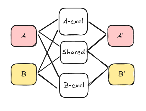
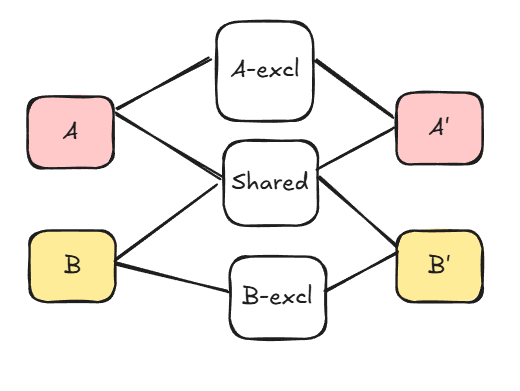
Figure 1: Three architectures for joint sparse decomposition of paired model activations. a — Crosscoders, b — Tied Crosscoders, c — Dedicated Feature Crosscoders
2.0.0.1 Sparse autoencoders and mechanistic interpretability.
SAEs are popular as a tool for decomposing LLM activations into interpretable features [2]–[4], [7]. These methods are built on the hypothesis that model representations are superpositions of many more features than there are neurons, and that sparse dictionary learning can recover them.
2.0.0.2 Crosscoders and model diffing.
Crosscoders [5] (fig. 1 (a)) extend SAEs to pairs of models by jointly encoding their activations into one shared sparse dictionary. Dedicated Feature Crosscoders [6] (fig. 1 (c)), like the Tied Crosscoders [8] (fig. 1 (b)), further partition this dictionary with gradient masking. It forces each model to read from and write to only its designated partition. Our work is the first systematic behavioral evaluation of DFC across a hyperparameter sweep, and the first to demonstrate single-neuron steering saturation.
2.0.0.3 RL fine-tuning for tool use.
ToolRL [9] demonstrates that RL from execution feedback substantially improves structured tool-call generation in
Qwen2.5-3B. We use the ToolRL-fine-tuned model as Model \(A\) throughout our experiments.
2.0.0.4 Activation steering.
Our steering approach operates in the sparse dictionary of the crosscoder which allows for feature-level intervention [4]. We identify the minimal steerable subset of neurons, and a single \(A\)-exclusive neuron is enough to maximize the effect.
2.0.0.5 Automated interpretability.
Automated interpretability methods [10] use LLM judges to label and score SAE features. We apply the protocol to validate \(A\)-exclusive feature interpretations.
3 Methodology↩︎
3.1 Models and Training Data↩︎
We study two models sharing the Qwen2.5-3B architecture (\(d=2048\), \(36\) layers): Model B (Base): Qwen/Qwen2.5-3B [11] and Model A (RL): chengq9/ToolRL-Qwen2.5-3B [9], RL-fine-tuned for structured <tool_call> invocation.
Training uses \(40{,}000\) FineWeb [12] samples (general-domain) and \(40{,}000\) ToolRL instruction-output pairs.
3.2 DFC Architecture and Training Objective↩︎
The DFC dictionary of size \(D\) is partitioned into A-exclusive \([0, a_\text{end})\), B-exclusive \([a_\text{end}, b_\text{end})\), and shared \([b_\text{end}, D)\) features, with gradient masking enforcing exclusivity. The training objective is presented in the Equation [1 ]: \[\begin{align} \mathcal{L} = {}& \mathrm{MSE}(h, \hat{h}) + \lambda_{\mathrm{sh}} \cdot \overline{\|f_{\mathrm{sh}}\|_1} \\ & + \frac{\lambda_{\mathrm{excl}}}{2}\left( \overline{\|f_{A\cup\mathrm{sh}}\|_1} + \overline{\|f_{B\cup\mathrm{sh}}\|_1} \right) \end{align} \label{eq:loss}\tag{1}\] where \(h=(h_A,h_B)\) is the concatenated residual stream post-MLP and \(\overline{|\cdot|_1}\) denotes the mean of \(|f_i|\). Top-\(k\) sparsity is enforced in the encoder.
3.3 Hyperparameter Sweep↩︎
The sweep varies five axes that determine the decomposition’s capacity, sparsity, and partition structure (Table 1). Architecture is the top-level choice between a standard Crosscoder (one unpartitioned dictionary jointly encoding both models) and a DFC (the same dictionary explicitly split into A-exclusive, B-exclusive, and shared sub-dictionaries via gradient masking). Dictionary size \(D\) is the total number of features the dictionary can represent. Top-\(k\) is the sparsity budget: at each forward pass, only the \(k\) highest-activating features are retained. Exclusive share \(p\) (DFC only) is the fraction of \(D\) allocated to each exclusive partition. \(\boldsymbol{\lambda_{\text{excl}}}\) is the magnitude penalty applied specifically to the exclusive partitions (in the CrossCoder rows of Table 1 we reuse the same coefficient on the equivalent unmasked features — see code release): setting it to \(0\) (“free”) lets exclusive features fire without extra cost, while \(10^{-3}\) (“penalised”) pushes the model to route signal through shared features unless exclusivity is needed which allows to test whether the exclusive partition behaves as a sink or a filter.
| Axis | Values |
|---|---|
| Architecture | CrossCoder (no exclusive partition), DFC |
| Dictionary \(D\) | 8,192 384 |
| Top-\(k\) | 45 |
| Exclusive share \(p\) (DFC) | 3% % % |
| \(\lambda_\text{excl}\) (DFC; reused for CC variants) | 0 (free) \(10^{-3}\) (penalised) |
3.4 Behavioral Scoring Rubric↩︎
Each generated response is scored on three metrics [9]:
format_accuracy:
<tool_call>present and JSON"name":"..."field present;tool_correctness: called name fuzzy-matches a numbered tool in the prompt;
overall_score \(\in\{-1,0,+1,+2\}\): \(+2\) = both correct, \(0\) = format only, \(+1\) = tool only, \(-1\) = neither. Evaluation: 100 held-out ToolRL prompts per sweep variant and 40 prompts per steering cell (seed 42), greedy decoding,
max_new_tokens=200,max_length=2048.
3.5 Neuron Identification and Targeted Steering↩︎
Features are ranked by Cohen’s \(d\) on tool-use vs.general-text activations [Eq. 2 ]: \[d_i = \frac{\mu^\text{tool}_i - \mu^\text{gen}_i}{\sqrt{(s^{\text{tool}\,2}_i + s^{\text{gen}\,2}_i)/2}} \label{eq:cohend}\tag{2}\] and filtered by firing rate (\(\rho^\text{tool}_i\geq0.3\), \(\rho^\text{gen}_i\leq0.1\)). Targeted steering applies an additive correction to Model A’s residual stream [Eq. 3 ]: \[h'_A = h_A + \sum_{i \in S} (\alpha-1)\cdot f_i \cdot W_\text{dec}[i,A,:] \label{eq:steer}\tag{3}\] for subset \(S\) of A-exclusive features ranked by \(d_i\), steering coefficient \(\alpha\), and decoder column \(W_\text{dec}[i,A,:]\in\mathbb{R}^d\). (Section 5).
4 Feature Space Analysis↩︎
4.1 DFC vs CrossCoder Decoder Geometry↩︎
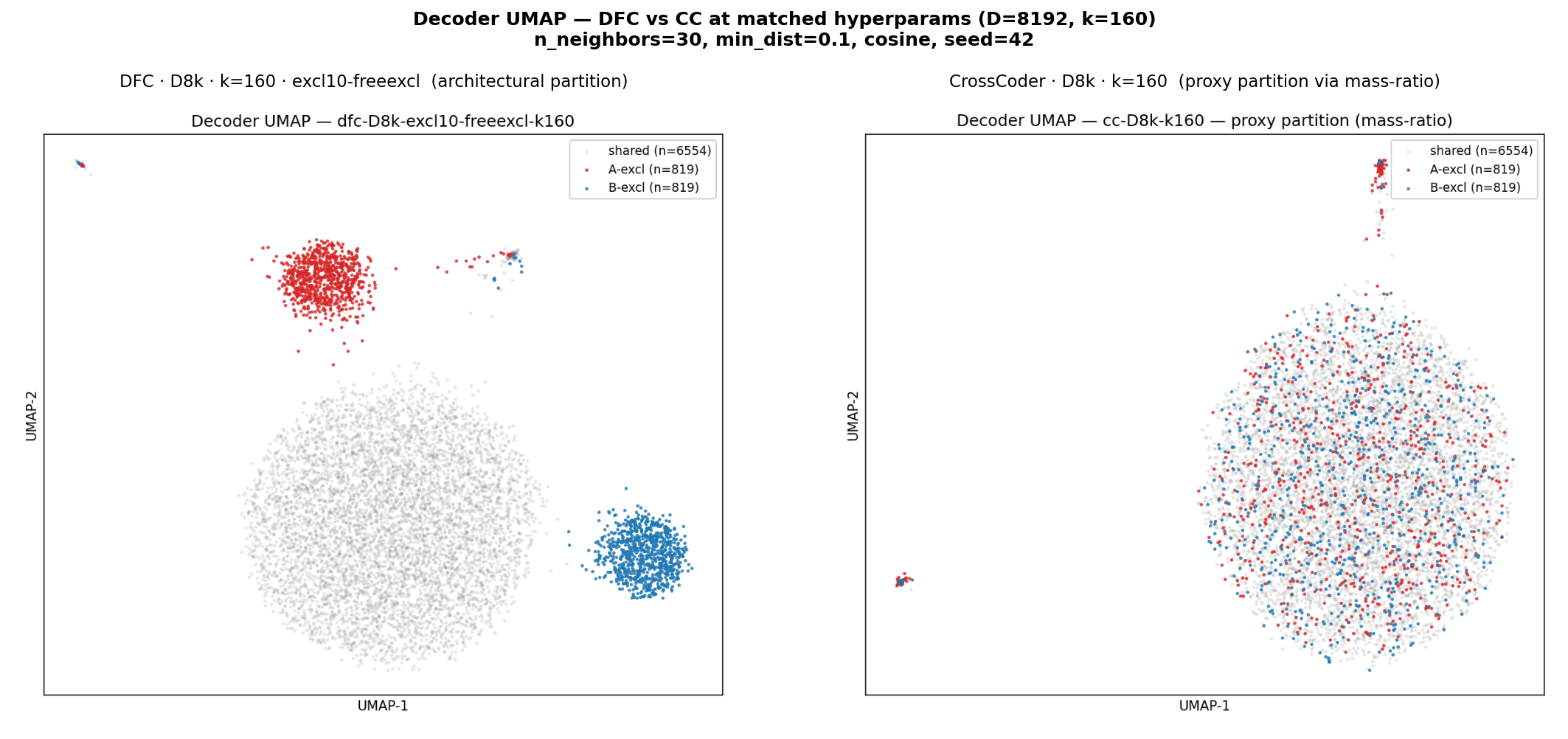
To test whether the partitioned geometry observed for the DFC (Figure 2) is a consequence of the gradient-mask architecture or merely of label imbalance, we construct a matched-size proxy partition for the unconstrained CrossCoder. For each dictionary feature \(i\), the decoder has two columns: \(W_{\text{dec}}[i, 0, :]\), the direction the feature decodes into Model A’s residual stream, and \(W_{\text{dec}}[i, 1, :]\), the direction it decodes into Model B’s. We define the mass-ratio \[r_i = \log\!\frac{\lVert W_{\text{dec}}[i, 0, :]\rVert_2}{\lVert W_{\text{dec}}[i, 1, :]\rVert_2}\] so that \(r_i \gg 0\) indicates a feature writing almost entirely into Model A (effectively A-exclusive), \(r_i \ll 0\) indicates Model B (effectively B-exclusive), and \(r_i \approx 0\) indicates balanced contribution (shared). For the DFC, the partition mask forces this ratio: the first \(819\) features have \(W_{\text{dec}}[i, 1, :] = 0\) (so \(r_i \to +\infty\)), the next \(819\) have \(W_{\text{dec}}[i, 0, :] = 0\) (\(r_i \to -\infty\)), and the remaining \(6{,}554\) have unconstrained A and B decoders. For the CrossCoder no such constraint exists, so we sort all \(8{,}192\) features by \(r_i\) and label the top \(819\) as the A-exclusive proxy, the bottom \(819\) as the B-exclusive proxy, and the middle \(6{,}554\) as the shared proxy. This produces partition slices of identical size to the DFC’s, so any difference in UMAP separation is attributable to the training objective (partition mask vs no mask) rather than to label imbalance.
With matched sizes, the CrossCoder’s A-biased features still mix uniformly with B-biased and shared features. The A-exclusive proxy in the CC has negative silhouette (\(-0.168\)) — on average, mass-ratio-A-biased features sit closer to non-A-biased centroids than to their own — and \(k\)-NN purity drops from the DFC’s \(0.984\) to \(0.158\), i.e.the precision of recovering A-exclusive proxy labels among an A-biased feature’s nearest neighbours falls to roughly the prior \(|A|/D \approx 10\%\), the chance level for a \(10\%\) minority class under random label assignment. HDBSCAN clusters in the CC UMAP recover the mass-ratio labels at ARI \(= 0.08\) versus \(0.93\) for the DFC: the structure simply isn’t there to be recovered. This falsifies the alternative explanation that the DFC’s clean separation is a UMAP artefact: with matched dictionary size (\(D = 8{,}192\)) and matched sparsity (\(k = 160\)), the same UMAP pipeline produces no separation when the partition mask is removed. The geometric structure in the DFC plot is caused by the architectural partitioning and mass-asymmetry alone is insufficient to produce it. The gradient mask reorganises feature directions, not just decoder magnitudes.
5 Reconstruction Fidelity and Capability Spillover↩︎
5.1 Sweep-Level Reconstruction↩︎
| Metric | Model A (ToolRL) | Model B (Base) |
|---|---|---|
| Pre-recon tool_correctness | 19% | 0% |
| Post-recon tool_correctness | 50.1% | \(6.8\)% |
| \(\Delta\) tool-correctness | \(+31.1\pm{9.7}\) pp | \(+6.8\pm5.0\) pp |
| \(\Delta\) overall_score | \(+0.93\) | \(+0.14\) |
| \(\Delta\) format_accuracy | substantial | \(+0\) pp identically |
Across the \(48\)-model sweep, reconstruction substantially improves the RL model’s behavioral performance relative to its pre-reconstruction baseline (Table 2). Every one of the \(48\) trained variants improves Model \(A\) tool correctness (\(48 / 48\)); under a one-sided exact-binomial sign test against the chance rate of \(0.5\), this corresponds to \(p \approx 3.6 \times 10^{-15}\).
At the same time, behavioral preservation (and even performance boost) does not track raw reconstruction loss in any simple way. Across the sweep, training MSE correlates only weakly with the gain in Model A performance (\(r=+0.08\), 95% CI \([-0.21,+0.36]\)). In other words, lower MSE does not reliably predict better behavioral reconstruction. This suggests that the information required for successful tool calling occupies a relatively sparse and behaviorally privileged subspace: a model can incur substantial activation-level distortion while still preserving the task-relevant structure needed to emit correct tool calls. One plausible interpretation is that the top-\(k\) bottleneck acts as an implicit regulariser, discarding noisy or behaviorally irrelevant components while retaining the sparse features most important for tool-use performance.
5.2 Capability Spillover↩︎
Model B’s tool-correctness rises from 0% to \(6.8\%\) post-reconstruction (paired-\(t\) across the \(48\) runs against the always-zero baseline: \(t \approx 9.4\), \(p \approx 1\times10^{-12}\)) without any fine-tuning. We call this capability spillover: tool-calling intent is delocalized into the shared decoder weights during joint training and reconstruction passively routes it into Model B’s activation stream.
Format accuracy never spills over (\(\Delta_B\) format \(=0\) pp across all 48 runs). Model B correctly identifies tools in prose but never produces the exact
<tool_call>..."name":... surface form. It suggests that semantic tool-selection intent is at least partially represented in shared directions, but the exact surface-form machinery required to produce the <tool_call>
template remains isolated in narrow RL-specific features. This interpretation is consistent with the later autointerp evidence, which shows that the most discriminative A-exclusive features are structural-template detectors rather than broad abstract
tool-use concepts.
5.3 Architecture Comparison↩︎
| Arch. | \(n\) | \(\Delta A\) (pp) | \(\Delta B\) (pp) | Train MSE |
|---|---|---|---|---|
| CrossCoder | 12 | \(+32.9\) | \(+8.9\) | \(0.031\pm0.010\) |
| DFC | 36 | \(+30.5\) | \(+6.1\) | \(0.031\pm0.007\) |
Comparing the two architectures at sweep level (Table 3), CrossCoders and DFCs achieve essentially indistinguishable reconstruction error but somewhat different behavioral transfer profiles. CrossCoders (\(12\) runs) achieve a mean Model A tool-correctness gain of \(+32.9\) pp and a mean Model B gain of \(+8.9\) pp, while DFCs (36 runs) achieve \(+30.5\) pp on Model A and \(+6.1\) pp on Model B. Mean training MSE is the same to three decimal places for both families. Raw reconstruction loss alone does not explain the behavioral differences.
The directional reduction in Model B spillover under DFC is suggestive but not statistically decisive in this sweep. A Welch’s \(t\)-test on \(\Delta_B\) yields \(t=1.63\), \(p=0.12\), so we do not claim a significant architecture-level difference here. The more cautious interpretation is that DFC may reduce spillover relative to an unpartitioned CrossCoder, but the evidence is currently underpowered and should be treated as directional rather than conclusive.
5.4 The DFC Partition as a Filter, Not a Sink↩︎
\(\lambda_{\text{excl}} = 10^{-3}\) reduces Model \(A\) fidelity relative to \(\lambda_{\text{excl}} = 0\) at both the \(5\%\) and \(10\%\) exclusive shares (\(34.8 \to 25.8\) pp \(\Delta A\) at \(5\%\) and \(35.2 \to 32.0\) pp at \(10\%\), each averaged over the six matched \((D,k)\) pairs in Appendix 10, Table 1). Sparsifying the exclusive partition therefore pushes tool-specific signal back into the shared partition rather than removing it. Rather than isolating all RL-specific signal into a protected compartment, the exclusive partition appears to act more like a filter that concentrates the most model-specific residue.
If the exclusive slice were a true sink for the capability difference, sparsifying it should mostly remove redundant or nonessential signal while leaving shared structure intact. Instead, penalizing the exclusive slice appears to push some tool-relevant information back into the shared partition, where it is both less behaviorally efficient for Model \(A\) and more available for spillover into Model \(B\). The DFC partition therefore helps localize model-specific features, but it does not perfectly disentangle capability-specific content from the shared representational substrate.
6 Targeted-Neuron Steering↩︎
6.1 DFC Saturates at a Single Feature↩︎
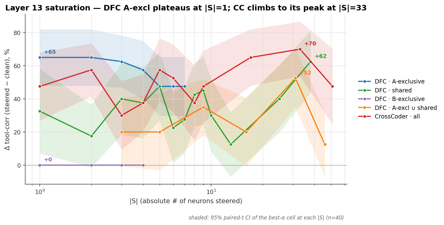
Steering a single A-exclusive neuron (\(|S|=1\), \(\alpha=32\)) achieves \(\mathbf{+65.0}\) pp \(\Delta\) tool-correctness (95% CI \([+47.9,+82.1]\)), matching the performance of steering all 7 available A-exclusive neurons. CrossCoder requires \(|S|=33\) to reach its unbudgeted peak of \(+70.0\) pp (\([+53.5,+86.5]\)) (Fig. 3). DFC A-exclusive plateaus immediately; CC climbs slowly across \(33\times\) the budget. The full per-\(|S|\) breakdown with CIs is in Table 9 (Appendix 11).
6.2 Ablation Studies↩︎
Table 4 isolates four mechanisms. B-exclusive steering has zero effect at every cell. A-exclusive beats shared under a small budget, despite shared holding more tool-relevant features by Cohen’s \(d\). Signal in A-exclusive is concentrated; signal in shared is diffuse. Steering A-exclusive and shared together underperforms A-exclusive alone. The likely cause is destructive interference between non-orthogonal decoder directions amplified at matched \(\alpha\). The unpartitioned CrossCoder eventually matches DFC A-exclusive’s peak, but only by recruiting an order of magnitude more features.
| Condition | Best \(\Delta\) (%) | 95% CI | \(|S|\) | \(\alpha\) |
|---|---|---|---|---|
| Within \(|S|\leq10\) | ||||
| DFC \(\cdot\) A-exclusive | +65.0 | [+47.9,+82.1] | 1 | 32 |
| DFC \(\cdot\) shared | +47.5 | [+27.0,+68.0] | 5 | 16 |
| DFC \(\cdot\) B-exclusive | +0.0 | [+0.0,+0.0] | 1 | 1 |
| DFC \(\cdot\) A-excl \(\cup\) shared | +35.0 | [+17.9,+52.1] | 9 | 16 |
| CrossCoder \(\cdot\) all | +57.5 | [+41.5,+73.5] | 2 | 32 |
| Unbudgeted (any \(|S|\)) | ||||
| DFC \(\cdot\) A-exclusive | +65.0 | [+47.9,+82.1] | 1 | 32 |
| DFC \(\cdot\) shared | +62.5 | [+43.8,+81.2] | 38 | 6 |
| CrossCoder \(\cdot\) all | +70.0 | [+53.5,+86.5] | 33 | 6 |
6.3 DFC vs CrossCoder: Budget-Dependent Advantage↩︎
DFC A-exclusive significantly outperforms shared, B-exclusive, and the A-excl \(\cup\) shared combination, with effect sizes ranging from moderate (\(d_z = 0.40\)) to very large (\(d_z = 1.03\)) (Table 5). Against the unconstrained CrossCoder, the difference is null (\(d_z = 0.00\), \(p = 0.51\)). Within the power of this study, the two architectures’ unbudgeted ceilings are indistinguishable. This is the central tradeoff. The DFC’s value is that it reaches its ceiling with one neuron, whereas the CrossCoder needs thirty-three to reach its. For interpretability and targeted intervention, single-neuron control is qualitatively different from distributed control; for raw behavioral effect at any cost, the architectures are interchangeable.
| Comparison | Mean \(\Delta\) (pp) | Cohen’s \(d_z\) | \(p\) (one-sided) |
|---|---|---|---|
| A-excl \(-\) shared | +10.5 | 0.40 | 0.019 |
| A-excl \(-\) B-excl | +24.3 | 1.03 | \(2.2\times10^{-6}\) |
| A-excl \(-\) combo | +15.7 | 0.56 | 0.002 |
| A-excl \(-\) CC | \(-\)0.08 | 0.00 | 0.51 (n.s.) |
6.4 Cross-Layer Generalisation↩︎
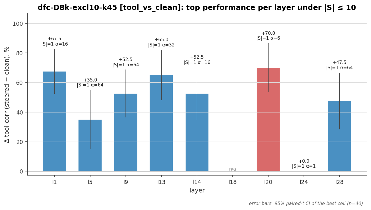
Across-layers (fig. 4), the mean best-cell is \(\Delta=+43.3\) pp (95% CI \([+22.7,+64.0]\)), Cohen’s \(d_z=1.61\), and paired \(t\) \(p=0.0006\), Wilcoxon \(p=0.0078\). Single-neuron saturation is not a layer-\(13\) artefact.
6.5 B-Exclusive Steering Has No Effect↩︎
B-exclusive steering produces \(\Delta=+0.0\) pp at every \((|S|,\alpha)\) cell (CI \([+0.0,+0.0]\)). We include this comparison as an end-to-end sanity check on the steering harness rather than a behavioural baseline: by construction, B-exclusive decoder columns have their Model-A output zeroed by the gradient mask, so any non-zero effect here would indicate a bug in our patching pipeline (wrong layer, wrong projection, leaked gradient). The flat \(+0.0\) pp result therefore confirms that the harness is working as intended, and the magnitude of the A-excl effect (\(d_z=1.03\), \(p=2.2\times10^{-6}\), Table 5) is being read out faithfully.
6.6 Combining A-excl and Shared Causes Interference↩︎
Steering A-excl \(\cup\) shared simultaneously is worse than either alone: the best combo \(+35.0\) pp at \(|S|=9\) vs A-excl \(+65.0\) pp at \(|S|=1\) (prompt-paired one-sided \(t\) across the \(n=40\) ToolRL prompts shared by both cells, \(p=0.002\), Cohen’s \(d_z=0.56\); the \(30\) shared \((|S|,\alpha)\) cells in Table 5 aggregate these prompt-level paired tests across cells). The most likely mechanism is destructive interference between non-orthogonal A-excl and shared decoder directions boosted at equal \(\alpha\).
6.7 Autointerp of the most important neuron↩︎
\(A\)-exclusive features (such as feat. \(\#136\) from figure 5) are structural-template detectors. They fire on narrow formatting
markers (<tool_call>, <response>, parameter boilerplate). The max-activating fragment receives the explanation (pseudocode from Appendix 8): “the structure of a dialogue
system, specifically the interaction between a tool call and a subsequent response.” DFC partitioning concentrates this detector in A-exclusive parameter space. Cohen’s \(d\) values larger than \(\sim 5\) here reflect a near-zero variance under the general-text condition (the feature simply does not fire there) and should be read as “cleanly separated” rather than as comparable effect sizes; the AUROC numbers, as used
in Appendix 9 for another device, are the more meaningful ranking signal.
6.8 Hypotheses Summary↩︎
Please see Table 6.
| H | Claim | Status | Key evidence | Section |
|---|---|---|---|---|
| H1 | Steering helps overall | confirmed | Cross-layer; paired-\(t\) \(p=0.0006\), Wilcoxon \(p=0.0078\) | §[sec:sec:crosslayer] |
| H2 | A-excl \(\gg\) B-excl | confirmed | \(d_z=1.03\), \(p=2.2\times10^{-6}\) | §[sec:sec:bexcl] |
| H3 | A-excl \(>\) shared at small \(|S|\) | confirmed | Pooled \(d_z{=}0.40\), \(p{=}0.019\) | §[sec:sec:budget] |
| H4 | DFC \(\not>\) CC unbudgeted | confirmed | \(p=0.51\) | §[sec:sec:budget] |
| H5 | DFC \(>\) CC at small \(|S|\) | confirmed | \(|S|=1\) gap \(+17.5\) pp | §[sec:sec:budget] |
| H6 | DFC saturates faster | confirmed | A-excl plateaus \(|S|=1\); CC needs 33 | §[sec:sec:saturation] |
| H7 | Combo \(>\) either alone | rejected | Best combo \(+35\) vs A-excl \(+65\) | §[sec:sec:interference] |
| H8 | Layer-13 generalises | confirmed | 7/9 layers \(\geq+35\) pp at \(|S|=1\) | §[sec:sec:crosslayer] |
7 Discussion↩︎
7.0.0.1 Joint training delocalises capability.
Our results partially refute the DFC’s design intent: that the exclusive partition cleanly contains the model-specific capability. Tool-calling capability survives in the shared decoder weights well enough to result in \(+6.8\) pp spillover to Model B and to make \(\lambda_\text{excl}\) penalisation hurt Model A fidelity. This is empirical evidence that superposition crosses model boundaries in joint sparse decompositions when underlying capabilities are not orthogonal in residual-stream space.
7.0.0.2 A minimal feature set carries most of the signal.
UMAP+HDBSCAN finds tens of clustered features out of 819 A-exclusive; the discrimination ranking concentrates Cohen’s \(d\) in single-digit feature indices; and a single feature suffices for maximum steering effect across 7 of 9 probed layers. This suggests that sparse-feature-level interpretability of agentic capabilities works.
7.0.0.3 Capability transfer is a side channel.
The fact that a frozen base model gains \(+6.8\) pp tool-correctness purely from the decomposition pipeline, with no fine-tuning, suggests that releasing crosscoders trained between model pairs with different capability levels may inadvertently provide a substrate that reintroduces the capability at inference time.
7.0.0.4 Steering as low-intervention behavioral control.
We find that \(+65\) pp tool-correctness from a post-top-\(k\) delta on a single feature requires zero retraining. The same machinery can in principle suppress unwanted behaviors by clamping the corresponding features to zero, positioning DFC-based steering alongside RLHF/DPO/SFT for safety post-training with the advantages of being inference-time, gradient-free, and inspectable.
7.0.0.5 Limitations.
We use “capability” as shorthand for reliable, structured tool-call generation. We do not claim RL installs a tool-use ability the base model wholly lacks. Our metrics measure the propensity to emit correct tool calls under a fixed evaluation prompt, and we did not run a prompted baseline tuned to maximally elicit base-model tool use; our interventions should be read as modulating this propensity. We study a single model pair (Qwen2.5-3B) and a single task (ToolRL). The architecture-effect \(t\)-test is underpowered (12 CC vs 36 DFC runs). The steering results come from \(n=40\) prompts per cell; the best-cell numbers have not been replicated on a fresh sample. The autointerp pass covered only A-exclusive features (Section 6.7); the shared partition is the natural next target given that it carries most of the spilled tool capability.
7.0.0.6 Future Work.
Since RL shapes agents that take consequential actions, the behaviors RL installs should become objects we can monitor and steer. Model diffing is a step toward that because if RL-induced behaviors reliably condense into small feature sets, then steering them offers runtime control that complements RLHF, DPO, and SFT, with the advantage of being legible. Realising this vision will depend on having robust diffing methods; Delta-Crosscoders [13], which explicitly model the asymmetric nature of fine-tuning, are a promising path toward the fidelity such control would require. A further frontier is knowledge-boundary discovery [14]: the most consequential thing an agent decides is often whether to act at all. Locating the features that govern the boundary between committing to an action and abstaining under uncertainty would let us inspect an agent’s willingness to act.
Acknowledgments↩︎
We appreciate Prof. Manling Li’s guidance on the task selection and future work directions. We are thankful to Thomas Jiralerspong for clarifying our questions about the architecture and setup. We are grateful to Yuliia Tkachuk for her help with the visualizations (Fig. 1). This work was supported in part by the Northwestern University Department of Computer Science. We also thank Prof. Hullman for additional support.
8 Autointerp Pseudocode↩︎
AUTOINTERP(features, texts, K=10):
  # Stage 1: Find top-K activating examples per feature
  for each shard in feature_cache:
    for each feature f:
      maintain min-heap of size K by activation value

  # Stage 2: Explain
  for each feature f where topk[f] is non-empty:
    top_texts = lookup texts for topk[f]
    explanation = LLM("what pattern do these texts share?", top_texts)

  # Stage 3: Score (detection task)
    positives = top_texts              # should match explanation
    negatives = sample K random texts  # should not match
    combined  = shuffle(positives + negatives)
    predictions = LLM("MATCH or NO_MATCH?", explanation, combined)
    score = accuracy(predictions, ground_truth)
    interpretable = score >= 0.8
9 Top A-Exclusive Feature Interpretations↩︎
From dfc-D8k-excl10-freeexcl-k160, \(n=40\) prompts, ToolRL test split.
| Feat | Cohen’s \(d\) | AUROC | Det. | Gemma explanation |
|---|---|---|---|---|
| 521 | 12.18 | 0.998 | 0.80 | LM instructed to use tools for user requests |
| 730 | 4.80 | 0.954 | 0.50 | Retrieving info via unique identifiers |
| 538 | 4.43 | 0.949 | 0.80 | Instructions/guidelines for tool calls |
| 126 | 4.12 | 0.929 | 0.75 | Referencing previous conversation turns |
| 636 | 2.36 | 0.826 | 0.55 | LM interacting with tools and external APIs |
| 17 | 2.12 | 0.901 | 0.50 | Structured data input in dialogue systems |
| 583 | 1.92 | 0.882 | 0.70 | Structure and syntax of <tool_call> |
| 786 | 1.66 | 0.892 | 0.70 | Requests requiring external tools |
| 10 | 0.90 | 0.635 | 0.90 | Dialogue-system tool interactions, past refs |
| 708 | 0.84 | 0.588 | 0.80 | Using a tool with specific parameters |
10 Full Sweep Evaluation Table↩︎
Table 1 reports the key hyperparameters and post-reconstruction evaluation outcomes for all \(48\) evaluated sweep variants. We include both Model A and Model B post-reconstruction metrics so that individual model configurations can be cited directly in the appendix without referring back to the JSONL artifact.
| Model | Arch | \(D\) | \(k\) | \(p\) | \(\lambda_{\mathrm{excl}}\) | \(\lambda_{\mathrm{sh}}\) | A ov | A fmt | A tool | \(\Delta\)A tool | B ov | B fmt | B tool | \(\Delta\)B tool | |
|---|---|---|---|---|---|---|---|---|---|---|---|---|---|---|---|
| Table (continued) | |||||||||||||||
| Model | Arch | \(D\) | \(k\) | \(p\) | \(\lambda_{\mathrm{excl}}\) | \(\lambda_{\mathrm{sh}}\) | A ov | A fmt | A tool | \(\Delta\)A tool | B ov | B fmt | B tool | \(\Delta\)B tool | |
| Continued on next page | |||||||||||||||
cc-D16k-k160 |
CrossCoder | 16384 | 160 | 0% | 0 | \(10^{-3}\) | 1 | 66 | 67 | 48 | -0.92 | 0 | 4 | 4 | |
cc-D16k-k45 |
CrossCoder | 16384 | 45 | 0% | 0 | \(10^{-3}\) | 0.55 | 51 | 52 | 33 | -0.76 | 0 | 12 | 12 | |
cc-D16k-k90 |
CrossCoder | 16384 | 90 | 0% | 0 | \(10^{-3}\) | 0.37 | 45 | 46 | 27 | -0.94 | 0 | 3 | 3 | |
cc-D16k-nol1-k160 |
CrossCoder | 16384 | 160 | 0% | 0 | 0 | 0.26 | 42 | 42 | 23 | -0.70 | 0 | 15 | 15 | |
cc-D16k-nol1-k45 |
CrossCoder | 16384 | 45 | 0% | 0 | 0 | 0.59 | 53 | 53 | 34 | -0.72 | 0 | 14 | 14 | |
cc-D16k-nol1-k90 |
CrossCoder | 16384 | 90 | 0% | 0 | 0 | 0.05 | 35 | 35 | 16 | -0.70 | 0 | 15 | 15 | |
cc-D8k-k160 |
CrossCoder | 8192 | 160 | 0% | 0 | \(10^{-3}\) | 0.47 | 49 | 49 | 30 | -0.92 | 0 | 4 | 4 | |
cc-D8k-k45 |
CrossCoder | 8192 | 45 | 0% | 0 | \(10^{-3}\) | 0.76 | 58 | 59 | 40 | -0.76 | 0 | 12 | 12 | |
cc-D8k-k90 |
CrossCoder | 8192 | 90 | 0% | 0 | \(10^{-3}\) | 0.50 | 50 | 50 | 31 | -0.94 | 0 | 3 | 3 | |
cc-D8k-nol1-k160 |
CrossCoder | 8192 | 160 | 0% | 0 | 0 | 0.21 | 41 | 40 | 21 | -0.84 | 0 | 8 | 8 | |
cc-D8k-nol1-k45 |
CrossCoder | 8192 | 45 | 0% | 0 | 0 | 1.10 | 70 | 70 | 51 | -0.66 | 0 | 17 | 17 | |
cc-D8k-nol1-k90 |
CrossCoder | 8192 | 90 | 0% | 0 | 0 | 0.80 | 60 | 60 | 41 | -1 | 0 | 0 | 0 | |
dfc-D16k-excl10-freeexcl-k160 |
DFC | 16384 | 160 | 10% | 0 | \(10^{-3}\) | 0.75 | 59 | 58 | 39 | -0.92 | 0 | 4 | 4 | |
dfc-D16k-excl10-freeexcl-k45 |
DFC | 16384 | 45 | 10% | 0 | \(10^{-3}\) | -0.01 | 33 | 33 | 14 | -0.98 | 0 | 1 | 1 | |
dfc-D16k-excl10-freeexcl-k90 |
DFC | 16384 | 90 | 10% | 0 | \(10^{-3}\) | 0.69 | 57 | 56 | 37 | -0.62 | 0 | 19 | 19 | |
dfc-D16k-excl10-k160 |
DFC | 16384 | 160 | 10% | \(10^{-3}\) | \(10^{-3}\) | 0.60 | 52 | 54 | 35 | -0.90 | 0 | 5 | 5 | |
dfc-D16k-excl10-k45 |
DFC | 16384 | 45 | 10% | \(10^{-3}\) | \(10^{-3}\) | 0.54 | 50 | 52 | 33 | -0.86 | 0 | 7 | 7 | |
dfc-D16k-excl10-k90 |
DFC | 16384 | 90 | 10% | \(10^{-3}\) | \(10^{-3}\) | 0.54 | 50 | 52 | 27 | -0.70 | 0 | 15 | 15 | |
dfc-D16k-excl3-freeexcl-k160 |
DFC | 16384 | 160 | 3% | 0 | \(10^{-3}\) | 0.49 | 49 | 50 | 31 | -0.94 | 0 | 3 | 3 | |
dfc-D16k-excl3-freeexcl-k45 |
DFC | 16384 | 45 | 3% | 0 | \(10^{-3}\) | 0.49 | 49 | 50 | 31 | -0.88 | 0 | 6 | 6 | |
dfc-D16k-excl3-freeexcl-k90 |
DFC | 16384 | 90 | 3% | 0 | \(10^{-3}\) | 0.23 | 41 | 41 | 22 | -0.82 | 0 | 9 | 9 | |
dfc-D16k-excl3-k160 |
DFC | 16384 | 160 | 3% | \(10^{-3}\) | \(10^{-3}\) | 0.56 | 52 | 52 | 33 | -0.84 | 0 | 8 | 8 | |
dfc-D16k-excl3-k45 |
DFC | 16384 | 45 | 3% | \(10^{-3}\) | \(10^{-3}\) | 0.28 | 42 | 43 | 24 | -0.88 | 0 | 6 | 6 | |
dfc-D16k-excl3-k90 |
DFC | 16384 | 90 | 3% | \(10^{-3}\) | \(10^{-3}\) | 0.26 | 42 | 42 | 23 | -0.86 | 0 | 7 | 7 | |
dfc-D16k-excl5-freeexcl-k160 |
DFC | 16384 | 160 | 5% | 0 | \(10^{-3}\) | 0.74 | 58 | 58 | 39 | -0.94 | 0 | 3 | 3 | |
dfc-D16k-excl5-freeexcl-k45 |
DFC | 16384 | 45 | 5% | 0 | \(10^{-3}\) | 0.44 | 48 | 48 | 29 | -0.88 | 0 | 6 | 6 | |
dfc-D16k-excl5-freeexcl-k90 |
DFC | 16384 | 90 | 5% | 0 | \(10^{-3}\) | 0.33 | 43 | 45 | 26 | -0.86 | 0 | 7 | 7 | |
dfc-D16k-excl5-k160 |
DFC | 16384 | 160 | 5% | \(10^{-3}\) | \(10^{-3}\) | 0.49 | 49 | 50 | 31 | -0.92 | 0 | 4 | 4 | |
dfc-D16k-excl5-k45 |
DFC | 16384 | 45 | 5% | \(10^{-3}\) | \(10^{-3}\) | 0.37 | 45 | 46 | 27 | -0.94 | 0 | 3 | 3 | |
dfc-D16k-excl5-k90 |
DFC | 16384 | 90 | 5% | \(10^{-3}\) | \(10^{-3}\) | 0.49 | 49 | 50 | 31 | -0.94 | 0 | 3 | 3 | |
dfc-D8k-excl10-freeexcl-k160 |
DFC | 8192 | 160 | 10% | 0 | \(10^{-3}\) | 1.49 | 83 | 83 | 64 | -1 | 0 | 0 | 0 | |
dfc-D8k-excl10-freeexcl-k45 |
DFC | 8192 | 45 | 10% | 0 | \(10^{-3}\) | 0.27 | 41 | 43 | 24 | -0.88 | 0 | 6 | 6 | |
dfc-D8k-excl10-freeexcl-k90 |
DFC | 8192 | 90 | 10% | 0 | \(10^{-3}\) | 0.56 | 52 | 52 | 33 | -0.82 | 0 | 9 | 9 | |
dfc-D8k-excl10-k160 |
DFC | 8192 | 160 | 10% | \(10^{-3}\) | \(10^{-3}\) | 0.32 | 44 | 44 | 25 | -0.84 | 0 | 8 | 8 | |
dfc-D8k-excl10-k45 |
DFC | 8192 | 45 | 10% | \(10^{-3}\) | \(10^{-3}\) | 0.70 | 56 | 57 | 38 | -0.60 | 0 | 20 | 20 | |
dfc-D8k-excl10-k90 |
DFC | 8192 | 90 | 10% | \(10^{-3}\) | \(10^{-3}\) | 0.60 | 54 | 53 | 34 | -0.96 | 0 | 2 | 2 | |
dfc-D8k-excl3-freeexcl-k160 |
DFC | 8192 | 160 | 3% | 0 | \(10^{-3}\) | 0.68 | 56 | 56 | 37 | -0.88 | 0 | 6 | 6 | |
dfc-D8k-excl3-freeexcl-k45 |
DFC | 8192 | 45 | 3% | 0 | \(10^{-3}\) | 0.47 | 49 | 49 | 30 | -0.88 | 0 | 6 | 6 | |
dfc-D8k-excl3-freeexcl-k90 |
DFC | 8192 | 90 | 3% | 0 | \(10^{-3}\) | 0.10 | 36 | 37 | 18 | -0.82 | 0 | 9 | 9 | |
dfc-D8k-excl3-k160 |
DFC | 8192 | 160 | 3% | \(10^{-3}\) | \(10^{-3}\) | 0.50 | 50 | 50 | 31 | -0.90 | 0 | 5 | 5 | |
dfc-D8k-excl3-k45 |
DFC | 8192 | 45 | 3% | \(10^{-3}\) | \(10^{-3}\) | 0.32 | 44 | 44 | 25 | -0.98 | 0 | 1 | 1 | |
dfc-D8k-excl3-k90 |
DFC | 8192 | 90 | 3% | \(10^{-3}\) | \(10^{-3}\) | 0.32 | 44 | 44 | 25 | -0.88 | 0 | 6 | 6 | |
dfc-D8k-excl5-freeexcl-k160 |
DFC | 8192 | 160 | 5% | 0 | \(10^{-3}\) | 0.53 | 51 | 51 | 32 | -0.92 | 0 | 4 | 4 | |
dfc-D8k-excl5-freeexcl-k45 |
DFC | 8192 | 45 | 5% | 0 | \(10^{-3}\) | 0.71 | 57 | 57 | 38 | -0.96 | 0 | 2 | 2 | |
dfc-D8k-excl5-freeexcl-k90 |
DFC | 8192 | 90 | 5% | 0 | \(10^{-3}\) | 0.92 | 64 | 64 | 45 | -0.94 | 0 | 3 | 3 | |
dfc-D8k-excl5-k160 |
DFC | 8192 | 160 | 5% | \(10^{-3}\) | \(10^{-3}\) | -0.22 | 26 | 26 | 7 | -0.96 | 0 | 2 | 2 | |
dfc-D8k-excl5-k45 |
DFC | 8192 | 45 | 5% | \(10^{-3}\) | \(10^{-3}\) | 0.35 | 45 | 45 | 26 | -0.94 | 0 | 3 | 3 | |
dfc-D8k-excl5-k90 |
DFC | 8192 | 90 | 5% | \(10^{-3}\) | \(10^{-3}\) | 0.55 | 51 | 52 | 33 | -0.74 | 0 | 13 | 13 | |
11 Full Saturation Table↩︎
Best \(\Delta\) tool-correctness (max over \(\alpha\)) at each \(|S|\) with 95% paired-\(t\) CIs, referenced from Section 6.1. “—” indicates no sweep coverage.
| \(|S|\) | DFC A-excl | DFC shared | CC | A-excl \(-\) CC |
|---|---|---|---|---|
| 1 | +65.0 [+47.9, +82.1] | +32.5 [+7.0, +58.0] | +47.5 [+27.0, +68.0] | +17.5 |
| 2 | +65.0 [+47.9, +82.1] | +17.5 [\(-\)1.5, +36.5] | +57.5 [+41.5, +73.5] | +7.5 |
| 3 | +62.5 [+46.8, +78.2] | +40.0 [+18.5, +61.5] | +30.0 [+9.3, +50.7] | +32.5 |
| 4 | +57.5 [+39.9, +75.1] | +37.5 [+16.2, +58.8] | +37.5 [+20.2, +54.8] | +20.0 |
| 5 | +47.5 [+29.8, +65.2] | +47.5 [+27.0, +68.0] | +57.5 [+38.5, +76.5] | \(-\)10.0 |
| 6 | +47.5 [+29.8, +65.2] | +22.5 [+1.4, +43.6] | +52.5 [+32.0, +73.0] | \(-\)5.0 |
| 7 | +47.5 [+29.8, +65.2] | +27.5 [+7.0, +48.0] | — | — |
| 8 | — | +42.5 [+23.5, +61.5] | +37.5 [+15.0, +60.0] | — |
| 9 | — | +45.0 [+24.6, +65.4] | +47.5 [+25.8, +69.2] | — |
| 10 | — | +30.0 [+8.0, +52.0] | — | — |
| 33 | — | — | +70.0 [+53.5, +86.5] | — |
| 38 | — | +62.5 [+43.8, +81.2] | — | — |

11.1 Practical Sweet Spot and \(\alpha\) Tradeoff↩︎
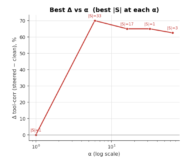
Key operating points: DFC A-excl at \(|S|=1\), \(\alpha=32\) yields \(+65.0\) pp; CC at \(|S|=33\), \(\alpha=6\) yields \(+70.0\) pp — \(33\times\) the neuron budget for a \(5\) pp gain. Over-steering (\(\alpha=64\), \(|S|\geq9\)) degrades performance (e.g. \(|S|=33\), \(\alpha=64\to+0.0\) pp).
11.2 Per-Condition Heatmaps↩︎

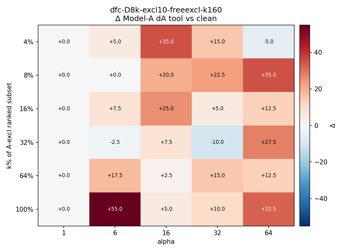
Figure 7: Per-cell \(\Delta\) tool-correctness heatmaps (\(|S|\times\alpha\)) for the two representative DFCs. Sparse \(k=45\) peaks at
targeted low-\(|S|\) steering; dense \(k=160\) benefits from broader coverage.. a — dfc-D8k-excl10-k45: sweet spot at low \(|S|\), high \(\alpha\)., b — dfc-D8k-excl10-freeexcl-k160: sweet spot at high \(|S|\), moderate \(\alpha\).
12 Models and Repository↩︎
Our code can be found at https://github.com/Antebe/model_diffing_crosscoders. The full sweep is now available at https://huggingface.co/collections/antebe1/qwen-toolrl-crosscoder.
References↩︎
see Limitations (section sec:sec:sec:discussion?)↩︎
A sink is the limiting case of a filter. It is reached only when the capability is orthogonal to shared structure.↩︎